Embed Size (px)
Citation preview
Purdue UniversityPurdue e-Pubs
Open Access Dissertations Theses and Dissertations
Fall 2014
Model-based powertrain design and control systemdevelopment for the ideal all-wheel drive electricvehicleHaotian WuPurdue University
Follow this and additional works at: https://docs.lib.purdue.edu/open_access_dissertations
Part of the Mechanical Engineering Commons
This document has been made available through Purdue e-Pubs, a service of the Purdue University Libraries. Please contact [email protected] foradditional information.
Recommended CitationWu, Haotian, "Model-based powertrain design and control system development for the ideal all-wheel drive electric vehicle" (2014).Open Access Dissertations. 392.https://docs.lib.purdue.edu/open_access_dissertations/392
30 08 14
PURDUE UNIVERSITY GRADUATE SCHOOL
Thesis/Dissertation Acceptance
Department
To the best of my knowledge and as understood by the student in the Thesis/Dissertation Agreement, Publication Delay, and Certification/Disclaimer (Graduate School Form 32), this thesis/dissertationadheres to the provisions of Purdue University’s “Policy on Integrity in Research” and the use of copyrighted material.
Haotian Wu
MODEL-BASED POWERTRAIN DESIGN AND CONTROL SYSTEM DEVELOPMENTFOR THE IDEAL ALL-WHEEL DRIVE ELECTRIC VEHICLE
Doctor of Philosophy
Haiyan H. Zhang Richard M. French
Qingyou Han Ayhan Ince
Haiyan H. Zhang
James L. Mohler 11/14/2014

MODEL-BASED POWERTRAIN DESIGN AND CONTROL SYSTEM DEVELOPMENT
FOR THE IDEAL ALL-WHEEL DRIVE ELECTRIC VEHICLE
A Dissertation
Submitted to the Faculty
of
Purdue University
by
Haotian Wu
In Partial Fulfillment of the
Requirements for the Degree
of
Doctor of Philosophy
December 2014
Purdue University
West Lafayette, Indiana
ii
ACKNOWLEDGEMENTS
I would like to express my deep gratitude to my advisor Haiyan H. Zhang. It has
been an honor to be one of his Ph.D. students. I massively appreciate all his
contributions of efforts, funding and ideas to make my Ph.D. experience joyful. He is my
primary resource to get my research questions answered and obtain strong support
during tough times in the Ph.D. pursuit. Haiyan is one of the most diligent and smartest
people I know. I have been grateful for all the help from the members in his lab,
Multidisciplinary Lab. I also deliver my sincere thanks to Siemens PLM Software that
donated LMS Imagine.Lab Amesim for my research.
In addition, I really want to thank the professors in my academic committee,
Professors Qingyong Han, Richard M. French and Ayhan Ince for their helpful career
advice and many insightful research discussions. I have also appreciated the professors
in Purdue EcoCar2 Project, Professors Haiyan H. Zhang, Peter Meckl, Gregory M. Shaver,
Oleg Wasynczuk, and Motevalli Vahid for helping me to cast my leadership and
instructing me to see the research at different angles. Moreover, I massively appreciate
that Prof. James L. Mohler provided valuable suggestions about the dissertation
formatting and editing.
I will forever be thankful to my former research advisor, Professor Xuexun Guo.

iii
He has been helpful in providing invaluable advice to pursue my Ph.D. degree at Purdue
University. I still think fondly of my time as an undergraduate student and M.S. student
in his lab. I also am very grateful to Yuanhai Ou, Professors Guofang Zhang and Yaohua
He for their continuous support during my college and graduate school career.
I also thank my friends for providing moral support and encouragement to the
research. I would like to thank Cong Liao, Xiao Yuan and Xinyue Chang for their support
in general. I am also thankful to Jiameng Wang for her tremendous help. It is too many
friends to be listed here, but I believe you can feel my deep gratitude.
I especially express my thanks from the underside of my affection to my mom,
papa and sister. I would not have achieved this far without their unconditional love. My
parents always sacrificed their lives to support my sister and myself when times are
rough.
iv
TABLE OF CONTENTS
Page
ACKNOWLEDGEMENTS ........................................................................................................ii
TABLE OF CONTENTS........................................................................................................... iv
LIST OF TABLES .................................................................................................................. viii
LIST OF FIGURES ................................................................................................................... x
LIST OF ABBREVIATIONS ................................................................................................... xiv
ABSTRACT ...................................................................................................................... xvi
CHAPTER 1. INTRODUCTION .............................................................................................. 1
1.1 Overview .............................................................................................................. 1
1.2 Research Scope .................................................................................................... 3
1.3 Research Questions .............................................................................................. 4
1.4 Limitations ............................................................................................................ 4
1.5 Delimitations ........................................................................................................ 5
1.6 Organization ......................................................................................................... 6
1.7 Summary .............................................................................................................. 8
CHAPTER 2. LITERATURE REVIEW ...................................................................................... 9
2.1 Powertrain Architecture ....................................................................................... 9
2.2 Model-based Design ........................................................................................... 13
2.2.1 Vehicle and Tire Dynamics .......................................................................... 13
2.2.2 Steering Geometry ...................................................................................... 15
2.3 Motor and Powertrain Controls ......................................................................... 16
2.4 Summary ............................................................................................................ 19
CHAPTER 3. METHODOLOGY ........................................................................................... 20
3.1 Powertrain Architecture Design ......................................................................... 20
v
Page
3.1.1 Architecture Overview ................................................................................ 21
3.1.2 Vehicle Technical Specifications ................................................................. 22
3.1.3 Component Selection and Sizing ................................................................ 24
3.1.3.1 Motor ...................................................................................................... 24
3.1.3.2 Reduction Gear ........................................................................................ 31
3.1.3.3 Battery ..................................................................................................... 34
3.2 Powertrain Modeling ......................................................................................... 38
3.2.1 Vehicle Dynamics Modeling ........................................................................ 38
3.2.1.1 Vehicle Coordinate Systems .................................................................... 38
3.2.1.2 Yaw Dynamics .......................................................................................... 40
3.2.1.3 Roll Dynamics .......................................................................................... 42
3.2.1.4 Weight Transfer ....................................................................................... 44
3.2.1.5 Longitudinal Dynamics ............................................................................ 46
3.2.1.6 Vehicle Slip Angle .................................................................................... 48
3.2.1.7 Tire Lateral and Longitudinal Slip Angle .................................................. 50
3.2.1.8 Tire and Vehicle Slip Angle Relationship ................................................. 52
3.2.1.9 Steering Angles ........................................................................................ 54
3.2.1.10 State Space .............................................................................................. 57
3.2.2 Electric Drive System................................................................................... 60
3.2.2.1 Motor Drive ............................................................................................. 61
3.2.2.2 Battery Modeling..................................................................................... 69
3.3 Control System Development ............................................................................ 75
3.3.1 Timer Configuration .................................................................................... 76
3.3.2 Model Parameterization and Discretization ............................................... 80
3.3.2.1 Motor Discrete Model ............................................................................. 84
3.3.2.2 Vehicle Dynamic Discrete Model ............................................................ 85
3.3.3 Motor Control ............................................................................................. 86
3.3.3.1 PI Controller Transfer Function ............................................................... 89
3.3.3.2 Motor Plant Transfer Function ................................................................ 90
vi
Page
3.3.3.3 Motion Transfer Function ....................................................................... 91
3.3.3.4 The Current Closed Loop ......................................................................... 92
3.3.3.5 The Speed Closed Loop ........................................................................... 93
3.3.3.6 Control Parameters Design ..................................................................... 94
3.3.4 Powertrain Control ..................................................................................... 97
3.3.4.1 Traction Mode Control ............................................................................ 97
3.3.4.2 Traction and Brake Control ................................................................... 100
3.3.4.3 Slipping Control ..................................................................................... 104
3.3.4.4 Differential Control ............................................................................... 110
3.3.4.5 Yaw Stability Control ............................................................................. 113
3.4 Verification Method ......................................................................................... 123
3.5 Summary .......................................................................................................... 128
CHAPTER 4. RESULTS AND DISCUSSION ........................................................................ 130
4.1 IAWDEV Powertrain Evaluation ....................................................................... 130
4.1.1 Weight Analysis ......................................................................................... 131
4.1.2 Efficiency Analysis ..................................................................................... 133
4.1.3 Vehicle Technical Specification Evaluation ............................................... 135
4.1.4 Driving Cycle Test ...................................................................................... 139
4.2 Control Performance Analysis .......................................................................... 143
4.2.1 Motor Control ........................................................................................... 144
4.2.2 Powertrain Control ................................................................................... 151
4.2.2.1 Verification of the Traction Mode Control ............................................ 151
4.2.2.2 Verification of the Slipping Control ....................................................... 152
4.2.2.3 Verification of the Differential Control ................................................. 155
4.2.2.4 Verification of the Yaw Stability Control ............................................... 158
4.3 Summary .......................................................................................................... 164
CHAPTER 5. CONCLUSION .............................................................................................. 165
LIST OF REFERENCES ....................................................................................................... 168
vii
Page
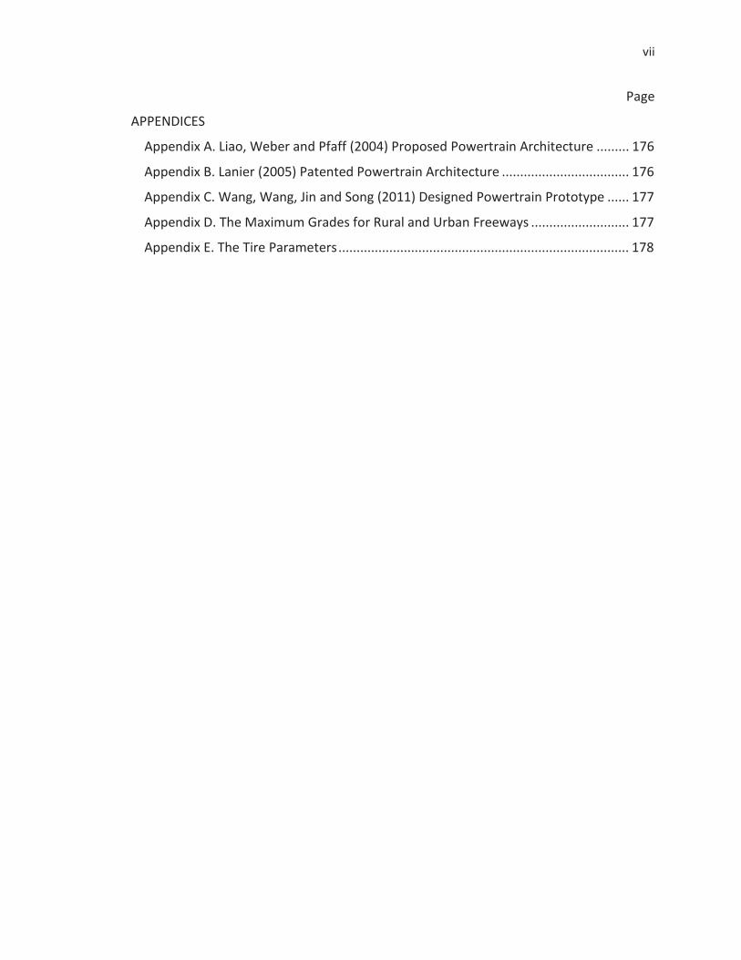
APPENDICES
Appendix A. Liao, Weber and Pfaff (2004) Proposed Powertrain Architecture ......... 176
Appendix B. Lanier (2005) Patented Powertrain Architecture ................................... 176
Appendix C. Wang, Wang, Jin and Song (2011) Designed Powertrain Prototype ...... 177
Appendix D. The Maximum Grades for Rural and Urban Freeways ........................... 177
Appendix E. The Tire Parameters ................................................................................ 178
viii
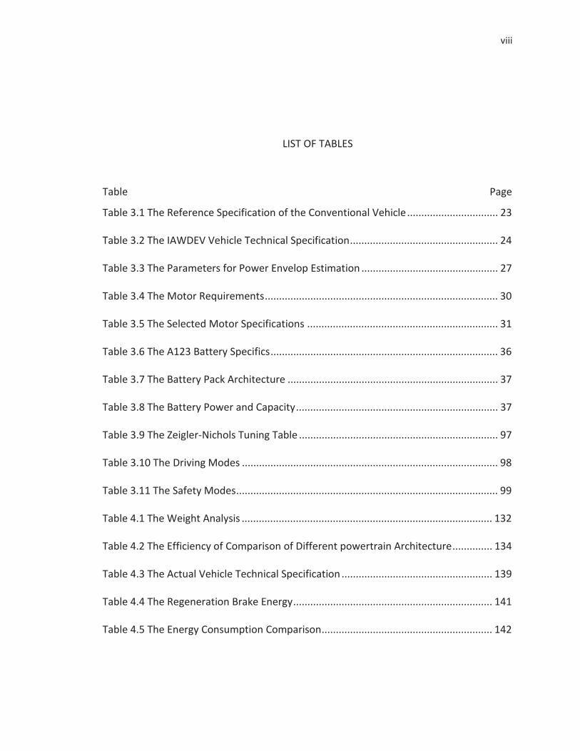
LIST OF TABLES
Table ...............................................................................................................................Page
Table 3.1 The Reference Specification of the Conventional Vehicle ................................ 23
Table 3.2 The IAWDEV Vehicle Technical Specification .................................................... 24
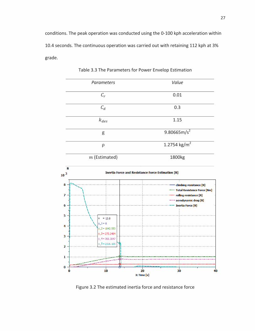
Table 3.3 The Parameters for Power Envelop Estimation ................................................ 27
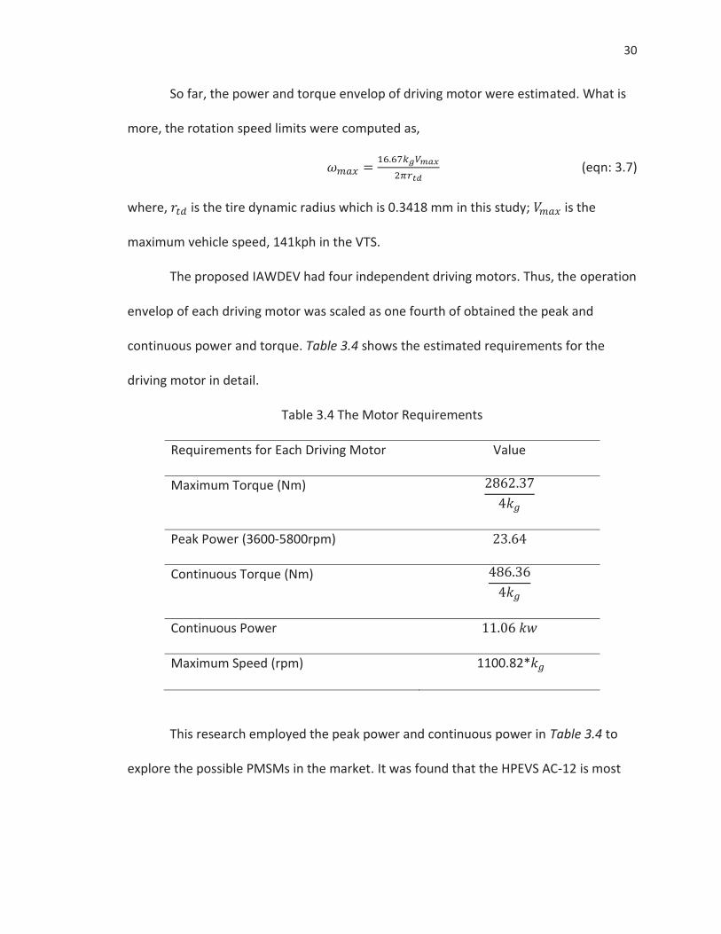
Table 3.4 The Motor Requirements .................................................................................. 30
Table 3.5 The Selected Motor Specifications ................................................................... 31
Table 3.6 The A123 Battery Specifics ................................................................................ 36
Table 3.7 The Battery Pack Architecture .......................................................................... 37
Table 3.8 The Battery Power and Capacity ....................................................................... 37
Table 3.9 The Zeigler-Nichols Tuning Table ...................................................................... 97
Table 3.10 The Driving Modes .......................................................................................... 98
Table 3.11 The Safety Modes ............................................................................................ 99
Table 4.1 The Weight Analysis ........................................................................................ 132
Table 4.2 The Efficiency of Comparison of Different powertrain Architecture .............. 134
Table 4.3 The Actual Vehicle Technical Specification ..................................................... 139
Table 4.4 The Regeneration Brake Energy ...................................................................... 141
Table 4.5 The Energy Consumption Comparison ............................................................ 142
ix
Table ...............................................................................................................................Page
Table 4.6 The Parameters of PI Controllers .................................................................... 149
Table 4.7 The Dimension Specifications of the Double-lane Change ............................. 161
x
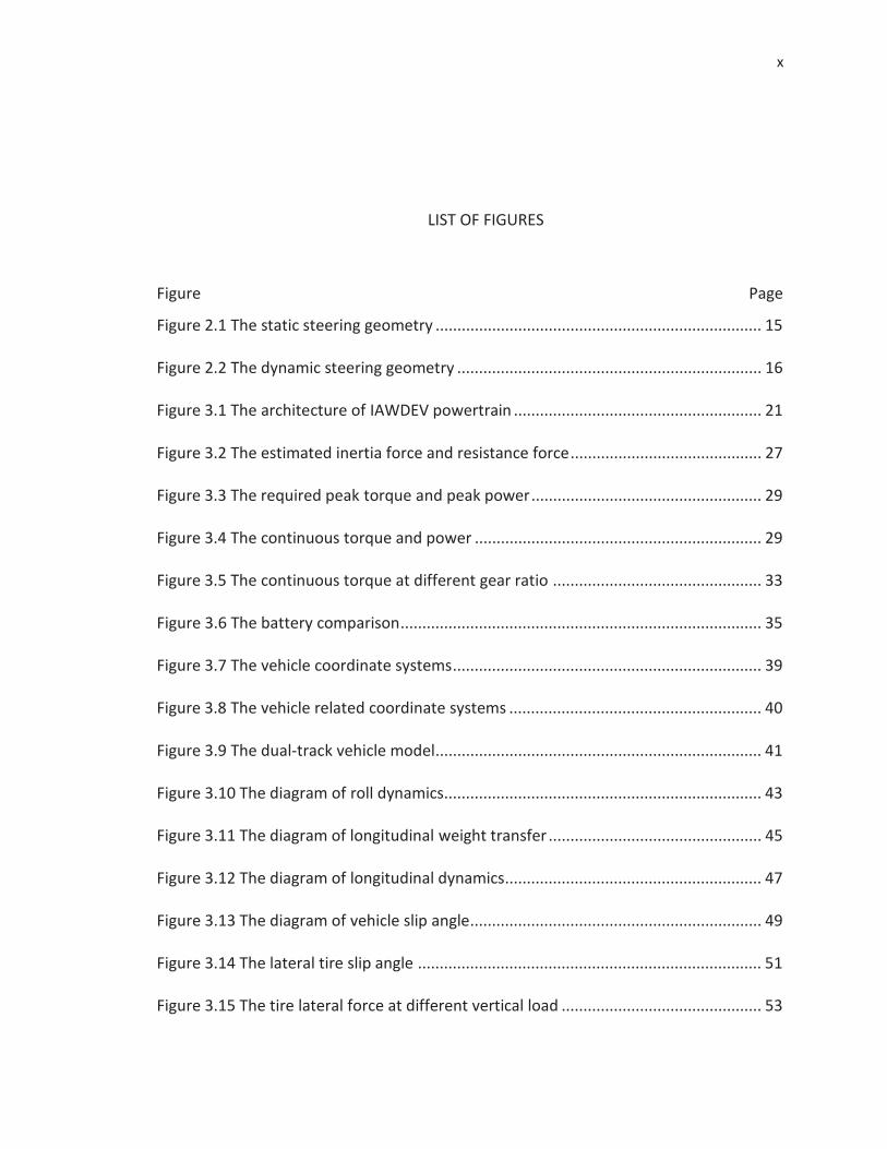
LIST OF FIGURES
Figure .............................................................................................................................Page
Figure 2.1 The static steering geometry ........................................................................... 15
Figure 2.2 The dynamic steering geometry ...................................................................... 16
Figure 3.1 The architecture of IAWDEV powertrain ......................................................... 21
Figure 3.2 The estimated inertia force and resistance force ............................................ 27
Figure 3.3 The required peak torque and peak power ..................................................... 29
Figure 3.4 The continuous torque and power .................................................................. 29
Figure 3.5 The continuous torque at different gear ratio ................................................ 33
Figure 3.6 The battery comparison ................................................................................... 35
Figure 3.7 The vehicle coordinate systems ....................................................................... 39
Figure 3.8 The vehicle related coordinate systems .......................................................... 40
Figure 3.9 The dual-track vehicle model ........................................................................... 41
Figure 3.10 The diagram of roll dynamics ......................................................................... 43
Figure 3.11 The diagram of longitudinal weight transfer ................................................. 45
Figure 3.12 The diagram of longitudinal dynamics ........................................................... 47
Figure 3.13 The diagram of vehicle slip angle ................................................................... 49
Figure 3.14 The lateral tire slip angle ............................................................................... 51
Figure 3.15 The tire lateral force at different vertical load .............................................. 53
xi
Figure .............................................................................................................................Page
Figure 3.16 The geometric relationship during the vehicle cornering ............................. 55
Figure 3.17 The coordinate transformation ..................................................................... 62
Figure 3.18 The intermediate coordinate system ............................................................ 65
Figure 3.19 The battery schematic ................................................................................... 70
Figure 3.20 The control system architecture .................................................................... 76
Figure 3.21 The driver reaction time ................................................................................ 78
Figure 3.22 The extended data frame of CAN bus ............................................................ 78
Figure 3.23 The motor control scheme ............................................................................ 87
Figure 3.24 The dual-loop control diagram ...................................................................... 88
Figure 3.25 The model of the PI controller ....................................................................... 89
Figure 3.26 The model of the motor plant ....................................................................... 90
Figure 3.27 The motion model of the motor .................................................................... 91
Figure 3.28 The model of the current loop ....................................................................... 92
Figure 3.29 The model of the speed loop ......................................................................... 93
Figure 3.30 The transformation of the s-plane and z-plane ............................................. 95
Figure 3.31 The transformation of the primary pole ........................................................ 96
Figure 3.32 The pedal control scheme ........................................................................... 101
Figure 3.33 The N-S chart of traction and brake control ................................................ 103
Figure 3.34 The Dugoff’s tire longitudinal force characteristics ..................................... 105
Figure 3.35 The diagram of the sliding mode control .................................................... 107
Figure 3.36 The N-S chart of the differential control ..................................................... 112
xii
Figure .............................................................................................................................Page
Figure 3.37 The state chart of the differential control ................................................... 113
Figure 3.38 The framework of the neural network predictive control........................... 116
Figure 3.39 The architecture of the neural network ...................................................... 117
Figure 3.40 The V-cycle diagram ..................................................................................... 124
Figure 3.41 The verification scheme of the motor control ............................................. 125
Figure 3.42 The verification scheme of the powertrain controller ................................ 126
Figure 3.43 The hard ware in the loop architecture ....................................................... 128
Figure 4.1 The weight comparison chart ........................................................................ 133
Figure 4.2 The acceleration performance ....................................................................... 135
Figure 4.3 The braking performance .............................................................................. 136
Figure 4.4 The cruising performance at 3% grade .......................................................... 137
Figure 4.5 The vehicle range at Max. vehicle speed and 112kph ................................... 138
Figure 4.6 The analysis of NEDC trace and SOC .............................................................. 140
Figure 4.7 The regeneration brake of the NEDC ............................................................. 141
Figure 4.8 The HWFET driving cycle ................................................................................ 142
Figure 4.9 The regeneration brake energy ..................................................................... 143
Figure 4.10 The step response of the current loop ........................................................ 144
Figure 4.11 The root locus of the closed current loop ................................................... 145
Figure 4.12 The disturbance rejection of the closed current loop ................................. 146
Figure 4.13 The step response of the dual loop ............................................................. 146
Figure 4.14 The Bode analysis of the closed dual-loop .................................................. 147
xiii
Figure .............................................................................................................................Page
Figure 4.15 The root locus of the closed dual-loop ........................................................ 148
Figure 4.16 The disturbance rejection of the closed dual-loop ...................................... 149
Figure 4.17 The Bode analysis of the feed-forward control ........................................... 150
Figure 4.18 The step response of the feed-forward control .......................................... 150
Figure 4.19 The SOC depleting comparison of mode controls ....................................... 152
Figure 4.20 The performance of the slipping control ..................................................... 153
Figure 4.21 The torque profile of the slipping control ................................................... 154
Figure 4.22 The slipping performance during US06 test ................................................ 154
Figure 4.23 The oversteering torque profile ................................................................... 156
Figure 4.24 The driving torque difference profile .......................................................... 156
Figure 4.25 The oversteering torque under the differential control .............................. 157
Figure 4.26 The regression plot ...................................................................................... 158
Figure 4.27 The comparison between the NNPM and plant output .............................. 159
Figure 4.28 The network training performance ............................................................. 160
Figure 4.29 The gradient profile ..................................................................................... 160
Figure 4.30 The routine of the double-lane change test ................................................ 161
Figure 4.31 The steering angle profile ............................................................................ 162
Figure 4.32 The yaw rate profile of the double-lane change test .................................. 163
xiv
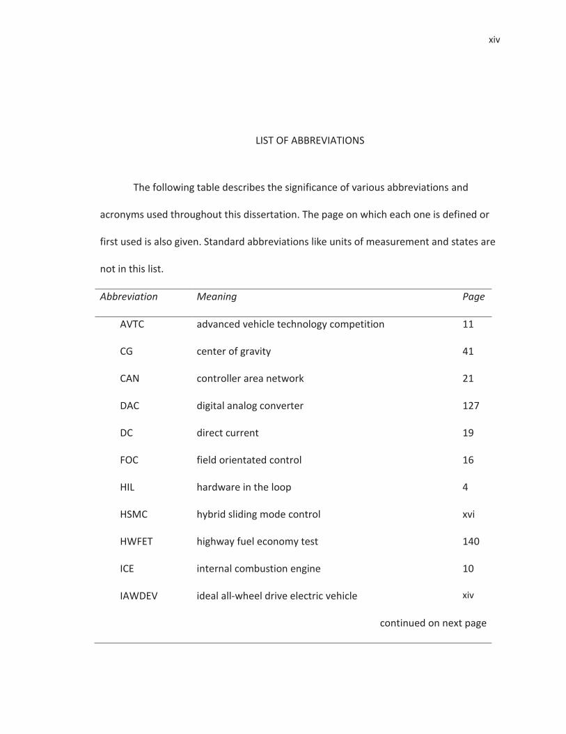
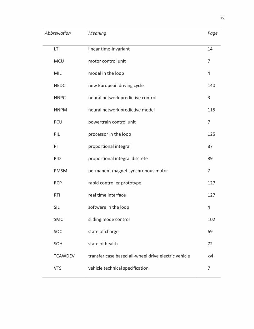
LIST OF ABBREVIATIONS
The following table describes the significance of various abbreviations and
acronyms used throughout this dissertation. The page on which each one is defined or
first used is also given. Standard abbreviations like units of measurement and states are
not in this list.
Abbreviation Meaning Page
AVTC advanced vehicle technology competition 11
CG center of gravity 41
CAN controller area network 21
DAC digital analog converter 127
DC direct current 19
FOC field orientated control 16
HIL hardware in the loop 4
HSMC hybrid sliding mode control xvi
HWFET highway fuel economy test 140
ICE internal combustion engine 10
IAWDEV ideal all-wheel drive electric vehicle xiv
continued on next page
xv
Abbreviation Meaning Page
LTI linear time-invariant 14
MCU motor control unit 7
MIL model in the loop 4
NEDC new European driving cycle 140
NNPC neural network predictive control 3
NNPM neural network predictive model 115
PCU powertrain control unit 7
PIL processor in the loop 125
PI proportional integral 87
PID proportional integral discrete 89
PMSM permanent magnet synchronous motor 7
RCP rapid controller prototype 127
RTI real time interface 127
SIL software in the loop 4
SMC sliding mode control 102
SOC state of charge 69
SOH state of health 72
TCAWDEV transfer case based all-wheel drive electric vehicle xvi
VTS vehicle technical specification 7
xvi
ABSTRACT
Wu, Haotian. Ph.D., Purdue University, December, 2014. Model-based Powertrain Design and Control System Development for the Ideal All-wheel Drive Electric Vehicle. Major Professor: Haiyan H. Zhang.
The transfer case based all-wheel drive electric vehicle (TCAWDEV) and dual-axle
AWDEV have been investigated to balance concerns about energy consumption,
drivability and stability of vehicles. However, the mentioned powertrain architectures
have the torque windup issue or the wheel skidding issue. The torque windup is an
inherent issue of mechanical linked all-wheel drive systems. The hydraulic motor-based
or the electric motor-based ideal all-wheel drive powertrain can provide feasible
solutions to the mentioned issues. An ideal AWDEV (IAWDEV) powertrain architecture
and its control schemes were proposed by this research; the architecture has four
independent driving motors in powertrain. The IAWDEV gives more control freedoms to
implement active torque controls and traction mode controls. In essence, this research
came up with the distributed powertrain concept, and developed control schemes of
the distributed powertrain to replace the transfer case and differential devices. The
study investigated the dual-loop motor control, the hybrid sliding mode control (HSMC)
and the neural network predictive control to reduce energy consumption and achieve
xvii
better drivability and stability by optimizing the torque allocation of each dependent
wheel. The mentioned control schemes were respectively developed for the anti-slip,
differential and yaw stability functionalities of the IAWDEV powertrain. This study also
investigated the sizing method that the battery capacity was estimated by using cruise
performance at 3% road grade. In addition, the model-based verification was employed
to evaluate the proposed powertrain design and control schemes. The verification
shows that the design and controls can fulfill drivability requirements and minimize the
existing issues, including torque windup and chattering of the slipping wheel. In
addition, the verification shows that the IAWDEV can harvest around two times more
energy while the vehicle is running on slippery roads than the TCAWDEV and the dual-
axle AWDEV; the traction control can achieve better drivability and lower energy
consumption than mentioned powertrains; the mode control can reduce 3% of battery
charge depleting during the highway driving test. It also provides compelling evidences
that the functionalities achieved by complicated and costly mechanical devices can be
carried out by control schemes of the IAWDEV; the active torque controls can solve the
inherent issues of mechanical linked powertrains; the sizing method is credible to
estimate the operation envelop of powertrain components, even though there is some
controllable over-sizing.
1
CHAPTER 1. INTRODUCTION
This chapter establishes the importance of this research, in contrast to existing
researches, and also examines the gap by summarizing a large amount of literature.
Moreover, the limitation and research questions are carefully outlined. Finally, the
dissertation organization is briefly introduced as a guideline for readers.
1.1 Overview
Reducing greenhouse gas emission, the reliance on the gasoline and energy
consumption and enhancing the drivability and safety are globally becoming the hot
concerns about vehicle technologies. In response to these concerns, alternative and
advanced powertrains are becoming an up to date research field in the auto industry
and research institutions. As a result, the leading automotive companies put a lot of
resources to improve of alternative powertrain architectures. The known powertrain
architectures include the power split, parallel through the road, series, parallel, range
extender and pure electric. These architectures have been applied in several vehicle
models in the market or in a prototype build. Toyota released its first generation Prius
into the market in 1997; the Prius employed the power split architecture. GM lunched
the Volt using range extender architecture in 2008. Tesla released the model S into the
2
market in 2012. The model S has the high performance pure electric powertrain. These
in production powertrains are sole axle design. The control development of these
powertrains focuses on optimizing the energy consumption on descent condition roads.
By contrast, the drivability and safety concerns on icy and slippery road haven’t been a
strong motivation for industry.
However, sustainable and advanced powertrains should not be limited to the
energy consumption and emission reduction; one of these powertrains should provide
an option to achieve as good drivability as conventional all-wheel drive vehicles. All-
wheel drive can and should be used all the time in view of the fact that all-wheel drive
provides better tracking, has less tendency to wander and weave, nearly eliminates
oversteer and understeer, allows larger acceleration without spinning out and has a far
greater resistance to hydroplaning (Dick, 1995). The consumers are motivated by these
advantages; their motivation is to avoid getting stuck in foul weather and to enjoy the
best combination of handling and safety. The automotive industry has been dedicated
to implement the all-wheel drive by using various mechanical transfer cases. As a result
of these advantages, the all-wheel drive hybrid or electric powertrain is an essential
fraction alternative powertrains.
In order to fill the current technology absence, several studies have been
conducted on all-wheel drive hybrid, but few studies focused on understanding the
efficiency and weight impact of the IAWDEV powertrain and analyzing how the IAWDEV
control system allocating the torque at each wheel to achieve better functionalities than
the mechanical drivetrain. This research primarily aimed to implement the
3
functionalities of the all-wheel by optimizing the torque allocation of four independent
driving motors. The functionalities include the anti-slip, differential and yaw stability
controls.
1.2 Research Scope
In general, this research focused on the model-based design and the control
development of the IAWDEV. The functional integration of the powertrain is the central
scope of this research. The modeling of the components just supports the functional
integration purpose rather than the design of components. In other words, the motor
design, gear design, battery design, the powertrain structural design and the chassis
structural design aren’t included in this research. In addition, this research employed
the electrical drive system which has lower voltage but higher current. The research was
conducted under the assumption that the superconducting material has achieved
significant advances. This research didn’t investigate how the superconducting material
is designed.
This research firstly proposed methods to design and size the powertrain
components, and systematically presented the modeling of IAWDEV. In detail, the dual-
track model of vehicle dynamics, the model of steering geometry, the non-linear model
of tires and the model of electric drive systems were carefully investigated. Secondly,
the active anti-slip control on accelerating and braking was developed; the differential
function was designed using the speed and torque control of driving motors; the neural
network predictive controller (NNPC) was investigated to maintain the yaw stability with
4
minimum energy consumption. By contrast, the yaw stability, the roll stability and pitch
stability strongly interacted with the active suspension design which is not the focus of
this research. The suspension links were assumed as rigid rods. Therefore, the roll
dynamics in this study was just used for the weight transfer analysis. Similarly, the shafts
were assumed to be absolutely rigid. On the basis of this assumption, the shafts had no
strain. Moreover, the verification of the proposed IAWDEV and its controls were also
conducted using the model in the loop (MIL), software in the loop (SIL) and hardware in
the loop (HIL) technologies. This research wasn’t investigated how the technologies
were developed by vendors.
1.3 Research Questions
The questions central to this research were:
1. Whether does the IAWDEV have a significant weight increase and lower
efficient in contrast to the traditional powertrains?
2. How is the IAWDEV sized to meet the vehicle technical specification?
3. How are the anti-slip, differential and yaw stability functionalities achieved
by just using control schemes?
4. Whether the integrated control system can assist the vehicle to recover from
the un-steady cornering?
1.4 Limitations
The following limitations were inherent to the pursuit of this research:
5
1. It is not feasible to carry out the prototype build and conduct the experiment
on proving grounds due to the costly and complex hardware requirements.
2. This research was limited to the computational accuracy of the models and
the computational performance of the simulation solver.
3. This study was limited to the tremendous complexity of the tire physical
model.
1.5 Delimitations
In order to minimize the negative effect of the above limitations, the following
delimitations were used to pursue this study:
First, this research fully took advantage of the facilities available at Purdue
University. This study employed the Co-simulation technology of AMEsim and Carsim.
By using the Co-simulation technology of AMEsim, the experimentally proved lithium-
ion battery, permanent magnet synchronous motor and inverter functioned as the
prototype platform of electric drive system. By utilizing the Carsim, the most accurate
methods were provided to evaluate vehicle dynamic performance; these methods can
provide reasonable results in comparison. In addition, the technology of MIL, SIL and HIL
was carefully employed to verify the powertrain design and the control system.
Second, the workstation in the Multiple Disciplinary Lab was employed. The
parallel computing toolbox of Matlab was also used to speed up the neural network
training process.
6
Third, to avoid this unnecessary complexity, the multivariate regression model,
Dugoff’s tire model, was employed to accurately estimate the tire model.
1.6 Organization
The dissertation mainly consists of the introduction section, methodology section,
results section and conclusion section. In each section, there are several sub-sections.
Chapter1 introduces the overview of this research and briefly summarized the
previous research studies. On the basis of these reviews, the general concerns about
hybrid and electric vehicle powertrain are discussed. The further discussion eventually
narrows down the research scope to the design of IAWDEV and its controls in a
systematic manner. In addition, the research questions, limitations and delimitations are
also specified in the independent sub-sections.
In chapter 2, the principal literature is reviewed. The history of all-wheel drive
system for conventional vehicles is summarized in the first place. In the sequel, all-
wheel drive of electrified powertrains is introduced. The models of powertrain and
vehicle dynamics play essential role in the control development. This study thus reviews
a large amount of previous studies to highlight the possible gap and the innovation
which this research should focus on. Moreover, the motor and Powertrain controls are
outlined to point out the difference between the previous and current studies.
In chapter 3, the powertrain architecture is firstly presented as an overview of this
section. Then, the specific powertrain component and parameters are selected and
sized. In the second place, powertrain modeling is discussed. The vehicle dynamics and
7
Powertrain modeling are the foundation of model-based development. For the sake of
control development, vehicle dynamics and electric drive system are carefully modeled.
The generic vehicle dynamic models cover yaw dynamics, roll dynamics, longitudinal
dynamics, weight transfer, slip angles and steering angles. The generic vehicle electric
drive system models include the Li-ion battery model and the model of permanent
magnet synchronous motor (PMSM). The complete electric drive assemble is simulated
in AMEsim to obtain high fidelity simulation data. With the models and obtained data,
the development of controllers is conducted. For the real-time application, the sample
rate is critical. Therefore, the timer configuration is firstly described. On the basis of the
discrete models and timer configuration, the MCU and the PCU are designed and
analyzed in detail. Also, the verification methods of the proposed control laws are
summarized at the end.
Chapter 4 reports the results of the verifications of the powertrain design and the
control performance. Firstly, the weight analysis, the verification of the vehicle technical
specification (VTS) and driving cycle test are discussed. Secondly, the control system is
integrated with the powertrain of the IAWDEV; then, the slipping control, differential
control and yaw stability control are verified.
Chapter 5 provides the conclusions of the study, and discussion of the results and
recommendations for further research.
8
1.7 Summary
This chapter offered an initiation to the research, including overview, literature
review, research scope, research questions, limitations and delimitation. The next
chapter presents the powertrain architecture design, powertrain modeling and
controller development in detail.
9
CHAPTER 2. LITERATURE REVIEW
The all-wheel drive concept has a long history. The all-wheel drive device for
conventional vehicles was patented by Zachow and Besserdich as early as 1908. Since
then, studies have been conducted to develop more efficient all-wheel drive system. As
the advance of powertrain electrification, the AWDEV continues to be a hot topic
throughout the powertrain design and control. This chapter outlines previous studies on
the design of powertrain architectures, the modeling of the vehicle and tire dynamics,
the motor and powertrain controls.
2.1 Powertrain Architecture
The better mobility has been continuously pursued since the early stage of
motorized vehicle. The all-wheel drive concept thus has a long history of the
conventional vehicle. Zachow and Besserdich (1908) patented a power-applying
mechanism. In fact, the mechanism aimed to factor the driving power between the
front and rear axles. In the sequel, a four-wheel drive vehicle construction was discussed
in Kingsley (1931). As the energy efficiency and drivetrain noise are becoming a
highlighted concern, a selectively engageable transfer case was investigated by
Sampietro and Matthews (1965). The selectively engageable design eventually evolved
10
to the automatic four-wheel drive transfer case in Fogelberg (1976). As noted, above
remarkable inventions are mechanically linked and designated to the conventional
powertrain in which primary components are the internal combustion engine (ICE) and
the transmission. The mentioned mechanical devices did achieve functionalities of all-
wheel drive. As described by Dick (1995), the mechanical transfer case causes the
torque windup while the all-wheel drive vehicle is cornering. During the vehicle
cornering, each wheel goes though different trace and has different wheel speed. Thus,
the lock-up transfer case results in the torque windup and gear noise. By contrast, the
automatic transfer case temporarily disengages a driving axle to eliminate the torque
windup, which implies that the vehicle loses all-wheel mobility while cornering.
In order to solve the discussed problems, the ideal all-wheel drive powertrain
was preferred. The ideal all-wheel drive system provides continuous variant torque at
each wheel as required by performance objectives (Dick, 1995). For the sake of this goal,
a hydraulic drive or a continuously variable mechanical drive can be applied to each
wheel. The hydraulic drive prototype is more preferred for heavy duty vehicles, such as
agricultural and mining vehicles. The continuously variable mechanical drive is almost
impossible to use the ICE due to its packaging difficulty, whereas is feasible to employ
electric drive. This study thus proposed an ideal all-wheel drive electric vehicle
powertrain has no mechanical connection between each wheel and eliminate the
transfer case, the inter-wheel and inter-axle differentials. These offer possibilities to
reduce powertrain weight and cost and to increase the control freedom to implement
the slip control, differential control and stability control.
11
Moreover, as the continuous growth of hybrid vehicles and electric vehicles, a
large amount of studies have also been projected on the all-wheel drive for the
electrified powertrain. Liao, Weber and Pfaff (2004) described a concept of strong
hybridization powertrain on all-wheel drive sport utility vehicles. In their design, the
conventional gas engine was retained at the rear axle; a boost motor was added to the
front axle. The architecture is presented in Appendix A; it is very similar to the
mentioned parallel-through-the-road design. Liao, Weber and Pfaff (2004) also
introduced strong hybrid powertrains on all-wheel drive sport utility vehicles, in which
the all-wheel drive based on a mechanical transfer case. Lanier (2005) filed an all-wheel
drive electric vehicle patent. In his innovation, an electric motor replaces the gas engine
to power four wheels through a transfer case and axle differentials as shown in
Appendix B. The configuration does minimize the adjustment to the traditional all-wheel
drive. The cost is that space for battery system is heavily occupied by drivetrain
components. Thus, the passenger capacity is eventually reduced. This architecture also
has inherent drawbacks of the mechanical transfer case.
Thus, the parallel-through-the-road hybrid gradually becomes a hot thread. This
concept was deeply researched by several universities which were getting involved in
the Challenge X or EcoCar project under Advanced Vehicle Technology Competition
(AVTC) platform. The Mississippi State University team transformed Chevrolet Equinox
into a diesel-electric hybrid vehicle for Challenge X in Young et al. (2007). The Ohio State
University Challenge X team presented the implementation of an electric all-wheel drive
system on a power split vehicle, parallel-through-the-road hybrid electric vehicle (Arnett,
12
Rizzoni, & Heydinger, 2008). The Purdue University EcoCar2 team converted a
conventional Malibu into a bio-diesel hybrid in 2012 (Wu et.al., 2013). All three teams
employed the parallel through the road concept; Mississippi State University and Ohio
State University applied this concept to a truck and Purdue University adapted to it to a
full size sedan. The parallel-through-the-road hybrid is a mechanically independent
powertrain between the fore and aft axle; without mechanical link, the axles are
coupled through road surface and the fore and aft tires. This architecture makes the
continuously variable torque distribution feasible and nearly solves the torque windup
issue. On the other hand, it has some disadvantages on account of that it only use one
axle to harvest braking energy.
The IAWDEV based on gearless in-wheel motors therefore lies in the researchers’
scope. Rahman et al. (2006) investigated an in-wheel motor based on the axial flux
permanent magnet motor. Li, Wu, Zhang and Gao (2010) presented a vernier in-wheel
motor which meet the weight, size and torque requirements of electric vehicles. As
significant advance in the in-wheel motor, Wang, Chen, Feng, Huang, and Wang (2011)
set up a prototyping AWDEV which is similar to a golf cart. The prototype employed four
independent in-wheel motors and the 72 V lithium-ion battery pack. The researchers
initiated the detailed presentation of the design and performance analysis for the
IAWDEV using four in-wheel motors.
The main difference between the proposed architecture and those discussed
earlier lies in the motor drive and the battery pack. This study utilized four independent
PMSMs, which are mounted to the chassis frame rather than the wheel hub. It implies
13
that the proposed architecture eliminated the large unsprang mass of the in-wheel
motor; it is more suitable for passenger cars. In addition, this study used a 144 V high
performance lithium-ion pack, which obtains larger power with relatively small current.
2.2 Model-based Design
Obviously, the model of the system should be highlighted as the foundation of
the model-based design. The modeling in this research also serves as the baseline of
control development. The modeling covers vehicle dynamics, tire dynamics, steering
geometry and electric drive systems.
2.2.1 Vehicle and Tire Dynamics
As a continuous hot topic, previous researchers have devoted tremendous
efforts into studies on vehicle dynamics. Gillespie (1992) systematically introduced the
acceleration, brake, ride and steady-state cornering performances of passenger cars and
light trucks. Millken and Millken (1995) discussed aerodynamics, vehicle axis systems,
steady-state stabilities and designs of race cars. Both studies gave very detailed
explanation of vehicle dynamics; they are the foundations of the modern vehicle
dynamics. This study cited some ideas in above two studies. The innovation of this study
should be noted as this study developed the dual-track model rather than the signal
track model.
In order to achieve the differential and stability controls, the dual track model is
essential for the IAWDEV. The dual-track model of the yaw motion in Esmailzadeh,
14
Vossoughi and Goodarzi (2001) and Zhao, Zhang and Zhao (2009) included both lateral
and longitudinal forces on the left and right tracks. However, the model neglected the
impact of the lateral slip angles of tires. By contrast, this study didn’t only apply the
dual-track model on the basis of previous studies, but also took the lateral slip angles of
tires into account. Wang, Zhang and Wang (2013) developed the dual-track model of
yaw dynamics that considers the significant impact of the lateral slip angles of tires. The
model in Wang, Zhang and Wang (2013) is credible for the steady-state cornering, but is
not suitable for the unsteady-state cornering. The reason is that the model in Wang,
Zhang and Wang (2013) neglected the load transfer of each wheel. For the unsteady-
state cornering such as wheel slipping, the normal load of the tire has a significant
impact on the driving force, which directly affects the yaw stability control. This study
added the load transfer at each wheel into the dual-track model of yaw and longitudinal
dynamics. In addition, the Dugoff’s tire model was employed to investigate how the load
transfer affects the yaw and longitudinal dynamics.
Taking a further review of previous researches, it was found that these
researches simplified the system model as the linear time-invariant (LTI) and continuous
system problems, whereas most of digital controller cannot process data continuously in
Ellis (2004). To the author’s knowledge, a complete research on the discrete modeling
and control development of IAWDEV remains unstudied.
15
2.2.2 Steering Geometry
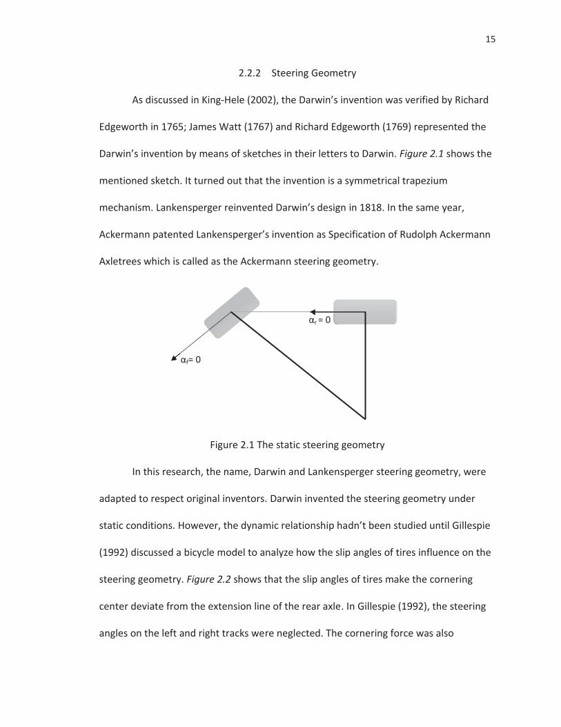
As discussed in King-Hele (2002), the Darwin’s invention was verified by Richard
Edgeworth in 1765; James Watt (1767) and Richard Edgeworth (1769) represented the
Darwin’s invention by means of sketches in their letters to Darwin. Figure 2.1 shows the
mentioned sketch. It turned out that the invention is a symmetrical trapezium
mechanism. Lankensperger reinvented Darwin’s design in 1818. In the same year,
Ackermann patented Lankensperger’s invention as Specification of Rudolph Ackermann
Axletrees which is called as the Ackermann steering geometry.
Figure 2.1 The static steering geometry
In this research, the name, Darwin and Lankensperger steering geometry, were
adapted to respect original inventors. Darwin invented the steering geometry under
static conditions. However, the dynamic relationship hadn’t been studied until Gillespie
(1992) discussed a bicycle model to analyze how the slip angles of tires influence on the
steering geometry. Figure 2.2 shows that the slip angles of tires make the cornering
center deviate from the extension line of the rear axle. In Gillespie (1992), the steering
angles on the left and right tracks were neglected. The cornering force was also
αr = 0
αf= 0
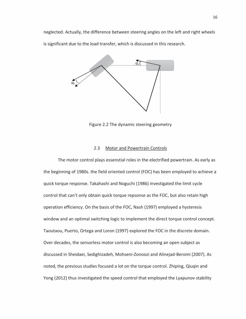
16
neglected. Actually, the difference between steering angles on the left and right wheels
is significant due to the load transfer, which is discussed in this research.
Figure 2.2 The dynamic steering geometry
2.3 Motor and Powertrain Controls
The motor control plays essenstial roles in the electrified powertrain. As early as
the beginning of 1980s. the field oriented control (FOC) has been employed to achieve a
quick torque response. Takahashi and Noguchi (1986) investigated the limit cycle
control that can’t only obtain quick torque repsonse as the FOC, but also retain high
operation efficiency. On the basis of the FOC, Nash (1997) employed a hysteresis
window and an optimal switching logic to implement the direct torque control concept.
Taoutaou, Puerto, Ortega and Loron (1997) explored the FOC in the discrete domain.
Over decades, the sensorless motor control is also becoming an open subject as
discussed in Sheidaei, Sedighizadeh, Mohseni-Zonoozi and Alinejad-Beromi (2007). As
noted, the previous studies focused a lot on the torque control. Zhiping, Qiuqin and
Yong (2012) thus investigated the speed control that employed the Lyapunov stability
αf
αr
17
criterion and the FOC. Based on the principle of the FOC, this study explored both
torque and speed control by using the dual-loop and feed-forward controls.
Besides the motor control, the powertrain control is indispensable to achieve the
functionalities of vehicles. For the centralized powertrain, the powertrain control
heavily relies on the engine, transmission, transfer case and active differential controls.
For the distributed powertrain like the proposed IAWDEV, it provides accessible ways to
portion the torque of each driving wheel. By reviewing the research history about the
IAWDEV control, it was found that previous researchers tremendously focused on the
yaw moment and steering controls. The most of earlier researchers described the fault-
tolerant control, the yaw control and the longitudinal velocity estimation for the in-
wheel-motor-based IAWDEV. A couple of researchers mentioned wheel slip and
differential controls for other powertrains instead of the IAWDEV. To the author’s best
knowledge, this research first investigated the design of the traction mode, anti-slip,
differential and yaw stability controls in a systematic manner. The difference between
this research and previous research is that this research achieved the anti-lock braking
based on the HSMC, and optimized the yaw stability based on the NNPC. It should be
the neural network was trained using a nonlinear training rate, which is significantly
different from the previous studies. The detailed reviews were outlined as follows.
Tahami et al. (2004) developed a fuzzy controller that allocates the torque of
each driving wheel; the controller eventually maintains the yaw rate in the reference
value. Mutoh and Yahagi (2005) introduced the electric braking control that allocates
the braking torque of the front and rear axles. The braking control was verified through
18
an in-wheel IAWDEV. Goodari and Esmailzadeh (2007) designed an innovative fuzzy
algorithm that portions the torque at each in-wheel motor to achieve a better yaw
response, and also limit the wheel slip within the optimal region. Goodari and
Esmailzadeh (2007) discussed the if-else rules that make a trade-off between the yaw
response and the wheel slip. However, they significantly simplified the longitudinal
dynamics as a pure linear model, which is deviated from the physical scenario. This is a
noticeable gap that this research was working on.
Moreover, Gao, Yu and Xu (2008) proposed a slip ratio control method using
fuzzy dynamical sliding mode strategy for the traction control. Magallan, Angelo,
Bisheirmer and Garcia (2008) carried out an electronic differential control by using two
independent induction motors in the front axle. Li, Wang and Liu (2008) investigated the
motor-torque-based yaw moment control for a four-wheel-drive electric vehicle using
fuzzy logic control method. Gao et al. (2008) presented a fuzzy logic based observer to
estimate the longitudinal velocity of a four-wheel-drive electric vehicle. Kada, Hartani &
Bourahla (2009) studied an electronic differential by using direct torque fuzzy control for
each rear-motor. Geng and Mostefai (2009) described a stabilizing observer-based
control algorithm for an in-wheel-motored vehicle to compensate yaw state deviation.
In addition, K Hartani, Miloud, & Miloudi (2010) developed the direct torque
controller of two independent driving motors to achieve the electronic differential
function. Wang, Wang, Jin and Song (2011) discussed the torque control of the IAWDEV
based on the in-wheel motor. The torque control assisted steering system to obtain
better steering returnability and retain the vehicle stability. The prototyping vehicle is
19
shown in Appendix C. Draou (2013) presented a simple sliding mode control strategy
used in an electronic differential system with two independent driving wheels in the
rear axle. Ravi & Palani (2013) proposed a robust control scheme of electronic
differential system for an electric vehicle with two brushless direct current (DC) motors.
2.4 Summary
This chapter has summarized the literature related to the powertrain design and
control development for the IAWDEV. It was carefully outlined a large amount of
researches about the Powertrain architecture, vehicle dynamics, the steering geometry,
the motor and Powertrain controls. To the author’s knowledge, the review of the
literature confirmed the significance of the questions claimed in this study. There seems
no literature attempt to answer the questions in a systematic manner.
20
CHAPTER 3. METHODOLOGY
In this section, the powertrain architecture is firstly discussed. In the sequel,
components of the proposed powertrain are specified and sized. On the basis of
specified components and parameters, the powertrain modeling is presented. The
powertrain modeling includes the vehicle dynamics and the electric drive system. Based
on models of the vehicle dynamics and the electric drive system, the control system of
the discussed powertrain is carefully developed. The control system consists of a low
level controller and a high level controller. The low level controller is the motor control
unit (MCU). The high level controller is the powertrain control unit (PCU) that covers the
slip control, the differential control and the yaw stability control. In order to closely
follow the development cycle of the automotive software, this research also
investigates verification methods of the discussed controllers. The verification methods
include the MIL, SIL and HIL.
3.1 Powertrain Architecture Design
This subsection illustrates the IAWDEV architecture in the first place. In the
sequel, the VTS is defined. Finally, the components for the IAWDEV are selected and
sized on the basis of the VTS.
21
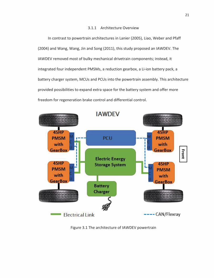
3.1.1 Architecture Overview
In contrast to powertrain architectures in Lanier (2005), Liao, Weber and Pfaff
(2004) and Wang, Wang, Jin and Song (2011), this study proposed an IAWDEV. The
IAWDEV removed most of bulky mechanical drivetrain components; instead, it
integrated four independent PMSMs, a reduction gearbox, a Li-ion battery pack, a
battery charger system, MCUs and PCUs into the powertrain assembly. This architecture
provided possibilities to expand extra space for the battery system and offer more
freedom for regeneration brake control and differential control.
Figure 3.1 The architecture of IAWDEV powertrain
MCU
MCU
MCU
MCU
22
Figure 3.1 describes the powertrain architecture. Four 45HP PMSMs replace the
traditional gasoline engine and independently power four wheels. Each motor is
equipped with a planetary gearbox which is to reduce angular speed and multiply
torque to the driving wheel. It should be noticed that four sets of the motor drive are
mounted to the chassis frame rather than the wheel hub. The electrical energy storage
system primarily consists of 96kW Li-ion battery pack. On board charging system is
Brusa level one charger with 3.7 kW maximum charging power. The MCU and the PCU
are two essential controllers for the AWDEV powertrain. The controllers are interacting
through control area network (CAN). The PCU is the master controller for the entire
powertrain. It includes four primary functions: the traction mode control, slipping
control, differential control and yaw control. The MCU focuses on controlling the driving
motor to track the torque and speed command from the PCU and then feeds back the
estimated torque and the measured speed to the PCU. This architecture has the ability
to enhance vehicles stability and handling by manipulating the individual motor torque
among four driving wheels and to reduce energy consumption due to higher efficiency
and lighter weight of the drivetrain.
3.1.2 Vehicle Technical Specifications
The prerequisite of the components selection, system modeling and control
development is the vehicle technical specifications (VTS) of the proposed structure. In
view of the fact that there is neither a stock model nor a prototype vehicle in the
present market, the on-road test data is not available for this research. Consequently,
23
the VTS were in turn derived from high fidelity modeling and simulation of the IAWDEV.
In order to increase the fidelity of the model, this research selected a stock vehicle as
the design reference. By comparing several stock vehicles, it was found that Mitsubishi
2015 AWD Outlander fits this research goal due to its drivability, size, power and weight.
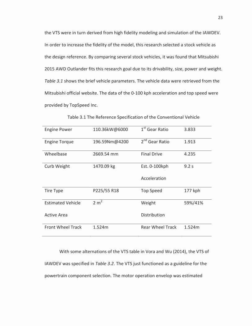
Table 3.1 shows the brief vehicle parameters. The vehicle data were retrieved from the
Mitsubishi official website. The data of the 0-100 kph acceleration and top speed were
provided by TopSpeed Inc.
Table 3.1 The Reference Specification of the Conventional Vehicle
Engine Power 110.36kW@6000 1st Gear Ratio 3.833
Engine Torque 196.59Nm@4200 2nd Gear Ratio 1.913
Wheelbase 2669.54 mm Final Drive 4.235
Curb Weight 1470.09 kg Est. 0-100kph
Acceleration
9.2 s
Tire Type P225/55 R18 Top Speed 177 kph
Estimated Vehicle
Active Area
2 m2 Weight
Distribution
59%/41%
Front Wheel Track 1.524m Rear Wheel Track 1.524m
With some alternations of the VTS table in Vora and Wu (2014), the VTS of
IAWDEV was specified in Table 3.2. The VTS just functioned as a guideline for the
powertrain component selection. The motor operation envelop was estimated

24
according to requirements of the acceleration, gradeability and top speed. The actual
VTS could have a bit deviation after the components are finalized; it is presented in the
results section.
Table 3.2 The IAWDEV Vehicle Technical Specification
Function Expected Vehicle Technical
Specifications
Acceleration 0–100 kph ≤10.4 Sec
Acceleration 80–112 kph ≤6.4 Sec
Braking 100–0 kph ≤50.2 m
Duration with 3% Grades (112 kph) ≥45 minutes
Duration with 6% Grades (100 kph) ≥30 minutes
Vehicle Range ≥140 km
Top Speed ≥141 kph
3.1.3 Component Selection and Sizing
This section introduced which types of component were employed in the
IAWDEV and how the components were sized to meet the predefined VTS.
3.1.3.1 Motor
This study explored numerous investigations of electric drives from conventional
brush Direct Current (DC) motors to PMSMs. Chattopadhyay (1997) summarized that
25
brush DC motors have been the most popular choice for many industrial drives in spite
of its inherent drawbacks. The DC motor needs to convert the direct current to the
alternating current by using commutation devices, brushes and commutators. These
devices need expensive regular maintenance.
By contrast, the commutation processes are implemented using power
electronic components for the brushless DC motor. In essence, the brushless DC motor
is one of PMSMs. The PMSM has been widely recognized in industrial drives, because it
has no potentially troublesome of electrical contacts, brushes and commutators. Yang
and Chuang (2007) stated that permanent magnet machines involve low losses as they
require no excitation current. Toliyat (2008) also outlined that the permanent magnet
motor is one of the best choices for the EV propulsion system on account of its potential
high efficiency, high power factor, high power density and excellent flux weakening
capability.
The permanent magnetic motor has two-phase and three-phase configurations.
For the three-phase configuration, the minimal number of power electronic devices
required (Hanselman, 1994). Besides, the three-phase motor has one more degree of
freedom than the two-phase motor. This offers more room for potential drive schemes
and control technologies.
In addition, the three-phase PMSM has two types of winding connection, and Y.
This study employed the Y connection. The Y connection is one of the most popular
configurations. The Y doesn’t introduce the extra terminal, the neutral point, to the
three-phase bridge; its power supply is applied from line to line instead of from line to
26
neutral point. Consequently, the motor control and electrical design are further
simplified by using the Y connection.
In view of the advantages of the PMSM with the Y connection, this study
selected the three-phase PMSM as the vehicle propulsion equipment. Sequentially, the
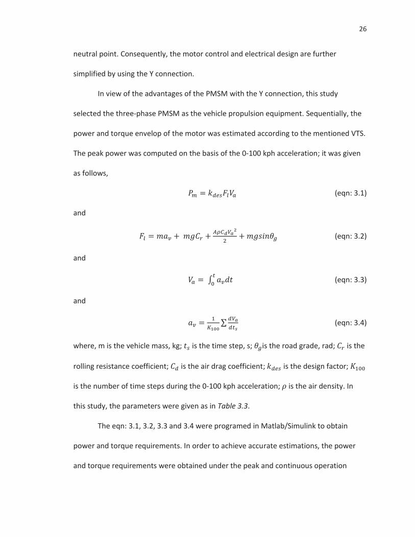
power and torque envelop of the motor was estimated according to the mentioned VTS.
The peak power was computed on the basis of the 0-100 kph acceleration; it was given
as follows,
(eqn: 3.1)
and
(eqn: 3.2)
and
(eqn: 3.3)
and
(eqn: 3.4)
where, m is the vehicle mass, kg; is the time step, s; is the road grade, rad; is the
rolling resistance coefficient; is the air drag coefficient; is the design factor;
is the number of time steps during the 0-100 kph acceleration; is the air density. In
this study, the parameters were given as in Table 3.3.
The eqn: 3.1, 3.2, 3.3 and 3.4 were programed in Matlab/Simulink to obtain
power and torque requirements. In order to achieve accurate estimations, the power
and torque requirements were obtained under the peak and continuous operation
27
conditions. The peak operation was conducted using the 0-100 kph acceleration within
10.4 seconds. The continuous operation was carried out with retaining 112 kph at 3%
grade.
Table 3.3 The Parameters for Power Envelop Estimation
Parameters Value
0.01
0.3
1.15
9.80665m/s2
1.2754 kg/m2
(Estimated) 1800kg
Figure 3.2 The estimated inertia force and resistance force
28
In order to obtain the load force, the 0-100 kph acceleration was conducted
under 0 road grade by simulating Eqn: 3.2. The resistance forces were presented in
Figure 3.2. Obviously, the inertia force is the dominant component during the vehicle
acceleration. The peak force was computed as 8237.762 N.
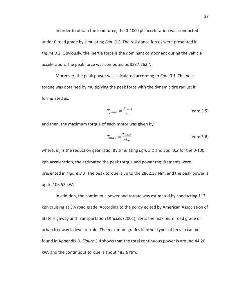
Moreover, the peak power was calculated according to Eqn: 3.1. The peak
torque was obtained by multiplying the peak force with the dynamic tire radius; it
formulated as,
(eqn: 3.5)
and then, the maximum torque of each motor was given by,
(eqn: 3.6)
where, is the reduction gear ratio. By simulating Eqn: 3.1 and Eqn: 3.2 for the 0-100
kph acceleration, the estimated the peak torque and power requirements were
presented in Figure 3.3. The peak torque is up to the 2862.37 Nm, and the peak power is
up to 106.52 kW.
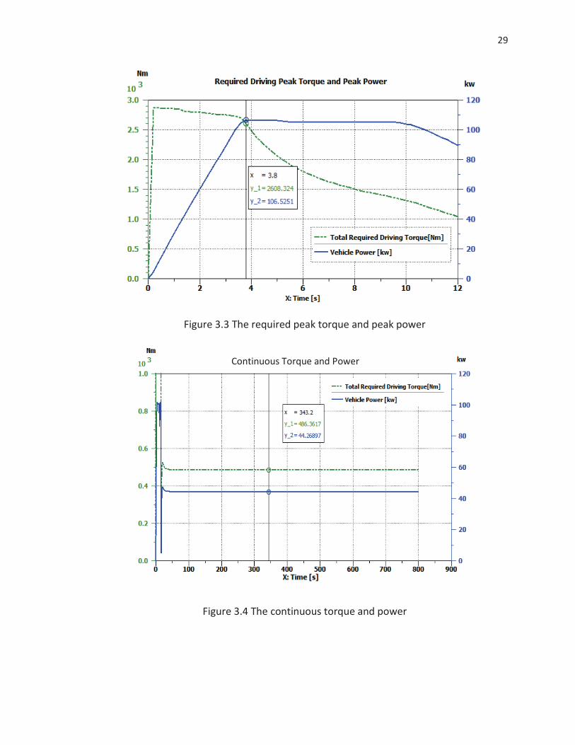
In addition, the continuous power and torque was estimated by conducting 112
kph cruising at 3% road grade. According to the policy edited by American Association of
State Highway and Transportation Officials (2001), 3% is the maximum road grade of
urban freeway in level terrain. The maximum grades in other types of terrain can be
found in Appendix D. Figure 3.4 shows that the total continuous power is around 44.26
kW, and the continuous torque is about 483.6 Nm.
29
Figure 3.3 The required peak torque and peak power
Figure 3.4 The continuous torque and power
Continuous Torque and Power
30
So far, the power and torque envelop of driving motor were estimated. What is
more, the rotation speed limits were computed as,
(eqn: 3.7)
where, is the tire dynamic radius which is 0.3418 mm in this study; is the
maximum vehicle speed, 141kph in the VTS.
The proposed IAWDEV had four independent driving motors. Thus, the operation
envelop of each driving motor was scaled as one fourth of obtained the peak and
continuous power and torque. Table 3.4 shows the estimated requirements for the
driving motor in detail.
Table 3.4 The Motor Requirements
Requirements for Each Driving Motor Value
Maximum Torque (Nm)
Peak Power (3600-5800rpm)
Continuous Torque (Nm)
Continuous Power
Maximum Speed (rpm) 1100.82*
This research employed the peak power and continuous power in Table 3.4 to
explore the possible PMSMs in the market. It was found that the HPEVS AC-12 is most
31
likely suitable to the obtained power envelop; the motor is produced by Hi Performance
Electric Vehicle Systems Inc.
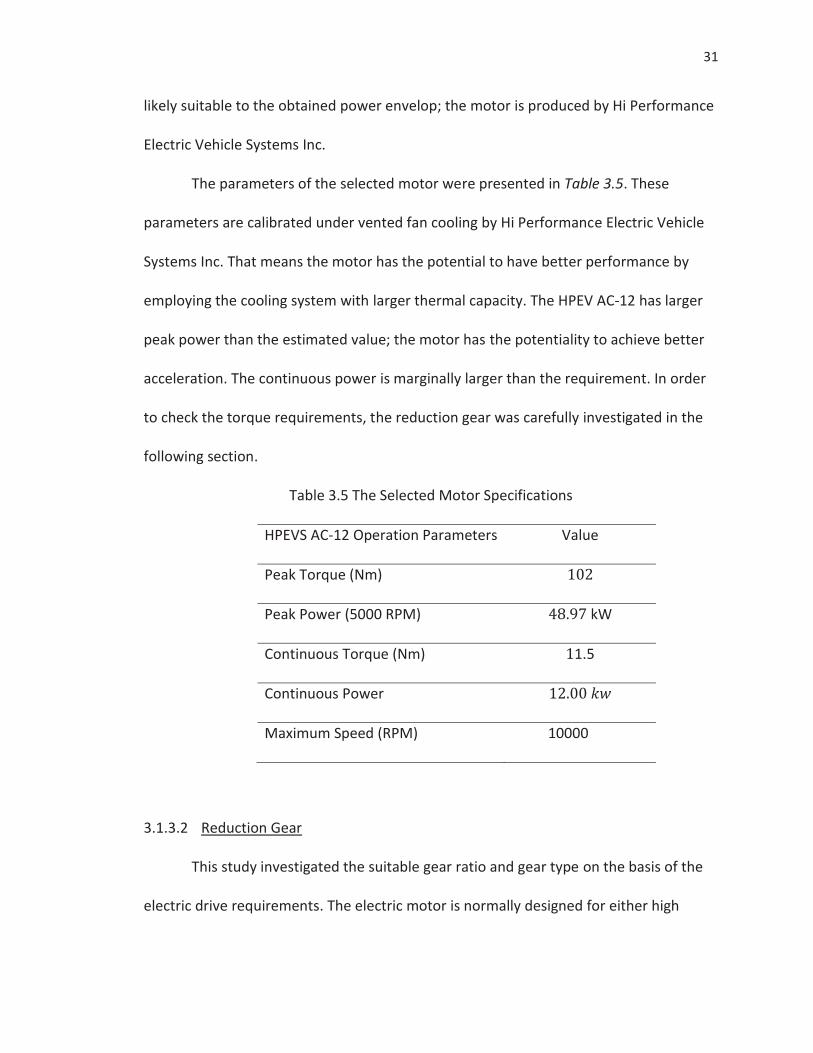
The parameters of the selected motor were presented in Table 3.5. These
parameters are calibrated under vented fan cooling by Hi Performance Electric Vehicle
Systems Inc. That means the motor has the potential to have better performance by
employing the cooling system with larger thermal capacity. The HPEV AC-12 has larger
peak power than the estimated value; the motor has the potentiality to achieve better
acceleration. The continuous power is marginally larger than the requirement. In order
to check the torque requirements, the reduction gear was carefully investigated in the
following section.
Table 3.5 The Selected Motor Specifications
HPEVS AC-12 Operation Parameters Value
Peak Torque (Nm)
Peak Power (5000 RPM) kW
Continuous Torque (Nm) 1.5
Continuous Power
Maximum Speed (RPM) 10000
3.1.3.2 Reduction Gear
This study investigated the suitable gear ratio and gear type on the basis of the
electric drive requirements. The electric motor is normally designed for either high
32
speed and small torque applications or low speed and large torque deployment. Even
though the PMSM envelop is optimized to meet vehicle drivability requirements, it still
needs a gearbox with one or more ratios to cover the wide operation range of the
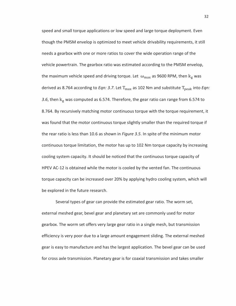
vehicle powertrain. The gearbox ratio was estimated according to the PMSM envelop,
the maximum vehicle speed and driving torque. Let as 9600 RPM, then was
derived as 8.764 according to Eqn: 3.7. Let as 102 Nm and substitute into Eqn:
3.6, then was computed as 6.574. Therefore, the gear ratio can range from 6.574 to
8.764. By recursively matching motor continuous torque with the torque requirement, it
was found that the motor continuous torque slightly smaller than the required torque if
the rear ratio is less than 10.6 as shown in Figure 3.5. In spite of the minimum motor
continuous torque limitation, the motor has up to 102 Nm torque capacity by increasing
cooling system capacity. It should be noticed that the continuous torque capacity of
HPEV AC-12 is obtained while the motor is cooled by the vented fan. The continuous
torque capacity can be increased over 20% by applying hydro cooling system, which will
be explored in the future research.
Several types of gear can provide the estimated gear ratio. The worm set,
external meshed gear, bevel gear and planetary set are commonly used for motor
gearbox. The worm set offers very large gear ratio in a single mesh, but transmission
efficiency is very poor due to a large amount engagement sliding. The external meshed
gear is easy to manufacture and has the largest application. The bevel gear can be used
for cross axle transmission. Planetary gear is for coaxial transmission and takes smaller
33
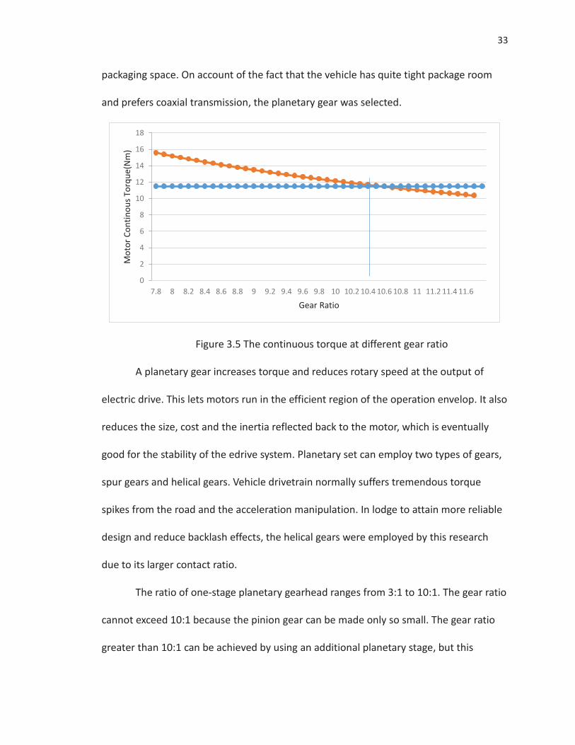
packaging space. On account of the fact that the vehicle has quite tight package room
and prefers coaxial transmission, the planetary gear was selected.
Figure 3.5 The continuous torque at different gear ratio
A planetary gear increases torque and reduces rotary speed at the output of
electric drive. This lets motors run in the efficient region of the operation envelop. It also
reduces the size, cost and the inertia reflected back to the motor, which is eventually
good for the stability of the edrive system. Planetary set can employ two types of gears,
spur gears and helical gears. Vehicle drivetrain normally suffers tremendous torque
spikes from the road and the acceleration manipulation. In lodge to attain more reliable
design and reduce backlash effects, the helical gears were employed by this research
due to its larger contact ratio.
The ratio of one-stage planetary gearhead ranges from 3:1 to 10:1. The gear ratio
cannot exceed 10:1 because the pinion gear can be made only so small. The gear ratio
greater than 10:1 can be achieved by using an additional planetary stage, but this
0
2
4
6
8
10
12
14
16
18
7.8 8 8.2 8.4 8.6 8.8 9 9.2 9.4 9.6 9.8 10 10.2 10.4 10.6 10.8 11 11.2 11.4 11.6
Mot
or C
ontin
ous
Torq
ue(N
m)
Gear Ratio
34
normally increases the length and price of the gearhead. Based on the research
conducted by Horn and Dale (2012), ratios between 4:1 and 8:1 provide the best
combination of pinion and planet-gear size, performance, and life. Hence, this research
selected a helical planetary gear set with the reduction ratio, 8.0. Consequentially, this
research increased the cooling system capacity 30% to fill the continuous torque gap of
the HPEV AC-12. On the basis of the motor operation envelop, the battery system was
sized.
3.1.3.3 Battery
This research disscussed the battery types and sizing for the IAWDEV application.
The EV powertrain generally requires high power, extended cycle life and great safety.
Karden, Ploumen and Fricke (2007) presented that NiMH and Li-ion are dominating the
current and potential battery technologies for EVs and HEV. Sinkaram et al. (2012)
concluded that lithium-ion battery has better energy densities, higher power density and
longer cycling life comparing the lead-acid battery and nickel metal hydride battery. With
some changes to the battery comparison in Sinkaram et al. (2012) and the test curve of
batter cycle life in the A123 white paper, the comparison chart was obtained as shown in
Figure 3.6. Figure 3.6 shows that the NiMH has larger discharge rate and longer cycle life
than the Lead-acid and the traditional Li-ion; NiMH seems the best option in a decade
ago. However, Karden, Ploumen and Fricke (2007) found that the high-performance
lithium-ion batteries have achieved better performance and brought down their cost to
the range of NiMH. For instance, A123 System, LLC. patented the high performance

35
Nanophosphate Li-ion battery that can extend the cycle life up to 7,000 and provide up
to 35C discharge rate.
According to the plausible performance of high-performance Li-ion batteries and
its continuous improvements in performance and cost, this research selected the high-
performance Li-ion battery as the high voltage electric storage system. The battery
modules and parameters were calculated based on the 6x15s2p battery pack provided
by A123 Systems, LLC; the parameters were listed in Table 3.6.
Figure 3.6 The battery comparison
Table 3.6 provides both continuous and peak operation parameters. The peak
operation has 10 seconds duration. These parameters and electric drive power
requirements were employed to calculate battery pack architecture and amount of
90
62.5
40
125
5
20
5
35
4
15
3
70
-10
10
30
50
70
90
110
130
Lead-acid NiMH Li-ion Li-ion Nanophosphate(A123)
Battery Types Comparison
Energy Density (Wh/kg) Peak Discharge Rate ( C ) Cycle Life (X100 Cycles)
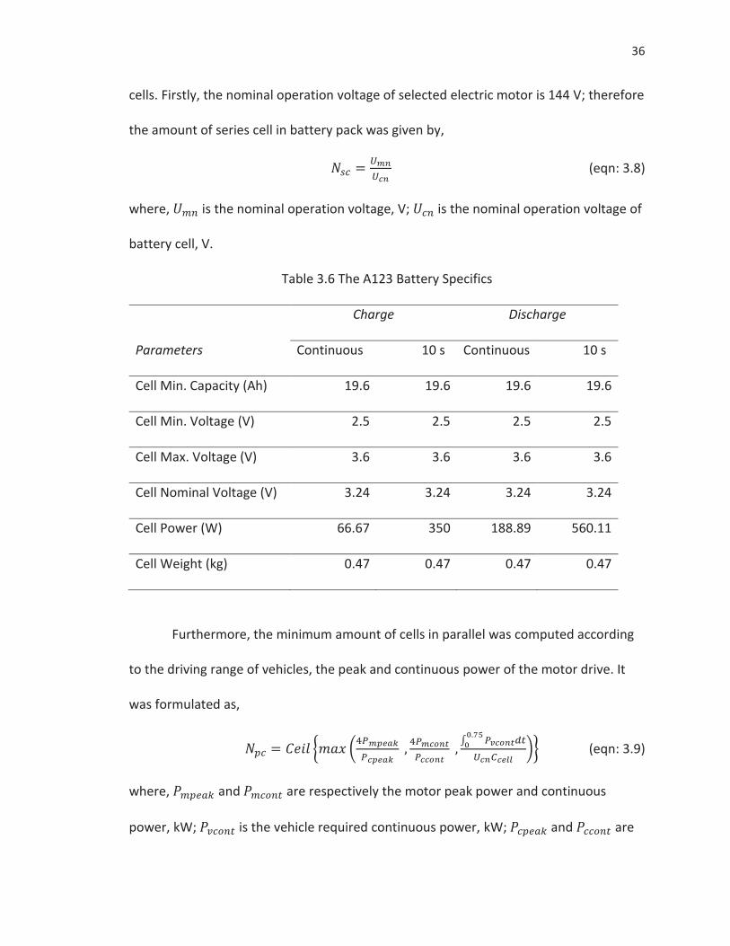
36
cells. Firstly, the nominal operation voltage of selected electric motor is 144 V; therefore
the amount of series cell in battery pack was given by,
(eqn: 3.8)
where, is the nominal operation voltage, V; is the nominal operation voltage of
battery cell, V.
Table 3.6 The A123 Battery Specifics
Parameters
Charge Discharge
Continuous 10 s Continuous 10 s
Cell Min. Capacity (Ah) 19.6 19.6 19.6 19.6
Cell Min. Voltage (V) 2.5 2.5 2.5 2.5
Cell Max. Voltage (V) 3.6 3.6 3.6 3.6
Cell Nominal Voltage (V) 3.24 3.24 3.24 3.24
Cell Power (W) 66.67 350 188.89 560.11
Cell Weight (kg) 0.47 0.47 0.47 0.47
Furthermore, the minimum amount of cells in parallel was computed according
to the driving range of vehicles, the peak and continuous power of the motor drive. It
was formulated as,
(eqn: 3.9)
where, and are respectively the motor peak power and continuous
power, kW; is the vehicle required continuous power, kW; and are
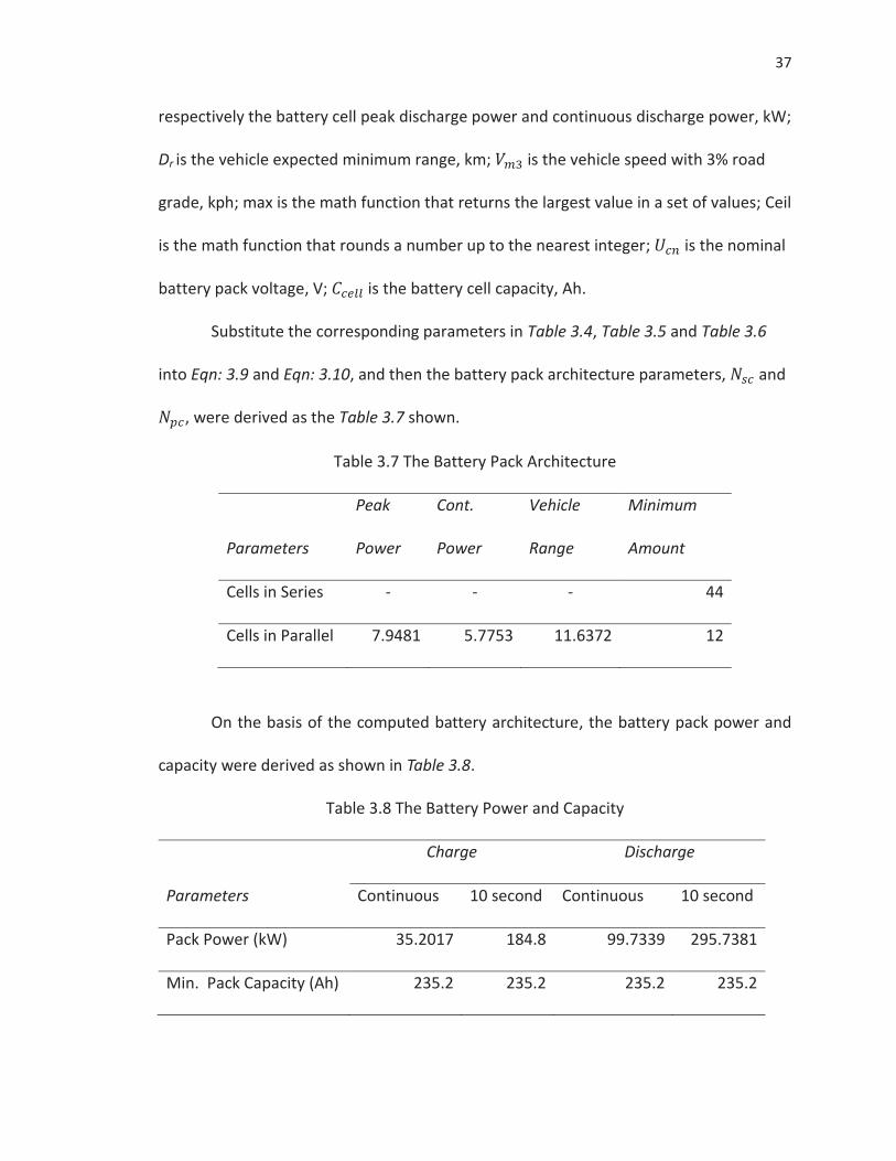
37
respectively the battery cell peak discharge power and continuous discharge power, kW;
Dr is the vehicle expected minimum range, km; is the vehicle speed with 3% road
grade, kph; max is the math function that returns the largest value in a set of values; Ceil
is the math function that rounds a number up to the nearest integer; is the nominal
battery pack voltage, V; is the battery cell capacity, Ah.
Substitute the corresponding parameters in Table 3.4, Table 3.5 and Table 3.6
into Eqn: 3.9 and Eqn: 3.10, and then the battery pack architecture parameters, and
, were derived as the Table 3.7 shown.
Table 3.7 The Battery Pack Architecture
Parameters
Peak
Power
Cont.
Power
Vehicle
Range
Minimum
Amount
Cells in Series - - - 44
Cells in Parallel 7.9481 5.7753 11.6372 12
On the basis of the computed battery architecture, the battery pack power and
capacity were derived as shown in Table 3.8.
Table 3.8 The Battery Power and Capacity
Parameters
Charge Discharge
Continuous 10 second Continuous 10 second
Pack Power (kW) 35.2017 184.8 99.7339 295.7381
Min. Pack Capacity (Ah) 235.2 235.2 235.2 235.2
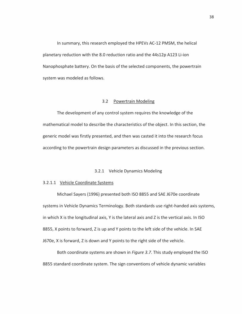
38
In summary, this research employed the HPEVs AC-12 PMSM, the helical
planetary reduction with the 8.0 reduction ratio and the 44s12p A123 Li-ion
Nanophosphate battery. On the basis of the selected components, the powertrain
system was modeled as follows.
3.2 Powertrain Modeling
The development of any control system requires the knowledge of the
mathematical model to describe the characteristics of the object. In this section, the
generic model was firstly presented, and then was casted it into the research focus
according to the powertrain design parameters as discussed in the previous section.
3.2.1 Vehicle Dynamics Modeling
3.2.1.1 Vehicle Coordinate Systems
Michael Sayers (1996) presented both ISO 8855 and SAE J670e coordinate
systems in Vehicle Dynamics Terminology. Both standards use right-handed axis systems,
in which X is the longitudinal axis, Y is the lateral axis and Z is the vertical axis. In ISO
8855, X points to forward, Z is up and Y points to the left side of the vehicle. In SAE
J670e, X is forward, Z is down and Y points to the right side of the vehicle.
Both coordinate systems are shown in Figure 3.7. This study employed the ISO
8855 standard coordinate system. The sign conventions of vehicle dynamic variables
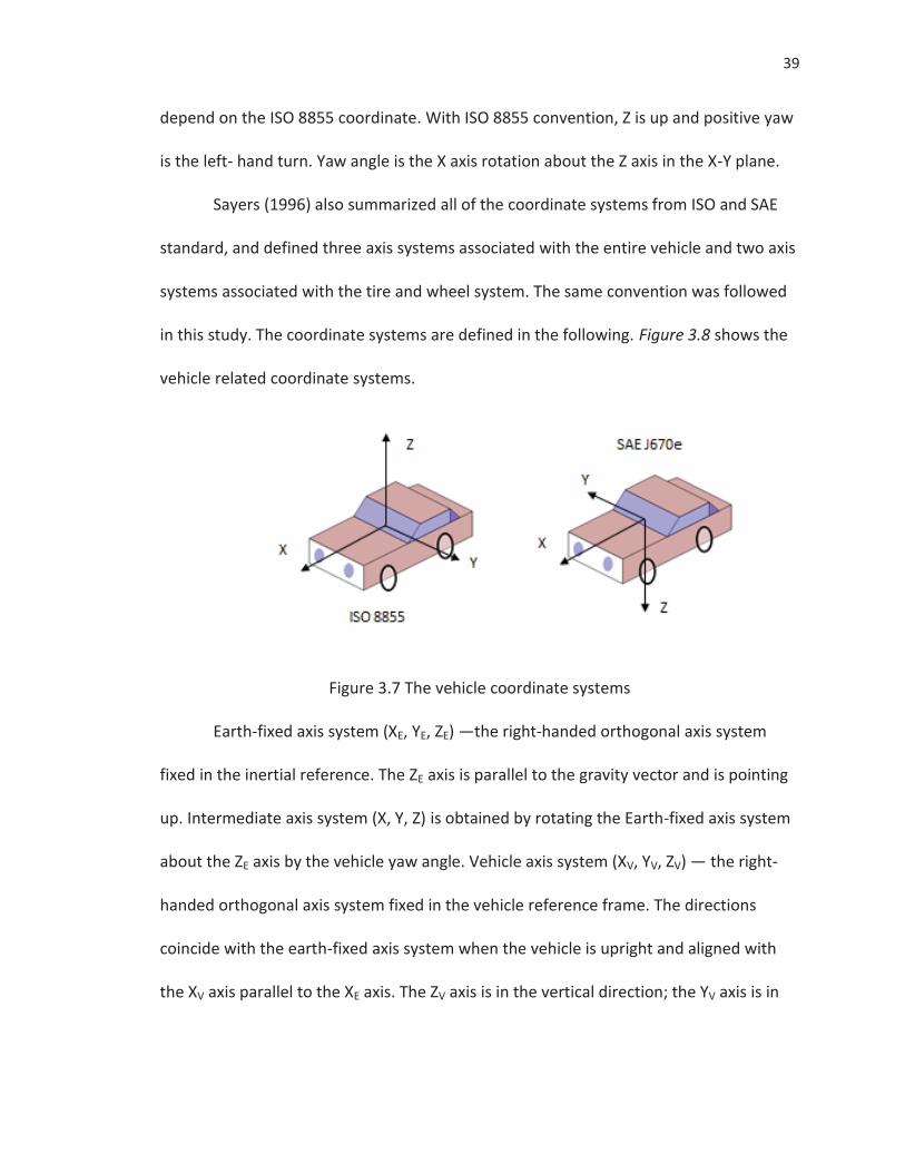
39
depend on the ISO 8855 coordinate. With ISO 8855 convention, Z is up and positive yaw
is the left- hand turn. Yaw angle is the X axis rotation about the Z axis in the X-Y plane.
Sayers (1996) also summarized all of the coordinate systems from ISO and SAE
standard, and defined three axis systems associated with the entire vehicle and two axis
systems associated with the tire and wheel system. The same convention was followed
in this study. The coordinate systems are defined in the following. Figure 3.8 shows the
vehicle related coordinate systems.
Figure 3.7 The vehicle coordinate systems
Earth-fixed axis system (XE, YE, ZE) —the right-handed orthogonal axis system
fixed in the inertial reference. The ZE axis is parallel to the gravity vector and is pointing
up. Intermediate axis system (X, Y, Z) is obtained by rotating the Earth-fixed axis system
about the ZE axis by the vehicle yaw angle. Vehicle axis system (XV, YV, ZV) — the right-
handed orthogonal axis system fixed in the vehicle reference frame. The directions
coincide with the earth-fixed axis system when the vehicle is upright and aligned with
the XV axis parallel to the XE axis. The ZV axis is in the vertical direction; the YV axis is in
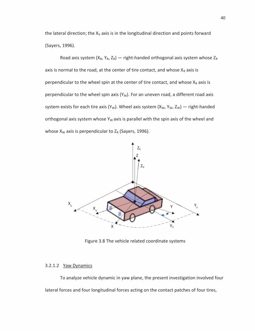
40
the lateral direction; the XV axis is in the longitudinal direction and points forward
(Sayers, 1996).
Road axis system (XR, YR, ZR) — right-handed orthogonal axis system whose ZR
axis is normal to the road, at the center of tire contact, and whose XR axis is
perpendicular to the wheel spin at the center of tire contact, and whose XR axis is
perpendicular to the wheel spin axis (YW). For an uneven road, a different road axis
system exists for each tire axis (YW). Wheel axis system (XW, YW, ZW) — right-handed
orthogonal axis system whose YW axis is parallel with the spin axis of the wheel and
whose XW axis is perpendicular to ZR (Sayers, 1996).
Figure 3.8 The vehicle related coordinate systems
3.2.1.2 Yaw Dynamics
To analyze vehicle dynamic in yaw plane, the present investigation involved four
lateral forces and four longitudinal forces acting on the contact patches of four tires,
ZE
XE Y
E
XV
X YV
ZV
Z
Y
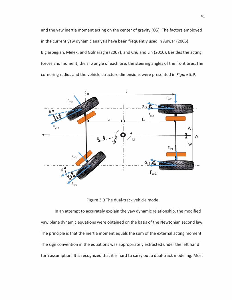
41
and the yaw inertia moment acting on the center of gravity (CG). The factors employed
in the current yaw dynamic analysis have been frequently used in Anwar (2005),
Biglarbegian, Melek, and Golnaraghi (2007), and Chu and Lin (2010). Besides the acting
forces and moment, the slip angle of each tire, the steering angles of the front tires, the
cornering radius and the vehicle structure dimensions were presented in Figure 3.9.
Figure 3.9 The dual-track vehicle model
In an attempt to accurately explain the yaw dynamic relationship, the modified
yaw plane dynamic equations were obtained on the basis of the Newtonian second law.
The principle is that the inertia moment equals the sum of the external acting moment.
The sign convention in the equations was appropriately extracted under the left hand
turn assumption. It is recognized that it is hard to carry out a dual-track modeling. Most
W W
W2
W
Lr Lf
Fxf1
Fxf2
Fxr2
Fxr1
M
Fyf2
Fyf1
Fyr1
Fyr2
β
L
δ1
δ2
αf1
αf2
αr2
αr1
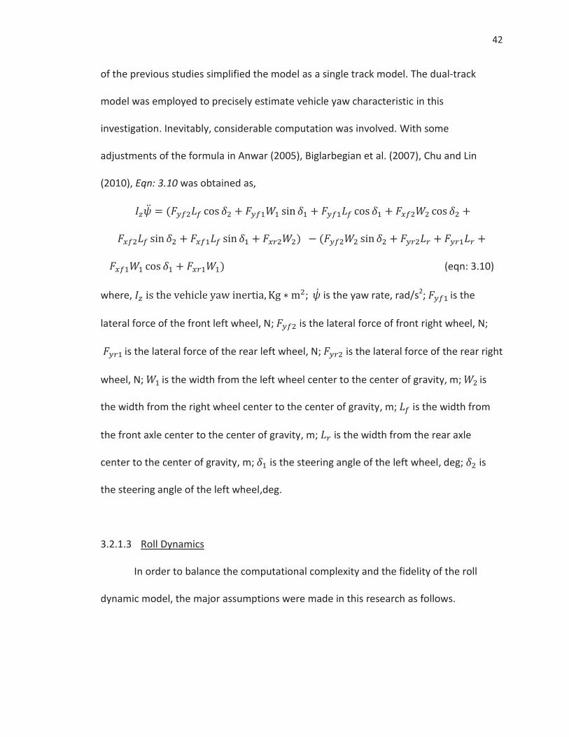
42
of the previous studies simplified the model as a single track model. The dual-track
model was employed to precisely estimate vehicle yaw characteristic in this
investigation. Inevitably, considerable computation was involved. With some
adjustments of the formula in Anwar (2005), Biglarbegian et al. (2007), Chu and Lin
(2010), Eqn: 3.10 was obtained as,
(eqn: 3.10)
where, is the yaw rate, rad/s2; is the
lateral force of the front left wheel, N; is the lateral force of front right wheel, N;
is the lateral force of the rear left wheel, N; is the lateral force of the rear right
wheel, N; is the width from the left wheel center to the center of gravity, m; is
the width from the right wheel center to the center of gravity, m; is the width from
the front axle center to the center of gravity, m; is the width from the rear axle
center to the center of gravity, m; is the steering angle of the left wheel, deg; is
the steering angle of the left wheel,deg.
3.2.1.3 Roll Dynamics
In order to balance the computational complexity and the fidelity of the roll
dynamic model, the major assumptions were made in this research as follows.
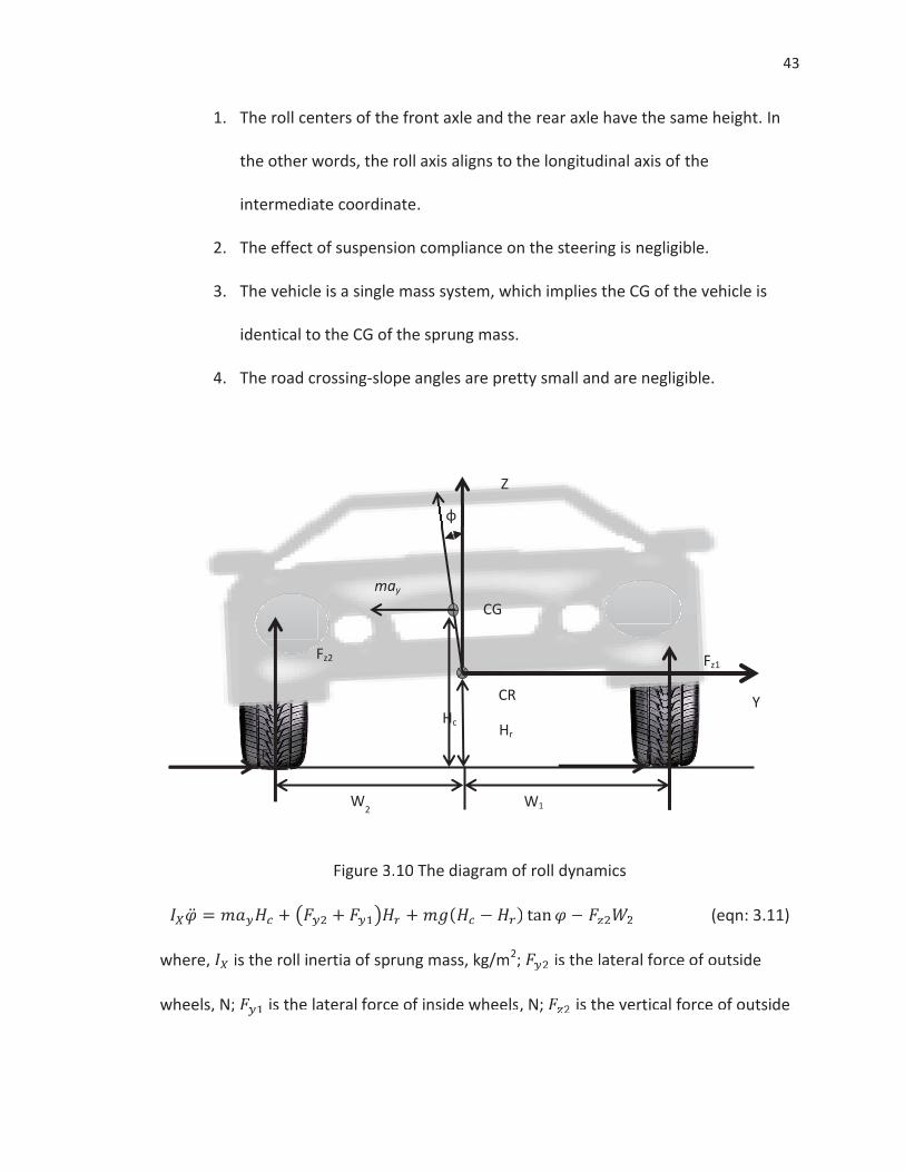
43
1. The roll centers of the front axle and the rear axle have the same height. In
the other words, the roll axis aligns to the longitudinal axis of the
intermediate coordinate.
2. The effect of suspension compliance on the steering is negligible.
3. The vehicle is a single mass system, which implies the CG of the vehicle is
identical to the CG of the sprung mass.
4. The road crossing-slope angles are pretty small and are negligible.
Figure 3.10 The diagram of roll dynamics
(eqn: 3.11)
where, is the roll inertia of sprung mass, kg/m2; is the lateral force of outside
wheels, N; is the lateral force of inside wheels, N; is the vertical force of outside
Figure 3.10 The diagram of roll dynamics
(eqn
re, is the roll inertia of sprung mass, kg/m2; is the lateral force of outsi
els, N; is the lateral force of inside wheels, N; is the vertical force of o
φ
W2 W1
CG
CR
Fy2
Hr
Y
Fz1 Fz2
Z
Hc
Fy1
may
44
wheels, N; is the height of roll center, m; is the height of CG, m; and the
relationship between and was defined as,
(eqn: 3.12)
where, Cr is the ratio of the roll center and CG height. In this study, it is 0.5.
3.2.1.4 Weight Transfer
The forces acting on inside wheels and outside wheels are strongly related to
lateral load transfer. In a steady state cornering, the relationship was developed by
taking moments about outside of the tire patch center,
(eqn: 3.13)
It is readily proved that the steering angle and the tire slip angle fulfill the
causality. In further, the roll angle, , is the one time step lag response of the lateral
acceleration, . The current step lateral acceleration is derived according to the
previous step roll angle. In order to further simplify equations, the backshift operator
was introduced in this research. The back shift operator is defined by Robert and David
(2010) as,
(eqn: 3.14)
and it also extends to powers,
(eqn: 3.15)
and
(eqn: 3.16)
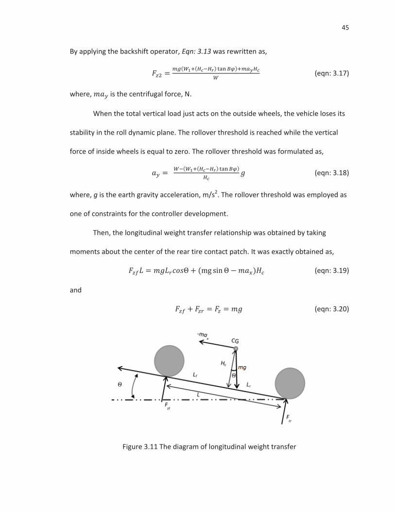
45
By applying the backshift operator, Eqn: 3.13 was rewritten as,
(eqn: 3.17)
where, is the centrifugal force, N.
When the total vertical load just acts on the outside wheels, the vehicle loses its
stability in the roll dynamic plane. The rollover threshold is reached while the vertical
force of inside wheels is equal to zero. The rollover threshold was formulated as,
(eqn: 3.18)
where, g is the earth gravity acceleration, m/s2. The rollover threshold was employed as
one of constraints for the controller development.
Then, the longitudinal weight transfer relationship was obtained by taking
moments about the center of the rear tire contact patch. It was exactly obtained as,
(eqn: 3.19)
and
(eqn: 3.20)
Figure 3.11 The diagram of longitudinal weight transfer
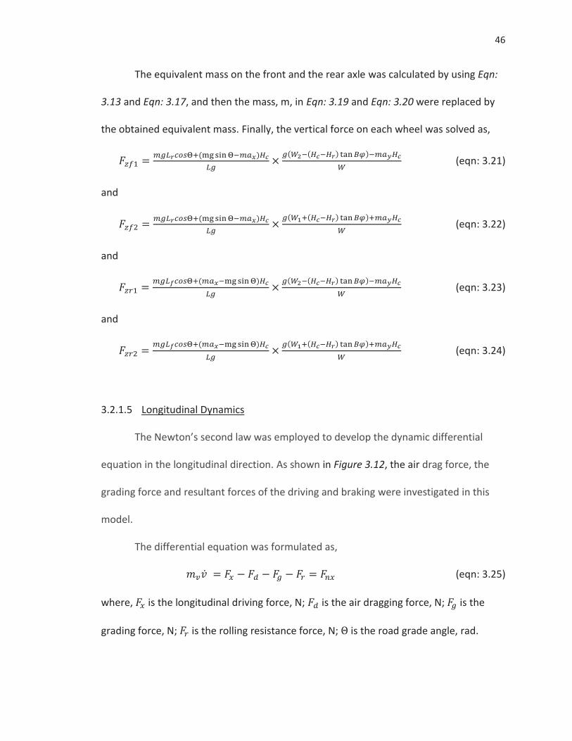
46
The equivalent mass on the front and the rear axle was calculated by using Eqn:
3.13 and Eqn: 3.17, and then the mass, m, in Eqn: 3.19 and Eqn: 3.20 were replaced by
the obtained equivalent mass. Finally, the vertical force on each wheel was solved as,
(eqn: 3.21)
and
(eqn: 3.22)
and
(eqn: 3.23)
and
(eqn: 3.24)
3.2.1.5 Longitudinal Dynamics
The Newton’s second law was employed to develop the dynamic differential
equation in the longitudinal direction. As shown in Figure 3.12, the air drag force, the
grading force and resultant forces of the driving and braking were investigated in this
model.
The differential equation was formulated as,
(eqn: 3.25)
where, is the longitudinal driving force, N; is the air dragging force, N; is the
grading force, N; is the rolling resistance force, N; is the road grade angle, rad.
47
Figure 3.12 The diagram of longitudinal dynamics
Sequentially, the longitudinal resultant forces were further derived as.
(eqn: 3.26)
and
(eqn: 3.27)
and
(eqn: 3.28)
and
(eqn: 3.29)
and
(eqn: 3.30)
and
mg
48
(eqn: 3.31)
where, is the torque produced by the front left wheel, Nm; is the torque
produced by the front right wheel, Nm; is the torque produced by the front left
wheel, Nm; is the torque produced by the front right wheel, Nm; is the dynamic
radius of tires, m; Af is the vehicle front area, m2; Cd is the aerodynamic drag coefficient,
; is the air density, 1.25 Kg/m3; is the rolling resistance coefficient.
The above equations illustrate that the load briefly consists of rolling resistance,
road gradient, acceleration and air drag; the traction force is provided by the electric
motors. The traction force acting on the vehicle is also limited by the ground grip ability.
The effective longitudinal force was calculated by,
(eqn: 3.32)
where, is the longitudinal driving forces; , ; is the ground
grip forces, , ; the ground grip force is calculated by,
(eqn: 3.33)
where, g is the gravity acceleration, m/s2; is the grip coefficient.
3.2.1.6 Vehicle Slip Angle
The generalized vehicle slip angle was formulated in analogy to the tire slip angle.
The vehicle slip angle is defined as the angle between its velocity vector at CG and
longitudinal axis of the vehicle. It was practically calculated by,
(eqn: 3.34)
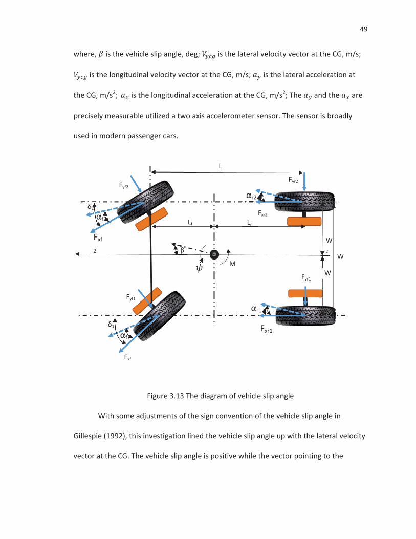
49
where, is the vehicle slip angle, deg; is the lateral velocity vector at the CG, m/s;
is the longitudinal velocity vector at the CG, m/s; is the lateral acceleration at
the CG, m/s2; is the longitudinal acceleration at the CG, m/s2; The and the are
precisely measurable utilized a two axis accelerometer sensor. The sensor is broadly
used in modern passenger cars.
Figure 3.13 The diagram of vehicle slip angle
With some adjustments of the sign convention of the vehicle slip angle in
Gillespie (1992), this investigation lined the vehicle slip angle up with the lateral velocity
vector at the CG. The vehicle slip angle is positive while the vector pointing to the
W2
W
Lr Lf
Fxf
Fxf
2
Fxr2
Fxr1
M
Fyf2
Fyf1
Fyr1
Fyr2
β
L
W
δ1
δ2
αf1
αf2
αr2
αr1
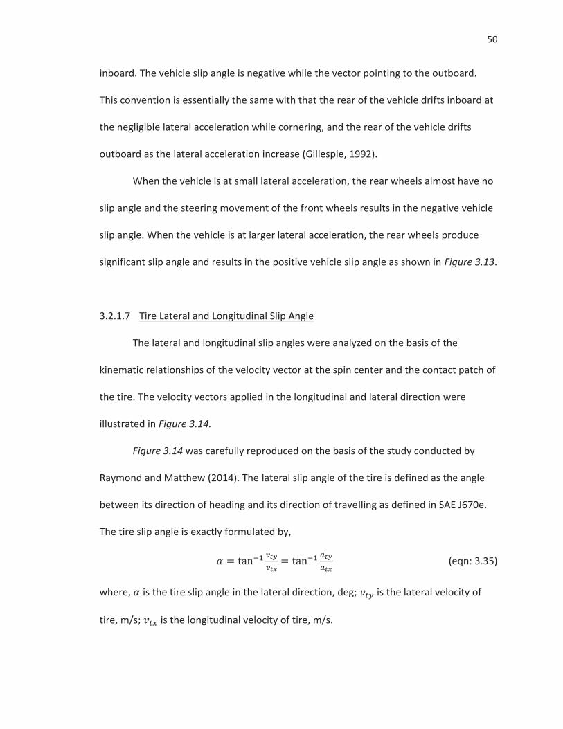
50
inboard. The vehicle slip angle is negative while the vector pointing to the outboard.
This convention is essentially the same with that the rear of the vehicle drifts inboard at
the negligible lateral acceleration while cornering, and the rear of the vehicle drifts
outboard as the lateral acceleration increase (Gillespie, 1992).
When the vehicle is at small lateral acceleration, the rear wheels almost have no
slip angle and the steering movement of the front wheels results in the negative vehicle
slip angle. When the vehicle is at larger lateral acceleration, the rear wheels produce
significant slip angle and results in the positive vehicle slip angle as shown in Figure 3.13.
3.2.1.7 Tire Lateral and Longitudinal Slip Angle
The lateral and longitudinal slip angles were analyzed on the basis of the
kinematic relationships of the velocity vector at the spin center and the contact patch of
the tire. The velocity vectors applied in the longitudinal and lateral direction were
illustrated in Figure 3.14.
Figure 3.14 was carefully reproduced on the basis of the study conducted by
Raymond and Matthew (2014). The lateral slip angle of the tire is defined as the angle
between its direction of heading and its direction of travelling as defined in SAE J670e.
The tire slip angle is exactly formulated by,
(eqn: 3.35)
where, is the tire slip angle in the lateral direction, deg; is the lateral velocity of
tire, m/s; is the longitudinal velocity of tire, m/s.
51
Figure 3.14 The lateral tire slip angle
It should be noticed that the lateral velocity and acceleration of tires are quite
difficult to be measured in practice. The observer was thus designed in this research to
estimate the lateral slip angle of the tire. The observer is based on the generic rules of
strain and stress; in other words, the lateral tire slip angle is the ratio between the
lateral stress and the cornering stiffness which is formulated as,
(eqn: 3.36)
where, i is the index of tires; is the vehicle turning radius, m; is the tire cornering
stiffness, N/deg; is the distribution factor of the lateral force.
The longitudinal slip has various definitions. The present research employed that
the longitudinal tire slip is the ratio of the linear velocity at tire outer surface and the
velocity at the spin center of the tire. This definition is commonly used in the previous
researches. It is accurately calculated by,
(eqn: 3.37)
vty
vtx α
52
where, is the tire dynamic diameter, m; is the tire rotary speed, RPS.
3.2.1.8 Tire and Vehicle Slip Angle Relationship
As presented in the previous section, the tire slip angle can be theoretically
calculated. In fact, the tire lateral slip angle is hard to be measured practically. In order
to avoid this limitation, the kinematic relationship between tire and vehicle slip angle
relationship was developed. The relationship was adjusted according to Bosch
Automotive Handbook (2004). It is given by,
(eqn: 3.38)
and
(eqn: 3.39)
and
(eqn: 3.40)
and
(eqn: 3.41)
where, is the front left tire slip angle, deg; is the front right tire slip angle,
deg; is the rear left tire slip angle, deg; is the rear right tire slip angle, deg;
The lateral forces produced by the tires lateral slip, , , and ,
were obtained by using the non-linear Dugoff’s tire model in Bian et al. (2014) and Smith
and Starkey (1995). The model is formulated as,
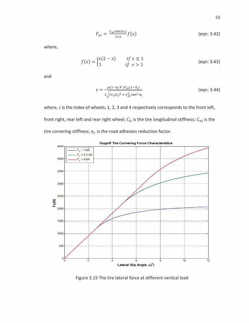
53
(eqn: 3.42)
where,
(eqn: 3.43)
and
(eqn: 3.44)
where, is the index of wheels; 1, 2, 3 and 4 respectively corresponds to the front left,
front right, rear left and rear right wheel; is the tire longitudinal stiffness; is the
tire cornering stiffness; is the road adhesion reduction factor.
Figure 3.15 The tire lateral force at different vertical load
54
The non-linear Dugoff’s tire model was employed to the P225/55 R18 tires in this
research. The tire data are shown in Appendix E. Eqn: 3.44 shows that the vertical load
on the tire implicitly impacts on the lateral force. In order to visualize the effect of the
vertical load, Eqn: 3.42, 3.43 and 3.44 were modeled in Simulink. The simulation results
are presented in Figure 3.15.
3.2.1.9 Steering Angles
During cornering, the steering angle of the inside wheel is larger than the
steering angle of the inside wheel. In 1759, Darwin specified the principle that should
ideally be followed that the two front wheels should turn about the center that lies on
the extended line of the back axle of the carriage (King-Hele, 2002). The Darwin’s
principle was shown in Figure 3.16; Figure 3.16 was reproduced on the basis of the
diagram in King-Hele (2002).
In principle, the steering angles of the wheels were estimated according to
Darwin and Lankensperger steering geometry, as shown in Figure 3.16. For large
steering angles, the vehicle turning center moves forward slightly, but it is almost as
good as being on the line of the back axle (King-Hele, 2002).
The steering angle of the both front wheels was considered in the small lateral
acceleration condition and also the large lateral acceleration. The ranges of lateral
acceleration are essentially identical to the definition in Bosch Automotive Handbook
(2004). The small lateral acceleration ranges from 0 m/s to 0.5 m/s. The large lateral
acceleration ranges from 0.5m/s to 4m/s.
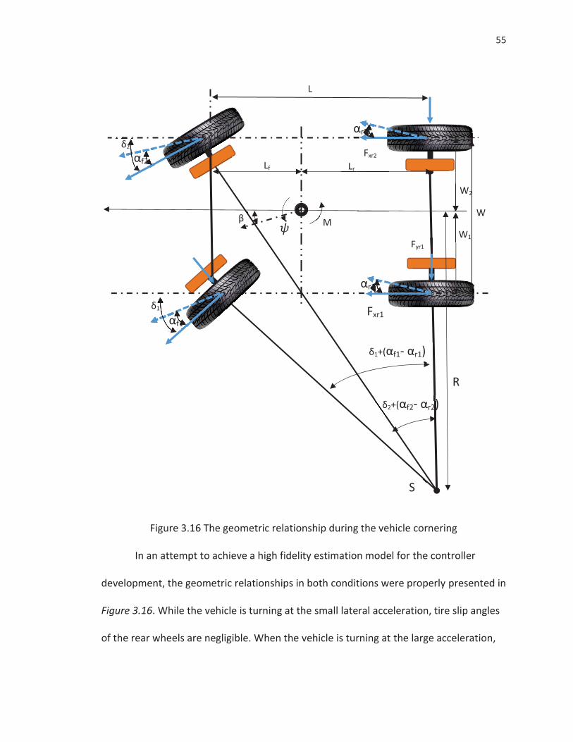
55
Figure 3.16 The geometric relationship during the vehicle cornering
In an attempt to achieve a high fidelity estimation model for the controller
development, the geometric relationships in both conditions were properly presented in
Figure 3.16. While the vehicle is turning at the small lateral acceleration, tire slip angles
of the rear wheels are negligible. When the vehicle is turning at the large acceleration,
W W
W2
W1
Lr Lf
Fxr2
Fxr1
M
Fyr1
β
L
R
S
δ1
δ1+(αf1- αr1)
δ2+(αf2- αr2)
δ2
αf1
αf2
αr2
αr1
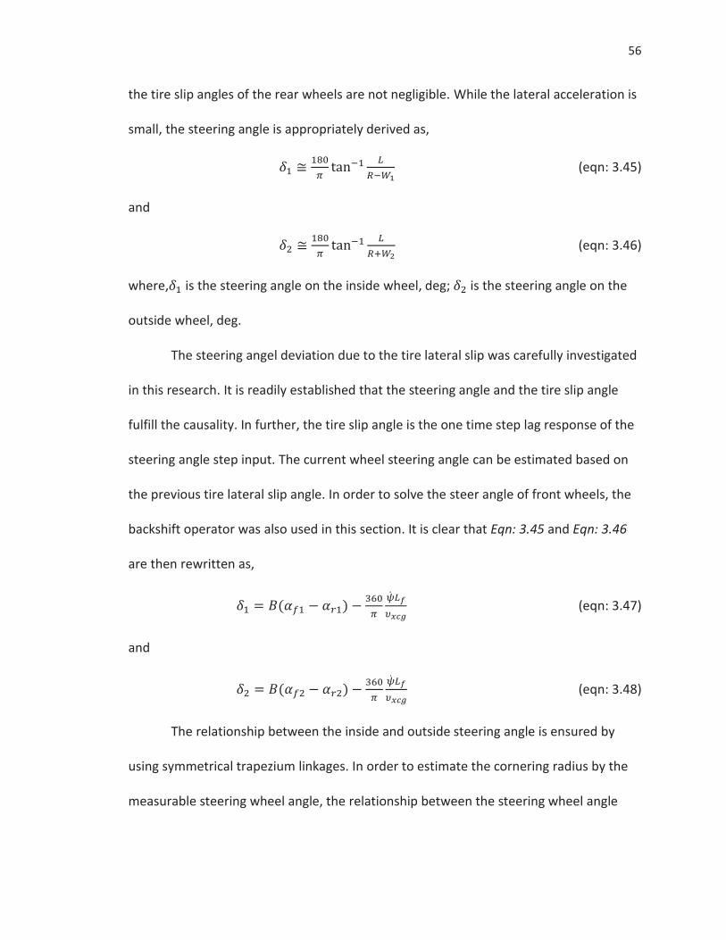
56
the tire slip angles of the rear wheels are not negligible. While the lateral acceleration is
small, the steering angle is appropriately derived as,
(eqn: 3.45)
and
(eqn: 3.46)
where, is the steering angle on the inside wheel, deg; is the steering angle on the
outside wheel, deg.
The steering angel deviation due to the tire lateral slip was carefully investigated
in this research. It is readily established that the steering angle and the tire slip angle
fulfill the causality. In further, the tire slip angle is the one time step lag response of the
steering angle step input. The current wheel steering angle can be estimated based on
the previous tire lateral slip angle. In order to solve the steer angle of front wheels, the
backshift operator was also used in this section. It is clear that Eqn: 3.45 and Eqn: 3.46
are then rewritten as,
(eqn: 3.47)
and
(eqn: 3.48)
The relationship between the inside and outside steering angle is ensured by
using symmetrical trapezium linkages. In order to estimate the cornering radius by the
measurable steering wheel angle, the relationship between the steering wheel angle
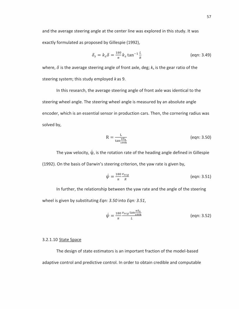
57
and the average steering angle at the center line was explored in this study. It was
exactly formulated as proposed by Gillespie (1992),
(eqn: 3.49)
where, is the average steering angle of front axle, deg; ks is the gear ratio of the
steering system; this study employed k as 9.
In this research, the average steering angle of front axle was identical to the
steering wheel angle. The steering wheel angle is measured by an absolute angle
encoder, which is an essential sensor in production cars. Then, the cornering radius was
solved by,
(eqn: 3.50)
The yaw velocity, , is the rotation rate of the heading angle defined in Gillespie
(1992). On the basis of Darwin’s steering criterion, the yaw rate is given by,
(eqn: 3.51)
In further, the relationship between the yaw rate and the angle of the steering
wheel is given by substituting Eqn: 3.50 into Eqn: 3.51,
(eqn: 3.52)
3.2.1.10 State Space
The design of state estimators is an important fraction of the model-based
adaptive control and predictive control. In order to obtain credible and computable
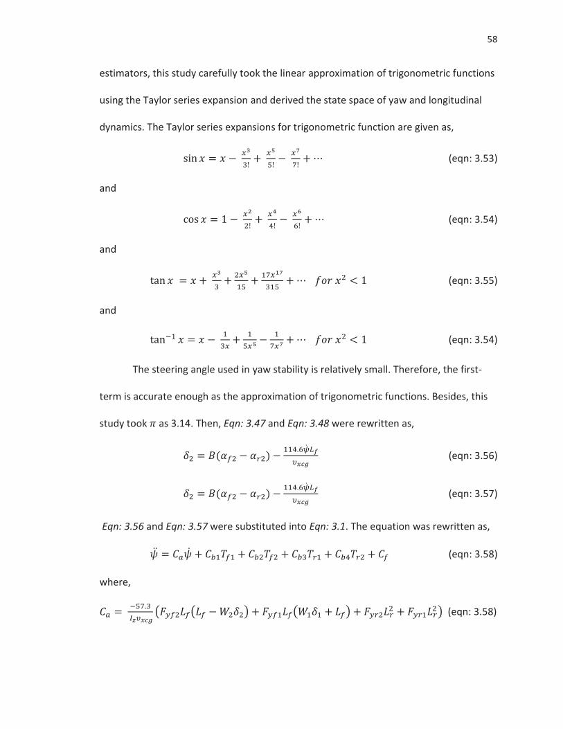
58
estimators, this study carefully took the linear approximation of trigonometric functions
using the Taylor series expansion and derived the state space of yaw and longitudinal
dynamics. The Taylor series expansions for trigonometric function are given as,
(eqn: 3.53)
and
(eqn: 3.54)
and
(eqn: 3.55)
and
(eqn: 3.54)
The steering angle used in yaw stability is relatively small. Therefore, the first-
term is accurate enough as the approximation of trigonometric functions. Besides, this
study took as 3.14. Then, Eqn: 3.47 and Eqn: 3.48 were rewritten as,
(eqn: 3.56)
(eqn: 3.57)
Eqn: 3.56 and Eqn: 3.57 were substituted into Eqn: 3.1. The equation was rewritten as,
(eqn: 3.58)
where,
(eqn: 3.58)
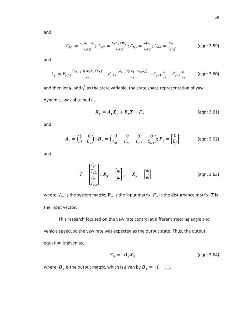
59
and
; ; ; ; (eqn: 3.59)
and
(eqn: 3.60)
and then let and as the state variable, the state space representation of yaw
dynamics was obtained as,
(eqn: 3.61)
and
; ; ; (eqn: 3.62)
and
(eqn: 3.63)
where, is the system matrix; is the input matrix; is the disturbance matrix; is
the input vector.
This research focused on the yaw rate control at different steering angle and
vehicle speed, so the yaw rate was expected as the output state. Thus, the output
equation is given as,
(eqn: 3.64)
where, is the output matrix, which is given by .
60
Furthermore, was as a state variable. The state space equation of
longitudinal dynamics was obtained as,
(eqn: 3.65)
where,
; (eqn: 3.66)
and
(eqn: 3.67)
3.2.2 Electric Drive System
The motor drive and the battery system are two primary components of the
IAWDEV. The motor drive modeling includes the mathematical transformation and the
equivalent DC motor model. The battery system modeling covers the terminal voltage,
thermal effects and state of charge. Most models of the electric drive assembly were
obtained according to the Kirchhoff’s laws, Ohm’s law, Faraday’s law and the definitions
of electric circuit components, such as resistance, inductance and capacitance. These
laws and definitions are the fundamental tools for electric system modeling for various
researches.
61
3.2.2.1 Motor Drive
3.2.2.1.1 Mathematical Transformation
A great deal of the three-phase PMSM modeling and control involves
transforming observed vectors from one coordinate system to another. Therefore, it is
convenient to discuss the generic conventions of the coordinate transformation in the
first place. These appropriate rules would be applied to specific problems in the motor
modeling and control.
There are numerous mathematical methods to undertake the coordinate
transformation, whereas this study focused itself on linear transformations. These
transformations map the coordinates in one reference frame to those in another by
methods of a set of linear algebraic equations. In vector notation, it is written as,
(eqn: 3.68)
where, is the components vector of the coordinate system in the first frame; is the
component vector of the coordinate system in the second frame; is the origin offset
vector from the first coordinate system to the second coordinate system; A is the
transformation matrix.
In order to describe a vector in a convenient manner, its length shouldn’t depend
on the coordinate system. Hence, the linear transformation should be restricted to
special sets of linear transformations. In other words, the transformation matrix must
satisfy the following condition,
(eqn: 3.69)
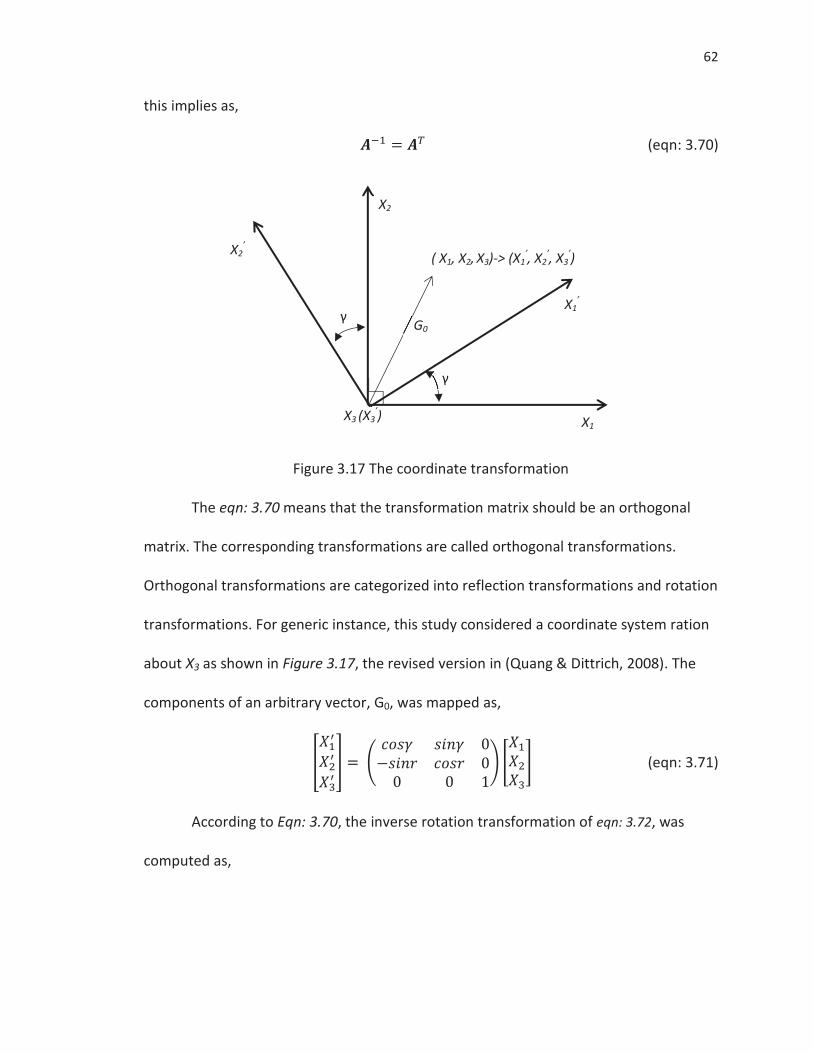
62
this implies as,
(eqn: 3.70)
Figure 3.17 The coordinate transformation
The eqn: 3.70 means that the transformation matrix should be an orthogonal
matrix. The corresponding transformations are called orthogonal transformations.
Orthogonal transformations are categorized into reflection transformations and rotation
transformations. For generic instance, this study considered a coordinate system ration
about X3 as shown in Figure 3.17, the revised version in (Quang & Dittrich, 2008). The
components of an arbitrary vector, G0, was mapped as,
(eqn: 3.71)
According to Eqn: 3.70, the inverse rotation transformation of eqn: 3.72, was
computed as,
X1
γ
X2
X2’
X1’
γ
( X1, X2, X3)-> (X1’, X2
’, X3’)
X3 (X3’)
G0
63
(eqn: 3.73)
3.2.2.1.2 Motor Modeling
In order to support more complex control of the PMSM, this study developed the
motor model in analogy to the separately excited DC motor. However, the alternating
current synchronous machines do not have the same key features as the DC motor
(Bhardwaj, 2013). In the PMSM, the field excitation is produced by the permanent
magnetic equally spaced on the rotor; only one source, the stator current, can be
controlled. For the sake of the modeling simplification as the excited DC motor, the
three-phase components were orthogonally decomposed as the torque and the
magnetizing flux component of the stator current. The decomposed components were
respectively appointed as the quadrature component, q, and the direct component, d.
The q and the d were derived through a couple of mathematical transformations. In
further, the decomposed components were properly aligned with the coordinate system
of the rotor field in the rotor reference frame. Accordingly, the motor model was
appropriately built in the rotor reference frame.
In order to get components in the rotor reference frame, this study firstly
introduced the intermediate coordinate system in the stator frame. The coordinate
system was constructed in the complex plane, in which a space vector is simply
represented by a complex. Figure 3.18 briefly illustrates the intermediate coordinate
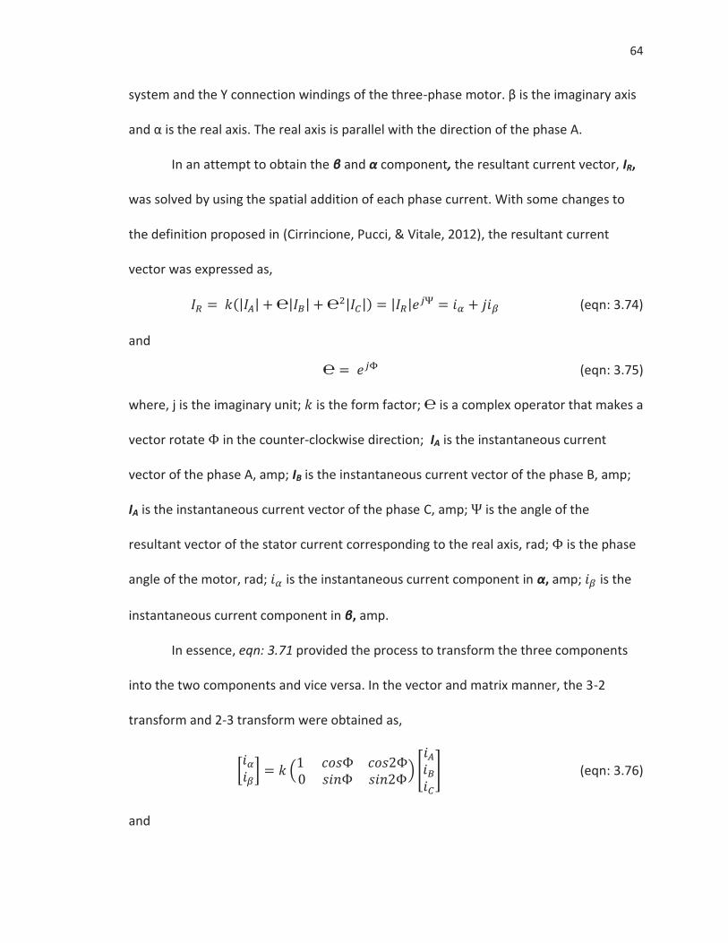
64
system and the Y connection windings of the three-phase motor. β is the imaginary axis
and α is the real axis. The real axis is parallel with the direction of the phase A.
In an attempt to obtain the β and α component, the resultant current vector, IR,
was solved by using the spatial addition of each phase current. With some changes to
the definition proposed in (Cirrincione, Pucci, & Vitale, 2012), the resultant current
vector was expressed as,
(eqn: 3.74)
and
(eqn: 3.75)
where, j is the imaginary unit; is the form factor; is a complex operator that makes a
vector rotate in the counter-clockwise direction; IA is the instantaneous current
vector of the phase A, amp; IB is the instantaneous current vector of the phase B, amp;
IA is the instantaneous current vector of the phase C, amp; is the angle of the
resultant vector of the stator current corresponding to the real axis, rad; is the phase
angle of the motor, rad; is the instantaneous current component in α, amp; is the
instantaneous current component in β, amp.
In essence, eqn: 3.71 provided the process to transform the three components
into the two components and vice versa. In the vector and matrix manner, the 3-2
transform and 2-3 transform were obtained as,
(eqn: 3.76)
and
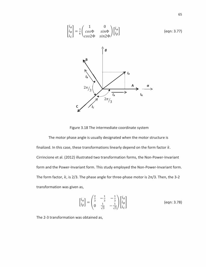
65
(eqn: 3.77)
Figure 3.18 The intermediate coordinate system
The motor phase angle is usually designated when the motor structure is
finalized. In this case, these transformations linearly depend on the form factor .
Cirrincione et al. (2012) illustrated two transformation forms, the Non-Power-Invariant
form and the Power-Invariant form. This study employed the Non-Power-Invariant form.
The form factor, , is 2/3. The phase angle for three-phase motor is 2π/3. Then, the 3-2
transformation was given as,
(eqn: 3.78)
The 2-3 transformation was obtained as,
IR IB
β
IR
α
IC
IA
A
B
C
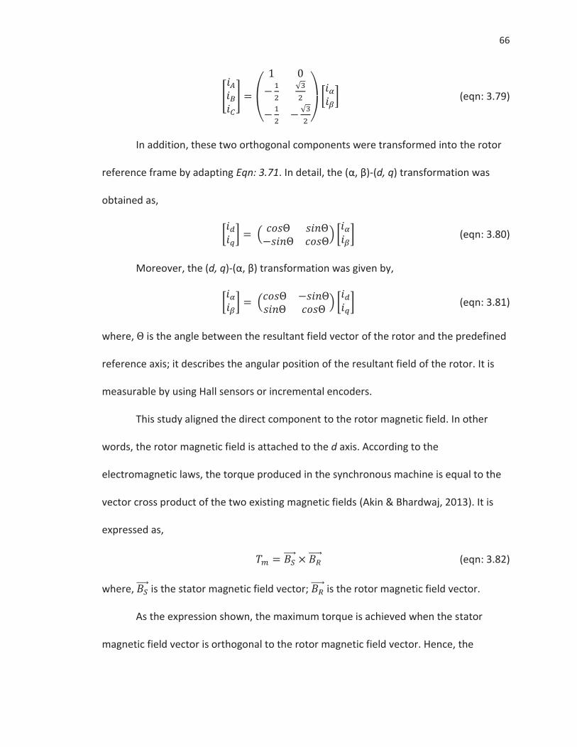
66
(eqn: 3.79)
In addition, these two orthogonal components were transformed into the rotor
reference frame by adapting Eqn: 3.71. In detail, the (α, β)-(d, q) transformation was
obtained as,
(eqn: 3.80)
Moreover, the (d, q)-(α, β) transformation was given by,
(eqn: 3.81)
where, is the angle between the resultant field vector of the rotor and the predefined
reference axis; it describes the angular position of the resultant field of the rotor. It is
measurable by using Hall sensors or incremental encoders.
This study aligned the direct component to the rotor magnetic field. In other
words, the rotor magnetic field is attached to the d axis. According to the
electromagnetic laws, the torque produced in the synchronous machine is equal to the
vector cross product of the two existing magnetic fields (Akin & Bhardwaj, 2013). It is
expressed as,
(eqn: 3.82)
where, is the stator magnetic field vector; is the rotor magnetic field vector.
As the expression shown, the maximum torque is achieved when the stator
magnetic field vector is orthogonal to the rotor magnetic field vector. Hence, the
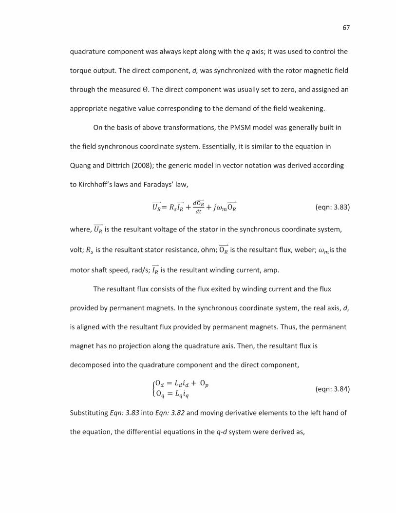
67
quadrature component was always kept along with the q axis; it was used to control the
torque output. The direct component, d, was synchronized with the rotor magnetic field
through the measured . The direct component was usually set to zero, and assigned an
appropriate negative value corresponding to the demand of the field weakening.
On the basis of above transformations, the PMSM model was generally built in
the field synchronous coordinate system. Essentially, it is similar to the equation in
Quang and Dittrich (2008); the generic model in vector notation was derived according
to Kirchhoff’s laws and Faradays’ law,
(eqn: 3.83)
where, is the resultant voltage of the stator in the synchronous coordinate system,
volt; is the resultant stator resistance, ohm; is the resultant flux, weber; is the
motor shaft speed, rad/s; is the resultant winding current, amp.
The resultant flux consists of the flux exited by winding current and the flux
provided by permanent magnets. In the synchronous coordinate system, the real axis, d,
is aligned with the resultant flux provided by permanent magnets. Thus, the permanent
magnet has no projection along the quadrature axis. Then, the resultant flux is
decomposed into the quadrature component and the direct component,
(eqn: 3.84)
Substituting Eqn: 3.83 into Eqn: 3.82 and moving derivative elements to the left hand of
the equation, the differential equations in the q-d system were derived as,
68
(eqn: 3.85)
and
(eqn: 3.86)
where, is the direct axis inductance, H; is the quadrature axis inductance, henry;
is the stator winding resistance, ohm; is the flux produced by the permanent
magnet, weber. The mechanical torque calculation also plays a significant role of the
machine description. The generic torque equation for the PMSM was obtained as,
(eqn: 3.87)
where, is the number of pole pair.
In addition, the motion model of the motor drive was derived as,
(eqn: 3.88)
where, is the motor load, Nm; is the total equivalent inertia of tire, gear set and
motor shaft, kg·m2; is the damping of the motor drive, Nm/(rad/s).
The dynamic transition characteristic of the system was integrated into the total
equivalent inertia. The motor load was approximated as a constant value over one
sample step; it was updated at each execution cycle. Considering the drag force and
grading fore of the vehicle, was represented by,
(eqn: 3.89)
where, is the reduction gear ratio; is the effective propulsion factor, which is
equal to the number of effective motors.
69
In summary, the three-phase motor system was represented in state space form,
(eqn: 3.90)
and
; ; (eqn: 3.91)
and then rewrite the Eqn: 3.8 into vector form as,
(eqn: 3.92)
where, is the system matrix of the motor process; is the input matrix of the
motor process; is the bilinear coupling matrix of the motor process; is the
disturbance vector of the motor process.
3.2.2.2 Battery Modeling
This research investigated the terminal voltage, the battery temperature and
state of charge (SOC) of the selected battery. The model mainly consists of two sub-
models, the terminal voltage sub-model and SOC sub-model. The terminal voltage sub-
model covered five primary battery effects. The battery thermal model was created
according to the conservation of energy and the heat transfer principle. The SOC was
calculated according to the battery current, the nominal battery cell capacity and the
initial SOC. Figure 3.19 illustrates that the internal resistance, inductance, double layer
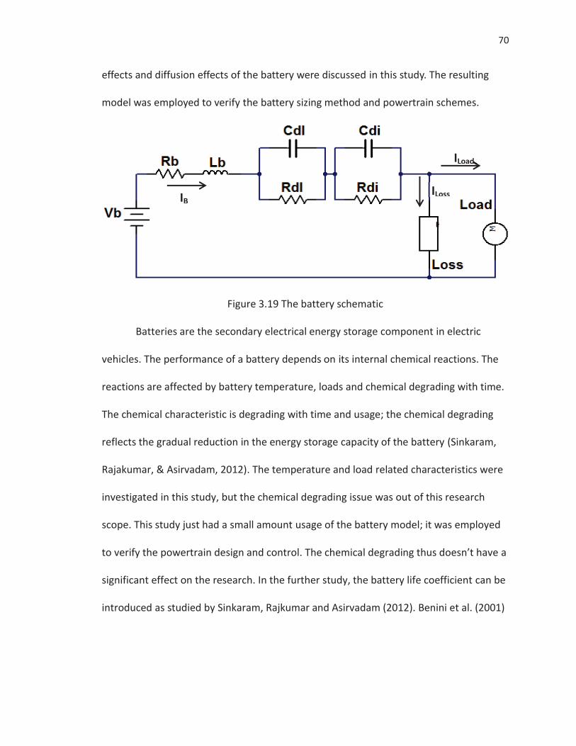
70
effects and diffusion effects of the battery were discussed in this study. The resulting
model was employed to verify the battery sizing method and powertrain schemes.
Figure 3.19 The battery schematic
Batteries are the secondary electrical energy storage component in electric
vehicles. The performance of a battery depends on its internal chemical reactions. The
reactions are affected by battery temperature, loads and chemical degrading with time.
The chemical characteristic is degrading with time and usage; the chemical degrading
reflects the gradual reduction in the energy storage capacity of the battery (Sinkaram,
Rajakumar, & Asirvadam, 2012). The temperature and load related characteristics were
investigated in this study, but the chemical degrading issue was out of this research
scope. This study just had a small amount usage of the battery model; it was employed
to verify the powertrain design and control. The chemical degrading thus doesn’t have a
significant effect on the research. In the further study, the battery life coefficient can be
introduced as studied by Sinkaram, Rajkumar and Asirvadam (2012). Benini et al. (2001)
IB
ILoad
ILoss
71
also researched a battery lifetime model that considering the effects of the average
current and the profile of the current waveform in time domain.
3.2.2.2.1 Terminal Voltage
The battery terminal voltage was calculated on the basis of the open circuit
voltage, voltage drop due to the battery internal resistance, capacitance, inductance
and the temperature impact on the battery potential. With some adjustments to
formulations in Gao, Liu and Dougal (2002), the battery output voltage was computed
as,
(eqn: 3.93)
where, is the battery terminal voltage, volt; is the battery electromotive force
voltage, volt; is the battery internal voltage loss, volt. The electromotive force voltage
is a function of the SOC. It was given as,
(eqn: 3.94)
where, is the amount of cells in series; is the electromotive force of the battery
cell, volt.
Furthermore, this study introduced the calculation of the electromotive force of
the battery cell as presented in Chen and Mora (2006). It was given as,
(eqn: 3.95)
The internal voltage loss is due to the battery internal resistance, the double
layer effect and the diffusion effect. The equivalent diagram was presented in Figure
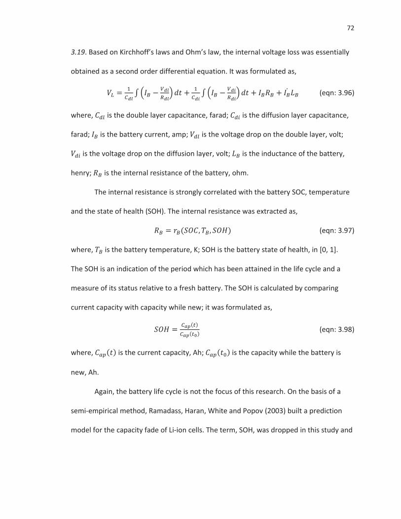
72
3.19. Based on Kirchhoff’s laws and Ohm’s law, the internal voltage loss was essentially
obtained as a second order differential equation. It was formulated as,
(eqn: 3.96)
where, is the double layer capacitance, farad; is the diffusion layer capacitance,
farad; is the battery current, amp; is the voltage drop on the double layer, volt;
is the voltage drop on the diffusion layer, volt; is the inductance of the battery,
henry; is the internal resistance of the battery, ohm.
The internal resistance is strongly correlated with the battery SOC, temperature
and the state of health (SOH). The internal resistance was extracted as,
(eqn: 3.97)
where, is the battery temperature, K; SOH is the battery state of health, in [0, 1].
The SOH is an indication of the period which has been attained in the life cycle and a
measure of its status relative to a fresh battery. The SOH is calculated by comparing
current capacity with capacity while new; it was formulated as,
(eqn: 3.98)
where, is the current capacity, Ah; is the capacity while the battery is
new, Ah.
Again, the battery life cycle is not the focus of this research. On the basis of a
semi-empirical method, Ramadass, Haran, White and Popov (2003) built a prediction
model for the capacity fade of Li-ion cells. The term, SOH, was dropped in this study and
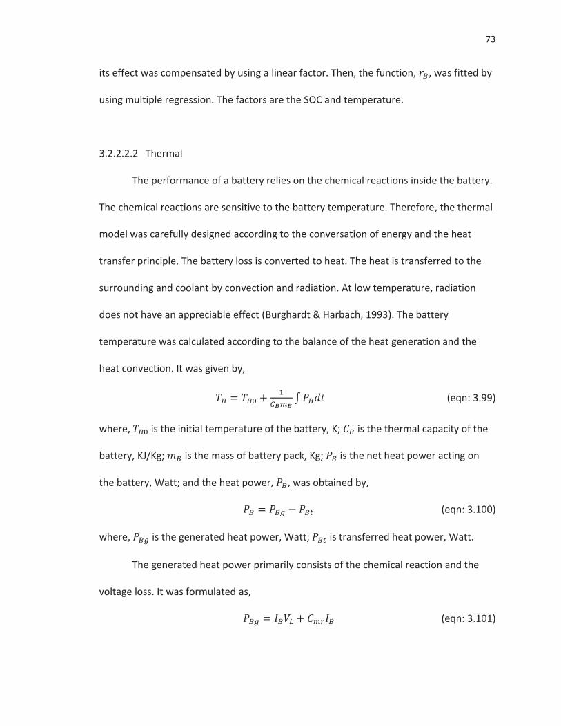
73
its effect was compensated by using a linear factor. Then, the function, , was fitted by
using multiple regression. The factors are the SOC and temperature.
3.2.2.2.2 Thermal
The performance of a battery relies on the chemical reactions inside the battery.
The chemical reactions are sensitive to the battery temperature. Therefore, the thermal
model was carefully designed according to the conversation of energy and the heat
transfer principle. The battery loss is converted to heat. The heat is transferred to the
surrounding and coolant by convection and radiation. At low temperature, radiation
does not have an appreciable effect (Burghardt & Harbach, 1993). The battery
temperature was calculated according to the balance of the heat generation and the
heat convection. It was given by,
(eqn: 3.99)
where, is the initial temperature of the battery, K; is the thermal capacity of the
battery, KJ/Kg; is the mass of battery pack, Kg; is the net heat power acting on
the battery, Watt; and the heat power, , was obtained by,
(eqn: 3.100)
where, is the generated heat power, Watt; is transferred heat power, Watt.
The generated heat power primarily consists of the chemical reaction and the
voltage loss. It was formulated as,
(eqn: 3.101)
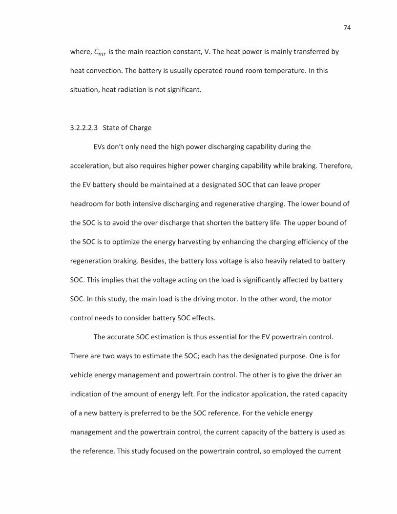
74
where, is the main reaction constant, V. The heat power is mainly transferred by
heat convection. The battery is usually operated round room temperature. In this
situation, heat radiation is not significant.
3.2.2.2.3 State of Charge
EVs don’t only need the high power discharging capability during the
acceleration, but also requires higher power charging capability while braking. Therefore,
the EV battery should be maintained at a designated SOC that can leave proper
headroom for both intensive discharging and regenerative charging. The lower bound of
the SOC is to avoid the over discharge that shorten the battery life. The upper bound of
the SOC is to optimize the energy harvesting by enhancing the charging efficiency of the
regeneration braking. Besides, the battery loss voltage is also heavily related to battery
SOC. This implies that the voltage acting on the load is significantly affected by battery
SOC. In this study, the main load is the driving motor. In the other word, the motor
control needs to consider battery SOC effects.
The accurate SOC estimation is thus essential for the EV powertrain control.
There are two ways to estimate the SOC; each has the designated purpose. One is for
vehicle energy management and powertrain control. The other is to give the driver an
indication of the amount of energy left. For the indicator application, the rated capacity
of a new battery is preferred to be the SOC reference. For the vehicle energy
management and the powertrain control, the current capacity of the battery is used as
the reference. This study focused on the powertrain control, so employed the current
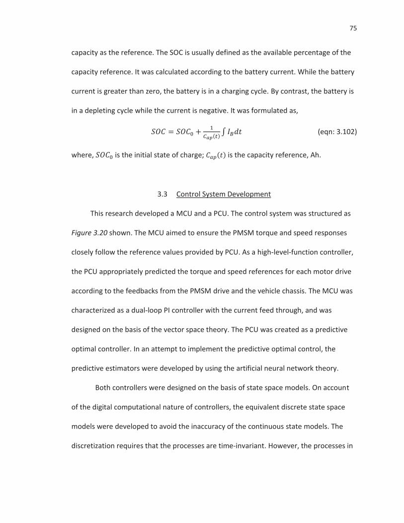
75
capacity as the reference. The SOC is usually defined as the available percentage of the
capacity reference. It was calculated according to the battery current. While the battery
current is greater than zero, the battery is in a charging cycle. By contrast, the battery is
in a depleting cycle while the current is negative. It was formulated as,
(eqn: 3.102)
where, is the initial state of charge; is the capacity reference, Ah.
3.3 Control System Development
This research developed a MCU and a PCU. The control system was structured as
Figure 3.20 shown. The MCU aimed to ensure the PMSM torque and speed responses
closely follow the reference values provided by PCU. As a high-level-function controller,
the PCU appropriately predicted the torque and speed references for each motor drive
according to the feedbacks from the PMSM drive and the vehicle chassis. The MCU was
characterized as a dual-loop PI controller with the current feed through, and was
designed on the basis of the vector space theory. The PCU was created as a predictive
optimal controller. In an attempt to implement the predictive optimal control, the
predictive estimators were developed by using the artificial neural network theory.
Both controllers were designed on the basis of state space models. On account
of the digital computational nature of controllers, the equivalent discrete state space
models were developed to avoid the inaccuracy of the continuous state models. The
discretization requires that the processes are time-invariant. However, the processes in
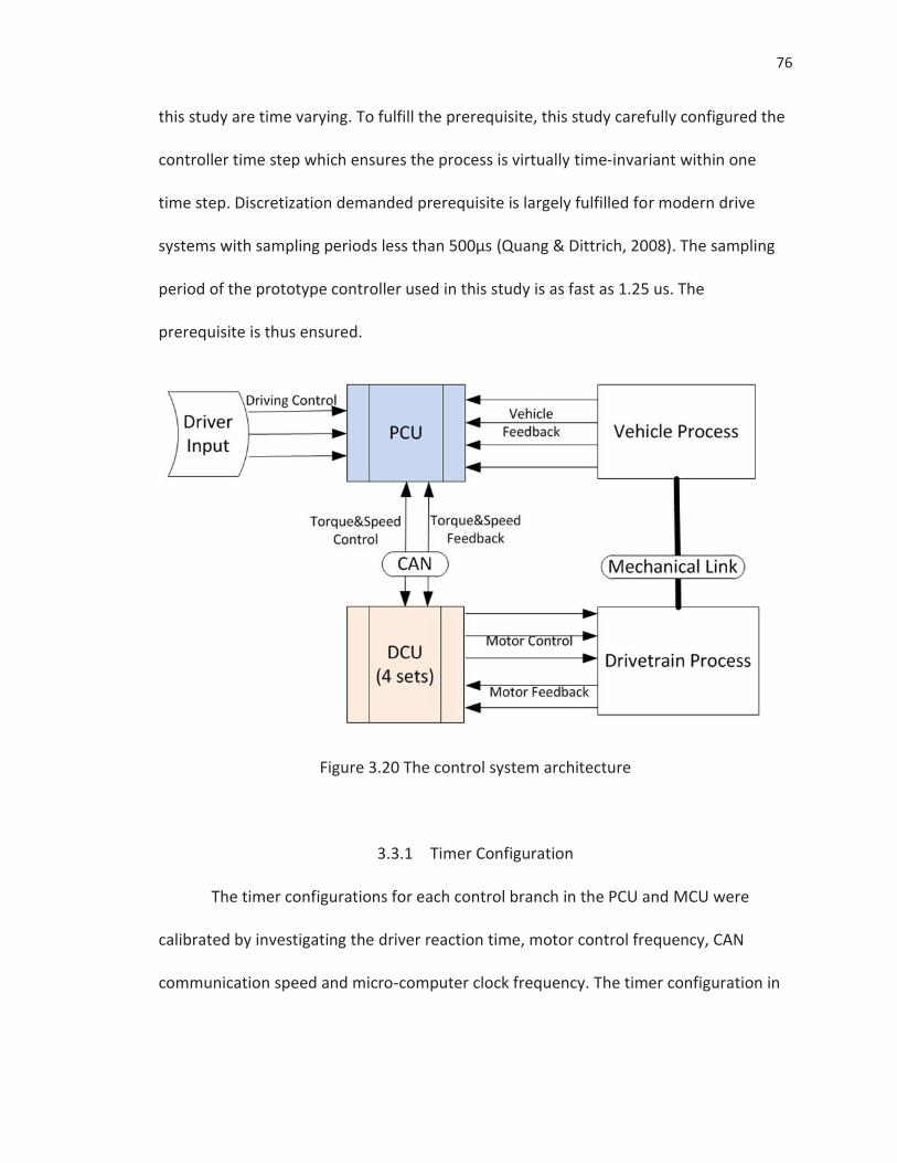
76
this study are time varying. To fulfill the prerequisite, this study carefully configured the
controller time step which ensures the process is virtually time-invariant within one
time step. Discretization demanded prerequisite is largely fulfilled for modern drive
systems with sampling periods less than 500μs (Quang & Dittrich, 2008). The sampling
period of the prototype controller used in this study is as fast as 1.25 us. The
prerequisite is thus ensured.
Figure 3.20 The control system architecture
3.3.1 Timer Configuration
The timer configurations for each control branch in the PCU and MCU were
calibrated by investigating the driver reaction time, motor control frequency, CAN
communication speed and micro-computer clock frequency. The timer configuration in
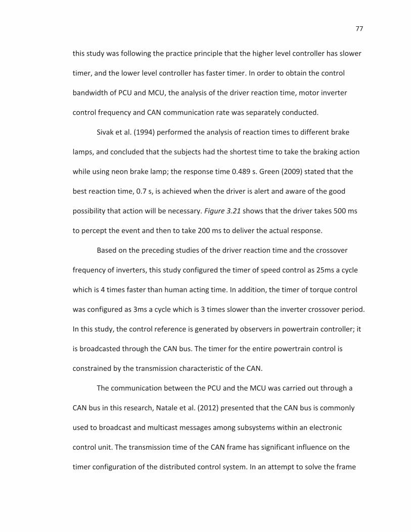
77
this study was following the practice principle that the higher level controller has slower
timer, and the lower level controller has faster timer. In order to obtain the control
bandwidth of PCU and MCU, the analysis of the driver reaction time, motor inverter
control frequency and CAN communication rate was separately conducted.
Sivak et al. (1994) performed the analysis of reaction times to different brake
lamps, and concluded that the subjects had the shortest time to take the braking action
while using neon brake lamp; the response time 0.489 s. Green (2009) stated that the
best reaction time, 0.7 s, is achieved when the driver is alert and aware of the good
possibility that action will be necessary. Figure 3.21 shows that the driver takes 500 ms
to percept the event and then to take 200 ms to deliver the actual response.
Based on the preceding studies of the driver reaction time and the crossover
frequency of inverters, this study configured the timer of speed control as 25ms a cycle
which is 4 times faster than human acting time. In addition, the timer of torque control
was configured as 3ms a cycle which is 3 times slower than the inverter crossover period.
In this study, the control reference is generated by observers in powertrain controller; it
is broadcasted through the CAN bus. The timer for the entire powertrain control is
constrained by the transmission characteristic of the CAN.
The communication between the PCU and the MCU was carried out through a
CAN bus in this research, Natale et al. (2012) presented that the CAN bus is commonly
used to broadcast and multicast messages among subsystems within an electronic
control unit. The transmission time of the CAN frame has significant influence on the
timer configuration of the distributed control system. In an attempt to solve the frame
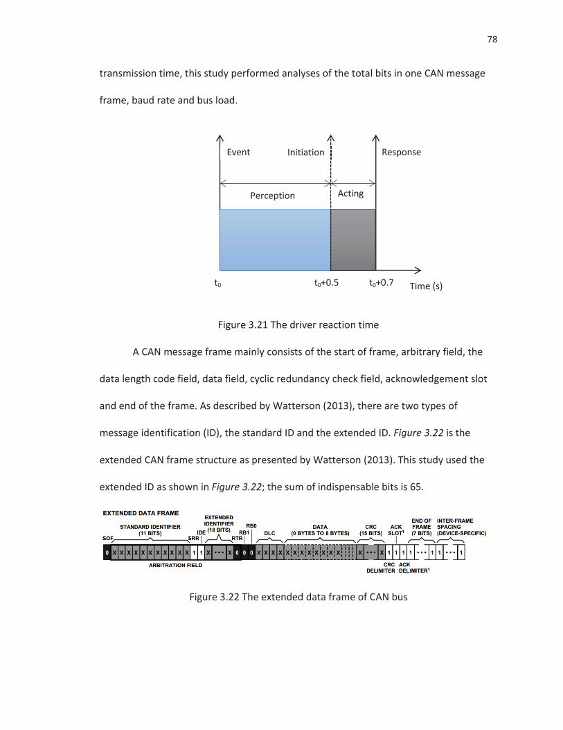
78
transmission time, this study performed analyses of the total bits in one CAN message
frame, baud rate and bus load.
Figure 3.21 The driver reaction time
A CAN message frame mainly consists of the start of frame, arbitrary field, the
data length code field, data field, cyclic redundancy check field, acknowledgement slot
and end of the frame. As described by Watterson (2013), there are two types of
message identification (ID), the standard ID and the extended ID. Figure 3.22 is the
extended CAN frame structure as presented by Watterson (2013). This study used the
extended ID as shown in Figure 3.22; the sum of indispensable bits is 65.
Figure 3.22 The extended data frame of CAN bus
Event
Time (s)
Response
Perception
Initiation
Acting
t0 t0+0.5 t0+0.7
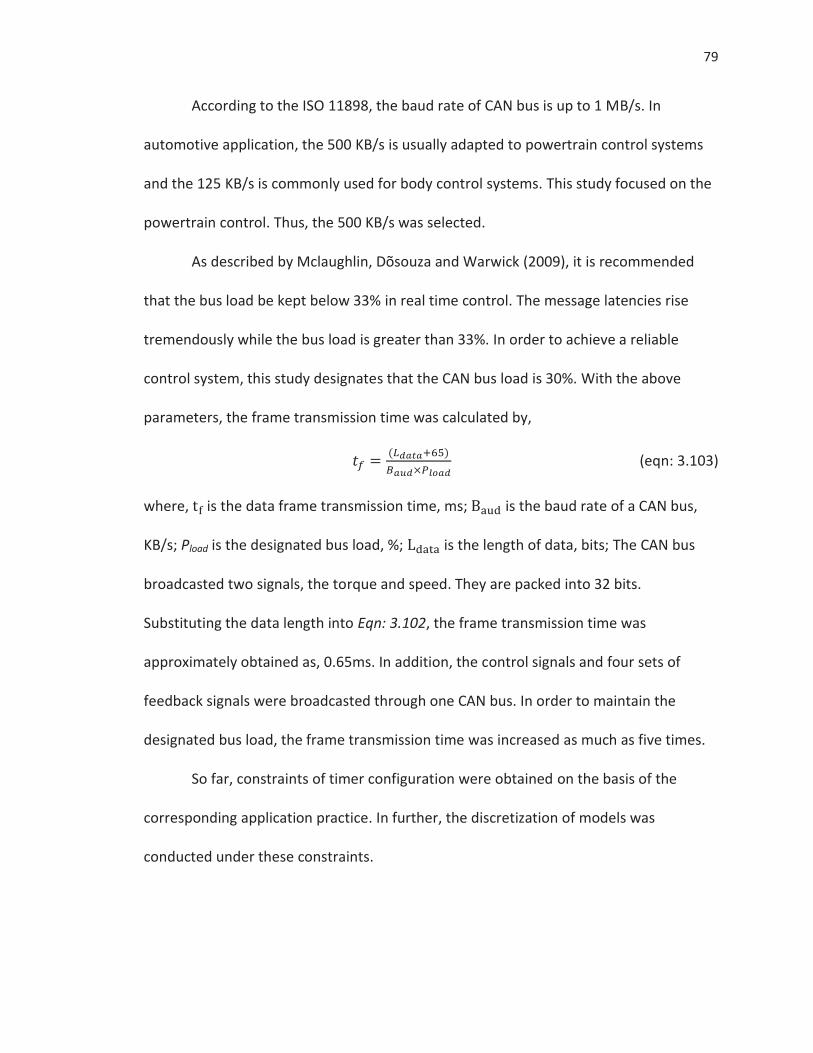
79
According to the ISO 11898, the baud rate of CAN bus is up to 1 MB/s. In
automotive application, the 500 KB/s is usually adapted to powertrain control systems
and the 125 KB/s is commonly used for body control systems. This study focused on the
powertrain control. Thus, the 500 KB/s was selected.
As described by Mclaughlin, Dõsouza and Warwick (2009), it is recommended
that the bus load be kept below 33% in real time control. The message latencies rise
tremendously while the bus load is greater than 33%. In order to achieve a reliable
control system, this study designates that the CAN bus load is 30%. With the above
parameters, the frame transmission time was calculated by,
(eqn: 3.103)
where, is the data frame transmission time, ms; is the baud rate of a CAN bus,
KB/s; Pload is the designated bus load, %; is the length of data, bits; The CAN bus
broadcasted two signals, the torque and speed. They are packed into 32 bits.
Substituting the data length into Eqn: 3.102, the frame transmission time was
approximately obtained as, 0.65ms. In addition, the control signals and four sets of
feedback signals were broadcasted through one CAN bus. In order to maintain the
designated bus load, the frame transmission time was increased as much as five times.
So far, constraints of timer configuration were obtained on the basis of the
corresponding application practice. In further, the discretization of models was
conducted under these constraints.
80
3.3.2 Model Parameterization and Discretization
To support the controller development, this research substituted the well-
defined parameters into the generic models derived in above sections, and transferred
the process model and observers into discrete model according to digital processing
principles. In control systems, it is necessary to observe the work of the controlled
object (Zumbahlen, 2007).
Historically, the control system was analog. Therefore, even today, plenty of
computer-based control systems are still using continuous transfer functions. In essence,
the microcomputer is a digital device. It works discretely and processes responses are
sampled in discrete time tick. The continuous state transfer functions aren’t sufficient
anymore. Quang and Dittrich (2008) emphasized that the sampling can cause the special
phenomena, which needs to be considered in the design. Thus, it is necessary to
develop the discrete models of motor and vehicle dynamic for the further controller
development. As described by Quang and Dittrich (2008), there are two alternatives to
obtain the discrete models:
1. Design the controller for the continuous system and just discretize its
implementation.
2. Develop the discrete controller on the basis of the discrete process.
The first manner is also called as quasi-continuous design, which has limitations
to eliminate inherent defects from the continuous design. The second method was
employed by this research. The equivalent discrete models were obtained by converting
the derived continuous state space models. The discrete state model was derived on the
81
basis of the generic solution of the continuous state equation for the linear time-variant
system in which the matrix A and B depend on time. With some changes to the equation
described by Quang and Dittrich (2008), the generic solution was given by,
(eqn: 3.104)
where, is the transition matrix of the system from X(t0) to X(t) following the
trajectory, . The matrix follows the prerequisite as was given by,
(eqn: 3.105)
If the system matrix, A(t), keeps constant over one sample step, the analytical
solution of the transition matrix can be obtained as a matrix exponential function,
(eqn: 3.106)
Substituting Eqn: 3.105 into the Eqn: 3.103 and taking the integration over one
sample step, the equation was rewritten in the notion of discrete time tick as,
(eqn: 3.107)
where,
(eqn: 3.108)
A and B are just secured as constant over one sampling time. In principle, they are
varied with respect to kT. Therefore, the discrete system matrix, A(kT), and the discrete
input matrix, B(kT), have to be recomputed at each sampling period. So far, a time-
variant discrete system is derived.
82
Furthermore, the input vector, u(t), holds the same value for one sampling step,
because it is usually discretized by a zero-order hold function. Thus, u(t) was extracted
from the integral term. Eqn: 3.106 was rewritten as,
(eqn: 3.109)
where,
(eqn: 3.110)
and
(eqn: 3.111)
and, in further, is solved as,
(eqn: 3.112)
In analogy to the continuous state space equations, the system output was
represented as,
(eqn: 3.113)
where, is the output matrix of the system; is the feed-through matrix of
control vector.
As the primary component of the discretization process, has significant
impact on the dynamics and stability of the discrete system. should converge in
the transition process. There are various manners to approximately evaluate . In
the real time applications, the series expansion and equivalent function are commonly
used. With the series expansion method, Eqn: 3.109 is expanded into a power series. It
is formulated as,
83
(eqn: 3.114)
To fulfill the stability requirements, the eigenvalues of the system must follow
the inequality as is given by,
(eqn: 3.115)
Using the equivalent function method, the matrix function is recreated by an
equivalent polynomial function as described by Quang and Dittrich (2008). It is
represented by,
(eqn: 3.116)
where, n is the order of the system matrix; is the estimation factor of the polynomial
method, which can be solved by the Sylvester-Lagrange equivalent polynomial method.
So far, the generic discrete representation was obtained for linear time-variant systems.
By contrast, there is no method to achieve an equivalent discrete system for nonlinear
and time-variant systems. However, if the continuous system is bilinear, the equivalent
discrete representation is achievable. The system can be formulated as,
(eqn: 3.117)
where, is the coupling matrix.
For this system, and of the equivalent discrete system was solved as,
(eqn: 3.118)
and
(eqn: 3.119)
84
To summarize, the generic discretization procedure for linear time-variant and
bilinear systems was obtained. In further, this study created discrete models of the
motor and vehicle dynamic by adapting this generic procedure.
3.3.2.1 Motor Discrete Model
In the q-d coordinate system, the continuous state space model of the three-
phase PMSM was obtained as Eqn: 3.91. The coupling matrix implicitly depends on the
control input. Besides, the permanent magnetic flux is correlated to the motor
operation temperature. The temperature is a slowly varying process. Thus, this research
appropriately assumed that the permanent magnetic flux, , is constant over at least
one sample time. According to the generic form of discretization in the previous section,
this research reshaped Eqn: 3.91 into the following form,
(eqn: 3.120)
where,
; (eqn: 3.121)
and, in further, the discrete model of the three-phase PMSM was obtained as,
(eqn: 3.122)
where, and was solved by using the series expansion method. They were given
as,
(eqn: 3.123)
and
85
(eqn: 3.124)
and took the first order approximation for the transition matrix, , and the input
matrix, , and then solved them as,
(eqn: 3.125)
and
(eqn: 3.126)
where, was partitioned into . The inverse of was used to design a
feed-forward controller to compensate the permanent magnetic flux.
3.3.2.2 Vehicle Dynamic Discrete Model
This research had investigated the yaw dynamics, roll dynamics and longitudinal
dynamics in previous sections. For the controller development point of view, this
research focused on the yaw dynamics. The states of roll dynamics and longitudinal
dynamics were functioning as the disturbance and the coupling terms. What is more,
the load transfer due to roll movement is the main disturbance to the system in yaw
plane. The longitudinal velocity is the coupling term of the system which depends on the
control input. As given in Eqn: 3.58 and Eqn: 3.59, the system matrix doesn’t only
include time-invariant terms, but also the time-variant terms and coupling terms. Thus,
86
the system in yaw plane is a typical bilinear system. It was discretized in analogy to the
discretization of the PMSM model. The equation was reshaped as,
(eqn: 3.127)
where,
; (eqn: 3.128)
In further, the discrete model of the vehicle dynamic model in yaw plane was
obtained as,
(eqn: 3.129)
where, and was solved by using the series expansion method. They were given as,
(eqn: 3.130)
and
(eqn: 3.131)
So far, the discrete models of the PMSM and yaw dynamics were obtained. The
motor controller and powertrain controller were developed and analyzed on the basis
of these models in the following sections.
3.3.3 Motor Control
In general, the vector control method was employed by this research to control
the three-phase PMSM. By using the vector control theory, the three-phase motor was
transformed to an excited DC motor as discussed in the motor modeling section. Thus,
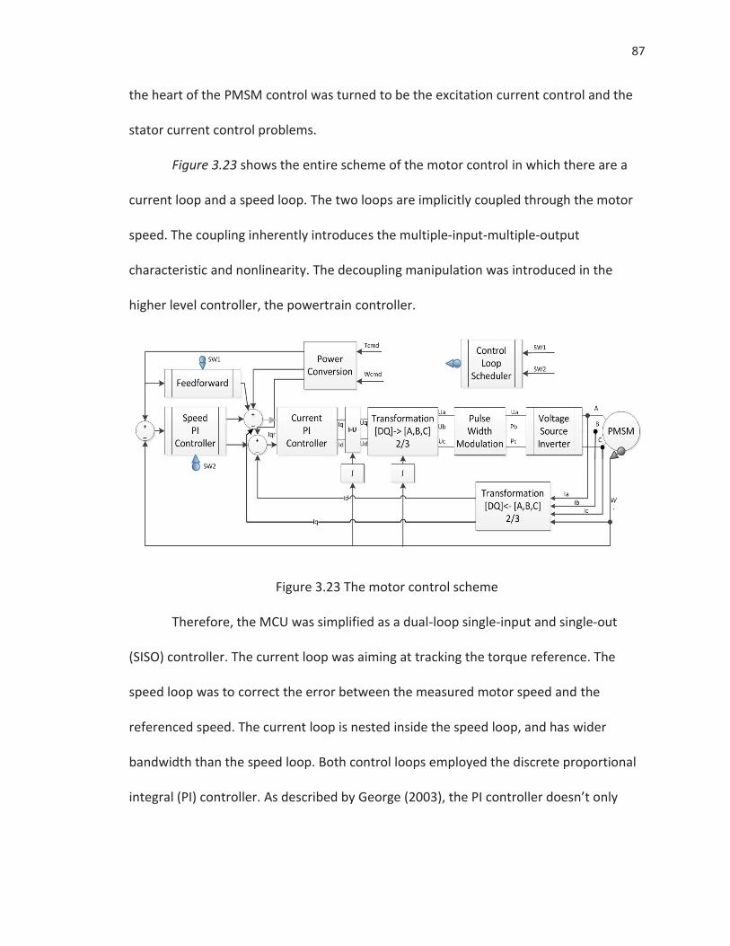
87
the heart of the PMSM control was turned to be the excitation current control and the
stator current control problems.
Figure 3.23 shows the entire scheme of the motor control in which there are a
current loop and a speed loop. The two loops are implicitly coupled through the motor
speed. The coupling inherently introduces the multiple-input-multiple-output
characteristic and nonlinearity. The decoupling manipulation was introduced in the
higher level controller, the powertrain controller.
Figure 3.23 The motor control scheme
Therefore, the MCU was simplified as a dual-loop single-input and single-out
(SISO) controller. The current loop was aiming at tracking the torque reference. The
speed loop was to correct the error between the measured motor speed and the
referenced speed. The current loop is nested inside the speed loop, and has wider
bandwidth than the speed loop. Both control loops employed the discrete proportional
integral (PI) controller. As described by George (2003), the PI controller doesn’t only
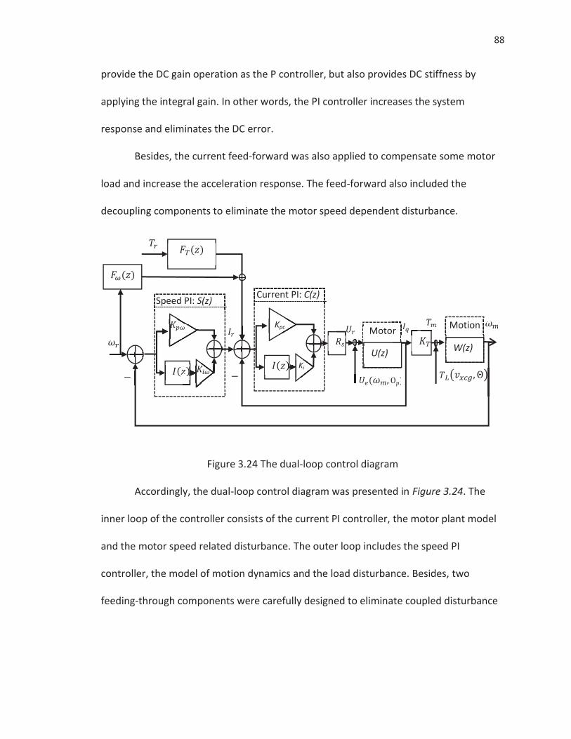
88
provide the DC gain operation as the P controller, but also provides DC stiffness by
applying the integral gain. In other words, the PI controller increases the system
response and eliminates the DC error.
Besides, the current feed-forward was also applied to compensate some motor
load and increase the acceleration response. The feed-forward also included the
decoupling components to eliminate the motor speed dependent disturbance.
Figure 3.24 The dual-loop control diagram
Accordingly, the dual-loop control diagram was presented in Figure 3.24. The
inner loop of the controller consists of the current PI controller, the motor plant model
and the motor speed related disturbance. The outer loop includes the speed PI
controller, the model of motion dynamics and the load disturbance. Besides, two
feeding-through components were carefully designed to eliminate coupled disturbance
Kpc
Ki
W(z)
Current PI: C(z)
Motion
U(z)
Motor
Speed PI: S(z)
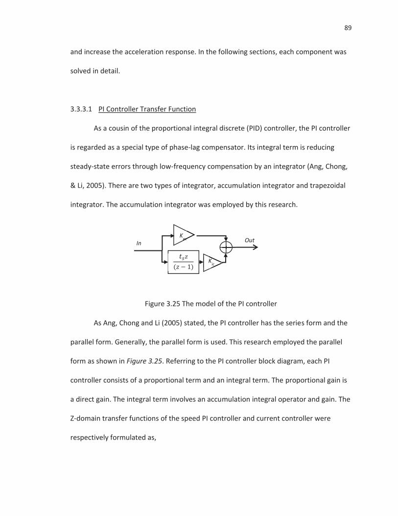
89
and increase the acceleration response. In the following sections, each component was
solved in detail.
3.3.3.1 PI Controller Transfer Function
As a cousin of the proportional integral discrete (PID) controller, the PI controller
is regarded as a special type of phase-lag compensator. Its integral term is reducing
steady-state errors through low-frequency compensation by an integrator (Ang, Chong,
& Li, 2005). There are two types of integrator, accumulation integrator and trapezoidal
integrator. The accumulation integrator was employed by this research.
Figure 3.25 The model of the PI controller
As Ang, Chong and Li (2005) stated, the PI controller has the series form and the
parallel form. Generally, the parallel form is used. This research employed the parallel
form as shown in Figure 3.25. Referring to the PI controller block diagram, each PI
controller consists of a proportional term and an integral term. The proportional gain is
a direct gain. The integral term involves an accumulation integral operator and gain. The
Z-domain transfer functions of the speed PI controller and current controller were
respectively formulated as,
Kpc
Kic
In Out
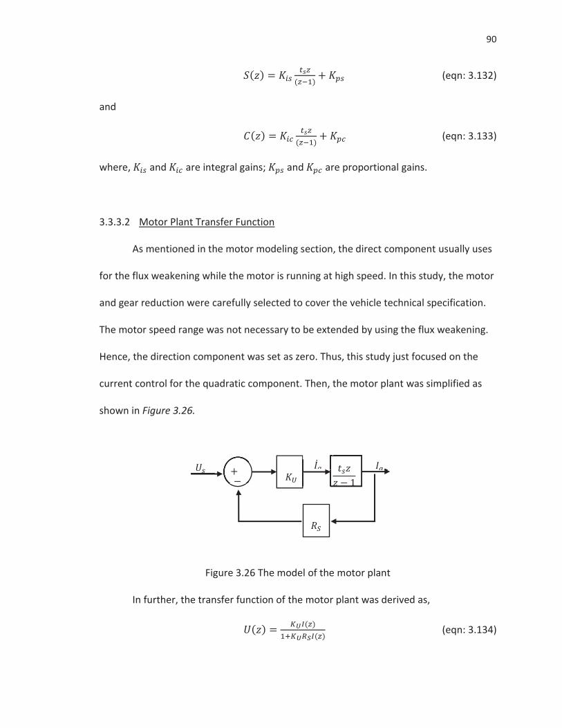
90
(eqn: 3.132)
and
(eqn: 3.133)
where, and are integral gains; and are proportional gains.
3.3.3.2 Motor Plant Transfer Function
As mentioned in the motor modeling section, the direct component usually uses
for the flux weakening while the motor is running at high speed. In this study, the motor
and gear reduction were carefully selected to cover the vehicle technical specification.
The motor speed range was not necessary to be extended by using the flux weakening.
Hence, the direction component was set as zero. Thus, this study just focused on the
current control for the quadratic component. Then, the motor plant was simplified as
shown in Figure 3.26.
Figure 3.26 The model of the motor plant
In further, the transfer function of the motor plant was derived as,
(eqn: 3.134)
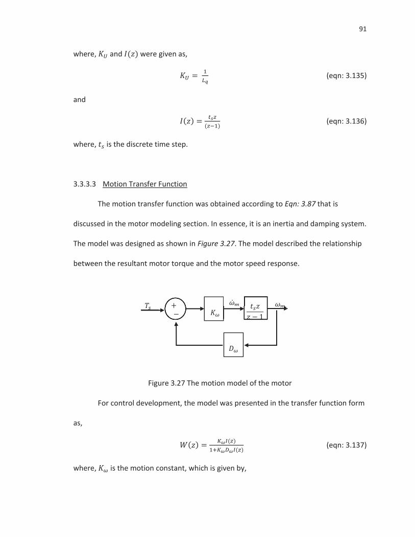
91
where, and were given as,
(eqn: 3.135)
and
(eqn: 3.136)
where, is the discrete time step.
3.3.3.3 Motion Transfer Function
The motion transfer function was obtained according to Eqn: 3.87 that is
discussed in the motor modeling section. In essence, it is an inertia and damping system.
The model was designed as shown in Figure 3.27. The model described the relationship
between the resultant motor torque and the motor speed response.
Figure 3.27 The motion model of the motor
For control development, the model was presented in the transfer function form
as,
(eqn: 3.137)
where, is the motion constant, which is given by,
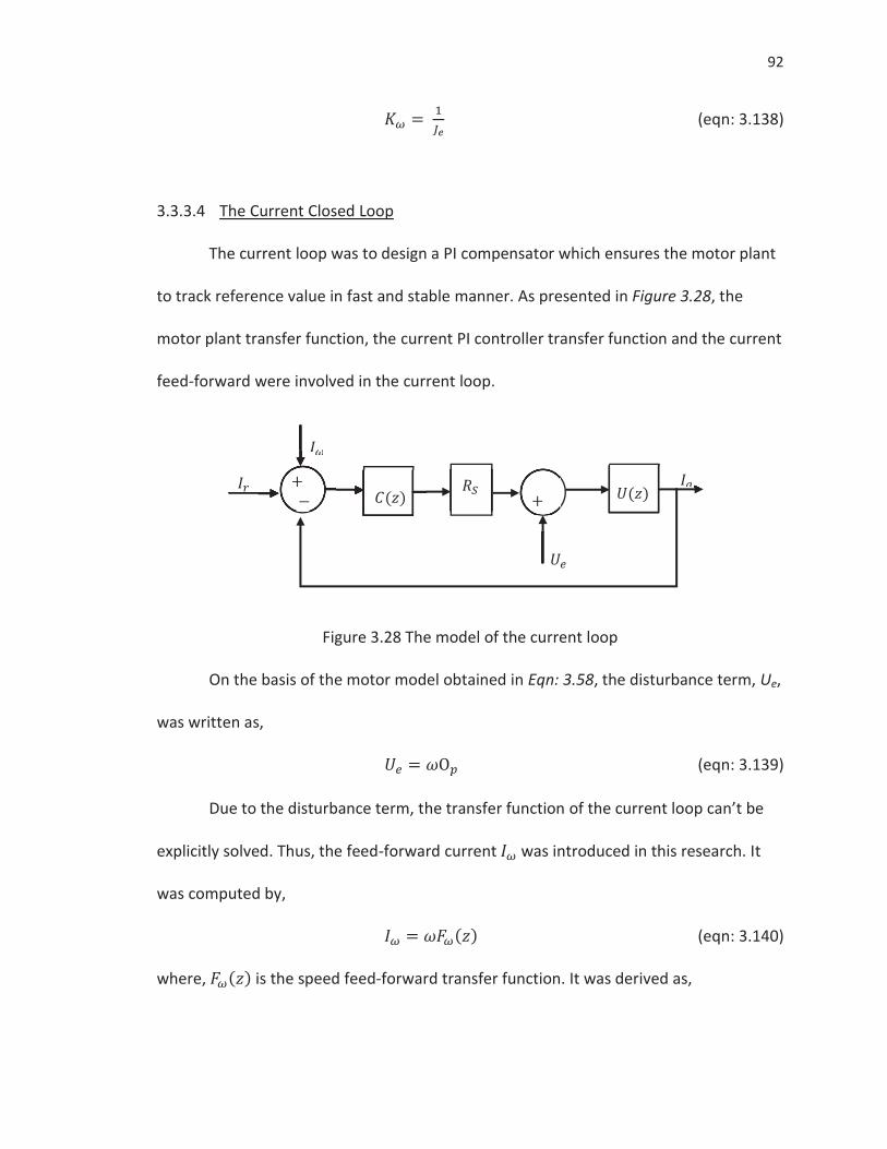
92
(eqn: 3.138)
3.3.3.4 The Current Closed Loop
The current loop was to design a PI compensator which ensures the motor plant
to track reference value in fast and stable manner. As presented in Figure 3.28, the
motor plant transfer function, the current PI controller transfer function and the current
feed-forward were involved in the current loop.
Figure 3.28 The model of the current loop
On the basis of the motor model obtained in Eqn: 3.58, the disturbance term, Ue,
was written as,
(eqn: 3.139)
Due to the disturbance term, the transfer function of the current loop can’t be
explicitly solved. Thus, the feed-forward current was introduced in this research. It
was computed by,
(eqn: 3.140)
where, is the speed feed-forward transfer function. It was derived as,
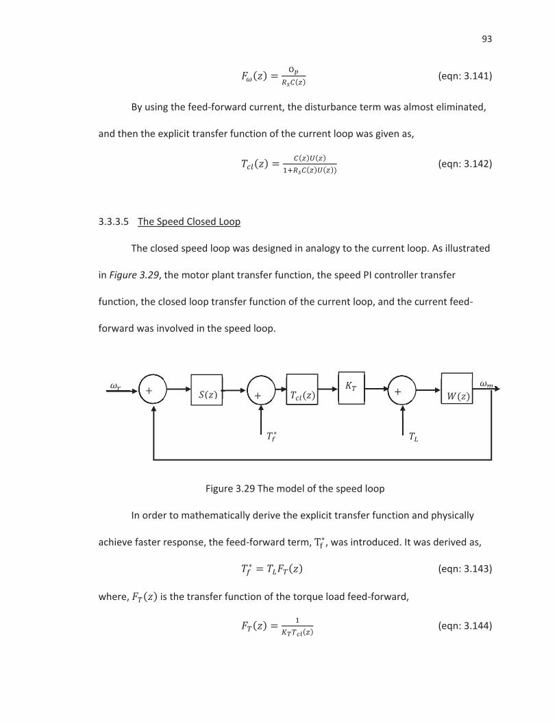
93
(eqn: 3.141)
By using the feed-forward current, the disturbance term was almost eliminated,
and then the explicit transfer function of the current loop was given as,
(eqn: 3.142)
3.3.3.5 The Speed Closed Loop
The closed speed loop was designed in analogy to the current loop. As illustrated
in Figure 3.29, the motor plant transfer function, the speed PI controller transfer
function, the closed loop transfer function of the current loop, and the current feed-
forward was involved in the speed loop.
Figure 3.29 The model of the speed loop
In order to mathematically derive the explicit transfer function and physically
achieve faster response, the feed-forward term, , was introduced. It was derived as,
(eqn: 3.143)
where, is the transfer function of the torque load feed-forward,
(eqn: 3.144)
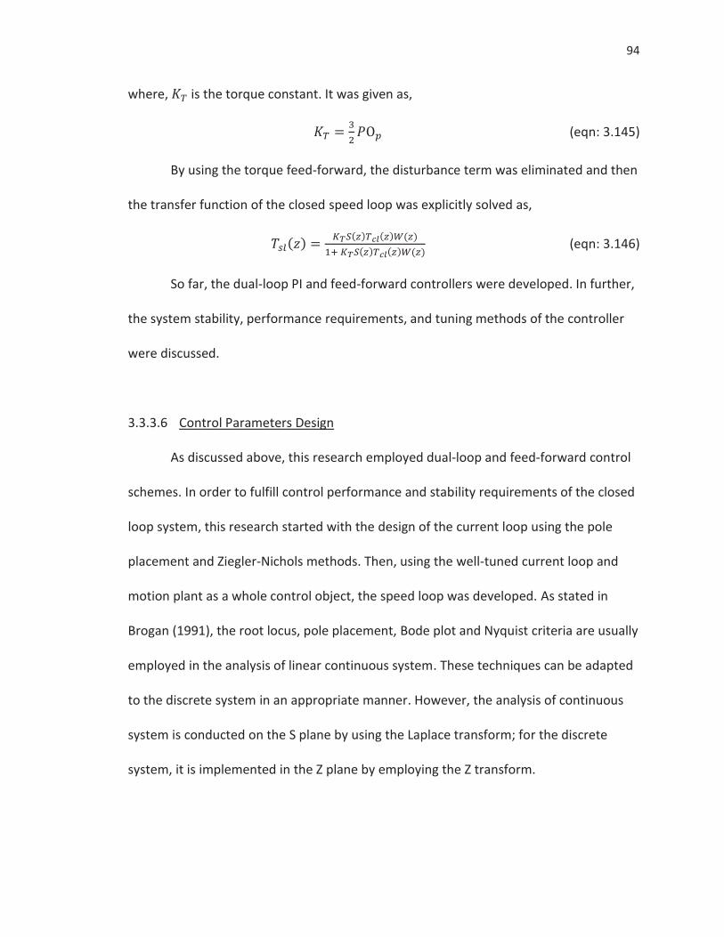
94
where, is the torque constant. It was given as,
(eqn: 3.145)
By using the torque feed-forward, the disturbance term was eliminated and then
the transfer function of the closed speed loop was explicitly solved as,
(eqn: 3.146)
So far, the dual-loop PI and feed-forward controllers were developed. In further,
the system stability, performance requirements, and tuning methods of the controller
were discussed.
3.3.3.6 Control Parameters Design
As discussed above, this research employed dual-loop and feed-forward control
schemes. In order to fulfill control performance and stability requirements of the closed
loop system, this research started with the design of the current loop using the pole
placement and Ziegler-Nichols methods. Then, using the well-tuned current loop and
motion plant as a whole control object, the speed loop was developed. As stated in
Brogan (1991), the root locus, pole placement, Bode plot and Nyquist criteria are usually
employed in the analysis of linear continuous system. These techniques can be adapted
to the discrete system in an appropriate manner. However, the analysis of continuous
system is conducted on the S plane by using the Laplace transform; for the discrete
system, it is implemented in the Z plane by employing the Z transform.
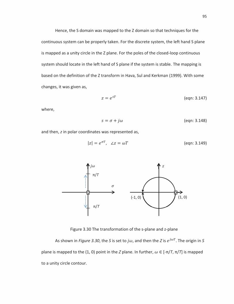
95
Hence, the S domain was mapped to the Z domain so that techniques for the
continuous system can be properly taken. For the discrete system, the left hand S plane
is mapped as a unity circle in the Z plane. For the poles of the closed-loop continuous
system should locate in the left hand of S plane if the system is stable. The mapping is
based on the definition of the Z transform in Hava, Sul and Kerkman (1999). With some
changes, it was given as,
(eqn: 3.147)
where,
(eqn: 3.148)
and then, z in polar coordinates was represented as,
(eqn: 3.149)
Figure 3.30 The transformation of the s-plane and z-plane
As shown in Figure 3.30, the S is set to , and then the Z is The origin in S
plane is mapped to the (1, 0) point in the Z plane. In further, [-π/T, π/T] is mapped
to a unity circle contour.
π/T
π/T
(1, 0) (-1, 0)

96
Figure 3.31 The transformation of the primary pole
In order to achieve the specified requirements of the settling time, the root locus
should be placed in around or inside . For the sake of the stability of closed-loop
systems, the control parameters were tuned to ensure the root trajectory in the unity
circle. In addition, the Bode plot and step response were employed to evaluate the
system margin and the control performance.
The Ziegler-Nichols method was also employed to tune the PI parameters. As
Ellis (2003) briefed that the Ziegler-Nichols method is one of the most popular methods
to tune PI and PID controllers. With Ziegler-Nichols method, the integral gain was set to
zero; the proportional gain was tuned up to the possible maximum value at which the
system is unstable. The maximum gain, Km, and the oscillation frequency at the instable
point, fo, were recorded. Then, a previous obtained value was used as the proportional
gain, and the integral gain was set as a function of fo. In this study, the gains were set
according to Table 3.9 (Ellis, 2003).
-π/T
(1, 0) (-1, 0)
π/T
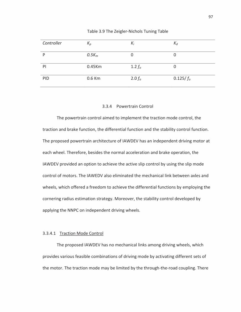
97
Table 3.9 The Zeigler-Nichols Tuning Table
Controller Kp Ki Kd
P 0.5Km 0 0
PI 0.45Km 1.2 fo 0
PID 0.6 Km 2.0 fo 0.125/ fo
3.3.4 Powertrain Control
The powertrain control aimed to implement the traction mode control, the
traction and brake function, the differential function and the stability control function.
The proposed powertrain architecture of IAWDEV has an independent driving motor at
each wheel. Therefore, besides the normal acceleration and brake operation, the
IAWDEV provided an option to achieve the active slip control by using the slip mode
control of motors. The IAWEDV also eliminated the mechanical link between axles and
wheels, which offered a freedom to achieve the differential functions by employing the
cornering radius estimation strategy. Moreover, the stability control developed by
applying the NNPC on independent driving wheels.
3.3.4.1 Traction Mode Control
The proposed IAWDEV has no mechanical links among driving wheels, which
provides various feasible combinations of driving mode by activating different sets of
the motor. The traction mode may be limited by the through-the-road coupling. There
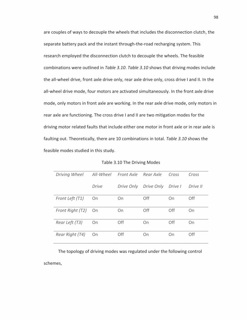
98
are couples of ways to decouple the wheels that includes the disconnection clutch, the
separate battery pack and the instant through-the-road recharging system. This
research employed the disconnection clutch to decouple the wheels. The feasible
combinations were outlined in Table 3.10. Table 3.10 shows that driving modes include
the all-wheel drive, front axle drive only, rear axle drive only, cross drive I and II. In the
all-wheel drive mode, four motors are activated simultaneously. In the front axle drive
mode, only motors in front axle are working. In the rear axle drive mode, only motors in
rear axle are functioning. The cross drive I and II are two mitigation modes for the
driving motor related faults that include either one motor in front axle or in rear axle is
faulting out. Theoretically, there are 10 combinations in total. Table 3.10 shows the
feasible modes studied in this study.
Table 3.10 The Driving Modes
Driving Wheel All-Wheel
Drive
Front Axle
Drive Only
Rear Axle
Drive Only
Cross
Drive I
Cross
Drive II
Front Left (T1) On On Off On Off
Front Right (T2) On On Off Off On
Rear Left (T3) On Off On Off On
Rear Right (T4) On Off On On Off
The topology of driving modes was regulated under the following control
schemes,
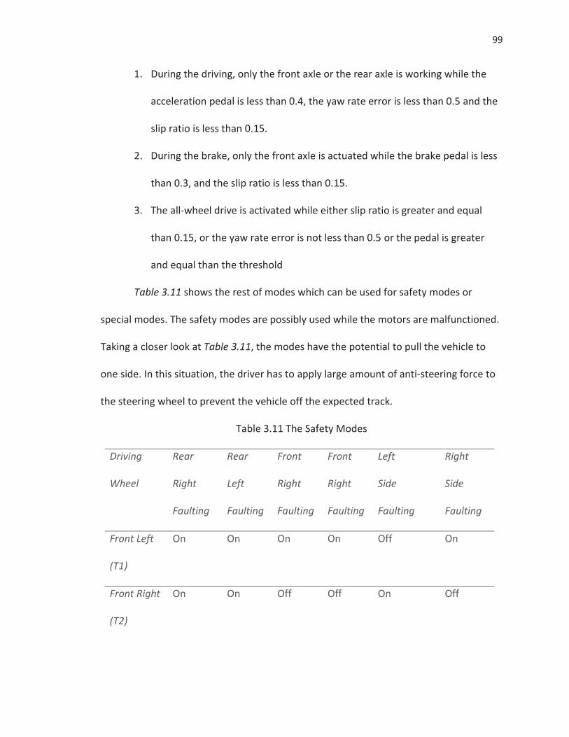
99
1. During the driving, only the front axle or the rear axle is working while the
acceleration pedal is less than 0.4, the yaw rate error is less than 0.5 and the
slip ratio is less than 0.15.
2. During the brake, only the front axle is actuated while the brake pedal is less
than 0.3, and the slip ratio is less than 0.15.
3. The all-wheel drive is activated while either slip ratio is greater and equal
than 0.15, or the yaw rate error is not less than 0.5 or the pedal is greater
and equal than the threshold
Table 3.11 shows the rest of modes which can be used for safety modes or
special modes. The safety modes are possibly used while the motors are malfunctioned.
Taking a closer look at Table 3.11, the modes have the potential to pull the vehicle to
one side. In this situation, the driver has to apply large amount of anti-steering force to
the steering wheel to prevent the vehicle off the expected track.
Table 3.11 The Safety Modes
Driving
Wheel
Rear
Right
Faulting
Rear
Left
Faulting
Front
Right
Faulting
Front
Right
Faulting
Left
Side
Faulting
Right
Side
Faulting
Front Left
(T1)
On On On On Off On
Front Right
(T2)
On On Off Off On Off
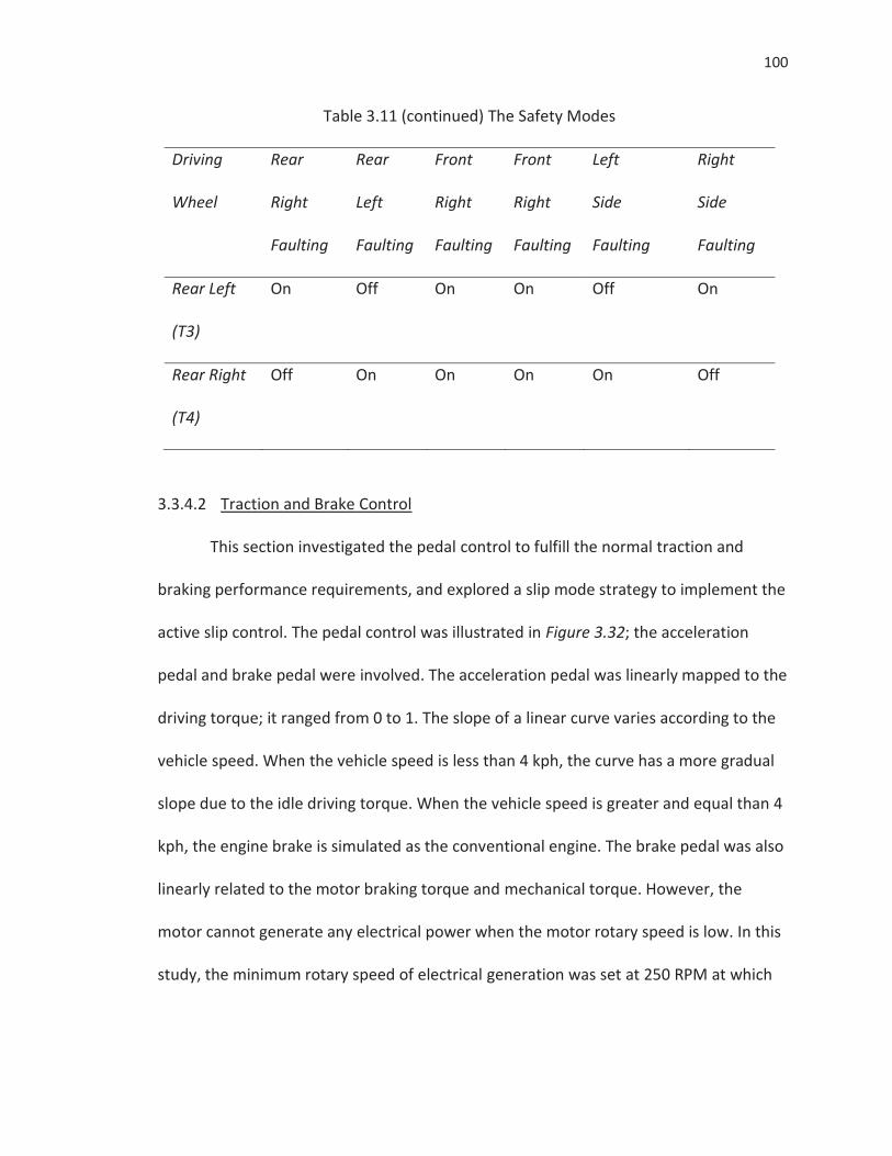
100
Table 3.11 (continued) The Safety Modes
Driving
Wheel
Rear
Right
Faulting
Rear
Left
Faulting
Front
Right
Faulting
Front
Right
Faulting
Left
Side
Faulting
Right
Side
Faulting
Rear Left
(T3)
On Off On On Off On
Rear Right
(T4)
Off On On On On Off
3.3.4.2 Traction and Brake Control
This section investigated the pedal control to fulfill the normal traction and
braking performance requirements, and explored a slip mode strategy to implement the
active slip control. The pedal control was illustrated in Figure 3.32; the acceleration
pedal and brake pedal were involved. The acceleration pedal was linearly mapped to the
driving torque; it ranged from 0 to 1. The slope of a linear curve varies according to the
vehicle speed. When the vehicle speed is less than 4 kph, the curve has a more gradual
slope due to the idle driving torque. When the vehicle speed is greater and equal than 4
kph, the engine brake is simulated as the conventional engine. The brake pedal was also
linearly related to the motor braking torque and mechanical torque. However, the
motor cannot generate any electrical power when the motor rotary speed is low. In this
study, the minimum rotary speed of electrical generation was set at 250 RPM at which
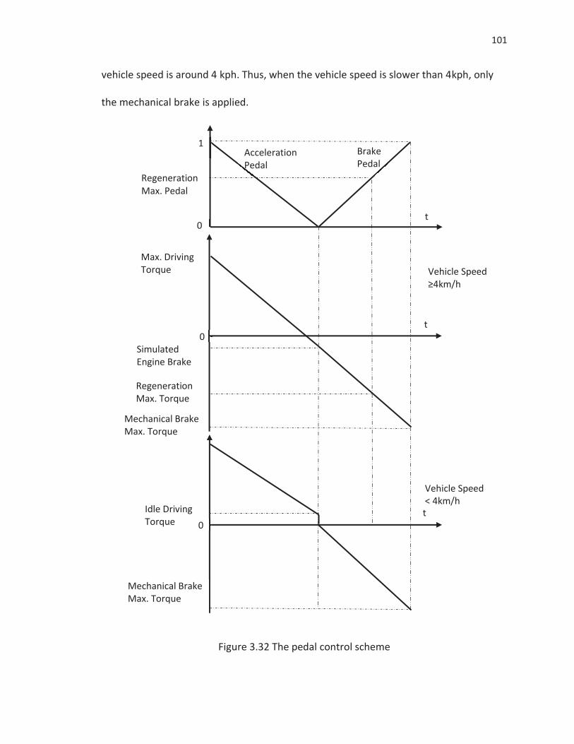
101
vehicle speed is around 4 kph. Thus, when the vehicle speed is slower than 4kph, only
the mechanical brake is applied.
Figure 3.32 The pedal control scheme
Regeneration Max. Pedal
1
0
0
0
Simulated Engine Brake
Max. Driving Torque
Mechanical Brake Max. Torque
Regeneration Max. Torque
Mechanical Brake Max. Torque
0
Idle Driving Torque
Acceleration Pedal
Brake Pedal
Vehicle Speed ≥4km/h
Vehicle Speed < 4km/h
t
t
t
102
Nassi and Sheiderman (1973) came up with a novel flow chart that uses the
rectangular box instead of the arrow chart to represent the algorithm; the box chart is
named as an N-S flow chart. This research employed the standardized N-S chart to
illustrate the entry and exit conditions for the traction and regeneration control body.
Figure 3.33 shows that the slip control function is triggered by a function switch at the
highest level; the slip function block is enabled while the switch is on. In further, the
controller enters the corresponding function branches on the basis of the wheel slip
ratio and pedal position.
According to the research conducted by Zanten, Erhardt and Lutz (1990), the
optimal values of wheel slip are between 0.08 and 0.3. This research used the
magnitude of slip ratio, 0.15, as the slip control entry threshold, and employed the slip
ratio, 0.2, as the target slip ratio. The entry threshold was designed to filter out control
intervening under good road conditions. The target slip ratio was ensured by a hybrid
sliding mode controller (HSMC) that forces the slip ratio error onto the slide mode
surface and retaining on the surface.
The slip control consists of the traction control function and the regeneration
brake slip control function. If the acceleration pedal is greater and equal than the dead
zone threshold and the wheel slip ratio is greater and equal than 0.15, then the traction
control is applied. Otherwise, the regeneration brake slip control is active. Both control
functions employed the sliding mode control (SMC). It is noticed that the anti-brake
skidding of the mechanical brake system is activated if the brake demand is over the
regeneration brake capacity. The anti-brake skidding of the mechanical brake system is
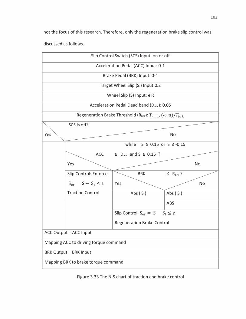
103
not the focus of this research. Therefore, only the regeneration brake slip control was
discussed as follows.
Slip Control Switch (SCS) Input: on or off
Acceleration Pedal (ACC) Input: 0-1
Brake Pedal (BRK) Input: 0-1
Target Wheel Slip (St) Input:0.2
Wheel Slip (S) Input: є R
Acceleration Pedal Dead band (Dacc): 0.05
Regeneration Brake Threshold (Rbrk):
Yes
SCS is off?
No
while S ≥ 0.15 or S ≤ -0.15
ACC
Yes
≥ Dacc and S ≥ 0.15 ?
No
Slip Control: Enforce
Traction Control
BRK
Yes
≤ Rbrk ?
No
Abs ( S ) Abs ( S )
ABS
Slip Control:
Regeneration Brake Control
ACC Output = ACC Input
Mapping ACC to driving torque command
BRK Output = BRK Input
Mapping BRK to brake torque command
Figure 3.33 The N-S chart of traction and brake control
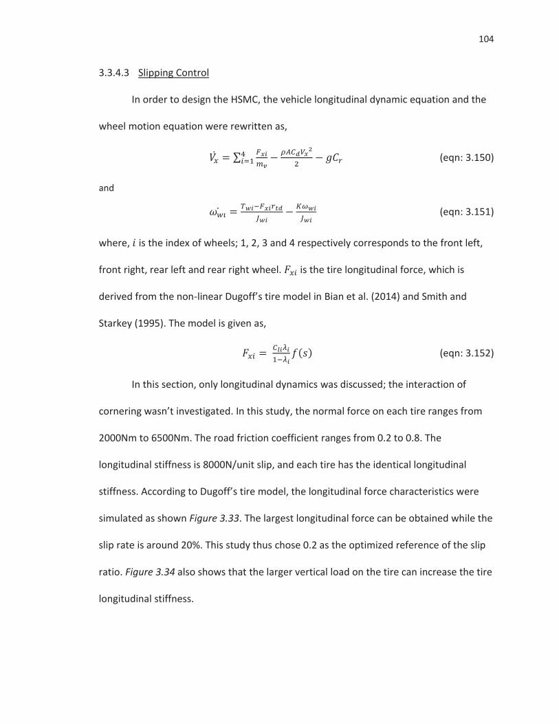
104
3.3.4.3 Slipping Control
In order to design the HSMC, the vehicle longitudinal dynamic equation and the
wheel motion equation were rewritten as,
(eqn: 3.150)
and
(eqn: 3.151)
where, is the index of wheels; 1, 2, 3 and 4 respectively corresponds to the front left,
front right, rear left and rear right wheel. is the tire longitudinal force, which is
derived from the non-linear Dugoff’s tire model in Bian et al. (2014) and Smith and
Starkey (1995). The model is given as,
(eqn: 3.152)
In this section, only longitudinal dynamics was discussed; the interaction of
cornering wasn’t investigated. In this study, the normal force on each tire ranges from
2000Nm to 6500Nm. The road friction coefficient ranges from 0.2 to 0.8. The
longitudinal stiffness is 8000N/unit slip, and each tire has the identical longitudinal
stiffness. According to Dugoff’s tire model, the longitudinal force characteristics were
simulated as shown Figure 3.33. The largest longitudinal force can be obtained while the
slip rate is around 20%. This study thus chose 0.2 as the optimized reference of the slip
ratio. Figure 3.34 also shows that the larger vertical load on the tire can increase the tire
longitudinal stiffness.
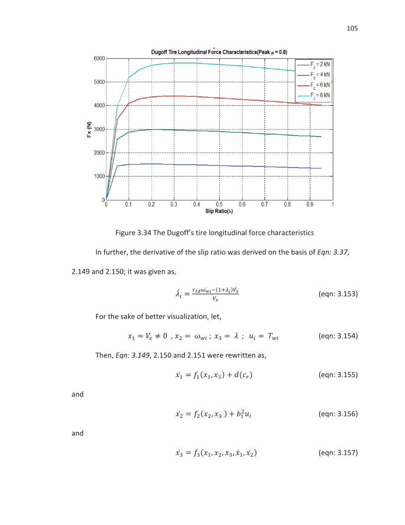
105
Figure 3.34 The Dugoff’s tire longitudinal force characteristics
In further, the derivative of the slip ratio was derived on the basis of Eqn: 3.37,
2.149 and 2.150; it was given as,
(eqn: 3.153)
For the sake of better visualization, let,
, (eqn: 3.154)
Then, Eqn: 3.149, 2.150 and 2.151 were rewritten as,
(eqn: 3.155)
and
(eqn: 3.156)
and
(eqn: 3.157)
106
and
(eqn: 3.158)
where, is the state vector; It should be noted that
are physically bounded; is the control scalar for ith wheel that is
bounded by driver command torque, and is 1 in this research; is the system
output.
Moreover, is the constant disturbance that is physically bounded by the
rolling resistance; it was represented as,
(eqn: 3.159)
The nonlinear dynamic of was derived from Eqn: 3.65,
(eqn: 3.160)
The nonlinear dynamics of was obtained as,
(eqn: 3.161)
The dynamics has nonlinear characteristic; it was derived as,
(eqn: 3.162)
By substituting Eqn: 3.152 and 2.153 into 2.154, Eqn: 3.154 was rewritten as
(eqn: 3.163)
where,
(eqn: 3.164)
The HSMC in this research was to enforce the slip ratio converges to the
reference value. Thus, the switch function was firstly designed as follows,
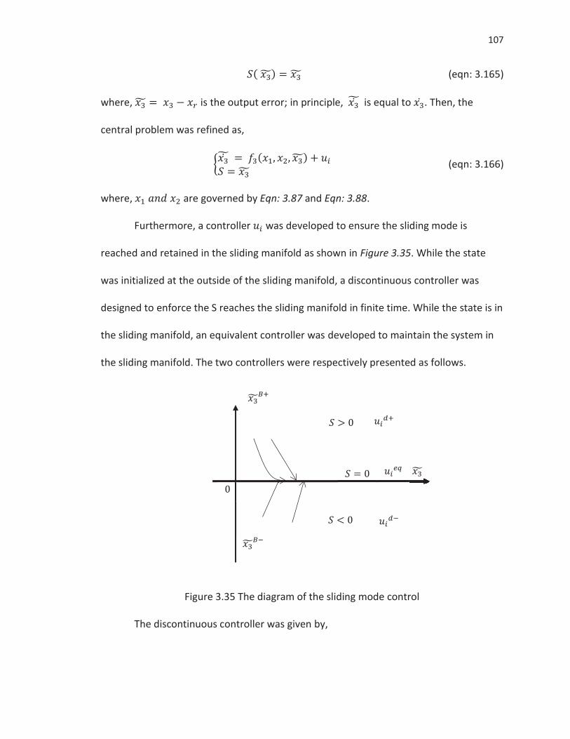
107
(eqn: 3.165)
where, is the output error; in principle, is equal to . Then, the
central problem was refined as,
(eqn: 3.166)
where, are governed by Eqn: 3.87 and Eqn: 3.88.
Furthermore, a controller was developed to ensure the sliding mode is
reached and retained in the sliding manifold as shown in Figure 3.35. While the state
was initialized at the outside of the sliding manifold, a discontinuous controller was
designed to enforce the S reaches the sliding manifold in finite time. While the state is in
the sliding manifold, an equivalent controller was developed to maintain the system in
the sliding manifold. The two controllers were respectively presented as follows.
Figure 3.35 The diagram of the sliding mode control
The discontinuous controller was given by,
108
(eqn: 3.167)
and,
(eqn: 3.168)
where, is the positive control gain; it was obtained by using the Lyapunov stability
theory. This study constructed the Lyapunov function of the following form,
(eqn: 3.169)
where, is positive definite; is zero only if S is zero. To ensure the trajectory of
converges to zero in finite time, the should satisfy the following properties,
for all (eqn: 3.170)
and
(eqn: 3.171)
Substitutes Eqn: 3.162 and 2.165 into Eqn: 3.168,
(eqn: 3.172)
As discussed above, is physically bounded. Eqn: 3.171 is satisfied as
long as,
(eqn: 3.173)
where, is a small positive number; it is close to zero. In order to achieve faster
convergence, should be larger.
Up to now, the discontinuous controller was designed; the gain was obtained
using Lyapunov stability theorem. It should be noted that is strict discontinuous,
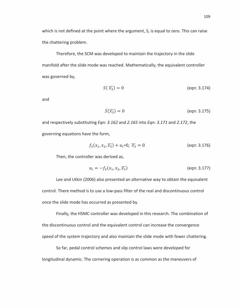
109
which is not defined at the point where the argument, S, is equal to zero. This can raise
the chattering problem.
Therefore, the SCM was developed to maintain the trajectory in the slide
manifold after the slide mode was reached. Mathematically, the equivalent controller
was governed by,
(eqn: 3.174)
and
(eqn: 3.175)
and respectively substituting Eqn: 3.162 and 2.165 into Eqn: 3.171 and 2.172, the
governing equations have the form,
=0, (eqn: 3.176)
Then, the controller was derived as,
(eqn: 3.177)
Lee and Utkin (2006) also presented an alternative way to obtain the equivalent
control. There method is to use a low-pass filter of the real and discontinuous control
once the slide mode has occurred as presented by.
Finally, the HSMC controller was developed in this research. The combination of
the discontinuous control and the equivalent control can increase the convergence
speed of the system trajectory and also maintain the slide mode with fewer chattering.
So far, pedal control schemes and slip control laws were developed for
longitudinal dynamic. The cornering operation is as common as the maneuvers of
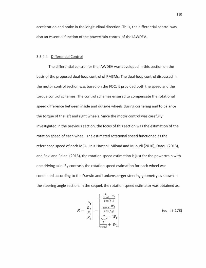
110
acceleration and brake in the longitudinal direction. Thus, the differential control was
also an essential function of the powertrain control of the IAWDEV.
3.3.4.4 Differential Control
The differential control for the IAWDEV was developed in this section on the
basis of the proposed dual-loop control of PMSMs. The dual-loop control discussed in
the motor control section was based on the FOC; it provided both the speed and the
torque control schemes. The control schemes ensured to compensate the rotational
speed difference between inside and outside wheels during cornering and to balance
the torque of the left and right wheels. Since the motor control was carefully
investigated in the previous section, the focus of this section was the estimation of the
rotation speed of each wheel. The estimated rotational speed functioned as the
referenced speed of each MCU. In K Hartani, Miloud and Miloudi (2010), Draou (2013),
and Ravi and Palani (2013), the rotation speed estimation is just for the powertrain with
one driving axle. By contrast, the rotation speed estimation for each wheel was
conducted according to the Darwin and Lankensperger steering geometry as shown in
the steering angle section. In the sequel, the rotation speed estimator was obtained as,
(eqn: 3.178)
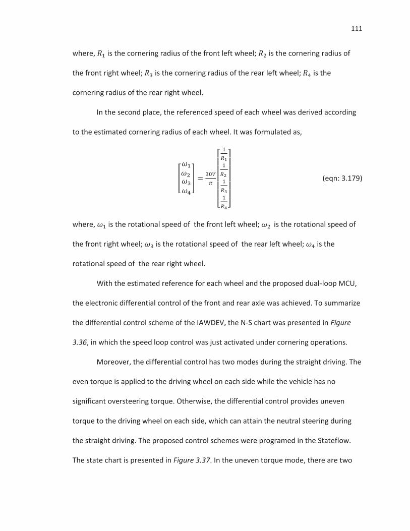
111
where, is the cornering radius of the front left wheel; is the cornering radius of
the front right wheel; is the cornering radius of the rear left wheel; is the
cornering radius of the rear right wheel.
In the second place, the referenced speed of each wheel was derived according
to the estimated cornering radius of each wheel. It was formulated as,
(eqn: 3.179)
where, is the rotational speed of the front left wheel; is the rotational speed of
the front right wheel; is the rotational speed of the rear left wheel; is the
rotational speed of the rear right wheel.
With the estimated reference for each wheel and the proposed dual-loop MCU,
the electronic differential control of the front and rear axle was achieved. To summarize
the differential control scheme of the IAWDEV, the N-S chart was presented in Figure
3.36, in which the speed loop control was just activated under cornering operations.
Moreover, the differential control has two modes during the straight driving. The
even torque is applied to the driving wheel on each side while the vehicle has no
significant oversteering torque. Otherwise, the differential control provides uneven
torque to the driving wheel on each side, which can attain the neutral steering during
the straight driving. The proposed control schemes were programed in the Stateflow.
The state chart is presented in Figure 3.37. In the uneven torque mode, there are two
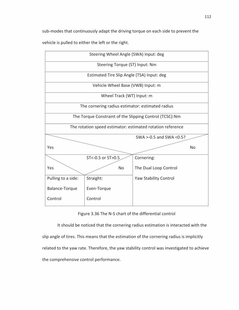
112
sub-modes that continuously adapt the driving torque on each side to prevent the
vehicle is pulled to either the left or the right.
Steering Wheel Angle (SWA) Input: deg
Steering Torque (ST) Input: Nm
Estimated Tire Slip Angle (TSA) Input: deg
Vehicle Wheel Base (VWB) Input: m
Wheel Track (WT) Input: m
The cornering radius estimator: estimated radius
The Torque Constraint of the Slipping Control (TCSC):Nm
The rotation speed estimator: estimated rotation reference
Yes
SWA >-0.5 and SWA <0.5?
No
Yes
ST<-0.5 or ST>0.5
No
Cornering:
The Dual Loop Control
Pulling to a side:
Balance-Torque
Control
Straight:
Even-Torque
Control
Yaw Stability Control
Figure 3.36 The N-S chart of the differential control
It should be noticed that the cornering radius estimation is interacted with the
slip angle of tires. This means that the estimation of the cornering radius is implicitly
related to the yaw rate. Therefore, the yaw stability control was investigated to achieve
the comprehensive control performance.
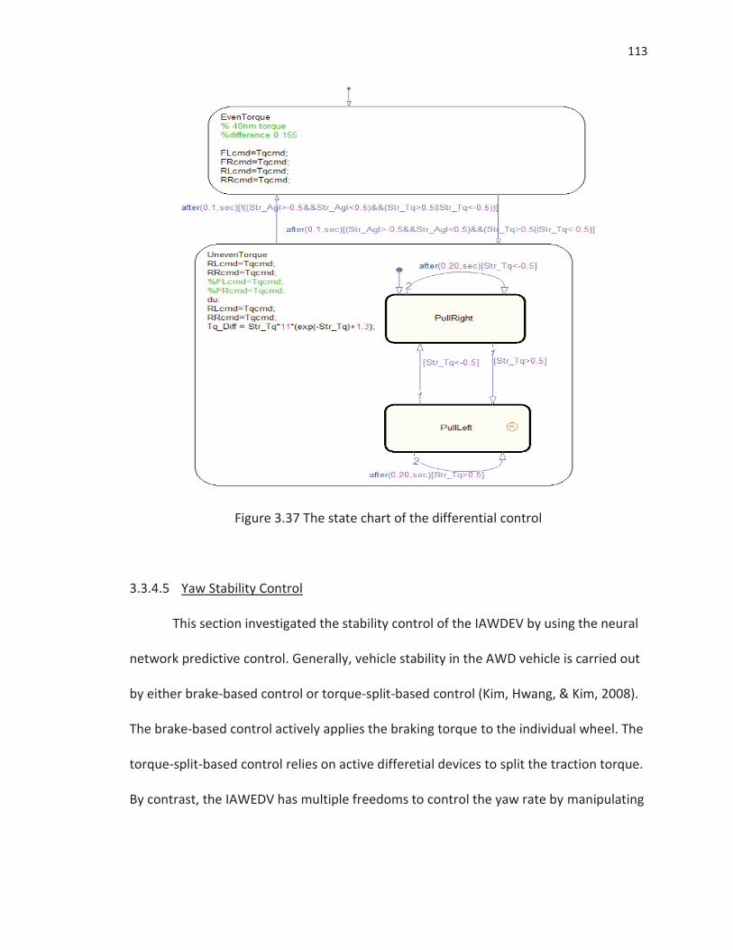
113
Figure 3.37 The state chart of the differential control
3.3.4.5 Yaw Stability Control
This section investigated the stability control of the IAWDEV by using the neural
network predictive control. Generally, vehicle stability in the AWD vehicle is carried out
by either brake-based control or torque-split-based control (Kim, Hwang, & Kim, 2008).
The brake-based control actively applies the braking torque to the individual wheel. The
torque-split-based control relies on active differetial devices to split the traction torque.
By contrast, the IAWEDV has multiple freedoms to control the yaw rate by manipulating
114
the torque on each independent driving wheel. In order to achieve the accurate yaw
stability control, the reference yaw rate should be estimated in the first place. With
some changes of the equations in the Bosh Automotive Handbook (2004), the reference
of yaw rate was estimated as,
(eqn: 3.180)
and
(eqn: 3.181)
Secondly, the proper torque reference should be assigned to each MCU; the
torque reference should be computed under the constraint of the yaw rate error, the
vehicle speed, the energy consumption and the tire slip rate. In principle, the control
problem is thus ended up with a complex torque topology problem; the possible
combination of torque control is up to 81. This study employed the neural network
method to manipulate the complex torque topology. Haykin (1999) stated that the
parallel processing capabilities of the neural network make it suitable for solving
complex and intractable problem. It should be noticed that the yaw dynamic is
inherently nonlinear due to the nonlinear characteristic of actual steering angle for each
wheel. In addition, the trigonometric function in Eqn: 3.10 also introduced the nonlinear
characteristic into the system. In this situation, the traditional control schemes for the
LTI system are not suitable anymore. Li et al. (2009) investigated an active yaw moment
control law using fuzzy logic. Anwar (2005) explored a generalized predictive control
method for the vehicle yaw stability control system. The researchers usually just focused
115
on the stability control for two-wheel drive, and didn’t involve the torque topology
problem for the AWD vehicle. This research developed a stability control by employing
the NNPC to establish the torque topology under multiple system constraints. Then, the
control framework was summarized in Figure 3.38, in which the NNPC consists of the
estimation model of yaw rate reference, the optimal controller and the neural network
predictive model (NNPM).
The optimal controller is strongly based on the predicted plant response over a
defined time horizon. The predictions were obtained by using the NNPM. The optimal
controller used the predictions to minimize the overall performance criterion as follows,
(eqn: 3.182)
where
(eqn: 3.183)
and
(eqn: 3.184)
where, k is the index of discrete time step; is the control
command vector in the specific horizon; in fact, the control vector is the torque
reference vector for each wheel; is the cost horizon and is 5 in this research; is the
weight factor and is 0.03 in this study; is the control horizon and 2 in this research.
The first term in the overall performance is to minimize the error between the
actual yaw response and the yaw reference. It should also be noticed that the significant
control transition can cost extra energy consumption and other disturbances to system
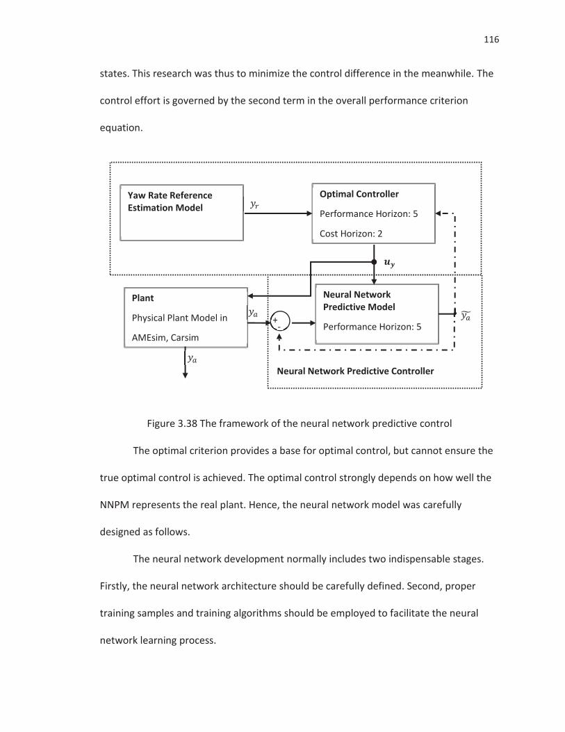
116
states. This research was thus to minimize the control difference in the meanwhile. The
control effort is governed by the second term in the overall performance criterion
equation.
Figure 3.38 The framework of the neural network predictive control
The optimal criterion provides a base for optimal control, but cannot ensure the
true optimal control is achieved. The optimal control strongly depends on how well the
NNPM represents the real plant. Hence, the neural network model was carefully
designed as follows.
The neural network development normally includes two indispensable stages.
Firstly, the neural network architecture should be carefully defined. Second, proper
training samples and training algorithms should be employed to facilitate the neural
network learning process.
Optimal Controller
Performance Horizon: 5
Cost Horizon: 2
Neural Network Predictive Model
Performance Horizon: 5
Yaw Rate Reference Estimation Model
Plant
Physical Plant Model in
AMEsim, Carsim
+ +-
Neural Network Predictive Controller
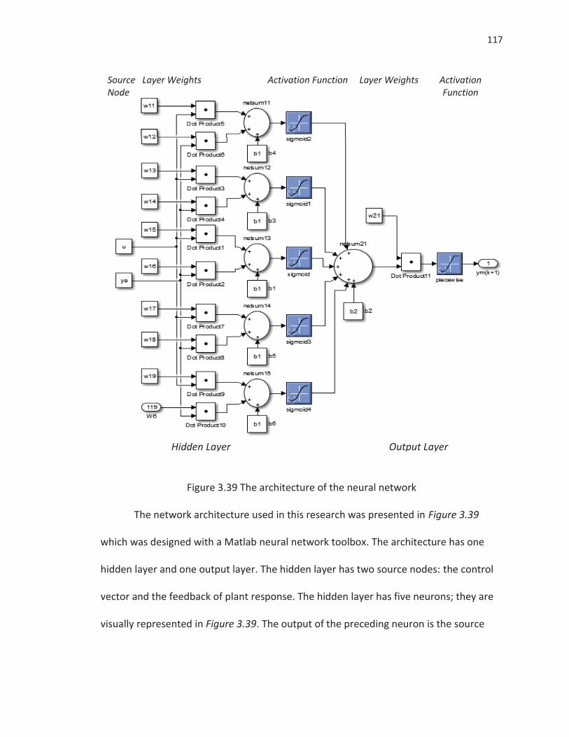
117
Figure 3.39 The architecture of the neural network
The network architecture used in this research was presented in Figure 3.39
which was designed with a Matlab neural network toolbox. The architecture has one
hidden layer and one output layer. The hidden layer has two source nodes: the control
vector and the feedback of plant response. The hidden layer has five neurons; they are
visually represented in Figure 3.39. The output of the preceding neuron is the source
Source Layer Weights Activation Function Layer Weights Activation Node Function
Hidden Layer Output Layer
118
node of the neuron in the output layer. The source node for the hidden layer consists of
the control vector and the actual response of the plant. In fact, the proposed
architecture is a multiple-layer structure which specifically has two layers. Cybenko
(1989) proved the theorem of Cybenko that a multi-layer perceptron can represent a
universal function approximator. This means the proposed architecture is able to
represent the mentioned non-linear yaw dynamic.
The neural network design mainly includes the design of the neuron, the
activation function and the layer. The neuron design was introduced in the first. The
input and output pair of neurons in the hidden layer was mathematically written as,
(eqn: 3.185)
and
(eqn: 3.186)
where,
(eqn: 3.187)
and
; (eqn: 3.188)
where, and respectively represents synaptic weights matrix and vector; is
the set of input neurons in the first layer; is the input vector of neuron is the
scalar of the plant response; is the bias vector of neurons in the
119
hidden layer; the bias actually applies an affine transformation to the linear combiner of
the output ; is the activation function; is the
output vector of neurons.
By using the similar approach, the input and output pair of neurons in the output
layer was derived as,
(eqn: 3.189)
and
(eqn: 3.190)
where, = [ ] is the weight vector of output neurons;
is the prediction output scalar of the neuron model; is the bias of the out neuron;
is the activation function.
The activation function has three types: the threshold function, the piecewise
linear function and the sigmoid function. In this study, the sigmoid function was
employed for the hidden layer; the piecewise linear function was used for the output
layer. Let , and then the activation functions were respectively given as,
(eqn: 3.191)
and
(eqn: 3.192)
So far, the complete neural network architecture was discussed. In the sequel,
the learning mode and learning algorithm was investigated.
120
The learning modes include the offline mode and the online mode. As defined by
Kriesel (2007), the offline learning mode is also called batch learning mode in which the
weights are adjusted all at once; the online learning learns directly from the errors of
each training sample. It needs to mention that the offline learning is based on well-
prepared samples of each pattern; the online learning relies on the instantaneous
training sample either from the high fidelity model simulation or from the physical plant
testing. This research proposed a model-based hybrid learning mode (MHLM) in which
the learning process is parallel with the model simulation run; it periodically conducts
batch learning while 300 simulation samples have been accumulated in the memory.
This research developed the customized yaw dynamic model according to the equations.
The model was built in AMEsim R12 and simulated by using co-simulation technology.
The purpose of learning process is to find the suitable set of synaptic weights
that can minimize the error between the predicted response and the actual response. In
other words, this research must investigate how to adjust the synaptic weights to
minimize the modeling error. In order to achieve this objective, this study employed the
back propagation algorithm. Before the further investigation of the algorithm, this
research defined the prediction error as the function of all synaptic weights. It is given
as,
(eqn: 3.193)
where, is the entire weights set, and mapped to the dimensional error space; is
the number of teaching patterns.
121
To further simplify the derivation, the pattern is fixed at the t-th pattern for
instance. The error function is becoming an arbitrary but finite-dimensional function,
(eqn: 3.194)
and then,
(eqn: 3.195)
where, is the teaching sample space, a finite dimensional real space. In an analogy to
the Euclidean distance, the error function was specifically defined as,
(eqn: 3.196)
In addition, this research defined the one step adjustment of the weights for the
-th sample vector as follows. The definition is based on Hebb’s postulate of learning
rule in Hebb (1949) and the mathematical form of Hebbian learning in Haykin (1999). It
was given as,
(eqn: 3.197)
and applying the chain rule of derivative, so Eqn: 3.196 is factored as,
(eqn: 3.198)
then, expanding each vector in Eqn: 3.197, and also extending the teaching sample
vector to the entire teaching sample space, the generalized and programmable back
propagation algorithm was derived as,
(eqn: 3.199)
where,
122
(eqn: 3.200)
and , a positive constant, is the learning rate; the larger learning rate can enhance the
learning speed but could skip the minima. In order to mitigate the skipping issue, the
learning rate can be as a linear proportional function of the error (Kriesel, 2007). The
linear proportional learning rate can achieve faster learning at large error and more
accurate learning at small error. However, the linear proportional learning function is
easier to introduce the Zeno oscillation issue. This research thus proposed an
exponential-based learning function. The proposed function has the similar advantage
of the linear proportional learning function, but can significantly reduce the oscillation.
It was given as,
(eqn: 3.201)
where, is the gain of learning rate function and is 1 while the error is over ;
otherwise, is zero. It should be noticed that the learning process should be stopped
as soon as is smaller than the learning tolerance, 0.0001 in this research.
To summarize, this research designed a NNPC to optimize the yaw dynamic and
control energy. The NNPM employed a two-layer architecture which was taught in
hybrid learning mode and back propagation learning algorithm. The complete stability
controller was finally verified by employing the double change procedure. So far, the
proposed MCU and PCU were completed. In order to follow the V-cycle process, the
verification of controllers was also involved in this research.
123
3.4 Verification Method
This section started by introducing a popular process of the model-based
development and verification. The process is often called as a V-cycle. The V-cycle
graphically illustrates the development process and the interaction between individual
development stages. With some alterations to the V-cycle in Toman, Kerlin and Singule
(2011), Figure 3.40 shows that the V-cycle mainly consists of development stages and
validation stages. The development stages are on the left side of V cycle; they include
the system definition and requirement, the high level function (HLF) design and the
component level design. The validation stages are on the right side; they cover the unit
test and verification, the function test and verification, and the system validation. The
break point is the target code generation; the code generation technology has large
varieties, such as xPC, AutoSar and Power PC.
This research designed the high level controller, PCU, and the component level
controller, MCU, in above sections. This section focused on the validation of controllers
by using the technology of MIL, SIL and HIL.
According to the available resources, this research adapted the presented V-
cycle to the unique challenges in this research. Due to the limitation of the funding and
facilities, the vehicle prototype wasn’t built; the test on the proving ground wasn’t
feasible. In order to delimit these limitations, the MIL and SIL were employed for the
MCU verification. Figure 3.41 illustrated these two verification methods of the MCU.
MIL is a virtual and ideal simulation; the interface in the model may not exist in the
physical world. Even though MIL is not a real-time simulation and limited by memory
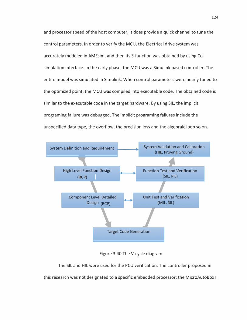
124
and processor speed of the host computer, it does provide a quick channel to tune the
control parameters. In order to verify the MCU, the Electrical drive system was
accurately modeled in AMEsim, and then its S-function was obtained by using Co-
simulation interface. In the early phase, the MCU was a Simulink based controller. The
entire model was simulated in Simulink. When control parameters were nearly tuned to
the optimized point, the MCU was compiled into executable code. The obtained code is
similar to the executable code in the target hardware. By using SIL, the implicit
programing failure was debugged. The implicit programing failures include the
unspecified data type, the overflow, the precision loss and the algebraic loop so on.
Figure 3.40 The V-cycle diagram
The SIL and HIL were used for the PCU verification. The controller proposed in
this research was not designated to a specific embedded processor; the MicroAutoBox II
System Definition and Requirement
High Level Function Design
Component Level Detailed Design
Target Code Generation
Unit Test and Verification (MIL, SIL)
Function Test and Verification (SIL, PIL)
System Validation and Calibration (HIL, Proving Ground)
(RCP)
n (RCP)
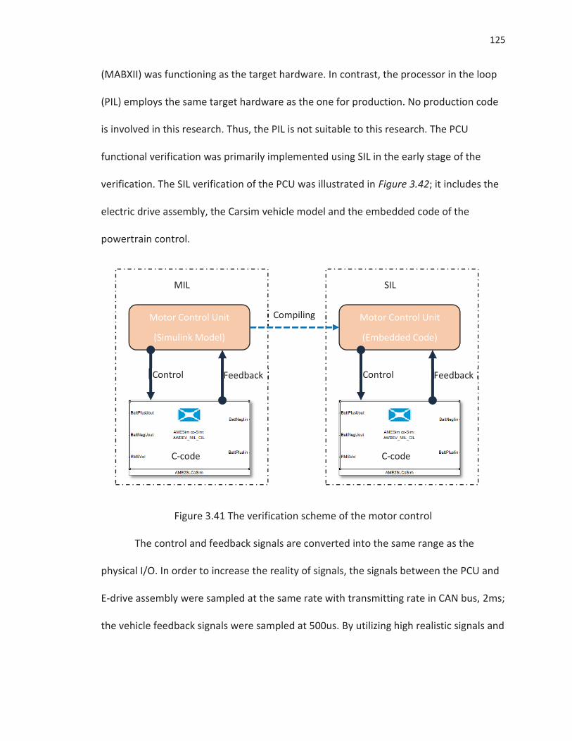
125
(MABXII) was functioning as the target hardware. In contrast, the processor in the loop
(PIL) employs the same target hardware as the one for production. No production code
is involved in this research. Thus, the PIL is not suitable to this research. The PCU
functional verification was primarily implemented using SIL in the early stage of the
verification. The SIL verification of the PCU was illustrated in Figure 3.42; it includes the
electric drive assembly, the Carsim vehicle model and the embedded code of the
powertrain control.
Figure 3.41 The verification scheme of the motor control
The control and feedback signals are converted into the same range as the
physical I/O. In order to increase the reality of signals, the signals between the PCU and
E-drive assembly were sampled at the same rate with transmitting rate in CAN bus, 2ms;
the vehicle feedback signals were sampled at 500us. By utilizing high realistic signals and
Motor Control Unit
(Simulink Model)
MIL
Control Feedback
C-code
Motor Control Unit
(Embedded Code)
SIL
Control Feedback
C-code
Compiling
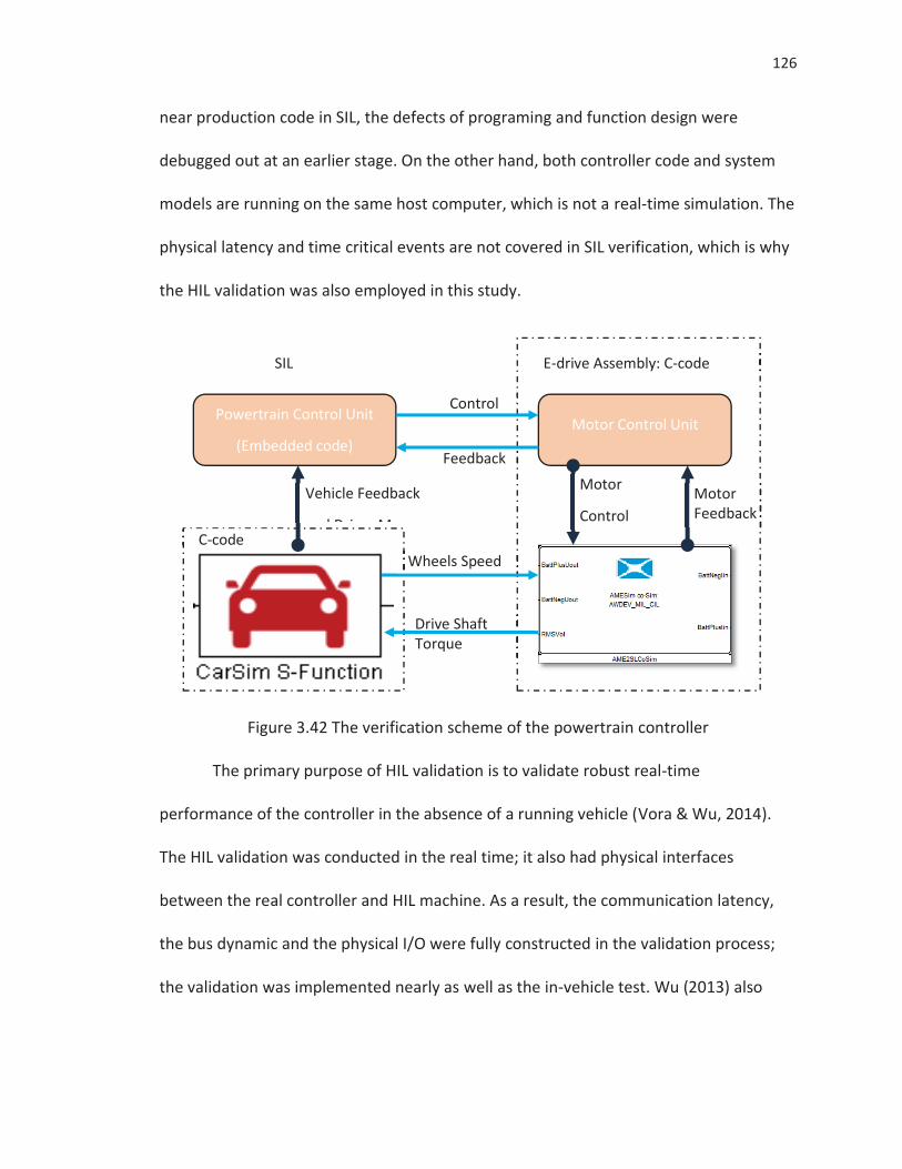
126
near production code in SIL, the defects of programing and function design were
debugged out at an earlier stage. On the other hand, both controller code and system
models are running on the same host computer, which is not a real-time simulation. The
physical latency and time critical events are not covered in SIL verification, which is why
the HIL validation was also employed in this study.
Figure 3.42 The verification scheme of the powertrain controller
The primary purpose of HIL validation is to validate robust real-time
performance of the controller in the absence of a running vehicle (Vora & Wu, 2014).
The HIL validation was conducted in the real time; it also had physical interfaces
between the real controller and HIL machine. As a result, the communication latency,
the bus dynamic and the physical I/O were fully constructed in the validation process;
the validation was implemented nearly as well as the in-vehicle test. Wu (2013) also
Powertrain Control Unit
(Embedded code)
SIL
Vehicle Feedback
and Driver Maneaur
Motor Control Unit
Motor
Control Motor Feedback
E-drive Assembly: C-code
C-code
Control
Feedback
Wheels Speed
Drive Shaft Torque
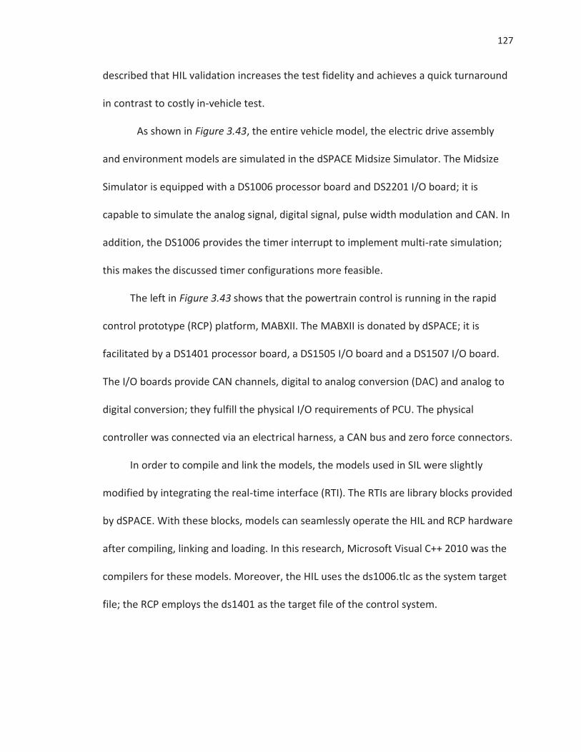
127
described that HIL validation increases the test fidelity and achieves a quick turnaround
in contrast to costly in-vehicle test.
As shown in Figure 3.43, the entire vehicle model, the electric drive assembly
and environment models are simulated in the dSPACE Midsize Simulator. The Midsize
Simulator is equipped with a DS1006 processor board and DS2201 I/O board; it is
capable to simulate the analog signal, digital signal, pulse width modulation and CAN. In
addition, the DS1006 provides the timer interrupt to implement multi-rate simulation;
this makes the discussed timer configurations more feasible.
The left in Figure 3.43 shows that the powertrain control is running in the rapid
control prototype (RCP) platform, MABXII. The MABXII is donated by dSPACE; it is
facilitated by a DS1401 processor board, a DS1505 I/O board and a DS1507 I/O board.
The I/O boards provide CAN channels, digital to analog conversion (DAC) and analog to
digital conversion; they fulfill the physical I/O requirements of PCU. The physical
controller was connected via an electrical harness, a CAN bus and zero force connectors.
In order to compile and link the models, the models used in SIL were slightly
modified by integrating the real-time interface (RTI). The RTIs are library blocks provided
by dSPACE. With these blocks, models can seamlessly operate the HIL and RCP hardware
after compiling, linking and loading. In this research, Microsoft Visual C++ 2010 was the
compilers for these models. Moreover, the HIL uses the ds1006.tlc as the system target
file; the RCP employs the ds1401 as the target file of the control system.
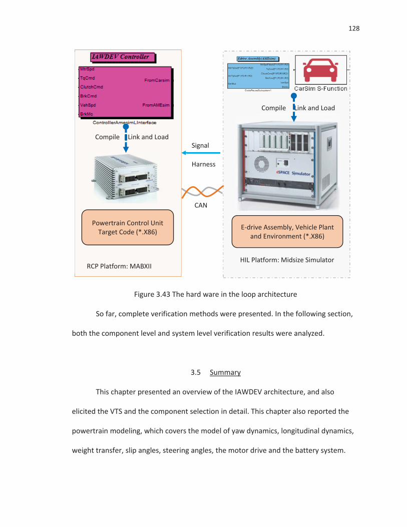
128
Figure 3.43 The hard ware in the loop architecture
So far, complete verification methods were presented. In the following section,
both the component level and system level verification results were analyzed.
3.5 Summary
This chapter presented an overview of the IAWDEV architecture, and also
elicited the VTS and the component selection in detail. This chapter also reported the
powertrain modeling, which covers the model of yaw dynamics, longitudinal dynamics,
weight transfer, slip angles, steering angles, the motor drive and the battery system.
Powertrain Control Unit Target Code (*.X86)
Compile Link and Load
RCP Platform: MABXII
E-drive Assembly, Vehicle Plant and Environment (*.X86)
Compile Link and Load
HIL Platform: Midsize Simulator
CAN
Signal
Harness
129
Sequentially, the insight of controller development was provided. The traction
and braking control, the slipping control, the differential control and the yaw stability
control were involved in the controller development. The sliding mode control and
neural network predictive control were carefully discussed. The mathematical proof
offered the evidence that the HSMC and NNPC are achievable and stable.
Finally, the verification method was introduced. The verification methods mainly
include the technologies of MIL, SIL and HIL.
130
CHAPTER 4. RESULTS AND DISCUSSION
As mentioned previously, the aim of this research was to propose the IAWDEV
powertrain and develop the corresponding controller at the component level and the
function level. This research was also attempted to eliminate the tire skidding and
enhance vehicle cornering stability, which wasn’t systematically solved by previous
researchers. Generally speaking, the overall design of the IAWDEV powertrain assembly
can fulfill the VTS requirements. The control schemes on the basis of proposed models
can achieve the anti-slip, differential and yaw stability controls in more stable and
efficient manner. The analysis of results is divided into two parts as follows: the IAWDEV
powertrain evaluation and control performance analysis.
4.1 IAWDEV Powertrain Evaluation
This section presented the comprehensive evaluation of the IAWDEV powertrain
architecture. The IAWDEV was modeled in the LMS AMESim R12 on the basis of the
models discussed in the section of vehicle powertrain modeling. The model was exactly
parameterized with selected component parameters. LMS AMESim is one of the most
creditable simulation platforms for multi-discipline system. The simulations were
conducted in a dynamic simulation mode and with the fixed time step solver. The
131
powertrain was controlled by the proposed traction mode, traction and brake controls.
To the author’s knowledge, it was found that the IAWDEV drivetrain had less
weight than TCAWDEV and dual-axle AWDEV, but had larger gross than the
conventional AWD due to the heavy battery system. Moreover, the powertrain fulfilled
the requirements in the predefined VTS, and achieved much better performance in
some aspects. This implicitly means that the components were correctly sized by using
presented estimation methods.
The battery OEMs and research institutions are investing tremendous resources
in battery systems. It should be noticed that the battery was not the focus of this
research. This research was conducted under the assumption that the battery
technology has been feasible and acceptable to function as the power unit of the vehicle.
The battery modeling discussed in this research was only aiming to develop and verify
control systems. Thus, this research that powertrain variants have the identical battery
system. Then, the weight of drivetrain components was compared carefully.
4.1.1 Weight Analysis
In order to accurately evaluate the powertrain design, this study firstly
conducted the analysis of drivetrain weight to finalize the curb weight of IAWDEV as
1634.3 kg. The weight analysis was focused on drivetrain components, such as the
motor, transfer case, differential, starter, alternator and shaft. The motor used in the
different powertrain has the same power. Then, the analysis was presented in Table 4.1.
The conventional AWD powertrain data were obtained from the Autonomie 2010. The
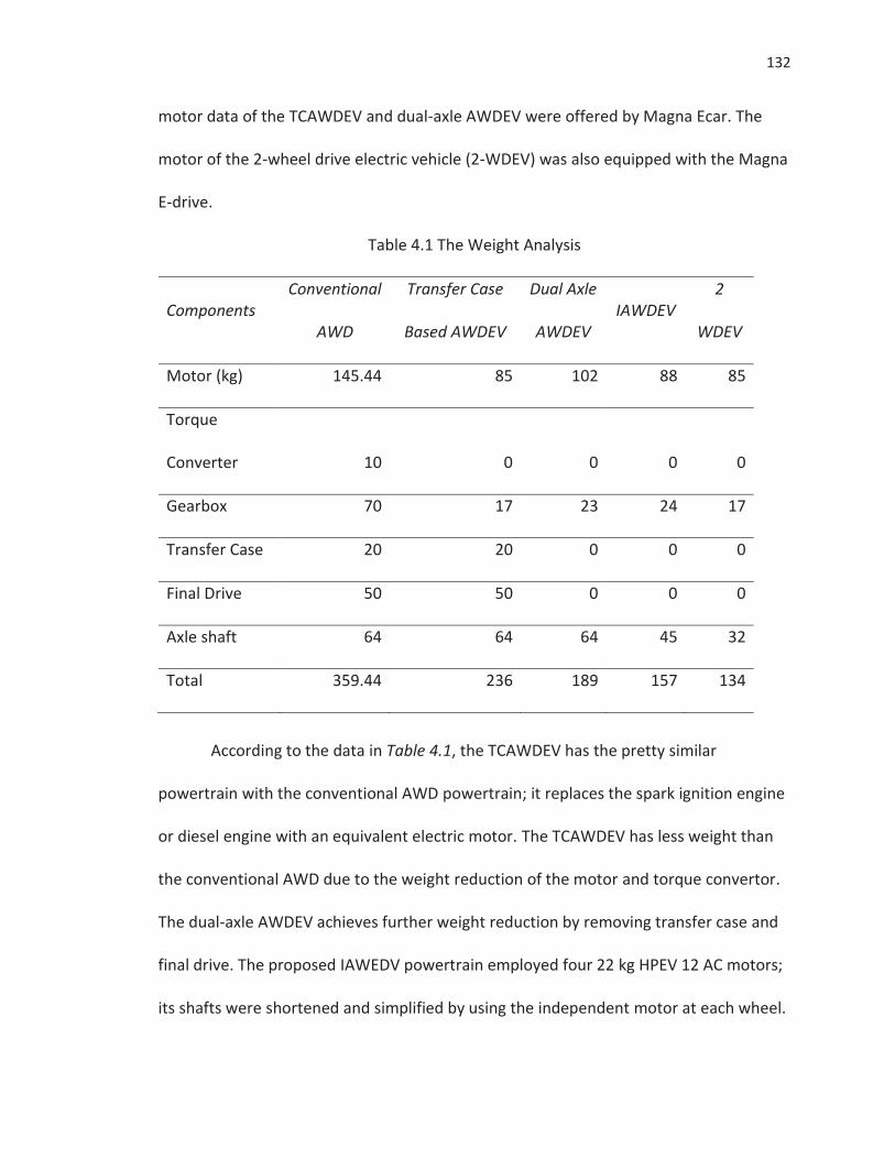
132
motor data of the TCAWDEV and dual-axle AWDEV were offered by Magna Ecar. The
motor of the 2-wheel drive electric vehicle (2-WDEV) was also equipped with the Magna
E-drive.
Table 4.1 The Weight Analysis
Components Conventional
AWD
Transfer Case
Based AWDEV
Dual Axle
AWDEV IAWDEV
2
WDEV
Motor (kg) 145.44 85 102 88 85
Torque
Converter 10 0 0 0 0
Gearbox 70 17 23 24 17
Transfer Case 20 20 0 0 0
Final Drive 50 50 0 0 0
Axle shaft 64 64 64 45 32
Total 359.44 236 189 157 134
According to the data in Table 4.1, the TCAWDEV has the pretty similar
powertrain with the conventional AWD powertrain; it replaces the spark ignition engine
or diesel engine with an equivalent electric motor. The TCAWDEV has less weight than
the conventional AWD due to the weight reduction of the motor and torque convertor.
The dual-axle AWDEV achieves further weight reduction by removing transfer case and
final drive. The proposed IAWEDV powertrain employed four 22 kg HPEV 12 AC motors;
its shafts were shortened and simplified by using the independent motor at each wheel.
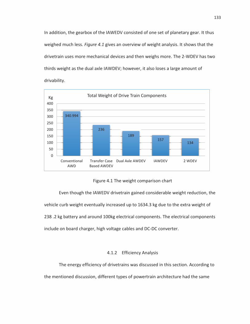
133
In addition, the gearbox of the IAWEDV consisted of one set of planetary gear. It thus
weighed much less. Figure 4.1 gives an overview of weight analysis. It shows that the
drivetrain uses more mechanical devices and then weighs more. The 2-WDEV has two
thirds weight as the dual axle IAWDEV; however, it also loses a large amount of
drivability.
Figure 4.1 The weight comparison chart
Even though the IAWEDV drivetrain gained considerable weight reduction, the
vehicle curb weight eventually increased up to 1634.3 kg due to the extra weight of
238 .2 kg battery and around 100kg electrical components. The electrical components
include on board charger, high voltage cables and DC-DC converter.
4.1.2 Efficiency Analysis
The energy efficiency of drivetrains was discussed in this section. According to
the mentioned discussion, different types of powertrain architecture had the same
340.994
236
189 157
134
0
50
100
150
200
250
300
350
400
ConventionalAWD
Transfer CaseBased AWDEV
Dual Axle AWDEV IAWDEV 2 WDEV
Total Weight of Drive Train Components Kg
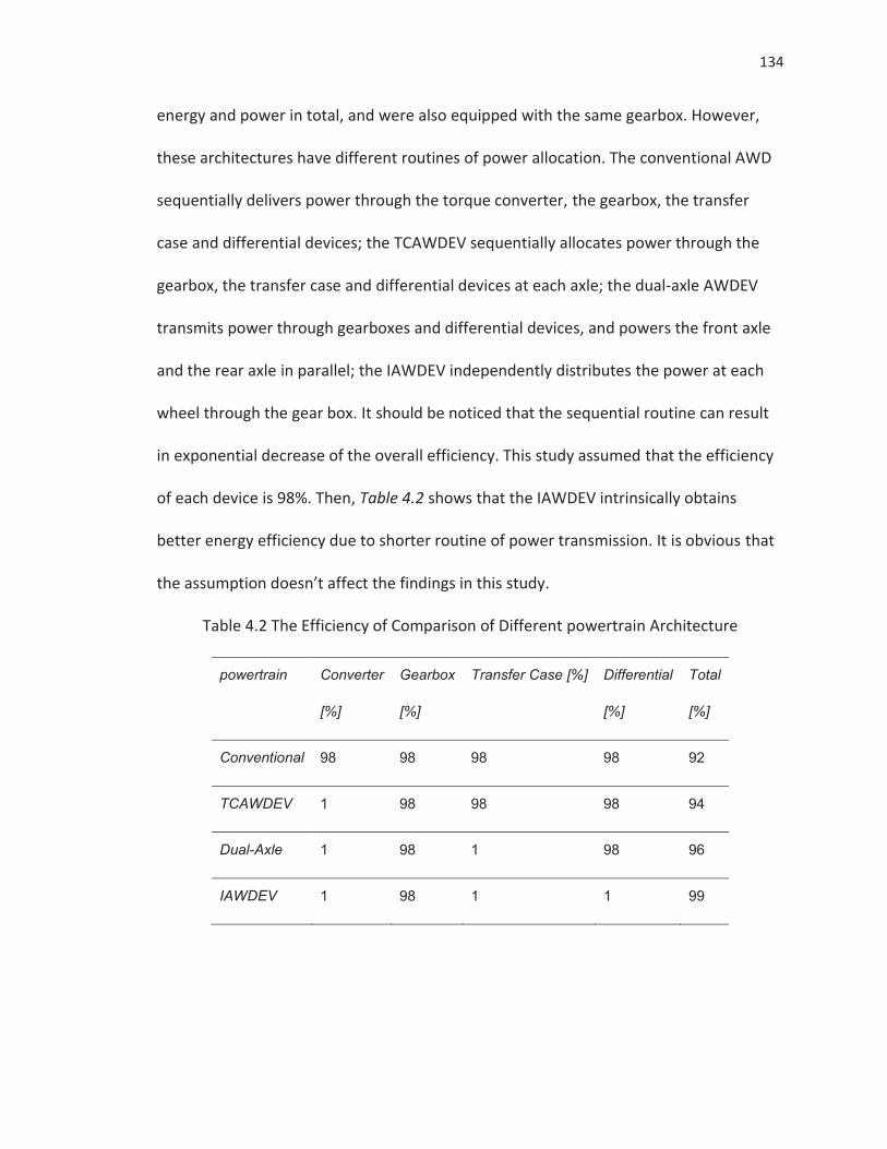
134
energy and power in total, and were also equipped with the same gearbox. However,
these architectures have different routines of power allocation. The conventional AWD
sequentially delivers power through the torque converter, the gearbox, the transfer
case and differential devices; the TCAWDEV sequentially allocates power through the
gearbox, the transfer case and differential devices at each axle; the dual-axle AWDEV
transmits power through gearboxes and differential devices, and powers the front axle
and the rear axle in parallel; the IAWDEV independently distributes the power at each
wheel through the gear box. It should be noticed that the sequential routine can result
in exponential decrease of the overall efficiency. This study assumed that the efficiency
of each device is 98%. Then, Table 4.2 shows that the IAWDEV intrinsically obtains
better energy efficiency due to shorter routine of power transmission. It is obvious that
the assumption doesn’t affect the findings in this study.
Table 4.2 The Efficiency of Comparison of Different powertrain Architecture
powertrain Converter
[%]
Gearbox
[%]
Transfer Case [%] Differential
[%]
Total
[%]
Conventional 98 98 98 98 92
TCAWDEV 1 98 98 98 94
Dual-Axle 1 98 1 98 96
IAWDEV 1 98 1 1 99
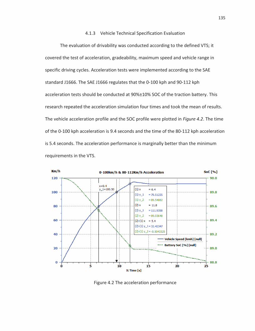
135
4.1.3 Vehicle Technical Specification Evaluation
The evaluation of drivability was conducted according to the defined VTS; it
covered the test of acceleration, gradeability, maximum speed and vehicle range in
specific driving cycles. Acceleration tests were implemented according to the SAE
standard J1666. The SAE J1666 regulates that the 0-100 kph and 90-112 kph
acceleration tests should be conducted at 90%±10% SOC of the traction battery. This
research repeated the acceleration simulation four times and took the mean of results.
The vehicle acceleration profile and the SOC profile were plotted in Figure 4.2. The time
of the 0-100 kph acceleration is 9.4 seconds and the time of the 80-112 kph acceleration
is 5.4 seconds. The acceleration performance is marginally better than the minimum
requirements in the VTS.
Figure 4.2 The acceleration performance
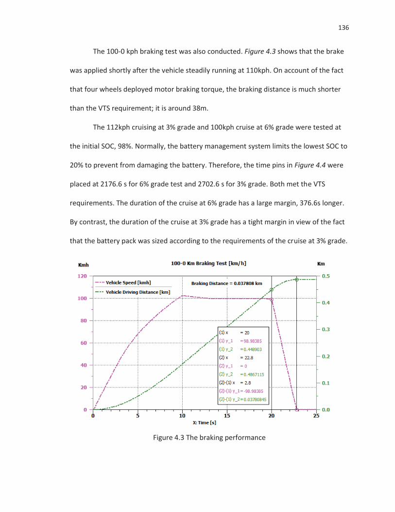
136
The 100-0 kph braking test was also conducted. Figure 4.3 shows that the brake
was applied shortly after the vehicle steadily running at 110kph. On account of the fact
that four wheels deployed motor braking torque, the braking distance is much shorter
than the VTS requirement; it is around 38m.
The 112kph cruising at 3% grade and 100kph cruise at 6% grade were tested at
the initial SOC, 98%. Normally, the battery management system limits the lowest SOC to
20% to prevent from damaging the battery. Therefore, the time pins in Figure 4.4 were
placed at 2176.6 s for 6% grade test and 2702.6 s for 3% grade. Both met the VTS
requirements. The duration of the cruise at 6% grade has a large margin, 376.6s longer.
By contrast, the duration of the cruise at 3% grade has a tight margin in view of the fact
that the battery pack was sized according to the requirements of the cruise at 3% grade.
Figure 4.3 The braking performance
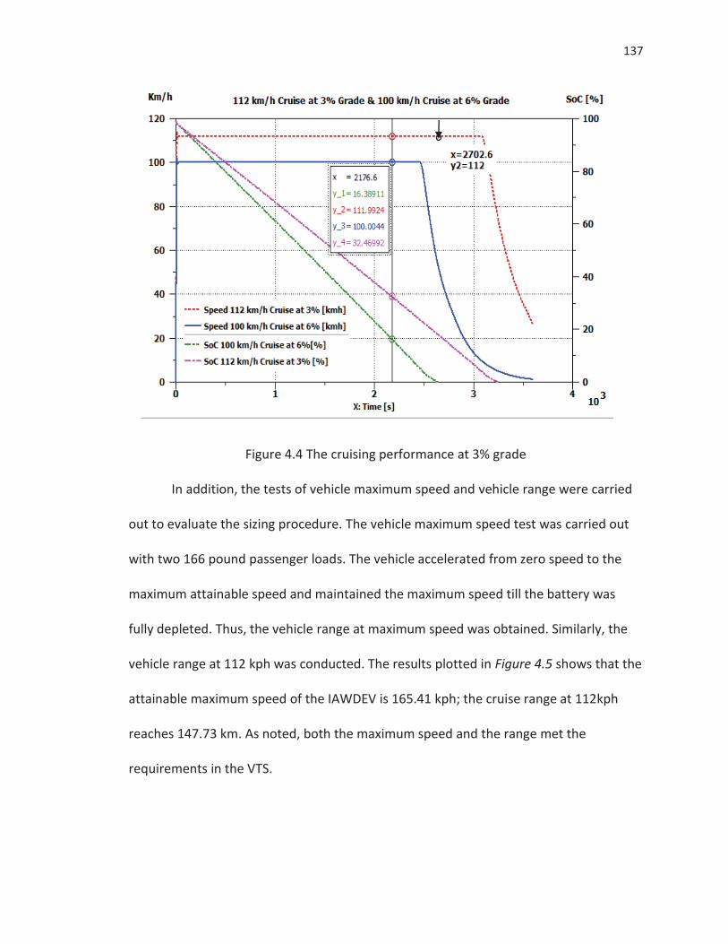
137
Figure 4.4 The cruising performance at 3% grade
In addition, the tests of vehicle maximum speed and vehicle range were carried
out to evaluate the sizing procedure. The vehicle maximum speed test was carried out
with two 166 pound passenger loads. The vehicle accelerated from zero speed to the
maximum attainable speed and maintained the maximum speed till the battery was
fully depleted. Thus, the vehicle range at maximum speed was obtained. Similarly, the
vehicle range at 112 kph was conducted. The results plotted in Figure 4.5 shows that the
attainable maximum speed of the IAWDEV is 165.41 kph; the cruise range at 112kph
reaches 147.73 km. As noted, both the maximum speed and the range met the
requirements in the VTS.
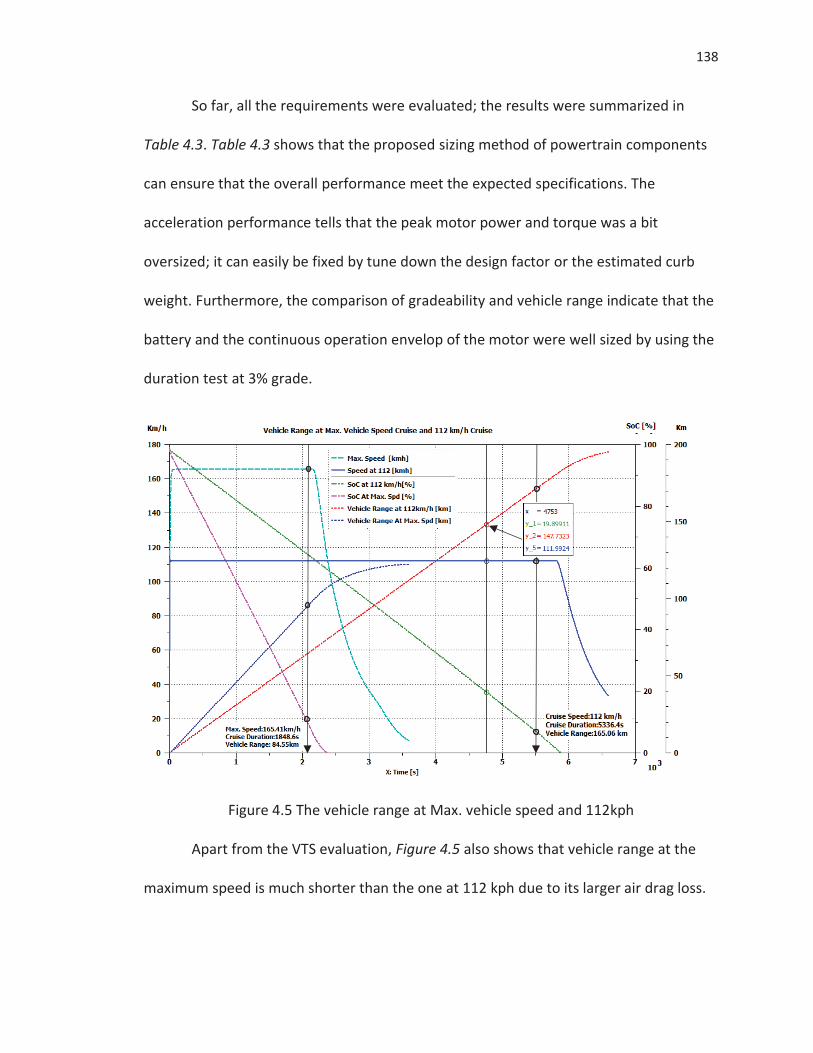
138
So far, all the requirements were evaluated; the results were summarized in
Table 4.3. Table 4.3 shows that the proposed sizing method of powertrain components
can ensure that the overall performance meet the expected specifications. The
acceleration performance tells that the peak motor power and torque was a bit
oversized; it can easily be fixed by tune down the design factor or the estimated curb
weight. Furthermore, the comparison of gradeability and vehicle range indicate that the
battery and the continuous operation envelop of the motor were well sized by using the
duration test at 3% grade.
Figure 4.5 The vehicle range at Max. vehicle speed and 112kph
Apart from the VTS evaluation, Figure 4.5 also shows that vehicle range at the
maximum speed is much shorter than the one at 112 kph due to its larger air drag loss.
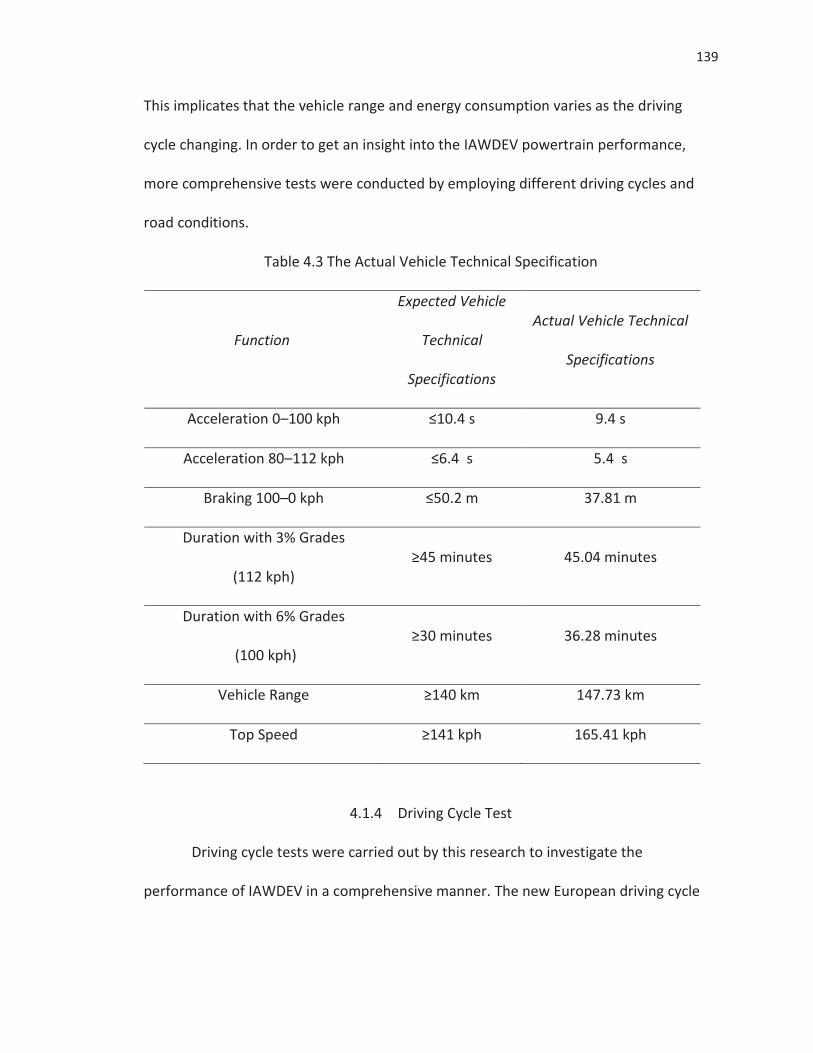
139
This implicates that the vehicle range and energy consumption varies as the driving
cycle changing. In order to get an insight into the IAWDEV powertrain performance,
more comprehensive tests were conducted by employing different driving cycles and
road conditions.
Table 4.3 The Actual Vehicle Technical Specification
Function
Expected Vehicle
Technical
Specifications
Actual Vehicle Technical
Specifications
Acceleration 0–100 kph ≤10.4 s 9.4 s
Acceleration 80–112 kph ≤6.4 s 5.4 s
Braking 100–0 kph ≤50.2 m 37.81 m
Duration with 3% Grades
(112 kph) ≥45 minutes 45.04 minutes
Duration with 6% Grades
(100 kph) ≥30 minutes 36.28 minutes
Vehicle Range ≥140 km 147.73 km
Top Speed ≥141 kph 165.41 kph
4.1.4 Driving Cycle Test
Driving cycle tests were carried out by this research to investigate the
performance of IAWDEV in a comprehensive manner. The new European driving cycle
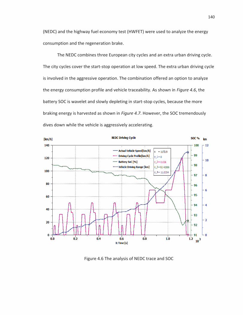
140
(NEDC) and the highway fuel economy test (HWFET) were used to analyze the energy
consumption and the regeneration brake.
The NEDC combines three European city cycles and an extra urban driving cycle.
The city cycles cover the start-stop operation at low speed. The extra urban driving cycle
is involved in the aggressive operation. The combination offered an option to analyze
the energy consumption profile and vehicle traceability. As shown in Figure 4.6, the
battery SOC is wavelet and slowly depleting in start-stop cycles, because the more
braking energy is harvested as shown in Figure 4.7. However, the SOC tremendously
dives down while the vehicle is aggressively accelerating.
Figure 4.6 The analysis of NEDC trace and SOC
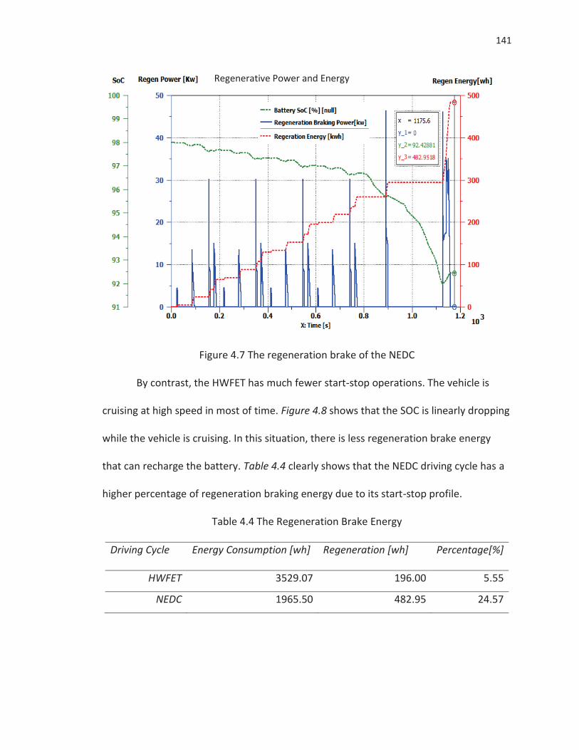
141
Figure 4.7 The regeneration brake of the NEDC
By contrast, the HWFET has much fewer start-stop operations. The vehicle is
cruising at high speed in most of time. Figure 4.8 shows that the SOC is linearly dropping
while the vehicle is cruising. In this situation, there is less regeneration brake energy
that can recharge the battery. Table 4.4 clearly shows that the NEDC driving cycle has a
higher percentage of regeneration braking energy due to its start-stop profile.
Table 4.4 The Regeneration Brake Energy
Driving Cycle Energy Consumption [wh] Regeneration [wh] Percentage[%]
HWFET 3529.07 196.00 5.55
NEDC 1965.50 482.95 24.57
Regenerative Power and Energy
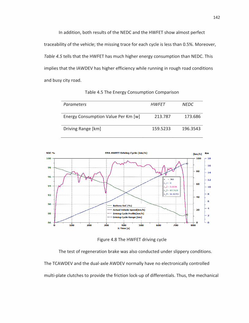
142
In addition, both results of the NEDC and the HWFET show almost perfect
traceability of the vehicle; the missing trace for each cycle is less than 0.5%. Moreover,
Table 4.5 tells that the HWFET has much higher energy consumption than NEDC. This
implies that the IAWDEV has higher efficiency while running in rough road conditions
and busy city road.
Table 4.5 The Energy Consumption Comparison
Parameters HWFET NEDC
Energy Consumption Value Per Km [w] 213.787 173.686
Driving Range [km] 159.5233 196.3543
Figure 4.8 The HWFET driving cycle
The test of regeneration brake was also conducted under slippery conditions.
The TCAWDEV and the dual-axle AWDEV normally have no electronically controlled
multi-plate clutches to provide the friction lock-up of differentials. Thus, the mechanical
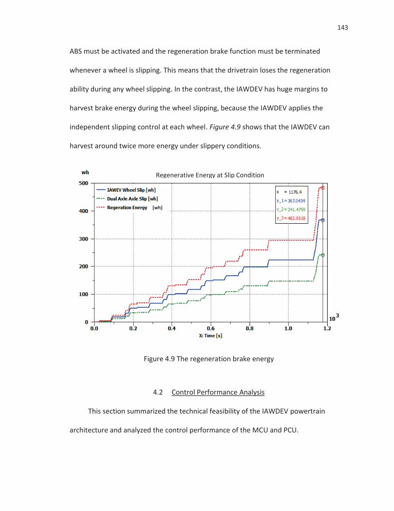
143
ABS must be activated and the regeneration brake function must be terminated
whenever a wheel is slipping. This means that the drivetrain loses the regeneration
ability during any wheel slipping. In the contrast, the IAWDEV has huge margins to
harvest brake energy during the wheel slipping, because the IAWDEV applies the
independent slipping control at each wheel. Figure 4.9 shows that the IAWDEV can
harvest around twice more energy under slippery conditions.
Figure 4.9 The regeneration brake energy
4.2 Control Performance Analysis
This section summarized the technical feasibility of the IAWDEV powertrain
architecture and analyzed the control performance of the MCU and PCU.
[wh]
Regenerative Energy at Slip Condition
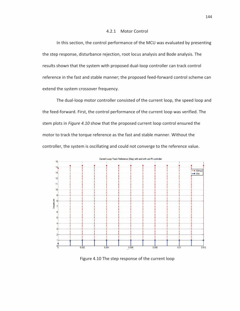
144
4.2.1 Motor Control
In this section, the control performance of the MCU was evaluated by presenting
the step response, disturbance rejection, root locus analysis and Bode analysis. The
results shown that the system with proposed dual-loop controller can track control
reference in the fast and stable manner; the proposed feed-forward control scheme can
extend the system crossover frequency.
The dual-loop motor controller consisted of the current loop, the speed loop and
the feed-forward. First, the control performance of the current loop was verified. The
stem plots in Figure 4.10 show that the proposed current loop control ensured the
motor to track the torque reference as the fast and stable manner. Without the
controller, the system is oscillating and could not converge to the reference value.
Figure 4.10 The step response of the current loop
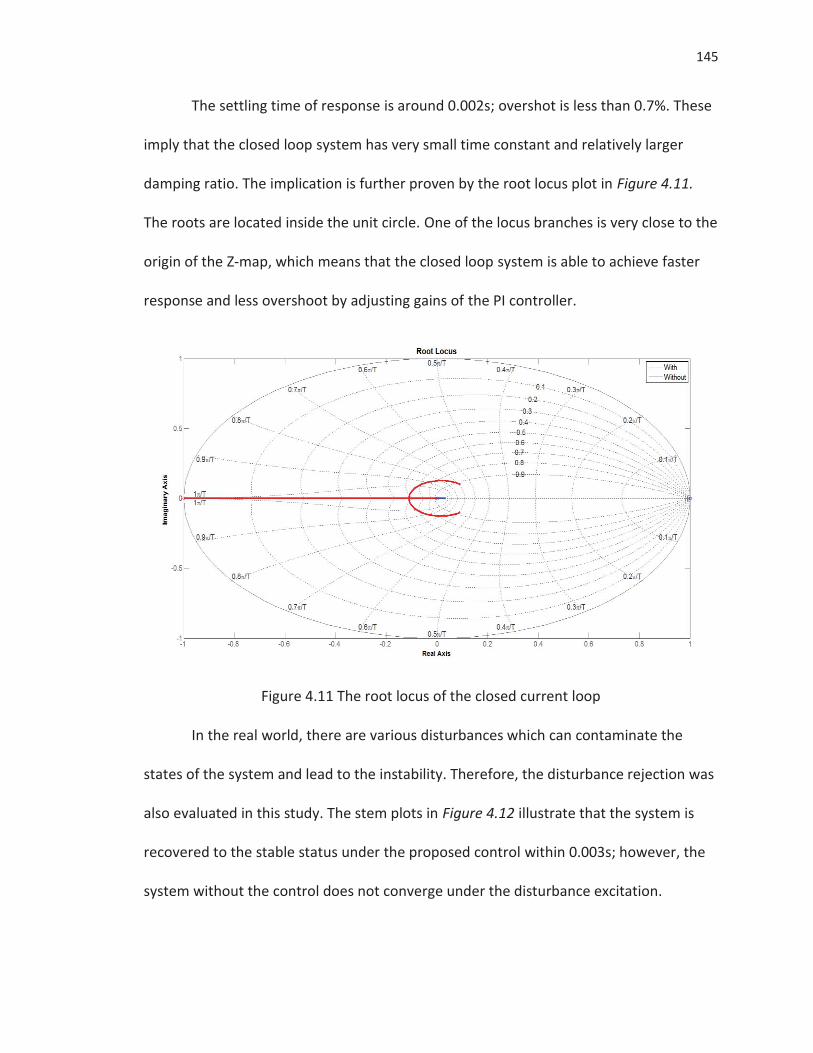
145
The settling time of response is around 0.002s; overshot is less than 0.7%. These
imply that the closed loop system has very small time constant and relatively larger
damping ratio. The implication is further proven by the root locus plot in Figure 4.11.
The roots are located inside the unit circle. One of the locus branches is very close to the
origin of the Z-map, which means that the closed loop system is able to achieve faster
response and less overshoot by adjusting gains of the PI controller.
Figure 4.11 The root locus of the closed current loop
In the real world, there are various disturbances which can contaminate the
states of the system and lead to the instability. Therefore, the disturbance rejection was
also evaluated in this study. The stem plots in Figure 4.12 illustrate that the system is
recovered to the stable status under the proposed control within 0.003s; however, the
system without the control does not converge under the disturbance excitation.
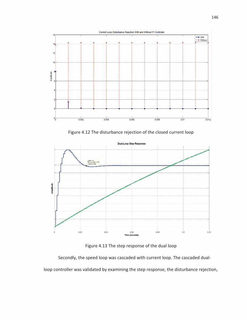
146
Figure 4.12 The disturbance rejection of the closed current loop
Figure 4.13 The step response of the dual loop
Secondly, the speed loop was cascaded with current loop. The cascaded dual-
loop controller was validated by examining the step response, the disturbance rejection,
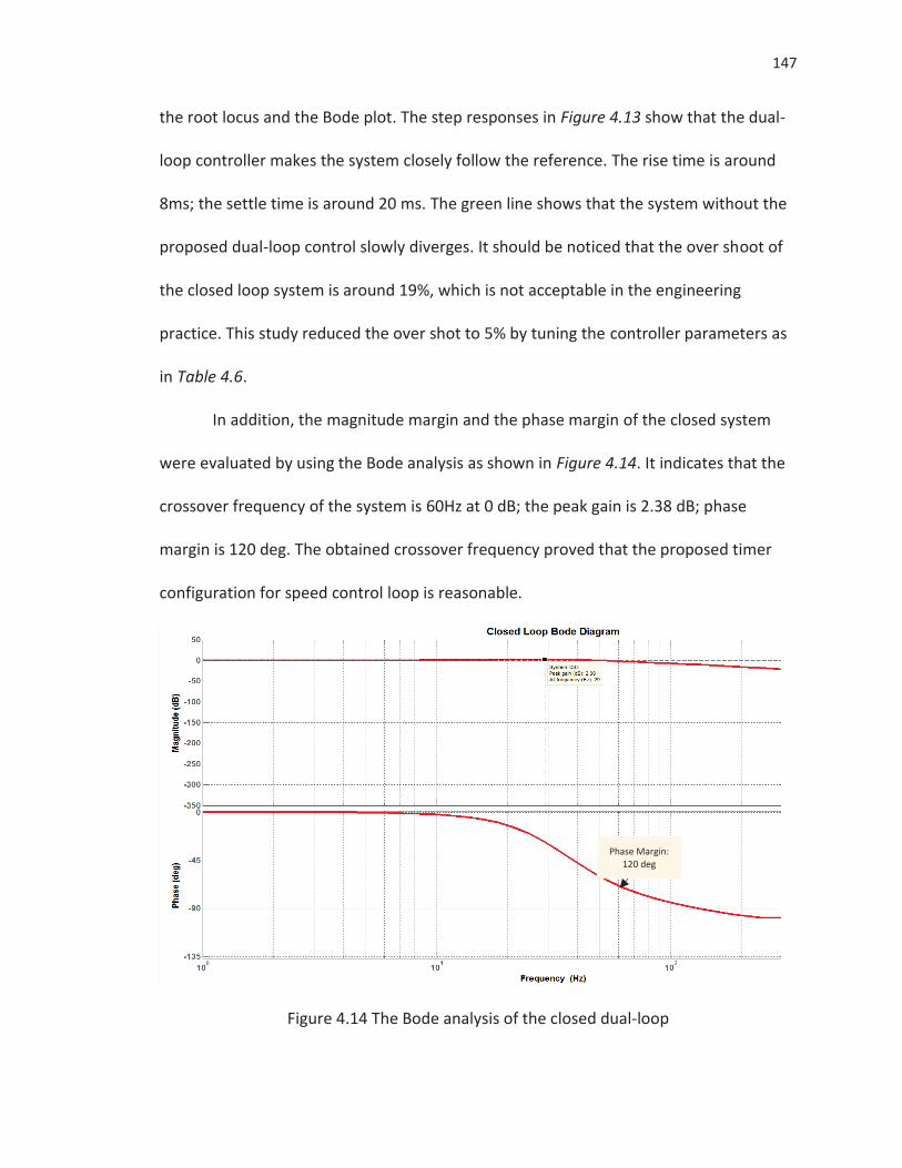
147
the root locus and the Bode plot. The step responses in Figure 4.13 show that the dual-
loop controller makes the system closely follow the reference. The rise time is around
8ms; the settle time is around 20 ms. The green line shows that the system without the
proposed dual-loop control slowly diverges. It should be noticed that the over shoot of
the closed loop system is around 19%, which is not acceptable in the engineering
practice. This study reduced the over shot to 5% by tuning the controller parameters as
in Table 4.6.
In addition, the magnitude margin and the phase margin of the closed system
were evaluated by using the Bode analysis as shown in Figure 4.14. It indicates that the
crossover frequency of the system is 60Hz at 0 dB; the peak gain is 2.38 dB; phase
margin is 120 deg. The obtained crossover frequency proved that the proposed timer
configuration for speed control loop is reasonable.
Figure 4.14 The Bode analysis of the closed dual-loop
Phase Margin: 120 deg
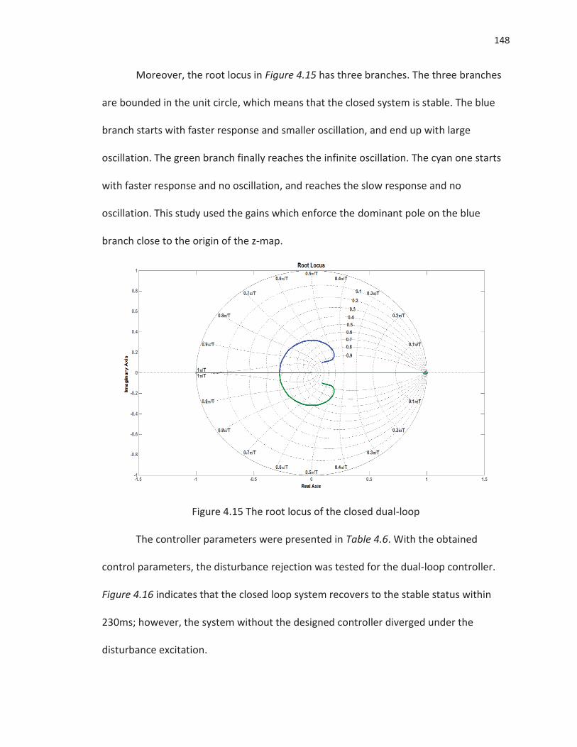
148
Moreover, the root locus in Figure 4.15 has three branches. The three branches
are bounded in the unit circle, which means that the closed system is stable. The blue
branch starts with faster response and smaller oscillation, and end up with large
oscillation. The green branch finally reaches the infinite oscillation. The cyan one starts
with faster response and no oscillation, and reaches the slow response and no
oscillation. This study used the gains which enforce the dominant pole on the blue
branch close to the origin of the z-map.
Figure 4.15 The root locus of the closed dual-loop
The controller parameters were presented in Table 4.6. With the obtained
control parameters, the disturbance rejection was tested for the dual-loop controller.
Figure 4.16 indicates that the closed loop system recovers to the stable status within
230ms; however, the system without the designed controller diverged under the
disturbance excitation.
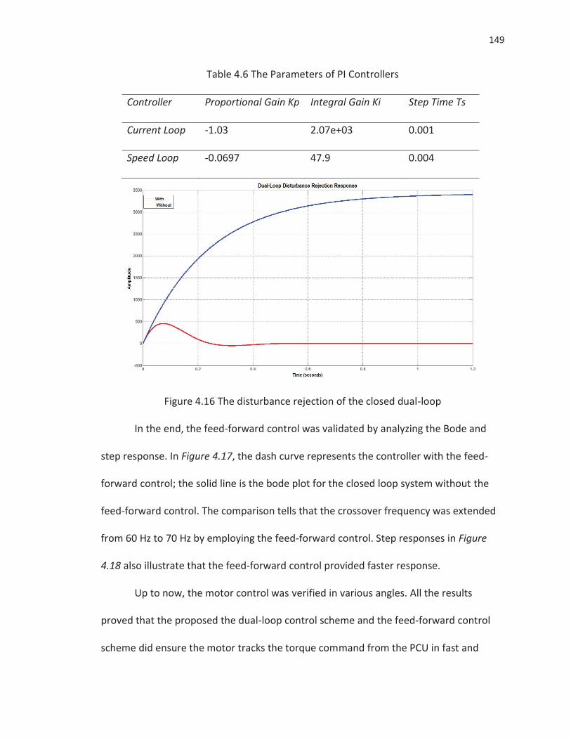
149
Table 4.6 The Parameters of PI Controllers
Controller Proportional Gain Kp Integral Gain Ki Step Time Ts
Current Loop -1.03 2.07e+03 0.001
Speed Loop -0.0697 47.9 0.004
Figure 4.16 The disturbance rejection of the closed dual-loop
In the end, the feed-forward control was validated by analyzing the Bode and
step response. In Figure 4.17, the dash curve represents the controller with the feed-
forward control; the solid line is the bode plot for the closed loop system without the
feed-forward control. The comparison tells that the crossover frequency was extended
from 60 Hz to 70 Hz by employing the feed-forward control. Step responses in Figure
4.18 also illustrate that the feed-forward control provided faster response.
Up to now, the motor control was verified in various angles. All the results
proved that the proposed the dual-loop control scheme and the feed-forward control
scheme did ensure the motor tracks the torque command from the PCU in fast and
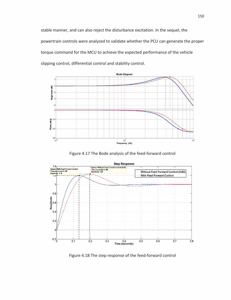
150
stable manner, and can also reject the disturbance excitation. In the sequel, the
powertrain controls were analyzed to validate whether the PCU can generate the proper
torque command for the MCU to achieve the expected performance of the vehicle
slipping control, differential control and stability control.
Figure 4.17 The Bode analysis of the feed-forward control
Figure 4.18 The step response of the feed-forward control
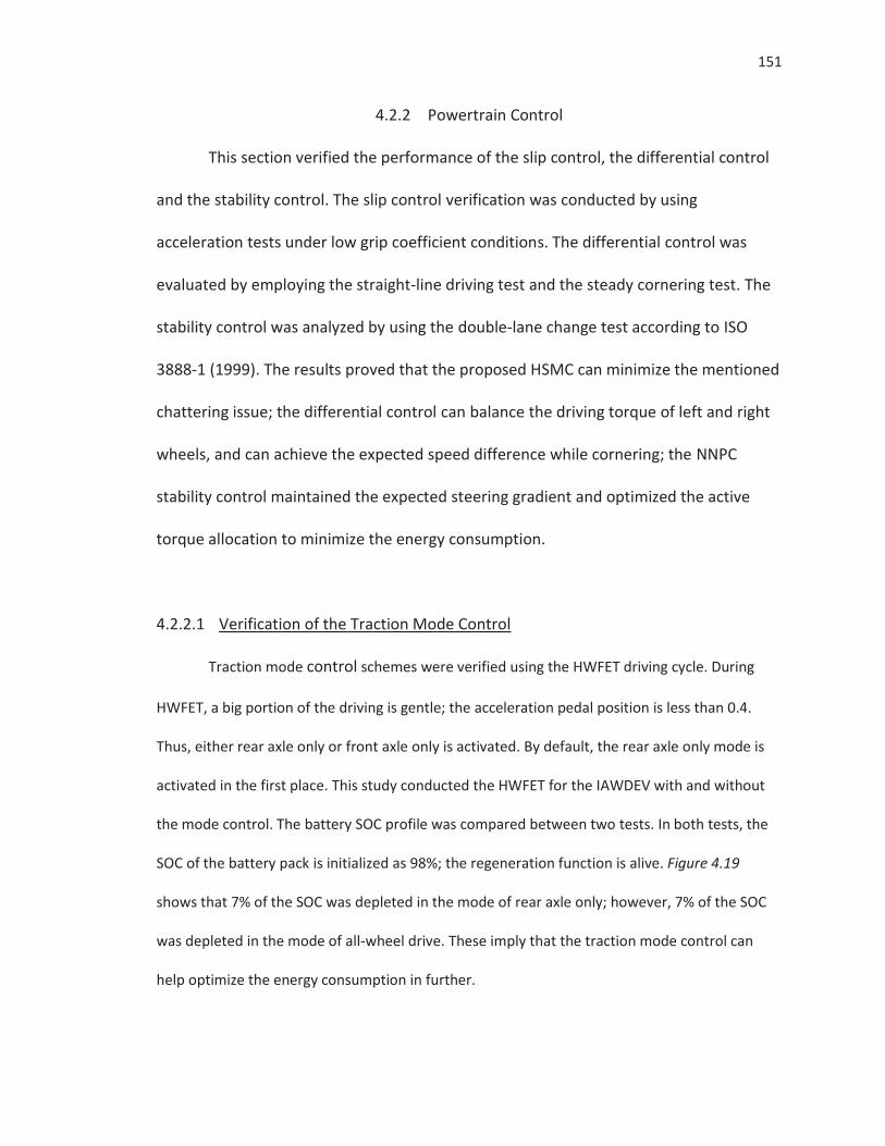
151
4.2.2 Powertrain Control
This section verified the performance of the slip control, the differential control
and the stability control. The slip control verification was conducted by using
acceleration tests under low grip coefficient conditions. The differential control was
evaluated by employing the straight-line driving test and the steady cornering test. The
stability control was analyzed by using the double-lane change test according to ISO
3888-1 (1999). The results proved that the proposed HSMC can minimize the mentioned
chattering issue; the differential control can balance the driving torque of left and right
wheels, and can achieve the expected speed difference while cornering; the NNPC
stability control maintained the expected steering gradient and optimized the active
torque allocation to minimize the energy consumption.
4.2.2.1 Verification of the Traction Mode Control
Traction mode control schemes were verified using the HWFET driving cycle. During
HWFET, a big portion of the driving is gentle; the acceleration pedal position is less than 0.4.
Thus, either rear axle only or front axle only is activated. By default, the rear axle only mode is
activated in the first place. This study conducted the HWFET for the IAWDEV with and without
the mode control. The battery SOC profile was compared between two tests. In both tests, the
SOC of the battery pack is initialized as 98%; the regeneration function is alive. Figure 4.19
shows that 7% of the SOC was depleted in the mode of rear axle only; however, 7% of the SOC
was depleted in the mode of all-wheel drive. These imply that the traction mode control can
help optimize the energy consumption in further.
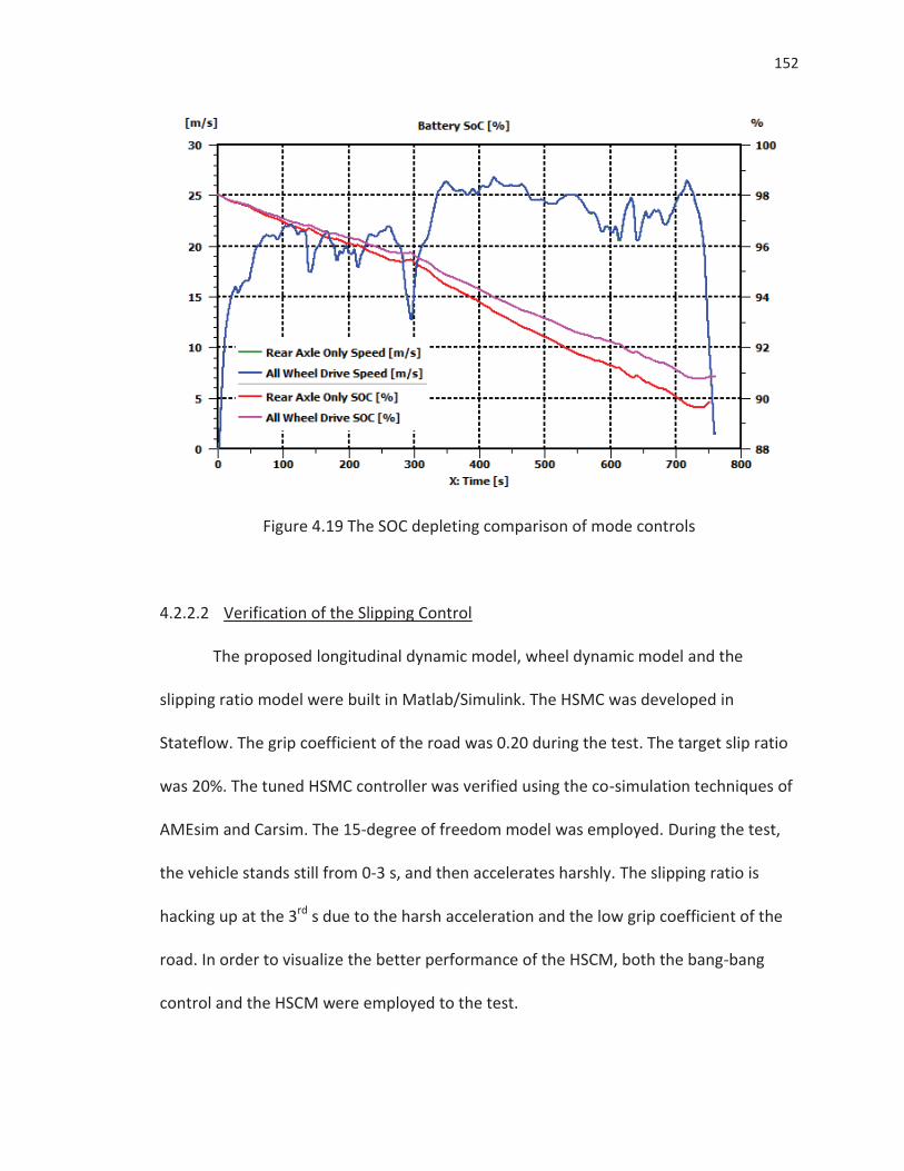
152
Figure 4.19 The SOC depleting comparison of mode controls
4.2.2.2 Verification of the Slipping Control
The proposed longitudinal dynamic model, wheel dynamic model and the
slipping ratio model were built in Matlab/Simulink. The HSMC was developed in
Stateflow. The grip coefficient of the road was 0.20 during the test. The target slip ratio
was 20%. The tuned HSMC controller was verified using the co-simulation techniques of
AMEsim and Carsim. The 15-degree of freedom model was employed. During the test,
the vehicle stands still from 0-3 s, and then accelerates harshly. The slipping ratio is
hacking up at the 3rd s due to the harsh acceleration and the low grip coefficient of the
road. In order to visualize the better performance of the HSCM, both the bang-bang
control and the HSCM were employed to the test.
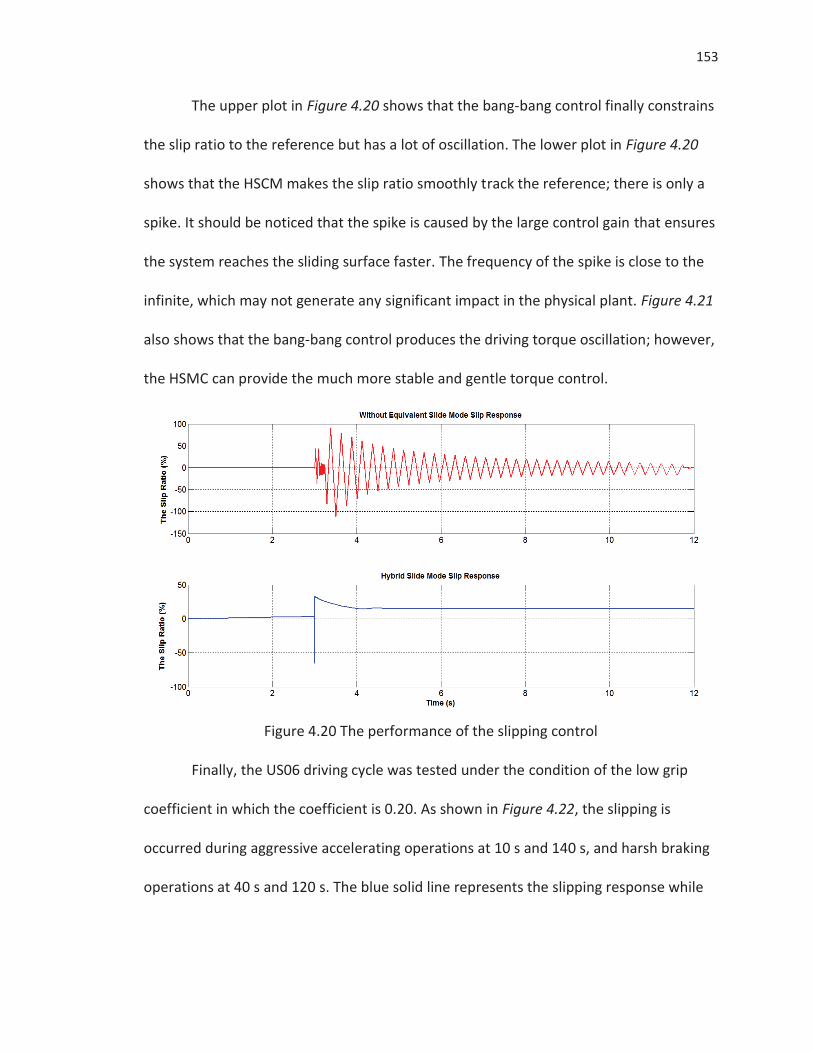
153
The upper plot in Figure 4.20 shows that the bang-bang control finally constrains
the slip ratio to the reference but has a lot of oscillation. The lower plot in Figure 4.20
shows that the HSCM makes the slip ratio smoothly track the reference; there is only a
spike. It should be noticed that the spike is caused by the large control gain that ensures
the system reaches the sliding surface faster. The frequency of the spike is close to the
infinite, which may not generate any significant impact in the physical plant. Figure 4.21
also shows that the bang-bang control produces the driving torque oscillation; however,
the HSMC can provide the much more stable and gentle torque control.
Figure 4.20 The performance of the slipping control
Finally, the US06 driving cycle was tested under the condition of the low grip
coefficient in which the coefficient is 0.20. As shown in Figure 4.22, the slipping is
occurred during aggressive accelerating operations at 10 s and 140 s, and harsh braking
operations at 40 s and 120 s. The blue solid line represents the slipping response while
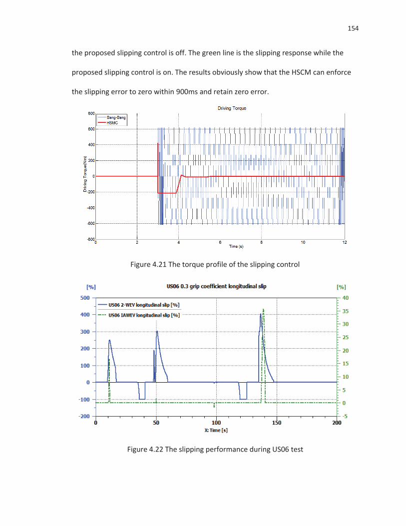
154
the proposed slipping control is off. The green line is the slipping response while the
proposed slipping control is on. The results obviously show that the HSCM can enforce
the slipping error to zero within 900ms and retain zero error.
Figure 4.21 The torque profile of the slipping control
Figure 4.22 The slipping performance during US06 test
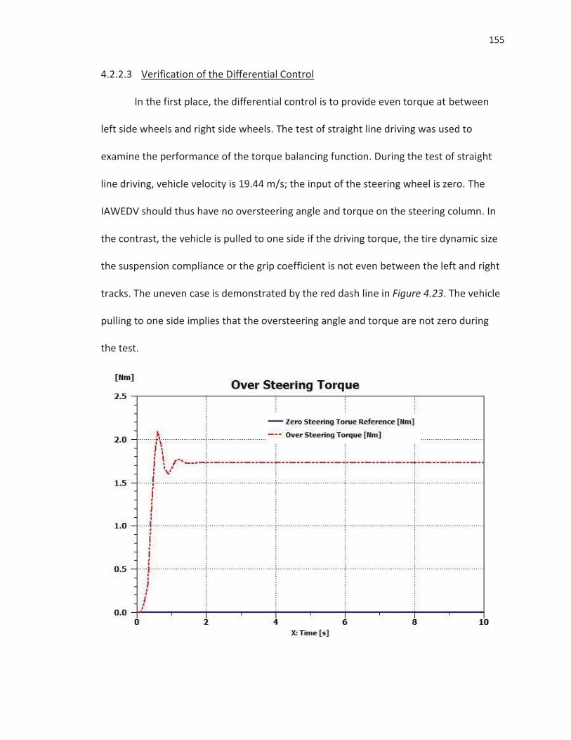
155
4.2.2.3 Verification of the Differential Control
In the first place, the differential control is to provide even torque at between
left side wheels and right side wheels. The test of straight line driving was used to
examine the performance of the torque balancing function. During the test of straight
line driving, vehicle velocity is 19.44 m/s; the input of the steering wheel is zero. The
IAWEDV should thus have no oversteering angle and torque on the steering column. In
the contrast, the vehicle is pulled to one side if the driving torque, the tire dynamic size
the suspension compliance or the grip coefficient is not even between the left and right
tracks. The uneven case is demonstrated by the red dash line in Figure 4.23. The vehicle
pulling to one side implies that the oversteering angle and torque are not zero during
the test.
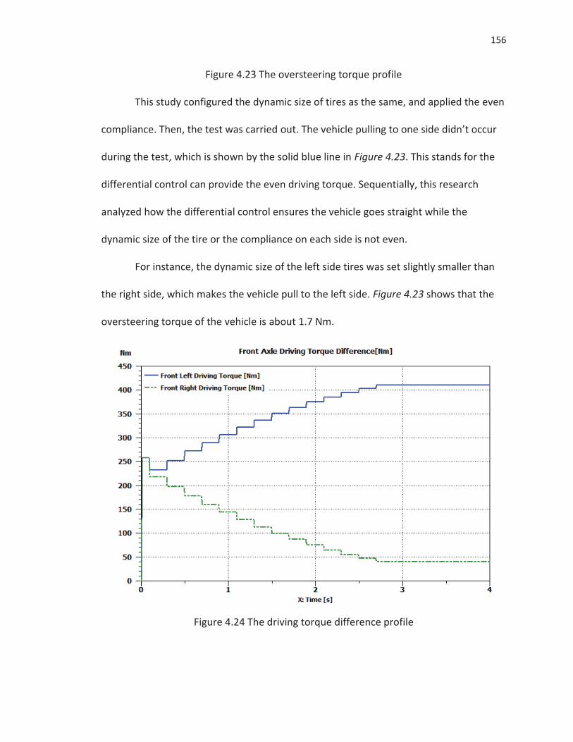
156
Figure 4.23 The oversteering torque profile
This study configured the dynamic size of tires as the same, and applied the even
compliance. Then, the test was carried out. The vehicle pulling to one side didn’t occur
during the test, which is shown by the solid blue line in Figure 4.23. This stands for the
differential control can provide the even driving torque. Sequentially, this research
analyzed how the differential control ensures the vehicle goes straight while the
dynamic size of the tire or the compliance on each side is not even.
For instance, the dynamic size of the left side tires was set slightly smaller than
the right side, which makes the vehicle pull to the left side. Figure 4.23 shows that the
oversteering torque of the vehicle is about 1.7 Nm.
Figure 4.24 The driving torque difference profile
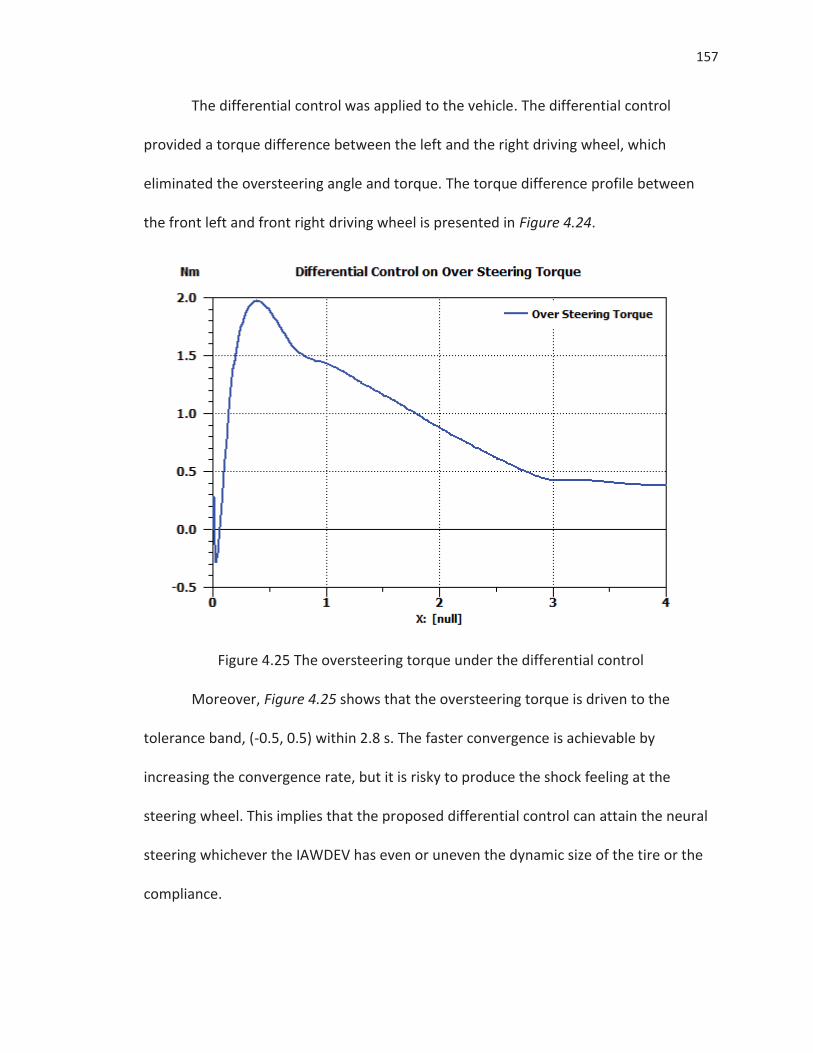
157
The differential control was applied to the vehicle. The differential control
provided a torque difference between the left and the right driving wheel, which
eliminated the oversteering angle and torque. The torque difference profile between
the front left and front right driving wheel is presented in Figure 4.24.
Figure 4.25 The oversteering torque under the differential control
Moreover, Figure 4.25 shows that the oversteering torque is driven to the
tolerance band, (-0.5, 0.5) within 2.8 s. The faster convergence is achievable by
increasing the convergence rate, but it is risky to produce the shock feeling at the
steering wheel. This implies that the proposed differential control can attain the neural
steering whichever the IAWDEV has even or uneven the dynamic size of the tire or the
compliance.
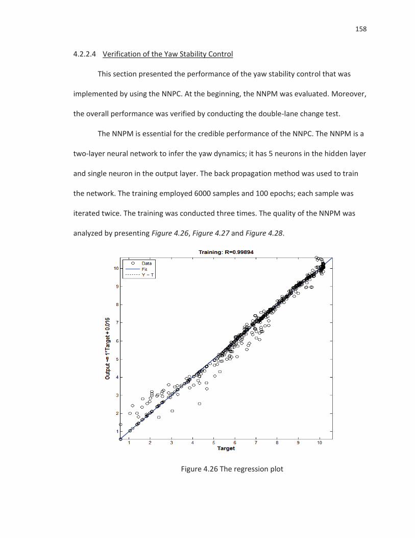
158
4.2.2.4 Verification of the Yaw Stability Control
This section presented the performance of the yaw stability control that was
implemented by using the NNPC. At the beginning, the NNPM was evaluated. Moreover,
the overall performance was verified by conducting the double-lane change test.
The NNPM is essential for the credible performance of the NNPC. The NNPM is a
two-layer neural network to infer the yaw dynamics; it has 5 neurons in the hidden layer
and single neuron in the output layer. The back propagation method was used to train
the network. The training employed 6000 samples and 100 epochs; each sample was
iterated twice. The training was conducted three times. The quality of the NNPM was
analyzed by presenting Figure 4.26, Figure 4.27 and Figure 4.28.
Figure 4.26 The regression plot
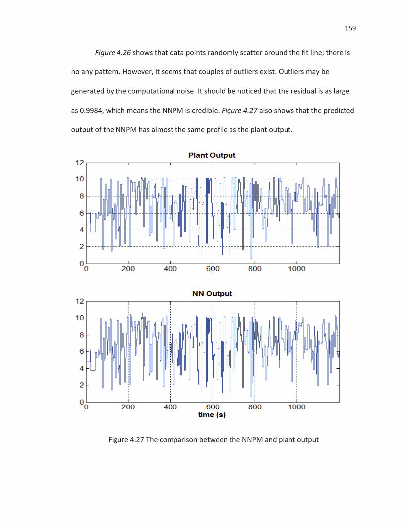
159
Figure 4.26 shows that data points randomly scatter around the fit line; there is
no any pattern. However, it seems that couples of outliers exist. Outliers may be
generated by the computational noise. It should be noticed that the residual is as large
as 0.9984, which means the NNPM is credible. Figure 4.27 also shows that the predicted
output of the NNPM has almost the same profile as the plant output.
Figure 4.27 The comparison between the NNPM and plant output
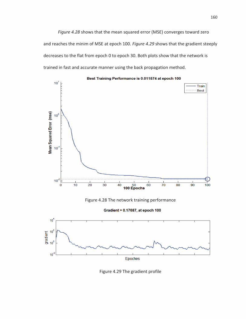
160
Figure 4.28 shows that the mean squared error (MSE) converges toward zero
and reaches the minim of MSE at epoch 100. Figure 4.29 shows that the gradient steeply
decreases to the flat from epoch 0 to epoch 30. Both plots show that the network is
trained in fast and accurate manner using the back propagation method.
Figure 4.28 The network training performance
Figure 4.29 The gradient profile
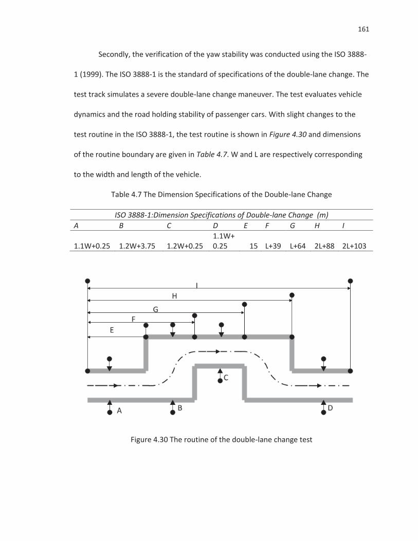
161
Secondly, the verification of the yaw stability was conducted using the ISO 3888-
1 (1999). The ISO 3888-1 is the standard of specifications of the double-lane change. The
test track simulates a severe double-lane change maneuver. The test evaluates vehicle
dynamics and the road holding stability of passenger cars. With slight changes to the
test routine in the ISO 3888-1, the test routine is shown in Figure 4.30 and dimensions
of the routine boundary are given in Table 4.7. W and L are respectively corresponding
to the width and length of the vehicle.
Table 4.7 The Dimension Specifications of the Double-lane Change
ISO 3888-1:Dimension Specifications of Double-lane Change (m) A B C D E F G H I
1.1W+0.25 1.2W+3.75 1.2W+0.25 1.1W+0.25 15 L+39 L+64 2L+88 2L+103
Figure 4.30 The routine of the double-lane change test
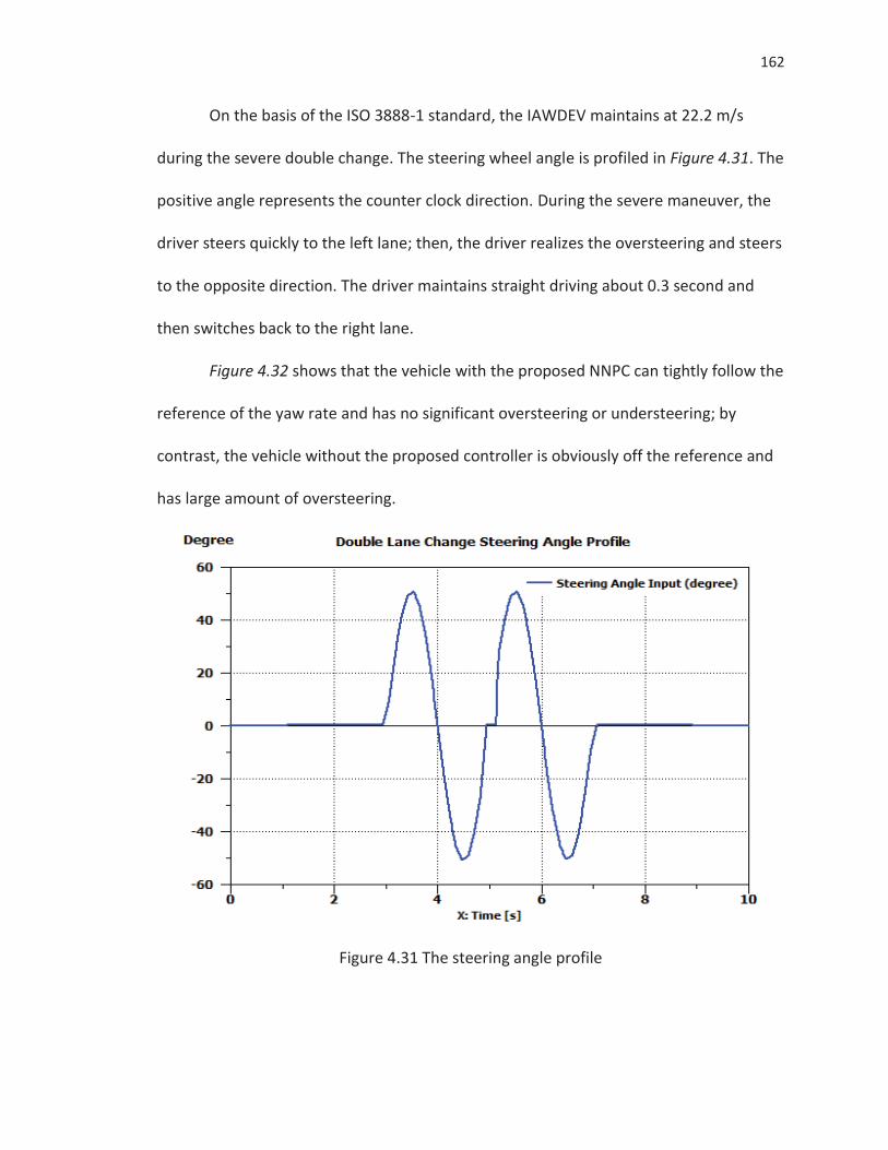
162
On the basis of the ISO 3888-1 standard, the IAWDEV maintains at 22.2 m/s
during the severe double change. The steering wheel angle is profiled in Figure 4.31. The
positive angle represents the counter clock direction. During the severe maneuver, the
driver steers quickly to the left lane; then, the driver realizes the oversteering and steers
to the opposite direction. The driver maintains straight driving about 0.3 second and
then switches back to the right lane.
Figure 4.32 shows that the vehicle with the proposed NNPC can tightly follow the
reference of the yaw rate and has no significant oversteering or understeering; by
contrast, the vehicle without the proposed controller is obviously off the reference and
has large amount of oversteering.
Figure 4.31 The steering angle profile
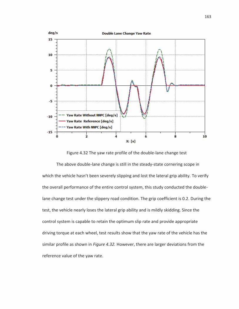
163
Figure 4.32 The yaw rate profile of the double-lane change test
The above double-lane change is still in the steady-state cornering scope in
which the vehicle hasn’t been severely slipping and lost the lateral grip ability. To verify
the overall performance of the entire control system, this study conducted the double-
lane change test under the slippery road condition. The grip coefficient is 0.2. During the
test, the vehicle nearly loses the lateral grip ability and is mildly skidding. Since the
control system is capable to retain the optimum slip rate and provide appropriate
driving torque at each wheel, test results show that the yaw rate of the vehicle has the
similar profile as shown in Figure 4.32. However, there are larger deviations from the
reference value of the yaw rate.
164
4.3 Summary
This chapter provided comprehensive verifications of the powertrain
architecture and control performance. The obtained data indicated that the proposed
design has less weight in the contrast to other powertrain architectures in previous
studies. The data and plots obtained by using MIL and HIL methods provided creditable
evidences that the designed powertrain can meet the predefined VTS; in the meanwhile,
the control schemes can achieve better functional performances than the mechanical
linked all-wheel drive system. The next chapter reports implications and potential
applications of this research. The possible future work is also discussed.
165
CHAPTER 5. CONCLUSION
Previous studies have investigated the TCWDEV and the dual-axle AWDEV to
balance concerns about energy consumption, drivability and stability. However, the
architectures have been suffering some intrinsic drawbacks including drivetrain winding
up, larger drivetrain weight and more mounting space. They also have limitations on
regeneration brake under slippery road conditions. This study aimed to solve these
issues by developing the IAWDEV powertrain and its control system. The IAWDEV is
powered by four independent PMSMs; its energy storage system employs high power Li-
ion battery. The motors were accurately sized by using the acceleration and cruising
requirements in the predefined VTS. The battery capacity was precisely estimated by
utilizing the cruising duration at 3% grade.
The model-based verification results proved that the proposed architecture
achieved better performance than the requirements in the VTS, and the discussed sizing
methods were creditable to decide the operation envelop of components. In addition,
the IAWDEV can harvest more energy under slippery conditions. This study didn’t only
discuss IAWDEV powertrain architecture in detail and deeply analyze the powertrain
energy consumption and the vehicle drivability, but also investigated the wheel slip
166
control, the differential control and the yaw stability control by using extra control
freedoms that the IAWDEV provided.
The controls were carried out by applying active torque to each driving wheel.
Based on the comprehensive evaluations, the performance of control schemes
proposed in this study met the expectations. The slip control increased the convergence
speed of the system trajectory and also retained the slide mode; it also prevented the
Zeno oscillation occurred in the traditional anti-slip control. The braking control of each
wheel harvested most of braking energy that is up to 6% of the overall vehicle energy
consumption. The differential control achieved different rotation speed between
outside wheels and inside wheels, and delivered even torque on each side. The yaw
stability control ensured the yaw response tracks the yaw reference in the fast and
stable manner.
All these evaluation results indicate that the proposed powertrain architecture
and its control system can replace the traditional mechanical links, and can obtain
better functional performance in more flexible ways. Most notably, to the author’s
knowledge, this is the first study to investigate the IAWDEV powertrain design and its
controls in the systematic manner. This study provided compelling evidences that the
functions achieved by complicated mechanical devices can be carried out by control
schemes of IAWDEV.
However, some limitations are worth noting. Although the weight transfer was
considered while conducting the slipping control and the yaw stability control, the
impact of suspension compliance wasn’t accounted. Future work should therefore
167
include follow-up work to evaluate whether the proposed control performance are
retained if the suspension system compliance is changed while the vehicle is cornering.
Even though the credible tools were employed as the verification platform, the tools are
still lack of some constraints in the real world. Future work should also include the
follow-up work to build up a physical prototype to verify whether the proposed IAWDEV
and its controls are functioning as expected under various constraints in the physical
world.
What is more, the PMSM and the Li-ion battery are sensitive to the operating
temperature. Thus, the novel cooling system for the IAWDEV powertrain should be
carefully investigated in the future study. In addition, this research discussed the
traction mode and faults mode controls, but didn’t investigate the fault mitigation
strategy. The fault mitigation strategy could be deeply studied in the future research.

LIST OF REFERENCES
168
LIST OF REFERENCES
Akin, B., & Bhardwaj, M. (2013). Sensorless Field Oriented Control of 3-Phase Permanent Magnet Synchronous Motors (pp. 1–43).
American Association of State Highway and Transportation Officials (2001). A Policy on Geometric Design of Highways and Streets. Washinton D.C.: U.S. GoverNment Printing Office
Ang, K., Chong, G., & Li, Y. (2005). PID control system analysis, design, and technology. Control Systems Technology, IEEE …, 13(4), 559–576. Retrieved from http://ieeexplore.ieee.org/xpls/abs_all.jsp?arnumber=1453566
Anwar, S. (2005). Generalized predictive control of yaw dynamics of a hybrid brake-by-wire equipped vehicle. Mechatronics, 15(9), 1089–1108. doi:10.1016/j.mechatronics.2005.06.006
Arnett, M., Rizzoni, G., & Heydinger, G. (2008). Implementation of an Electric All-Wheel Drive (eAWD) System. SAE Technical Paper, 2008(724), 776–790. Retrieved from http://papers.sae.org/2008-01-0599/
Astrom, K. J., & Hagglund, T. (1995). PID controllers: Theory, design, and tuning. Research Triangle Park, NC: Instrument Society ofAmerica.
Benini, L., Castelli, G., Macii, a., Macii, E., Poncino, M., & Scarsi, R. (2001). Discrete-time battery models for system-level low-power design. IEEE Transactions on Very Large Scale Integration (VLSI) Systems, 9(5), 630–640. doi:10.1109/92.953497
Bhardwaj, M. (2013). Sensored Field Oriented Control of 3-Phase Permanent Magnet Synchronous Motors.
Bian, M., Chen, L., Luo, Y., & Li, K. (2014). A Dynamic Model for Tire / Road Friction Estimation under Combined Longitudinal / Lateral Slip Situation Analysis on Dugoff Tire Model. doi:10.4271/2014-01-0123.Copyright

169
Biglarbegian, M., Melek, W., & Golnaraghi, F. (2007). Design of a Novel Fuzzy Controller to Enhance Stability of Vehicles. NAFIPS 2007 - 2007 Annual Meeting of the North American Fuzzy Information Processing Society, 410–414. doi:10.1109/NAFIPS.2007.383874
Bosch Automotive Handbook (6th ed.) (2004). Postfach, Plochingen: Robert Bosh Gmbh.
Brogan, W.L. (1991). Modern Control Theory (3rd ed.). Englewood Cliffs, NJ: Prentice-Hall, Inc.
Burghardt, M.D., Harbach, A.J. (1993), Engineering Thermaldynamics (4th ed.). New York, Ny: HarperCollins College Publishers.
Chu, H., & Lin, W. (2010). Neural-network synthesis of integrated brake controller of electrical vehicle. 2010 5th IEEE Conference on Industrial Electronics and Applications, 29–34. doi:10.1109/ICIEA.2010.5516740
Cirrincione, M., Pucci, M., & Vitale, G. (2012). Power Converters and AC Electrical Drives with Linear Neural Networks (CRC Press.). London. Retrieved from http://books.google.com/books?hl=en&lr=&id=mjuRkz1PA0gC&oi=fnd&pg=PP1&dq=Power+Converters+and+AC+Electrical+Drives+with+Linear+Neural+Networks&ots=d2HnKOzEqJ&sig=hatcyUYqhqJhvIZu6b0cQgr1Dvw
Cybenko, G. (1989). Approximation by superpositions of a sigmoidal function. Mathematics of Control, Signals, and Systems (MCSS), 2(4):303–314.
King-Hele, D. (2002). Erasmus Darwin's improved design for steering carriages and cars.The Royal Society Jounal of the History of Science, 56(1), 41–62. doi:10.1098/rsnr.2002.0166
Dick, W. (1995). All-wheel and Four-wheel-drive Vehicle Systems. SAE Technical Paper, (November 1995). Retrieved from http://papers.sae.org/952600/
Draou, A. (2013). A Simplified Sliding Mode Controlled Electronic Differential for an Electric Vehicle with Two Independent Wheel Drives. Energy and Power Engineering, 05(06), 416–421. doi:10.4236/epe.2013.56044
Ellis, G. (2003).Control System Design Guide (3rd ed.). San Diego, CA: Elsevier Inc.
Esmailzadeh, E., Vossoughi, G. R., & Goodarzi, a. (2001). Dynamic Modeling and Analysis of a Four Motorized Wheels Electric Vehicle. Vehicle System Dynamics, 35(3), 163–194. doi:10.1076/vesd.35.3.163.2047
170
Gao, L., Liu ,S., & Dougal,R. A.(2002). Dynamic Lithium-Ion Battery Model for System Simulation.IEEE Transactions on Components and Packaging Technologies, vol. 25 , pp. 495-505.
Gao, X., Yu, Z., & Xu, T. (2008). Longitudinal Velocity Estimation of Electric Vehicle with 4 In-wheel Motors. SAE Technical Paper, 2008(724). Retrieved from http://papers.sae.org/2008-01-0605/
Geng, C., & Mostefai, L. (2009). Direct yaw-moment control of an in-wheel-motored electric vehicle based on body slip angle fuzzy observer. … , IEEE Transactions on, 56(5), 1411–1419. Retrieved from http://ieeexplore.ieee.org/xpls/abs_all.jsp?arnumber=4776489
Green M.(2009),Perception-Reaction Time: Is Olson (and Sivak) All You Need to Know?, collision, 4(2):88-93. Retrieved from: http://trid.trb.org/view.aspx?id=913048
Gillespie, T.D. (1992). Fundamentals Of Vehicle Dynamics (1st ed.). Warrendale, PA: Society of Automotive Engineer, Inc.
Goodarzi, A., & Esmailzadeh, E. (2007). Design of a VDC System for All-Wheel Independent Drive Vehicles. IEEE/ASME Transactions on Mechatronics, 12(6), 632–639. doi:10.1109/TMECH.2007.910075
Hanselman, D. (1994). Brushless permanent-magnet motor design. McGraw-Hill. Retrieved from http://scholar.google.com/scholar?hl=en&btnG=Search&q=intitle:Brushless+Permanent-Magnet+Motor+Design#0
Hartani, K., & Bourahla, M. (2009). Electronic Differential with Direct Torque Fuzzy Control. Turkish Journal of Electrical Engineering and Computer Sciences, 17(1). doi:10.3906/elk-0801-1
Hartani, K., Miloud, Y., & Miloudi, A. (2010). Electric Vehicle stability with rear Electronic differential Traction. International Symposium on Enviroment Friendly Energies in Electrcal Appllcations, (November), 1–5. Retrieved from http://www.umc.edu.dz/vf/proceeding/efeea-2010/Topic_2/PS-ES03.pdf
Hava, A.M., Sul, S., S., Kerman, R.J. (1999), Dynamic Overmodulation Characteristics of Triangle Intersection PWM Methods, IEEE Trans. Ind. Appl., vol 35, no.4.
171
Horn, H., Dale, W. (2012). Planetary gears-A review of basic design criteria and new options for sizing, machine design. Retrieve from: http://machinedesign.com/mechanical-drives/planetary-gears-review-basic-design-criteria-and-new-options-sizing
ISO 3888-1 (1999). Passenger cars--Test track for a severe lane-change maneuver--Part 1: Double lane-change. International Standards Organization.
Kim, D., Hwang, S., & Kim, H. (2008). Vehicle Stability Enhancement of Four-Wheel-Drive Hybrid Electric Vehicle Using Rear Motor Control. IEEE Transactions on Vehicular Technology, 57(2), 727–735. doi:10.1109/TVT.2007.907016
Kriesel, D. (2007). A Brief Introduction to Neural Networks. Retrieved from: http://dkriesel.com/en/science/neural_networks
Lanier, T. (2005). All-wheel drive electric vehicle. US Patent App. 10/724,241, 1(19). Retrieved from http://www.google.com/patents/US20050115748
Lee H, Utkin VI. (2006). Chattering Analysis. Advances in Variable Structure and Sliding Mode Control, London: Springer-Verlag, 107–121.
Li, F., Wang, J., & Liu, Z. (2009). Fuzzy-Logic-Based Controller Design for Four-wheel-drive Electric Vehicle Yaw Stability Enhancement. 2009 Sixth International Conference on Fuzzy Systems and Knowledge Discovery, 116–120. doi:10.1109/FSKD.2009.827
Li, J., Wu, D., Zhang, X., & Gao, S. (2010). A new permanent-magnet vernier in-wheel motor for electric vehicles. Vehicle Power and Propulsion. Retrieved from http://ieeexplore.ieee.org/xpls/abs_all.jsp?arnumber=5729062
Liao, G. Y., Weber, T. R., & Pfaff, D. P. (2004). Modelling and analysis of Powertrain hybridization on all-wheel drive sport utility vehicles. Proceedings of the Institution of Mechanical Engineers, Part D: Journal of Automobile Engineering, 218(10), 1125–1134. doi:10.1177/095440700421801007
Magallan, G., Angelo, C., Bisheirmer, G., & Garcia, G. (2008). A neighborhood electric vehicle with electronic differential traction control. In Proceedings - 34th Annual Conference of the IEEE Industrial Electronics Society (pp. 2757–2763). doi:10.1109/IECON.2008.4758395
Mclaughlin, R. T., Dõsouza, E., & Warwick, K. H. T. Ð. (n.d.). CAN Bus Performance Analysis of DeviceNet I / O Connection Services (pp. 16–24).
172
Nash, J. N. (1997). Direct torque control, induction motor vector control without an encoder. IEEE Transactions on Industry Applications, 33(2), 333–341. doi:10.1109/28.567792
Quang, N., & Dittrich, J. (2008). Vector control of three-phase AC machines. Retrieved from http://link.springer.com/content/pdf/10.1007/978-3-540-79029-7.pdf
Rahman, K. M., Patel, N. R., Ward, T. G., Nagashima, J. M., Caricchi, F., & Crescimbini, F. (2006). Application of Direct-Drive Wheel Motor for Fuel Cell Electric and Hybrid Electric Vehicle Propulsion System. IEEE Transactions on Industry Applications, 42(5), 1185–1192. doi:10.1109/TIA.2006.880886
Ravi, A., & Palani, S. (2013). Robust Electronic Differential Controller for an Electric Vehicle. American Journal of Applied Sciences, 10(11), 1356–1362. doi:10.3844/ajassp.2013.1356.1362
SAE J670e (2008). Vehicle Dynamics Terminology. Warrendale, PA: Society of Automotive Engineer, Inc.
Sayers M. Standard Terminology for Vehicle DyaNmics Simulations. Retrieved from http://mecara.fpms.ac.be/grasmech/StandardTerminologyForVehicleDynamicsSimulation.pdf
Sheidaei, F., Sedighizadeh, M., Mohseni-Zonoozi, S. H., & Alinejad-Beromi, Y. (2007). A fuzzy logic direct torque control for induction motor sensorless drive.. UPEC 2007. (1), 197–202. Retrieved from http://ieeexplore.ieee.org/xpls/abs_all.jsp?arnumber=4468946
Sinkaram, C., Rajakumar, K., & Asirvadam, V. (2012). Modeling battery management system using the lithium-ion battery. 2012 IEEE International Conference on Control System, Computing and Engineering, 50–55. doi:10.1109/ICCSCE.2012.6487114
Sivak, M., Flannagan, M., Sato, T., Traube, E., & Aoki, M. (1994). Reaction times to neon, LED, and fast incandescent brake lamps. Ergonomics, 37(6), 989–994. doi:10.1080/00140139408963712
Tahami, F., Farhangi, S., & Kazemi, R. (2004). A Fuzzy Logic Direct Yaw-Moment Control System for All-wheel drive Electric Vehicles. Vehicle System Dynamics, 41(3), 203–221. doi:10.1076/vesd.41.3.203.26510
173
Takahashi, I., & Noguchi, T. (1986). A New Quick-Response and High-Efficiency Control Strategy of an Induction Motor. IEEE Transactions on Industry Applications, IA-22(5), 820–827. doi:10.1109/TIA.1986.4504799
Taoutaou, D., Puerto, R., Ortega, R., & Loron, L. (1997). A new field-oriented discrete-time controller for current-fed induction motors. Control Engineering Practice, 5(2), 209–217. doi:10.1016/S0967-0661(97)00227-X
Toliyat, H.A. (2008). Proceedings from 34th IEEE IECON: Recent advances and applications of power electronics and motor drives—Electric machines and motor drives., pp. 34–36
Toman, J., Kerlin, T., & Singule, V. (2011). APPLICATION OF THE V-CYCLE DEVELOPMENT. Engineering MECHANICS, 18(5), 297–306.
Vora, A., Wu, H., Wang, C., Qian, Y., Shaver, G., Motevalli, V., ... & Zhang, H. (2014). Development of a SIL, HIL and Vehicle Test-Bench for Model-Based Design and Validation of Hybrid Powertrain Control Strategies (No. 2014-01-1906). SAE Technical Paper.
Wang, R., Chen, Y., Feng, D., Huang, X., & Wang, J. (2011). Development and performance characterization of an electric ground vehicle with independently actuated in-wheel motors. Journal of Power Sources, 196(8), 3962–3971. doi:10.1016/j.jpowsour.2010.11.160
Wang, R., Zhang, H., & Wang, J. (2014). Linear parameter-varying controller design for four-wheel independently actuated electric ground vehicles with active steering systems. IEEE Transactions on Control Systems Technology, 22(4), 1281–1296. Retrieved from http://ieeexplore.ieee.org/xpls/abs_all.jsp?arnumber=6589992
Watterson, C. (2013). Controller Area Network (CAN) Implementation Guide (pp. 1–16). Norwood.
Wu, H., Zhang, H., Motevalli, V., Qian, Y., & Wolfe, A. (2013). Hybrid Electric Vehicle Powertrain Controller Development Using Hardware in the Loop Simulation (No. 2013-01-0156). SAE Technical Paper.
Young, M., Member, S., Molen, G. M., Member, S., Oglesby, D., Crawford, K., … Phillips, S. (2007). The Design and Development of a Through-the- Road Parallel Diesel Electric Hybrid I5lVM60, 511–518.
174
Zanten, A., Erhardt R., & Lutz, A. (1990) Measurement and simulation of transients in long-tudinal and lateral tire forces, Proc. of the International Congress & Exposition, USA, Detroit, vol. 99, no. 6, pp. 300–318.
Zhao, Y., Zhang, Y., & Zhao, Y. (2009). Stability Control System for Four-in-Wheel-Motor Drive Electric Vehicle. 2009 Sixth International Conference on Fuzzy Systems and Knowledge Discovery, 171–175. doi:10.1109/FSKD.2009.582
Zhiping, Y., Qiuqin, Y., & Yong, Y. (2012). Induction Motor Speed Control Based on Model Reference. Procedia Engineering, 29, 2376–2381. doi:10.1016/j.proeng.2012.01.318
Zumbahlen, H.(Ed) (2007). Basic linear design. Norwood, MA: Analog Devices Inc.

APPENDICES
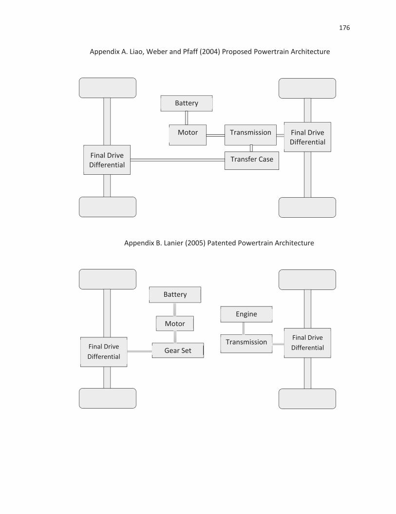
176
Appendix A. Liao, Weber and Pfaff (2004) Proposed Powertrain Architecture
Appendix B. Lanier (2005) Patented Powertrain Architecture
Motor
Transfer Case
Transmission
Battery
Final Drive Differential
Final Drive Differential
Motor
Gear Set Transmission
Battery
Engine
Final Drive Differential
Final Drive Differential
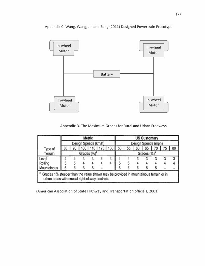
177
Appendix C. Wang, Wang, Jin and Song (2011) Designed Powertrain Prototype
Appendix D. The Maximum Grades for Rural and Urban Freeways
(American Association of State Highway and Transportation officials, 2001)
In-wheel Motor
In-wheel Motor
In-wheel Motor
Battery
In-wheel Motor
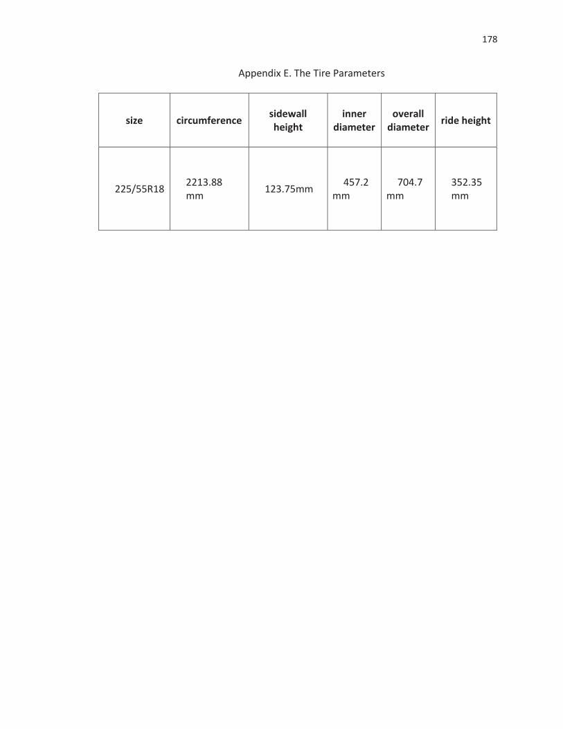
178
Appendix E. The Tire Parameters
size circumference sidewall height
inner diameter
overall diameter ride height
225/55R18 2213.88 mm
123.75mm 457.2
mm 704.7
mm 352.35 mm