Embed Size (px)
Citation preview

Minimax-distance criterion forspace-filling design:
evaluation, optimisation and construction of asubmodular alternative
Luc Pronzato
Université Côte d’Azur, CNRS, I3S, France

1) Introduction
1) Introduction & motivation
Ultimate objective = approximation, interpolationà approximate a function f : x ∈X ⊂ Rd −→ R,
(with X compact: typically, X = [0, 1]d)à Choose n points Xn = {x1, . . . , xn} ∈X n (the design)
where to evaluate f (no repetition)
Favourite design criterion = minimaxà minimise ΦmM(Xn) = maxx∈X mini=1,...,n ‖x− xi‖ (`2-distance)
= maxx∈X d(x,Xn)= dH(X ,Xn) (Hausdorff distance, `2)= dispersion of Xn in X (Niederreiter, 1992, Chap. 6)
Optimal n-point design X∗n Ô ΦmM-efficiency = Φ∗mM,n
ΦmM (Xn) ∈ (0, 1]
with Φ∗mM,n = ΦmM(X∗n )
Luc Pronzato (CNRS) Minimax-distance: evaluation & optimisation SAMO’2016, Dec. 2, 2016 2 / 49

1) Introduction
1 X and Xn ∈X n given, how to evaluate ΦmM(Xn)?
2 How to minimise ΦmM(Xn) with respect to Xn ∈X n?3 Suppose that n is not completely decided yet, we only know that
nmin ≤ n ≤ nmax (we may decide to stop before nmax evaluations of f )
How to obtain high efficiency for all nested designs Xn, with nmin ≤ n ≤ nmax?(SIAM UQ, Lausanne, April 5–8 2016)
Luc Pronzato (CNRS) Minimax-distance: evaluation & optimisation SAMO’2016, Dec. 2, 2016 3 / 49

1) Introduction
1 X and Xn ∈X n given, how to evaluate ΦmM(Xn)?2 How to minimise ΦmM(Xn) with respect to Xn ∈X n?
3 Suppose that n is not completely decided yet, we only know thatnmin ≤ n ≤ nmax (we may decide to stop before nmax evaluations of f )
How to obtain high efficiency for all nested designs Xn, with nmin ≤ n ≤ nmax?(SIAM UQ, Lausanne, April 5–8 2016)
Luc Pronzato (CNRS) Minimax-distance: evaluation & optimisation SAMO’2016, Dec. 2, 2016 3 / 49

1) Introduction
1 X and Xn ∈X n given, how to evaluate ΦmM(Xn)?2 How to minimise ΦmM(Xn) with respect to Xn ∈X n?3 Suppose that n is not completely decided yet, we only know that
nmin ≤ n ≤ nmax (we may decide to stop before nmax evaluations of f )
How to obtain high efficiency for all nested designs Xn, with nmin ≤ n ≤ nmax?(SIAM UQ, Lausanne, April 5–8 2016)
Luc Pronzato (CNRS) Minimax-distance: evaluation & optimisation SAMO’2016, Dec. 2, 2016 3 / 49

1) Introduction
Why ΦmM?
There are good reasons to choose a Xn with small ΦmM(Xn)
Suppose f ∈ RKHS H with kernel K (x, y), then the best linear interpolatorη̂n(x) of f (x) based on the f (xi ), i = 1, . . . , n, satisfies
∀x ∈X , |f (x)− η̂n(x)| ≤ ‖f ‖H ρn(x)
η̂n(x) is the BLUP in random-field modeling and ρ2n(x) is the “kriging variance" atx, see, e.g., Vazquez and Bect (2011); Auffray et al. (2012)
Schaback (1995) à supx∈X ρn(x) ≤ S[ΦmM(Xn)]
for some increasing function S[·] (depending on K )
® X∗n has no (or few) points on the boundary of X(contrary to maximin optimal designs that maximise mini 6=j ‖xi − xj‖)Ô useful for large d
Luc Pronzato (CNRS) Minimax-distance: evaluation & optimisation SAMO’2016, Dec. 2, 2016 4 / 49

1) Introduction
Why ΦmM?
There are good reasons to choose a Xn with small ΦmM(Xn)
¬ Naive and obvious:for any y ∈X , Xn ∈X n, denote xi∗(y) = argmini=1,...,n ‖y− xi‖
ä If f is Lipschitz continuous, with |f (y)− f (x)| ≤ L0‖y− x‖, ∀x, y ∈X ,then |f (y)− f (xi∗(y))| ≤ L0ΦmM(Xn)
ä If f is Lipschitz differentiable, with ‖∇f (y)−∇f (x)‖ ≤ L1‖y− x‖, ∀x, y ∈X ,then |f (y)− f (xi∗(y))−∇>f (xi∗(y))(y− xi∗(y))| ≤ L1Φ2
mM(Xn)see, e.g., Sukharev (1992, Chap. 3)
Suppose f ∈ RKHS H with kernel K (x, y), then the best linear interpolatorη̂n(x) of f (x) based on the f (xi ), i = 1, . . . , n, satisfies
∀x ∈X , |f (x)− η̂n(x)| ≤ ‖f ‖H ρn(x)
η̂n(x) is the BLUP in random-field modeling and ρ2n(x) is the “kriging variance" atx, see, e.g., Vazquez and Bect (2011); Auffray et al. (2012)
Schaback (1995) à supx∈X ρn(x) ≤ S[ΦmM(Xn)]
for some increasing function S[·] (depending on K )
® X∗n has no (or few) points on the boundary of X(contrary to maximin optimal designs that maximise mini 6=j ‖xi − xj‖)Ô useful for large d
Luc Pronzato (CNRS) Minimax-distance: evaluation & optimisation SAMO’2016, Dec. 2, 2016 4 / 49

1) Introduction
Why ΦmM?
There are good reasons to choose a Xn with small ΦmM(Xn)
Suppose f ∈ RKHS H with kernel K (x, y), then the best linear interpolatorη̂n(x) of f (x) based on the f (xi ), i = 1, . . . , n, satisfies
∀x ∈X , |f (x)− η̂n(x)| ≤ ‖f ‖H ρn(x)
η̂n(x) is the BLUP in random-field modeling and ρ2n(x) is the “kriging variance" atx, see, e.g., Vazquez and Bect (2011); Auffray et al. (2012)
Schaback (1995) à supx∈X ρn(x) ≤ S[ΦmM(Xn)]
for some increasing function S[·] (depending on K )
® X∗n has no (or few) points on the boundary of X(contrary to maximin optimal designs that maximise mini 6=j ‖xi − xj‖)Ô useful for large d
Luc Pronzato (CNRS) Minimax-distance: evaluation & optimisation SAMO’2016, Dec. 2, 2016 4 / 49

2) Evaluation of ΦmM (Xn)
2) Evaluation of ΦmM(Xn)
To evaluate ΦmM(Xn) = maxx∈X mini=1,...,n ‖x− xi‖ = maxx∈X d(x,Xn)we need to find a x∗ = argmaxx∈X d(x,Xn)
Key idea: replace argmaxx∈X d(x,Xn) by argmaxx∈XQ d(x,Xn) for a suitablefinite XQ ⊂X
0/ Usual trick: XQ = regular grid or first Q points of a Low DiscrepancySequence in X
à ΦmM(Xn; XQ) ≤ ΦmM(Xn) (optimistic result)requires Q = O(1/εd ) to have ΦmM(Xn) < ΦmM(Xn; XQ) + ε
1 & 2/ Tools from algorithmic geometry (d . 5) Ô exact result through theconstruction of a suitable XQ
3/ MCMC XQ = adaptive grid
Luc Pronzato (CNRS) Minimax-distance: evaluation & optimisation SAMO’2016, Dec. 2, 2016 5 / 49
2) Evaluation of ΦmM (Xn) 2.1/ Delaunay triangulation
2.1/ Delaunay triangulation
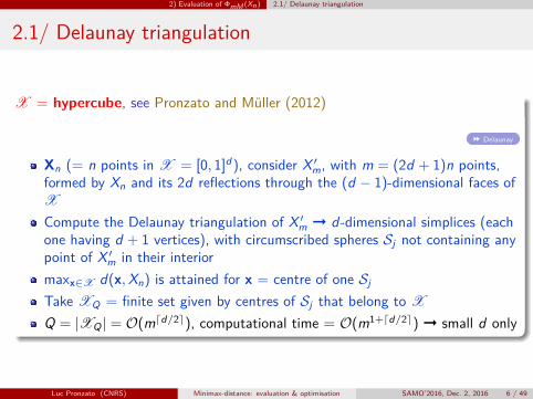
X = hypercube, see Pronzato and Müller (2012)
Delaunay
Xn (= n points in X = [0, 1]d), consider X ′m, with m = (2d + 1)n points,formed by Xn and its 2d reflections through the (d − 1)-dimensional faces ofX
Compute the Delaunay triangulation of X ′m Þ d-dimensional simplices (eachone having d + 1 vertices), with circumscribed spheres Sj not containing anypoint of X ′m in their interiormaxx∈X d(x,Xn) is attained for x = centre of one Sj
Take XQ = finite set given by centres of Sj that belong to X
Q = |XQ | = O(mdd/2e), computational time = O(m1+dd/2e) Þ small d only
Luc Pronzato (CNRS) Minimax-distance: evaluation & optimisation SAMO’2016, Dec. 2, 2016 6 / 49
2) Evaluation of ΦmM (Xn) 2.1/ Delaunay triangulation
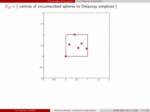
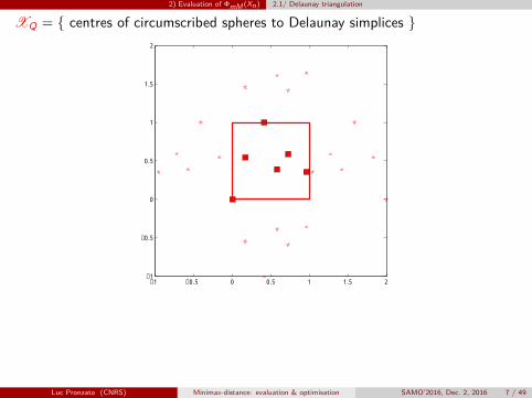
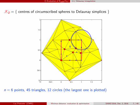
XQ = { centres of circumscribed spheres to Delaunay simplices }
−1 −0.5 0 0.5 1 1.5 2−1
−0.5
0
0.5
1
1.5
2
−1 −0.5 0 0.5 1 1.5 2−1
−0.5
0
0.5
1
1.5
2
n = 6 points, 45 triangles, 12 circles (the largest one is plotted)
Luc Pronzato (CNRS) Minimax-distance: evaluation & optimisation SAMO’2016, Dec. 2, 2016 7 / 49
2) Evaluation of ΦmM (Xn) 2.1/ Delaunay triangulation
XQ = { centres of circumscribed spheres to Delaunay simplices }
−1 −0.5 0 0.5 1 1.5 2−1
−0.5
0
0.5
1
1.5
2
n = 6 points, 45 triangles, 12 circles (the largest one is plotted)
Luc Pronzato (CNRS) Minimax-distance: evaluation & optimisation SAMO’2016, Dec. 2, 2016 7 / 49

2) Evaluation of ΦmM (Xn) 2.2/ Voronoï tessellation
2.2/ Voronoï tessellation
Voronoï
X = polytope in Rd , see Cortés and Bullo (2005, 2009)
Partition Rd into n cells Ci containing points closest to xi than to any othersite in Xn
Each Ci = convex polyhedron in Rd (some are open and infinite)X is a polytope of Rd ⇒ Ci ∩X = polytope Þ tessellation of X into nbounded convex polyhedramaxx∈X d(x,Xn) is attained when x is a vertex of one of these polyhedraTake XQ = collection of these verticesQ = O(ndd/2e) Þ small d onlyAvoid infinite cells by adding a few (at least d + 1) generators x′j out of X ,far enough from X to ensure that the corresponding cells do not intersect X
Luc Pronzato (CNRS) Minimax-distance: evaluation & optimisation SAMO’2016, Dec. 2, 2016 8 / 49

2) Evaluation of ΦmM (Xn) 2.2/ Voronoï tessellation
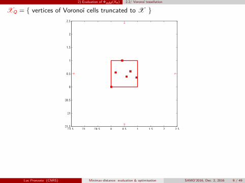
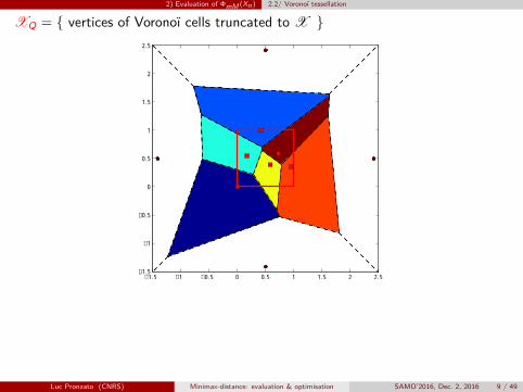
XQ = { vertices of Voronoï cells truncated to X }
−1.5 −1 −0.5 0 0.5 1 1.5 2 2.5−1.5
−1
−0.5
0
0.5
1
1.5
2
2.5
−1.5 −1 −0.5 0 0.5 1 1.5 2 2.5−1.5
−1
−0.5
0
0.5
1
1.5
2
2.5
n = 6 points, 6 cells, Q = 14 vertices x(k) tested for mini ‖x(k) − xi‖
Luc Pronzato (CNRS) Minimax-distance: evaluation & optimisation SAMO’2016, Dec. 2, 2016 9 / 49
2) Evaluation of ΦmM (Xn) 2.2/ Voronoï tessellation
XQ = { vertices of Voronoï cells truncated to X }
−1.5 −1 −0.5 0 0.5 1 1.5 2 2.5−1.5
−1
−0.5
0
0.5
1
1.5
2
2.5
−1.5 −1 −0.5 0 0.5 1 1.5 2 2.5−1.5
−1
−0.5
0
0.5
1
1.5
2
2.5
n = 6 points, 6 cells, Q = 14 vertices x(k) tested for mini ‖x(k) − xi‖
Luc Pronzato (CNRS) Minimax-distance: evaluation & optimisation SAMO’2016, Dec. 2, 2016 9 / 49

2) Evaluation of ΦmM (Xn) 2.2/ Voronoï tessellation
XQ = { vertices of Voronoï cells truncated to X }
−1.5 −1 −0.5 0 0.5 1 1.5 2 2.5−1.5
−1
−0.5
0
0.5
1
1.5
2
2.5
n = 6 points, 6 cells, Q = 14 vertices x(k) tested for mini ‖x(k) − xi‖
Luc Pronzato (CNRS) Minimax-distance: evaluation & optimisation SAMO’2016, Dec. 2, 2016 9 / 49

2) Evaluation of ΦmM (Xn) 2.3/ Estimation via MCMC
2.3/ Estimation via MCMC
2 ideas: extreme-value theory + multilevel splitting2.3a) Borrow results from extreme-value theory used in global optimisation(Zhigljavsky and Žilinskas, 2007, Chap. 2), (Zhigljavsky and Hamilton, 2010)
Q points x(j) i.i.d. in X , compute the Q distances dj = d(x(j),Xn),associated order statistics d1:Q ≥ d2:Q ≥ · · · ≥ dQ:Q
k fixed, 1 ≤ k ≤ Q (e.g., k = max{10, d}, Q � d), estimate ΦmM(Xn) by
Φ̂mM(Xn) = d1:Q + Ck(d1:Q − dk:Q)
where Ck = b1/(bk − b1) with bi = Γ(i + 1/d)/Γ(i).Also, the asymptotic confidence level of
Ik,δ =
[d1:Q , d1:Q +
d1:Q − dk:Q
(1− δ1/k)−1/d − 1
]tends to 1− δ for Q →∞Precise estimation only for very large Q à 2nd idea
Luc Pronzato (CNRS) Minimax-distance: evaluation & optimisation SAMO’2016, Dec. 2, 2016 10 / 49
2) Evaluation of ΦmM (Xn) 2.3/ Estimation via MCMC
2.3/ Estimation via MCMC
2 ideas: extreme-value theory + multilevel splitting2.3a) Borrow results from extreme-value theory used in global optimisation(Zhigljavsky and Žilinskas, 2007, Chap. 2), (Zhigljavsky and Hamilton, 2010)
Q points x(j) i.i.d. in X , compute the Q distances dj = d(x(j),Xn),associated order statistics d1:Q ≥ d2:Q ≥ · · · ≥ dQ:Q
k fixed, 1 ≤ k ≤ Q (e.g., k = max{10, d}, Q � d), estimate ΦmM(Xn) by
Φ̂mM(Xn) = d1:Q + Ck(d1:Q − dk:Q)
where Ck = b1/(bk − b1) with bi = Γ(i + 1/d)/Γ(i).Also, the asymptotic confidence level of
Ik,δ =
[d1:Q , d1:Q +
d1:Q − dk:Q
(1− δ1/k)−1/d − 1
]tends to 1− δ for Q →∞
Precise estimation only for very large Q à 2nd idea
Luc Pronzato (CNRS) Minimax-distance: evaluation & optimisation SAMO’2016, Dec. 2, 2016 10 / 49

2) Evaluation of ΦmM (Xn) 2.3/ Estimation via MCMC
2.3/ Estimation via MCMC
2 ideas: extreme-value theory + multilevel splitting2.3a) Borrow results from extreme-value theory used in global optimisation(Zhigljavsky and Žilinskas, 2007, Chap. 2), (Zhigljavsky and Hamilton, 2010)
Q points x(j) i.i.d. in X , compute the Q distances dj = d(x(j),Xn),associated order statistics d1:Q ≥ d2:Q ≥ · · · ≥ dQ:Q
k fixed, 1 ≤ k ≤ Q (e.g., k = max{10, d}, Q � d), estimate ΦmM(Xn) by
Φ̂mM(Xn) = d1:Q + Ck(d1:Q − dk:Q)
where Ck = b1/(bk − b1) with bi = Γ(i + 1/d)/Γ(i).Also, the asymptotic confidence level of
Ik,δ =
[d1:Q , d1:Q +
d1:Q − dk:Q
(1− δ1/k)−1/d − 1
]tends to 1− δ for Q →∞Precise estimation only for very large Q à 2nd ideaLuc Pronzato (CNRS) Minimax-distance: evaluation & optimisation SAMO’2016, Dec. 2, 2016 10 / 49

2) Evaluation of ΦmM (Xn) 2.3/ Estimation via MCMC
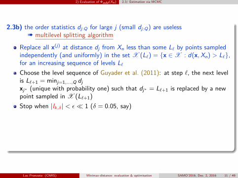
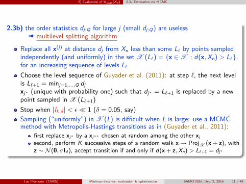
2.3b) the order statistics dj:Q for large j (small dj:Q) are uselessà multilevel splitting algorithm
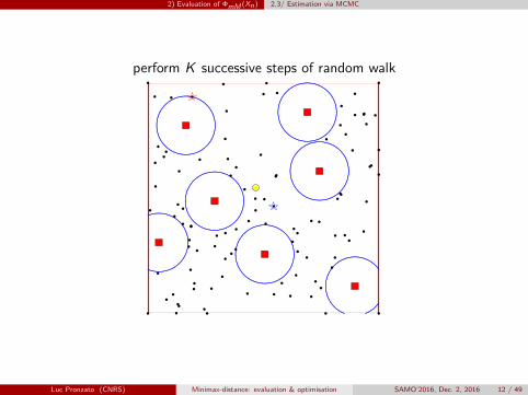
Replace all x(j) at distance dj from Xn less than some L` by points sampledindependently (and uniformly) in the set X (L`) = {x ∈X : d(x,Xn) > L`},for an increasing sequence of levels L`Choose the level sequence of Guyader et al. (2011): at step `, the next levelis L`+1 = minj=1,...,Q djxj∗ (unique with probability one) such that dj∗ = L`+1 is replaced by a newpoint sampled in X (L`+1)
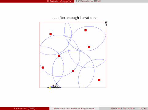
Stop when |Ik,δ| < ε� 1 (δ = 0.05, say)Sampling (“uniformly”) in X (L) is difficult when L is large: use a MCMCmethod with Metropolis-Hastings transitions as in (Guyader et al., 2011):
first replace xj∗ by a xj∗∗ chosen at random among the other xjsecond, perform K successive steps of a random walk x→ ProjX (x+ z), withz ∼ N (0, σId), accept transition if and only if d(x+ z,Xn) > L`+1 = dj∗
Luc Pronzato (CNRS) Minimax-distance: evaluation & optimisation SAMO’2016, Dec. 2, 2016 11 / 49
2) Evaluation of ΦmM (Xn) 2.3/ Estimation via MCMC
2.3b) the order statistics dj:Q for large j (small dj:Q) are uselessà multilevel splitting algorithm
Replace all x(j) at distance dj from Xn less than some L` by points sampledindependently (and uniformly) in the set X (L`) = {x ∈X : d(x,Xn) > L`},for an increasing sequence of levels L`
Choose the level sequence of Guyader et al. (2011): at step `, the next levelis L`+1 = minj=1,...,Q djxj∗ (unique with probability one) such that dj∗ = L`+1 is replaced by a newpoint sampled in X (L`+1)
Stop when |Ik,δ| < ε� 1 (δ = 0.05, say)Sampling (“uniformly”) in X (L) is difficult when L is large: use a MCMCmethod with Metropolis-Hastings transitions as in (Guyader et al., 2011):
first replace xj∗ by a xj∗∗ chosen at random among the other xjsecond, perform K successive steps of a random walk x→ ProjX (x+ z), withz ∼ N (0, σId), accept transition if and only if d(x+ z,Xn) > L`+1 = dj∗
Luc Pronzato (CNRS) Minimax-distance: evaluation & optimisation SAMO’2016, Dec. 2, 2016 11 / 49
2) Evaluation of ΦmM (Xn) 2.3/ Estimation via MCMC
2.3b) the order statistics dj:Q for large j (small dj:Q) are uselessà multilevel splitting algorithm
Replace all x(j) at distance dj from Xn less than some L` by points sampledindependently (and uniformly) in the set X (L`) = {x ∈X : d(x,Xn) > L`},for an increasing sequence of levels L`Choose the level sequence of Guyader et al. (2011): at step `, the next levelis L`+1 = minj=1,...,Q djxj∗ (unique with probability one) such that dj∗ = L`+1 is replaced by a newpoint sampled in X (L`+1)
Stop when |Ik,δ| < ε� 1 (δ = 0.05, say)
Sampling (“uniformly”) in X (L) is difficult when L is large: use a MCMCmethod with Metropolis-Hastings transitions as in (Guyader et al., 2011):
first replace xj∗ by a xj∗∗ chosen at random among the other xjsecond, perform K successive steps of a random walk x→ ProjX (x+ z), withz ∼ N (0, σId), accept transition if and only if d(x+ z,Xn) > L`+1 = dj∗
Luc Pronzato (CNRS) Minimax-distance: evaluation & optimisation SAMO’2016, Dec. 2, 2016 11 / 49
2) Evaluation of ΦmM (Xn) 2.3/ Estimation via MCMC
2.3b) the order statistics dj:Q for large j (small dj:Q) are uselessà multilevel splitting algorithm
Replace all x(j) at distance dj from Xn less than some L` by points sampledindependently (and uniformly) in the set X (L`) = {x ∈X : d(x,Xn) > L`},for an increasing sequence of levels L`Choose the level sequence of Guyader et al. (2011): at step `, the next levelis L`+1 = minj=1,...,Q djxj∗ (unique with probability one) such that dj∗ = L`+1 is replaced by a newpoint sampled in X (L`+1)
Stop when |Ik,δ| < ε� 1 (δ = 0.05, say)Sampling (“uniformly”) in X (L) is difficult when L is large: use a MCMCmethod with Metropolis-Hastings transitions as in (Guyader et al., 2011):
first replace xj∗ by a xj∗∗ chosen at random among the other xjsecond, perform K successive steps of a random walk x→ ProjX (x+ z), withz ∼ N (0, σId), accept transition if and only if d(x+ z,Xn) > L`+1 = dj∗
Luc Pronzato (CNRS) Minimax-distance: evaluation & optimisation SAMO’2016, Dec. 2, 2016 11 / 49
2) Evaluation of ΦmM (Xn) 2.3/ Estimation via MCMC
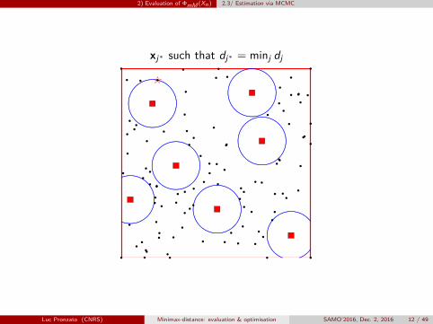
xj∗ such that dj∗ = minj dj
Luc Pronzato (CNRS) Minimax-distance: evaluation & optimisation SAMO’2016, Dec. 2, 2016 12 / 49
2) Evaluation of ΦmM (Xn) 2.3/ Estimation via MCMC
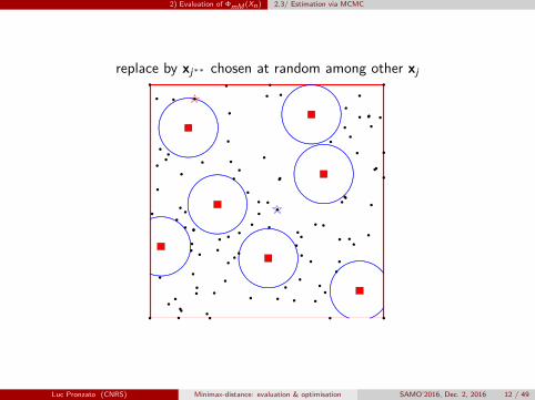
replace by xj∗∗ chosen at random among other xj
Luc Pronzato (CNRS) Minimax-distance: evaluation & optimisation SAMO’2016, Dec. 2, 2016 12 / 49
2) Evaluation of ΦmM (Xn) 2.3/ Estimation via MCMC
perform K successive steps of random walk
Luc Pronzato (CNRS) Minimax-distance: evaluation & optimisation SAMO’2016, Dec. 2, 2016 12 / 49
2) Evaluation of ΦmM (Xn) 2.3/ Estimation via MCMC
. . . after enough iterations
Luc Pronzato (CNRS) Minimax-distance: evaluation & optimisation SAMO’2016, Dec. 2, 2016 12 / 49
2) Evaluation of ΦmM (Xn) 2.3/ Estimation via MCMC
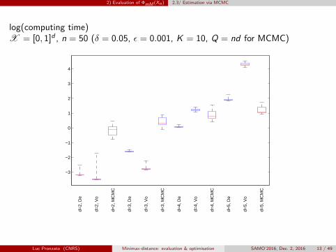
log(computing time)X = [0, 1]d , n = 50 (δ = 0.05, ε = 0.001, K = 10, Q = nd for MCMC)
−3
−2
−1
0
1
2
3
4
d=2,
De
d=2,
Vo
d=2,
MC
MC
d=3,
De
d=3,
Vo
d=3,
MC
MC
d=4,
De
d=4,
Vo
d=4,
MC
MC
d=5,
De
d=5,
Vo
d=5,
MC
MC
Luc Pronzato (CNRS) Minimax-distance: evaluation & optimisation SAMO’2016, Dec. 2, 2016 13 / 49

3) Optimisation of ΦmM (Xn)
3) Optimisation of ΦmM(Xn)
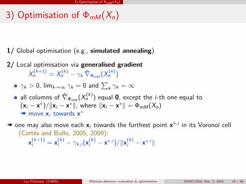
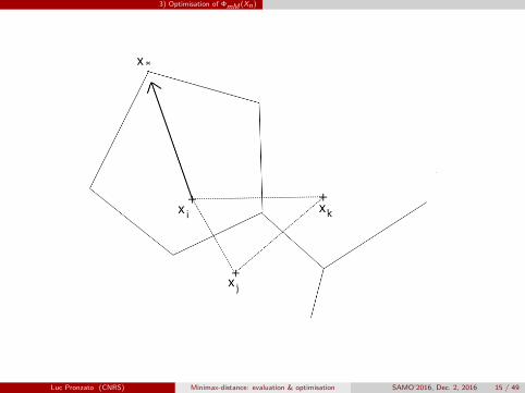
1/ Global optimisation (e.g., simulated annealing)
2/ Local optimisation via generalised gradientX (k+1)
n = X (k)n − γk ∇̃ΦmM (X (k)
n )
γk > 0, limk→∞ γk = 0 and∑
k γk =∞
all columns of ∇̃ΦmM (X (k)n ) equal 0, except the i-th one equal to
(xi − x∗)/‖xi − x∗‖, where ‖xi − x∗‖ = ΦmM(Xn)à move xi towards x∗
à one may also move each xi towards the furthest point x∗,i in its Voronoï cell(Cortés and Bullo, 2005, 2009):
x(k+1)i = x(k)
i − γk,i (x(k)i − x∗,i )/‖x(k)
i − x∗,i‖
Luc Pronzato (CNRS) Minimax-distance: evaluation & optimisation SAMO’2016, Dec. 2, 2016 14 / 49

3) Optimisation of ΦmM (Xn)
3) Optimisation of ΦmM(Xn)
1/ Global optimisation (e.g., simulated annealing)
2/ Local optimisation via generalised gradientX (k+1)
n = X (k)n − γk ∇̃ΦmM (X (k)
n )
γk > 0, limk→∞ γk = 0 and∑
k γk =∞
all columns of ∇̃ΦmM (X (k)n ) equal 0, except the i-th one equal to
(xi − x∗)/‖xi − x∗‖, where ‖xi − x∗‖ = ΦmM(Xn)à move xi towards x∗
à one may also move each xi towards the furthest point x∗,i in its Voronoï cell(Cortés and Bullo, 2005, 2009):
x(k+1)i = x(k)
i − γk,i (x(k)i − x∗,i )/‖x(k)
i − x∗,i‖
Luc Pronzato (CNRS) Minimax-distance: evaluation & optimisation SAMO’2016, Dec. 2, 2016 14 / 49
3) Optimisation of ΦmM (Xn)
Luc Pronzato (CNRS) Minimax-distance: evaluation & optimisation SAMO’2016, Dec. 2, 2016 15 / 49

3) Optimisation of ΦmM (Xn)
3/ kmeans and centroids
Tn = {Ci , i = 1, . . . , n} a tessellation of X , Xn a n-point design in XConsider the functional (Tn,Xn) −→ E2(Tn,Xn) =
∫X
(∑ni=1 wi (x) ‖x− xi‖2
)dx
where wi (x) = 1 if x ∈ Ci and 0 otherwise
Then, E2(Tn,Xn) =∑n
i=1∫Ci‖x− xi‖2 dx is minimised when
the Ci = Voronoï regions defined by the xi(Ô E2(Tn,Xn) =
∫X d2(x,Xn) dx)
simultaneously the xi = centroids of the Ci (centre of gravity),that is, xi = (
∫Cix dx)/vol(Ci ) (Du et al., 1999)
Þ such a Xn should thus perform reasonably well in terms of space-filling(Lekivetz and Jones, 2015)
Lloyd’s method (1982): fixed-point iterations forX (k)
n −→ X (k+1)n = T (X (k)
n ) = {T1(x(k)1 ), . . . ,Tn(x(k)
n )}with Ti (xi ) = (
∫Ci (Xn)
x dx)/vol[Ci (Xn)]
Use algorithmic geometry if d small enough; otherwise use a finite set XQ
Luc Pronzato (CNRS) Minimax-distance: evaluation & optimisation SAMO’2016, Dec. 2, 2016 16 / 49

3) Optimisation of ΦmM (Xn)
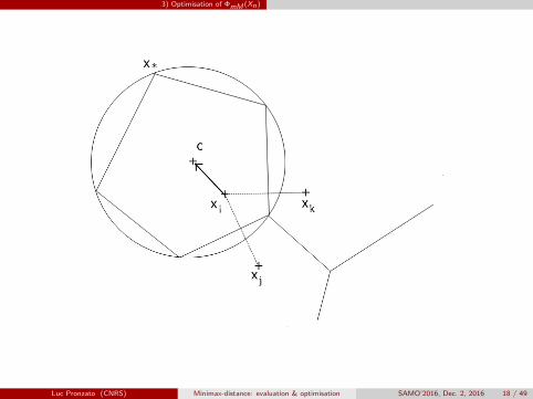
But minimax-optimal design is related to the construction of a centroidaltessellation for
Eq(Tn,Xn) =
∫X
( n∑i=1
wi (x) ‖x− xi‖q
)dx =
n∑i=1
∫Ci
‖x− xi‖q dx
with q →∞
Variant of Lloyd’s method:
0) Select X (1)n and ε� 1, set k = 1.
1) Compute the Voronoï tessellation {Ci , i = 1, . . . , n} of X (or XQ) based onX (k)
n
2) For i = 1, . . . , nä determine the smallest ball B(ci , ri ) enclosing Ci (= QP problem)ä replace xi by ci in X (k)
n
3) if ΦmM(X(k)n )− ΦmM(X(k+1)
n ) < ε, then stop; otherwise k ← k + 1, return tostep 1
Luc Pronzato (CNRS) Minimax-distance: evaluation & optimisation SAMO’2016, Dec. 2, 2016 17 / 49

3) Optimisation of ΦmM (Xn)
But minimax-optimal design is related to the construction of a centroidaltessellation for
Eq(Tn,Xn) =
∫X
( n∑i=1
wi (x) ‖x− xi‖q
)dx =
n∑i=1
∫Ci
‖x− xi‖q dx
with q →∞
Variant of Lloyd’s method:
0) Select X (1)n and ε� 1, set k = 1.
1) Compute the Voronoï tessellation {Ci , i = 1, . . . , n} of X (or XQ) based onX (k)
n
2) For i = 1, . . . , nä determine the smallest ball B(ci , ri ) enclosing Ci (= QP problem)ä replace xi by ci in X (k)
n
3) if ΦmM(X(k)n )− ΦmM(X(k+1)
n ) < ε, then stop; otherwise k ← k + 1, return tostep 1
Luc Pronzato (CNRS) Minimax-distance: evaluation & optimisation SAMO’2016, Dec. 2, 2016 17 / 49
3) Optimisation of ΦmM (Xn)
Luc Pronzato (CNRS) Minimax-distance: evaluation & optimisation SAMO’2016, Dec. 2, 2016 18 / 49

4) Nested designs
4) Nested designs (SIAM UQ, Lausanne, April 5–8 2016)
à obtain a high ΦmM-efficiency = Φ∗mM,n
ΦmM (Xn) for all Xn, nmin ≤ n ≤ nmax
(ΦmM-efficiency∈ (0, 1])
Luc Pronzato (CNRS) Minimax-distance: evaluation & optimisation SAMO’2016, Dec. 2, 2016 19 / 49

4) Nested designs 4.1/ Coffee-house design
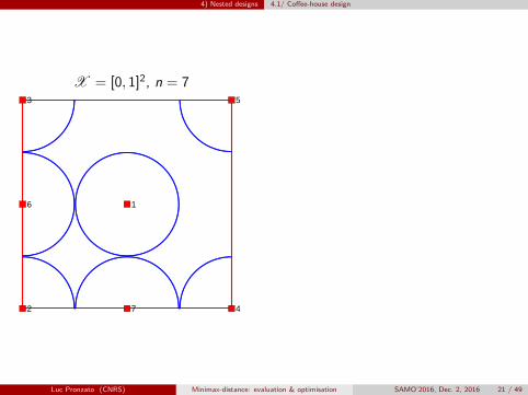
4.1/ Coffee-house design
x1 at the centre of X , then xn+1 furthest point from Xn for all n ≥ 1(called coffee-house design (Müller, 2007, Chap. 4))
Guarantees that ΦmM-efficiency = Φ∗mM,n
ΦmM (Xn) ≥12 for all n
[Indeed, by construction
ΦMm(Xn+1) , minxi 6=xj∈Xn+1
‖xi − xj‖ = d(xn+1,Xn) = ΦmM(Xn) ,
and ΦmM(X∗n ) ≥ 12 ΦMm(Xn+1) since one of the n balls B(x∗i ,ΦmM(X∗n )) must
contain 2 points from Xn+1 (Gonzalez, 1985)]
Luc Pronzato (CNRS) Minimax-distance: evaluation & optimisation SAMO’2016, Dec. 2, 2016 20 / 49

4) Nested designs 4.1/ Coffee-house design
4.1/ Coffee-house design
x1 at the centre of X , then xn+1 furthest point from Xn for all n ≥ 1(called coffee-house design (Müller, 2007, Chap. 4))
Guarantees that ΦmM-efficiency = Φ∗mM,n
ΦmM (Xn) ≥12 for all n
[Indeed, by construction
ΦMm(Xn+1) , minxi 6=xj∈Xn+1
‖xi − xj‖ = d(xn+1,Xn) = ΦmM(Xn) ,
and ΦmM(X∗n ) ≥ 12 ΦMm(Xn+1) since one of the n balls B(x∗i ,ΦmM(X∗n )) must
contain 2 points from Xn+1 (Gonzalez, 1985)]
Luc Pronzato (CNRS) Minimax-distance: evaluation & optimisation SAMO’2016, Dec. 2, 2016 20 / 49
4) Nested designs 4.1/ Coffee-house design
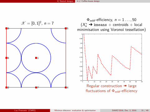
X = [0, 1]2, n = 7
1
2
3
4
5
6
7
ΦmM-efficiency, n = 1 . . . , 50(X∗n Ô kmeans + centroids + local
minimisation using Voronoï tessellation)
0 5 10 15 20 25 30 35 40 45 500.5
0.55
0.6
0.65
0.7
0.75
0.8
0.85
0.9
0.95
1
Regular construction à largefluctuations of ΦmM-efficiency
Luc Pronzato (CNRS) Minimax-distance: evaluation & optimisation SAMO’2016, Dec. 2, 2016 21 / 49
4) Nested designs 4.1/ Coffee-house design
X = [0, 1]2, n = 7
1
2
3
4
5
6
7
ΦmM-efficiency, n = 1 . . . , 50(X∗n Ô kmeans + centroids + local
minimisation using Voronoï tessellation)
0 5 10 15 20 25 30 35 40 45 500.5
0.55
0.6
0.65
0.7
0.75
0.8
0.85
0.9
0.95
1
Regular construction à largefluctuations of ΦmM-efficiency
Luc Pronzato (CNRS) Minimax-distance: evaluation & optimisation SAMO’2016, Dec. 2, 2016 21 / 49
4) Nested designs 4.2/ Submodularity and greedy algorithms
4.2/ Submodularity and greedy algorithms
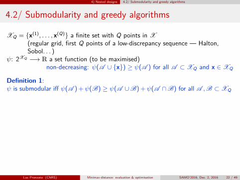
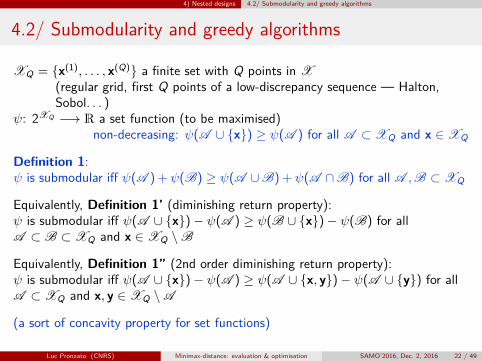
XQ = {x(1), . . . , x(Q)} a finite set with Q points in X(regular grid, first Q points of a low-discrepancy sequence — Halton,Sobol. . . )
ψ: 2XQ −→ R a set function (to be maximised)non-decreasing: ψ(A ∪ {x}) ≥ ψ(A ) for all A ⊂XQ and x ∈XQ
Definition 1:ψ is submodular iff ψ(A ) +ψ(B) ≥ ψ(A ∪B) +ψ(A ∩B) for all A ,B ⊂XQ
Equivalently, Definition 1’ (diminishing return property):ψ is submodular iff ψ(A ∪ {x})− ψ(A ) ≥ ψ(B ∪ {x})− ψ(B) for allA ⊂ B ⊂XQ and x ∈XQ \B
Equivalently, Definition 1” (2nd order diminishing return property):ψ is submodular iff ψ(A ∪ {x})− ψ(A ) ≥ ψ(A ∪ {x, y})− ψ(A ∪ {y}) for allA ⊂XQ and x, y ∈XQ \A
(a sort of concavity property for set functions)
Luc Pronzato (CNRS) Minimax-distance: evaluation & optimisation SAMO’2016, Dec. 2, 2016 22 / 49
4) Nested designs 4.2/ Submodularity and greedy algorithms
4.2/ Submodularity and greedy algorithms
XQ = {x(1), . . . , x(Q)} a finite set with Q points in X(regular grid, first Q points of a low-discrepancy sequence — Halton,Sobol. . . )
ψ: 2XQ −→ R a set function (to be maximised)non-decreasing: ψ(A ∪ {x}) ≥ ψ(A ) for all A ⊂XQ and x ∈XQ
Definition 1:ψ is submodular iff ψ(A ) +ψ(B) ≥ ψ(A ∪B) +ψ(A ∩B) for all A ,B ⊂XQ
Equivalently, Definition 1’ (diminishing return property):ψ is submodular iff ψ(A ∪ {x})− ψ(A ) ≥ ψ(B ∪ {x})− ψ(B) for allA ⊂ B ⊂XQ and x ∈XQ \B
Equivalently, Definition 1” (2nd order diminishing return property):ψ is submodular iff ψ(A ∪ {x})− ψ(A ) ≥ ψ(A ∪ {x, y})− ψ(A ∪ {y}) for allA ⊂XQ and x, y ∈XQ \A
(a sort of concavity property for set functions)
Luc Pronzato (CNRS) Minimax-distance: evaluation & optimisation SAMO’2016, Dec. 2, 2016 22 / 49

4) Nested designs 4.2/ Submodularity and greedy algorithms
Greedy Algorithm:1 set A = ∅2 while |A | < k
find x in XQ such that ψ(A ∪ {x}) is maximalA ← A ∪ {x}
3 end while4 return Ak = A
Denote ψ∗k = maxB⊂XQ , |B|≤k ψ(B)
Theorem (Nemhauser, Wolsey & Fisher, 1978): When ψ is non-decreasing andsubmodular, then for all k ∈ {1, . . . ,Q} the algorithm returns a set Ak such that
ψ(Ak)− ψ(∅)ψ∗k − ψ(∅)
≥ 1− (1− 1/k)k ≥ 1− 1/e > 0.6321
Bad news: we maximise −ΦmM which is non-decreasing but not submodularà no guaranteed efficiency for sequential optimisation
Luc Pronzato (CNRS) Minimax-distance: evaluation & optimisation SAMO’2016, Dec. 2, 2016 23 / 49

4) Nested designs 4.3/ Covering measure, c.d.f. and dispersion
4.3/ Covering measure, c.d.f. and dispersion
For any r ≥ 0, any Xn ∈X n, define the covering measure of Xn byψr (Xn) = vol{X ∩ [∪n
i=1B(xi , r)]} à non-decreasing and submodular
Maximising ψr (Xn) is equivalent to maximisingFXn (r) = ψr (Xn)/vol(X ) =
µL{X ∩[∪ni=1B(xi ,r)]}
µL(X )
which can be considered as a c.d.f., with FXn (r) ∈ [0, 1], increasing in r , andFXn (0) = 0, FXn (r) = 1 for any r ≥ ΦmM(Xn) = dispersion of Xn
Take any probability measure µ on X (e.g., with finite support XQ)à define FXn (r) = µ{X ∩ [∪n
i=1B(xi , r)]}as a function of r Ô forms a c.d.f.,as a function of Xn Ô non-decreasing and submodular
Luc Pronzato (CNRS) Minimax-distance: evaluation & optimisation SAMO’2016, Dec. 2, 2016 24 / 49

4) Nested designs 4.3/ Covering measure, c.d.f. and dispersion
Which r should we take in FXn (r)?A positive linear combination of non-decreasing submodular functions isnon-decreasing and submodular
à Consider Cb,B,q(Xn) =∫ B
b rq FXn (r) dr , for B > b ≥ 0, q > 0Ô We have guaranteed efficiency bounds when maximising with a greedyalgorithm
Justification:
C0,B,q(Xn) = Bq+1
q+1 FXn (B)− 1q+1
∫ B0 rq+1 FXn (dr)
Take any B ≥ ΦmM(Xn) Ô FXn (B) = 1Maximising C0,B,q(Xn) for B large enough ⇔ minimising
∫ B0 rq+1 FXn (dr)
⇔ minimising[∫ B
0 rq+1 FXn (dr)]1/(q+1)
and[∫ B
0 rq+1 FXn (dr)]1/(q+1)
→ ΦmM(Xn) as q →∞
Luc Pronzato (CNRS) Minimax-distance: evaluation & optimisation SAMO’2016, Dec. 2, 2016 25 / 49

4) Nested designs 4.4/ Implementation
4.4/ Implementation
Take XQ = {x(1), . . . , x(Q)} ⊂X Q , µ = 1Q∑Q
j=1 δx(j)
For any design Xn = {x1, . . . , xn} ⊂X n, denoterj = d(x(j),Xn) = mini=1,...,n ‖x(j) − xi‖ andrk:Q the k-th order statistic of the ri : r1:Q ≤ r2:Q ≤ · · · ≤ rQ:Qr ′k:Q = min{max{rk:Q , b},B} for all k = 1, . . . ,Q and r ′Q+1:Q = B
Then Cb,B,q(Xn) = 1Q(q+1)
∑Qk=1 k[r ′k+1:Q
q+1 − r ′k:Qq+1
]
Note: when Xn ⊂XQ , the inter-distances ‖x(i) − x(j)‖ will be computed only once
Luc Pronzato (CNRS) Minimax-distance: evaluation & optimisation SAMO’2016, Dec. 2, 2016 26 / 49

4) Nested designs 4.4/ Implementation
Remark:
When b = 0 and B ≥ ΦmM(Xn), Cb,B,q(Xn) = Bq+1
q+1 −1
nQ(q+1)
∑Qk=1
∑ni=1 γk,i
with γk,i = dq+1(x(k),Xn) = mini=1,...,n ‖x(k) − xi‖q+1 for all i = 1, . . . , nÔ the maximisation of C0,B,q(Xn) corresponds to a “facility location problem”with assignment costs γk,i (Minoux, 1977):
minimise 1nQ
Q∑k=1
n∑i=1
γk,i
. . . but solving such a facility location problem with assignment costsγk,i = [min{d(x(k),Xn),B}]q+1 does not work if the truncation at B too small
d = 2, X = [0, 1]2, XQ= regular gridwith 33× 33 points
b = 0, B =√2/2 à all xi coincide with
one corner of X
Luc Pronzato (CNRS) Minimax-distance: evaluation & optimisation SAMO’2016, Dec. 2, 2016 27 / 49

4) Nested designs 4.4/ Implementation
Ô sequential maximisation of Cb,B,q(Xn) = 1Q(q+1)
∑Qk=1 k[r ′k+1:Q
q+1 − r ′k:Qq+1
]
with r ′k:Q ∈ [b,B] for all k
We shall need bounds R∗n and R∗n on Φ∗mM,n = ΦmM(X∗n )
Lower bound R∗n ≤ Φ∗mM,n: sphere-covering problem
The n balls B(xi ,Φ∗mM,n) cover X ⇒ nVd (Φ∗mM)d ≥ vol(X ) (= 1), with
Vd = vol[B(0, 1)] = πd/2/Γ(d/2 + 1)
R∗n = (nVd )−1/d ≤ Φ∗mM,n
Luc Pronzato (CNRS) Minimax-distance: evaluation & optimisation SAMO’2016, Dec. 2, 2016 28 / 49

4) Nested designs 4.4/ Implementation
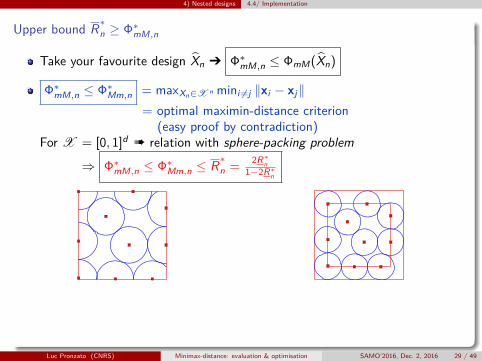
Upper bound R∗n ≥ Φ∗mM,n
Take your favourite design X̂n Ô Φ∗mM,n ≤ ΦmM(X̂n)
Φ∗mM,n ≤ Φ∗Mm,n = maxXn∈X n mini 6=j ‖xi − xj‖= optimal maximin-distance criterion
(easy proof by contradiction)
For X = [0, 1]d à relation with sphere-packing problem
⇒ Φ∗mM,n ≤ Φ∗Mm,n ≤ R∗n =2R∗
n1−2R∗
n
This requires n > d2d/Vde (to have R∗n < 12 )
For n ≤⌈
1Vd
(12
√d
2+√
d
)−d⌉use the trivial bound Φ∗mM,n ≤ R∗n =
√d/2
Luc Pronzato (CNRS) Minimax-distance: evaluation & optimisation SAMO’2016, Dec. 2, 2016 29 / 49

4) Nested designs 4.4/ Implementation
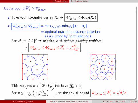
Upper bound R∗n ≥ Φ∗mM,n
Take your favourite design X̂n Ô Φ∗mM,n ≤ ΦmM(X̂n)
Φ∗mM,n ≤ Φ∗Mm,n = maxXn∈X n mini 6=j ‖xi − xj‖= optimal maximin-distance criterion
(easy proof by contradiction)
For X = [0, 1]d à relation with sphere-packing problem
⇒ Φ∗mM,n ≤ Φ∗Mm,n ≤ R∗n =2R∗
n1−2R∗
n
This requires n > d2d/Vde (to have R∗n < 12 )
For n ≤⌈
1Vd
(12
√d
2+√
d
)−d⌉use the trivial bound Φ∗mM,n ≤ R∗n =
√d/2
Luc Pronzato (CNRS) Minimax-distance: evaluation & optimisation SAMO’2016, Dec. 2, 2016 29 / 49
4) Nested designs 4.4/ Implementation
Upper bound R∗n ≥ Φ∗mM,n
Take your favourite design X̂n Ô Φ∗mM,n ≤ ΦmM(X̂n)
Φ∗mM,n ≤ Φ∗Mm,n = maxXn∈X n mini 6=j ‖xi − xj‖= optimal maximin-distance criterion
(easy proof by contradiction)For X = [0, 1]d à relation with sphere-packing problem
⇒ Φ∗mM,n ≤ Φ∗Mm,n ≤ R∗n =2R∗
n1−2R∗
n
This requires n > d2d/Vde (to have R∗n < 12 )
For n ≤⌈
1Vd
(12
√d
2+√
d
)−d⌉use the trivial bound Φ∗mM,n ≤ R∗n =
√d/2
Luc Pronzato (CNRS) Minimax-distance: evaluation & optimisation SAMO’2016, Dec. 2, 2016 29 / 49

4) Nested designs 4.4/ Implementation
Choices of b and B
¬ B large Ô the construction is too regular
d = 2, X = [0, 1]2, XQ= regular gridwith 33× 33 points
b = 0, B =√2 à ΦmM-efficiency will
periodically reach low values
We want a high ΦmM-efficiency for nmin ≤ n ≤ nmaxÔ set B & upper bound R∗nmax
on Φ∗mM,nmaxB & lower bound R∗nmin
on Φ∗mM,nmin
Ô take B = max{R∗nmax,R∗nmin
} (not critical)
Luc Pronzato (CNRS) Minimax-distance: evaluation & optimisation SAMO’2016, Dec. 2, 2016 30 / 49
4) Nested designs 4.4/ Implementation
d = 2, X = [0, 1]2, XQ= regular gridwith 33× 33 points
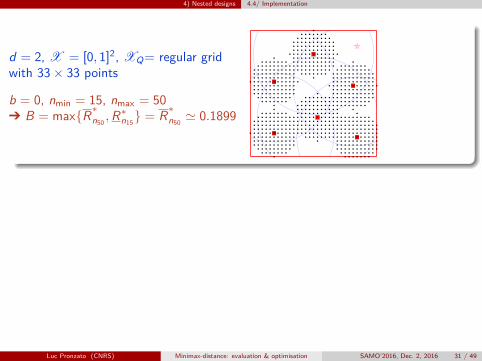
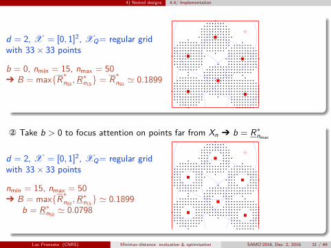
b = 0, nmin = 15, nmax = 50Ô B = max{R∗n50
,R∗n15} = R∗n50
' 0.1899
Take b > 0 to focus attention on points far from Xn Ô b = R∗nmax
d = 2, X = [0, 1]2, XQ= regular gridwith 33× 33 points
nmin = 15, nmax = 50Ô B = max{R∗n50
,R∗n15} ' 0.1899
b = R∗n50' 0.0798
Luc Pronzato (CNRS) Minimax-distance: evaluation & optimisation SAMO’2016, Dec. 2, 2016 31 / 49
4) Nested designs 4.4/ Implementation
d = 2, X = [0, 1]2, XQ= regular gridwith 33× 33 points
b = 0, nmin = 15, nmax = 50Ô B = max{R∗n50
,R∗n15} = R∗n50
' 0.1899
Take b > 0 to focus attention on points far from Xn Ô b = R∗nmax
d = 2, X = [0, 1]2, XQ= regular gridwith 33× 33 points
nmin = 15, nmax = 50Ô B = max{R∗n50
,R∗n15} ' 0.1899
b = R∗n50' 0.0798
Luc Pronzato (CNRS) Minimax-distance: evaluation & optimisation SAMO’2016, Dec. 2, 2016 31 / 49

4) Nested designs 4.4/ Implementation
Choice of qNot crucial, in theory should be large, but q = 2 seems ok
Luc Pronzato (CNRS) Minimax-distance: evaluation & optimisation SAMO’2016, Dec. 2, 2016 32 / 49

4) Nested designs 4.5/ Illustration (small d)
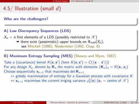
4.5/ Illustration (small d)
Who are the challengers?
A) Low Discrepancy Sequences (LDS)Xn = n first elements of a LDS (possibly restricted to X )
à there exist (pessimistic) upper bounds on ΦmM(Xn),see Mitchell (1990), Niederreiter (1992, Chap. 6)
B) Maximum Entropy Sampling (MES) (Shewry and Wynn, 1987)Take a (covariance) kernel K (x, x′) (here K (x, x′) = C(‖x− x′‖))For any design Xn, denote by Kn the matrix with elements {Kn}ij = K (xi , xj)Choose sequentially xk+1 that maximises detKn+1⇔ greedy maximisation of entropy for a Gaussian process with covariance K⇔ xk+1 maximises the current kriging variance ρ2k(x) (x1 = centre of X )
If C(t) is decreasing, a maximin optimal design that maximises mini 6=j ‖xi − xj‖ isasymptotically MES optimum for C s as s →∞ (Johnson et al., 1990)
Ô many points on (near) the boundary of X
Luc Pronzato (CNRS) Minimax-distance: evaluation & optimisation SAMO’2016, Dec. 2, 2016 33 / 49
4) Nested designs 4.5/ Illustration (small d)
4.5/ Illustration (small d)
Who are the challengers?
A) Low Discrepancy Sequences (LDS)Xn = n first elements of a LDS (possibly restricted to X )
à there exist (pessimistic) upper bounds on ΦmM(Xn),see Mitchell (1990), Niederreiter (1992, Chap. 6)
B) Maximum Entropy Sampling (MES) (Shewry and Wynn, 1987)Take a (covariance) kernel K (x, x′) (here K (x, x′) = C(‖x− x′‖))For any design Xn, denote by Kn the matrix with elements {Kn}ij = K (xi , xj)Choose sequentially xk+1 that maximises detKn+1⇔ greedy maximisation of entropy for a Gaussian process with covariance K⇔ xk+1 maximises the current kriging variance ρ2k(x) (x1 = centre of X )
If C(t) is decreasing, a maximin optimal design that maximises mini 6=j ‖xi − xj‖ isasymptotically MES optimum for C s as s →∞ (Johnson et al., 1990)
Ô many points on (near) the boundary of X
Luc Pronzato (CNRS) Minimax-distance: evaluation & optimisation SAMO’2016, Dec. 2, 2016 33 / 49

4) Nested designs 4.5/ Illustration (small d)
4.5/ Illustration (small d)
Who are the challengers?
A) Low Discrepancy Sequences (LDS)Xn = n first elements of a LDS (possibly restricted to X )
à there exist (pessimistic) upper bounds on ΦmM(Xn),see Mitchell (1990), Niederreiter (1992, Chap. 6)
B) Maximum Entropy Sampling (MES) (Shewry and Wynn, 1987)Take a (covariance) kernel K (x, x′) (here K (x, x′) = C(‖x− x′‖))For any design Xn, denote by Kn the matrix with elements {Kn}ij = K (xi , xj)Choose sequentially xk+1 that maximises detKn+1⇔ greedy maximisation of entropy for a Gaussian process with covariance K⇔ xk+1 maximises the current kriging variance ρ2k(x) (x1 = centre of X )
If C(t) is decreasing, a maximin optimal design that maximises mini 6=j ‖xi − xj‖ isasymptotically MES optimum for C s as s →∞ (Johnson et al., 1990)
Ô many points on (near) the boundary of XLuc Pronzato (CNRS) Minimax-distance: evaluation & optimisation SAMO’2016, Dec. 2, 2016 33 / 49

4) Nested designs 4.5/ Illustration (small d)
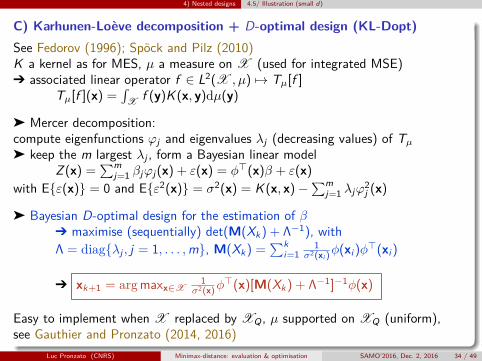
C) Karhunen-Loève decomposition + D-optimal design (KL-Dopt)See Fedorov (1996); Spöck and Pilz (2010)K a kernel as for MES, µ a measure on X (used for integrated MSE)Ô associated linear operator f ∈ L2(X , µ) 7→ Tµ[f ]
Tµ[f ](x) =∫
X f (y)K (x, y)dµ(y)
ä Mercer decomposition:compute eigenfunctions ϕj and eigenvalues λj (decreasing values) of Tµä keep the m largest λj , form a Bayesian linear model
Z (x) =∑m
j=1 βjϕj(x) + ε(x) = φ>(x)β + ε(x)
with E{ε(x)} = 0 and E{ε2(x)} = σ2(x) = K (x, x)−∑m
j=1 λjϕ2j (x)
ä Bayesian D-optimal design for the estimation of βÔ maximise (sequentially) det(M(Xk) + Λ−1), withΛ = diag{λj , j = 1, . . . ,m}, M(Xk) =
∑ki=1
1σ2(xi )
φ(xi )φ>(xi )
Ô xk+1 = argmaxx∈X1
σ2(x)φ>(x)[M(Xk) + Λ−1]−1φ(x)
Easy to implement when X replaced by XQ , µ supported on XQ (uniform),see Gauthier and Pronzato (2014, 2016)
Luc Pronzato (CNRS) Minimax-distance: evaluation & optimisation SAMO’2016, Dec. 2, 2016 34 / 49
4) Nested designs 4.5/ Illustration (small d)
C) Karhunen-Loève decomposition + D-optimal design (KL-Dopt)See Fedorov (1996); Spöck and Pilz (2010)K a kernel as for MES, µ a measure on X (used for integrated MSE)Ô associated linear operator f ∈ L2(X , µ) 7→ Tµ[f ]
Tµ[f ](x) =∫
X f (y)K (x, y)dµ(y)
ä Mercer decomposition:compute eigenfunctions ϕj and eigenvalues λj (decreasing values) of Tµä keep the m largest λj , form a Bayesian linear model
Z (x) =∑m
j=1 βjϕj(x) + ε(x) = φ>(x)β + ε(x)
with E{ε(x)} = 0 and E{ε2(x)} = σ2(x) = K (x, x)−∑m
j=1 λjϕ2j (x)
ä Bayesian D-optimal design for the estimation of βÔ maximise (sequentially) det(M(Xk) + Λ−1), withΛ = diag{λj , j = 1, . . . ,m}, M(Xk) =
∑ki=1
1σ2(xi )
φ(xi )φ>(xi )
Ô xk+1 = argmaxx∈X1
σ2(x)φ>(x)[M(Xk) + Λ−1]−1φ(x)
Easy to implement when X replaced by XQ , µ supported on XQ (uniform),see Gauthier and Pronzato (2014, 2016)
Luc Pronzato (CNRS) Minimax-distance: evaluation & optimisation SAMO’2016, Dec. 2, 2016 34 / 49

4) Nested designs 4.5/ Illustration (small d)
To facilitate calculations: take K = tensorised form of a uni-dimensional kernel,for instance, K (x, x′) = exp(−θ ‖x− x′‖2)Ô ϕj and λj = product of eigenfunctions ϕ`,1 and eigenvalues λ`,1
in the uni-dimensional decomposition (with degeneracy of λj ≤ d!)Ô organise the combination of ϕ`,1 and λ`,1 to keep m largest λj
Since n ≤ nmax, m = dim(β) should not be much larger than nmaxÔ Take the smallest m ≥ nmax such that λm+1 < λm
Luc Pronzato (CNRS) Minimax-distance: evaluation & optimisation SAMO’2016, Dec. 2, 2016 35 / 49
4) Nested designs 4.5/ Illustration (small d)
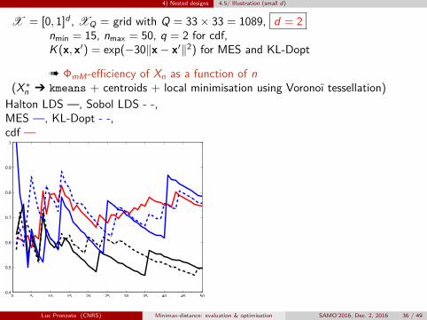
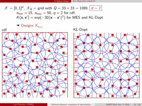
X = [0, 1]d , XQ = grid with Q = 33× 33 = 1089, d = 2nmin = 15, nmax = 50, q = 2 for cdf,K (x, x′) = exp(−30‖x− x′‖2) for MES and KL-Dopt
à ΦmM-efficiency of Xn as a function of n(X∗n Ô kmeans + centroids + local minimisation using Voronoï tessellation)
Halton LDS —, Sobol LDS - -,MES —, KL-Dopt - -,cdf —
0 5 10 15 20 25 30 35 40 45 500.4
0.5
0.6
0.7
0.8
0.9
1
Permutations: exchange xk with xk+1when ΦmM improvesstarting from k = 1, repeat several times
0 5 10 15 20 25 30 35 40 45 500.4
0.5
0.6
0.7
0.8
0.9
1
Luc Pronzato (CNRS) Minimax-distance: evaluation & optimisation SAMO’2016, Dec. 2, 2016 36 / 49
4) Nested designs 4.5/ Illustration (small d)
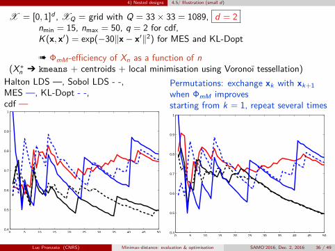
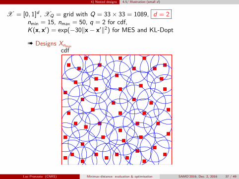
X = [0, 1]d , XQ = grid with Q = 33× 33 = 1089, d = 2nmin = 15, nmax = 50, q = 2 for cdf,K (x, x′) = exp(−30‖x− x′‖2) for MES and KL-Dopt
à Designs Xnmaxcdf
Luc Pronzato (CNRS) Minimax-distance: evaluation & optimisation SAMO’2016, Dec. 2, 2016 37 / 49
4) Nested designs 4.5/ Illustration (small d)
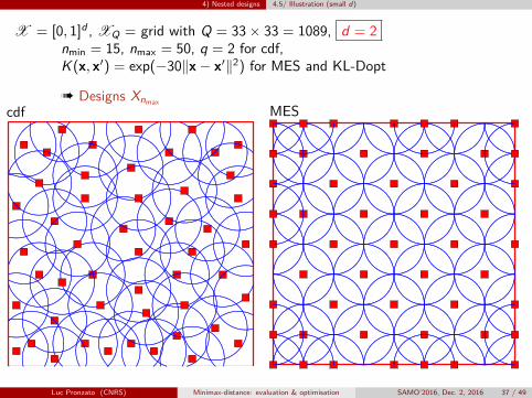
X = [0, 1]d , XQ = grid with Q = 33× 33 = 1089, d = 2nmin = 15, nmax = 50, q = 2 for cdf,K (x, x′) = exp(−30‖x− x′‖2) for MES and KL-Dopt
à Designs Xnmaxcdf MES
Luc Pronzato (CNRS) Minimax-distance: evaluation & optimisation SAMO’2016, Dec. 2, 2016 37 / 49
4) Nested designs 4.5/ Illustration (small d)
X = [0, 1]d , XQ = grid with Q = 33× 33 = 1089, d = 2nmin = 15, nmax = 50, q = 2 for cdf,K (x, x′) = exp(−30‖x− x′‖2) for MES and KL-Dopt
à Designs Xnmax
cdf KL-Dopt
Luc Pronzato (CNRS) Minimax-distance: evaluation & optimisation SAMO’2016, Dec. 2, 2016 37 / 49
4) Nested designs 4.5/ Illustration (small d)
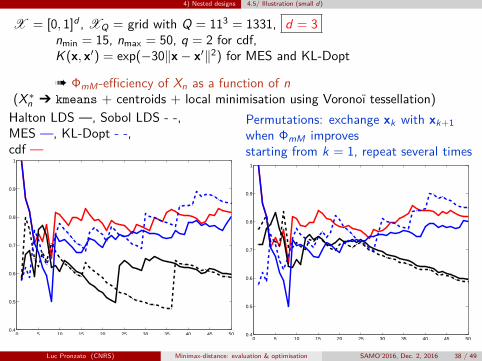
X = [0, 1]d , XQ = grid with Q = 113 = 1331, d = 3nmin = 15, nmax = 50, q = 2 for cdf,K (x, x′) = exp(−30‖x− x′‖2) for MES and KL-Dopt
à ΦmM-efficiency of Xn as a function of n(X∗n Ô kmeans + centroids + local minimisation using Voronoï tessellation)Halton LDS —, Sobol LDS - -,MES —, KL-Dopt - -,cdf —
0 5 10 15 20 25 30 35 40 45 500.4
0.5
0.6
0.7
0.8
0.9
1
Permutations: exchange xk with xk+1when ΦmM improvesstarting from k = 1, repeat several times
0 5 10 15 20 25 30 35 40 45 500.4
0.5
0.6
0.7
0.8
0.9
1
Luc Pronzato (CNRS) Minimax-distance: evaluation & optimisation SAMO’2016, Dec. 2, 2016 38 / 49

4) Nested designs 4.6/ d > 3
4.6/ d > 3
For large d (d > 3, say), we cannot use a regular grid XQ
If d not too large, XQ = first Q points of a LDS
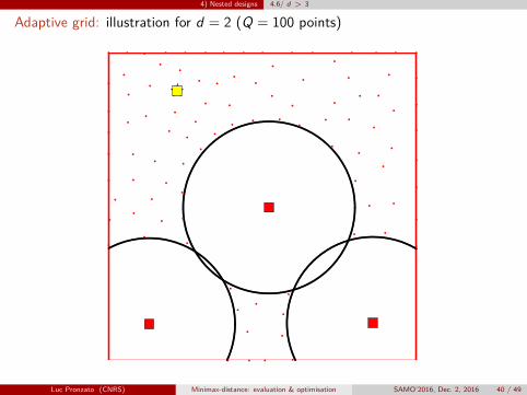
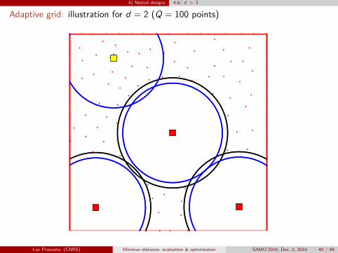
When X = [0, 1]d , XQ = { some interesting points in X }, e.g.,{centre of X } ∪ {2d vertices} ∪ {some points on the boundary of X }Adaptive grid: modify XQ as k increases by a MCMC technique
1 Initialise XQ,0 with Q points well spread in X , compute x1, set k = 12 Consider all balls B(xi ,R∗k+1) as forbidden
Ô obtain XQ,k by repositioning all points of XQ,k−1 in X \ [∪ki=1B(xi ,R∗k+1)],
3 Compute xk+1, k + 1← k, return to step 2
At step 1: A few (25, say) iterations of Metropolis-Hasting (simulated-annealing) tominimise energy EQ ∝
∑i<j
1‖xi−xj‖d+1
At step 2: Each x(j) in the forbidden region ∪ki=1B(xi ,R∗k+1) is first moved to the
admissible part (substitution by a randomly selected admissible x(`) + a few steps ofrandom walk), then a few iterations of simulated annealing again to minimise energy
Q = max{d × nmax, 100} seems to be enough (for cdf, MES,KL-Dopt)
Luc Pronzato (CNRS) Minimax-distance: evaluation & optimisation SAMO’2016, Dec. 2, 2016 39 / 49

4) Nested designs 4.6/ d > 3
4.6/ d > 3
For large d (d > 3, say), we cannot use a regular grid XQ
If d not too large, XQ = first Q points of a LDSWhen X = [0, 1]d , XQ = { some interesting points in X }, e.g.,{centre of X } ∪ {2d vertices} ∪ {some points on the boundary of X }
Adaptive grid: modify XQ as k increases by a MCMC technique1 Initialise XQ,0 with Q points well spread in X , compute x1, set k = 12 Consider all balls B(xi ,R∗k+1) as forbidden
Ô obtain XQ,k by repositioning all points of XQ,k−1 in X \ [∪ki=1B(xi ,R∗k+1)],
3 Compute xk+1, k + 1← k, return to step 2
At step 1: A few (25, say) iterations of Metropolis-Hasting (simulated-annealing) tominimise energy EQ ∝
∑i<j
1‖xi−xj‖d+1
At step 2: Each x(j) in the forbidden region ∪ki=1B(xi ,R∗k+1) is first moved to the
admissible part (substitution by a randomly selected admissible x(`) + a few steps ofrandom walk), then a few iterations of simulated annealing again to minimise energy
Q = max{d × nmax, 100} seems to be enough (for cdf, MES,KL-Dopt)
Luc Pronzato (CNRS) Minimax-distance: evaluation & optimisation SAMO’2016, Dec. 2, 2016 39 / 49

4) Nested designs 4.6/ d > 3
4.6/ d > 3
For large d (d > 3, say), we cannot use a regular grid XQ
If d not too large, XQ = first Q points of a LDSWhen X = [0, 1]d , XQ = { some interesting points in X }, e.g.,{centre of X } ∪ {2d vertices} ∪ {some points on the boundary of X }Adaptive grid: modify XQ as k increases by a MCMC technique
1 Initialise XQ,0 with Q points well spread in X , compute x1, set k = 12 Consider all balls B(xi ,R∗k+1) as forbidden
Ô obtain XQ,k by repositioning all points of XQ,k−1 in X \ [∪ki=1B(xi ,R∗k+1)],
3 Compute xk+1, k + 1← k, return to step 2
At step 1: A few (25, say) iterations of Metropolis-Hasting (simulated-annealing) tominimise energy EQ ∝
∑i<j
1‖xi−xj‖d+1
At step 2: Each x(j) in the forbidden region ∪ki=1B(xi ,R∗k+1) is first moved to the
admissible part (substitution by a randomly selected admissible x(`) + a few steps ofrandom walk), then a few iterations of simulated annealing again to minimise energy
Q = max{d × nmax, 100} seems to be enough (for cdf, MES,KL-Dopt)
Luc Pronzato (CNRS) Minimax-distance: evaluation & optimisation SAMO’2016, Dec. 2, 2016 39 / 49

4) Nested designs 4.6/ d > 3
4.6/ d > 3
For large d (d > 3, say), we cannot use a regular grid XQ
If d not too large, XQ = first Q points of a LDSWhen X = [0, 1]d , XQ = { some interesting points in X }, e.g.,{centre of X } ∪ {2d vertices} ∪ {some points on the boundary of X }Adaptive grid: modify XQ as k increases by a MCMC technique
1 Initialise XQ,0 with Q points well spread in X , compute x1, set k = 12 Consider all balls B(xi ,R∗k+1) as forbidden
Ô obtain XQ,k by repositioning all points of XQ,k−1 in X \ [∪ki=1B(xi ,R∗k+1)],
3 Compute xk+1, k + 1← k, return to step 2At step 1: A few (25, say) iterations of Metropolis-Hasting (simulated-annealing) tominimise energy EQ ∝
∑i<j
1‖xi−xj‖d+1
At step 2: Each x(j) in the forbidden region ∪ki=1B(xi ,R∗k+1) is first moved to the
admissible part (substitution by a randomly selected admissible x(`) + a few steps ofrandom walk), then a few iterations of simulated annealing again to minimise energy
Q = max{d × nmax, 100} seems to be enough (for cdf, MES,KL-Dopt)
Luc Pronzato (CNRS) Minimax-distance: evaluation & optimisation SAMO’2016, Dec. 2, 2016 39 / 49
4) Nested designs 4.6/ d > 3
Adaptive grid: illustration for d = 2 (Q = 100 points)
Luc Pronzato (CNRS) Minimax-distance: evaluation & optimisation SAMO’2016, Dec. 2, 2016 40 / 49
4) Nested designs 4.6/ d > 3
Adaptive grid: illustration for d = 2 (Q = 100 points)
Luc Pronzato (CNRS) Minimax-distance: evaluation & optimisation SAMO’2016, Dec. 2, 2016 40 / 49
4) Nested designs 4.6/ d > 3
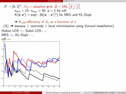
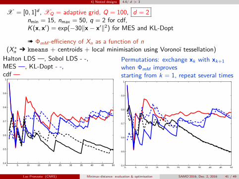
X = [0, 1]d , XQ = adaptive grid, Q = 100, d = 2nmin = 15, nmax = 50, q = 2 for cdf,K (x, x′) = exp(−30‖x− x′‖2) for MES and KL-Dopt
à ΦmM-efficiency of Xn as a function of n(X∗n Ô kmeans + centroids + local minimisation using Voronoï tessellation)
Halton LDS —, Sobol LDS - -,MES —, KL-Dopt - -,cdf —
0 5 10 15 20 25 30 35 40 45 500.4
0.5
0.6
0.7
0.8
0.9
1
Permutations: exchange xk with xk+1when ΦmM improvesstarting from k = 1, repeat several times
0 5 10 15 20 25 30 35 40 45 500.4
0.5
0.6
0.7
0.8
0.9
1
Luc Pronzato (CNRS) Minimax-distance: evaluation & optimisation SAMO’2016, Dec. 2, 2016 41 / 49
4) Nested designs 4.6/ d > 3
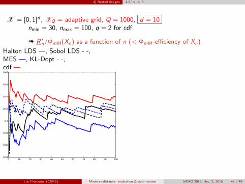
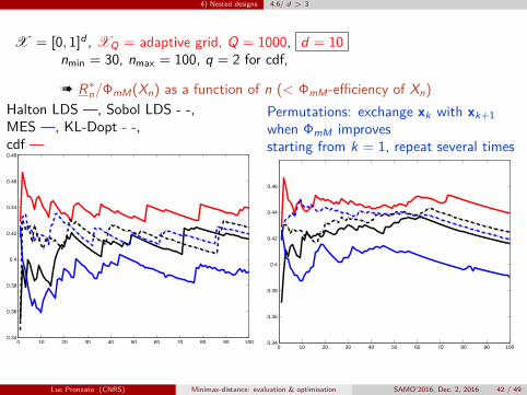
X = [0, 1]d , XQ = adaptive grid, Q = 1000, d = 10nmin = 30, nmax = 100, q = 2 for cdf,
à R∗n/ΦmM(Xn) as a function of n (< ΦmM-efficiency of Xn)Halton LDS —, Sobol LDS - -,MES —, KL-Dopt - -,cdf —
0 10 20 30 40 50 60 70 80 90 1000.34
0.36
0.38
0.4
0.42
0.44
0.46
0.48
Permutations: exchange xk with xk+1when ΦmM improvesstarting from k = 1, repeat several times
0 10 20 30 40 50 60 70 80 90 1000.34
0.36
0.38
0.4
0.42
0.44
0.46
Luc Pronzato (CNRS) Minimax-distance: evaluation & optimisation SAMO’2016, Dec. 2, 2016 42 / 49
4) Nested designs 4.6/ d > 3
X = [0, 1]d , XQ = adaptive grid, Q = 1000, d = 10nmin = 30, nmax = 100, q = 2 for cdf,
à R∗n/ΦmM(Xn) as a function of n (< ΦmM-efficiency of Xn)Halton LDS —, Sobol LDS - -,MES —, KL-Dopt - -,cdf —
0 10 20 30 40 50 60 70 80 90 1000.34
0.36
0.38
0.4
0.42
0.44
0.46
0.48
Permutations: exchange xk with xk+1when ΦmM improvesstarting from k = 1, repeat several times
0 10 20 30 40 50 60 70 80 90 1000.34
0.36
0.38
0.4
0.42
0.44
0.46
Luc Pronzato (CNRS) Minimax-distance: evaluation & optimisation SAMO’2016, Dec. 2, 2016 42 / 49

4) Nested designs 4.7/ To be done. . .
4.7/ To be done. . .Other submodular alternatives to ΦmM :
Take XQ with Q elements, q > 0
a/ φq,a(Xn) =1Q
Q∑k=1
dq(xk ,Xn) (= facility location problem)
b/ φq,b(Xn) =1Q
Q∑k=1
( Q∑i=1‖xk − xi‖−q
)−1
φq,a and φq,b are non-increasing and supermodular, with
Q−1/q ΦmM(Xn) ≤ φ1/qq,a (Xn) ≤ ΦmM(Xn)
(nQ)−1/q ΦmM(Xn) ≤ φ1/qq,b (Xn) ≤ ΦmM(Xn)
[ongoing joint work with João Rendas (CNRS, I3S, UCA) & Céline Helbert (ÉcoleCentrale Lyon), supervision of Ph.D. thesis of Mona Abtini (ECL)Which guarantees on ΦmM-efficiency with a greedy minimisation of φq,a or φq,b?]
Luc Pronzato (CNRS) Minimax-distance: evaluation & optimisation SAMO’2016, Dec. 2, 2016 43 / 49

4) Nested designs 4.7/ To be done. . .
4.7/ To be done. . .Other submodular alternatives to ΦmM :
Take XQ with Q elements, q > 0
a/ φq,a(Xn) =1Q
Q∑k=1
dq(xk ,Xn) (= facility location problem)
b/ φq,b(Xn) =1Q
Q∑k=1
( Q∑i=1‖xk − xi‖−q
)−1φq,a and φq,b are non-increasing and supermodular, with
Q−1/q ΦmM(Xn) ≤ φ1/qq,a (Xn) ≤ ΦmM(Xn)
(nQ)−1/q ΦmM(Xn) ≤ φ1/qq,b (Xn) ≤ ΦmM(Xn)
[ongoing joint work with João Rendas (CNRS, I3S, UCA) & Céline Helbert (ÉcoleCentrale Lyon), supervision of Ph.D. thesis of Mona Abtini (ECL)Which guarantees on ΦmM-efficiency with a greedy minimisation of φq,a or φq,b?]
Luc Pronzato (CNRS) Minimax-distance: evaluation & optimisation SAMO’2016, Dec. 2, 2016 43 / 49

4) Nested designs 4.7/ To be done. . .
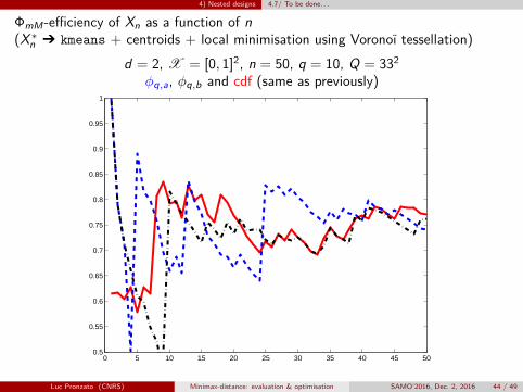
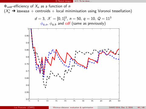
ΦmM-efficiency of Xn as a function of n(X∗n Ô kmeans + centroids + local minimisation using Voronoï tessellation)
d = 3, X = [0, 1]3, n = 50, q = 10, Q = 113φq,a, φq,b and cdf (same as previously)
0 5 10 15 20 25 30 35 40 45 500.5
0.55
0.6
0.65
0.7
0.75
0.8
0.85
0.9
0.95
1
Luc Pronzato (CNRS) Minimax-distance: evaluation & optimisation SAMO’2016, Dec. 2, 2016 44 / 49
4) Nested designs 4.7/ To be done. . .
ΦmM-efficiency of Xn as a function of n(X∗n Ô kmeans + centroids + local minimisation using Voronoï tessellation)
d = 2, X = [0, 1]2, n = 50, q = 10, Q = 332φq,a, φq,b and cdf (same as previously)
0 5 10 15 20 25 30 35 40 45 500.5
0.55
0.6
0.65
0.7
0.75
0.8
0.85
0.9
0.95
1
d = 3, X = [0, 1]3, n = 50, q = 10, Q = 113φq,a, φq,b and cdf (same as previously)
0 5 10 15 20 25 30 35 40 45 500.5
0.55
0.6
0.65
0.7
0.75
0.8
0.85
0.9
0.95
1
Luc Pronzato (CNRS) Minimax-distance: evaluation & optimisation SAMO’2016, Dec. 2, 2016 44 / 49
4) Nested designs 4.7/ To be done. . .
ΦmM-efficiency of Xn as a function of n(X∗n Ô kmeans + centroids + local minimisation using Voronoï tessellation)
d = 3, X = [0, 1]3, n = 50, q = 10, Q = 113φq,a, φq,b and cdf (same as previously)
0 5 10 15 20 25 30 35 40 45 500.5
0.55
0.6
0.65
0.7
0.75
0.8
0.85
0.9
0.95
1
Luc Pronzato (CNRS) Minimax-distance: evaluation & optimisation SAMO’2016, Dec. 2, 2016 44 / 49
4) Nested designs 4.7/ To be done. . .
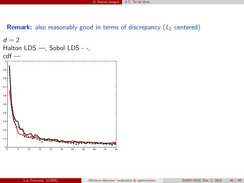
Remark: also reasonably good in terms of discrepancy (L2 centered)
d = 2Halton LDS —, Sobol LDS - -,cdf —
0 5 10 15 20 25 30 35 40 45 500
0.1
0.2
0.3
0.4
0.5
0.6
0.7
0.8
0.9
1
d = 3Halton LDS —, Sobol LDS - -,cdf —
0 5 10 15 20 25 30 35 40 45 500
0.2
0.4
0.6
0.8
1
1.2
1.4
Luc Pronzato (CNRS) Minimax-distance: evaluation & optimisation SAMO’2016, Dec. 2, 2016 45 / 49
4) Nested designs 4.7/ To be done. . .
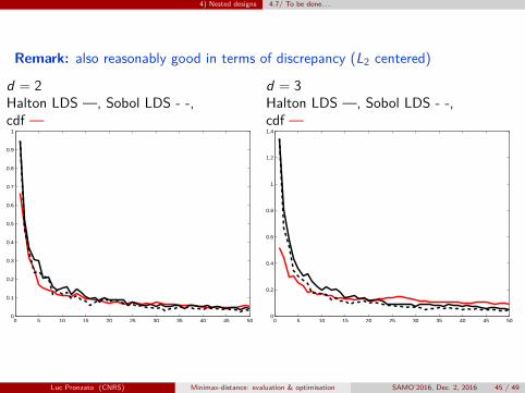
Remark: also reasonably good in terms of discrepancy (L2 centered)
d = 2Halton LDS —, Sobol LDS - -,cdf —
0 5 10 15 20 25 30 35 40 45 500
0.1
0.2
0.3
0.4
0.5
0.6
0.7
0.8
0.9
1
d = 3Halton LDS —, Sobol LDS - -,cdf —
0 5 10 15 20 25 30 35 40 45 500
0.2
0.4
0.6
0.8
1
1.2
1.4
Luc Pronzato (CNRS) Minimax-distance: evaluation & optimisation SAMO’2016, Dec. 2, 2016 45 / 49

5) Conclusions
5) Conclusions
Several methods to evaluate ΦmM(Xn) (MCMC if d ≥ 5)Optimisation by a variant of Lloyd’s method (requires a fixed finite set XQ)
A greedy method (covering measure) to generate nested designs withreasonably good minimax efficiency (better than LDS)
Use an adaptive grid XQ (MCMC) if d is largeKarhunen-Loève decomposition + D-optimal design seems also promising (seeGauthier and Suykens (2016) for constructing sparse low-rank approximations)Can we consider projections on lower dimensional subspaces?Other submodular alternatives?
Fixed n: can we use MCMC with adaptive grid XQ in a Lloyd’s type method?
Luc Pronzato (CNRS) Minimax-distance: evaluation & optimisation SAMO’2016, Dec. 2, 2016 46 / 49

5) Conclusions
5) Conclusions
Several methods to evaluate ΦmM(Xn) (MCMC if d ≥ 5)Optimisation by a variant of Lloyd’s method (requires a fixed finite set XQ)A greedy method (covering measure) to generate nested designs withreasonably good minimax efficiency (better than LDS)
Use an adaptive grid XQ (MCMC) if d is largeKarhunen-Loève decomposition + D-optimal design seems also promising (seeGauthier and Suykens (2016) for constructing sparse low-rank approximations)
Can we consider projections on lower dimensional subspaces?Other submodular alternatives?
Fixed n: can we use MCMC with adaptive grid XQ in a Lloyd’s type method?
Luc Pronzato (CNRS) Minimax-distance: evaluation & optimisation SAMO’2016, Dec. 2, 2016 46 / 49

5) Conclusions
5) Conclusions
Several methods to evaluate ΦmM(Xn) (MCMC if d ≥ 5)Optimisation by a variant of Lloyd’s method (requires a fixed finite set XQ)A greedy method (covering measure) to generate nested designs withreasonably good minimax efficiency (better than LDS)
Use an adaptive grid XQ (MCMC) if d is largeKarhunen-Loève decomposition + D-optimal design seems also promising (seeGauthier and Suykens (2016) for constructing sparse low-rank approximations)Can we consider projections on lower dimensional subspaces?
Other submodular alternatives?
Fixed n: can we use MCMC with adaptive grid XQ in a Lloyd’s type method?
Luc Pronzato (CNRS) Minimax-distance: evaluation & optimisation SAMO’2016, Dec. 2, 2016 46 / 49

5) Conclusions
5) Conclusions
Several methods to evaluate ΦmM(Xn) (MCMC if d ≥ 5)Optimisation by a variant of Lloyd’s method (requires a fixed finite set XQ)A greedy method (covering measure) to generate nested designs withreasonably good minimax efficiency (better than LDS)
Use an adaptive grid XQ (MCMC) if d is largeKarhunen-Loève decomposition + D-optimal design seems also promising (seeGauthier and Suykens (2016) for constructing sparse low-rank approximations)Can we consider projections on lower dimensional subspaces?Other submodular alternatives?
Fixed n: can we use MCMC with adaptive grid XQ in a Lloyd’s type method?
Luc Pronzato (CNRS) Minimax-distance: evaluation & optimisation SAMO’2016, Dec. 2, 2016 46 / 49

5) Conclusions
5) Conclusions
Several methods to evaluate ΦmM(Xn) (MCMC if d ≥ 5)Optimisation by a variant of Lloyd’s method (requires a fixed finite set XQ)A greedy method (covering measure) to generate nested designs withreasonably good minimax efficiency (better than LDS)
Use an adaptive grid XQ (MCMC) if d is largeKarhunen-Loève decomposition + D-optimal design seems also promising (seeGauthier and Suykens (2016) for constructing sparse low-rank approximations)Can we consider projections on lower dimensional subspaces?Other submodular alternatives?
Fixed n: can we use MCMC with adaptive grid XQ in a Lloyd’s type method?
Luc Pronzato (CNRS) Minimax-distance: evaluation & optimisation SAMO’2016, Dec. 2, 2016 46 / 49

References
References I
Auffray, Y., Barbillon, P., Marin, J.-M., 2012. Maximin design on non hypercube domains and kernelinterpolation. Statistics and Computing 22 (3), 703–712.
Cortés, J., Bullo, F., 2005. Coordination and geometric optimization via distributed dynamical systems. SIAMJournal on Control and Optimization 44 (5), 1543–1574.
Cortés, J., Bullo, F., 2009. Nonsmooth coordination and geometric optimization via distributed dynamicalsystems. SIAM Review 51 (1), 163–189.
Du, Q., Faber, V., Gunzburger, M., 1999. Centroidal Voronoi tessellations: applications and algorithms. SIAMReview 41 (4), 637–676.
Fedorov, V., 1996. Design of spatial experiments: model fitting and prediction. In: Gosh, S., Rao, C. (Eds.),Handbook of Statistics, vol. 13. Elsevier, Amsterdam, Ch. 16, pp. 515–553.
Gauthier, B., Pronzato, L., 2014. Spectral approximation of the IMSE criterion for optimal designs inkernel-based interpolation models. SIAM/ASA J. Uncertainty Quantification 2, 805–825, DOI10.1137/130928534.
Gauthier, B., Pronzato, L., 2016. Convex relaxation for IMSE optimal design in random field models.Computational Statistics and Data Analysis (to appear)Hal-01246483.
Gauthier, B., Suykens, J., 2016. A convex relaxation for sparse low-rank Nyström approximation of large scalekernel-matrices. Preprint hal-01323277.
Gonzalez, T., 1985. Clustering to minimize the maximum intercluster distance. Theoretical Computer Science38, 293–306.
Guyader, A., Hengartner, N., Matzner-Løber, E., 2011. Simulation and estimation of extreme quantiles andextreme probabilities. Applied Mathematics & Optimization 64 (2), 171–196.
Luc Pronzato (CNRS) Minimax-distance: evaluation & optimisation SAMO’2016, Dec. 2, 2016 47 / 49

References
References II
Johnson, M., Moore, L., Ylvisaker, D., 1990. Minimax and maximin distance designs. Journal of StatisticalPlanning and Inference 26, 131–148.
Lekivetz, R., Jones, B., 2015. Fast flexible space-filling designs for nonrectangular regions. Quality andReliability Engineering International 31 (5), 829–837.
Lloyd, S., 1982. Least squares quantization in PCM. IEEE Transactions on Information Theory 28 (2),129–137.
Minoux, M., 1977. Accelerated greedy algorithms for maximizing submodular set functions. In: Proc. 8th IFIPConference, Wurzburg (Part 2). Springer, New-York, pp. 234–243.
Mitchell, R., 1990. Error estimates arising from certain pseudorandom sequences in a quasirandom searchmethod. Mathematics of Computation 55 (191), 289–297.
Müller, W., 2007. Collecting Spatial Data. Springer, Berlin, [3rd ed.].Nemhauser, G., Wolsey, L., Fisher, M., 1978. An analysis of approximations for maximizing submodular set
functions–I. Mathematical Programming 14 (1), 265–294.Niederreiter, H., 1992. Random Number Generation and Quasi-Monte Carlo Methods. SIAM, Philadelphia.Pronzato, L., Müller, W., 2012. Design of computer experiments: space filling and beyond. Statistics and
Computing 22, 681–701.Schaback, R., 1995. Error estimates and condition numbers for radial basis function interpolation. Advances in
Computational Mathematics 3 (3), 251–264.Shewry, M., Wynn, H., 1987. Maximum entropy sampling. Applied Statistics 14, 165–170.Spöck, G., Pilz, J., 2010. Spatial sampling design and covariance-robust minimax prediction based on convex
design ideas. Stochastic Environmental Research and Risk Assessment 24 (3), 463–482.
Luc Pronzato (CNRS) Minimax-distance: evaluation & optimisation SAMO’2016, Dec. 2, 2016 48 / 49

References
References III
Sukharev, A., 1992. Minimax Models in the Theory of Numerical Methods. Springer (originally, KluwerAcademic Publishers), Dordrecht.
Vazquez, E., Bect, J., 2011. Sequential search based on kriging: convergence analysis of some algorithms.Proc. 58th World Statistics Congress of the ISI, August 21-26, Dublin, Ireland, arXiv preprintarXiv:1111.3866v1.
Zhigljavsky, A., Hamilton, E., 2010. Stopping rules in k-adaptive global random search algorithms. Journal ofGlobal Optimization 48 (1), 87–97.
Zhigljavsky, A., Žilinskas, A., 2007. Stochastic Global Optimization. Springer, New York.
Luc Pronzato (CNRS) Minimax-distance: evaluation & optimisation SAMO’2016, Dec. 2, 2016 49 / 49


![[6] a Z w ON ^ W0ujSÂ Vó · |snj n t>]Ý n t>]Ý n n 7 n n 7 x=+84.3 x=+84.3 x=+84.5 x=+84.5 x=+84.8 x=+84.8 x=+85.0 x=+85.0 x=+85.3 x=+85.3 x=+85.5 x=+85.5 x=+85.8 x=+85.8 x=+86.0](https://img.pdfslide.us/doc/110x75/6145163534130627ed50c2e6/6-a-z-w-on-w0ujs-v-snj-n-t-n-t-n-n-7-n-n-7-x843-x843.jpg)