GENERALIZED NEWTON-RAPHSON METHOD (GNR) Newton-Raphson Method (GNR) 29 and the new recursion is given by 2 1 ( ( )) ( ) ( ( )) n n n n n n k f x x x f x f x kf x. We call this new

IJMS, Vol. 11, No. 1-2, January-June 2012, pp. 27-41 © Serials Publications

GENERALIZED NEWTON-RAPHSON METHOD (GNR)

Radimir Viher & Nikola Sandri ć

Abstract: We present a new method for solving a non-linear equation f (x) = 0. The methodis derived from the Newton-Raphson tangent method using the ideas of Aitken andSteffensen [5]. It is quadratically convergent and depends on a real parameter k. The classicalNewton-Raphson method appears as the limiting case when k 0. The new method doesnot require the computation of f (x). It is shown that for a convex (concave) function f (x)and suitably chosen small value of k our method converges faster than the classicalNewton-Raphson method with the same initial approximation.

M.S.C. 2000: 65H99, 65B99.

Keywords: Newton-Raphson method, Generalized Newton-Raphson method, Strictlyconvex (concave) function, Aitken’s 2 method, Steffensen’s function.

1. INTRODUCTION

Let (xn)n be a convergent sequence with lim nn

x a . Aitken’s accelerating convergence2 method is based on calculating a new sequence (xn)n defined by formula

2

2

( )nn n

n

xx x

x,

where xn = xn + 1 – xn and 2xn = �( xn). It can be shown that (with the condition xn a,for all n )

lim 0n

n n

x a

x a.

From above we can see that sequence (xn)n is converging faster than (xn)n.

To get faster convergence of a sequence given by a fixed point recursion xn + 1 = (xn),Steffensen introduced function (x) defined by formula

2( ( )) ( ( ))( )

( ( )) 2 ( )x x x

xx x x

.

He showed that functions (x) and (x), with the condition ( ) 1, have the samefixed points and ( ) = 0 in every fixed point of function (x) for which ( ) 1.

28 Radimir Viher & Nikola Sandrić

Definition 1: Let (xn)n be a convergent sequence with lim nn

x . We say that thesequence (xn)n is converging quadratically to � if there exist n0 and C 0 such that

| xn + 1 – | C | xn – |2,

for every n n0.

From ( ) = 0, �( ) = and Taylor’s formula we have

2( )( )

2h

h h .

Let | ( ) |2[ , ]

max x

x l lC . For x0 [ – l, + l] such that C | x0 – | < 1, xn + 1 = (xn)

and hn = xn – we have

| xn + 1 – | C | xn – |2.

According to this, a fixed point iteration for function (x), i.e. xn + 1 = (xn), convergesto quadratically.

With ideas developed from the fixed point iteration we can solve a problem of findingzeros of function f (x). Let be a zero of f (x) and a, b neighborhood of . Suppose thatf (x) does not change the sign on [a, b] and that

0 < m f (x) M, � x [a, b].

Now, if we define function (x) by formula (x) = 1 ( )M

x f x , we have

10 ( ) 1 ( ) 1 1

mx f x

M M.

Due to this, for x0 [a, b] from the Banach fixed point theorem, the iteration

11

( )n n nx x f xM

,

converges to the fixed point , which is also a zero of the function f (x). But this convergenceis not quadratic. To get a quadratic convergence, let’s define a function (x) by formula

(x) = x – kf (x)

and insert (x) in the expression for Steffensens function (x). (The idea to define afunction (x) by x – kf (x) comes from [4]. In [1] one can find the idea to define (x) byx – f (x), but, as we will see, this is not the best possible solution.) We get

2( ( ))( )

( ) ( ( ))k f x

x xf x f x kf x

,

Generalized Newton-Raphson Method (GNR) 29

and the new recursion is given by

2

1( ( ))

( ) ( ( ))n

n nn n n

k f xx x

f x f x kf x.

We call this new recursion the generalized Newton-Raphson method and denote it byGNR. Observe that if we let the constant k to converge to zero we will get

1( )

( )n

n nn

f xx x

f x,

and this is nothing else than the classical Newton-Raphson tangent method. It is necessaryto point out that the condition ( ) = 1 – kf ( ) 1, which is equivalent with f ( ) 0, issaying that the zero is simple. According to this, in every simple zero of function f (x)we have ( ) = 0, and this is independent of the value of constant k.

2. MAIN RESULTS

Theorem 1: Let be a zero of the function f (x). Suppose that f (x) > 0 and f (x) is strictlyconvex and of class C1 on [ , + l] for some l > 0, and suppose that constant k satisfies

[ , ]

10

max ( )x l

kf x

. (1)

Then the sequence

2

1( ( ))

( ) ( ( ))n

n nn n n

k f xx x

f x f x kf x.

with x0 , + l] converges to and the convergence is quadratic.

Proof: First we show that for every x , + l] we have

< x – kf (x). (2)

This is true because for every x , + l] we have

( ) ( )( ) 1

f x fx kf x k

x. (3)

Right hand side in (3) is always satisfied because of condition (1) and Lagrange’smean value theorem.

Inequality (2) implies

2( ( ))( )

( ) ( ( ))n

k f xx x kf x

f x f x kf x, (4)


for every x , + l]. Besides, from (1), Lagrange’s mean value theorem and relation

( ) ( )( ) ( ) 1,

f y f xx kf x y kf y k x y l

y x, (5)

it follows

( ) ( ),x kf x y kf y x y l . (6)

We claim that for every x , + l] we have

2( ( ))( ) ( ( ))

k f xx

f x f x kf x. (7)

Suppose the opposite, i.e.

2( ) ( ( ))( ) ( ) ( ( ))

f x k f xx x

f c f x f x kf x, (8)

wherex – k f (x) < c < x. (9)

Then, because of

( ) ( ) ( )( )

( )

f x f x fx f c

f c x, (10)

and

f (c) k f (x) = f (x) – f (x – k f (x)), (11)

we have

( ) ( ( )) ( ) ( ), , ]

( )nf x f x kf x f x f

x lkf x x

. (12)

But this cannot be true, since from (2) we have that (12) is in contradiction withassumption of the strict convexity of f (x) on [ , + l]. So, (7) is valid.

Let’s form two iterations

2

1( ( ))

( ) ( ( ))n

n nn n n

k f xx x

f x f x kf x

yn + 1 = yn – k f (yn), (13)

for x0 = y0 , + l]. Now, from (4), (5) and (7) we have

2( ( ))( ) ( )

( ) ( ( ))n

n n n n nn n n

k f xx x kf x y kf y

f x f x kf x. (14)


Let’s define function g (x) by formula

g (x) = x – k f (x), x [ , + l]. (15)

From (1) and

g (x) = 1 – kf (x), (16)

we can conclude that g(x) is contraction on [ , + l], i.e.

[ , ]max | ( ) | 1

x lg x . (17)

We conclude that lim nn

y , because is the unique fixed point of g(x) on [ , + l].

Now we see that (14) implies

lim nn

x . (18)

Quadratic convergence of sequence (xn)n follows directly from its construction.

Corollary 1: Suppose that function f (x) on [ , + l] satisfies all conditions of Theorem 1and that the constant k satisfies (1). Then for x0 = y0 , + l] we have

< xn < yn, �n , (19)

where

2

1( ( ))

( ) ( ( ))n

n nn n n

k f xx x

f x f x kf x, (20)

1( )

( )n

n nn

f yy y

f y. (21)

Proof: For n = 1 from (20) and (21) we have

x1 =2

0 00 0

0 0 0 0

( ( )) ( )

( ) ( ( )) ( )

k f x f xx x

f x f x kf x f c,

y1 =0

00

( )

( )

f xx

f x, (22)

where c0 is unique constant in x0 – k f (x0), x0 . Uniqueness of c0 comes from strictlyconvexity of f (x), i.e., f (x) is strictly increasing, on [ , + l].

From f (x0) – f (c0) > 0 ( f (x) is increasing) we have

0 0 0 0 01 1

0 0 0 0

( ) ( ) ( ) ( ( ) ( ))0

( ) ( ) ( ) ( )

f x f x f x f x f cy x

f c f x f c f x. (23)


Using the principle of total induction, and since xn – k f (xn) < cn < xn, we get

yn + 1 – xn + 1 =( ) ( ) ( ) ( )( ) ( ) ( ) ( )

n n n nn n n n

n n n n

f y f x f x f xy x x x

f y f c f x f c

=( ) ( ( ) ( ))

0( ) ( )

n n n

n n

f x f x f c

f c f x. (24)

Second inequality in (24) is a consequence of the fact that the function

( )( )

( )f x

g x xf x

, (25)

is strictly increasing on [ , + l].

From Corollary 1 we can conclude that our method is faster than the classical NRmethod.

Proposition 1: Let the function f (x) be continuous on [a, b] and let f (x) > 0 on a, b .Then for every x [a, b there exists unique function c(x) a, b such that

f (b) – f (x) = f (c(x)) (b – x). (26)

Moreover, for every x a, b we have

( ( ( )) ( ))( )

( ) ( ( ))f c x f x

c xb x f c x

. (27)

Proof: Uniqueness of c (x) follows from Lagrange’s mean value theorem and from thefact that function f (x) is strictly increasing on a, b . The existence of c (x) follows fromthe inverse function derivation theorem because we have

1 ( ) ( )( )

f b f xc x f

b x. (28)

To calculate the derivative of the function c (x), i.e., the formula (27), it suffices only todifferentiate both sides of formulae (26).

Corollary 2: Suppose that the function f (x) satisfies conditions from Theorem 1 onsegment [ , + l] and that f (x) > 0 on , + l , for some l > 0.

Then for any two constants k1 and k2 which satisfy

1 2

[ , ]

10

max ( )x l

k kf x

, (29)


iteration xn(2) with constant k2 is always faster than iteration xn

(1) with constant k1 for sameinitial approximations x0

(1) = x0(2) = x0 , + l].

Proof: First we show that if constant k satisfies condition (1) then the function g(x),defined by

2( ( ))( )

( ) ( ( ))k f x

g x xf x f x kf x

, (30)

is strictly increasing on segment [ , + l]. To prove this first note that the derivative of thefunction h (x) defined by

2( ( ))( )

( ) ( ( ))k f x

h xf x f x kf x

, (31)

is given by

h (x) =2

( ) ( ( )) ( )( ) 2 ( ) ( ( )) (1 ( ))

( )

( ) ( ( ))( )

f x f x kf x f xf x f x f x kf x kf x

f x

f x f x kf xk

kf x

=2 2

( ) (2 ( ) ( ) ( ( )) ( )) ( ) ( ( ))

( ( )) ( ( ))

kf x f c f x f x kf x f x f x f x kf x

k f c k f c

=2 2

( ) (2 ( ) ( ) ( ) ( )) ( ) ( ( ))

( ( )) ( ( ))

f x f c f c kf x f x f x f x kf x

f c k f c

=2

( ) (2 ( ) ( )) ( ) ( ) (1 ( ))

( ( ))

f x f c f x f c f x kf x

f c, (32)

where x – k f (x) < c < x and x – k f (x) < c < x. Note that

g (x) = 1 – h (x), (33)

and hance

g (x) 0 h (x) 1. (34)

From (32) we can see that the condition (34) is equivalent to the condition

f (x) (2f (c) – f (x)) – f (c ) f (x) (1 – k f (x)) ( f (c))2, (35)

i.e., to the condition

0 ( f (x) – f (c))2 + f (c ) f (x) (1 – k f (x)). (36)


It is obvious that (36 ) is true for every x [ , + l]. It is also obvious that inequality(36) becomes equality if and only if x = .

Let us now prove that if we have any two constants k1 and k2, which satisfy (29), thenthe iteration xn

(2) with constant k2 is always faster than the iteration xn(1) with constant k1, for

the same initial approximations x0(1) = x0

(2) = x0 , + l].

First let us take a look what happens in the case n = 1, i.e.

x1(1) =

21 0

00 0 1 0

( ( ))( ) ( ( ))

k f xx

f x f x k f x,

x1(2) =

22 0

00 0 2 0

( ( ))( ) ( ( ))

k f xx

f x f x k f x. (37)

Relations (37) can be written in the form

(1) (2)0 01 0 1 0(1) (2)

0 0

( ) ( ),

( ) ( )

f x f xx x x x

f c f c. (38)

From Proposition 1 and the fact that x0 – k2 f (x0) < x0 – k1 f (x0) we have

C0(2) < C0

(1). (39)

From (38) and (39) we have

(1) (2)(1) (2) 0 0 01 1 (1) (2)

0 0

( ) ( ( ) ( ))0

( ) ( )

f x f c f cx x

f c f c. (40)

Now we prove that (40) is valid for all n using the principle of total induction.Suppose that xn

(1) – xn(2) > 0. Then, as in the case n = 1,

(2) (2) (2) (2)2 1( ) ( )n n n nx k f x x k f x , (41)

implies cn(2) < cn

(1). So, we have

x(1)n + 1 – x(2)

n + 1 >(2) 2 (2) 2

(2) (2)1 2(2) (2) (2) (2) (2) (2)

1 2

( ( )) ( ( ))

( ) ( ( )) ( ) ( ( ))n n

n nn n n n n n

k f x k f xx x

f x f x k f x f x f x k f x

=(2) (2) (2) (1) (2)

(2) (1) (1) (2)

( ) ( ) ( ) ( ( ) ( ))0

( ) ( ) ( ) ( )n n n n n

n n n n

f x f x f x f c f c

f c f c f c f c(42)

The first inequality in (42) is a consequence of strictly increasing property of thefunction g(x).


After all these considerations many questions arise. First of all, suppose that for thefunction f (x) on segment [»; »+l] all the conditions from Corollary 2 are satisfied, andsuppose that k < 0. Now, what can we say about the convergence of sequence (xn)n recursivelydefined by (20)?

We can note that in this situation we need a stronger requirement, i.e., we need that theconditions from Corollary 2 be satisfied on a bigger segment [ , + l + | k | f ( + l)]. Thenfor x0 , + l] we get

20 0 0

0 0 00 0 0 0

( ) ( ) | | ( ( ))( ) ( ) ( | | ( )) ( )

f x f x k f xx x x

f x f c f x k f x f x, (43)

where x0 < c < x0 + | k | f (x0). So, x1 is worse than the first iteration obtained from NRmethod. As in the proof of Corollary 2, before using induction, we have to show thatfunction g(x) defined by the formula

2| | ( ( ))( )

( | | ( )) ( )k f x

g x xf x k f x f x

, (44)

is strictly increasing on segment [ , + l]. To prove this we define function h (x) by

2| | ( ( ))( )

( | | ( )) ( )k f x

h xf x k f x f x

. (45)

By an easy calculation we get

2

( ) (2 ( ) ( )) ( ) ( ) (1 | | ( ( ))( )

( ( ))

f x f c f x f c f x k f xh x

f c. (46)

Obviously, the condition h (x) 1 is equivalent with

0 ( f (x) – f (c))2 + f (c ) f (x) (1 + | k | f (x)). (47)

Note that (47) is satisfied for all x [ , + l], where x < c < x + | k | f (x) andx < c < x + | k | f (x). So, g(x) is increasing on [ , + l]. Note that inequality in (47) becomesequality if and only if x = . From the fact that the function g(x) is strictly increasing on[ , + l] we can easily see that in every iteration step GNR is behind NR. Also, because ofstrictly increasing property of function g(x), the sequence (xn)n is strictly decreasing, i.e.

< xn < xn – 1 < ... < x1 < x0. (48)

Since is the unique fixed point of function x + | k | f (x), i.e. of function g(x) on [ , + l],

we conclude that lim nn

x .


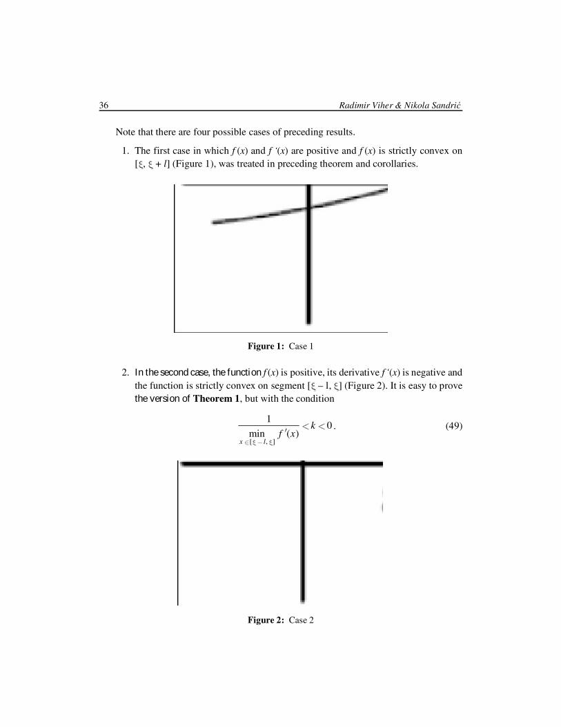
2. In the second case, the function f (x) is positive, its derivative f (x) is negative andthe function is strictly convex on segment [ – l, ] (Figure 2). It is easy to provethe version of Theorem 1, but with the condition

[ , ]

10

min ( )x l

kf x

. (49)

Note that there are four possible cases of preceding results.

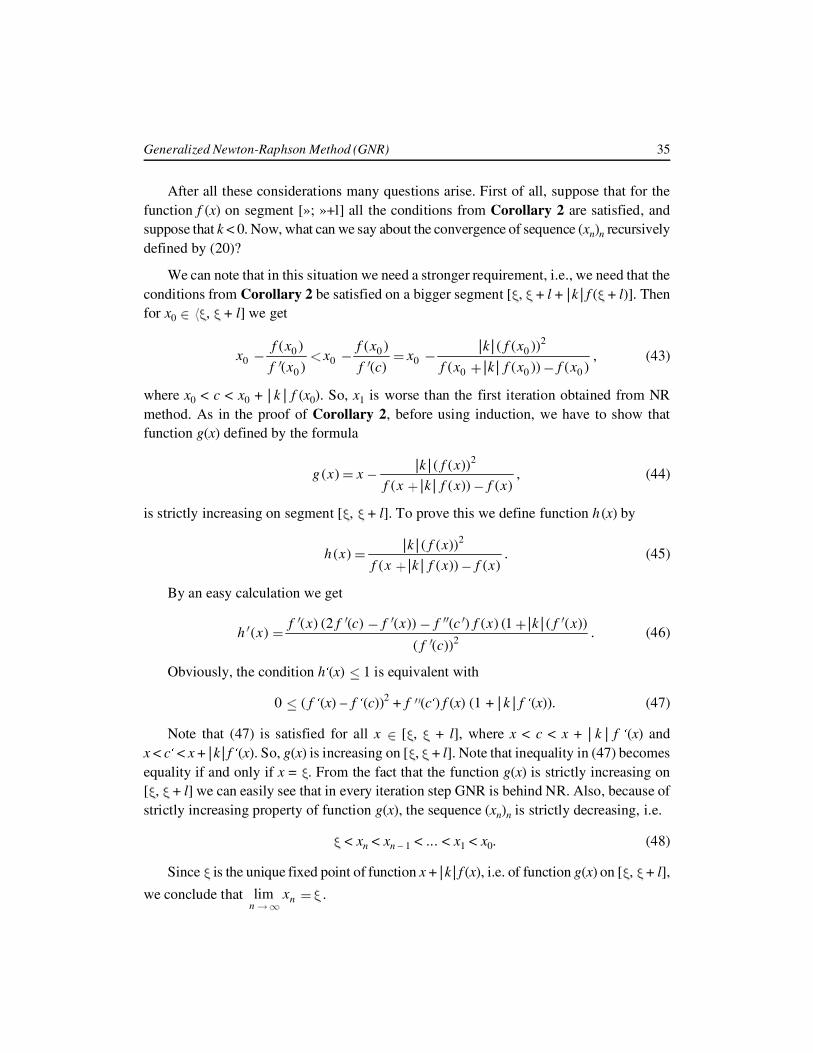
1. The first case in which f (x) and f (x) are positive and f (x) is strictly convex on[ , + l] (Figure 1), was treated in preceding theorem and corollaries.

Figure 1: Case 1

Figure 2: Case 2


In this case, if we take x0 [ – l, , the sequence obtained by GNR convergesquadratically to a zero of the function f (x), and that convergence is faster thanthe NR convergence with the same starting approximation point.

3. In the third case, the function f (x) is negative and strictly concave on segment[ – l, ], while the derivative f (x) is positive on this segment. Similarly as in thesecond case it is easy to prove the version of Theorem 1 but with the condition

[ , ]

10

max ( )x l

kf x

. (50)

For x0 [ – l, the sequence obtained by GNR converges quadratically to a zero of the function f (x), and that convergence is faster than the NR convergence

with the same starting approximation.

4. In the fourth case, the function f (x) is negative and strictly concave on the segment[ , + l] while its derivative f (x) is negative here. In this case we can also provea version of Theorem 1 with the condition

[ , ]

10

min ( )x l

kf x

. (51)

For a given x0 , + l] the sequence obtained by GNR converges quadraticallyto a zero of the function f (x), and this convergence is faster than the NRconvergence with the same starting approximation point.

Note that we can also prove analogous versions of Corollary 1 and Corollary 2or analogous versions of the case when k < 0 for those three cases.

Example 1: Let’s demonstrate our method on the problem of finding square root of 29(this algorithm was known to Heron Alexandrian [1]). We have to find the zeros of thefunction f (x) = x2 – 29 (using the computer with the machine precision = 10–9). The NRfor this problem is given by recursion

11 292n n

n

x xx

.


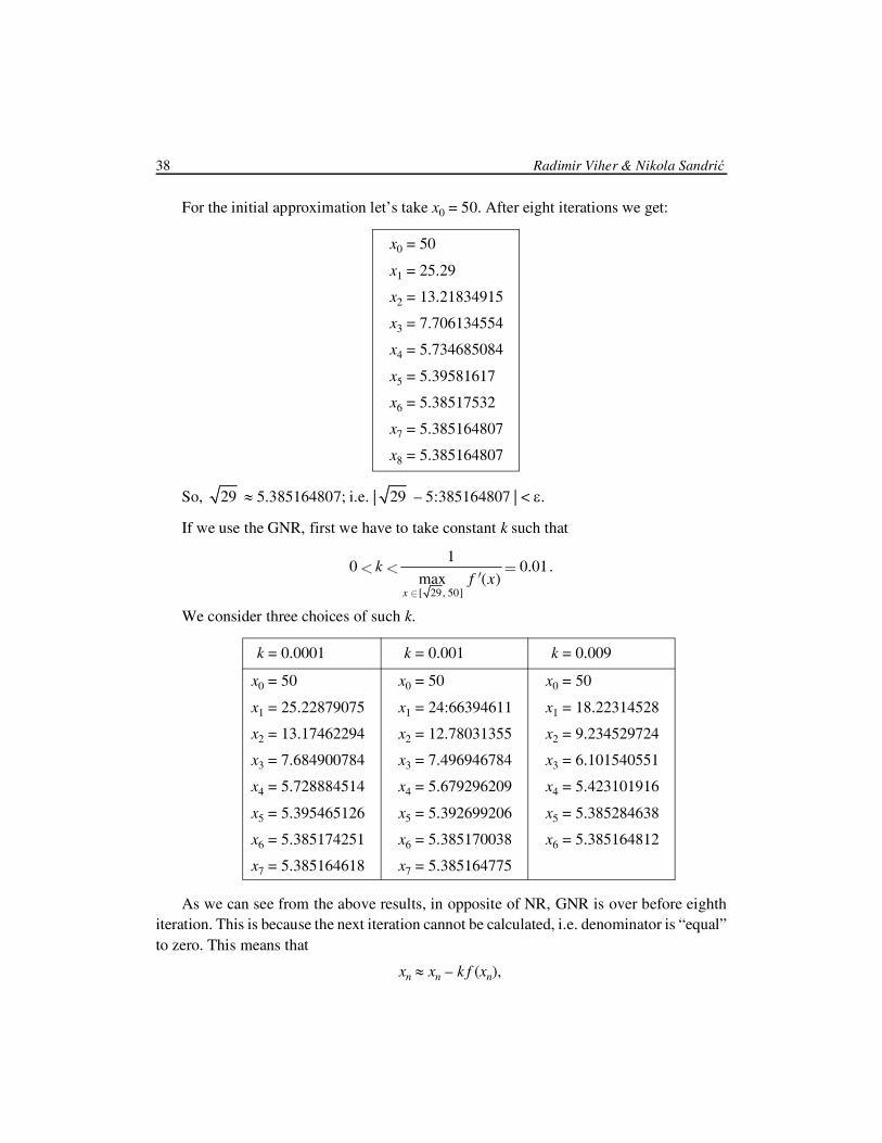
For the initial approximation let’s take x0 = 50. After eight iterations we get:

x0 = 50

x1 = 25.29

x2 = 13.21834915

x3 = 7.706134554

x4 = 5.734685084

x5 = 5.39581617

x6 = 5.38517532

x7 = 5.385164807

x8 = 5.385164807

So, 29 � 5.385164807; i.e. | 29 – 5:385164807 | < �.

If we use the GNR, first we have to take constant k such that

[ 29, 50]

10 0.01

max ( )x

kf x

.

We consider three choices of such k.

k = 0.0001 k = 0.001 k = 0.009

x0 = 50 x0 = 50 x0 = 50

x1 = 25.22879075 x1 = 24:66394611 x1 = 18.22314528

x2 = 13.17462294 x2 = 12.78031355 x2 = 9.234529724

x3 = 7.684900784 x3 = 7.496946784 x3 = 6.101540551

x4 = 5.728884514 x4 = 5.679296209 x4 = 5.423101916

x5 = 5.395465126 x5 = 5.392699206 x5 = 5.385284638

x6 = 5.385174251 x6 = 5.385170038 x6 = 5.385164812

x7 = 5.385164618 x7 = 5.385164775

As we can see from the above results, in opposite of NR, GNR is over before eighthiteration. This is because the next iteration cannot be calculated, i.e. denominator is “equal”to zero. This means that

xn � xn – k f (xn),


i.e., k f (xn) < �. So, the iteration process in GNR can terminate in two possible ways: thedistance of two adjacent iterations is smaller than a given positive constant, or thedenominator in the iteration formula becomes to small.

Also, we can conclude that if constant k increases then calculated zero precision alsoincreases. From Corollary 2. we know that if constant k increases then we get fasterconvergence.

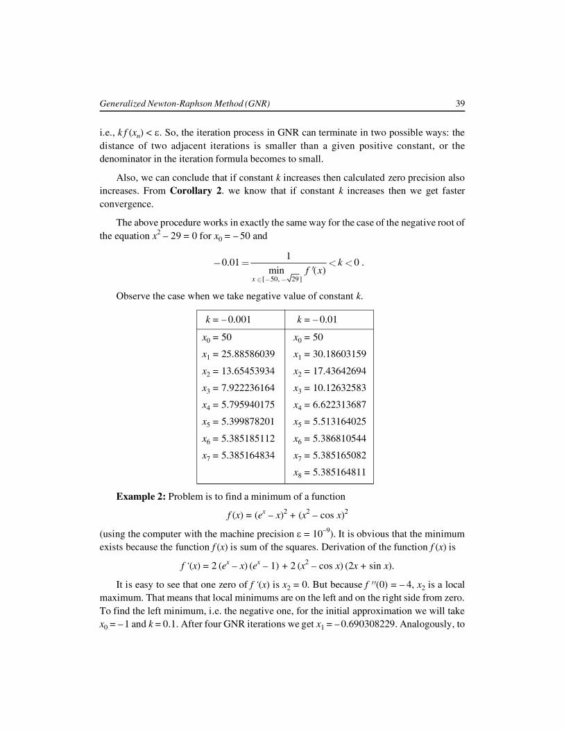
The above procedure works in exactly the same way for the case of the negative root ofthe equation x2 – 29 = 0 for x0 = – 50 and

[ 50, 29]

10.01 0

min ( )x

kf x

.

Observe the case when we take negative value of constant k.

k = – 0.001 k = – 0.01

x0 = 50 x0 = 50

x1 = 25.88586039 x1 = 30.18603159

x2 = 13.65453934 x2 = 17.43642694

x3 = 7.922236164 x3 = 10.12632583

x4 = 5.795940175 x4 = 6.622313687

x5 = 5.399878201 x5 = 5.513164025

x6 = 5.385185112 x6 = 5.386810544

x7 = 5.385164834 x7 = 5.385165082

x8 = 5.385164811

Example 2: Problem is to find a minimum of a function

f (x) = (ex – x)2 + (x2 – cos x)2

(using the computer with the machine precision � = 10–9). It is obvious that the minimumexists because the function f (x) is sum of the squares. Derivation of the function f (x) is

f (x) = 2 (ex – x) (e

x – 1) + 2 (x2 – cos x) (2x + sin x).

It is easy to see that one zero of f (x) is x2 = 0. But because f (0) = – 4, x2 is a localmaximum. That means that local minimums are on the left and on the right side from zero.To find the left minimum, i.e. the negative one, for the initial approximation we will takex0 = – 1 and k = 0.1. After four GNR iterations we get x1 = – 0.690308229. Analogously, to


find the positive minimum, for the initial approximation we will take x0 = 1 and k = 0.1.After four GNR iterations we get x3 = 0.5566918834. Minimum is in x1.

Let’ s take a look at the second derivative of the function f (x), i.e., f (x). From Rolle’stheorem, we know that the function f (x) has to have at least two zeros. The first one mustbe between x1 and x2 and the second one between x2 and x3. To find the negative zero let ustake x0 = – 1 for the initial approximation and k = – 0.1. After five GNR iterations we getx4 = – 0.3983317413. To find the positive zero of f (x), let’s take x0 = 0.4 for the initialapproximation and k = 0.1. After three GNR iterations we get x5 = 0.3190002443.

Example 3: Let us take a look again, at the problem of finding square root of 29, i.e.we have to find the zeros of the function f (x) = x2 – 29 (using the computer with themachine precision = 10–9). But in this example, for the starting approximation point wetake x0 = 2. Note that in this case x0 < 29 . For the constant k such that

[2, 29 ]

10.25

min ( )x

kf x

.

GNR method is behaving like generalized secant method. Generalized secant methodwill be considered in our next paper. If we take k = 0.25 we get the highest speed ofconvergence, i.e. when k is increasing the speed of convergence is decreasing. After fiveiterations we get:

x0 = 2

x1 = 4.439024390

x2 = 5.268806257

x3 = 5.383088524

x4 = 5.385164130

x5 = 5.385164807

With the NR method, for x0 = 2, after six iterations we get x6 = 5.385164807. So we getthe same result as in the NR method, but with faster convergence. One of the reasons forgetting this accuracy is the result of taking x0 from the interval where f (x) f (x) < 0, so theterms in the expression f (xn) – f (xn – kf (xn)) have a different signs. But this will be thesubject of our next paper.

CONCLUSION

In the case of a convex (concave) and class C1 functions, the GNR method converges fasterthan the NR method. Moreover, that convergence is quadratic. Besides, the GNR method


does not require a derivative of the function, as opposed to the NR method. The NR methodcan be considered as a special case of the GNR method, i.e. the NR method appears as thelimiting case when k 0. The constant k has also one nice property, by increasing thevalue of k the accuracy and the convergence speed are increasing, if the value of k is indescribed borders.

ACKNOWLEDGEMENT

The authors thank the professor Tomislav Došlić, Faculty of Civil Engineering, University of Zagreb,for useful comments.

REFERENCES

[1] J. L. Chabert, et al., (1999), A History of Algorithms, Springer, Berlin.

[2] A. Ja. Dorogovcev, (1985), Matematičeski analiz, Viša škola, Kiev.

[3] W. Rudin, (1964), Principles of Mathematical Analysis, Mcgraw-Hill, New York.

[4] M. Schatzmann, (2002), Numerical Analysis, Clarendon Press, Oxford.

[5] J. Stoer, and R. Bulirsch, (1993), Introduction to Numerical Analysis, Springer, New York.

Radimir ViherFaculty of Civil Engineering,University of Zagreb, Zagreb, Croatia,E-mail: [email protected]

Nikola SandrićFaculty of Civil Engineering,University of Zagreb, Zagreb, Croatia,E-mail: [email protected]

Documents

GENERALIZED NEWTON-RAPHSON METHOD (GNR) Newton-Raphson Method (GNR) 29 and the new recursion is given by 2 1 ( ( )) ( ) ( ( )) n n n n n n k f x x x f x f x kf x. We call this new