Embed Size (px)
Citation preview
arX
iv:a
stro
-ph/
0508
531v
1 2
4 A
ug 2
005
On the reliability of merger-trees and the
mass growth histories of dark matter haloes
N. Hiotelis
1st Experimental Lyceum of Athens, Ipitou 15, Plaka, 10557, Athens, Greece,
e-mail: [email protected]
and
A. Del Popolo 1,2
1 Bogazici University, Physics Department, 80815 Bebek, Istanbul, Turkey2 Dipartimento di Matematica, Universita Statale di Bergamo, via dei Caniana, 2,
24127, Bergamo, Italy
e-mail:[email protected]
Abstract
We have used merger trees realizations to study the formation of dark matter haloes.The construction of merger-trees is based on three different pictures about the for-mation of structures in the Universe. These pictures include: the spherical collapse(SC), the ellipsoidal collapse (EC) and the non-radial collapse (NR). The reliabil-ity of merger-trees has been examined comparing their predictions related to thedistribution of the number of progenitors, as well as the distribution of formationtimes, with the predictions of analytical relations. The comparison yields a very sat-isfactory agreement. Subsequently, the mass growth histories (MGH) of haloes havebeen studied and their formation scale factors have been derived. This derivation hasbeen based on two different definitions that are: (a) the scale factor when the haloreaches half its present day mass and (b) the scale factor when the mass growth ratefalls below some specific value. Formation scale factors follow approximately powerlaws of mass. It has also been shown that MGHs are in good agreement with modelsproposed in the literature that are based on the results of N-body simulations. Theagreement is found to be excellent for small haloes but, at the early epochs of theformation of large haloes, MGHs seem to be steeper than those predicted by themodels based on N-body simulations. This rapid growth of mass of heavy haloes islikely to be related to a steeper central density profile indicated by the results ofsome N-body simulations.
Key words: galaxies: halos – formation –structure, methods: numerical –analytical, cosmology: dark matterPACS: 98.62.Gq, 98.62.A, 95.35.+d
Preprint submitted to 31 July 2018
1 Introduction
It is likely that structures in the Universe grow from small initially Gaussiandensity perturbations that progressively detach from the general expansion,reach a maximum radius and then collapse to form bound objects. Largerhaloes are formed hierarchically by mergers between smaller ones.Two different kinds of methods are widely used for the study of the struc-ture formation. The first one is N-body simulations that are able to followthe evolution of a large number of particles under the influence of the mu-tual gravity from initial conditions to the present epoch. The second one issemi-analytical methods. Among these, Press-Schechter (PS) approach and itsextensions (EPS) are of great interest, since they allow us to compute massfunctions (Press & Schechter 1974; Bond et al 1991), to approximate merginghistories (Lacey & Cole 1993, LC93 hereafter, Bower 1991, Sheth & Lemson1999b) and to estimate the spatial clustering of dark matter haloes (Mo &White 1996; Catelan et al 1998, Sheth & Lemson 1999a).In this paper, we present merger-trees based on Monte Carlo realizations. Thisapproach can give significant information regarding the process of the forma-tion of haloes. We focus on the mass growth histories of haloes and we comparethese with the predictions of N-body simulations.This paper is organized as follows: In Sect.2 basic equations are summarized.In Sect.3 the algorithm for the construction of merger-trees as well as testsregarding the reliability of this algorithm are presented. Mass-growth histo-ries are presented in Sect.4, while the results are summarized and discussedin Sect.5.
2 Basic equations and merger-trees realizations
In an expanding universe, a region collapses at time t, if its overdensity atthat time exceeds some threshold. The linear extrapolation of this thresholdup to the present time is called a barrier, B. A likely form of this barrier is asfollows:
B(S, t) =√αS∗[1 + β(S/αS∗)
γ] (1)
1 Present address: Roikou 17-19, Neos Kosmos, Athens, 11743 Greece
2
In Eq.(1) α, β and γ are constants, S∗ ≡ S∗(t) ≡ δ2c (t), where δc(t) is the linearextrapolation up to the present day of the initial overdensity of a sphericallysymmetric region, that collapsed at time t. Additionally, S ≡ σ2(M), whereσ2(M) is the present day mass dispersion on comoving scale containing massM . S depends on the assumed power spectrum. The spherical collapse model(SC) has a barrier that does not depend on the mass (eg. LC93). For this modelthe values of the parameters are α = 1 and β = 0. The ellipsoidal collapsemodel (EC) (Sheth & Tormen 1999, ST99 hereafter) has a barrier that dependson the mass (moving barrier). The values of the parameters are α = 0.707, β =0.485, γ = 0.615 and are adopted either from the dynamics of ellipsoidalcollapse or from fits to the results of N-body simulations. Additionally, the non-radial (NR) model of Del Popolo & Gambera (1998) -that takes into accountthe tidal interaction with neighbors- corresponds to α = 0.707, β = 0.375 andγ = 0.585.Sheth & Tormen (2002) connected the form of the barrier with the form of themultiplicity function. They show that given a mass element -that is a part ofa halo of mass M0 at time t0- the probability that at earlier time t this masselement was a part of a smaller halo with mass M is given by the equation:
f(S, t/S0, t0)dS =1√2π
|T (S, t/S0, t0)|(∆S)3/2
exp
[−(∆B)2
2∆S
]dS (2)
where ∆S = S−S0 and ∆B = B(S, t)−B(S0, t0) with S = S(M), S0 = S(M0).The function T is given by:
T (S, t/S0, t0) = B(S, t)−B(S0, t0) +5∑
n=1
[S0 − S]n
n!
∂n
∂SnB(S, t). (3)
Setting S0 = 0, and B(S0, t0) = 0 in Eq. 3, we can predict the unconditionalmass probability f(S, t), that is the probability that a mass element is a part ofa halo of mass M , at time t. The quantity Sf(S, t) is a function of the variableν alone, where ν ≡ δc(t)/σ(M). Since δc and σ evolve with time in the sameway, the quantity Sf(S, t) is independent of time. Setting 2Sf(S, t) = νf(ν),one obtains the so-called multiplicity function f(ν). The multiplicity functionis the distribution of first crossings of a barrier B(ν) by independent uncor-related Brownian random walks (Bond et al. 1991). That is why the shape ofthe barrier influences the form of the multiplicity function. The multiplicityfunction is related to the comoving number density of haloes of mass M attime t -N(M, t)- by the relation,
νf(ν) =M2
ρb(t)N(M, t)
d lnM
d ln ν(4)
3
that results from the excursion set approach (Bond et al. 1991). In Eq.4, ρb(t)is the density of the model of the Universe at time t.Using a barrier of the form of Eq.1 in the unconditional mass probability, thefollowing expression for f(ν) is found:
f(ν) =√2α/π[1 + β(αν2)−γg(γ)] exp
(−0.5aν2[1 + β(αν2)−γ ]2
)(5)
where
g(γ) =| 1− γ +γ(γ − 1)
2!− ...− γ(γ − 1) · · · (γ − 4)
5!| (6)
0.5 1 1.5 2 2.5 3 3.5 4ν
0.1
0.2
0.3
0.4
0.5
f()
v
νν
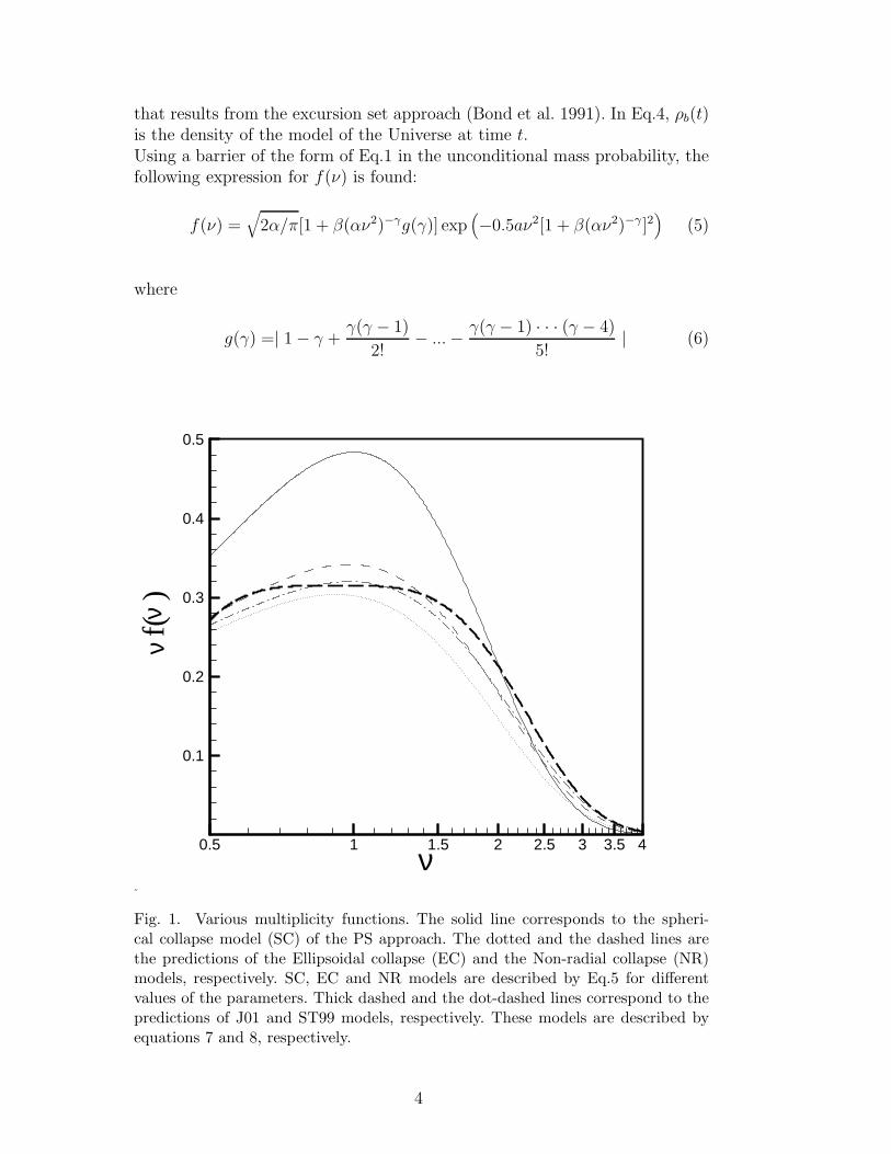
Fig. 1. Various multiplicity functions. The solid line corresponds to the spheri-cal collapse model (SC) of the PS approach. The dotted and the dashed lines arethe predictions of the Ellipsoidal collapse (EC) and the Non-radial collapse (NR)models, respectively. SC, EC and NR models are described by Eq.5 for differentvalues of the parameters. Thick dashed and the dot-dashed lines correspond to thepredictions of J01 and ST99 models, respectively. These models are described byequations 7 and 8, respectively.
4
In Fig.1 we plot νf(ν) versus ν. The solid line results from Eq. 5 for the valuesof the parameters that correspond to the SC model. The dotted line is derivedfrom the values of EC model while the dashed line corresponds to the NRmodel. For matter of completeness, we draw two more lines. The first line, theone with thick dashes- corresponds to the function of Jenkins et al. (2001, J01hereafter). This satisfies the following equation:
νf(ν) = 0.315exp(− | 0.61 + ln[σ−1(M)] |3.8) (7)
In order to express the above relation as a function of ν, we substitute σ−1(M) =ν/δc and we assume a constant value of δc, that of the Einstein-de Sitter Uni-verse, namely δc = 1.686. The above formula is valid for 0.5 ≤ ν ≤ 4.8. Thesecond additional line, dot-dashed one, is the function proposed by ST99 andis:
νf(ν) = A(1 + ν ′−2p)√2/πν ′exp(−ν ′2/2) (8)
where ν ′ = ν√α and the values of the constants are: A = 0.322, p = 0.3 and
α = 0.707.We have noted that the comparison of the above curves with the results ofN-body simulations is in a very good agreement, except for the SC model.Such a comparison is presented by Yahagi et al. (2004). According to theirresults, the numerical multiplicity functions reside between the ST99 and J01multiplicity functions at ν ≥ 3 and are below the ST99 function at ν ≤ 1. Ad-ditionally, the numerical multiplicity functions have an apparent peak at ν ∼ 1-as those given by Eq. 5- instead of the plateau that is seen in the J01 function.
3 The construction of merger-trees
Let there be a number of haloes with the same present day mass M0. Thepurpose of merger-trees realizations is to study the past of these haloes. Thisis done by finding the distribution of their progenitors (haloes that mergedand formed the present day haloes) at previous times. A way to do this is byusing Eq.2. First of all, one has to use a model for the Universe and a powerspectrum. In what follows we have assumed a flat model for the Universe withpresent day density parameters Ωm,0 = 0.3 and ΩΛ,0 ≡ Λ/3H2
0 = 0.7 whereΛ is the cosmological constant and H0 is the present day value of Hubble’sconstant. We used the value H0 = 100 hKMs−1Mpc−1 with h = 0.7 and a sys-tem of units with munit = 1012M⊙h
−1, runit = 1h−1Mpc and a gravitationalconstant G = 1. At this system of units H0/Hunit = 1.5276.Regarding the power spectrum- that defines the relation between S and M
5
in Eq.2- we employed the ΛCDM formula proposed by Smith et al. (1998).The power spectrum is smoothed using the top-hat window function and isnormalized for σ8 ≡ σ(R = 8h−1Mpc) = 1.For each one of the SC, EC and NR models, we studied four different cases.These four cases differ to the present day mass of the haloes under study andare denoted as SC1, SC2, SC3, SC4 for the SC model, EC1, EC2, EC3 andEC4 for the EC model and NR1, NR2, NR3 and NR4 for the NR model. Thefirst case of each model (SC1, EC1 and NR1) corresponds to haloes with mass0.1 -measured in our system of units- while the second case (SC2, EC2 andNR2) corresponds to mass 1. SC3, EC3, NR3 correspond to haloes with mass10 and SC4, EC4, NR4 correspond to masses 100.Pioneered works for the construction of merger-trees are those of LC93, Somerville& Kollat (1999), ST99 and van de Bosch (2002, vdB02). Many of their ideasare used for the construction of our algorithm, that is described below.First, let us define as Nres, the number of realizations used. This number isthe total number of present day haloes of given mass M0. A mass cutoff Mmin
is used, that is a lower limit for the mass of progenitors. No progenitors withmass less than Mmin exist in the merger history of a halo. Mmin is set to afixed fraction of M0. In what follows, Mmin = 0.05M0 (see also vdB02). Also,amin is the minimum value of the scale factor. We set amin = 0.1. Merginghistories do not extend to values of a < amin. A discussion about the choiceof amin is given in Section 4.Useful matrices which have been used are the following: Mpar (the masses ofthe parent haloes), Ml (the masses that are left to be resolved) and Mpro (themasses of the progenitors). The argument i takes the values from 1 to Nmax,where Nmax is the number of haloes that are going to be resolved. Initially,Nmax = Nres. The values of ∆ω, Nres, Mmin, amin are used as input. Wediscuss the choice of the value of ∆ω in Section 4. The scale factor a is set toits initial value, (that is the present day one), a = a0 = 1. Then, the matricesMpar and Ml take their values: Mpar(i) = M0, Ml(i) = M0 for i = 1, Nres. Itis convenient to set a counter for the number of time steps, so we set Istep = 0.The rest of the procedure consists of the following steps:1st step: Istep = Istep + 1.The equation δc(ap) = ∆ω + δc(a) is solved for ap, that is the new, (current)value of the scale factor.2nd step: for i = 1, Nmax
3rd step A value of ∆S is chosen from the desired distribution.4th step: The mass Mp of the progenitor is found, solving for Mp the equa-tion: ∆S = S(Mp) − S(Mpar(i)). If Mp ≥ Ml(i) then, we return to the 3rdstep. Else, the halo with mass Mp is a progenitor of the parent halo i . Themass to be resolved is now given by: Ml(i) = Ml(i)−Mp. If Mp < Mmin thenMp is too small and is not considered as a real progenitor, therefore we returnto the 3rd step. Else,5th step: The number of progenitors is increased by one, (Npro = Npro + 1),and the new progenitor is stored to the list Mpro(Npro) = Mp.
6
6th step: If the mass left to be resolved exceeds the minimum mass, (Ml(i) >Mmin), we go back to the 3rd step. Else, we return to the 2nd step, where thenext value of i is treated.7th step: We set the new number of haloes Nmax to be the number of pro-genitors, Nmax = Npro. We store the progenitors, Mpro(j), j = 1, Nmax. Themasses of new parents are defined as the masses of progenitors by Mpar(j) =Mpro(j), j = 1, Nmax. The value of the scale factor is updated a = ap, as wellas the mass left to be resolved, Ml(j) = Mpar(j), i = j, Nmax. If a ≤ amin westop. Else, we return to the first step.Output is the list of progenitors after a desired number of time steps. Re-garding the third step, we have the following remarks. For the SC case, thechange of variables x ≡ δc(t)−δc(t0)√
S(M)−S(M0)leads to a Gaussian distribution with
zero mean value and unit variance for the new variable x. So, we pick valuesx from the above Gaussian (that is the well-known and very fast procedurePress et al. 1990). The values of ∆S = x∆ω are distributed according to thedistribution described in Eq. 2. The distributions in the EC and NR casescannot be expressed using a Gaussian, so a more general method is used. Thismethod, described in Press et al. (1990) is as follows:Let’s suppose that we would like to pick numbers from a distribution functionG(x), where the variable x takes positive values in the interval [0, c]. First,we calculate the integral
∫ c0 G(t)dt = A. We note that A is not necessarily
equal to unity. Then, a number, let say y, between zero and A is picked froma uniform distribution. The integral equation:
x∫
0
G(t)dt = y (9)
is solved for x. The resulting points (x,G(x)) are then uniformly distributed inthe area between the graph of G, the x-axis and the lines x = 0 and x = c. Thevalues of x have the desired distribution. We have to note that this procedureis -as it is expected- more time demanding than the SC. This is mainly due tothe numerical solution of the integral equation. However, it has the advantageof being general.In Eq.2, f becomes an one variable function for given values of S0, t0, andt. Then, the above described general procedure is used in order to pick val-ues of S. For numerical reasons, it is convenient to use a new variable w =1/√S − S0.
The distribution of the masses of progenitors is found using the following pro-cedure: Let Np be the number of progenitors of Nres parent haloes at time tand let mmin, mmax be the minimum and the maximum mass of these pro-genitors, respectively. We divide the interval [mmin, mmax] to a set of kmax
intervals of length ∆m. Then, the number of progenitors, Npro,k, in the in-terval [mmin + k∆m, mmin + (k + 1)∆m] for k = 0, kmax − 1 is found. The
7
distribution of progenitors masses is then given by Nm−tree ≡ Npro,k
∆mNres. This
distribution has to be compared with the distribution that results from theanalytical relations. Thus, multiplying Eq.2 by M0/M , one finds the expectednumber of progenitors at t that lie in the range of masses M, M + dM . Thisnumber obeys the equation:
N(M, t/M0, t0)dM =M0
Mf(S, t/S0, t0) |
dS
dM| dM (10)
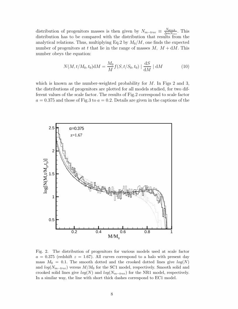
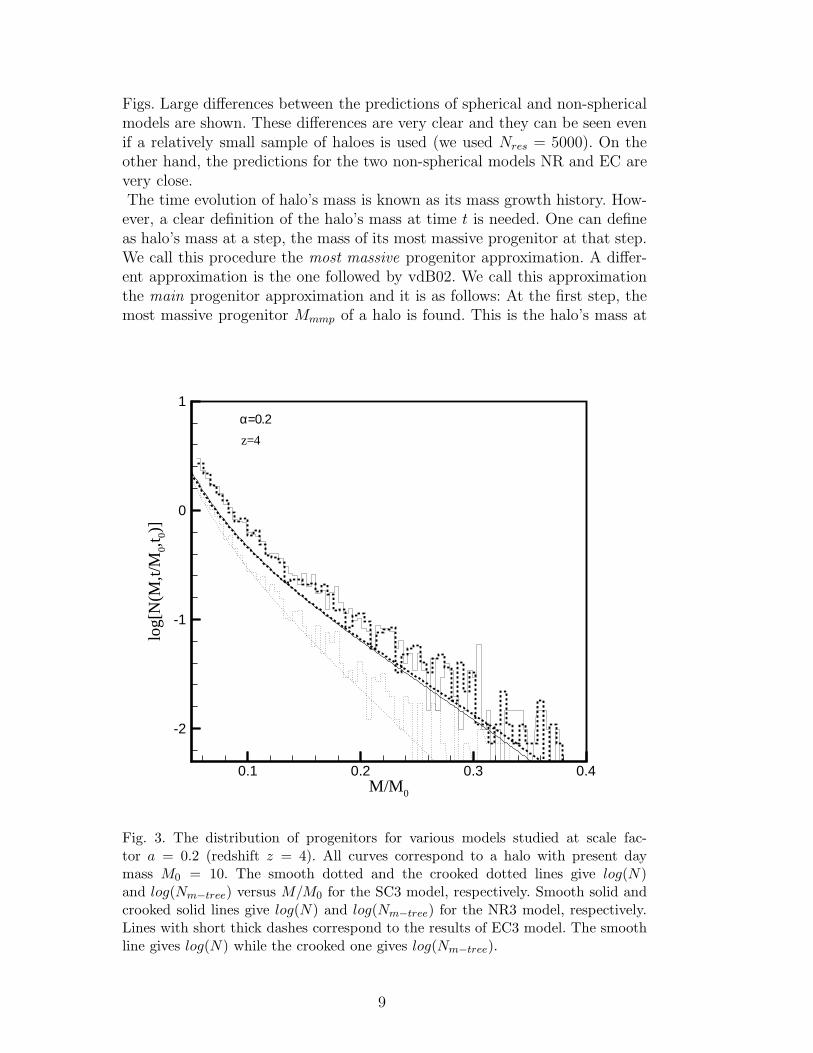
which is known as the number-weighted probability for M . In Figs 2 and 3,the distributions of progenitors are plotted for all models studied, for two dif-ferent values of the scale factor. The results of Fig.2 correspond to scale factora = 0.375 and those of Fig.3 to a = 0.2. Details are given in the captions of the
0.2 0.4 0.6 0.8 1M/M0
0.5
1
1.5
2
2.5
log[
N(M
,t/M
0,t 0)
]
α=0.375z=1.67
Fig. 2. The distribution of progenitors for various models used at scale factora = 0.375 (redshift z = 1.67). All curves correspond to a halo with present daymass M0 = 0.1. The smooth dotted and the crooked dotted lines give log(N)and log(Nm−tree) versus M/M0 for the SC1 model, respectively. Smooth solid andcrooked solid lines give log(N) and log(Nm−tree) for the NR1 model, respectively.In a similar way, the line with short thick dashes correspond to EC1 model.
8
Figs. Large differences between the predictions of spherical and non-sphericalmodels are shown. These differences are very clear and they can be seen evenif a relatively small sample of haloes is used (we used Nres = 5000). On theother hand, the predictions for the two non-spherical models NR and EC arevery close.The time evolution of halo’s mass is known as its mass growth history. How-ever, a clear definition of the halo’s mass at time t is needed. One can defineas halo’s mass at a step, the mass of its most massive progenitor at that step.We call this procedure the most massive progenitor approximation. A differ-ent approximation is the one followed by vdB02. We call this approximationthe main progenitor approximation and it is as follows: At the first step, themost massive progenitor Mmmp of a halo is found. This is the halo’s mass at
0.1 0.2 0.3 0.4M/M0
-2
-1
0
1
log[
N(M
,t/M
0,t 0)
]
α=0.2z=4
Fig. 3. The distribution of progenitors for various models studied at scale fac-tor a = 0.2 (redshift z = 4). All curves correspond to a halo with present daymass M0 = 10. The smooth dotted and the crooked dotted lines give log(N)and log(Nm−tree) versus M/M0 for the SC3 model, respectively. Smooth solid andcrooked solid lines give log(N) and log(Nm−tree) for the NR3 model, respectively.Lines with short thick dashes correspond to the results of EC3 model. The smoothline gives log(N) while the crooked one gives log(Nm−tree).
9
that time. At the next step, the most massive progenitor of the halo withmass Mmmp is found and is considered as the new halo’s mass. The procedureis repeated for the next steps. According to the definition of LC93, the scalefactor at which the mass of the main progenitor equals half the present daymass of the halo is called the formation scale factor. We denote it by af . Adetailed description of the procedure follows:1st step: Istep = Istep + 1.The equation δc(ap) = ∆ω + δc(a) is solved for ap that is the new (current)value of the scale factor.2nd step:for i = 1, Nmax
The mass of the most massive progenitor of parent i is set equal to zero(Mmmp(i) = 0).3rd. A value of ∆S from the desired distribution is chosen.4th step: A mass Mp is found, solving for Mp the equation: ∆S = S(Mp)−S(Mpar(i)). If Mp ≥ Ml(i) then, we go back to the 3rd step. Else, the halowith mass Mp is a progenitor. We set Ml(i) = Ml(i)−Mp. If Mp < Mmin thenMp is too small and is not considered as a real progenitor and so we return tothe 3rd step. Else,5th step: The most massive progenitor at this time step is found.Mmmp(i) = max(Mp,Mmmp(i)).6th step: If the mass left to be resolved exceeds the minimum mass, (Ml(i) >Mmin), we go back to the third step. Else, we check if the mass of the mostmassive progenitor is for the first time smaller than half the initial mass of thehalo. If this is correct, then the formation scale factor of this halo is definedby linear interpolation:
aform(i) = ap +0.5M0 −Mmmp(i)
Mpar(i)−Mmmp(i)(a− ap) (11)
Otherwise, we proceed with the next i.7th step: The list of the most massive progenitors is used, in order to find themean mass at this time step. The time of the scale factor is updated a = ap, aswell as the mass left to be resolved, Ml(j) = Mpar(j), j = 1, Nres. If a ≤ amin
we stop, else we go to the first step.We have to note that the halo’s mass at a step -derived by the above procedure-does not give the mass of its most massive progenitor at that step. For example,let a halo of mass M0 that has at the first step two progenitors with massesM1 and M2 with M1 > M2. Then, the mass of the halo at the second step isdefined as the mass of the most massive progenitor (M1). This progenitor isnot necessarily the most massive of all progenitors at that step, since it couldbe less massive than one of the progenitors of M2. The procedure of main
progenitor described above has the advantage of being economic. It does notrequire the construction of a complete set of progenitors in order to find themost massive one at a step.
10
We tested both the most massive and the main progenitor approximationsand we found small differences only for massive haloes. In order to be able tocompare our results with those of other authors, we used the main progenitorapproximation.A test for the reliability of merger-trees is the comparison of the distributionof formation scale factors with the one given by the analytical relations thatfollow. The probability that the mass of the progenitor, at time t, is largerthan M0/2 is given by:
P (t,Mp > M0/2) =
M0∫
M0/2
N(M, t/M0, t0)dM (12)
The formation time is defined (LC93) as the epoch when the mass of thehalo, as it grows by mergers with other haloes, crosses the half of its presentday value. Then, P (t,Mp > M0/2) is the probability the halo with presentday mass M0 had a progenitor heavier than M0/2 at t, which is equivalentto the probability that the halo is formed earlier than t, P (< t,M0). Thus,P (t,Mp > M0/2) = P (< t,M0). Differentiating with respect to t, we obtain:
dP (< t,M0)
dt=
M0∫
M0/2
∂
∂t[N(M, t/M0, t0)] dM (13)
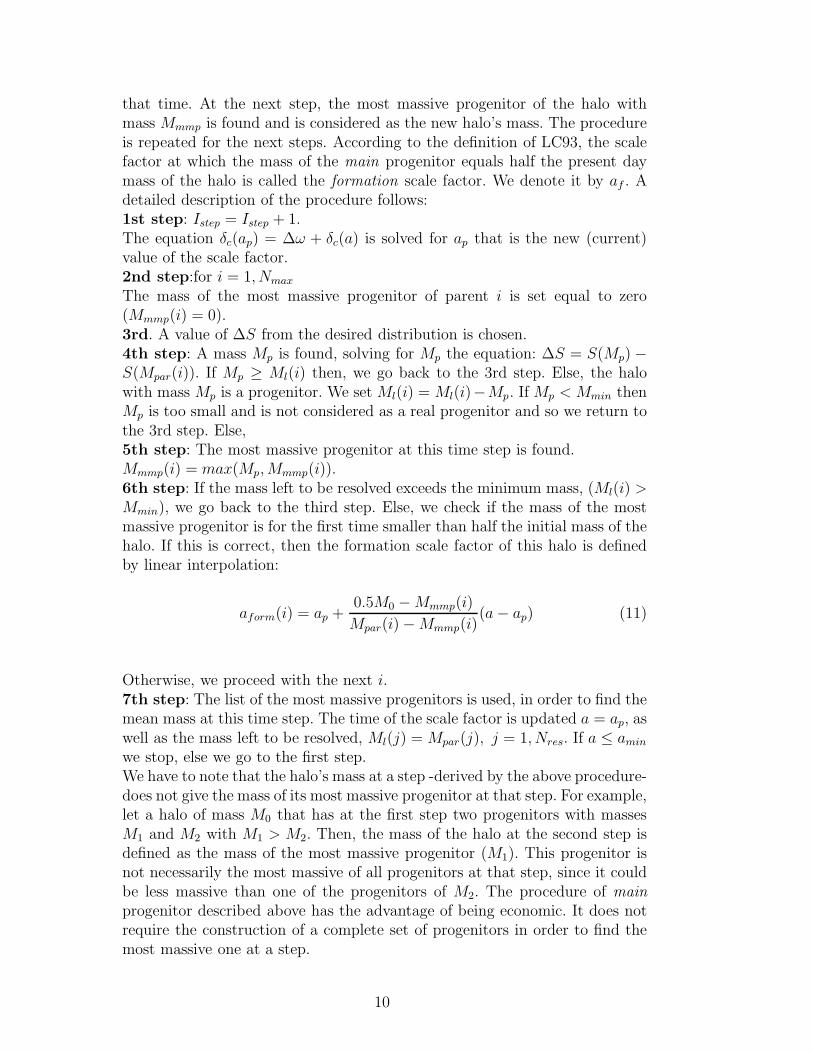
which gives the distribution of formation times.The distribution of formation scale factors as it results from Eq.13 is plottedin Fig. 4. The left hand side snapshot corresponds to haloes with present day
0.2 0.4 0.6 0.8α
0
0.5
1
1.5
2
2.5
3
3.5
4
dP
/dα
0.2 0.4 0.6 0.8α
0
0.5
1
1.5
2
2.5
3
dP/d
α
α
Fig. 4. The distribution of formation scale factors as it results from Eq.13 for thethree models used in this paper. The dotted lines correspond to the SC model, thesolid ones to the NR model and the dashed to the EC model. The left snapshotcorresponds to haloes with present day mass 0.1 -in our system of units- while theright snapshot to haloes with present day mass 100.
11
0.2 0.4 0.6 0.8 1
α0
0.5
1
1.5
2
2.5
3
3.5
dP/d
SC1-NR1
α
0.4 0.6 0.8 1
α0
0.5
1
1.5
2
2.5
3
dP/d
SC4-NR4
α
0.2 0.4 0.6 0.8 1
α0
0.5
1
1.5
2
2.5
3
3.5dP
/dSC1-EC1
α
0.4 0.6 0.8 1
α0
0.5
1
1.5
2
2.5
3
dP/d
SC4-EC4
α
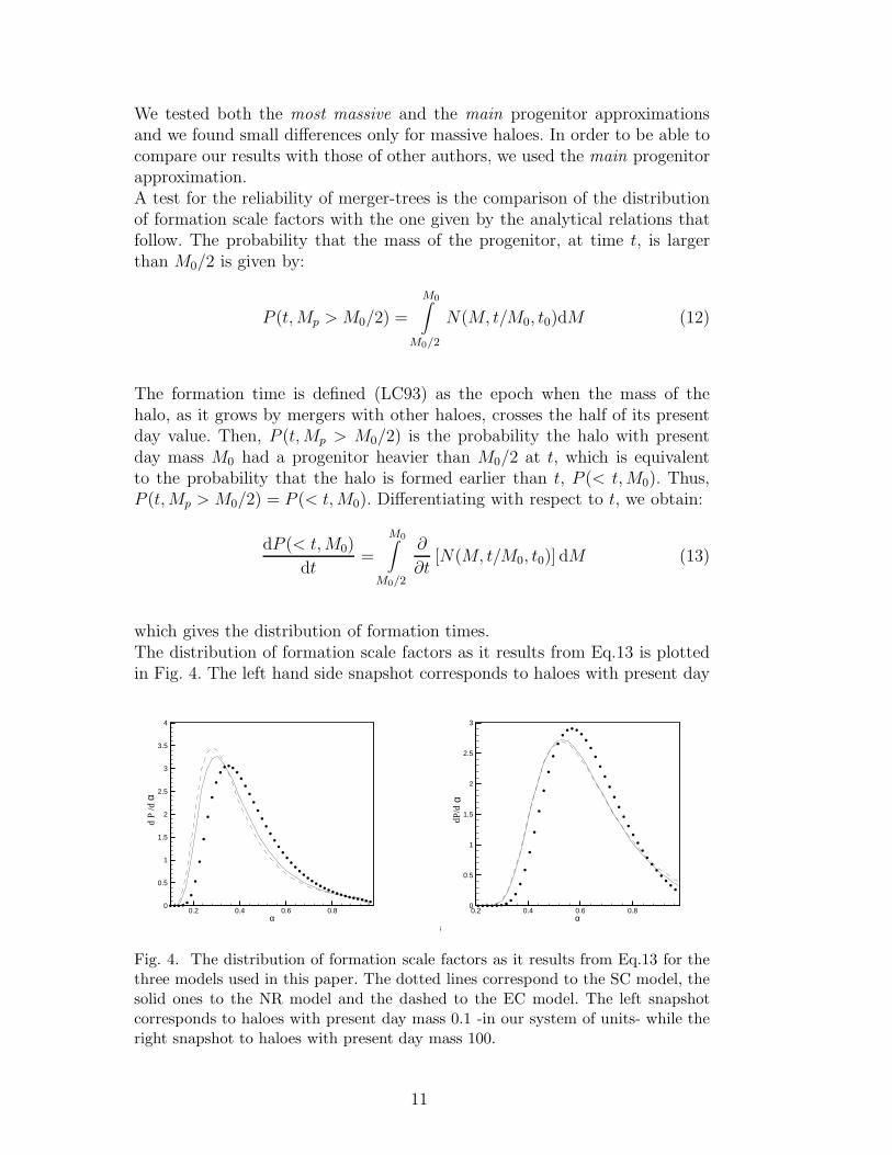
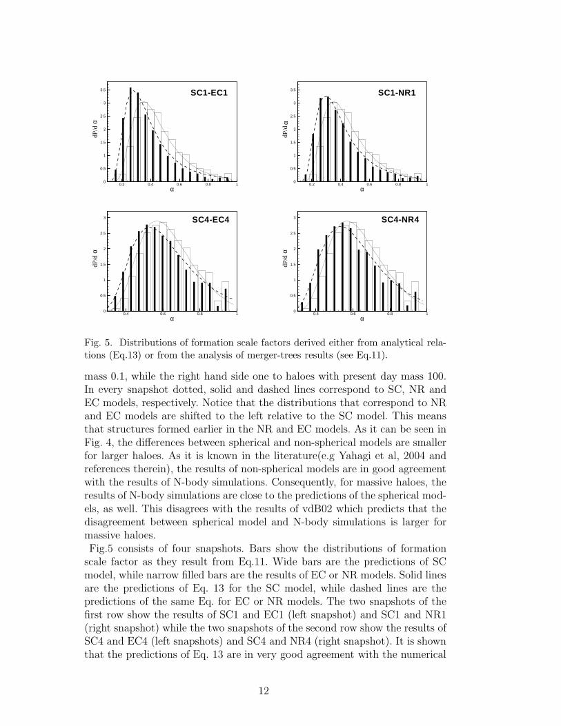
Fig. 5. Distributions of formation scale factors derived either from analytical rela-tions (Eq.13) or from the analysis of merger-trees results (see Eq.11).
mass 0.1, while the right hand side one to haloes with present day mass 100.In every snapshot dotted, solid and dashed lines correspond to SC, NR andEC models, respectively. Notice that the distributions that correspond to NRand EC models are shifted to the left relative to the SC model. This meansthat structures formed earlier in the NR and EC models. As it can be seen inFig. 4, the differences between spherical and non-spherical models are smallerfor larger haloes. As it is known in the literature(e.g Yahagi et al, 2004 andreferences therein), the results of non-spherical models are in good agreementwith the results of N-body simulations. Consequently, for massive haloes, theresults of N-body simulations are close to the predictions of the spherical mod-els, as well. This disagrees with the results of vdB02 which predicts that thedisagreement between spherical model and N-body simulations is larger formassive haloes.Fig.5 consists of four snapshots. Bars show the distributions of formationscale factor as they result from Eq.11. Wide bars are the predictions of SCmodel, while narrow filled bars are the results of EC or NR models. Solid linesare the predictions of Eq. 13 for the SC model, while dashed lines are thepredictions of the same Eq. for EC or NR models. The two snapshots of thefirst row show the results of SC1 and EC1 (left snapshot) and SC1 and NR1(right snapshot) while the two snapshots of the second row show the results ofSC4 and EC4 (left snapshots) and SC4 and NR4 (right snapshot). It is shownthat the predictions of Eq. 13 are in very good agreement with the numerical
12
distributions. Additionally, it is clear that the differences between the distri-butions of various models, resulting from Eq. 13, are successfully reproducedby numerical distributions. It is also shown that differences between sphericaland non-spherical models are more significant for haloes of small mass.
4 Mass-growth histories
We define as mass-growth history, MGH, of a halo with present-day mass M0,the curve that shows the evolution of M(a) ≡< M(a) > /M0 where < M(a) >is the mean mass at scale factor a of haloes with present day mass M0. Twoinput parameters are used in the method of construction merger-trees in theprocedure described in the previous section. The first one is the ’time-step’∆ω. For values of ∆ω ≤ 0.3, it is shown (vdB02) that MGHs are not time-stepdependent. According to that, we used a value ∆ω = 0.1. The second param-eter is amin. Our results are derived for amin = 0.1. In order to justify thischoice, let us discuss the following points regarding the definition of the meanmass. Let Nh(a) be the number of haloes at scale factor a that have massesgreater than Mmin. Obviously, Nh(1) = Nres. Let also Mh,i(a) be the mass ofthe ith halo at scale factor a. We define by Mk(a) the sum
∑Mh,i(a), where
for k = 1 the sum is extended to all haloes that satisfy Mh,i(a) ≥ Mmin. Fork = 2 the sum is extended to all haloes (obviously in that case, the masses of anumber of haloes are equal to zero since, by the construction of merger-trees,their mass histories are not followed beyond Mmin). Finally, for k = 3 the sumis over those haloes that satisfy Mh,i(amin) ≥ Mmin. Then, we can define themean mass at a in three different ways: First Mmean
1 = M1(a)/Nh(a), secondMmean
2 = M2(a)/Nres and third Mmean3 = M3(a)/Nh(amin).
As a evolves from its present day value to smaller values, the number Nh(a)becomes smaller and the three mean values defined above become different.It is clear that Mmean
1 overestimates the mean value, while Mmean2 underesti-
mates it. On the other hand, Mmean3 requires a large number of Nres so that
the remaining sample of haloes Nh(amin) to be large enough. The choice ofthe value amin = 0.1 is justified by the fact that for a ≥ amin the differencesin the above three definitions are negligible.The following results have been derived using a number of 10000 haloes. Wefound that a number of haloes greater than 1000 is sufficient for producingsmooth MGHs that are in exact agreement with the ones of our results.Fig.6 consists of three snapshots. The first snapshot shows the results of theSC model. The other two snapshots correspond to the EC and to the NRmodel, respectively. Every snapshot contains four lines. From top to bottomthese lines correspond to the cases 1, 2, 3 and 4, respectively. It is clear that -atpresent time- the slopes that correspond to smaller masses are smaller. Thissequence of slopes is a sequence of formation times. Large haloes continue
13
-1 -0.8 -0.6 -0.4 -0.2 0
log( )-2
-1.75
-1.5
-1.25
-1
-0.75
-0.5
-0.25
0
log(
M/M
0)
EC
α -1 -0.8 -0.6 -0.4 -0.2 0
log( )-2
-1.75
-1.5
-1.25
-1
-0.75
-0.5
-0.25
0
log(
M/M
0)
NR
α-1 -0.75 -0.5 -0.25 0
log( )-2
-1.8
-1.6
-1.4
-1.2
-1
-0.8
-0.6
-0.4
-0.2
0
log(
M/M
0)SC
α
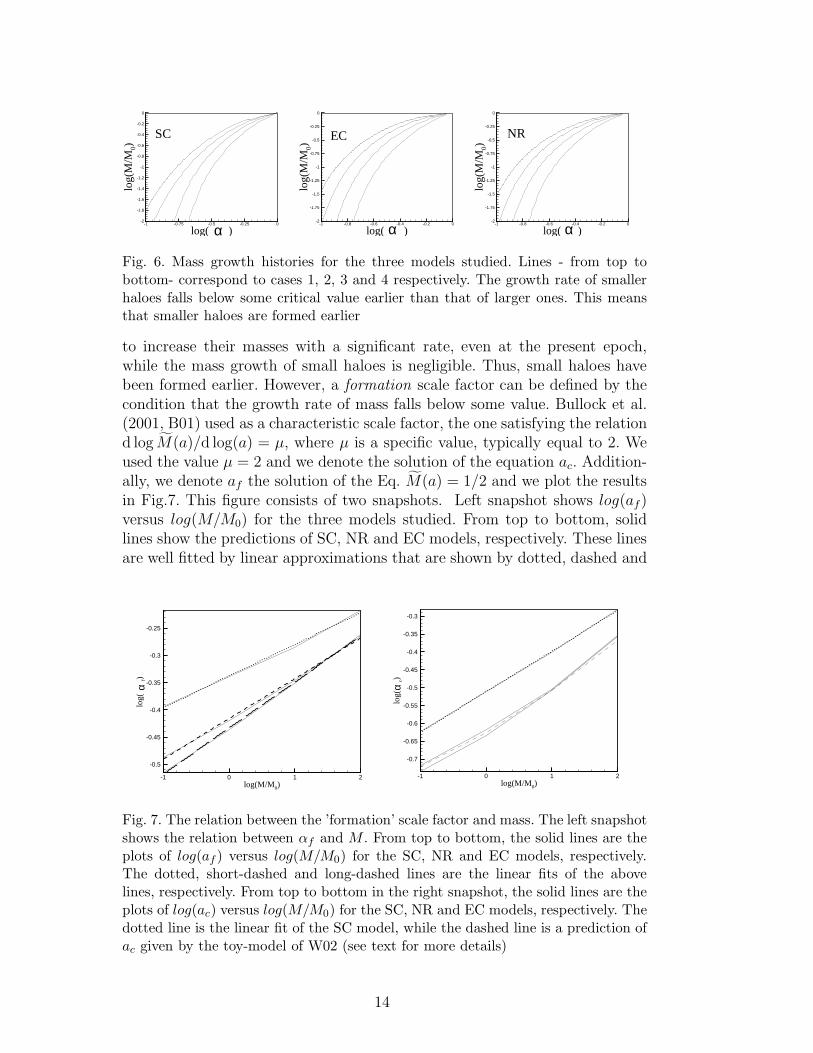
Fig. 6. Mass growth histories for the three models studied. Lines - from top tobottom- correspond to cases 1, 2, 3 and 4 respectively. The growth rate of smallerhaloes falls below some critical value earlier than that of larger ones. This meansthat smaller haloes are formed earlier
to increase their masses with a significant rate, even at the present epoch,while the mass growth of small haloes is negligible. Thus, small haloes havebeen formed earlier. However, a formation scale factor can be defined by thecondition that the growth rate of mass falls below some value. Bullock et al.(2001, B01) used as a characteristic scale factor, the one satisfying the relationd log M(a)/d log(a) = µ, where µ is a specific value, typically equal to 2. Weused the value µ = 2 and we denote the solution of the equation ac. Addition-ally, we denote af the solution of the Eq. M(a) = 1/2 and we plot the resultsin Fig.7. This figure consists of two snapshots. Left snapshot shows log(af)versus log(M/M0) for the three models studied. From top to bottom, solidlines show the predictions of SC, NR and EC models, respectively. These linesare well fitted by linear approximations that are shown by dotted, dashed and
-1 0 1 2log(M/M0)
-0.5
-0.45
-0.4
-0.35
-0.3
-0.25
log(
f)
α
α
-1 0 1 2log(M/M0)
-0.7
-0.65
-0.6
-0.55
-0.5
-0.45
-0.4
-0.35
-0.3
log(
c)α
Fig. 7. The relation between the ’formation’ scale factor and mass. The left snapshotshows the relation between αf and M . From top to bottom, the solid lines are theplots of log(af ) versus log(M/M0) for the SC, NR and EC models, respectively.The dotted, short-dashed and long-dashed lines are the linear fits of the abovelines, respectively. From top to bottom in the right snapshot, the solid lines are theplots of log(ac) versus log(M/M0) for the SC, NR and EC models, respectively. Thedotted line is the linear fit of the SC model, while the dashed line is a prediction ofac given by the toy-model of W02 (see text for more details)
14
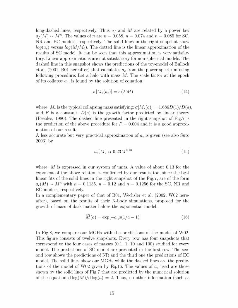
long-dashed lines, respectively. Thus af and M are related by a power lawaf (M) ∼ Mn. The values of n are n = 0.058, n = 0.074 and n = 0.085 for SC,NR and EC models, respectively. The solid lines in the right snapshot showlog(ac) versus log(M/M0). The dotted line is the linear approximation of theresults of SC model. It can be seen that this approximation is very satisfac-tory. Linear approximations are not satisfactory for non-spherical models. Thedashed line in this snapshot shows the predictions of the toy-model of Bullocket al. (2001, B01 hereafter) that calculates ac from the power spectrum usingfollowing procedure: Let a halo with mass M . The scale factor at the epochof its collapse ac, is found by the solution of equation.:
σ[M∗(ac)] = σ(FM) (14)
where,M∗ is the typical collapsing mass satisfying: σ[M∗(a)] = 1.686D(1)/D(a),and F is a constant. D(a) is the growth factor predicted by linear theory(Peebles, 1980). The dashed line presented in the right snapshot of Fig.7 isthe prediction of the above procedure for F = 0.004 and it is a good approxi-mation of our results.A less accurate but very practical approximation of ac is given (see also Suto2003) by
ac(M) ≈ 0.23M0.13 (15)
where, M is expressed in our system of units. A value of about 0.13 for theexponent of the above relation is confirmed by our results too, since the bestlinear fits of the solid lines in the right snapshot of the Fig.7, are of the formac(M) ∼ Mn with n = 0.1135, n = 0.12 and n = 0.1256 for the SC, NR andEC models, respectively.In a complementary paper of that of B01, Wechsler et al. (2002, W02 here-after), based on the results of their N-body simulations, proposed for thegrowth of mass of dark matter haloes the exponential model:
M(a) = exp[−acµ(1/a− 1)] (16)
In Fig.8, we compare our MGHs with the predictions of the model of W02.This figure consists of twelve snapshots. Every row has four snapshots thatcorrespond to the four cases of masses (0.1, 1, 10 and 100) studied for everymodel. The predictions of SC model are presented in the first row. The sec-ond row shows the predictions of NR and the third one the predictions of ECmodel. The solid lines show our MGHs while the dashed lines are the predic-tions of the model of W02 given by Eq.16. The values of ac used are thoseshown by the solid lines of Fig.7 that are predicted by the numerical solutionof the equation d log(M)/d log(a) = 2. Thus, no other information (such as
15
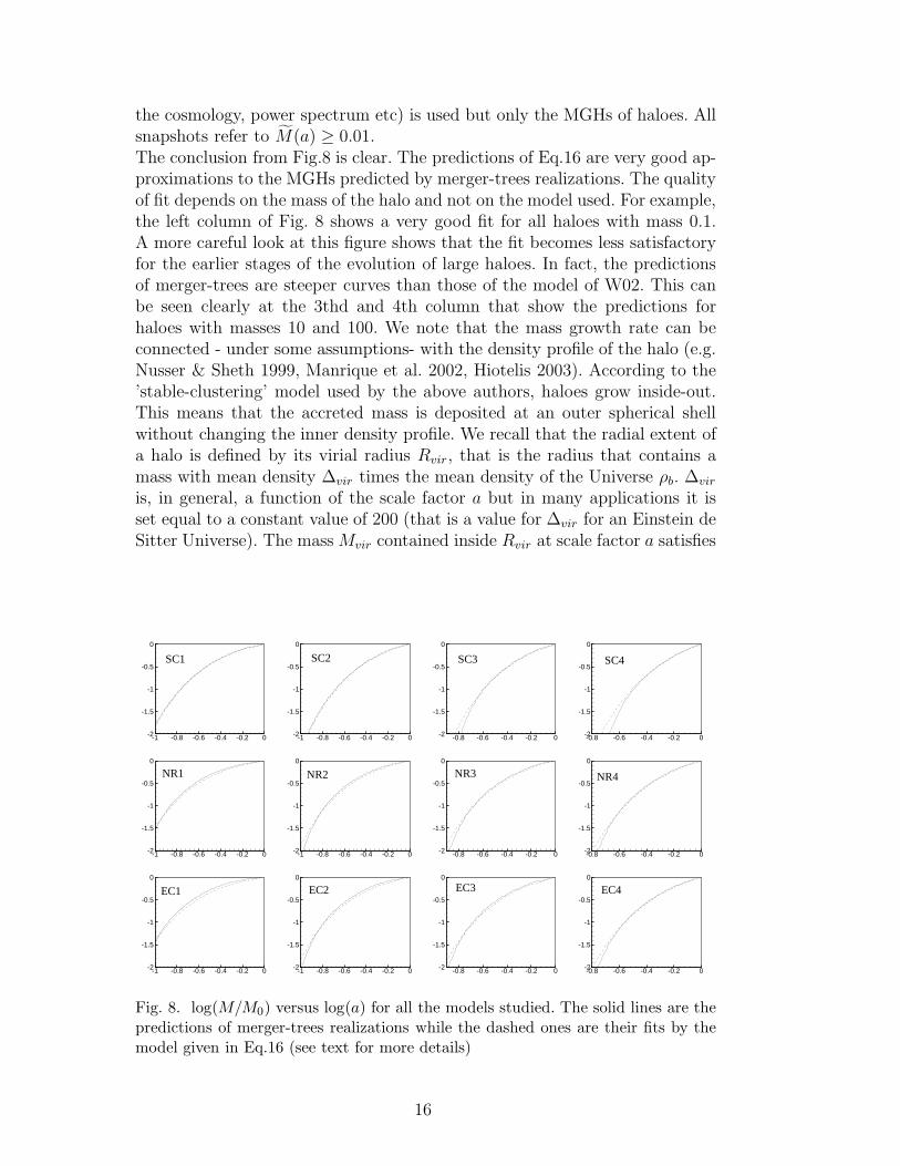
the cosmology, power spectrum etc) is used but only the MGHs of haloes. Allsnapshots refer to M(a) ≥ 0.01.The conclusion from Fig.8 is clear. The predictions of Eq.16 are very good ap-proximations to the MGHs predicted by merger-trees realizations. The qualityof fit depends on the mass of the halo and not on the model used. For example,the left column of Fig. 8 shows a very good fit for all haloes with mass 0.1.A more careful look at this figure shows that the fit becomes less satisfactoryfor the earlier stages of the evolution of large haloes. In fact, the predictionsof merger-trees are steeper curves than those of the model of W02. This canbe seen clearly at the 3thd and 4th column that show the predictions forhaloes with masses 10 and 100. We note that the mass growth rate can beconnected - under some assumptions- with the density profile of the halo (e.g.Nusser & Sheth 1999, Manrique et al. 2002, Hiotelis 2003). According to the’stable-clustering’ model used by the above authors, haloes grow inside-out.This means that the accreted mass is deposited at an outer spherical shellwithout changing the inner density profile. We recall that the radial extent ofa halo is defined by its virial radius Rvir, that is the radius that contains amass with mean density ∆vir times the mean density of the Universe ρb. ∆vir
is, in general, a function of the scale factor a but in many applications it isset equal to a constant value of 200 (that is a value for ∆vir for an Einstein deSitter Universe). The mass Mvir contained inside Rvir at scale factor a satisfies
-1 -0.8 -0.6 -0.4 -0.2 0-2
-1.5
-1
-0.5
0
NR2
-0.8 -0.6 -0.4 -0.2 0-2
-1.5
-1
-0.5
0
NR3
-0.8 -0.6 -0.4 -0.2 0-2
-1.5
-1
-0.5
0
EC4
-0.8 -0.6 -0.4 -0.2 0-2
-1.5
-1
-0.5
0
EC3
-1 -0.8 -0.6 -0.4 -0.2 0-2
-1.5
-1
-0.5
0
EC2
-0.8 -0.6 -0.4 -0.2 0-2
-1.5
-1
-0.5
0
NR4
-0.8 -0.6 -0.4 -0.2 0-2
-1.5
-1
-0.5
0
SC4
-0.8 -0.6 -0.4 -0.2 0-2
-1.5
-1
-0.5
0
SC3
-1 -0.8 -0.6 -0.4 -0.2 0-2
-1.5
-1
-0.5
0
SC2
-1 -0.8 -0.6 -0.4 -0.2 0-2
-1.5
-1
-0.5
0
SC1
-1 -0.8 -0.6 -0.4 -0.2 0-2
-1.5
-1
-0.5
0
NR1
-1 -0.8 -0.6 -0.4 -0.2 0-2
-1.5
-1
-0.5
0
EC1
Fig. 8. log(M/M0) versus log(a) for all the models studied. The solid lines are thepredictions of merger-trees realizations while the dashed ones are their fits by themodel given in Eq.16 (see text for more details)
16
the two following equations:
Mvir(a) = 4π
Rvir(a)∫
0
r2ρ(r)dr (17)
Mvir(a) =4
3π∆vir(a)ρb(a)R
3vir(a) (18)
If the mass history of the halo is known, (that is the evolution of its mass asa function of the scale factor), then the density profile can be calculated bydifferentiating Eq. 17 with respect to a, which gives:
ρ(a) =1
4πR2vir(a)
dMvir(a)
da
(dRvir(a)
da
)−1
(19)
where dRvir(a)/da is calculated by differentiating Eq.18. Finally Eqs. 19 and18 give, in a parametric form, the density profile. It is clear that the densityprofile calculated from the above approximation depends crucially on the massgrowth rate. Hiotelis (2003) used a model based on the above assumptions forhaloes that grow by accretion of matter. This means that the infalling matteris in a form of small haloes (relative to the mass of the growing halo) andthe procedure can be approximated by a continuous infall. In that case, it wasshown that large growth rate of mass (observed in heavy haloes) leads to innerdensity profiles that are steeper than those of less massive haloes (where thegrowth rate of mass is smaller).We recall that the density profile of dark matter haloes is a very difficult prob-lem contaminated by debates between the results of observations, the resultsof numerical simulations and the ones of analytical methods (e.g. Sand et.al 2004 and references therein). Especially the inner density profile seems tofollow a law of the form ρ(r) ∝ r−γ but the value of γ is not still known. Obser-vations estimate a value of γ about 0.52 (Sand et. al 2004), while the resultsof N-body simulations report different values as 1 (Navarro et al. 1997), orbetween 1. and 1.5 (Moore et al. 1998). Additional results from N-body simu-lations, as well as from analytical studies, connect the value of γ with the totalmass of the halo (Ricotti 2002, Reed et al. 2005, Hiotelis 2003). In any case,it is difficult to explain the differences appearing in the results of different ap-proximations. For example, regarding N-body simulations, some of the resultsare effects of force resolution. In a typical N-body code, such as TREECODE(Hernquist 1987) the force acting on a particle is given by the sum of twocomponents: the short-range force that is due to the nearest neighbours andthe long-range forces calculated by an expansion of the gravitational potentialof the entire system. As it can be shown, the value of the average stochasticforce in the simulation is an order of magnitude greater than that obtainedby the theory of stochastic forces. Consequently, small fluctuations induced
17
by the small-scale substructure are not ’seen’. This is the case of cold darkmatter models in which the stochastic force generators are substructures atleast three orders of magnitude smaller in size than the protoclusters in whichthey are embedded (e.g. clusters of galaxies). On the other hand, regardingthe differences between the results of various approximations, we notice thatsome of these differences could be due to the presence of the baryonic mat-ter. Especially in regions, as the central regions of haloes, the large density ofbaryonic matter may affect the distribution of dark matter.Since in this paper we describe in detail technical problems related to the con-struction of reliable merger-trees, we have to note that the inside-out model forthe formation of haloes described above, requires calculations for very smallvalues of a, because the central regions are formed earlier. Therefore, in orderto explore the center of the halo we have to go deep in the past of its history.Consequently, the problems relative to the calculation of mean mass that an-alyzed at the beginning of this section, become more difficult. The densityprofiles predicted by the above described approximation are under study.
5 Discussion
Analytical models based on the extended PS formalism provide a very usefultool for studying the merging histories of dark matter haloes. Comparisonswith the results of high resolution numerical simulations or observations showthat the predictions of EPS models are satisfactory (e.g. Lin et al. 2003, Ya-hagi et al. 2004, Cimatti et al. 2002, Fontana et. al 2004), although differencesbetween various approximations always exist. These differences show the needfor further improvement of various methods.In this paper we described in detail the numerical algorithm for the construc-tion of merger-trees. The construction is based on the mass-weighted proba-bility relation that is connected to the model barrier. The choice of the barrieris crucial for a good agreement between the results obtained by merger-treesand those of N-body simulations. As it is shown in Yahagi et al. (2004) massfunctions resulting from the SC model are far from the results of N-body sim-ulations while those predicted by non-spherical models are in good agreement.Our results show that the distributions of formation times predicted by thenon-spherical models are shifted to smaller values. Thus, the resulting forma-tion times are closer to the results of N-body simulations than the formationtimes predicted by the SC model. It should be noted that N-body simulationsgive, in general, smaller formation times than that of EPS models (e.g. Lin etal. 2003). It should also be noted that observations indicate a build-up of mas-sive early-type galaxies in the early Universe even faster than that expectedfrom simulations (Cimatti, 2004).We have shown that a small sample of haloes (≥ 1000) is sufficient for the
18
prediction of smooth mass growth histories. These curves have a functionalform that is in agreement with those proposed by the N-body results of otherauthors. In particular the set of relations:
ac(M0) = 0.24M0.120 (20)
and
M(a)/M0 = exp[−2ac(M0)(1/a− 1)] (21)
describes very satisfactorily the results of non-spherical models (NR and EC).These relations give the mass M of dark matter haloes at scale factor a forthe range of mass described in the text and for the particular cosmology used.M0 is the present day mass of the halo in units of 1012h−1M⊙.Finally, it should be noted that a large number of questions regarding theformation and evolution of galaxies remains open. For example, a first stepshould be the improvement of the model barrier so that the results of merger-trees fit better both the mass function (Yahagi et al. 2004) and the collapsescale factor (Lin et al. 2003). It should be noted also that structures appearto form earlier in N-body simulations and even earlier in real Universe. Ad-ditionally, predictions relative to the density profile are of interest. Some ofthese issues are currently under study.
6 Acknowledgements
We are grateful to the anonymous referee for helpful and constructive com-ments and suggestions. N. Hiotelis acknowledges the Empirikion Foundation
for its financial support and Dr M. Vlachogiannis for assistance in manuscriptpreparation.
References
[1991] Bond, J.R., Cole, S., Efstathiou, G., Kaiser, N., 1991, ApJ, 379, 440(1991ApJ...379..440B)
[1991] Bower, R., 1991, MNRAS, 248, 332 (1991MNRAS.248..332B)
[2001] Bullock, J. S., Kolatt, T. S., Sigad, Y., Somerville, R. S., Kravtsov,A.V., Klypin, A. A., Primack, J. R., Dekel, A., 2001, MNRAS, 321, 559(2001MNRAS.321..559B)
19
[1998] Catelan, P., Lucchin, F. Matarrese, S., Porciani, C., 1998, MNRAS, 297, 692(1998MNRAS.297..692C)
[2004] Cimatti A., Daddi,E., Renzini,A., Cassata,P., Vanzella,E., Pozzetti,L.,Cristiani,S., Fontana,A., Rodighiero,G., Mignoli,M., Zamorani,G., 2004, Nature,430,184. (2004Natur.430..184C)
[2002] Cimatti A., Daddi,E., Mignoli,M.,Pozzetti,L.,Renzini,A., Zamorani,G.,Broadhurst,T.,Fontana,A., Saracco,P.,Poli,F., Cristiani,S.,D’Odorico,S.,Giallongo,E.,Gilmozzi,R.,Menci,N., 2002, A&A,381, L68 (2002A&A...381L..68C)
[1998] Del Popolo, A., Gambera, M., 1998, A&A, 337, 96 (1998A&A...337...96D)
[2004] Fontana, A., Pozzetti, L., Donnarumma, I., Renzini,A., Cimatti, A.,Zamorani, G., Menci,N., Daddi, E., Giallongo, E., Mignoli,M., Perna, C.,Salimbeni, S., Saracco,P., Broadhurst,T., Cristiani,S., D’Odorico,S., Gilmozzi,R.,2004, A&A, 424, 23 (2004A&A...424...23F)
[1987] Hernquist L., 1987, ApJS, 64, 715 (1987ApJS...64..715H)
[2003] Hiotelis, N., 2003, MNRAS, 344,149 (2003MNRAS.344..149H)
[2001] Jenkins ,A., Frenk, C.S., White, S.D.M., Colberg, J.M., Cole, S.,Evrard, A.E., Couchman, H.P.M., Yoshida, N., 2001, MNRAS, 321, 372(2001MNRAS.321..372J)
[1993] Lacey, C., Cole, S., 1993, MNRAS, 262, 627 (1993MNRAS.262..627L)
[2003] Lin, W.P., Jing, Y.P., Lin, L., 2003, MNRAS, 344, 1327(2003MNRAS.344.1327L)
[2003] Manrique A., Raig A., Salvador-Sole E., Sanchis T., Solanes J.M., 2003, ApJ,593, 26 (2003ApJ...593...26M)
[1996] Mo, H.J., White, S.D.M., 1996, MNRAS, 282, 347 (1996MNRAS.282..347M)
[1998] Moore, B., Governato, F., Quinn, T., Stadel, J., Lake, G., 1998, ApJ, 499,L5(1998ApJ...499L...5M )
[1997] Navarro, J., Frenk, C.S., White S.D.M., 1997, ApJ, 490, 493(1997ApJ...490..493N)
[1999] Nusser, A., Sheth, R.K., 1999, MNRAS, 303, 685 (1999MNRAS.303..685N )
[1980] Peebles P.J.E., 1980, The Large-Scale Structure of the Universe, PrincetonUniv. Press, Princeton, NJ (1980lssu.book.....P)
[1974] Press W., Schechter P., 1974, ApJ, 187, 425 (1974ApJ...187..425P)
[1990] Press W.H., Flannery B.P., Teukolsky, S.A., Vetterling, W.T., 1990,Numerical Recipes, Cambridge University Press ()
[2005] Reed D., Governato, F., Verde, L., Gardner, J., Quinn, T., Stadel, J., Merritt,D., Lake, G., 2005, MNRAS, 357, 82 (2005MNRAS.357...82R)
20
[2003] Ricotti M. 2003, MNRAS, 344, 1237 (2003MNRAS.344.1237R)
[2004] Sand D.J., Treu T., Smith G.P., Ellis R.S., 2004, ApJ, 604, 88(2004ApJ...604...88S)
[1999] Sheth, R.K., Lemson G., 1999a, MNRAS, 304, 767 (1999MNRAS.304..767S)
[1999] Sheth, R.K., Lemson G., 1999b, MNRAS, 305, 946 (1999MNRAS.305..946S)
[1999] Sheth, R.K., Tormen G., 1999, MNRAS, 308, 119 (1999MNRAS.308..119S)
[2002] Sheth, R.K., Tormen G., 2002, MNRAS, 329, 61 (2002MNRAS.329...61S)
[1998] Smith, C.C., Klypin, A., Gross, M.A.K., Primack, J.R., Holtzman, J., 1998,MNRAS, 297, 910 (1998MNRAS.297..910S)
[1999] Somerville, R.S., Kollat, T.S., 1999, MNRAS, 305, 1 (1999MNRAS.305....1S)
[2003] Suto, Y., 2003, Density profiles and clustering of dark halos and clusters ofgalaxies, In ”Matter and Energy in Clusters of galaxies”, ASP Conference Series,Vol.301, 379, 2003, Eds.: S. Bowyer and C.-Y.Hwang (2003mecg.conf..379S)
[2004] Yahagi, H., Nagashima, M., Yoshii, Y., 2004, ApJ, 605, 709(2004ApJ...605..709Y)
[2002] van den Bosch, F.G., 2002, MNRAS, 331, 98 (2002MNRAS.331...98V)
[2002] Wechsler, R.H., Bullock, J.S., Primack, J.R., Kratsov, A.V., Dekel, A., 2002,ApJ, 568, 52 (2002ApJ...568...52W)
21