Market Closure and Short-Term Reversal∗

Pasquale Della Corte Robert Kosowski Tianyu Wang

This version is incomplete, please do not distribute

This Version: November 2015

∗The authors would like to thank Franklin Allen, Marcin Kacperczyk, Dong Lou, Lubos Pastor, seminarparticipants at Oxford-Man Institute of Quantitative Finance and 10th Annual Conference on Advances in theAnalysis of Hedge Fund Strategies for comments and helpful discussions. Pasquale Della Corte is with ImperialCollege London and the Centre for Economic Policy Research (CEPR), email: p.dellacorte@imperial.ac.uk.Robert Kosowski is with Imperial College London and the Centre for Economic Policy Research (CEPR), email:r.kososki@imperial.ac.uk. Tianyu Wang is with Imperial College London, email: t.wang12@imperial.ac.uk.

Market Closure and Short-Term Reversal

Abstract

A strategy that holds daily long and short positions, respectively, in assets with low and

high past overnight returns – overnight-intraday reversal strategy - generates for the US stock

market an average excess return that is five times larger when compared to a conventional

short-term reversal strategy. Our results remain robust to using international stocks as well as

equity index, interest rate, commodity, and currency futures. We find that overnight-intraday

reversals are consistent with the simulated patterns generated by the continuous-time model

with periodic market closures of Hong and Wang (2000). Finally, we demonstrate that only

intraday returns matter for the reversal-based liquidity measure of Pastor and Stambaugh

(2003).

Keywords: Short-term reversal, Liquidity, Market closure

JEL Classification: G11, G12, G15, G20

1 Introduction

Financial markets are typically closed overnight and during a weekend. These periodic closures

affect trading conditions as non-trading hours are characterized by low trading activity and low

liquidity (Barclay and Hendershott, 2003, 2004). Among the several anomalies, a short-term

reversal strategy that buys past loser and sells past winner stocks (Jegadeesh, 1990; Lehmann,

1990), is theoretically and empirically linked to liquidity (Grossman and Miller, 1988; Campbell,

Grossman, and Wang, 1993; Avramov, Chordia, and Goyal, 2006), and the return of this strategy

is used as a proxy for profit from liquidity provision (Nagel, 2012). The different liquidity con-

ditions in these two periods highlight the necessity of investigating the effects of market closures

on short-term reversal.

The short-term reversal strategy has been explored at various frequencies: daily, weekly and

monthly.1 The failure of the monthly short-term reversal strategy to deliver positive return in

stock market in recent decade coincides with market technology advancement and market mi-

crostructure development, and it also indicates improved liquidity provision activity. Hendershott

and Menkveld (2014) measure the price pressures induced by risk-averse market makers supply-

ing liquidity to asynchronously arriving investors. They show that based on New York Stock

Exchange data, the price pressure is 0.49% on average with a half life of 0.92 days. In addition,

the liquidity measure of Pastor and Stambaugh (2003) relies on the daily reversals. Therefore,

analysing short-term reversal in daily, even in intra-daily frequency allows to better capture the

liquidity effect.

In addition, the reversal strategy has been widely examined in United States, but there is

little or no research on international stock, equity index, interest rate, commodity and currency

markets. The extension of the analysis to international stock markets and other asset classes is of

interest for several reasons. On one hand, it provides robustness test to the empirical findings and

theoretical models in United States, especially in more recent and liquid stock samples. On the

other hand, the analysis of short-term reversal on very liquid markets (equity index, interest rate,

commodity and currency futures markets) provides useful insights for the research on liquidity.

The theoretical motivation of short-term reversal is from Grossman and Miller (1988) in which

1There is a broad literature that documents short-term reversal effects using monthly (e.g., Jegadeesh, 1990;Da, Liu, and Schaumburg, 2013; Hameed and Mian, 2015), weekly (e.g., Jegadeesh, 1990; Avramov, Chordia, andGoyal, 2006), and daily (e.g., Nagel, 2012; So and Wang, 2014; Collin-Dufresne and Daniel, 2013) returns.

1

risk-averse market makers demand compensation for providing liquidity. They also discuss differ-

ent market structures of futures market and stock market, and the high demand for immediacy

of futures market causes the market to be designed to supply maximal immediacy of order exe-

cution, especially at the open. Therefore, the illiquidity effect, measured by short-term reversal,

is absent or trivial in futures market. Based on the model of Kyle (1985) and Grossman and

Miller (1988), Nagel (2012) shows that the short-term reversal strategy is highly predictable by

the VIX index, which is commonly used to measure the market-wide uncertainty level. Financial

intermediaries’ activities are limited and constrained when the market volatility is high (Gromb

and Vayanos, 2002; Brunnermeier and Pedersen, 2009; Adrian and Shin, 2010), so the liquidity

provision is limited.

The market opens and closes are the most specific points in the intra-daily periods. Ami-

hud and Mendelson (1987) document that open-to-open returns have higher variance and more

negative serial autocorrelation than close-to-close returns, which result from different trading

mechanisms at the open and close. Consistent with the literature, we denote the trading hours as

the intraday period and the non-trading hours as the overnight period2. Stoll and Whaley (1990)

find a high negative overnight-intraday serial autocorrelation and argues that it indicates a high

profit of liquidity provision at the open. We extend the work by Stoll and Whaley (1990) to

check the economic value of the negative serial autocorrelation, and show it measures more than

the implied bid-ask spread. Furthermore, the issue of errors in open prices in Stoll and Whaley

(1990) is mitigated in our paper, since we use samples in more recent period and also analyze

subsample of large and liquid stocks (for instance, S&P100 stocks) or futures data.

The market open3 is the time of interest, since liquidity provision is more likely to happen

during trading hours, while the time after close typically with little (stock markets) or no (futures

markets) trading volume. The market open has the highest uncertainty level measured by the

realized volatility as in Barclay and Hendershott (2003), and also by the VIX index level shown

in this paper, which a forward-looking measure. The high volatility at the open potentially re-

sults from information asymmetry or high informationless trading shocks. The high asymmetric

2In weekly frequency, the intraday period is the weekday, and the overnight period is the weekend.3A lot of papers have examined the microstructure issues at market open and the preopening time. However,

the microstructure of the stock and other asset markets are quite different, for instance, as discussed by Grossmanand Miller (1988) for futures and stock. We only focus on the most common features: the open and close of themarkets, and the high uncertainty at the open.

2

information in pre-open period may also exaggerates the price impact induced by adverse se-

lection problem. However, the price impact of private information is permanent and does not

induce short-term reversal (Glosten and Milgrom, 1985), which instead captures the transitory

component. Due to the high uncertainty level, the downward-sloping demand curves become

steep for the increasing inventory risks faced by the market makers at the open, thus the liquid-

ity provisions ask for high compensation. Focusing on the open time at the expiration days of

index futures contracts, when there are large order imbalances in the underlying stocks caused by

largely informationless liquidity shocks, Barclay, Hendershott, and Jones (2008) show that there

are large excess volatility and overnight-intraday reversal.

The market opens and closes are perfectly anticipated and repeated events, which will affect

short-term reversals. So and Wang (2014) study short-term reversal during earning announce-

ments and find that market makers demand high compensation prior to announcements because

of the increasing inventory risks that induced by the uncertainty of anticipated information event.

Lou, Yan, and Zhang (2013) show that Treasury security prices in the secondary markets signif-

icantly decrease before Treasury auctions and recover thereafter, even though these events are

perfectly anticipated. They confirm that the dealers’ limited risk-bearing capacity and the im-

perfect capital mobility explain the reversal in this very liquid market. In this paper, instead

of focusing only on the earning/auction announcement window, we show that it is a story that

repeated in daily frequency. The general market makers anticipate high uncertainty level during

the open, which implies high inventory risks of holding stocks.

Our findings can be summarized as follows. Firstly, in US stock market, both the return and

Sharpe ratio of the reversal strategy that takes into account the different conditions in trading

and non-trading hours (overnight-intraday reversal, denoted as CO-OC strategy thereafter) are

on average five times in magnitude of the conventional reversal strategy, and the pattern is

consistently present over time. In addition, the short-term reversal strategy achieves better

performance based on open-to-open returns than close-to-close returns, which is consistent with

the serial autocorrelation tests in Amihud and Mendelson (1987). Using the autocorrelation

regression, we find that the 39% (25%) of the overnight return will reverse in the later (first)

intraday periods, while the number for intraday return is only 2%.

Secondly, we document that a similar short-term reversal effect exists across international

3

stock, equity index, interest rate, commodity and currency markets. This result is novel to the

best of our knowledge. On one hand, international stock markets have the same pattern of short-

term reversal as in US stock market. On the other hand, we find no evidence of short-term reversal

of the conventional strategy from the interest rate, commodity and currency markets, consistent

with the arguments in Grossman and Miller (1988). Specifically, in commodity market, there is

a clear signal of daily momentum (Baltas and Kosowski, 2011), instead of short-term reversal.

In contrast, the CO-OC strategy delivers positive and significant returns across all of these asset

classes, and outperforms the other three short-term reversal strategies, both in daily and weekly

frequency.

Thirdly, extending the analysis in Nagel (2012), we find that the increment of the uncertainty

during the non-trading hours (change of VIX from the last close to open) adds explanatory power

for the returns of CO-OC strategies in different equity markets and other asset classes, aside from

the uncertainty at the market close. Besides, we empirically confirm that the VIX level at the

open is significantly higher than any other time, the average VIX level is 20.37 around the market

open window, while the average level is 20.21 in other time, and the difference is significant with

a Newey-West adjusted t-statistic of 5.42, based on the sample from January 1993 to December

2013.

Fourthly, based on the continuous-time model with periodic market closures in Hong and

Wang (2000), we show that overnight-intraday reversal pattern is consistent with an equilibrium

in a market periodically closed. In the model, the investors have periodic trading behaviors due

to the exogenous market closures. The two investors use stock to hedge their private investment

opportunities4, which have correlated payoffs with stock. In equilibrium, the investors’ optimal

hedging demands are time-varying, due to the anticipated market open and close. The stock price

has higher exposure to the liquidity shocks at the open than at the close, since the investors could

trade stock to hedge the private investment after the open, when the accumulated trading demand

during the closure period is released. The higher exposure to the private investment at the open

induces higher return variance. Based on the simulated results, we confirm that the empirical

results are consistent with the model’s implication. In addition, changing the parameters related

to liquidity shocks supports the predication that the hedging demands induce overnight-intraday

4This specification of the model allows for generating the hedging demand of the investors.

4

reversals.

Lastly, the diverse patterns of overnight and intraday returns have implications for the

reversal-based market liquidity measure in Pastor and Stambaugh (2003). Following the steps

in their paper, we form the tradable long-short portfolios based on the stocks’ exposure to the

historical liquidity measures. The tradable factor based on intraday return liquidity measure cap-

tures the return of the original Pastor and Stambaugh (2003) liquidity factor, while the overnight

part shows insignificant return. For the market liquidity measure, the intraday return element is

the important component. The overnight-intraday reversal is more likely induced by firm specific

liquidity characteristics.

Literature

In addition to the literature mentioned above, our paper is related to the broad researches that

explore short-term reversal in stock market. Jegadeesh and Titman (1995) show that the pattern

of short-term negative serial autocorrelation for stock returns is consistent with the implications of

inventory-based microstructure models. Empirically, Conrad, Hameed, and Niden (1994) provide

supportive evidence that market-adjusted return reversals are stronger for stocks that experience

a large increase in volume in a sample of NASDAQ stocks. Conrad, Gultekin, and Kaul (1997)

suggest that much of the reversal profitability is within the bid-ask bounce.

More recently, Hameed and Mian (2015) document pervasive evidence of intra-industry re-

versal in monthly returns, and intra-industry reversal is larger in magnitude than conventional

reversal strategy and persistent over time. Da, Liu, and Schaumburg (2013) show that stock

returns unexplained by “fundamentals”, such as cash flow news, are more likely to reverse in the

short-term than those linked to fundamental information.

Through decomposing the daily return into overnight and intraday returns, Lou, Polk, and

Skouras (2015) show that all of the abnormal returns on momentum strategy occur during the

non-trading period, while other anomalies’ returns are accumulated during the trading period. In

monthly frequency, they also show a long-short portfolio in the past one month overnight returns

has a three-factor overnight alpha of 3.47% per month and a three-factor intraday alpha of -3.02%

per month. We differ from them in several aspects. Firstly, using daily and weekly frequency

allows better understanding of the short term reversal effects. Secondly, we provide similarly

5

short-term reversal patterns comprehensively across international stock markets and other asset

classes. Based on 48,000 stocks from 35 countries including US, Aretz and Bartram (2015) extend

the work of Lou, Polk, and Skouras (2015), and show that most well-known anomalies, including

momentum, have positive returns over the trading period.

Our work also relates to the recent studies on global asset pricing. Fama and French (2012)

study the returns to size, value, and momentum in individual stocks across global equity markets

and find consistent risk premia across different markets. Koijen, Moskowitz, Pedersen, and Vrugt

(2013) document global “carry” returns, which predict returns both in the cross section and time

series for a variety of different asset classes including global equities, global bonds, commodities,

US Treasuries, credit, and options. Moskowitz, Ooi, and Pedersen (2012) demonstrate global

evidence of time series momentum strategy that using each asset’s own past returns. Time

series momentum is significantly different from the cross-sectional momentum strategies. Asness,

Moskowitz, and Pedersen (2013) find consistent value and momentum return premia across eight

diverse markets and asset classes, and present a common factor structure among their returns.

2 Data and Methodology

This section describes the data on international stock markets as well as futures contracts on

different asset classes employed in our empirical analysis. We also summarize the data on exchange

traded funds and volatility indices used as robustness checks. Finally, we define a short-term

reversal strategy that uses overnight (or close-to-open) returns as formation period returns and

the next following intraday (or open-to-close) returns as trading period returns, and compare it

to a variety of alternative short-term reversal strategies based on different combinations of open

and close prices. We will provide a statistical and an economic evaluation of these strategies in

the next section.

International Stocks. We collect daily open and close prices ranging from January 1993

to December 2014 for the following stock markets: the US, continental Europe (France and

Germany), Japan and the UK. The universe of US stock consists of all common equities in CRSP

with share codes 10 and 11. We only select firms for which the open price is available. In order

to mitigate microstructure issues, we exclude stocks with a share price below $5 as well as stocks

6

whose market capitalization falls within the bottom 5%. For the remaining countries, we source

daily open and close prices from Datastream and employ the same filtering rules applied to US

stocks.

As a robustness check, we also collect the best bid and offer quotes at the open and minute

level trade prices from Trade and Quote (TAQ) database from January 2011 to December 2014

for a subsample of US stocks.

Futures Contracts. We obtain from TickData daily open and close prices on 35 futures

contracts traded on Chicago Mercantile Exchange. The sample ranges from July 1982 to De-

cember 20145 and consists of futures written on 5 equity indices (DJIA, NASDAQ, NIKKEI

225, S&P400 and S&P500), 11 interest rates (30-day Federal Funds, Eurodollar CME, LIBOR

1-month, Municipal Bonds, T-Bills, 5-year Interest Rate Swap, US 2-year T-Note, US 5-year

T-Note, US 10-year T-Note, US 30-year T-Bond, and Ultra T-Bond), 11 commodities (Corn,

Ethanol CBOT, Lumber, Live Cattle, Lean Hogs, Oats, Pork Bellies, Rough Rice, Soybean Meal,

Soybeans, Wheat CBOT) and 9 currencies (Australian dollar, British pound, Canadian dollar,

Deutsche mark, euro, Japanese yen, Mexican peso, New Zealand dollar and Swiss franc vis-a-vis

the US dollar). For each contract, we always select the most liquid contract as in De Roon,

Nijman, and Veld (2000) and Moskowitz, Ooi, and Pedersen (2012). The most liquid contract

is generally the nearest-to-delivery (front) contract, when the second-to-delivery (first-back) con-

tract becomes the most liquid one and a rollover takes place.6

Exchange Traded Funds. We collect daily open and close prices on equity index, govern-

ment bond, commodity and currency exchange traded funds (ETF) from March 1999 to December

2014. ETFs on equity indices (identified by the following tickers: IVV, IJH, IWB, IWM, IWV,

OEF, and QQQ), government bonds (AGZ, GOVT, IEF, IEI, SHV, SHY, STIP, TFLO, TLH,

TLT, TIP), commodities (CMDT, COMT, FILL, GSG, IAU, PICK, RING, SLV, SLVP, VEGI)

and currencies (DBV, EUO, FXA, FXC, FXE, FXF, FXY, USDU, UUP, YCS) from CRSP. For

the first three asset classes, we use ETFs issued by iShares except QQQ. For the currency ETFs,

we select funds with assets under management higher than $100 millions from various providers.

5Not all futures contracts start from July 1982.6Our findings are robust to using front contracts and futures contracts in other international exchanges. Results

are available upon request.

7

Volatility Index and Futures. We obtain data on volatility indices from Chicago Board

Options Exchange. The sample consists of the S&P500 volatility index (VIX), S&P100 volatility

index (VXO), NASDAQ volatility index (VXN) and the DJIA volatility index (VXD). From the

same source, we also collect open and close prices for VIX futures contracts. The EURO STOXX

50 volatility (VSTOXX), Nikkei stock average volatility index (VNKY) and FTSE 100 implied

volatility index (IVI) are from Bloomberg.

Short-term reversal strategy. We construct our short-term reversal strategy as in Lehmann

(1990), Jegadeesh and Titman (1995) and Nagel (2012). We consider a zero-investment portfolio

strategy where the portfolio weight on asset i at time t− 1 is given by

wi,t−1 = − 1

N(ri,t−1 − rt−1) (1)

where ri,t−1 denotes the discrete return on the asset i at time t − 1, rt−1 = N−1∑N

i=1 ri,t−1 is

the equally-weighted average return on all assets N available at time t − 1. This strategy is

by construction a contrarian strategy as it sells past winners and buys past losers, and is zero-

investment strategy as∑N

i=1wi,t−1 = 0. The portfolio returns are then computed assuming a

50% margin position as in Lehmann (1990) and Nagel (2012)

rp,t =πt

dt−1/2. (2)

where πt =∑N

i=1wi,t−1ri,t denotes the accounting profits at time t and dt−1 =∑N

i=1 |wi,t−1| is

the total amount of dollars invested in both long and short positions at time t− 1.

The traditional short-term reversal strategy uses the underlying assets’ close-to-close daily

returns on day t−1 as long/short signals. The portfolio return is then realized on the subsequent

business day using the underlying assets’ close-to-close daily returns on day t. The short-term

reversal strategy studied in this paper differently uses overnight returns as signals and then

realizes the following intraday returns. To clarify our notation, let P oi,t and P ci,t denote the open

and close prices for asset i on day t, respectively. The close-to-close daily return on day t is

defined as

rcci,t =P ci,tP ci,t−1

− 1. (3)

8

that is decomposed into close-to-open (or overnight) daily return

rcoi,t =P oi,tP ci,t−1

− 1 (4)

and open-to-close (or intraday) daily return

roci,t =P ci,tP oi,t− 1. (5)

such that rcci,t ≈ rcoi,t+ roci,t. The traditional short-term reversal strategy uses rcci,t−1 for the portfolio

weights in Equation (1) and rcci,t for the portfolio return in Equation (2). Our short-term reversal

strategy, instead, uses rcoi,t for the portfolio weights in Equation (1) and roci,t for the portfolio

return in Equation (2). We refer to the former as CC-CC strategy and the latter as CO-OC

strategy (i.e., the first two letters define the formation period return whereas the last two letters

indicate the trading period return). We also consider two alternative specifications as robustness:

a strategy labeled as OC-OC that uses roci,t−1 for the portfolio weights and roci,t for the portfolio

return, and a strategy identified as OO-OO that employs rooi,t−1 for the portfolio weights and rooi,t

for the portfolio return with rooi,t = (P oi,t/Poi,t−1) − 1 indicating the open-to-open daily return on

day t. In sum, the empirical analysis will make use of four different short-term reversal strategies

characterized by different formation and trading period returns.7 We summarize these strategies

in Table 1.

3 Empirical Evidence on Short-term Reversal Strategies

This section presents the empirical evidence on four different short-term reversal strategies im-

plemented using international stock returns as well as returns on equity index, interest rate,

commodity and currency futures. We complement our core analysis with a battery of robustness

exercises.

7We do not present results for (i) a purely overnight reversal strategy that uses close-to-open returns on dayt− 1 as trading signals and close-to-open returns on day t as trading period returns, and (ii) an intraday-overnightreversal strategy that uses open-to-close returns on day t− 1 as trading signals and close-to-open returns on day tas trading period returns. These strategies would require to trade overnight when liquidity is tiny and transactioncosts are fairly prohibitive.

9

International Equities. We form the short-term reversal strategies described in Table 1

using international stock market returns and present them in Table 2. The top right panel of

this table shows the empirical evidence for the United States. Recall that a short-term reversal

strategy takes advantage of the tendency of assets with strong losses and assets with strong gains

to reverse in a short interval, typically up to one day or one week. An investor would typically

buy past losers and sell past winners using close-to-close returns on day t − 1 as signals, and

then realize the profit (loss) on the next following day using close-to-close returns on day t. This

traditional strategy which we refer to as CC-CC produces a statistically significant average return

of 0.33% per day (with a t-statistic of 16.57) for the United States, in line with the 0.3% per day

reported in Nagel (2012). A related version of this strategy – labeled as OO-OO – employs open-

to-open returns as opposed to close-to-close returns and generates a similar but more pronounced

pattern since the average return is 0.63% per day (with a t-statistic of 28.09) and the annualized

Sharpe ratio is 9.96, close to double the Sharpe ratio of 5.52 granted by the CC-CC strategy.

Both variants of the short-term reversal strategy discussed above implicitly aggregate overnight

and intraday information. Furthermore, we decompose the overall (or close-to-close) daily return

into an overnight (or close-to-open) and intraday (or open-to-close) return and study whether

short-term reversal strategies are different with these returns. To this end, we first examine a

purely intraday reversal strategy that uses intraday (or open-to-close) returns on day t − 1 as

trading signals and the next following intraday returns (i.e., open-to-close returns on day t) for

the realization of the trading gain. This strategy, defined as OC-OC, displays a negative returns

of −0.17% per day (with a t-statistic of −14.65) and suggests the presence of a fairly strong in-

traday momentum effect. We then examine a naive overnight-intraday reversal strategy that uses

information accumulated overnight as trading signals (i.e., buying overnight losers and selling

overnight winners) and the next following intraday returns for the accounting profit. The former

set of returns are measured at the beginning of day t using close-to-open returns whereas the

latter set of returns are observed at the end of day t using open-to-close returns. This strategy,

identified as CO-OC, earns a large average return that is about 1.68% per day (with a t-statistic

of 46.52). As a comparison, recall that the CRSP value-weighted index for the same sample

period generates a mean return of 0.04% per day with a standard deviation of 1.16%. Overall,

the overnight-intraday reversal strategy exhibits roughly the same volatility as the traditional

10

short-term CC-CC strategy but a way larger return; this translates into a Sharpe ratio of 24.16

that almost five times larger.

It is worth to notice that all short-term reversal strategies display positive skewness thus

implying that downside or crash risk is not a plausible explanation. In particular, the overnight-

intraday CO-OC strategy presents positive returns within the 5th-95th percentile range. We

also find that returns exhibit strong and persistent serial correlation, especially for the CO-OC

strategy, which implies that there are potential high fixed costs (for instance, bid-ask spread)

embedded in the returns. Finally, the overnight-intraday reversal strategy is fairly uncorrelated

with the traditional short-term reversal strategies as its sample correlation evolves around 25%.

Turning to other stock markets, the empirical evidence reveals that the traditional CC-CC

reversal strategy displays sizeable returns for both Continental Europe (0.23% per day with a

Sharpe ratio of 4.02) and Japan (0.26% per day with a Sharpe ratio of 4.55) but generates

negative returns for stocks traded in London (−0.24% per day with a Sharpe ratio of −3.30). The

purely intraday return short-term reversal strategy OC-OC produces negative returns for stocks

traded in Continental Europe (−0.21% per day with a Sharpe ratio of −4.63) and the United

Kingdom (−0.66% per day with a Sharpe ratio of −9.67) but positive returns for stocks traded in

Tokyo (0.04% per day with a Sharpe ratio of 0.70). These results, taken together, reveal mixed

evidence for both traditional short-term reversal strategies and intraday momentum patterns. The

overnight-intraday reversal strategy, instead, is characterized by a large and positive profitability

in all stock markets: the return is about 1.02% per day with a Sharpe ratio of 16.79 in Continental

Europe, 0.74% per day with a Sharpe ratio of 16.25 in Japan, and 1.94% per day with a Sharpe

ratio of 17.41 in the United Kingdom.

Exchange traded futures. In addition to using international stock markets, we also examine

the profitability of short-term reversal strategies for exchange traded futures on equity indices,

interest rates, commodities and currencies. These results are reported in Table 3. The summary

statistics for short-term reversal strategies implemented using equity index futures are reported

in top right panel and remain fairly comparable with the previous table. The result for traditional

CC-CC strategy as expected is both economically and statistically significant since it earns an

average return of 0.08% per day (with a t-statistic of 5.20) and an annualized Sharpe ratio of

1.15. The OO-OO strategy tends to perform better as it yields an average return of 0.20%

11

per day (with a t-statistic of 9.36) and an annualized Sharpe ratio of 2.43. The profitability of

these conventional strategies, however, is largely outperformed by the overnight-intraday reversal

strategy which delivers an average return of 0.25% per day (with a t-statistic of 13.18) and an

annualized Sharpe ratio of 4.08. Yet, its sample correlation with the other three strategies remain

extremely low, ranging from 1% to 4%.

For futures contracts written on other asset classes, the traditional short-term reversal strat-

egy CC-CC produces either negative returns (interest rate and commodity futures) or low and

insignificant returns (currency futures). The performance of the related OO-OO strategy is

positive for interest rate and currency futures but insignificant for commodity futures. While

results for conventional short-term reversal strategies are mixed, the overnight-intraday strategy

continues to deliver economically and statistically significant returns across all futures contracts

considered in this paper. We find an average return of 0.06% per day (with a t-statistic of 11.85)

and an annualized Sharpe ratio of 2.20 for interest rate futures, an average return of 0.17% per

day (with a t-statistic of 10.84) and an annualized Sharpe ratio of 1.93, and an average return

of 0.04% per day (with a t-statistic of 6.76) and an annualized Sharpe ratio of 1.26. Skewness,

moreover, is positive for interest rate and commodity futures but slightly negative for currency

futures. Finally, the sample correlations confirm that CO-OC is fairly uncorrelated with the

other strategies.

Robustness check I: subperiods. In Table 4, we split the entire sample in two subperiods

and examine the statistical properties of the short-term reversal strategies before and after (in-

cludes) the recent financial crisis. The first subperiod ranges from January 1993 (July 1982) to

December 2006 for international stocks (exchange traded futures) whereas the second subperiod

ranges from January 2007 to December 2014 for both international stocks and exchange traded

futures.

Our findings are easy to summarize as the CO-OC strategy consistently outperforms all other

strategies in both subperiods for all international stock markets and exchange traded futures.

This suggests that the overnight-intraday reversal pattern is not purely driven by large price

adjustments and has not disappeared in the second period. For international stock markets, the

annualized Sharpe ratio of the CO-OC strategy ranges between 26.20 and 33.34 for the first

period, and between 11.46 and 21.71 for the more recent sample. For exchange traded futures,

12

the annualized Sharpe ratio ranges between 1.26 and 2.51 for the early period, and between 1.30

and 6.68 for the later sample. The evidence in favor of the traditional CC-CC strategy is weak as

returns are statistically significant for both subperiods only for equity markets in US and Europe.

The related OO-OO strategy performs marginally better as it works for all equity markets but

it fails to maintain the same pattern for exchange traded futures.

Robustness check II: subsamples. Avramov, Chordia, and Goyal (2006) find that illiquid

stocks account for most of the profitability of the short-term reversal strategy. We check the

robustness of our findings by performing the following exercises. Firstly, we split the sample of

US stocks in two groups using the median value of their market capitalizations, and refer to them

as small stocks (i.e., the bottom 50% of the stocks based on market capitalization) and large

stocks (i.e., the top 50% of the stocks based on market capitalization). In the second exercise, we

only consider the stocks underlying two representative stock market indices – the S&P500 and

S&P100 index – as they are widely recognized as the most liquid stocks for the US equity market.

We report these robustness checks in Table 5, and find in line with Avramov, Chordia, and

Goyal (2006) that the profits of the traditional CC-CC strategy are mainly concentrated in low

liquidity stocks: the risk-adjusted profitability as measured by the annualized Sharpe ratio is high

for small stocks (9.34), it falls dramatically for large stocks and S&P500 stocks (slightly above

1.00), and becomes economically small for S&P100 stocks (0.47). The OO-OO strategy displays a

similar pattern as it earns an annualized Sharpe ratio o 14.72 for small stocks which then decline

to 2.18 for the most liquid S&P100 stocks. The overnight-reversal strategy, in contrast, remains

both statistically and economically the best performing short-term reversal strategy even after

controlling for low liquidity stocks, with an annualized Sharpe ratio ranging between 29.91 for

small stocks and 4.07 for the S&P100 stocks. Interestingly, the correlation between the CO-OC

strategy and the conventional CC-CC strategy is about 37% for the low liquidity stocks and

5% for the high liquidity stocks in the S&P100. Overall, our findings seem to suggest that the

performance of the CO-OC strategy is not entirely driven by illiquid stocks.

Robustness III: bid-ask bounce. Conrad, Gultekin, and Kaul (1997) demonstrate that the

profits from short-term price reversals are predominantly driven by the negative serial covariance

induced by bid-ask bounce in prices. The profits disappear when the strategy is replicated using

13

solely bid prices. We account for the bid-ask bounce by collecting bid and ask quotes for large

and liquid stocks (i.e., the S&P500 constituents) from the TAQ database from January 2011 to

December 2014. Armed with this data, we rerun our short-term reversal strategies using in turn

bid, ask and mid quotes, and present them in Table 6. Consistent with the findings of Conrad,

Gultekin, and Kaul (1997), the profitability of the traditional short-term reversal strategy CC-

CC becomes insignificant when using bid prices: the average return in Panel A is 0.03% per

day (with an associated t-statistic of 1.54) and the annualized Sharpe ratio is 0.51. The profits

from the overnight-intraday reversal strategy, conversely, are robust to bid-ask bounce in prices.

The CO-OC strategy based on bid prices generates an average return of 1.26% per day (with an

associated t-statistic of 20.55) and an annualized Sharpe ratio of 19.09. Results remain largely

comparable when we use ask (in Panel B) and mid (in Panel C) quotes. Overall, CO-OC remains

the best performing strategy even after controlling for the bid-ask bounce.

Robustness IV: formation/trading period returns. When we construct the CO-OC

strategy, the open price on day t enters both the formation period return for the construction of

the portfolio weights and the trading period returns for the calculation of the portfolio return. In

other words, the strategy may not be implementable in real-time as an investor should observe

the open prices, form the signals, and instantaneously sell winners and buy losers at the same

prices. To address this concern, we collect from the TAQ database transaction prices at regular

intervals around the opening time for the S&P500 stocks, and report the results in Table 7.

In Panel A, our investors observe the prices when the stock market opens at 9.30 am, form the

signals and then buy losers and sell winners using the transaction prices available one second after

the opening (9.30 am), one minute after the opening (9.31 am), and up to 15 minutes after the

opening (9.45 am). The portfolio’s return is then measured at the end of the day using the close

prices. We find that the average return is about 0.36% per day (with a t-statistic of 10.98) when

the trading period starts immediately after 9.30 am, it declines sharply to 0.11% per day (with a

t-statistic of 3.81) when the trading period starts at 9.31 am, and then decreases monotonically

to 0.04% per day (with a t-statistic of 1.99) when starting at 9.45 am.

In Panel B and Panel C, we repeat the experiment that our investors observe the pre-opening

prices available at 9.29 am and 9.25 am, respectively. The trading, however, will take place using

the same time-stamps employed in Panel A. The profitability of the CO-OC exhibits the same

14

pattern observed in Panel A: the mean return is large when the trading period starts immediately

after 9.30 am (0.34% per day with a t-statistic of 10.89 in Panel B and 0.32% per day with a

t-statistic of 8.09 in Panel C) but then declines rapidly when the trading period starts at 9.45

(0.04% per day with a t-statistic of 2.03 in Panel B and 0.03% per day with a t-statistic of 1.27 in

Panel C). This evidence suggest that i) the strategy can implemented in real-time, and ii) most

of its profitability occurs at the opening.

Robustness V: weekly returns. We also consider weekly reversal strategies based on Mon-

days and Fridays’ open and close prices. Specifically, the CC-CC (OO-OO) strategy uses the

close-to-close (open-to-open) returns between two consecutive Mondays to compute the portfo-

lio weights in Equation (1), and the subsequent close-to-close (open-to-open) weekly returns to

construct the portfolio excess return in Equation (2). The OC-OC (CO-OC) strategy employs

weekly returns between Monday open and Friday close (Friday close and Monday open) as for-

mation period returns, and the next following Monday open to Friday close returns as trading

period returns.

We report summary statics for weekly reversal-strategies based on international stocks in

Table 8. The empirical evidence is similar to our core analysis as the CO-OC strategy remains

the best performing weekly short-term reversal strategy with an annualized Sharpe ratio ranging

from 8.02 for the US stock market to 4.48 for the UK stock market, and is largely uncorrelated

with its competing strategies. Summary statistics for weekly reversal strategy based on exchange

traded futures are presented in Table 9, and the evidence remains qualitatively identical.

Robustness V: news announcements. So and Wang (2014) provide evidence that short-

term return reversals are more pronounced during earnings announcements relative to non-

announcement periods. Their findings suggest that market makers demand higher compensation

prior to earning announcements as they are averse to inventory imbalances and liquidity provision

through the release of anticipated earnings news. More recently, Lucca and Moench (2015) find

evidence of large excess returns for the US and other major international equity markets in an-

ticipation of monetary policy decisions made at scheduled meetings of the Federal Open Market

Committee (FOMC), when the volatility and volume also spike.

Following this literature, we check whether the excess returns of our CO-OC strategy are

15

largely earned around the FOMC meetings and report our results in Table 10 for both interna-

tional stock markets and exchange traded futures. Overall, we find qualitatively no difference

between FOMC and non-FOMC announcement days. For instance, the average excess return is

1.60% (1.68%) per day with an annualized Sharpe ratio of 24.58 (24.13) on FOMC (non-FOMC)

announcement days when we inspect the CO-OC strategy for the US equity market. Similarly,

we uncover an average excess returns of 0.21% (0.26%) per day with an annualized Sharpe ratio

of 3.06 (4.00) on FOMC (non-FOMC) announcement days when we consider the CO-OC strategy

for equity index futures.

Additional robustness checks. We examine our main results using a variety of additional

data and find no qualitative changes of our findings. We report these additional results in the

Internet Appendix: (i) we use volatility indices and volatility futures in Table IA.1; (ii) we

employs equity index, interest rate, commodity and currency Exchange Traded Funds (ETFs)

in Table IA.2; (iii) we report the average return of CO-OC strategy in different calendar day,

month and year of the US stock sample in Figure IA.1. In sum, our findings suggest that the

reversal strategy based on overnight information (CO-OC) has higher return than other reversal

strategies. Moreover, the reversal strategy OO-OO based on open-to-open returns outperforms

the conventional CC-CC one that uses close-to-close returns.

4 Autocorrelation Structure

After showing the short-term reversal strategy results, especially the significantly high return of

CO-OC strategy, a natural concern is that how long does overnight-intraday reversal effect last.

In this section, we test the autocorrelation structure of overnight and intraday returns. We run

the following multivariate Fama-MacBeth regression:8

roci,t = β0 +20∑1

βk,t × roci,t−k +20∑1

γk,t × rcoi,t−k + εi,t (6)

8The results are quantitatively and qualitatively similar if we run univariate regression on each lagged variables.In addition, except for the first lag of overnight return rco, the estimates of other variables in the cross-sectionregression shows low autocorrelation level, therefore, Fama-MacBeth methodology is harmless. For the first lag ofrco, we use pooled OLS regression while the standard errors are clustered by time and asset (Petersen, 2009). Infutures samples, for the limited numbers of contracts for each asset classes, we run pooled OLS regression whilethe standard errors are clustered by time and asset (Petersen, 2009)

16

We run intraday return on the lagged intraday and overnight returns from 1 day to 20 days.

The t-statistics are shown in Figure 1 and Figure 2, the coefficients are not shown since they are

equal to scaled t-statistics. In Figure 1, the first lag of overnight return shows a large negative

t-statistic, which supports the high returns of CO-OC strategies. The other lagged overnight

returns and intraday returns have diverse patterns across different international equity markets.

In the US sample, the lagged overnight returns have negative serial autocorrelations more than

20 days, in contrast to the results in Japan, where the overnight return reversal almost disappears

after 7 days. The findings of intraday returns are intriguing as well. In Japan sample, except the

first two lags, the intraday return shows positive serial autocorrelation with the lagged intraday

returns. In contrast, there is no reversal or momentum effect of intraday return in UK sample,

where the t-statistics are well located between the [-2, 2] interval after two lags.

Figure 2 depicts the t-statistics for the futures market. The first lag of overnight return has a

high negative t-statistic in interest rate and commodity markets, while the t-statistics are slightly

below 2 in equity index and currency markets. For other lagged overnight and intraday returns,

there is no evidence of serial autocorrelation.

In sum, the overnight-intraday negative serial autocorrelations have diverse lasting periods in

international equity markets, while in liquid futures market, the negative serial autocorrelation

only lasts for one period.

5 Predictability: the Role of VIX

The VIX index is a natural predictor for the risk-taking behaviors of financial intermediaries,

based on the implications from Gromb and Vayanos (2002), Brunnermeier and Pedersen (2009),

Adrian and Shin (2010). Nagel (2012) shows that the return of the reversal strategy is highly

predictable with the VIX index. He explains that VIX index may not be the underlying variable

driving expected returns from liquidity provision, but as a proxy for the market’s demand for

liquidity and market maker’s supply of liquidity.

As shown in Figure 3, the VIX index spikes at the market open, then shrinks fast in the first

half hour. The high VIX level at the open is complementary to the high realized volatility at

the open that documented in several papers, such as in Barclay and Hendershott (2003). This

17

intraday pattern of VIX index is consistent with the high liquidity shocks measured by the short-

term reversal strategy CO-OC, which accumulates most of the return in the first minute after

open. We test the predictability power of VIX in the return of CO-OC strategy with the following

formula:

∆returnCO−OCt = α+ β1∆V IXt−1 + β2V IXnightt−1 + ε (7)

We use first differences of the VIX index and reversal return due to the high autocorrelation

levels of the series. ∆V IX measures the change of close levels of the VIX index. Aside from the

close level of VIX, we also measure the overnight increment (V IXnight), which is the difference

between the open and previous close level of VIX index. The overnight volatility increment

potentially captures the volatility shocks at the opens. In order to match the time of open and

close in each equity market, we use the main volatility index in each area: CBOE S&P 500 implied

volatility index (VIX); Europe: EURO STOXX 50 volatility (VSTOXX); Japan: Nikkei stock

average volatility index (VNKY); UK: FTSE 100 implied volatility index (IVI). Cross-section

return volatility (dispersion) is used as the proxy for volatility index for the futures contracts

in each asset classes, since there is no corresponding volatility index. The cross-section return

volatility has very high correlation level with the VIX index in stock market.

Table 11 reports the results of the regression. In Panel A, the coefficients of ∆V IX are

insignificant in international equity markets, except it is weakly significant with a t-statistic of

1.92 in UK sample. The V IXnight has significant predictability power for the reversal return,

with adjusted t-statistics are higher than 3 in US, Europe and UK stock samples. The adjusted

R2 are improved with the addition of V IXnight in the regression.

The results in futures are stronger than in stock markets. In Panel B of Table 11, the ∆V IX

have high t-statistics in all asset classes, with the lowest of 7.31 in interest rate market. Similar

to the findings in equity markets, the V IXnight has significant predictability for the return of

CO-OC strategy, except in currency market. Adding V IXnight, the adjusted R2 increases from

0.048 to 0.086 in equity index market, from 0.021 to 0.034 in interest rate market and from 0.038

to 0.059 in commodity market.

The results indicate the importance of overnight volatility increment in explaining the prof-

itability of CO-OC strategy across equity markets and different asset classes. Our findings are

18

complementary to Nagel (2012), who use the close level of VIX index to predict traditional

reversal strategy, and the CO-OC strategies rely more on the overnight volatility information.

6 A Model of Periodic Market Closures: Hong and Wang (2000)

Hong and Wang (2000) model a continuous-time stock market with periodic closures in which the

investors trade for hedging demand or speculative motive. The trading and returns under peri-

odic market closures provide rational support for the empirical patterns of return and volatility

dynamics in the overnight and intraday periods. In this paper, we use the symmetric information

case in Hong and Wang (2000), where investors trade stocks to hedge the risk in private invest-

ment opportunities (liquidity trade). The stock market9 is periodically closed, while the private

investment opportunities move continuously. There are two investors in the model, they trade

with each other and each serves as the market maker to satisfy the trade demand of the other

investor. We want to test in the model if the time-varying hedging demand induced by market

closure explains the overnight-intraday return reversal. The based idea is from Grossman and

Miller (1988), where market liquidity is determined by the demand and supply of immediacy, and

the liquidity is linked to short-term reversal of returns.

In the model, the price in the periodic equilibrium is

Pt = Ft − (λ0 + λ1Y1,t + λ2Y2,t) ∀t ∈ T (8)

where Ft is the value of expected future dividends, an unconditional part (λ0) is independent of

the private investments, and a third part (λ1Y1,t+λ2Y2,t) depends on the expected returns of the

private investments (Y1, Y2). The parameters λ1 and λ2 measure the sensitivities of stock price

to returns of private investments. The third part depends on the correlation between the returns

on the stock and the private investments, κDq. Model details are in Internet Appendix.

In equilibrium, λ1 and λ2 are decreasing along the trading hours, especially, the λ1(open) is

higher than λ1(close), and the λ2(open) is higher than λ2(close). It implies that the price is more

sensitive to the shocks from private investments at the open than close. In real case of futures

9You can also think this is a futures market, where the private investment is the spot market. For instance,investors use the commodity futures contracts to hedge the risk of commodity price. The futures market is closedduring weekend, while the spot commodity can be traded during weekend.

19

market, the accumulated orders during the closing period are all executed at the open, when thus

has high imbalances. Based on the simulated stock returns, we run the autocorrelation regression

(6) in the single return series. The result of t-statistics is shown in Figure 4.

The results in Figure 4 are qualitatively similar to those in Figure 1 and Figure 2. Firstly, the

first lag of overnight return (rco) has a large negative t-statistic, while the t-statistics of intraday

returns (roc) are insignificant or weakly significant. Secondly, the lagged overnight returns have

higher and longer reversals than intraday returns.

In Figure 5, we test the effect of liquidity shock on the overnight-intraday negative serial

autocorrelation by changing the two key parameters: σY and κDq. In the first case, we change

the volatility (σY ) of the private investments. The more volatile of the private investment, the

higher pressure on the hedging activity of investors. The two left panels in Figure 5 show the

difference between high and low volatility cases. The t-statistics in the high volatility case are

more negative and significant than those in the low volatility case. Thus the high liquidity trading

demand leads to high overnight-intraday reversal. The similar pattern observed in the second

case, where we change the correlation of the returns of stock and private investment κDq. The

higher κDq indicates higher exposure to the private investment, which induce higher hedging

demand.

The trading under the periodic market closures therefore provides theoretical support to the

overnight-intraday negative serial autocorrelation.

7 Reversal Based Liquidity Measure

Campbell, Grossman, and Wang (1993)) link the volume-related return reversal to the liquidity

effect. Pastor and Stambaugh (2003) construct a liquidity measure depended on this volume-

related return reversal, and show it is a state variable important for asset pricing. The key

formula in Pastor and Stambaugh (2003) is

rei,d+1,t = θi,t + φi,tri,d,t + γi,tsign(rei,d,t)× υi,d,t + εi,d+1,t (9)

The returns are all based on close prices. Basically, the coefficients γ measures the volume-

related reversal. There are several issues arising from the daily volume and daily return. Most

20

of the trading volume is accumulated during the trading hours, while the overnight trading

volume account for small proportion of the total volume, especially in the early sample period.

Consequently, the market liquidity measure in formula (9) is more likely to measure the liquidity

condition during the trading hours. It implies that the volume-related return reversal should use

the intraday return. A natural hypothesis is that the liquidity measure based on intraday return

should be close to the measure based on close-to-close return, even the intraday returns have

no reversal effect in US sample shown in Table 2. We test this idea through decomposing the

liquidity measure into two parts10:

re,oci,d+1,t = θi,t + φi,troci,d,t + γi,tsign(re,oci,d,t)× υi,d,t + εoci,d+1,t (10)

re,coi,d+1,t = θi,t + φi,trcoi,d,t + γi,tsign(re,coi,d,t)× υi,d,t + εcoi,d+1,t (11)

Following the steps in Pastor and Stambaugh (2003), we form the tradable long-short port-

folios based on the stocks’ exposure to the historical liquidity measures. Figure 6 shows the

cumulative returns based on these three measures. In line with the hypothesis, the tradable

factor based on intraday return liquidity measure (red line) captures the original Pastor and

Stambaugh (2003) liquidity factor, while the overnight part shows insignificant return. In sum,

for the market liquidity measure, the intraday return element is the important component. The

overnight-intraday reversal is more likely induced by firm specific liquidity.

8 Conclusion

In this paper, we study the effects of market closures on short-term reversals in asset prices.

We find that a naıve overnight-intraday reversal strategy delivers an average excess return and

a Sharpe ratio that are five time larger than those generated by a conventional short-term re-

versal strategy in US stock market. This patter is consistent over time, and across both major

international stock markets and exchange traded futures written on equity indices, interest rates,

commodities and currencies. Our results seem to suggest that market structure imposes non-

10Due to the lack of volume data in each overnight and intraday period, we use the daily volume to proxy thevolume in each part based on the assumption that the volume in each period holds constant proportion in shortperiod. Since we aggregate the γ cross-sectionally in each month, the assumption should be harmless.

21

trivial frictions on the asset prices, even in the most liquid markets.

Extending the work in Nagel (2012), we find that the increment of the uncertainty, measured

by VIX index, during the overnight period adds explanatory power for the returns of CO-OC

strategies in different equity markets and other asset classes, aside from the uncertainty level at

the close.

Based on the continuous-time model with periodic market closures as in Hong and Wang

(2000), we show that overnight-intraday reversal patterns are consistent with an equilibrium in

a periodically closed market. The model provides rational explanations for the reversal patterns.

Lastly, the diverse patterns of overnight and intraday returns have implications for the

reversal-based market liquidity measure as in Pastor and Stambaugh (2003). The tradable fac-

tor based on intraday return liquidity measure captures the return of the original Pastor and

Stambaugh (2003) liquidity factor, while the overnight part shows insignificant return. The

overnight-intraday reversal is more likely induced by firm specific liquidity characteristics.

22

References

Adrian, Tobias, and Hyun Song Shin, 2010, Liquidity and leverage, Journal of financial interme-diation 19, 418–437.

Amihud, Yakov, and Haim Mendelson, 1987, Trading mechanisms and stock returns: An empiricalinvestigation, Journal of Finance 42, 533–553.

Andrews, Donald W. K., 1991, Heteroskedasticity and autocorrelation consistent covariance ma-trix estimation, Econometrica 59, 817–858.

Aretz, Kevin, and Sohnke M. Bartram, 2015, Making money while you sleep? anomalies ininternational day and night returns, .

Asness, Clifford S, Tobias J Moskowitz, and Lasse Heje Pedersen, 2013, Value and momentumeverywhere, The Journal of Finance 68, 929–985.

Avramov, Doron, Tarun Chordia, and Amit Goyal, 2006, Liquidity and autocorrelations in indi-vidual stock returns, Journal of Finance 61, 2365–2394.

Baltas, Akindynos-Nikolaos, and Robert Kosowski, 2011, Trend-following and momentum strate-gies in futures markets, Discussion paper, working paper.

Barclay, Michael J, and Terrence Hendershott, 2003, Price discovery and trading after hours,Review of Financial Studies 16, 1041–1073.

, 2004, Liquidity externalities and adverse selection: Evidence from trading after hours,Journal of Finance 59, 681–710.

, and Charles M Jones, 2008, Order consolidation, price efficiency, and extreme liquidityshocks, Journal of Financial and Quantitative Analysis 43, 93–121.

Brunnermeier, Markus K, and Lasse Heje Pedersen, 2009, Market liquidity and funding liquidity,Review of Financial studies 22, 2201–2238.

Campbell, John Y., Sanford J. Grossman, and Jiang Wang, 1993, Trading volume and serialcorrelation in stock returns, Quarterly Journal of Economics 108, 905–939.

Collin-Dufresne, Pierre, and Kent Daniel, 2013, Liquidity and return reversals, Discussion paper,Columbia GSB working paper.

Conrad, Jennifer, Mustafa N Gultekin, and Gautam Kaul, 1997, Profitability of short-term con-trarian strategies: Implications for market efficiency, Journal of Business & Economic Statistics15, 379–386.

Conrad, Jennifer S, Allaudeen Hameed, and Cathy Niden, 1994, Volume and autocovariances inshort-horizon individual security returns, Journal of Finance 49, 1305–1329.

Da, Zhi, Qianqiu Liu, and Ernst Schaumburg, 2013, A closer look at the short-term returnreversal, Management Science 60, 658–674.

De Roon, Frans A., Theo E. Nijman, and Chris Veld, 2000, Hedging pressure effects in futuresmarkets, Journal of Finance 55, 1437–1456.

23

Fama, Eugene F, and Kenneth R French, 2012, Size, value, and momentum in international stockreturns, Journal of financial economics 105, 457–472.

Glosten, Lawrence R, and Paul R Milgrom, 1985, Bid, ask and transaction prices in a specialistmarket with heterogeneously informed traders, Journal of financial economics 14, 71–100.

Gromb, Denis, and Dimitri Vayanos, 2002, Equilibrium and welfare in markets with financiallyconstrained arbitrageurs, Journal of financial Economics 66, 361–407.

Grossman, Sanford J, and Merton H Miller, 1988, Liquidity and market structure, Journal ofFinance 43, 617–633.

Hameed, Allaudeen, and G. Mujtaba Mian, 2015, Industries and stock return reversals, Journalof Financial and Quantitative Analysis 50, 89–117.

Hendershott, Terrence, and Albert J Menkveld, 2014, Price pressures, Journal of Financial Eco-nomics 114, 405–423.

Hong, Harrison, and Jiang Wang, 2000, Trading and returns under periodic market closures,Journal of Finance 55, 297–354.

Jegadeesh, Narasimhan, 1990, Evidence of predictable behavior of security returns, Journal ofFinance pp. 881–898.

, and Sheridan Titman, 1995, Overreaction, delayed reaction, and contrarian profits,Review of Financial Studies 8, 973–993.

Koijen, Ralph SJ, Tobias J Moskowitz, Lasse Heje Pedersen, and Evert B Vrugt, 2013, Carry,Discussion paper, National Bureau of Economic Research.

Kyle, Albert S, 1985, Continuous auctions and insider trading, Econometrica pp. 1315–1335.

Lehmann, Bruce N., 1990, Fads, martingales, and market efficiency, Quarterly Journal of Eco-nomics 105, 1–28.

Lou, Dong, Christopher Polk, and Spyros Skouras, 2015, A tug of war: Overnight versus intradayexpected returns, .

Lou, Dong, Hongjun Yan, and Jinfan Zhang, 2013, Anticipated and repeated shocks in liquidmarkets, Review of Financial Studies p. hht034.

Lucca, David O, and Emanuel Moench, 2015, The pre-fomc announcement drift, Journal ofFinance 70, 329–371.

Moskowitz, Tobias J., Yao H. Ooi, and Lasse H. Pedersen, 2012, Time series momentum, Journalof Financial Economics 104, 228–250.

Nagel, Stefan, 2012, Evaporating liquidity, Review of Financial Studies 25, 2005–2039.

Newey, Whitney K., and Kenneth D. West, 1987, A simple, positive semi-definite, heteroskedas-ticity and autocorrelation consistent covariance matrix, Econometrica 55, 703–708.

Pastor, Lubos, and Robert F Stambaugh, 2003, Liquidity risk and expected stock returns, Journalof Political Economy 111, 642–685.

24

Petersen, Mitchell A, 2009, Estimating standard errors in finance panel data sets: Comparingapproaches, Review of financial studies 22, 435–480.

So, Eric C, and Sean Wang, 2014, News-driven return reversals: Liquidity provision ahead ofearnings announcements, Journal of Financial Economics 114, 20–35.

Stoll, Hans R, and Robert E Whaley, 1990, Stock market structure and volatility, Review ofFinancial studies 3, 37–71.

25

Table 1: Short-term Reversal Strategies: Description

This table describes the short-term reversal strategies examined in the next tables: (i) CC-CC uses close-to-close daily returns rcci,t−1 on day t-1 as formation

period return (i.e., to compute portfolio weights) and close-to-close daily returns rcci,t on day t as holding period returns (i.e., to construct the portfolio realized

return); (ii) OO-OO uses open-to-open daily returns rooi,t−1 on day t − 1 as formation period returns and open-to-open daily returns rooi,t on day t as holding

period returns; (iii) OC-OC uses open-to-close daily returns roci,t−1 on day t − 1 as formation period returns and open-to-close daily returns roci,t on day t as

holding period returns; and (iv) CO-OC uses close-to-open daily returns rcoi,t on day t as formation period returns and open-to-close daily returns roci,t on day t

as holding period returns. P oi,t and P c

i,t denote the open and close price, respectively, on day t for asset i.

Strategy Formation Period Returns Holding Period Returns

CC-CC close-to-close: rcci,t−1 =P ci,t−1

P ci,t−2− 1 close-to-close: rcci,t =

P ci,t

P ci,t−1− 1

OO-OO open-to-open: rooi,t−1 =P oi,t−1

P oi,t−2− 1 open-to-open: rooi,t =

P oi,t

P oi,t−1− 1

OC-OC open-to-close: roci,t−1 =P ci,t−1

P oi,t−1− 1 open-to-close: roci,t =

P ci,t

P oi,t− 1

CO-OC close-to-open: rcoi,t =P oi,t

P ci,t−1− 1 open-to-close: roci,t =

P ci,t

P oi,t− 1

26

Table 2: Short-term Reversal Strategies: International Stocks

This table presents descriptive statistics of short-term reversal strategies (see Table 1 for a description) based on international stock market returns: The

strategies are rebalanced daily from January 1993 to December 2014, and returns are expressed in percentage per day. The Table also reports the j-th percentile

Qj , the j-th order autocorrelation coefficient ACj , the annualized Sharpe ratio SR ×√

252, and the sample correlation corr between the overnight-intraday

short-term reversal strategy CO-OC and the alternative ones. t-statistics based on Newey and West (1987) standard errors with Andrews (1991) optimal lag

length are reported in brackets. Open and close prices are collected from the CRSP database for the United States, and Datastream for all other countries.

CC-CC OO-OO OC-OC CO-OC CC-CC OO-OO OC-OC CO-OCUnited States Europe (France and Germany)

mean 0.330 0.625 -0.171 1.675 0.231 0.782 -0.206 1.017t-stat [16.57] [28.09] [-14.65] [46.52] [17.40] [26.70] [-18.39] [43.51]st. dev 0.917 0.979 0.759 1.093 0.870 1.539 0.742 0.952skew 0.819 1.481 1.248 0.783 0.244 1.278 0.267 2.088kurt 12.039 25.192 25.899 9.446 9.849 9.361 9.752 16.149Q5 -0.940 -0.635 -1.192 0.083 -1.048 -1.146 -1.296 -0.029Q95 1.605 1.922 0.816 3.216 1.561 3.670 0.901 2.651

SR ×√

252 5.521 9.963 -3.795 24.163 4.023 7.960 -4.630 16.794AC1 0.182 0.170 0.058 0.453 0.001 0.106 0.047 0.251AC21 0.169 0.161 0.056 0.400 0.017 0.066 0.010 0.160corr 0.253 0.225 -0.008 1.000 0.108 0.086 0.066 1.000

Japan United Kingdommean 0.257 0.709 0.038 0.740 -0.240 0.447 -0.662 1.935t-stat [16.19] [31.62] [4.32] [39.05] [-9.31] [13.71] [-27.37] [39.64]st. dev 0.861 1.103 0.623 0.712 1.203 1.480 1.105 1.755skew 0.172 1.066 0.400 1.520 -1.245 1.198 -1.302 2.092kurt 9.503 9.004 9.053 11.002 19.507 11.282 13.511 16.184Q5 -1.045 -0.774 -0.853 -0.194 -2.051 -1.530 -2.363 0.008Q95 1.583 2.704 0.987 1.932 1.482 2.716 0.790 4.611

SR ×√

252 4.546 10.043 0.695 16.251 -3.302 4.676 -9.671 17.408AC1 0.050 0.159 -0.021 0.315 0.122 0.225 0.192 0.362AC21 0.066 0.096 0.000 0.195 0.133 0.076 0.124 0.199corr 0.218 0.151 0.185 1.000 -0.054 0.128 -0.264 1.000

27

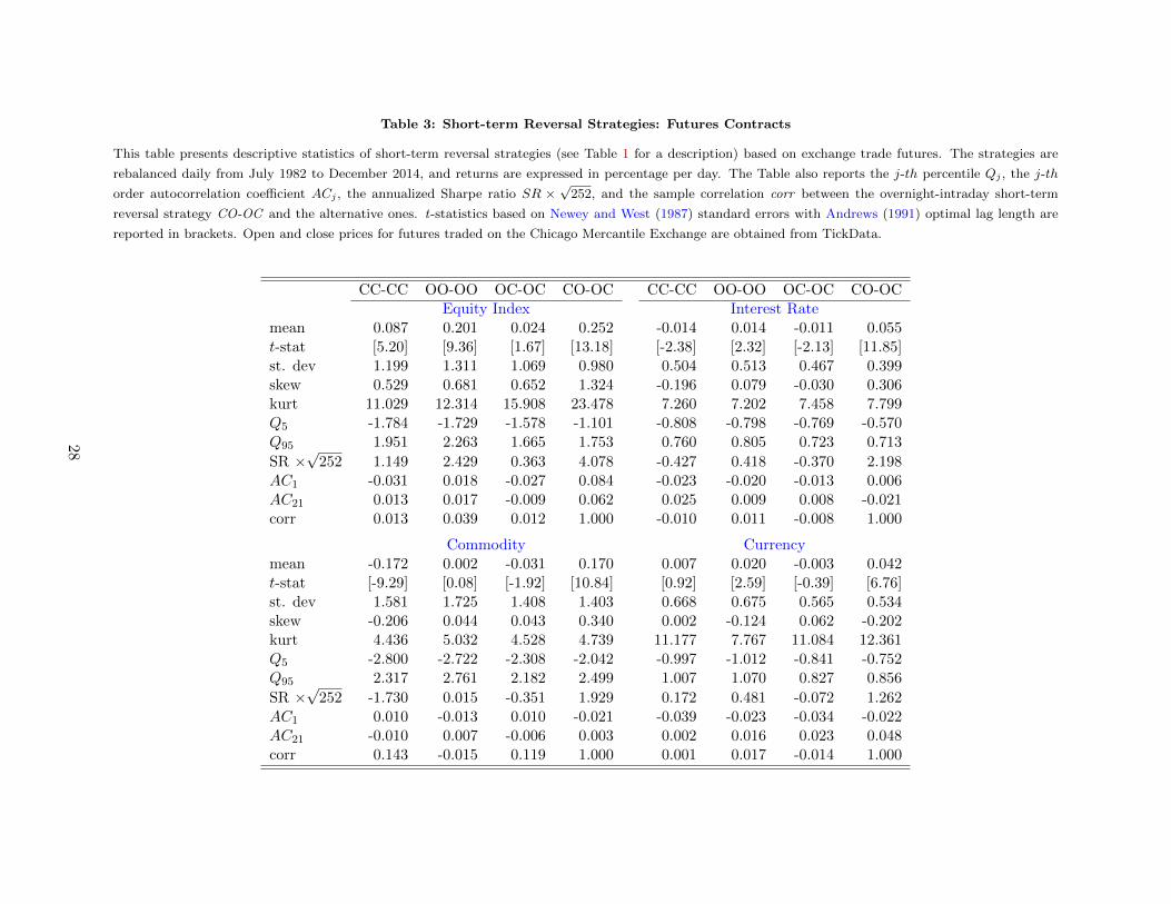
Table 3: Short-term Reversal Strategies: Futures Contracts

This table presents descriptive statistics of short-term reversal strategies (see Table 1 for a description) based on exchange trade futures. The strategies are

rebalanced daily from July 1982 to December 2014, and returns are expressed in percentage per day. The Table also reports the j-th percentile Qj , the j-th

order autocorrelation coefficient ACj , the annualized Sharpe ratio SR ×√

252, and the sample correlation corr between the overnight-intraday short-term

reversal strategy CO-OC and the alternative ones. t-statistics based on Newey and West (1987) standard errors with Andrews (1991) optimal lag length are

reported in brackets. Open and close prices for futures traded on the Chicago Mercantile Exchange are obtained from TickData.

CC-CC OO-OO OC-OC CO-OC CC-CC OO-OO OC-OC CO-OCEquity Index Interest Rate

mean 0.087 0.201 0.024 0.252 -0.014 0.014 -0.011 0.055t-stat [5.20] [9.36] [1.67] [13.18] [-2.38] [2.32] [-2.13] [11.85]st. dev 1.199 1.311 1.069 0.980 0.504 0.513 0.467 0.399skew 0.529 0.681 0.652 1.324 -0.196 0.079 -0.030 0.306kurt 11.029 12.314 15.908 23.478 7.260 7.202 7.458 7.799Q5 -1.784 -1.729 -1.578 -1.101 -0.808 -0.798 -0.769 -0.570Q95 1.951 2.263 1.665 1.753 0.760 0.805 0.723 0.713

SR ×√

252 1.149 2.429 0.363 4.078 -0.427 0.418 -0.370 2.198AC1 -0.031 0.018 -0.027 0.084 -0.023 -0.020 -0.013 0.006AC21 0.013 0.017 -0.009 0.062 0.025 0.009 0.008 -0.021corr 0.013 0.039 0.012 1.000 -0.010 0.011 -0.008 1.000

Commodity Currencymean -0.172 0.002 -0.031 0.170 0.007 0.020 -0.003 0.042t-stat [-9.29] [0.08] [-1.92] [10.84] [0.92] [2.59] [-0.39] [6.76]st. dev 1.581 1.725 1.408 1.403 0.668 0.675 0.565 0.534skew -0.206 0.044 0.043 0.340 0.002 -0.124 0.062 -0.202kurt 4.436 5.032 4.528 4.739 11.177 7.767 11.084 12.361Q5 -2.800 -2.722 -2.308 -2.042 -0.997 -1.012 -0.841 -0.752Q95 2.317 2.761 2.182 2.499 1.007 1.070 0.827 0.856

SR ×√

252 -1.730 0.015 -0.351 1.929 0.172 0.481 -0.072 1.262AC1 0.010 -0.013 0.010 -0.021 -0.039 -0.023 -0.034 -0.022AC21 -0.010 0.007 -0.006 0.003 0.002 0.016 0.023 0.048corr 0.143 -0.015 0.119 1.000 0.001 0.017 -0.014 1.000

28

Table 4: Short-term Reversal Strategies: Sub-periods

This table presents descriptive statistics of short-term reversal strategies (see Table 1 for a description) for two

different sub-periods. Panel A reports daily-rebalanced strategies based on international stock markets for the

periods January 1993 through December 2006, and January 2007 through December 2014. Panel B refers to

daily-rebalanced strategies that use exchange traded futures for the periods July 1982 through December 2006,

and January 2007 through December 2014. The excess returns are expressed in percentage per day. The Table

also reports the annualized Sharpe ratio SR ×√

252, and the sample correlation corr between the overnight-

intraday short-term reversal strategy CO-OC and the alternative ones. t-statistics based on Newey and West

(1987) standard errors with Andrews (1991) optimal lag length are reported in brackets. Open and close stock

prices are collected from the CRSP database for the US and Datastream for the other countries. Open and close

prices for futures traded on the Chicago Mercantile Exchange are obtained from TickData.

Panel A: International StocksCC-CC OO-OO OC-OC CO-OC CC-CC OO-OO OC-OC CO-OC

1993-2006 2007-2014United States

mean 0.434 0.778 -0.256 2.034 0.146 0.358 -0.023 1.047t-stat [17.09] [29.38] [-19.09] [57.73] [6.53] [13.66] [-1.40] [25.85]

SR ×√

252 7.342 12.146 -5.718 33.376 2.421 6.303 -0.683 16.070corr 0.293 0.135 0.072 1.000 0.071 0.190 0.049 1.000

Europe (France and Germany)mean 0.188 0.521 -0.229 0.941 0.307 1.240 -0.164 1.151t-stat [11.54] [18.66] [-17.15] [33.21] [14.63] [27.57] [-8.68] [33.86]

SR ×√

252 3.365 6.760 -5.458 16.161 5.096 10.179 -3.422 18.090corr 0.151 0.139 0.079 1.000 0.032 -0.008 0.038 1.000

Japanmean 0.383 0.727 0.060 0.856 0.037 0.676 0.000 0.535t-stat [21.23] [27.63] [6.01] [38.96] [1.88] [18.15] [-0.02] [21.39]

SR ×√

252 7.087 11.286 1.311 19.819 0.481 8.426 -0.258 11.463corr 0.243 0.223 0.141 1.000 0.090 0.054 0.235 1.000

United Kingdommean -0.504 0.373 -0.818 2.111 0.222 0.576 -0.391 1.629t-stat [-19.30] [8.25] [-26.69] [31.23] [8.04] [17.57] [-15.36] [39.14]

SR ×√

252 -6.963 3.542 -11.513 16.757 3.023 7.605 -6.512 21.708corr -0.015 0.146 -0.283 1.000 -0.023 0.109 -0.131 1.000

Panel B: Futures1982-2006 2007-2014

Equity Indexmean 0.070 0.155 0.020 0.166 0.108 0.260 0.030 0.364t-stat [2.91] [5.98] [0.51] [7.39] [5.02] [7.63] [1.46] [12.32]

SR ×√

252 0.809 1.708 0.274 2.508 1.906 3.718 0.524 6.683corr -0.017 -0.039 -0.019 1.000 0.081 0.190 0.075 1.000

Interest Ratemean -0.020 0.014 -0.015 0.053 0.004 0.012 -0.001 0.061t-stat [-3.31] [2.24] [-2.91] [10.40] [0.28] [0.91] [-0.07] [5.77]

SR ×√

252 -0.718 0.477 -0.591 2.306 0.090 0.309 -0.028 2.028corr 0.059 -0.005 0.110 1.000 -0.109 0.036 -0.160 1.000

Commoditymean -0.163 0.037 0.031 0.133 -0.203 -0.110 -0.229 0.290t-stat [-7.56] [1.68] [1.80] [7.74] [-5.55] [-2.91] [-6.42] [8.28]

SR ×√

252 -1.629 0.334 0.368 1.548 -2.053 -1.045 -2.341 3.027corr 0.167 -0.021 0.168 1.000 0.079 0.010 0.011 1.000

Currencymean -0.001 0.024 -0.008 0.038 0.025 0.013 0.009 0.052t-stat [-0.09] [2.56] [-1.41] [5.16] [1.66] [0.86] [0.58] [4.12]

SR ×√

252 -0.021 0.588 -0.257 1.258 0.536 0.280 0.190 1.301corr 0.046 -0.003 0.019 1.000 -0.062 0.045 -0.049 1.000

29

Table 5: Short-term Reversal Strategies: Sub-samples

This table presents descriptive statistics of short-term reversal strategies (see Table 1 for a description) for different sub-samples of US stocks. The strategies

are rebalanced daily from January 1993 to December 2014, and returns are expressed in percentage per day. The Table also reports the j-th percentile Qj , the

j-th order autocorrelation coefficient ACj , the annualized Sharpe ratio SR×√

252, and the sample correlation corr between the overnight-intraday short-term

reversal strategy CO-OC and the alternative ones. t-statistics based on Newey and West (1987) standard errors with Andrews (1991) optimal lag length are

reported in brackets. Open and close prices are collected from the CRSP database for the United States, and Datastream for all other countries.

CC-CC OO-OO OC-OC CO-OC CC-CC OO-OO OC-OC CO-OCSmall Stocks Large Stocks

mean 0.628 0.970 -0.223 2.328 0.077 0.264 -0.091 0.781t-stat [20.20] [31.36] [-16.65] [55.17] [6.59] [17.67] [-7.92] [32.41]st. dev 1.049 1.034 0.773 1.230 0.938 1.035 0.824 1.058skew 0.983 1.154 1.510 0.201 0.729 1.864 1.065 1.659kurt 7.552 15.731 21.611 6.060 15.021 27.354 26.045 18.266Q5 -0.822 -0.437 -1.332 0.408 -1.252 -1.027 -1.192 -0.654Q95 2.369 2.612 0.832 4.090 1.382 1.641 1.006 2.283

SR ×√

252 9.341 14.721 -4.788 29.909 1.130 3.885 -1.962 11.550AC1 0.392 0.384 0.075 0.524 0.002 -0.002 0.030 0.158AC21 0.356 0.351 0.086 0.465 0.038 0.024 0.040 0.118corr 0.368 0.397 -0.107 1.000 0.086 -0.010 0.123 1.000

S&P500 Stocks S&P100 Stocksmean 0.077 0.215 -0.002 0.429 0.046 0.190 0.000 0.347t-stat [5.97] [13.85] [-0.20] [23.07] [3.06] [11.69] [0.01] [19.18]st. dev 1.014 1.089 0.868 1.116 1.205 1.309 1.025 1.313skew 0.756 1.618 1.211 1.050 0.668 1.257 0.939 0.511kurt 14.408 17.932 19.276 11.473 16.215 20.983 18.616 14.782Q5 -1.351 -1.236 -1.183 -1.189 -1.703 -1.601 -1.452 -1.371Q95 1.579 1.831 1.223 2.147 1.724 1.997 1.399 2.249

SR ×√

252 1.036 2.977 -0.237 5.957 0.469 2.181 -0.164 4.073AC1 -0.021 -0.010 0.015 0.041 -0.062 -0.042 -0.013 -0.028AC21 0.012 -0.001 0.023 0.005 0.017 -0.005 0.022 -0.002corr 0.060 -0.039 0.151 1.000 0.045 -0.034 0.125 1.000

30

Table 6: Short-term Reversal Strategies: Bid and Ask Quotes

This table presents descriptive statistics of the overnight-intraday reversal strategy (see Table 1 for a description)

based on S&P500 stocks. We use bid quotes in Panel A, ask quotes in Panel B, and mid quotes in Panel C. The

strategies are rebalanced daily from January 2011 to December 2014, and returns are expressed in percentage per

day. The Table also reports the j-th percentile Qj , the j-th order autocorrelation coefficient ACj , the annualized

Sharpe ratio SR ×√

252, and the sample correlation corr between the overnight-intraday short-term reversal

strategy CO-OC and the alternative ones. t-statistics based on Newey and West (1987) standard errors with

Andrews (1991) optimal lag length are reported in brackets. Bid and ask quotes are obtained from the TAQ

database.

CC-CC OO-OO OC-OC CO-OCPanel A: Bid Quote

mean 0.031 0.398 -0.222 1.262t-stat [1.54] [13.37] [-11.35] [20.55]st. dev 0.644 0.679 0.487 1.041skew 1.490 0.271 0.048 1.173kurt 24.557 11.246 5.579 15.365Q5 -0.895 -0.536 -0.990 -0.198Q95 0.967 1.477 0.524 2.999

SR ×√

252 0.508 9.064 -7.575 19.091AC1 0.071 0.172 0.143 0.360AC21 -0.032 0.014 0.028 0.232corr 0.005 0.218 -0.160 1.000

Panel B: Ask Quotemean 0.029 0.348 -0.197 1.152t-stat [1.45] [12.95] [-11.01] [21.89]st. dev 0.615 0.656 0.469 0.951skew 0.343 0.327 0.096 1.707kurt 10.456 11.289 5.659 23.732Q5 -0.891 -0.573 -0.931 -0.156Q95 0.959 1.373 0.549 2.691

SR ×√

252 0.464 8.155 -7.034 19.046AC1 0.055 0.138 0.138 0.316AC21 -0.036 -0.004 -0.011 0.173corr -0.010 0.179 -0.109 1.000

Panel C: Mid Quotemean 0.027 0.127 -0.065 0.432t-stat [1.37] [5.91] [-4.25] [14.83]st. dev 0.607 0.607 0.462 0.766skew 0.062 -0.297 0.002 0.291kurt 8.338 8.448 6.179 10.001Q5 -0.894 -0.781 -0.773 -0.674Q95 0.958 1.066 0.655 1.641

SR ×√

252 0.427 3.036 -2.604 8.738AC1 0.059 0.089 0.066 0.091AC21 -0.038 -0.072 -0.037 0.004corr 0.032 0.065 0.062 1.000

31

Table 7: Short-term Reversal Strategies: Transaction data

This table presents descriptive statistics of the overnight-intraday reversal strategy (see Table 1 for a description)

based transaction prices for the S&P 500 stocks. In Panel A the formation windows uses returns observed at 9:30am

whereas the trading period starts between 9.30 am and 9.45 am. In Panel B (Panel C ) the formation windows

uses returns observed at 9:29 am (9.25 am). The strategies are rebalanced daily from January 2011 to December

2014, and returns are expressed in percentage per day. The Table also reports the j-th percentile Qj , the j-th order

autocorrelation coefficient ACj , the annualized Sharpe ratio SR×√

252, and the sample correlation corr between

the overnight-intraday short-term reversal strategy CO-OC and the alternative ones. t-statistics based on Newey

and West (1987) standard errors with Andrews (1991) optimal lag length are reported in brackets. Transaction

prices are from the TAQ database.

Panel A: Formation period ends at 9.30 am (opening)Trading period starts at 9.30 am 9.31 am 9.32 am 9.33 am 9.34 am 9.35 am 9.40 am 9.45 am

mean 0.359 0.112 0.108 0.105 0.088 0.089 0.050 0.042t-stat [10.98] [3.81] [3.74] [3.74] [3.31] [3.38] [2.19] [1.99]st. dev 0.964 0.885 0.868 0.840 0.804 0.809 0.716 0.667skew 0.416 0.590 0.579 0.793 0.791 0.733 0.345 0.560kurt 8.120 9.438 10.634 9.953 9.070 9.719 7.586 6.223Q5 -1.035 -1.159 -1.155 -1.129 -1.187 -1.088 -0.997 -0.998Q95 1.926 1.534 1.437 1.417 1.379 1.328 1.120 1.117

SR ×√

252 5.746 1.818 1.778 1.787 1.524 1.548 0.872 0.734AC1 0.022 -0.013 -0.006 0.000 -0.001 -0.008 -0.022 -0.026AC21 -0.035 -0.008 -0.010 -0.012 -0.009 -0.010 -0.035 -0.038

Panel B: Formation period ends at 9.29 am (pre-opening)mean 0.340 0.109 0.106 0.104 0.087 0.088 0.049 0.041t-stat [10.39] [3.78] [3.69] [3.72] [3.30] [3.37] [2.19] [2.03]st. dev 0.960 0.880 0.867 0.838 0.801 0.806 0.714 0.664skew 0.376 0.544 0.564 0.765 0.765 0.696 0.278 0.496kurt 8.074 9.357 10.682 9.813 8.967 9.637 7.449 5.998Q5 -1.047 -1.170 -1.141 -1.120 -1.133 -1.076 -1.011 -1.017Q95 1.922 1.542 1.469 1.440 1.372 1.327 1.109 1.123

SR ×√

252 5.441 1.781 1.742 1.762 1.503 1.526 0.856 0.735AC1 0.018 -0.023 -0.014 -0.010 -0.011 -0.020 -0.032 -0.041AC21 -0.036 -0.009 -0.014 -0.015 -0.013 -0.012 -0.039 -0.040

Panel C: Formation period ends at 9.25 am (pre-opening)mean 0.310 0.112 0.125 0.126 0.108 0.108 0.039 0.029t-stat [8.09] [3.31] [3.72] [3.92] [3.55] [3.62] [1.56] [1.27]st. dev 1.127 1.041 1.027 0.986 0.943 0.946 0.752 0.684skew 0.512 0.695 0.686 0.872 0.828 0.647 -0.976 -0.555kurt 9.841 11.227 13.363 10.946 10.260 10.482 15.608 11.983Q5 -1.333 -1.367 -1.266 -1.270 -1.268 -1.265 -0.991 -0.922Q95 2.053 1.692 1.676 1.636 1.528 1.519 1.156 1.078

SR ×√

252 4.217 1.549 1.766 1.854 1.638 1.626 0.592 0.415AC1 0.004 -0.034 -0.030 -0.035 -0.030 -0.049 0.004 0.010AC21 -0.017 0.007 -0.002 0.001 0.000 -0.002 -0.055 -0.065

32

Table 8: Short-term Reversal Strategies: Weekly international stocks

This table presents descriptive statistics of weekly reversal strategy (similar to those described in Table 1) based on international stock markets. The strategies

are rebalanced weekly from January 1993 to December 2014, and returns are expressed in percentage per week. The Table also reports the j-th percentile

Qj , the j-th order autocorrelation coefficient ACj , the annualized Sharpe ratio SR ×√

52, and the sample correlation corr between the overnight-intraday

short-term reversal strategy CO-OC and the alternative ones. t-statistics based on Newey and West (1987) standard errors with Andrews (1991) optimal lag

length are reported in brackets. Open and close prices are collected from the CRSP database for the United States, and Datastream for all other countries.

CC-CC OO-OO OC-OC CO-OC CC-CC OO-OO OC-OC CO-OCUnited States Europe (France and Germany)

mean 0.699 0.878 0.445 1.870 0.666 1.029 0.289 1.363t-stat [12.81] [16.42] [10.49] [23.44] [14.23] [17.42] [7.16] [20.61]st. dev 1.718 1.623 1.661 1.633 1.607 1.910 1.573 1.640skew 1.303 0.996 1.154 0.541 0.658 0.691 0.219 1.039kurt 11.834 9.973 14.111 9.524 7.533 6.183 7.062 7.592Q5 -1.512 -1.305 -1.802 -0.540 -1.667 -1.849 -2.147 -0.864Q95 3.313 3.357 3.040 3.924 3.221 4.140 2.713 4.179

SR ×√

52 2.711 3.665 1.700 8.020 2.749 3.685 1.079 5.757AC1 -0.051 -0.046 -0.136 0.269 -0.042 0.007 -0.051 0.131AC4 0.073 0.080 0.042 0.164 0.070 0.090 0.065 0.073corr 0.001 0.186 -0.032 1.000 0.008 0.071 -0.002 1.000

Japan United Kingdommean 0.641 1.103 0.409 1.049 0.410 0.680 0.240 1.409t-stat [10.14] [16.54] [8.62] [17.56] [7.62] [10.60] [4.51] [16.67]st. dev 1.691 1.888 1.586 1.399 1.823 2.005 1.775 2.185skew 0.943 1.047 0.844 1.203 0.234 0.696 0.315 1.691kurt 7.599 8.174 7.931 9.402 11.184 10.715 9.267 12.282Q5 -1.808 -1.606 -1.960 -0.970 -2.047 -1.995 -2.434 -1.462Q95 3.411 4.032 2.766 3.154 3.224 3.741 2.866 4.724

SR ×√

52 2.506 4.010 1.620 5.132 1.410 2.254 0.758 4.475AC1 0.081 0.049 -0.044 0.152 -0.063 -0.011 -0.046 0.083AC4 0.083 0.048 0.038 0.134 -0.014 0.025 0.001 0.043corr 0.194 0.153 0.183 1.000 0.066 0.073 0.005 1.000

33

Table 9: Short-term Reversal Strategies: Weekly futures

This table presents descriptive statistics of weekly reversal strategy (similar to those described in Table 1) based on exchange traded futures. The strategies

are rebalanced weekly from July 1982 to December 2014, and returns are expressed in percentage per week. The Table also reports the j-th percentile Qj , the

j-th order autocorrelation coefficient ACj , the annualized Sharpe ratio SR ×√

52, and the sample correlation corr between the overnight-intraday short-term

reversal strategy CO-OC and the alternative ones. t-statistics based on Newey and West (1987) standard errors with Andrews (1991) optimal lag length are

reported in brackets. Open and close prices for futures traded on the Chicago Mercantile Exchange are obtained from TickData.

CC-CC OO-OO OC-OC CO-OC CC-CC OO-OO OC-OC CO-OCEquity Index Interest Rate

mean 0.089 0.267 0.057 0.379 0.055 0.073 0.038 0.128t-stat [1.09] [3.45] [0.66] [4.18] [1.94] [2.46] [1.30] [4.46]st. dev 2.563 2.285 2.643 2.325 1.107 1.165 1.135 1.036skew 0.836 1.069 0.714 0.684 0.515 0.920 0.638 0.879kurt 12.353 9.080 10.408 7.978 6.127 11.694 8.418 12.151Q5 -3.750 -3.353 -3.646 -3.120 -1.612 -1.573 -1.576 -1.422Q95 4.134 4.410 3.987 3.894 1.853 1.951 1.887 1.802

SR ×√

52 0.251 0.842 0.157 1.176 0.358 0.454 0.244 0.894AC1 -0.169 -0.010 -0.159 0.062 0.007 -0.020 0.002 -0.042AC4 -0.016 0.109 0.024 0.041 0.009 0.004 0.015 -0.060corr -0.081 0.039 -0.040 1.000 0.020 -0.048 0.054 1.000

Commodity Currencymean -0.077 0.072 -0.012 0.173 0.071 0.084 0.048 0.169t-stat [-0.86] [0.76] [-0.14] [1.94] [2.00] [2.30] [1.38] [4.45]st. dev 3.777 3.841 3.746 3.714 1.415 1.372 1.362 1.354skew -0.187 -0.236 -0.242 -0.049 -0.380 0.176 -0.278 0.408kurt 5.640 5.302 5.682 5.109 14.394 8.625 12.907 5.065Q5 -6.270 -6.024 -6.013 -5.875 -1.904 -1.950 -1.933 -1.996Q95 5.821 6.223 5.796 5.905 2.364 2.237 2.318 2.356

SR ×√

52 -0.147 0.135 -0.024 0.337 0.360 0.442 0.256 0.897AC1 0.052 0.084 0.047 0.031 0.028 0.054 0.048 0.009AC4 0.026 0.026 0.028 -0.026 0.008 0.023 0.011 0.049corr 0.037 0.034 0.025 1.000 0.043 0.061 0.042 1.000

34

Table 10: Short-term Reversal Strategies: FOMC announcement

This table presents descriptive statistics of short-term reversal strategies (see Table 1 for a description) for FOMC

and non-FOMC announcement days. Panel A reports daily-rebalanced strategies based on international stock

markets for the periods January 1993 through December 2006, and January 2007 through December 2014. Panel B

refers to daily-rebalanced strategies that use exchange traded futures for the periods July 1982 through December

2006, and January 2007 through December 2014. The excess returns are expressed in percentage per day. The

Table also reports the annualized Sharpe ratio SR×√

252, and the sample correlation corr between the overnight-

intraday short-term reversal strategy CO-OC and the alternative ones. t-statistics based on Newey and West

(1987) standard errors with Andrews (1991) optimal lag length are reported in brackets. Open and close stock

prices are collected from the CRSP database for the US and Datastream for the other countries. Open and close

prices for futures traded on the Chicago Mercantile Exchange are obtained from TickData.

Panel A: International StocksFOMC Announcement non-FOMC Announcement

CC-CC OO-OO OC-OC CO-OC CC-CC OO-OO OC-OC CO-OCUnited States

mean 0.396 0.703 -0.131 1.601 0.323 0.617 -0.175 1.683t-stat [7.61] [12.63] [-4.04] [18.15] [15.67] [26.66] [-14.44] [45.37]

SR ×√

252 6.955 12.874 -3.166 24.576 5.378 9.711 -3.858 24.132corr 0.168 0.398 -0.152 1.000 0.262 0.211 0.006 1.000

Europe (France and Germany)mean 0.292 0.863 -0.125 1.018 0.225 0.774 -0.214 1.017t-stat [7.69] [10.34] [-3.64] [15.62] [16.07] [25.42] [-18.08] [42.40]

SR ×√

252 5.135 9.461 -2.853 14.803 3.909 7.820 -4.820 17.046corr 0.075 0.053 -0.001 1.000 0.112 0.090 0.074 1.000

Japanmean 0.264 0.745 0.021 0.747 0.257 0.705 0.040 0.739t-stat [5.76] [11.73] [0.65] [16.00] [15.52] [30.58] [4.34] [37.97]

SR ×√

252 4.571 10.563 0.243 16.243 4.543 9.989 0.744 16.250corr 0.095 0.216 0.262 1.000 0.231 0.144 0.177 1.000

United Kingdommean -0.274 0.440 -0.700 2.003 -0.236 0.447 -0.659 1.928t-stat [-3.25] [4.49] [-8.67] [13.65] [-9.11] [13.45] [-27.86] [40.09]

SR ×√

252 -3.066 4.216 -8.731 16.188 -3.343 4.731 -9.805 17.565corr -0.080 0.186 -0.379 1.000 -0.050 0.121 -0.248 1.000

Panel B: FuturesEquity Index

mean 0.101 0.229 0.060 0.213 0.085 0.198 0.021 0.256t-stat [1.49] [2.73] [1.14] [3.64] [5.07] [9.12] [0.94] [13.10]

SR ×√

252 1.087 2.578 0.750 3.055 0.999 2.270 0.149 4.003corr -0.054 0.120 -0.029 1.000 0.021 0.030 0.017 1.000

Interest Ratemean 0.021 0.080 0.024 0.053 -0.016 0.008 -0.014 0.055t-stat [0.72] [3.87] [1.06] [2.66] [-2.79] [1.41] [-2.66] [11.25]

SR ×√

252 0.285 1.961 0.403 1.607 -0.858 -0.071 -0.835 1.788corr -0.024 0.054 -0.071 1.000 -0.009 0.007 -0.002 1.000

Commoditymean -0.170 -0.057 -0.051 0.165 -0.172 0.006 -0.030 0.171t-stat [-2.32] [-0.81] [-0.77] [2.88] [-9.00] [0.28] [-1.81] [10.54]

SR ×√

252 -1.781 -0.607 -0.659 1.753 -1.841 -0.045 -0.457 1.812corr 0.105 -0.041 0.099 1.000 0.146 -0.013 0.120 1.000

Currencymean 0.084 0.076 0.083 0.064 0.001 0.016 -0.010 0.041t-stat [2.66] [2.91] [2.99] [2.95] [0.08] [1.90] [-1.64] [6.13]

SR ×√

252 1.654 1.606 1.917 1.630 -0.239 0.118 -0.581 0.887corr -0.032 0.039 0.025 1.000 0.004 0.015 -0.018 1.000

35

Table 11: Predictability: the role of VIX

This table reports the results of the regression: ∆returnCO−OCt = α + β1∆V IXt−1 + β2V IX

nightt−1 + ε. We use

the following volatility index for each equity market: US: CBOE S&P 500 implied volatility index (VIX); Europe:

EURO STOXX 50 volatility (VSTOXX); Japan: Nikkei stock average volatility index (VNKY); UK: FTSE 100

implied volatility index (IVI). ∆V IX is the change of VIX close quote. V IXnight is the difference between open

quote and previous close quote. For futures, VIX is proxied by the cross-section return dispersion. t-statistics based

on Newey and West (1987) standard errors with Andrews (1991) optimal lag length are reported in brackets.

Dependent Variable: ∆CO −OCPanel A: International Stocks

United States Europeintercept 0.000 -0.000 0.000 0.000

[0.00] [-1.78] [0.04] [-0.15]∆V IX 0.000 0.000 0.000 0.000

[1.38] [1.76] [1.46] [1.55]V IXnight 0.001 0.001

[3.04] [3.36]Adj R2 0.001 0.013 0.001 0.007

Japan United Kingdomintercept 0.000 0.000 0.000 0.000

[0.02] [0.55] [-0.04] [-0.03]∆V IX 0.000 0.000 0.000 0.000

[-0.20] [-0.16] [1.92] [2.00]V IXnight 0.001 0.000

[1.65] [3.63]Adj R2 -0.000 0.001 0.002 0.008

Panel B: Futures

Equity Index Interest Rateintercept 0.000 0.000 0.000 0.000

[0.16] [0.15] [-0.09] [-0.13]∆V IX 0.226 0.255 0.149 0.151

[8.01] [9.48] [7.31] [7.59]V IXnight 0.283 0.269

[6.83] [4.85]Adj R2 0.048 0.086 0.021 0.034

Commodity Currencyintercept 0.000 0.000 0.000 0.000

[-0.16] [-0.17] [0.03] [0.03]∆V IX 0.189 0.195 0.201 0.206

[13.44] [14.17] [8.76] [9.36]V IXnight 0.217 0.045

[9.57] [1.58]Adj R2 0.038 0.059 0.062 0.063

36

Figure 1: Autocorrelation Structure: International Stocks

Lagged days

0 1 2 3 4 5 6 7 8 9 10 11 12 13 14 15 16 17 18 19 20

T-s

tatis

tics

-60

-40

-20

-22

20United States

Intraday returnOvernight return

Lagged days

0 1 2 3 4 5 6 7 8 9 10 11 12 13 14 15 16 17 18 19 20

T-s

tatis

tics

-60

-40

-20

-22

20Europe (France & Germany)

Intraday returnOvernight return

Lagged days

0 1 2 3 4 5 6 7 8 9 10 11 12 13 14 15 16 17 18 19 20

T-s

tatis

tics

-60

-40

-20

-22

20Japan

Intraday returnOvernight return

Lagged days

0 1 2 3 4 5 6 7 8 9 10 11 12 13 14 15 16 17 18 19 20

T-s

tatis

tics

-60

-40

-20

-22

20United Kingdom

Intraday returnOvernight return

This figure plots the average Fama-MacBeth coefficients of the autocorrelation test: roci,t = β0 +∑20

1 βk,t ∗ roci,t−k +∑20

1 γk,t ∗ rcoi,t−k + εi,t.The t-statistic for the first lag (rco) is computed using standard errors that are clustered by time and asset, in order to account for thetime-series dependence of the estimates in the first step. The sample is from January 1993 to December 2014.

37

Figure 2: Autocorrelation Structure: Futures

Lagged days

0 1 2 3 4 5 6 7 8 9 10 11 12 13 14 15 16 17 18 19 20

T-s

tatis

tics

-10

-5

-2

2

5Equity Index

Intraday returnOvernight return

Lagged days

0 1 2 3 4 5 6 7 8 9 10 11 12 13 14 15 16 17 18 19 20

T-s

tatis

tics

-10

-5

-2

2

5Fixed Income

Intraday returnOvernight return

Lagged days

0 1 2 3 4 5 6 7 8 9 10 11 12 13 14 15 16 17 18 19 20

T-s

tatis

tics

-10

-5

-2

2

5Commodity

Intraday returnOvernight return

Lagged days

0 1 2 3 4 5 6 7 8 9 10 11 12 13 14 15 16 17 18 19 20

T-s

tatis

tics

-10

-5

-2

2

5Currency

Intraday returnOvernight return

This figure plots the pooled OLS coefficients of the autocorrelation test: roci,t = β0 +∑20

1 βk,t ∗ roci,t−k +∑20

1 γk,t ∗ rcoi,t−k + εi,t. Thet-statistic are computed using standard errors that are clustered by time and asset, in order to account for the time-series dependenceof the estimates. The sample is from July 1982 to December 2014.

38

Figure 3: Intraday Dynamics of VIX

9:30 10:30 11:30 12:30 13:30 14:30 15:30 16:0020.1

20.15

20.2

20.25

20.3

20.35

20.4

20.45

20.5

This figure plots average intraday minute levels of VIX index from January 1993 to December2013.

39

Figure 4: Autocorrelation Structure: Simulation

Lagged days0 1 2 3 4 5 6 7 8 9 10 11 12 13 14 15 16 17 18 19 20

T-s

tatis

tics

-8

-7

-6

-5

-4

-3

-2

-1

0

Overnight ReturnIntraday Return

This figure plots the average coefficients of the simulated autocorrelation test based on the modelin Hong and Wang (2000). The regression formula is: roct = β0+

∑201 βk ∗roct−k+

∑201 γk ∗rcot−k+εt.

The model parameters are set at the following values: The lengths of open and close periods areT = 0.4 and N = 0.6, γ = 1000, r = 0.001, σD = σG = 0.08, σq = 0.5, σy = 0.25, σ1 = σ2 = 7,κDq = 0.65, κ12 = 0.

40

Figure 5: Autocorrelation Structure: the role of liquidity shock

Lagged days

0 1 2 3 4 5 6 7 8 9 10 11 12 13 14 15 16 17 18 19 20

T-s

tatis

tics

-10

-5

0

5volatility=1

Overnight ReturnIntraday Return

Lagged days

0 1 2 3 4 5 6 7 8 9 10 11 12 13 14 15 16 17 18 19 20

T-s

tatis

tics

-10

-5

0

5K

Dq=0.1

Overnight ReturnIntraday Return

Lagged days

0 1 2 3 4 5 6 7 8 9 10 11 12 13 14 15 16 17 18 19 20

T-s

tatis

tics

-10

-5

0

5volatility=30

Overnight ReturnIntraday Return

Lagged days

0 1 2 3 4 5 6 7 8 9 10 11 12 13 14 15 16 17 18 19 20

T-s

tatis

tics

-10

-5

0

5K

Dq=0.9

Overnight ReturnIntraday Return

This figure plots the average coefficients of the simulated autocorrelation test based on the model in Hong and Wang (2000). Theregression formula is: roct = β0 +

∑201 βk ∗ roct−k +

∑201 γk ∗ rcot−k + εt. The model parameters are set at the following values: The lengths

of open and close periods are T = 0.4 and N = 0.6, γ = 1000, r = 0.001, σD = σG = 0.08, σq = 0.5, σy = 0.25,κ12 = 0. We choosedifferent values for the volatility σ1 and σ2 and the stock’s exposure to the real investment opportunity κDq,

41

Figure 6: Pastor-Stambaugh Liquidity Factor

99 00 01 02 03 04 05 06 07 08 09 10 11 12 13 14-0.4

-0.2

0

0.2

0.4

0.6

0.8

1

1.2

1.4

1.6

PSIntradayOvernight

This figure reports the cumulative return of the traded Pastor-Stambaugh liquidity factor. Thetraded factor is the value-weighted return on the 10-1 portfolio from a sort on historical liquiditybetas.The blue curve shows the return of Pastor-Stambaugh factor. The red circle line depictsthe return of liquidity factor based on the measure with intraday return: re,oci,d+1,t = θi,t+φi,tr

oci,d,t+

γi,tsign(re,oci,d,t)× υi,d,t + εoci,d+1,t. The black diamond depicts the return of liquidity factor based on

the measure with overnight return: re,coi,d+1,t = θi,t + φi,trcoi,d,t + γi,tsign(re,coi,d,t)× υi,d,t + εcoi,d+1,t.

42

Internet Appendix to

“Market Closure and Short-Term Reversal”

(not for publication)

Abstract

This appendix presents supplementary results not included in the main body of the paper.

IA.A Amodel of periodic market closure: Hong andWang (2000)

Basic Setting

The economy is defined on a continuous time-horizon with a single commodity, which is also

used as a numeraire.

• The underlying uncertainty is characterized by an n-dimensional standard Wiener process,

wt.

• Two types of investors, with proportion ω and 1− ω, denoted by i=1,2.

• Investment opportunities: public (risk-free money market and a risky stock), private

investment technologies only available to individual investors in each group. Payoffs as

following:

– Risk-free rate of return r.

– Each share of the stock pays a cumulative dividend Dt where

Dt =

∫ t

0(Gsds+ bDdws); (IA.A.1)

Gt = G0 +

∫ t

0(−aGGsds+ bGdws); (IA.A.2)

– Investor i’s private technology yields a cumulative excess return qi,t, where

qi,t =

∫ t

0(Yi,sds+ bqdws); (IA.A.3)

Yi,t = Yi,0 +

∫ t

0(−aY Yi,sds+ bidws); (IA.A.4)

Here, i=1,2, aG, aY are positive constant, bD,bG,bq,b1,b2 are constant matrices.

– The system Gt, Y1,t, Y2,t follow Gaussian Markov process, which determines the dis-

tribution of future payoffs on stock and private technologies. For convenience, let

Zt = [Gt, Y1,t, Y2,t]′.

Zt = Z0 +

∫ t

0−azZsds+ bZdws); (IA.A.5)

where Z0 = [G0;Y1,0;Y2,0], aZ = [[aG,0,0]; [0,aY,0]; [0,0,aY]], and bZ = [bG; b1; b2]

IA – 1

• The investors can continuously invest in private technologies and money market, while the

stock market is open periodically and the price is denoted as Pt.

• Periodic Stock Market: [tk, nk] denote the k-th trading period, and (nk, tk+1) is the

k-th non-trading period, where k=1,2...... Length of trading period T (nk − tk = T ) and

non-trading period N (tk+1 − nk=N) are constant. T = ∪k [tk ,nk ] is the set of times of

trading periods, and N = ∪k [nk , tk+1 ] is set of times the stock market is closed.

• Information: All investors observe realized dividends and prices. Class 1 investors observe

all state variables (Gt, Y1,t, Y2,t), but class 2 investors only observe (Y2,t). Additionally, a

set of public signal by Ut where

Ut = U0 +

∫ t

0aUZsds+ bUdws); (IA.A.6)

U0 is joint normal with G0, Y1,0, Y2,0, and aU,bU are constant matrices.

• Endowments, Policies, and Preferences: let ci,t (t ∈ [0,∞)) be his consumption, yi,t

(t ∈ [0,∞)) be the investment in private technology, and θi,t (t ∈ T ) the number of stock

shares he holds at time t, and they are adapted to information Ii,t. All investors have the

following expected utility:

E[−∫ ∞t

e−ρ(s−t)−γci,sds|Ii,t] (IA.A.7)

• Distributional Assumptions:

Assume

wt = [wD,t;wG,t;w1,t;w2,t;wq,t; wU,t]

and

bD = σD[1, 0, 0, 0, 0,0]; bG = σG[0, 1, 0, 0, 0,0]; bq = σq[κDq, 0, 0, 0,√

1− κ2Dq,0];

b1 = σ1[0, 0, κ−, κ+,0]; b2 = σ2[0, 0, κ+, κ−, 0,0]; bU = σU [0, 0, 0, 0, 0,0];

where κDq ∈ (−1, 1) and κ± = 12(√

1 + κ12 ±√

1− κ12)

• Additional Notation:

IA – 2

Define the expected value of future dividends discounted by risk-free rate under full infor-

mation,

Ft = Et[

∫ ∞t

e−r(s−t)dDs ] =1

r + aGGt (IA.A.8)

Also define

dQt = dPt + dDt − rPtdt (IA.A.9)

to be the instantaneous excess return when market is open and e = E[dQt]/dt, σ2Q =

E[(dQt)2]/dt its first two unconditional moments.

Rs,t = Pt − Ps +

∫ t

sDτdτ (IA.A.10)

where s, t ∈ T

Definition of Equilibrium

Investor i’s financial wealth consist of two parts: the balance in a money-market account W 0i,t

and the stock position θi,t. During the day, the stock market is open, investor can freely adjust

his stock position and money-market account to finance consumption and investment in private

technology, and the total financial wealth is: Wi,t = W 0i,t + θi,tPt. During the night, the budget

constraint is by W 0i,t, and the overnight stock position θi,nk

is an additional state variable.

Each investors’ optimization problem can now be expressed:

t ∈ Tk : Ji,t = sup{ci,yi,θi}

E[−∫ nk

te−ρ(s−t)−γci,tds+ J∗

i,n+k

|Ii,t] (IA.A.11)

s.t. dWi,t = (rWi,t − ci,t)dt+ θi,tdQt + yi,tdqi,t

t ∈ Nk : J∗i,t = sup{ci,yi}

E[−∫ tk+1

te−ρ(s−t)−γci,tds+ Ji,tk+1

|Ii,t] (IA.A.12)

s.t. dW 0i,t = (rW 0

i,t − ci,t)dt+ θi,nkdDt + yi,tdqi,t

where Ji,t, J∗i,t denote value function during day and night, and t−, t+ the time right before and

IA – 3

after t. At the open and close, the boundary conditions are:

Ji,nk= E[J∗

i,n+k

|Ii,nk] J∗

i,t−k+1

= E[Ji,tk+1|Ii,t−k+1

] (IA.A.13)

The stock market clears:

ωθ1,t + (1− ω)θ2,t = 1 ∀t ∈ T (IA.A.14)

Definition 1:

A periodic equilibrium is defined by the stock price function P (•; t) and the policy functions

ci(•; t), yi(•; t), θi(•; t), i = 1, 2, such that (a) the policies maximize expected utility, (b) the stock

market clears, (c) the price function and policy functions are periodic in t with periodicity T +N .

This paper restrict to the linear equilibrium in which price function is linear in the sufficient

statistics for Ii,t.

Conjecture of the Equilibrium

The conjectured price function is linear in the conditional expectations of both investors:

Pt = λ1E1,t[Zt] + λ2E2,t[Zt]− λ0 ∀t ∈ T (IA.A.15)

where λi = [λiG,−λi1,−λi2] (i = 1, 2), defined on T , is deterministic but time-dependent with

periodicity T + N . Define Gt = E2,t(Gt) and Y1,t = E2,t[Y1,t]. Then the price function is:

Pt = λ1GGt − λ11Y1,t − λ12Y2,t + λ2GGt − λ21Y1,t + λ22Y2,t − λ0 (IA.A.16)

Characterization of the Equilibrium To characterize the equilibrium, we take the price

function (16) as given and derive teach investor’s expectations and policies and conditions for

IA – 4

market clearing.

• Conditional Expectations

Investor i receives a vector of signals Si,t: S1,t = [Ut;Dt;Pt;Gt;Y1,t;Y2,t; q1,t] and S2,t =

[Ut;Dt;Pt;Y2,t; q2,t]. Thus, Ii ,t = {Si,t : 0 ≤ s ≤ t}. Since Zt and Si,t are jointly Gaussian,

the distribution of Zt conditional on {St} is Gaussian, fully characterized by its mean and

variance. Let Zi,t = Ei,t[Zt] and oi(t) = Ei,t[(Zt − Zi,t)(Zt − Zi,t)′].

Lemma 1:

∀t > s : Zi,t = e−aZ(t−s)Zi,s +

∫ t

se−aZ(t−τ)ki(dSi,τ − Ei,τ [dSi,τ ]) (IA.A.17)

∀t > s : oi(t) = oi(s) +

∫ t

sgi,odτ (IA.A.18)

where ki and gi,o are deterministic. oi evolves deterministically over time. The periodic

solution to the investors’ expectations requires that:

oi(tk+1) = oi(tk), k = 0, 1, 2.... (IA.A.19)

• Optimal Policies

Define Xt = [1, Y1,t, Y2,t, Gt − Gt, Y1,t − Y1,t]′ as a sub vector of the state variables and let

Xi,t = Ei,t[Xt] denotes the conditional expectation. The price function can be rewritten as

follows:

Pt = Ft − λXt = Fi,t − λiXi,t ∀t ∈ T (IA.A.20)

where λ = [λ0, λ1, λ2,1

r+aG− λG, 0], Fi,t = Ei,t(Ft), λ1 = λ and λ2 = [λ0, λ1, λ2, 0, 0].

∀t > s : Xi,t = Xi,0 +

∫ t

0{−ai,XXi,sds+ ki,X(dSi,s − Ei,s[dSi,s])} (IA.A.21)

and

∀t ∈ T : Qt =

∫ t

0{ai,QXi,tds+ ki,Q(dSi,s − Ei,s[dSi,s])} (IA.A.22)

Lemma 3

IA – 5

Given the price function (20) and the solution to investors’ expectation, investor i’s value

function has the form:

t ∈ Tk : Ji,t = −exp{−ρt− rγWi,t − 12X′i,tυiXi,t}

t ∈ Nk : J∗i,t = −exp{−ρt− rγW ∗i,t − 12X′∗i,tυiX

∗i,t}

(IA.A.23)

where W ∗i,t = W 0i,t + θi,nk

Fi,t, X∗i,t = [Xi,t; θi,nk], υi is a symmetric matrix, given by

∀s < t : υi(s) = υi(t) +

∫ s

tgi,vdτ (IA.A.24)

and

υi(tk) = υi(tk+1) (IA.A.25)

with gi,v being deterministic. The optimal policies are

t ∈ [tk, nk] :

θi,tyi,t

=

hi,θ

hi,y

Xi,t

ci,t = −1r lnγ + rWi,t + 1

2γX′i,tυiXi,t

(IA.A.26)

t ∈ (nk, tk+1) :

yi,t = [hi,y, hi]X∗i,t

ci,t = −1r lnγ + rW ∗i,t + 1

2γX′∗i,tυiX∗i,t

where hi,θ, hi,y and hi are functions of λi, oi, υi.

Given λ and resulting oi, Lemma 3 expresses investor i’s optimal policies as functions of υi,

which is in (24), a (vector-form) first-order ODE with boundary condition (25).

• Market Clearing

Stock market clearing condition requires:

ωλ1h1,θ + (1− ω)h2,θτ = [1,0,0,0,0] ∀t ∈ Tk (IA.A.27)

IA – 6

where τ = [[λ, 0, 0, 0, 0]; [0, λ1, 0,−λG, 0]; [0, 0, λ1, 0, 0]]. The periodic condition requires

λ(tk) = λ(tk+1) (IA.A.28)

Given hi,θ, equation (27) defines first-order ODE for λ and boundary condition is (28).

Computation of the Equilibrium

The periodic equilibrium now reduces to solving a system of first-order ODE’s for oi, υi and

λ, subject to periodicity conditions (19), (25) and (28).

In general, the actual values of oi, υi and λ can only be solved numerically. We need start

with the solution at ω = 1 and then obtain solutions for values of ω close to one. Iteratively, we

arrive at the solutions for desired valued of ω.

The Case of Symmetric Information

This case can be obtained from the general model by letting U0 = Z0, aU = [[1, 0, 0]; [0, 1, 0]; [0, 0, 1]]

and bU = 0. Gt, Y1,t, Y2,t then become public information.

The stock price under symmetric information is

Pt = Ft − (λ0 + λ1Y1,t + λ2Y2,t) ∀t ∈ T (IA.A.29)

It is given by the value of expected future dividends (Ft) minus a risk discount (λ0+∑

i λiYi,t).

The risk discount consists of two parts: (a) an unconditional part (λ0) that is independent of the

returns on the private investments and (b) a conditional part that depends on the expected re-

turns on the private investments. The unconditional part derives primarily from the uncertainty

in future dividends. The conditional part of the risk discount depends on the correlation between

the returns on the stock and the private technologies, κDq.

IA – 7

The stock position during the day is

θi,t = h(0)i,θ + h

(1)i,θ Y1,t + h

(2)i,θ Y2,t (IA.A.30)

The stock position consists of three parts: for instance, as for investor 1, the first component

h(0)1,θ gives the unconditional stock position, the second component h

(1)1,θY1,t arises from his hedging

trade as he adjusts his stock position to hedge the risk of his private investments, and the third

components h(2)1,θY2,t is his market-making activity.

Discrete Simple Returns

Market closures give rise to time variation in investors’ hedging trade. In the following discus-

sions, we use numerical examples to illustrate the main implications of the model. We use the

same parameter setting as in Hong and Wang (2000). In particular, we set σ1 = σ2 and ω = 0.5

to main the symmetry between the two class of investors. The lengths of open and close periods

are T = 0.4 and N = 0.6. The other parameters in the benchmark case is: γ = 1000, r = 0.001,

σD = σG = 0.08, σq = 0.5, σy = 0.25, σ1 = σ2 = 7,κDq = 0.65, κ12 = 0.

IA – 8

Table IA.1: Short-term Reversal Strategies: Implied Volatility

This table presents descriptive statistics of the four short-term reversal strategies volatility index and VIX futures. The strategy CC-CC forms the signal based

on close-to-close return, and trades in the next close-to-close return. The strategy OO-OO forms the signal based on open-to-open return, and trades in the next

open-to-open return. The strategy OC-OC forms the signal based on open-to-close return, and trades in the next open-to-close return. The strategy CO-OC

forms the signal based on close-to-open return, and trades in the next open-to-close return. The mean, standard deviation, value at quantile 5% and 95% are

expressed in percentage per day. The table also reports the autocorrelation coefficient with one day lag and one month lag (AC1, AC21), the annualized Sharpe

ratio (SR). t-statistics are based on Newey and West (1987) standard errors with Andrews (1991). The corr measures the correlation between the return of

CO-OC strategies with other three strategies’ returns. The strategies in index level are rebalanced daily from January 1992 to December 2014. The strategies

in VIX futures are rebalanced daily from March 2004 to October 2015.

CC-CC OO-OO OC-OC CO-OCImplied Volatility Indices

mean 1.006 1.948 -0.437 2.304t-stat [21.82] [25.34] [-6.30] [33.12]st. dev 3.726 4.836 4.228 3.850skew 3.409 1.175 -1.499 1.391kurt 91.900 10.876 44.723 16.832Q5 -3.763 -4.316 -6.243 -2.322Q95 6.026 10.081 5.221 8.417

SR ×√

252 4.287 6.394 -1.642 9.503AC1 -0.053 0.042 0.103 0.089AC21 -0.012 0.016 0.025 0.048corr -0.114 0.045 -0.252 1.000

VIX Futuresmean 0.190 0.459 -0.075 0.741t-stat [4.19] [10.17] [-1.76] [15.73]st. dev 2.503 2.279 2.267 1.981skew 0.678 0.487 0.507 -0.291kurt 11.462 9.963 10.457 15.363Q5 -3.492 -2.804 -3.465 -1.947Q95 3.988 3.987 3.404 3.663

SR ×√

252 1.207 3.198 -0.523 5.938AC1 0.026 0.055 0.009 0.076AC21 0.009 0.008 -0.004 0.035corr -0.192 0.070 -0.178 1.000

IA–

9

Table IA.2: Short-term Reversal Strategies: ETFs

This table presents descriptive statistics of the four short-term reversal strategies in ETFs that covers equity index, interest rate, commodity and currency. The

strategy CC-CC forms the signal based on close-to-close return, and trades in the next close-to-close return. The strategy OO-OO forms the signal based on

open-to-open return, and trades in the next open-to-open return. The strategy OC-OC forms the signal based on open-to-close return, and trades in the next

open-to-close return. The strategy CO-OC forms the signal based on close-to-open return, and trades in the next open-to-close return. The mean, standard

deviation, value at quantile 5% and 95% are expressed in percentage per day. The table also reports the autocorrelation coefficient with one day lag and one

month lag (AC1, AC21), the annualized Sharpe ratio (SR). t-statistics are based on Newey and West (1987) standard errors with Andrews (1991). The corr

measures the correlation between the return of CO-OC strategies with other three strategies’ returns. The strategies are rebalanced daily from March 1999 to

December 2014.

CC-CC OO-OO OC-OC CO-OC CC-CC OO-OO OC-OC CO-OCEquity Index Fixed Income

mean 0.075 0.111 0.028 0.156 0.034 0.075 0.005 0.077t-stat [6.02] [7.61] [2.39] [11.47] [1.28] [2.75] [0.19] [3.23]st. dev 0.831 0.909 0.784 0.725 1.181 1.223 1.048 1.018skew 0.832 1.356 1.955 2.417 0.424 -0.222 -0.005 -0.244kurt 17.963 28.024 40.963 37.091 9.927 12.478 11.546 16.961Q5 -1.011 -0.994 -0.994 -0.687 -1.706 -1.611 -1.457 -1.183Q95 1.328 1.363 1.168 1.118 1.783 2.017 1.580 1.589

SR ×√

252 1.303 1.819 0.436 3.260 0.412 0.927 0.022 1.153AC1 -0.045 -0.041 -0.050 0.033 0.004 -0.063 -0.064 -0.034AC21 -0.004 0.025 -0.003 0.028 -0.014 -0.037 -0.034 0.012corr 0.008 -0.017 0.110 1.000 -0.122 -0.018 -0.086 1.000

Commodity Currencymean 0.394 0.573 0.028 0.843 0.046 0.041 0.003 0.044t-stat [6.56] [9.69] [0.49] [10.52] [1.85] [1.45] [0.16] [1.99]st. dev 1.929 1.655 1.550 1.940 1.222 1.324 0.792 0.846skew -0.578 0.471 -0.100 6.390 0.170 -0.080 -1.050 0.412kurt 18.258 5.092 8.362 91.838 7.392 11.232 15.272 15.309Q5 -2.380 -1.928 -2.185 -1.109 -1.976 -1.931 -1.143 -1.143Q95 3.356 3.502 2.662 3.198 1.980 2.092 1.218 1.272

SR ×√

252 3.245 5.497 0.290 6.897 0.536 0.445 -0.030 0.751AC1 -0.058 -0.029 0.036 0.011 -0.033 -0.007 0.027 0.090AC21 -0.003 -0.010 -0.054 -0.004 -0.033 -0.014 -0.016 0.040corr 0.087 -0.014 -0.079 1.000 -0.003 0.021 0.1189 1.000

IA–

10

Figure IA.1: Calendar Effect

93 94 95 96 97 98 99 00 01 02 03 04 05 06 07 08 09 10 11 12 13 140

0.01

0.02

0.03

year

Ret

urn

1 2 3 4 5 6 7 8 9 10 11 120

0.01

0.02

0.03

month

Ret

urn

0 5 10 15 20 25 300

0.01

0.02

0.03

day

Ret

urn

This figure reports the average return of CO-OC strategy in different calendar day, month and year, of the US stock sample.

IA–

11