Embed Size (px)
Citation preview

Accepted Manuscript
Another look at trading costs and short-term reversal profits
Wilma de Groot, Joop Huij, Weili Zhou
PII: S0378-4266(11)00226-3
DOI: 10.1016/j.jbankfin.2011.07.015
Reference: JBF 3592
To appear in: Journal of Banking & Finance
Received Date: 20 August 2010
Accepted Date: 24 July 2011
Please cite this article as: de Groot, W., Huij, J., Zhou, W., Another look at trading costs and short-term reversal
profits, Journal of Banking & Finance (2011), doi: 10.1016/j.jbankfin.2011.07.015
This is a PDF file of an unedited manuscript that has been accepted for publication. As a service to our customers
we are providing this early version of the manuscript. The manuscript will undergo copyediting, typesetting, and
review of the resulting proof before it is published in its final form. Please note that during the production process
errors may be discovered which could affect the content, and all legal disclaimers that apply to the journal pertain.
Another look at trading costs and short-term reversal profits����
Wilma de Groota, Joop Huija,b,*, Weili Zhoua
a Robeco Quantitative Strategies, Rotterdam, The Netherlands b Rotterdam School of Management, Erasmus University, Rotterdam, The Netherlands
This version: July 2011
Abstract
Several studies report that abnormal returns associated with short-term reversal
investment strategies diminish once trading costs are taken into account. We show
that the impact of trading costs on the strategies’ profitability can largely be attributed
to excessively trading in small cap stocks. Limiting the stock universe to large cap
stocks significantly reduces trading costs. Applying a more sophisticated portfolio
construction algorithm to lower turnover reduces trading costs even further. Our
finding that reversal strategies generate 30 to 50 basis points per week net of trading
costs poses a serious challenge to standard rational asset pricing models. Our findings
also have important implications for the understanding and practical implementation
of reversal strategies.
JEL classification: G11; G12; G14
Keywords: Market efficiency; Anomalies; Short-term reversal; Portfolio construction;
Market impact; Transaction costs; Liquidity
� We thank Jules van Binsbergen, Dion Bongaerts, David Blitz, Daniel Giamouridis, Roberto Guiterrez, Hao Jiang, Ralph Kooijen, Albert Menkveld, Simon Lansdorp, Laurens Swinkels and seminar participants at Erasmus University, Maastricht University, VU University of Amsterdam, and the 2010 Nomura Global Quantitative Equity conference for helpful comments. We are especially grateful to Nomura Securities for providing us the data on trading costs.
* Corresponding author. Tel.: +31 10 408 1276. E-mail addresses: [email protected] (W. de Groot), [email protected] (J. Huij), [email protected] (W. Zhou).

1
1. Introduction
A growing body of literature argues that the short-term reversal anomaly (i.e., the
phenomenon that stocks with relatively low (high) returns over the past month or
week earn positive (negative) abnormal returns in the following month or week)
documented by Rosenberg, Reid and Lanstein (1985), Jegadeesh (1990), and
Lehmann (1990) can be attributed to trading frictions in securities markets that
weaken the arbitrage mechanism. Kaul and Nimalendran (1990), Ball, Kothari and
Wasley (1995) and Conrad, Gultekin and Kaul (1997) report that most of short-term
reversal profits fall within bid-ask bounds. And more recently, Avramov, Chordia and
Goyal (2006) evaluate the profitability of reversal investment strategies net of trading
costs using the model of Keim and Madhavan (1997). They find that reversal
strategies require frequent trading in disproportionately high-cost securities such that
trading costs prevent profitable strategy execution. Based on these results one might
conclude that the abnormal returns associated with reversal investment strategies that
are documented in earlier studies create an illusion of profitable investment strategies
when, in fact, none exist. The seemingly lack of profitability of reversal investment
strategies is consistent with market efficiency.
In this study we show that this argument is not necessarily true. We argue that
the reported impact of trading costs on reversal profits can largely be attributed to
excessively trading in small cap stocks. When stocks are ranked on past returns,
stocks with the highest volatility have the greatest probability to end up in the extreme
quantiles. These stocks are typically the stocks with the smallest market
capitalizations. Therefore a portfolio that is long-short in the extreme quantiles is
typically invested in the smallest stocks. However, these stocks are also the most

2
expensive to trade and reversal profits may be fully diminished by the
disproportionally higher trading costs.
At the same time, the turnover of standard reversal strategies is excessively
high. Reversal portfolios are typically constructed by taking a long position in loser
stocks and short position in winner stocks based on past returns. Then, at a pre-
specified interval the portfolios are rebalanced and stocks that are no longer losers are
sold and replaced by newly bottom-ranked stocks. Vice versa, stocks that are no
longer winners are bought back and replaced by newly top-ranked stocks. While this
approach is standard in the stream of literature on empirical asset pricing to
investigate stock market anomalies, it is suboptimal when the profitability of an
investment strategy is evaluated and trading costs are incorporated.
To investigate the impact of small cap stocks and rebalancing rules on the
profitability of reversal strategies, we design and test three hypotheses: first, we gauge
the profitability of reversal strategies applied to various market cap segments of the
U.S. stock market. Our hypothesis is that the reported impact of trading costs on
reversal profits can largely be attributed to excessively trading in small cap stocks and
that limiting the stock universe to large cap stocks significantly reduces trading costs.
Our second hypothesis is that trading costs can be reduced even further without giving
up too much of the gross reversal profits when a slightly more sophisticated portfolio
construction algorithm is applied. Third, we extend our analyses of reversal profits
within different segments of the U.S. market with an analysis across different markets
and evaluate the profitability of reversal strategies in European stocks markets. Our
hypothesis is that trading costs have a larger impact on reversal profits in European
markets since these markets are less liquid. For robustness, we also evaluate reversal
profits across various market cap segments of the European stock markets.

3
Throughout our study we use trading cost estimates resulting from the Keim
and Madhavan (1997) model and estimates that were provided to us by Nomura
Securities, one of world’s largest stock brokers. Consistent with Avramov, Chordia
and Goyal (2006) we find that the profits of a standard reversal strategy are smaller
than the likely trading costs for a broad universe that includes small cap stocks. At the
same time we find that the impact of trading costs on short-term reversal profits
becomes substantially lower once we exclude small cap stocks that are the most
expensive to trade. In fact, when we focus on the largest U.S. stocks we document
significant reversal profits up to 30 basis points per week.
When we also apply a slightly more sophisticated portfolio construction
algorithm and do not directly sell (buy back) stocks that are no longer losers (winners)
but wait until these stocks are ranked among the top (bottom) 50 percent of stocks
based on past returns, the turnover and trading costs of the strategy more than halve
and we find even larger reversal profits up to 50 basis points per week. This number is
highly significant from both a statistical and an economical point of view.
Additionally, we find that trading costs have a larger impact on reversal profits
in European markets. While standard reversal strategies based on a broad universe of
European stocks yield gross returns of 50 basis points per week, their returns net of
trading costs are highly negative. Once we exclusively focus on the largest stocks and
apply the “smart” portfolio construction rules, we document significantly positive net
reversal profits up to 20 basis points per week.
In addition, we look at various other aspects of the reversal strategy to evaluate
if the strategy can be applied in practice. Amongst others, we document that the
reversal effect can be exploited by a sizable strategy with a trade size of one million

4
USD per stock; and that the strategy also earned large positive net returns over the
post-decimalization era of U.S. stock markets.
We deem that our study contributes to the existing literature in at least two
important ways. First of all, our finding that reversal strategies yield significant
returns net of trading costs presents a serious challenge to standard rational asset
pricing models. Our findings also have important implications for the practical
implementation of reversal strategies. The key lesson is that investors striving to earn
superior returns by engaging in reversal trading are more likely to realize their
objectives by using portfolio construction rules that limit turnover and by trading in
liquid stocks with relatively low trading costs. Our study adds to the vast amount of
literature on short-term reversal or contrarian strategies [see, e.g., Fama (1965),
Jegadeesh (1990), Lehmann (1990), Lo and MacKinlay (1990), Jegadeesh and Titman
(1995a,b), Chan (2003), Subrahmanyam (2005), and Gutierrez and Kelley (2008)].
Our work is also related and contributes to a recent strand in the literature that re-
examines market anomalies after incorporating transaction costs [see, e.g., Lesmond,
Schill and Zhou (2004), Korajczyk and Sadka (2004), Avramov, Chordia and Goyal
(2006) and Chordia, Goyal, Sadka, Sadka and Shivakumar (2009)].
Our results also have important implications for several explanations that have
been put forward in the literature to explain the reversal anomaly. In particular, our
finding that net reversal profits are large and positive among large cap stocks over the
most recent decade in our sample, during which market liquidity dramatically
increased, rules out the explanation that reversals are induced by inventory
imbalances by market makers and that the contrarian profits are a compensation for
bearing inventory risks [see, e.g., Jegadeesh and Titman (1995b)]. Also, our finding
that reversal profits are not convincingly larger for the 1,500 largest U.S. stocks than

5
for the 500 and even 100 largest stocks is inconsistent with the notion that
nonsynchronous trading contributes to contrarian profits [see, e.g., Lo and MacKinlay
(1990) and Boudoukh, Richardson and Whitelaw (1994)] as this explanation predicts
a size-related lead-lag-effect in stock returns and higher reversal profits among small
cap stocks.
Our second main contribution is that we not only employ the trading costs
estimates from the Keim and Madhavan (1997) model that are typically used in this
stream of literature, but that we also use estimates that were provided to us by
Nomura Securities. Despite the fact that most researchers now seem to acknowledge
the importance of taking trading costs into account when evaluating the profitability
of investment strategies, only very little is documented in the academic literature on
how these costs should be modelled. Perhaps the most authoritative research in this
field is the work of Keim and Madhavan who modelled market impact as well as
commission costs for trading NYSE-AMEX stocks during 1991 to 1993. However,
since markets have undergone important changes over time one may wonder if the
parameter estimates of Keim and Madhavan can be used to estimate trading costs
accurately also over more recent periods. Another concern with the Keim and
Madhavan model relates to the functional form that is imposed on the relation
between market capitalization and trading costs. Later in the paper we provide some
detailed examples which indicate that trading costs estimates resulting from the Keim
and Madhavan model should be interpreted with caution in some cases because of
these issues. For example, the model systematically yields negative cost estimates for
a large group of stocks over the most recent period. We believe that our study makes a
significant contribution to the literature on evaluating the profitability of investment
strategies by providing a comprehensive overview of trading costs estimates from

6
Nomura Securities for S&P1500 and S&P500 stocks during the period 1990 to 2009.
Moreover, the trading cost schemes we publish in this study are set up in such a way
that other researchers can employ them in their studies as the schemes merely require
readily-available volume data for their usage.
An additional attractive feature of the trading cost model used by Nomura
Securities is that it has also been calibrated using European trade data. This enables us
to investigate trading costs and reversal profits in European equity markets as well. To
our best knowledge, this study is the first to provide a comprehensive overview of
trading costs and to investigate trading cost impact on reversal profits in European
equity markets.
2. Stock data
For our U.S. stock data we use return data for the 1,500 largest stocks that are
constituents of the Citigroup U.S. Broad Market Index (BMI) during the period
January 1990 and December 2009. We intentionally leave out micro cap stocks from
our sample that are sometimes included in other studies to ensure that our findings are
not driven by market micro-structure concerns. For our European stock data we use
return data for the 1,000 largest stocks that were constituents of the Citigroup
European Broad Market Index during the period January 1995 and December 2009.
The reason why we start in 1995 instead of 1990 as we do in our analysis using U.S.
data is that the trading cost model of Nomura is not accurately calibrated to estimate
trading costs for European stocks before 1995. Daily stock returns including
dividends, market capitalizations and price volumes are obtained from the FactSet
Global Prices database.1
1 FactSet Global Prices is a hiqh-quality securities database offered by FactSet Research Systems Inc.

7
We visually inspect various measures of liquidity for both stock markets,
including market capitalization, daily trading volumes, turnover, and Amihud’s
(2002) illiquidity measure.2 When we compare our U.S. sample to the one studied by
Avramov, Chordia and Goyal (2006), our sample seems to be more liquid. For
example, when we consider the stocks’ illiquidity in our sample we find a median
illiquidity measure of 0.02 in 1990 that decreases to 0.001 in 2009. Avramov, Chordia
and Goyal (2006) report this figure to be 0.05 for the most liquid group of stocks in
their sample. For the least liquid group of stocks the authors even report average
illiquidity of 10.8. This figure basically implies that the price impact resulting from
trading one million USD in these stocks is roughly 10 percent. We do not observe
such large numbers for illiquidity in our sample. We believe that the largest portion of
the differences in liquidity between our sample and that of Avramov, Chordia and
Goyal (2006) can be attributed to the fact that we investigate a more recent period of
time during which markets were much more liquid. In addition, our sample does not
include micro cap stocks.
Next, we compare the liquidity of the European stock markets to that of the
U.S. stock market. It appears that the European markets also have been liquid over our
sample period, but that the illiquidity level is higher than for the U.S. market: the
median illiquidity measure is 0.004 in 2009 for the European markets, while this
figure is 0.001 for the U.S. stocks.
3. Trading cost estimates
Consistent with most of the literature we use the trading cost model of Keim and
Madhavan (1997) to estimate net reversal profits for our first analyses. These trading
2 For the sake of brevity, we do not report these results in tabular form.

8
cost estimates include commissions paid as well as an estimate of the price impact of
the trades. Keim and Madhavan regress total trading costs on several characteristics of
the trade and the traded stock. Appendix A provides a more detailed description of the
Keim and Madhaven model.
An important caveat that should be taken into account when using the Keim
and Madhavan (1997) model is that its coefficients are estimated over the period
January 1991 through March 1993. Since markets have undergone important changes
over time one may wonder if estimates resulting from the Keim and Madhavan model
are also accurate over more recent periods. For example, after two centuries pricing in
fractions, the NYSE and AMEX converted all of their stocks to decimal pricing in
2001 which led to a large decrease in bid-ask spreads on both exchanges. Also,
increasing trading volumes over time; more competition among stock brokers; and
technological improvements may have had an important impact on bid-ask spreads,
market impact costs and commissions.
To cope with this issue, we asked one of world’s largest stock brokers,
Nomura Securities, if they could provide us with trading cost estimates for stocks that
are constituents of the S&P1500 index over our sample period January 1990 through
December 2009. The Nomura trading cost model is calibrated in every quarter over
the period 1995 to 2009. Appendix B provides a detailed description of the Nomura
model. As estimates for broker commissions a 5 basis points rate per trade is used
during the 1990s and a 3 basis points rate over the most recent 10 years of our sample
period.
An important aspect that came to light in our conversations with the
researchers from Nomura is that trading style may have a significant impact on
trading costs. For example, technical traders that follow momentum-like strategies

9
and have a great demand for immediacy typically experience large bid-ask costs since
the market demand for the stocks they aim to buy is substantially larger than the
supply, and vice versa for sell transactions. In their study, Keim and Madhavan (1997)
also find that technical traders generally experience higher trading costs than traders
whose strategies demand less immediacy like value traders or index managers. The
researchers of Nomura told us that the trading costs that are associated with a reversal
strategy are likely to be somewhat lower than the estimates they provided since a
reversal strategy by nature buys (sells) stocks for which the market supply (demand)
is larger than the demand (supply). However, they could not provide us with an exact
number to correct for this feature of reversal strategies. To be conservative we assume
that there is no liquidity-provision premium involved with reversal trading.
We asked the researchers of Nomura to provide us with aggregated data in the
form of average trading costs for decile portfolios of S&P1500 stocks sorted on their
dollar volumes in each quarter during the period January 1990 to December 2009.3
Trading cost estimates for an individual stock can now be derived using the stock’s
volume rank at a particular point in time. An attractive feature of this approach is that
it only requires readily-available volume data, and not proprietary intraday data. The
trading cost schemes we publish in this study also enable other researchers to employ
the Nomura trading cost estimates in their studies. We also asked them to assume that
the trades are closed within one day and the trade size is one million USD per stock
by the end of 2009. The trade size is deflated back in time with 10 percent per annum.
The assumption of such a large trade size ensures that any effects we document can be
exploited by a sizable strategy. For example, a strategy that is long-short in the 20
percent losers and winners of the largest 1,500 U.S. stocks and trades one million 3 Because the S&P1500 Index started in 1995, we asked the researchers of Nomura to backfill their series of trading cost estimates using the 1,500 largest stocks that are constituents of the Russell Index over the period January 1990 to December 1994.

10
USD per stock employs a capital of USD 300 million by the end of 2009. We use the
same trade sizes when using the Keim and Madhavan (1997) model to estimate
trading costs.
Table 1 presents an overview of the trading cost estimates we received from
Nomura for S&P1500 stocks and also lists the estimates for our sample of the 1,500
largest U.S. stocks resulting from the Keim and Madhavan (1997) model.
[INSERT TABLE 1 ABOUT HERE]
The table presents the average single-trip costs of buy and sell transactions in basis
points for each year in our sample for decile portfolios of stocks sorted on their three-
month median dollar trading volume.
Panel A of Table 1 reports the cost estimates resulting from the Keim and
Madhavan (1997) model. The cost estimates for our sample of stocks during the
period 1991 to 1993 seem to be close to the estimates reported by Keim and
Madhavan for the median stock (see Table 3 of their paper). However, there are also a
few notable observations. We find negative cost estimates for the most liquid stocks
with the largest trading volumes. The number of stocks with negative trading cost
estimates also increases over time. In fact, the Keim and Madhavan model yields
negative cost estimates for almost half of the stocks in our sample during 2007. Panel
B of Table 1 reports the trading cost estimates that were provided to us by Nomura for
S&P1500 stocks. Interestingly, Nomura’s cost estimates appear not only to be higher
for the most liquid stocks with the highest trading volumes, but also for the least
liquid stocks with the lowest trading volumes. For these stocks the cost estimates of
Nomura can be up to six times higher than those resulting from the Keim and
Madhavan model.
[INSERT TABLE 2 ABOUT HERE]

11
Once we focus on the 500 largest stocks in our sample, the differences
between the trading cost estimates resulting from the Keim and Madhavan (1997)
model and the Nomura model become even more extreme. Panel A of Table 2 reports
the cost estimates resulting from the Keim and Madhavan model and Panel B the cost
estimates that were provided to us by Nomura. We immediately observe that the cost
estimates resulting from the Keim and Madhaven model for our sample of large cap
stocks are very low and even negative in a lot of cases. In fact, for a large number of
years in our sample, trading cost estimates are negative for basically all stocks. In
addition, for all deciles, Nomura’s cost estimates are substantially higher than the
estimates resulting from the Keim and Madhavan model. Based on the Keim and
Madhavan model, the average single-trip transaction costs for the 10 percent most
expensive stocks to trade are 4 basis points. This figure is substantially lower than the
6 basis points trading costs that result from the Nomura model for the 10 percent
cheapest stocks.
We offer the following explanations for these notable differences. First, the
differences may be caused by the fact that the model of Nomura imposes a quadratic
relation between trading volume and transaction costs while the Keim and Madhaven
(1997) model imposes a logarithmic relation. While the economic intuition behind
both approaches is that they try to mimic the shape of the limit order book that is deep
in the front (at the best bid/offer price) and gets increasingly shallower as prices move
away from the current price by imposing a convex relation between cost and volume
[see, e.g., Ro�u (2009)], an attractive feature of the quadratic relation over the
logarithmic relation is that cost estimates cannot become negative for the most liquid
stocks. When a logarithmic relation is imposed trading cost estimates can become
negative. Second, the Keim and Madhavan model uses a constant negative coefficient

12
for market capitalization. Because the average market capitalization increased
significantly in our sample, cost estimates become lower over time. It should be
stressed here that we did not apply scaling techniques on the coefficient estimates in
the Keim and Madhavan model as is typically done in this stream of literature to
inflate trading costs back in time [see, e.g., Gutierrez and Kelley (2008) and
Avramov, Chordia and Goyal (2006)]. If we would have applied these scaling
techniques, the resulting cost estimates would be even lower. The Nomura model can
adjust to changing market conditions in our sample because it is periodically
recalibrated.
The observation that trading cost estimates resulting from the Keim and
Madhavan (1997) model are substantially lower than the Nomura cost estimates (and
even negative in many cases) makes us believe that the trading cost estimates
resulting from the Keim and Madhavan model should be interpreted with caution in
some of our analyses. Of course, it should be acknowledged that the Keim and
Madhavan model was originally developed to describe the in-sample relation between
trading costs and stock characteristics, and not to predict stocks' out-of-sample trading
costs for evaluating trading strategies. Imposing a quadratic instead of a logarithmic
relation between market capitalization and trading costs would probably not increase
the in-sample explanatory power of the model. The Keim and Madhavan model is
therefore probably optimally specified for the purpose it was originally developed for.
An additional attractive feature of the trading cost model we obtained from
Nomura Securities is that it has also been calibrated using European trade data over
the period 1995 to 2009 which enables us to investigate trading costs and reversal
profits in these markets. To our best knowledge, this study is the first to provide a
comprehensive overview of trading costs and to investigate trading cost impact on
13
reversal profits in European equity markets. The lower liquidity of the European
markets makes us expect that trading costs in Europe are higher than in the U.S. For
comparison, we list the trading costs estimates we obtained from Nomura Securities
for the largest 1,000 and 600 European stocks in Table 3. We asked the researchers of
Nomura to use the same settings to compute trading costs in Europe as they used to
compute trading costs in the U.S.
[INSERT TABLE 3 ABOUT HERE]
When we compare the trading costs estimates for the 1,500 largest U.S. stocks to
those for the 1,000 largest European stocks in Panel A of Table 3, it appears that
trading costs are indeed higher in Europe. For example, the trading costs of the 10
percent least liquid stocks are 76 basis points for European stocks, while the costs are
64 basis points for U.S. stocks. The differences become larger when we move to the
more liquid segment of the market. For the 10 percent most liquid stocks, trading
costs are even three times higher in Europe compared to the U.S. When we consider
trading cost estimates for the 600 largest European stocks in Panel B of Table 3, we
observe a very similar pattern in the sense that the most liquid U.S. stocks are
significantly less expensive to trade.
4. Main empirical results
4.1. Reversal profits across different market cap segments
In our first analysis we evaluate reversal profits for the 1,500, 500, and 100 largest
U.S. stocks. Our hypothesis is that the reported impact of trading costs on reversal
profits can largely be attributed to excessively trading in small cap stocks and that
limiting the stock universe to large cap stocks significantly reduces trading costs.

14
Reversal portfolios are constructed by daily sorting all available stocks into
mutually exclusive quintile portfolios based on their past-week returns (i.e., five
trading days). We assign equal weights to the stocks in each quintile. The reversal
strategy is long (short) in the 20 percent of stocks with the lowest (highest) returns
over the past week. To control for the bid-ask bounces, we skip one day after each
ranking before we construct portfolios. Portfolios are rebalanced at a daily frequency.
We compute the gross and net returns of the long portfolio, the short portfolio, and the
long-short portfolio in excess of the equally-weighted return of all stocks in the cross-
section. In addition, we compute the long-short portfolios’ turnover per week. We
compute net returns for each stock at each point in time by taking the trading cost
estimates listed in Tables 1 and 2. We impose that the minimum trading cost estimates
resulting from the Keim and Madhavan (1997) model are zero to be conservative.
[INSERT TABLE 4 ABOUT HERE]
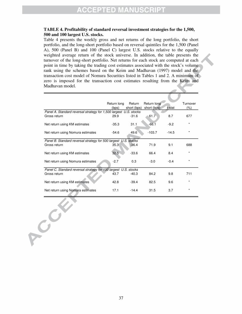
We first consider the results for a standard reversal strategy using the 1,500 largest
U.S. stocks in Panel A of Table 4. Consistent with most of the literature we find that
this strategy yields extremely large gross returns. More specifically, a reversal
investment strategy that is long in the 20 percent stocks with the lowest one-week
returns and short in the 20 percent with the highest returns earns a gross return of 61.7
basis points per week.
However, at the same time the reversal strategy has an extremely high
portfolio turnover of 677 percent per week.4 We find that the average holding period
of a stock is less than three days. Once trading costs are taken into account the
profitability of the reversal strategy completely diminishes. When we take Keim and
Madhavan (1997) trading cost estimates, we document a net return of minus 66.1
4 The maximum turnover of a long-short portfolio is 400 percent per day.

15
basis points per week. And when we use the Nomura cost estimates, we even find a
return of minus 103.7 basis points per week. These results are consistent with the
findings of Avramov, Chordia and Goyal (2006).
One of the most notable observations in the previous section was that there is a
highly non-linear relation between market capitalization/trading volume and trading
costs such that the smallest and least liquid stocks are disproportionally expensive to
trade. Especially since these stocks generally have the highest volatility and therefore
have the greatest probability to end up in the extreme quantiles when stocks are
ranked on past returns, a long-short reversal portfolio is typically invested in the
stocks that are the most expensive to trade. While some studies report that stock
anomalies are typically stronger among small cap stocks, one may wonder if the
potentially higher returns of small cap stocks compensate for the higher trading costs
of these stocks.
To investigate the impact of including small cap stocks, we consider the results
for the 500 and 100 largest U.S. stocks in Panels B and C of Table 4, respectively.
Interestingly, the reversal strategies for the largest 500 and 100 stocks earn slightly
higher returns than the reversal strategy for the largest 1,500 stocks. Moreover, it
appears that the impact of trading costs on the profitability of the strategy is much
lower for our samples of large cap stocks. Given the large number of negative cost
estimates we found using the Keim and Madhavan (1997) model for the largest 500
stocks, it is not surprising to see that the net return of the reversal strategy computed
using these cost estimates are very close to the strategy’s gross return since we impose
minimum trading costs of zero. However, also when we use the trading cost estimates
of Nomura, it appears that trading costs have a much smaller impact on reversal
profits once small cap stocks are excluded. The net return of minus 3.0 basis points

16
per week of the strategy for the 500 largest stocks indicates that trading costs consume
roughly 75 basis points of the strategy’s gross return. For the 100 largest stocks this
figure is 53 basis points. For our sample of the 1,500 largest stocks trading impact is
more than three times larger at 165 basis points.
The results from this analysis indicate that reversal profits are also observed
among the largest stocks. In fact, reversal profits appear to be the highest among this
group of stocks. Our finding that reversal strategies can yield a significant return of
more than 30 basis points per week net of trading costs presents a serious challenge to
standard rational asset pricing model and has important implications for the practical
implementation of reversal investment strategies. The key lesson is that investors
striving to earn superior returns by engaging in reversal trading are more likely to
realize their objectives by trading in liquid stocks with relatively low transaction
costs.
4.2. Reducing reversal strategies’ turnover by “smart” portfolio construction
Another important reason why trading costs have such a large impact on reversal
profits has to do with the way the reversal portfolios are typically constructed.
Reversal portfolios are constructed by taking a long position in losers and a short
position in winners. Then, at a pre-specified interval the portfolio is rebalanced and
stocks that are no longer losers are sold and replaced by newly bottom-ranked stocks.
And vice versa, stocks that are no longer winners are bought back and replaced by
newly top-ranked stocks. While this portfolio construction approach is standard in the
academic literature to investigate stock market anomalies, it is suboptimal when a
real-live investment strategy is evaluated and trading costs are taken into account.
Namely, replacing stocks that are no longer losers (winners) by newly bottom (top)-

17
ranked stocks only increases the profitability of reversal strategies if the difference in
expected return between the stocks is larger than the costs associated with the
transactions.
In many cases, however, the costs of the rebalances will be larger than the
incremental return that is earned by the stock replacements. For example, for our
universe of the 1,500 largest stocks we found that past loser stocks on average earn a
gross excess return of roughly 6 basis points over the subsequent day while stocks in
the next quintile earn 1 basis point. On average, loser (winner) stocks remain ranked
in the top (bottom) quintile for a period of three days. Consequently, replacing a stock
that moved from the top quintile to the second quintile only increases the profitability
of the reversal strategy if the costs of the buy and sell transactions are less than 15 [=
(6 - 1) * 3] basis points together. When we consider the trading cost estimates in
Tables 1 and 2, however, we see that single-trip costs are larger than 7.5 basis points
in many cases. Therefore a portfolio construction approach that directly sells (buys
back) stocks that are no longer losers (winners) is likely to generate excessive
turnover and unnecessarily high transaction costs.
A naive approach to cope with this problem would be to lower the rebalancing
frequency. However, with this approach one runs the risk to hold stocks that have
already reverted. Namely, a loser (winner) stock at a specific point in time might rank
among the winner (loser) stocks within the interval at which the portfolio is
rebalanced and might therefore have a negative (positive) expected return. In fact, the
portfolio weights of loser stocks that have reverted become larger and thereby
exacerbate this effect.
We propose a slightly more sophisticated approach that waits to sell (buy
back) stocks until they are ranked among the 50 percent of winner (loser) stocks

18
ranked on past return. These stocks are then replaced by the stocks with the lowest
(highest) past-week return at that time and not yet included in the portfolio. As a
consequence, this "smart" approach has a substantially lower turnover than the
standard approach to construct long-short reversal portfolios. It is important to note
that our “smart” approach holds the same number of stocks in the portfolio as the
standard approach, but that the holding period with the “smart” approach is flexible
for each stock with a minimum of one day and a maximum of theoretically infinity.
We now use the slightly more sophisticated portfolio construction approach
outlined above to evaluate reversal profits for our samples of the 1,500, 500, and 100
largest U.S. stocks. Our hypothesis is that trading costs can significantly be reduced
without giving up too much of the gross reversal profits when our slightly more
sophisticated portfolio construction algorithm is applied.
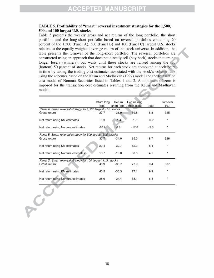
[INSERT TABLE 5 ABOUT HERE]
We first consider the results for our sample of the 1,500 largest stocks in Panel A of
Table 5. Indeed, the “smart” portfolio construction approach appears to successfully
reduce turnover and thereby the impact of trading costs on reversal profits. While the
turnover of the standard reversal strategy for the 1,500 largest stocks is 677 percent
per week, this figure is 325 percent for the “smart” approach. We find that the
effective holding period of a stock on average is approximately six days for this
strategy. And while trading costs, estimated using the Keim and Madhavan (1997)
model, consume 128 basis points of reversal gross returns of the standard reversal
strategy, this figure is 61 basis points for the “smart” approach. We find a similar
impact when we use the Nomura trading cost estimates. While trading costs consume
165 basis points for the standard reversal strategy, this figure is 77 basis points for the
“smart” approach. All in all, it appears that using a slightly more sophisticated
19
portfolio construction approach when engaging in short-term reversal strategies can
have a significant impact on trading costs.
Next, we consider the results for the 500 and 100 largest U.S. stocks in Panels
B and C of Table 5. Also for these samples we see that the “smart” portfolio
construction approach appears to successfully reduce turnover. More specifically,
while the standard reversal strategies have turnovers of 688 and 711 percent per week,
these figures are 326 and 337 percent for the “smart” reversal strategies applied on the
500 and 100 largest stocks, respectively. Interestingly, the gross returns of the “smart”
strategies are only marginally lower than the returns we observed earlier for the
standard reversal strategies. When net returns are computed using the Nomura model
we find that trading costs now consume only 34 basis points of the strategy’s gross
return for the 500 largest U.S. stocks. This figure is 75 basis points for the standard
reversal strategy. We observe a similar reduction for our sample of the 100 largest
U.S. stocks. The resulting reversal profits range between 30 and 50 basis points per
week and are highly significant from both a statistical as an economical point of
view.
4.3. Reversal profits in European markets
Proceeding further we evaluate reversal profits in European stocks markets. Only a
small number of studies have investigated short-term reversal strategies in non-US
equity markets. Chang, McLeavey and Rhee (1995) find abnormal profits of short-
term contrarian strategies in the Japanese stock market. Schiereck, DeBondt and
Weber (1999) and Hameed and Ting (2000) find the same in the German and
Malaysian stock markets, respectively. And Griffin, Kelly and Nardari (2010)
investigate reversal profits in 56 developed and emerging countries.

20
Because European markets are less liquid than the U.S. market we expect the
impact of trading costs on reversal profits to be larger in Europe. Using the
methodology outlined in the previous section, we construct quintile portfolios for the
1,000, 600 and 100 largest European stocks to compute the returns of long-short
reversal portfolios. Additionally, we apply the “smart” portfolio construction for these
stock samples. For all reversal strategies we compute gross returns, and returns net of
trading costs using the estimates from the Nomura model listed in Table 3. The results
of this analysis are presented in Table 6.
[INSERT TABLE 6 ABOUT HERE]
It appears that gross reversal profits are also very large in Europe and in the same
order of magnitude as in the U.S. However, as we expected, the impact of trading
costs appears to be larger in Europe. For our universes of the 1,000 and 600 largest
European stocks we do not find positive returns net of trading costs. Only when we
exclusively focus on the 100 largest stocks and apply the “smart” portfolio
construction, we document significantly positive net reversal profits up to 20 basis
points per week.
All in all, the European results exhibit the same features as our U.S. results:
once we move more towards the large cap segment of the market and limit turnover
by “smart” portfolio construction, reversal strategies yield significant returns net of
trading costs. At the same time, trading costs have a larger impact on reversal profits
in Europe than in the U.S.
5. Follow-up empirical analyses
5.1. Weekly rebalancing

21
In our first follow-up empirical analysis we evaluate a naive portfolio construction
approach that reduces the turnover of reversal strategies by decreasing the rebalancing
frequency to five days. All the other settings are exactly the same as with the standard
approach. As mentioned earlier, the main disadvantage of this approach compared to
the "smart" portfolio construction approach described in the previous section is that
one runs the risk to hold stocks that have already reverted. We evaluate this portfolio
construction approach for our samples of the largest 1,500, 500 and 100 largest U.S.
stocks. The results are in Table 7.
[INSERT TABLE 7 ABOUT HERE]
It appears that using a five-day rebalancing frequency indeed substantially lowers
portfolio turnover. For example, the turnover of the standard reversal strategy for the
1,500 largest stocks is 677 percent per week. This figure is 306 percent per week
using a five-day rebalancing frequency. Also for our samples of the largest 500 and
100 stocks, the turnover of reversal strategies that use a five-day rebalancing
frequency is less than half of the turnover of strategies that rebalance at a daily
frequency. As a consequence, the impact of trading costs is substantially lower for
these strategies. Nonetheless, the net returns of the weekly reversal strategy for the
1,500 largest stocks are significantly negative because the gross returns of the strategy
are also much lower than for the daily strategy. While the daily strategy yields a gross
return of 61.7 basis points per week, the weekly strategy yields only 41.2 basis points.
For our samples of the largest 500 and 100 stocks we observe similar effects: trading
costs become substantially lower when the rebalancing frequency is decreased to five
days, but so do gross returns. The effects seem to offset each other such that net
reversal profits remain in the same order of magnitude.

22
5.2. Subperiod analyses
We continue our empirical analysis by performing two subperiod analyses. First, we
investigate reversal profits over the most recent decade in our sample (i.e., January
2000 to December 2009). We conjecture that it might well be the case that the
decimalization of the quotation systems and the increase in stock trading volumes
have affected the profitability of reversal profits. Additionally, the Adaptive Market
Hypothesis of Lo (2004) states that the public dissemination of an anomaly may affect
its profitability. We conjecture that it could well be the case that increased investment
activities by professional investors such as hedge funds have arbitraged away a large
portion of the anomalous profits of reversal strategies after publications on the
reversal effect in the 1990s. The results of this analysis are presented in Panels A, B
and C in Table 8.
[INSERT TABLE 8 ABOUT HERE]
It appears that the net profitability of our “smart” reversal investment strategy is quite
constant over our sample period. For the 1,500 largest stocks, the “smart” reversal
strategy yields a negative net return of minus 27.9 basis points per week in the most
recent decade. For our sample of the 500 largest stocks, the net return decreased from
30.5 to 22.1 basis points per week. And for our sample of the largest 100 stocks, the
net return slightly increased from 53.1 basis points to 59.0 basis points per week.
In our second subperiod analysis we evaluate reversal profits when leaving out
the dotcom bubble years (i.e., January 1999 to December 2001) and the credit crisis
(i.e., January 2008 to December 2009) from our sample. Our concern is that the
trading cost models we employ underestimate costs during crises periods and reversal
profits are exacerbated. The results of this analysis are reported in Panels D, E, and F
of Table 8. Observing net reversal profits of minus 17.8, 23.2 and 34.8 basis points

23
per week for the 1,500, 500 and 100 largest U.S. stocks, respectively, we conclude
that the reversal profits are constant over time and also highly profitable during non-
crises periods.
5.3. “Smart” portfolio construction using alternative trade rules
Next we examine the sensitivity of our findings to alternate portfolio construction rule
choices. More specifically, we evaluate reversal profits for the 500 largest U.S. stocks
that sell (buy back) stocks once their rank on past-week return is above (below) the
30th (70th) percentile; the 40th (60th) percentile; the 60th (40th) percentile; the 70th
(30th) percentile; and the 80th (20th) percentile.
[INSERT TABLE 9 ABOUT HERE]
The results in Panel A of Table 9 point out that reducing portfolio turnover has a large
impact on net reversal profits. Once we require loser (winner) stocks with a rank
above (below) the 30th (70th) percentile to be sold (bought back), net reversal profits
become highly significant at 20.1 basis points per week. This compares to minus 3
basis points per week for the standard reversal strategy (see Table 4). While gross
returns become somewhat lower when turnover is reduced, the impact of trading costs
on performance becomes substantially smaller at the same time. The optimum in
terms of net return is reached using a trade rule that sells (buys back) stocks once their
rank on past-week return is above (below) the 70th (30th) percentile. Interestingly, it
appears that reversal profits are both statistically and economically highly significant
for all trade rules, ranging from 20.1 to 35.3 basis points per week. We can therefore
safely conclude that our findings are robust to our choice of trade rule.
5.4. Fama-French regressions

24
To investigate to which extent reversal profits can be attributed to exposures to
common risk factors we regress gross and net returns of the “smart” long-short
reversal portfolios for the largest 1,500, 500 and 100 U.S. stocks on the Fama-French
risk factors (French, 2010) for market, size and value [see, e.g., Fama and French
(1993, 1995, 1996)]:
(1) iitttti HMLbSMBbsRMRFbar ,321, ε++++= ,
where tir , is the return on reversal strategy i in month t, tRMRF , tSMB and tHML are
the returns on factor-mimicking portfolios for the market, size and value in month t,
respectively, a , 1b , 2b and 3b are parameters to be estimated, and ti,ε is the residual
return of strategy i in month t. The coefficient estimates and adjusted R-squared
values from these regressions are listed in Table 10.
[INSERT TABLE 10 ABOUT HERE]
Panel A presents the results for the 1,500 largest U.S. stocks, Panel B presents the
results for the 500 largest U.S. stocks, and Panel C presents the results for the 100
largest U.S. stocks. In all cases the explanatory power of the Fama-French risk factors
is very small. The highest adjusted R-squared value we observe is 5 percent. We
conclude that reversal profits are unrelated to exposures to common risk factors.
6. Implications for explanations for reversal effects
Our findings have important implications for explanations that have been put forward
in the literature to explain the reversal anomaly. Short-term stock reversals are
sometimes regarded as evidence that the market lacks sufficient liquidity to offset
price effects caused by unexpected buying and selling pressure and that market
makers set prices in part to control their inventories. Grossman and Miller (1988) and
Jegadeesh and Titman (1995b) argue that the reversals are induced by inventory

25
imbalances by market makers and the contrarian profits are a compensation for
bearing inventory risks. Related to this stream of literature, Madhavan and Smidt
(1993), Hasbrouck and Sofianos (1993), Hansch, Naik and Viswanathan (1998), and
Hendershott and Seasholes (2006) find that prices quoted by dealers are inversely
related to their inventory supporting the notion that dealers actively manage their
inventories. This liquidity explanation projects that reversals should have become
smaller over time since market liquidity dramatically increased. It also predicts that
reversals are stronger for small cap stocks than large cap stocks that typically have
lower turnover. In fact, under the liquidity hypothesis reversals may even not be
present among large cap stocks at all. However, our findings that net reversal profits
are large and positive for the 500 and 100 largest U.S. stocks and did not diminish
over the second decade in our sample rules out this explanation.
Another explanation for reversal effects that has been put forward in the
literature is from Lo and MacKinlay (1990) and Boudoukh, Richardson and Whitelaw
(1994) who note that nonsynchronous trading contributes to contrarian profits. This
explanation assumes information diffuses gradually in financial markets and that large
cap stocks react more quickly to information than small cap stocks that are covered by
fewer analysts. As a consequence of this, the returns of large cap stocks might lead the
returns of small cap stocks. However, our finding that reversal profits are smaller for
the 1,500 largest U.S. stocks than for the 500 and 100 largest stocks is inconsistent
with this explanation since nonsynchronous trading predicts a size-related lead-lag-
effect in stock returns and higher reversal profits among small cap stocks.
The only explanation that has been put forward in the literature whose
projections are not inconsistent with our findings is the behavioural explanation that
market prices tend to overreact to information in the short run [see, e.g., Jegadeesh

26
and Titman (1995a)]. It should be stressed that our study does not provide any direct
evidence supporting this behavioural hypothesis. Of course, it is not our goal to
explain the reversal effect in this study; our main point is to show that reversal profits
are present after trading costs. Nonetheless, we believe that our results help to better
understand the reversal anomaly since it rules out several competing explanations that
have been put forward in the literature.
7. Summary and concluding comments
This paper shows that the finding that trading costs prevent profitable execution of
reversal investment strategies can largely be attributed to excessively trading in small
cap stocks. Excluding small cap stocks and applying a slightly more sophisticated
portfolio construction approach to reduce turnover when engaging in reversal trading
has a tremendous impact on the returns that reversal investment strategies deliver net
of transaction costs. Our finding that reversal strategies generate 30 to 50 basis points
per week net of transaction costs poses a serious challenge to standard rational asset
pricing models and has important implications for the practical implementation of
reversal investment strategies. Our results also have important implications for several
explanations that have been put forward in the literature to explain the reversal
anomaly.
Another important issue that came to light in this study is that trading cost
estimates of the Keim and Madhavan (1997) model that are typically used in this
stream of literature to evaluate the profitability of trading strategies net of transaction
costs should be interpreted with caution in some cases. More specifically, it seems
that cost estimates of this model are systematically biased downwards and can even
become negative. The comprehensive overview presented in this study on trading

27
costs estimates resulting from the proprietary transaction cost model of Nomura
Securities provides opportunities for future research to re-evaluate the profitability of
investment strategies based on well-documented anomalies.

28
Appendix
This appendix describes the Keim and Madhavan (1997) and the Nomura models we
use throughout this study to estimate trading costs.
A. Keim and Madhavan (1997) model
As Avramov, Chordia and Goyal (2006) do in their study, we employ the regression
results of Keim and Madhavan to estimate the transaction costs involved with reversal
investment strategies. Using the results in Table 5 of Keim and Madhavan (1997) we
obtain our estimates of buyer and seller trading costs:
(2) ���
����
�+−++=
iii
i
iNASDAQ
iBuy
PmcapTrsize
mcapDC
1807.13log084.0
1092.0336.0767.0ˆ
(3) ���
����
�+−++=
iii
i
iNASDAQ
iSell
PmcapTrsize
mcapDC
1537.6log059.0
1214.0058.0505.0ˆ
where iBuyC and i
SellC are the estimated total trading costs for stock i in percent for
either a buyer-initiated or seller-initiated order, respectively. iNASDAQD is equal to one
if stock i is a NASDAQ-traded stock and zero if stock i is traded on NYSE or AMEX,
imcap is the market value outstanding of stock i, iTrsize is the trade size of stock i,
and iP is the price per share of stock i. For our long portfolios we use iBuyC to open
the positions in the component stocks and iSellC to close the positions, vice versa for
the short portfolios. Keim and Madhavan estimate the trading costs for 21 institutions
from January 1991 through March 1993 using 62,333 trades.

29
B. Nomura model for trading costs
The variables that are assumed to determine trading costs in the model developed by
Nomura are spread, trade size, volume and volatility:
(4) iiii
ii volatilitybTrsizevolume
bspreadbaC ε++++= 3221
1ˆ
where ispread is the average bid-ask spread of stock i over the trading day, ivolume
is the total executed volume for stock i over the trading day, iTrsize is the trade size
of stock i, and ivolatility the intra-day return volatility of stock i over the trading day.
The Nomura trading cost model is calibrated in every quarter over the period 1995 to
2009. For each calibration, actual order flows in the previous 12 months for
approximately 500,000 executed trades per time are used from the trading platform
formerly owned by Lehman Brothers. Consistent with the approach of Keim and
Madhavan (1997), the model of Nomura also adjusts for the relevant exchange by
estimating the model coefficients per region and exchange [Tse and Devos (2004) and
Gajewskia and Gresse (2007) report differences in trading costs between exchanges].
The model developed by Nomura estimates transaction costs by decomposing
them into three components. The first component is the instantaneous impact due to
crossing the bid-ask spread. The second component is the permanent impact which is
the change in market equilibrium price due to executing a trade. Finally, the third
component is the temporary impact which refers to a temporary movement of price
away from equilibrium price because of short-term imbalances in supply and demand.
The model does not take opportunity costs into account that result from unfilled
trades.

30
References
Amihud, Y., 2002. Illiquidity and stock returns: Cross-section and time-series effects.
Journal of Financial Markets 5, 31-56.
Avramov, D., Chordia, T., Goyal, A., 2006. Liquidity and autocorrelations in
individual stock returns. Journal of Finance 61, 2365-2394.
Ball, R., Kothari, S.P., Wasley, C.E., 1995. Can we implement research on stock
trading rules? Journal of Portfolio Management 21, 54-63.
Boudoukh, J., Richardson, M.P., Whitelaw, R.F., 1994. Tale of three schools: Insights
on autocorrelations of short-horizon stock returns. Review of Financial Studies 7,
539-573.
Chan, W.S., 2003. Stock price reaction to news and no-news: Drift and reversal after
headlines. Journal of Financial Economics 70, 223-260.
Chang, R.P., McLeavey, D.W., Rhee S.G., 1995. Short-term abnormal returns of the
contrarian strategy in the Japanese stock market. Journal of Business Finance and
Accounting 22, 1035-1048.
Chordia, T., Goyal, A., Sadka, G., Sadka, R., Shivakumar, L., 2009. Liquidity and the
post-earnings-announcement drift. Financial Analysts Journal 65, 18-32.
Conrad, J.S., Gultekin, M., and Kaul, M., 1997. Profitability of short-term contrarian
strategies: implications for market efficiency. Journal of Business and Economic
Statistics 15, 379-386.
Fama, E.F., 1965. The behavior of stock market prices. Journal of Business 38, 34-
105.
Fama, E.F., French, K.R., 1993. Common risk factors in the returns on stocks and
bonds. Journal of Financial Economics 33, 3-56.

31
Fama, E.F., French, K.R., 1995. Size and book-to-market factors in earnings and
returns. Journal of Finance 50, 131-155.
Fama, E.F., French, K.R., 1996. Multifactor explanations of asset pricing anomalies.
Journal of Finance 1, 55-84.
French, K.R., Fama-French Factors, 2010. Retrieved July 2010 from
http://mba.tuck.dartmouth.edu/pages/faculty/ken.french/data_library.html
Gajewskia, J., Gresse, C., 2007. Centralised order books versus hybrid order books: A
paired comparison of trading costs on NSC (Euronext Paris) and SETS (London Stock
Exchange). Journal of Banking and Finance 31, 2906-2924.
Gutierrez Jr., R.C., Kelley, E.K., 2008. The long-lasting momentum in weekly
returns. Journal of Finance 63, 415-447.
Griffin, J.M., Kelly, P.J., Nardari, F., 2010. Do market efficiency measures yield
correct inferences? A comparison of developed and emerging markets. Review of
Financial Studies 23, 3225-3277.
Grossman, S., Miller, M., 1988. Liquidity and market structure. Journal of Finance 43,
617-633.
Hameed, A., Ting, S., 2000. Trading volume and short-horizon contrarian profits:
Evidence from Malaysian stock market. Pacific-Basin Finance Journal 8, 67-84.
Hansch, O., Naik, N.Y., Viswanathan, S. 1998. Do inventories matter in dealership
markets? Evidence from the London Stock Exchange. Journal of Finance 53, 1623-
1656.
Hasbrouck, J., Sofianos, G., 1993. The trades of market makers: An empirical analysis
of NYSE specialists. Journal of Finance 48, 1565–1593.

32
Hendershott, T., Seasholes, M.S., 2006. Specialist inventories and stock prices.
American Economic Review Papers and Proceedings 97, 210-214.
Jegadeesh, N., 1990. Evidence of predictable behavior of security returns. Journal of
Finance 45, 881-898.
Jegadeesh, N., Titman, S., 1995a. Overreaction, delayed reaction, and contrarian
profits. Review of Financial Studies 8, 973-993.
Jegadeesh, N., Titman, S., 1995b. Short-horizon return reversals and the bid-ask
spread. Journal of Financial Intermediation 4, 116-132.
Kaul, G., Nimalendran, M., 1990. Price reversals: Bid-ask errors or market
overreaction? Journal of Financial Economics 28, 67-93.
Keim, D.B., Madhavan, A., 1997. Transaction costs and investment style: An inter-
exchange analysis of institutional equity trades. Journal of Financial Economics 46,
265-292.
Korajczyk, R., Sadka, R. 2004. Are momentum profits robust to trading costs? Journal
of Finance 59, 1039-1082.
Lehmann, B., 1990. Fads, martingales, and market efficiency. Quarterly Journal of
Economics 105, 1-28.
Lesmond, D.A., Schill, M. J., Zhou, C., 2004. The illusory nature of momentum
profits. Journal of Financial Economics 71, 349-380.
Lo, A.W., 2004. The adaptive markets hypothesis: Market efficiency from an
evolutionary perspective. Journal of Portfolio Management 30, 15-29.
Lo, A.W., MacKinlay, A.C., 1990. When are contrarian profits due to stock market
overreaction? Review of Financial Studies 3, 175-205.

33
Madhavan, A., Smidt, S., 1993. An analysis of changes in specialist inventories and
quotations. Journal of Finance 48, 1595-1628.
Rosenberg, B., Reid, K., Lanstein, R., 1985. Persuasive evidence of market
inefficiency. Journal of Portfolio Management 11, 9-17.
Ro�u, I., 2009. A dynamic model of the limit order book. Review of Financial Studies
22, 4601-4641.
Schiereck, D., DeBondt, W., Weber, M., 1999. Contrarian and momentum strategies
in Germany. Financial Analysts Journal 55, 104-116.
Subrahmanyam, A., 2005. Distinguishing between rationales for short-horizon
predictability of stock returns. Financial Review 40, 11-35.
Tse, Y., Devos, E., 2004. Trading costs, investor recognition and market response: An
analysis of firms that move from the Amex (Nasdaq) to Nasdaq (Amex). Journal of
Banking and Finance 28, 63-83.

34
TABLE 1. Transaction cost estimates for the 1,500 largest U.S. stocks. Table 1 presents an overview of the single-trip transaction cost estimates in basis points for volume deciles of our sample of the 1,500 largest U.S. stocks resulting from the Keim and Madhavan model (Panel A) and the estimates for volume deciles of S&P1500 stocks we received from Nomura Securities (Panel B). Volume deciles are based on stocks' three-month median trading volumes. It is assumed that the trades are closed within one day and the trade size is one million per stock by the end of 2009. The trade size is deflated back in time with 10 percent per annum.
Volume Decile 19
90
1991
1992
1993
1994
1995
1996
1997
1998
1999
2000
2001
2002
2003
2004
2005
2006
2007
2008
2009
Ave
rage
Panel A. Keim-Madhaven average buy and sellD1 (bottom) 71 78 47 28 29 27 21 12 13 18 21 26 30 29 13 12 10 11 38 63 30D2 82 74 53 32 33 30 20 10 14 20 27 29 38 36 15 13 9 8 37 66 32D3 64 72 51 32 30 25 18 11 15 19 24 24 39 35 19 10 7 7 40 61 30D4 56 53 38 30 32 25 15 12 14 18 21 29 42 32 19 15 6 8 34 58 28D5 48 39 32 30 25 22 15 9 11 17 15 27 43 38 15 16 6 4 24 37 24D6 38 29 23 22 20 14 10 8 8 11 15 23 41 26 14 11 6 1 16 34 18D7 24 20 18 13 14 8 6 1 4 5 6 15 26 22 8 2 2 -6 15 28 11D8 16 11 9 8 4 4 1 -3 -5 -6 0 13 14 10 2 -6 -11 -14 7 21 4D9 0 -3 -5 -5 -2 -6 -6 -11 -12 -13 -10 0 3 0 -9 -17 -16 -21 -5 8 -7D10 (top) -20 -20 -19 -19 -17 -19 -22 -26 -28 -31 -25 -14 -5 -11 -17 -25 -26 -31 -21 -15 -20
Panel B. Nomura buy or sellD1 (bottom) 86 77 83 75 73 54 52 66 53 76 65 88 80 76 76 65 53 41 51 70 68D2 72 60 60 55 51 34 27 35 31 65 67 61 56 50 41 30 24 20 25 50 46D3 58 50 45 41 38 23 19 22 23 47 47 37 30 24 20 17 15 14 17 33 31D4 48 41 36 30 30 17 12 18 18 30 28 23 20 17 14 13 12 11 13 23 23D5 41 34 30 26 25 15 14 14 17 21 19 16 15 13 12 11 10 9 11 17 19D6 33 26 22 21 20 13 13 12 14 16 14 13 12 11 10 9 9 8 9 14 15D7 26 23 21 18 17 11 17 11 11 13 11 10 9 9 8 8 8 7 8 11 13D8 22 20 18 16 14 10 17 13 10 11 9 8 8 8 7 7 6 6 6 9 11D9 17 15 14 13 13 9 11 11 10 9 7 7 7 6 6 6 6 5 6 7 9D10 (top) 13 14 14 13 13 10 9 8 8 7 5 5 5 5 5 5 5 5 5 5 8

35
TABLE 2. Transaction cost estimates for the 500 largest U.S. stocks. Table 2 presents an overview of the single-trip transaction cost estimates in basis points for volume deciles of our sample of the 500 largest U.S. stocks resulting from the Keim and Madhavan model (Panel A) and the estimates for volume deciles of S&P500 stocks we received from Nomura Securities (Panel B). Volume deciles are based on stocks' three-month median trading volumes. It is assumed that the trades are closed within one day and the trade size is one million USD per stock by the end of 2009. The trade size is deflated back in time with 10 percent per annum.
Volume Decile 19
90
1991
1992
1993
1994
1995
1996
1997
1998
1999
2000
2001
2002
2003
2004
2005
2006
2007
2008
2009
Ave
rage
Panel A. Keim-Madhaven average buy and sellD1 (bottom) 14 6 2 1 8 8 2 -4 0 6 9 8 4 3 -4 -9 -11 -16 -5 51 4D2 14 10 3 1 3 0 -1 -8 -8 -5 -4 -3 5 7 -3 -9 -12 -16 -4 46 1D3 12 6 5 1 1 -2 -8 -11 -10 -8 -6 -3 3 -1 -8 -13 -16 -19 -2 40 -2D4 8 7 3 0 0 -2 -7 -11 -12 -11 -11 -6 2 -1 -11 -15 -19 -19 -6 39 -4D5 9 5 1 -2 -2 -3 -10 -12 -14 -15 -12 -10 0 -1 -11 -16 -21 -21 -10 28 -6D6 6 1 -4 -7 -3 -7 -11 -15 -16 -16 -17 -11 2 -3 -14 -21 -18 -23 -7 26 -8D7 1 -5 -6 -8 -5 -10 -12 -17 -17 -16 -20 -8 1 -2 -15 -16 -18 -22 -11 15 -10D8 -7 -10 -9 -10 -9 -12 -15 -17 -19 -24 -21 -9 0 0 -14 -16 -21 -28 -8 16 -12D9 -12 -10 -13 -15 -14 -17 -21 -25 -27 -30 -29 -16 -9 -12 -14 -24 -22 -27 -17 2 -18D10 (top) -24 -25 -27 -24 -24 -27 -29 -34 -38 -39 -38 -19 -4 -22 -27 -30 -32 -34 -24 -16 -27
Panel B. Nomura buy or sellD1 (bottom) 23 15 13 15 22 31 25 24 23 23 34 36 34 38 40 28 19 15 13 21 25D2 12 11 10 12 16 22 13 14 16 27 26 20 17 17 14 11 10 9 10 14 15D3 11 10 9 11 14 14 11 17 14 16 16 13 12 12 10 9 9 8 8 12 12D4 10 9 9 11 12 12 12 12 12 13 12 11 10 10 9 8 8 7 7 11 10D5 9 9 8 10 11 12 12 11 10 11 10 9 9 9 8 7 7 6 7 9 9D6 8 8 8 9 10 13 12 11 10 10 9 8 8 8 7 7 6 6 6 9 9D7 8 8 8 9 9 11 11 10 9 11 8 7 7 7 7 6 6 6 6 8 8D8 8 8 7 8 9 11 11 10 10 9 7 6 7 7 6 6 6 5 6 7 8D9 7 7 7 7 9 10 9 9 9 8 6 6 6 6 6 5 5 5 5 6 7D10 (top) 7 7 6 7 8 10 9 8 8 7 4 5 5 5 5 5 5 4 4 5 6

36
TABLE 3. Transaction cost estimates for the 1,000 and 600 largest European stocks. Table 3 presents an overview of the single-trip transaction cost estimates in basis points for volume deciles of our sample of the 1,000 (Panel A) and 600 (Panel B) largest European stocks resulting from the estimates for volume deciles we received from Nomura Securities. Volume deciles are based on stocks' three-month median trading volumes. It is assumed that the trades are closed within one day and the trade size is one million per stock by the end of 2009. The trade size is deflated back in time with 10 percent per annum.
Volume Decile 19
95
1996
1997
1998
1999
2000
2001
2002
2003
2004
2005
2006
2007
2008
2009
Ave
rage
Panel A. 1,000 largest European stocksD1 (bottom) 75 75 77 77 77 71 75 77 79 72 74 76 71 79 88 76D2 64 64 57 62 68 64 71 74 75 68 62 53 48 71 82 66D3 46 46 43 48 51 54 60 63 63 48 48 39 35 56 75 52D4 38 37 35 41 41 46 50 53 52 38 42 32 30 46 66 43D5 33 31 31 34 35 40 44 43 43 31 35 27 26 38 56 37D6 27 28 27 28 31 34 35 36 33 27 30 24 24 32 46 31D7 24 24 24 25 26 27 28 29 27 23 25 22 23 28 40 26D8 22 22 22 23 23 22 23 23 23 21 22 20 20 25 31 23D9 22 21 20 21 21 19 20 20 20 19 20 19 19 21 25 20D10 (top) 21 20 20 20 19 17 19 19 19 18 19 18 18 20 22 19
Panel B. 600 largest European stocksD1 (bottom) 72 72 69 68 75 64 71 72 72 66 63 57 50 66 80 68D2 54 51 44 50 53 55 61 62 62 48 46 33 30 48 67 51D3 36 36 34 38 39 44 45 49 47 31 36 27 25 35 51 38D4 30 29 29 30 32 34 36 35 39 27 29 25 24 30 42 31D5 26 26 26 27 28 29 30 30 32 23 26 23 22 27 39 28D6 23 24 24 25 25 24 25 26 26 21 23 21 22 26 34 25D7 22 22 22 22 23 22 22 22 23 20 21 20 20 23 28 22D8 22 21 21 22 21 19 20 20 21 19 20 19 18 21 25 21D9 21 20 19 20 20 18 19 19 20 19 19 19 18 20 23 20D10 (top) 21 20 18 19 18 16 19 19 19 18 18 18 17 19 21 19
37
TABLE 4. Profitability of standard reversal investment strategies for the 1,500, 500 and 100 largest U.S. stocks. Table 4 presents the weekly gross and net returns of the long portfolio, the short portfolio, and the long-short portfolio based on reversal quintiles for the 1,500 (Panel A), 500 (Panel B) and 100 (Panel C) largest U.S. stocks relative to the equally weighted average return of the stock universe. In addition, the table presents the turnover of the long-short portfolio. Net returns for each stock are computed at each point in time by taking the trading cost estimates associated with the stock’s volume rank using the schemes based on the Keim and Madhavan (1997) model and the transaction cost model of Nomura Securities listed in Tables 1 and 2. A minimum of zero is imposed for the transaction cost estimates resulting from the Keim and Madhavan model.
Return long (bps)
Return short (bps)
Return long-short (bps) t-stat
Turnover (%)
Panel A. Standard reversal strategy for 1,500 largest U.S. stocksGross return 29.9 -31.6 61.7 8.7 677
Net return using KM estimates -35.3 31.1 -66.1 -9.2 "
Net return using Nomura estimates -54.6 49.6 -103.7 -14.5 "
Panel B. Standard reversal strategy for 500 largest U.S. stocksGross return 35.3 -36.4 71.9 9.1 688
Net return using KM estimates 32.5 -33.6 66.4 8.4 "
Net return using Nomura estimates -2.7 0.3 -3.0 -0.4 "
Panel C. Standard reversal strategy for 100 largest U.S. stocksGross return 43.7 -40.3 84.2 9.8 711
Net return using KM estimates 42.8 -39.4 82.5 9.6 "
Net return using Nomura estimates 17.1 -14.4 31.5 3.7 "
38
TABLE 5. Profitability of “smart” reversal investment strategies for the 1,500, 500 and 100 largest U.S. stocks. Table 5 presents the weekly gross and net returns of the long portfolio, the short portfolio, and the long-short portfolio based on reversal portfolios containing 20 percent of the 1,500 (Panel A), 500 (Panel B) and 100 (Panel C) largest U.S. stocks relative to the equally weighted average return of the stock universe. In addition, the table presents the turnover of the long-short portfolio. The reversal portfolios are constructed using an approach that does not directly sell (buy back) stocks that are no longer losers (winners), but waits until these stocks are ranked among the top (bottom) 50 percent of stocks. Net returns for each stock are computed at each point in time by taking the trading cost estimates associated with the stock’s volume rank using the schemes based on the Keim and Madhavan (1997) model and the transaction cost model of Nomura Securities listed in Tables 1 and 2. A minimum of zero is imposed for the transaction cost estimates resulting from the Keim and Madhavan model.
Return long (bps)
Return short (bps)
Return long-short (bps) t-stat
Turnover (%)
Panel A. Smart reversal strategy for 1,500 largest U.S. stocksGross return 27.7 -31.9 59.8 8.8 325
Net return using KM estimates -2.9 -1.4 -1.5 -0.2 "
Net return using Nomura estimates -10.9 6.8 -17.6 -2.6 "
Panel B. Smart reversal strategy for 500 largest U.S. stocksGross return 30.7 -34.0 65.0 8.7 326
Net return using KM estimates 29.4 -32.7 62.3 8.4 "
Net return using Nomura estimates 13.7 -16.8 30.5 4.1 "
Panel C. Smart reversal strategy for 100 largest U.S. stocksGross return 40.9 -36.7 77.9 9.4 337
Net return using KM estimates 40.5 -36.3 77.1 9.3 "
Net return using Nomura estimates 28.6 -24.4 53.1 6.4 "

39
TABLE 6. Profitability of reversal investment strategies for the 1,000, 600 and 100 largest European stocks. Table 6 presents the weekly gross and net returns of the long portfolio, the short portfolio, and the long-short portfolio based on reversal strategies for the 1,000, 600 and 100 largest European stocks relative to the equally weighted average return of the stock universe. In addition, the table presents the turnover of the long-short portfolio. Net returns for each stock are computed at each point in time by taking the trading cost estimates associated with the stock’s volume rank using the schemes based on the transaction cost model of Nomura Securities listed in Table 3. Panels A, C and E present the results using a standard portfolio construction approach that is long (short) in the 20 percent of stocks with the lowest (highest) returns over the past week. Panels B, D and E show the results for a slightly more sophisticated portfolio construction approach that does not directly sell (buy back) stocks that are no longer losers (winners), but waits until these stocks are ranked among the top (bottom) 50 percent of stocks.
Return long (bps)
Return short (bps)
Return long-short (bps) t-stat
Turnover (%)
Panel A. Standard reversal strategy for 1,000 largest European stocksGross return 24.6 -25.3 50.0 7.7 672
Net return using Nomura estimates -113.4 106.5 -217.5 -33.4 "
Panel B. Smart reversal strategy for 1,000 largest European stocksGross return 28.2 -27.6 56.0 9.0 319
Net return using Nomura estimates -36.0 36.4 -72.1 -11.6 "
Panel C. Standard reversal strategy for 600 largest European stocksGross return 34.3 -34.6 69.2 9.6 683
Net return using Nomura estimates -81.3 76.8 -156.9 -21.8 "
Panel D. Smart reversal strategy for 600 largest European stocksGross return 35.0 -34.2 69.5 10.0 323
Net return using Nomura estimates -18.6 19.8 -38.3 -5.5 "
Panel E. Standard reversal strategy for 100 largest European stocksGross return 48.0 -48.1 96.5 9.8 700
Net return using Nomura estimates -24.9 22.9 -47.7 -4.9 "
Panel F. Smart reversal strategy for 100 largest European stocksGross return 46.3 -43.8 90.5 9.5 332
Net return using Nomura estimates 11.9 -9.7 21.6 2.3 "

40
TABLE 7. Profitability of reversal investment strategies using a five-day rebalancing frequency. Table 7 presents the weekly gross and net returns of the long portfolio, the short portfolio, and the long-short portfolio based on reversal quintiles using a five-day rebalancing frequency for the 1,500 (Panel A), 500 (Panel B) and 100 (Panel C) largest U.S. stocks. In addition, the table presents the turnover of the long-short portfolio. Net returns for each stock are computed at each point in time by taking the trading cost estimates associated with the stock’s volume rank using the schemes based on the transaction cost model of Nomura Securities listed in Tables 1 (for the 1,500 largest U.S. stocks) and 2 (for the 500 and 100 largest U.S. stocks).
Return long (bps)
Return short (bps)
Return long-short (bps) t-stat
Turnover (%)
Panel A. Standard reversal strategy for 1,500 largest U.S. stocks with a 5-day rebalancing frequencyGross return 18.6 -22.5 41.2 7.3 306
Net return using Nomura estimates -17.6 13.9 -31.4 -5.6 "
Panel B. Standard reversal strategy for 500 largest U.S. stocks with a 5-day rebalancing frequencyGross return 20.2 -23.7 44.0 7.1 310
Net return using Nomura estimates 3.5 -7.1 10.6 1.7 "
Panel C. Standard reversal strategy for 100 largest U.S. stocks with a 5-day rebalancing frequencyGross return 25.3 -26.7 52.2 7.9 315
Net return using Nomura estimates 13.7 -15.3 29.0 4.4 "

41
TABLE 8. Profitability of reversal investment strategies over subperiods Table 8 presents the weekly gross and net returns of the long portfolio, the short portfolio, and the long-short portfolio based on a reversal strategy over the period January 2000 to December 2009 (Panels A, B and C) and over our full sample period excluding the dot-com bubble from January 1999 to December 2001 and the credit crisis from January 2008 to December 2009 (Panels D, E and F). In addition, the table presents the turnover of the long-short portfolio. The reversal portfolios are constructed using an approach that does not directly sell (buy back) stocks that are no longer losers (winners), but waits until these stocks are ranked among the top (bottom) 50 percent of stocks. Net returns for each stock are computed at each point in time by taking the trading cost estimates associated with the stock’s volume rank using the schemes based on the transaction cost model of Nomura Securities listed in Tables 1 and 2.
Return long (bps)
Return short (bps)
Return long-short (bps) t-stat
Turnover (%)
Panel A. Smart reversal strategy for 1,500 largest U.S. stocks over the period 2000 to 2009Gross return 10.5 -22.6 33.2 2.7 317
Net return using Nomura estimates -19.4 8.5 -27.9 -2.3 "
Panel B. Smart reversal strategy for 500 largest U.S. stocks over the period 2000 to 2009Gross return 22.2 -30.7 53.0 4.0 320
Net return using Nomura estimates 7.1 -14.9 22.1 1.7 "
Panel C. Smart reversal strategy for 100 largest U.S. stocks over the period 2000 to 2009Gross return 40.0 -38.3 78.6 5.5 329
Net return using Nomura estimates 30.3 -28.5 59.0 4.1 "
Panel D. Smart reversal strategy for 1,500 largest U.S. stocks during non-crises periodsGross return 29.1 -31.8 61.1 12.1 325
Net return using Nomura estimates -10.4 7.4 -17.8 -3.5 ''
Panel E. Smart reversal strategy for 500 largest U.S. stocks during non-crises periodsGross return 27.5 -29.6 57.3 10.6 326
Net return using Nomura estimates 10.6 -12.6 23.2 4.3 ''
Panel F. Smart reversal strategy for 100 largest U.S. stocks during non-crises periodsGross return 31.9 -28.4 60.4 9.6 337
Net return using Nomura estimates 19.1 -15.7 34.8 5.5 ''

42
TABLE 9. “Smart” portfolio construction using alternative trade rules. Table 9 presents the weekly gross and net returns of the long portfolio, the short portfolio, and the long-short portfolio based on reversal strategies relative to the equally weighted average return of the stock universe. In addition, the table presents the turnover of the long-short portfolio. The reversal portfolios are constructed using an approach that does not directly sell (buy back) stocks that are no longer losers (winners), but waits until these stocks are ranked above (below) the 30th (70th) percentile (Panel A); the 40th (60th) percentile (Panel B); the 60th (40th) percentile (Panel C); the 70th (30th) percentile (Panel D); and the 80th (20th) percentile (Panel E). Net returns for each stock are computed at each point in time by taking the trading cost estimates associated with the stock’s volume rank using the schemes based on the transaction cost model of Nomura Securities listed in Table 2.
Return long (bps)
Return short (bps)
Return long-short (bps) t-stat
Turnover (%)
Panel A. Smart reversal strategy for 500 largest U.S. U.S. stocks using 30/70 trade ruleGross return 34.0 -37.2 71.5 9.1 479
Net return using Nomura estimates 8.1 -11.9 20.1 2.6 "
Panel B.Smart reversal strategy for 500 largest U.S. U.S. stocks using 40/60 trade ruleGross return 32.1 -35.8 68.2 8.9 387
Net return using Nomura estimates 11.5 -15.4 27.0 3.5 "
Panel C. Smart reversal strategy for 500 largest U.S. U.S. stocks using 60/40 trade ruleGross return 30.9 -33.0 64.1 8.9 275
Net return using Nomura estimates 16.7 -18.5 35.2 4.9 "
Panel D.Smart reversal strategy for 500 largest U.S. U.S. stocks using 70/30 trade ruleGross return 28.1 -30.5 58.7 8.6 225
Net return using Nomura estimates 16.7 -18.6 35.3 5.2 "
Panel E. Smart reversal strategy for 500 largest U.S. U.S. stocks using 80/20 trade ruleGross return 24.3 -27.3 51.7 8.2 170
Net return using Nomura estimates 15.8 -18.3 34.2 5.4 "

43
TABLE 10. Fama-French regressions. Table 10 present the coefficient estimates and adjusted R-squared values of Fama-French regressions of weekly gross and net returns of the long-short portfolio based on reversal portfolios containing 20 percent of the 1,500 (Panel A), 500 (Panel B) and 100 (Panel C) largest U.S. stocks on the Fama-French risk factors (French, 2010) for market, size and value [see, e.g., Fama and French (1993, 1995, 1996)]: (1) iitttti HMLbSMBbsRMRFbar ,321, ε++++= ,
where tir , is the return on reversal strategy i in month t, tRMRF , tSMB and tHML are the returns on factor-mimicking portfolios for the market, size and value in month t, respectively, a , 1b , 2b and 3b are parameters to be estimated, and ti,ε is the residual return of strategy i in month t. The reversal portfolios are constructed using an approach that does not directly sell (buy back) stocks that are no longer losers (winners), but waits until these stocks are ranked among the top (bottom) 50 percent of stocks. Net returns for each stock are computed at each point in time by taking the trading cost estimates associated with the stock’s volume rank using the schemes based on the transaction cost model of Nomura Securities listed in Tables 1 and 2.
Alpha (bps) t-stat RMRF SMB HML Adj.RsqPanel A. Smart reversal strategy for 1,500 largest U.S. stocksGross return 60.9 9.2 0.1 -0.2 0.0 5%
Net return using Nomura estimates -16.3 -2.5 0.1 -0.2 0.0 5%
Panel B. Smart reversal strategy for 500 largest U.S. stocksGross return 66.8 9.1 0.1 -0.2 0.0 3%
Net return using Nomura estimates 32.6 4.4 0.1 -0.2 0.0 3%
Panel C. Smart reversal strategy for 100 largest U.S. stocksGross return 80.7 9.9 0.1 -0.2 -0.1 2%
Net return using Nomura estimates 56.1 6.8 0.1 -0.2 -0.1 2%

44
* We investigate the impact of trading costs on reversal profits. * Excluding small cap stocks significantly lowers trading costs. * Applying a more sophisticated portfolio construction approach lowers costs further. * Reversal profits can be up to 50 basis points per week net of trading costs. * Conventional trading cost estimates should be interpreted with caution in some cases.


![[Trading ebook] Gann, W.D. - How to make profits in commodities.pdf](https://img.pdfslide.us/doc/110x75/55cf8cf55503462b1390b67a/trading-ebook-gann-wd-how-to-make-profits-in-commoditiespdf.jpg)