LECTURE 9

Limits to stabilization policies

Øystein Børsum

14th March 2006

Overview of forthcoming lectures

Lecture 9: Limits to stabilization policies Rational expectations and the Policy Ineffectiveness Proposition,

the Ricardian Equivalence Theorem and the Lucas Critique Real business cycles Policy rules versus discretion: Credibility of economic policy

Lecture 10: Open economy Features of a small, open economy with perfect capital mobility Aggregate demand and aggregate supply in the open economy Long-term macroeconomic equilibrium in the open economy

Lecture 11 and 12: Fixed and floating exchange rate regimes (Prof. Nymoen) Macroeconomic policy under a fixed exchange rate regime Macroeconomic policy under a floating exchange rate regime

and inflation targeting

Overview of issues limiting stabilization policies

Possible consequences of rational expectations: Monetary policy may be ineffective (Policy Ineffectiveness

Proposition) Tax policy may be ineffective (Ricardian Equivalence Theorem) Past behavior of economic agents can be a poor guide for

assessing the effects of policy changes (Lucas’ critique)

Real business cycle theory demonstrates that business cycle fluctuations can be reproduced in a model with market clearing and a context that is consistent with rational expectations. The new source of fluctuations is shocks to production technology

If economic policy is not credible and expectations are rational, you can achieve better outcomes with rules-based policy than with discretionary (flexible) policy

PART 1

Rational expectations

What is the appropriate assumption about expectations?

So far: Backwards-looking expectationso Allows systematic forecasting errors: Economic agents can be

systematically fooled by policy makerso This is hardly a solid foundation for policy analysis

“You can fool all of the people some of the time; you can even fool some of the people all of the time, but you can’t fool all of the people all of the time.” (Lincoln)

Rational expectations hypothesiso Use all available information to make forecasts, including

knowledge about the structure of the economyo Agents will be make forecast errors, but over time, forecasts will be

unbiasedo Model-consistent expectations

Is there scope for economic policy if agents have rational expectations?

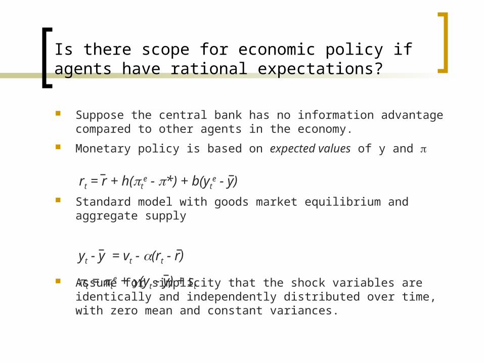
Suppose the central bank has no information advantage compared to other agents in the economy.

Monetary policy is based on expected values of y and

Standard model with goods market equilibrium and aggregate supply

Assume for simplicity that the shock variables are identically and independently distributed over time, with zero mean and constant variances.

yt - y = vt - (rt - r)

rt = r + h(te - *) + b(yt

e - y)

t = te + (yt - y) + st

Solving a model with rational expectations

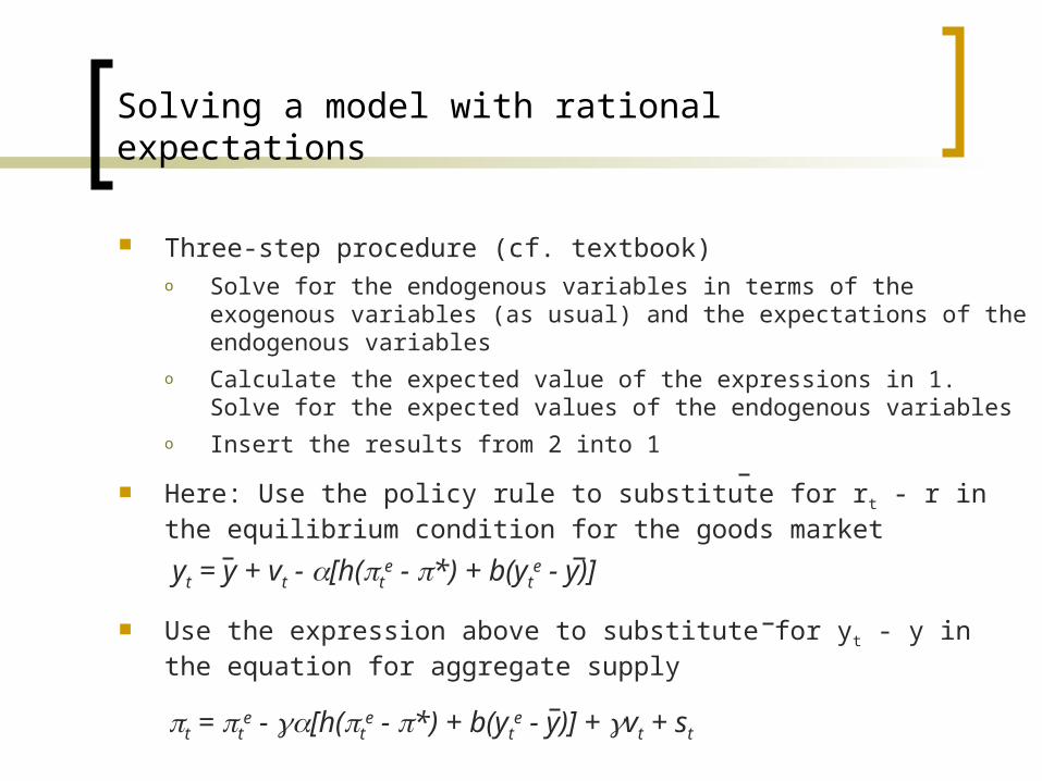
Three-step procedure (cf. textbook)o Solve for the endogenous variables in terms of the exogenous

variables (as usual) and the expectations of the endogenous variables

o Calculate the expected value of the expressions in 1. Solve for the expected values of the endogenous variables

o Insert the results from 2 into 1

Here: Use the policy rule to substitute for rt - r in the equilibrium condition for the goods market

Use the expression above to substitute for yt - y in the equation for aggregate supply

yt = y + vt - [h(te - *) + b(yt

e - y)]

t = te - [h(t

e - *) + b(yte - y)] + vt + st

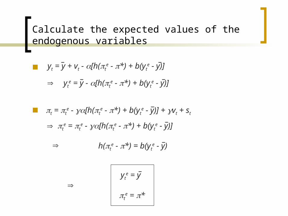
Calculate the expected values of the endogenous variables

yt = y + vt - [h(te - *) + b(yt

e - y)]

t = te - [h(t

e - *) + b(yte - y)] + vt + st

yte = y - [h(t

e - *) + b(yte - y)]

te = t

e - [h(te - *) + b(yt

e - y)]

h(te - *) = b(yt

e - y)

yte = y

te = *

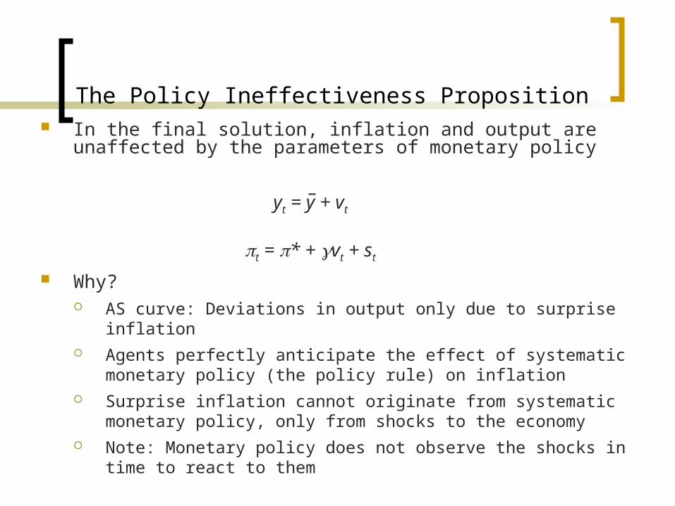
The Policy Ineffectiveness Proposition In the final solution, inflation and output are unaffected by the

parameters of monetary policy

Why? AS curve: Deviations in output only due to surprise inflation Agents perfectly anticipate the effect of systematic monetary policy

(the policy rule) on inflation Surprise inflation cannot originate from systematic monetary policy,

only from shocks to the economy Note: Monetary policy does not observe the shocks in time to react to

them

yt = y + vt

t = * + vt + st

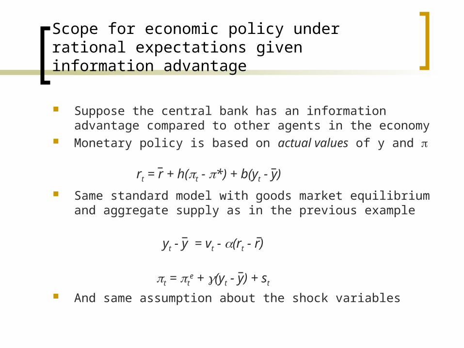
Scope for economic policy under rational expectations given information advantage

Suppose the central bank has an information advantage compared to other agents in the economy

Monetary policy is based on actual values of y and

Same standard model with goods market equilibrium and aggregate supply as in the previous example

And same assumption about the shock variables

yt - y = vt - (rt - r)

rt = r + h(t - *) + b(yt - y)

t = te + (yt - y) + st

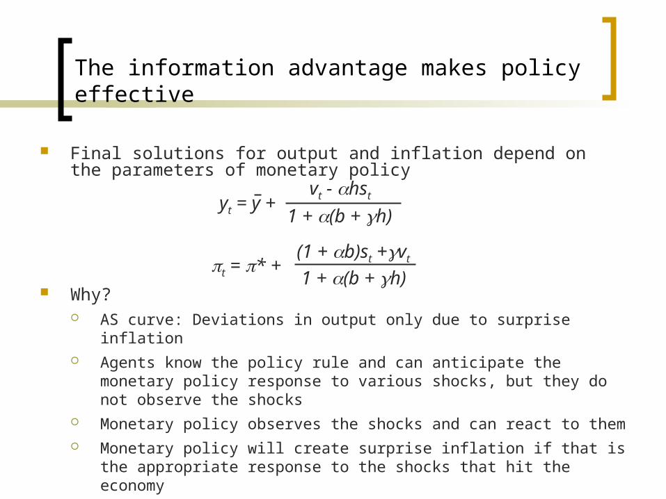
The information advantage makes policy effective

Final solutions for output and inflation depend on the parameters of monetary policy

Why? AS curve: Deviations in output only due to surprise inflation Agents know the policy rule and can anticipate the monetary policy

response to various shocks, but they do not observe the shocks Monetary policy observes the shocks and can react to them Monetary policy will create surprise inflation if that is the appropriate

response to the shocks that hit the economy

yt = y +1 + (b + h)

vt - hst

t = * + (1 + b)st +vt

1 + (b + h)

Ricardian equivalence: Ineffectiveness of tax policy

Related to the ideas behind the Policy Ineffectiveness Proposition is the Ricardian Equivalence Theorem (sect. 16.3)

Consumers have rational (forward-looking) expectations about taxes: They realize that a government tax cut today will necessitate a

tax increase in the future (through the intertemporal government budget constraint given no changes in government expenditure)

Consumers experience increased income through the tax cut, but they decide to save it in order to pay the increased taxes in the future

Conclusion: No effect on today’s consumption from a tax cut

The Lucas’ critique: Be cautious about historical econometric relationships

The Lucas’ critique is about the stability of econometric relationships: After a policy change, historical econometric relationships may no longer be valid because economic agents change their behavior

Implication for policy makers: Past behavior of economic agents can be a poor guide for assessing the effects of policy changes

Lucas: Should estimate parameters that are invariant to changes in government policy rules (so-called “deep” parameters) such as tastes or technology

PART 2

Real business cycles

Overview of real business cycles theory

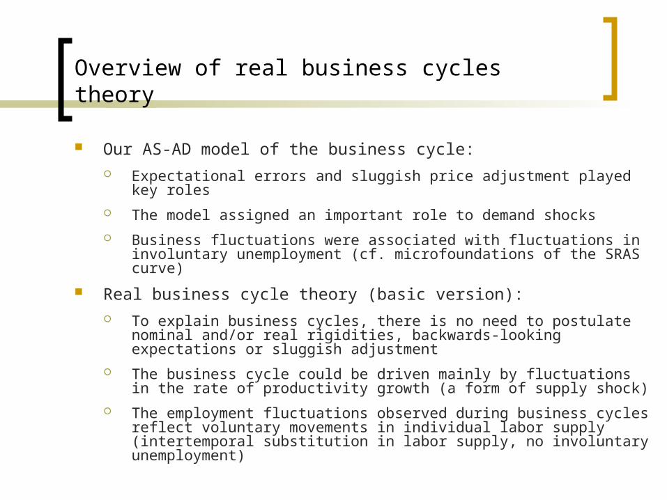
Our AS-AD model of the business cycle: Expectational errors and sluggish price adjustment played key roles

The model assigned an important role to demand shocks

Business fluctuations were associated with fluctuations in involuntary unemployment (cf. microfoundations of the SRAS curve)

Real business cycle theory (basic version): To explain business cycles, there is no need to postulate nominal

and/or real rigidities, backwards-looking expectations or sluggish adjustment

The business cycle could be driven mainly by fluctuations in the rate of productivity growth (a form of supply shock)

The employment fluctuations observed during business cycles reflect voluntary movements in individual labor supply (intertemporal substitution in labor supply, no involuntary unemployment)

In the simple RBC model, the production-side resembles a basic growth model

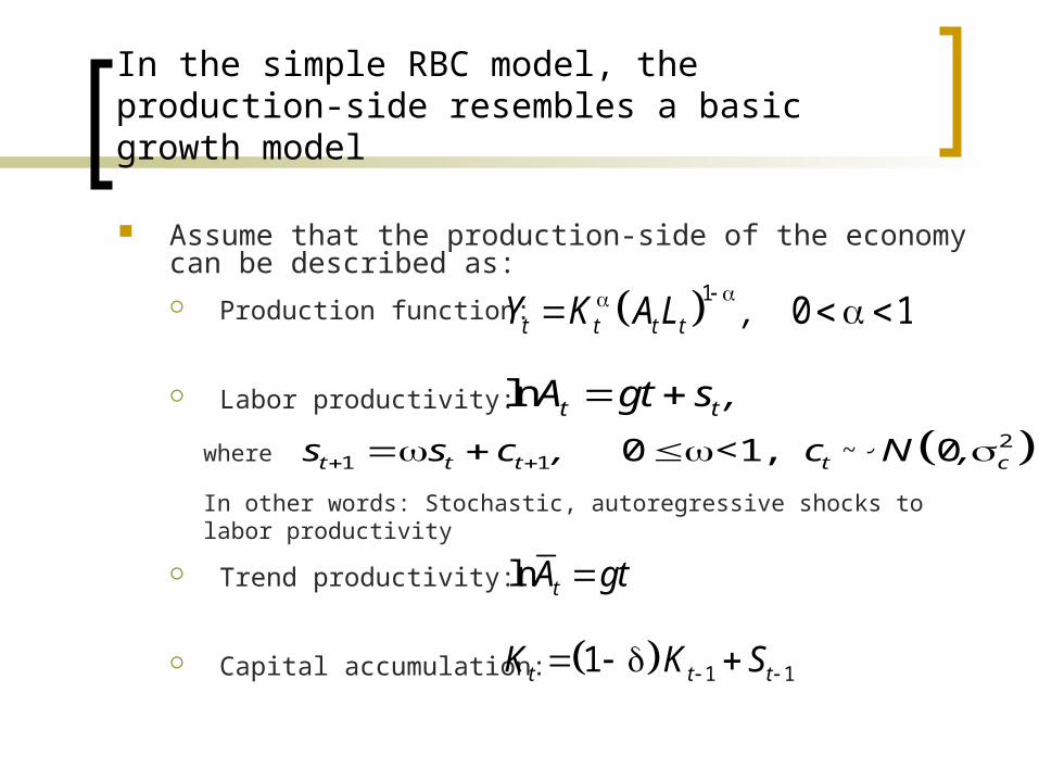
Assume that the production-side of the economy can be described as: Production function:

Labor productivity:

Trend productivity:

Capital accumulation:

1Production function: 0 1t t t tY K AL ,

21 1

Actual productivity: ln

0 <1, 0

t t

t t t t c

A gt s ,

s s c , c N ,

Trend productivity: ln tA gt

1 1Capital accumulation: 1t t tK K S

21 1

Actual productivity: ln

0 <1, 0

t t

t t t t c

A gt s ,

s s c , c N ,

where ~

In other words: Stochastic, autoregressive shocks to labor productivity

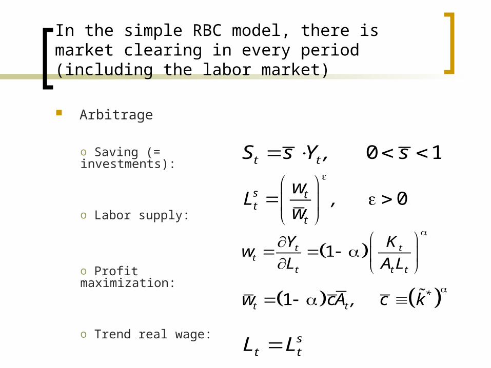
In the simple RBC model, there is market clearing in every period (including the labor market)

Arbitrage

Labour supply: 0s tt

t

wL ,

w

Saving: 0 1t tS s Y , s

Profit maximization: 1t tt

t t t

Y Kw

L AL

Trend real wage: 1 *t tw cA , c k

Labour market clearing: st tL L

o Saving (= investments):

o Labor supply:

o Profit maximization:

o Trend real wage:

o Labor market clearing:

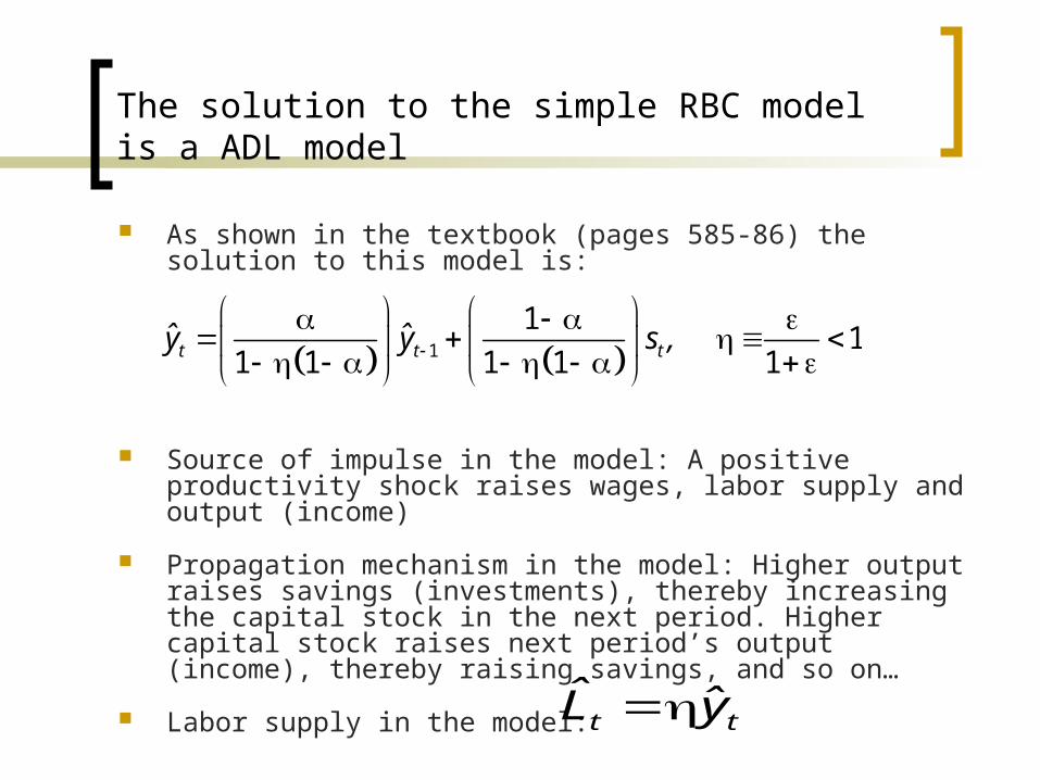
The solution to the simple RBC model is a ADL model

As shown in the textbook (pages 585-86) the solution to this model is:

Source of impulse in the model: A positive productivity shock raises wages, labor supply and output (income)

Propagation mechanism in the model: Higher output raises savings (investments), thereby increasing the capital stock in the next period. Higher capital stock raises next period’s output (income), thereby raising savings, and so on…

Labor supply in the model:

1

1 1

1 1 1 1 1t t tˆ ˆy y s ,

t tˆ ˆL y

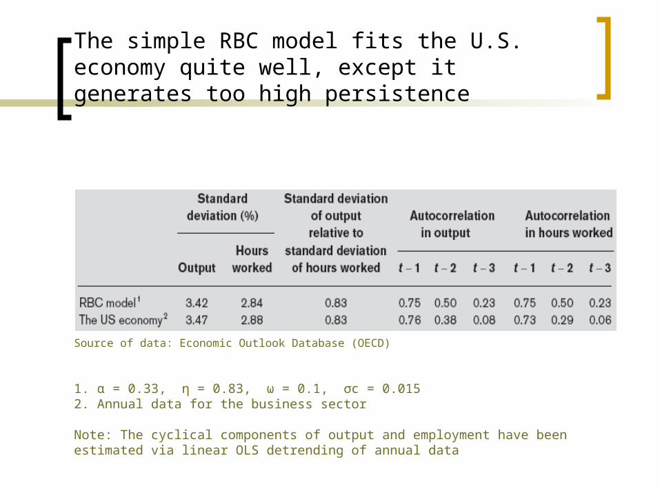
The simple RBC model fits the U.S. economy quite well, except it generates too high persistence

Source of data: Economic Outlook Database (OECD)

1. α = 0.33, η = 0.83, ω = 0.1, σc = 0.0152. Annual data for the business sector

Note: The cyclical components of output and employment have been estimated via linear OLS detrending of annual data

Some problems with the basic RBC theory

Is technological progress really so time-varying as postulated in the RBC model?

Is it really plausible that recessions are periods of technological regress?

Do the observed fluctuations in employment really reflect intertemporal substitution in labor supply? More generally: Is all recorded unemployment really voluntary?

The RBC model predicts that the real wage is procyclical. This is in line with U.S. data, but not consistent with European data.

Response: Real business cycle theorists have tried to make their models more realistic by allowing for various frictions and rigidities, including (in some cases) nominal rigidities.

The most influential contribution of real business cycle theory is methodological

At the methodological level, RBC theorists have made a lasting contribution by pointing out that: Supply shocks may play an important part in the explanation of

business cycles

A satisfactory theory of the business cycle should consist of a dynamic stochastic general equilibrium model which is able to reproduce the most important stylized facts of the business cycle

The Nobel committee on Kydland and Prescott’s business cycle models: “The Laureates laid the groundwork for more robust models by

regarding business cycles as the collective outcome of countless forward-looking decisions made by individual households and firms regarding consumption, investments, labor supply, etc. Kydland and Prescott's methods have been widely adopted in modern macroeconomics.”

PART 3

Rules versus discretion

Policy rules versus discretion: a credibility problem

Discretionary policy: Policy makers react in an ad-hoc manner to the specific circumstances of the situation, using all relevant available information

Intuitive advantage of discretionary policy: Flexibility to adopt the optimal policy at all times

Seminal article: Kydland and Prescott (1977) “Rules rather than discretion: The inconsistency of optimal plans”

Conclusion: Under plausible conditions, the government may achieve better results by committing to follow a rule for monetary policy

Provides a rationale for explicit inflation targets

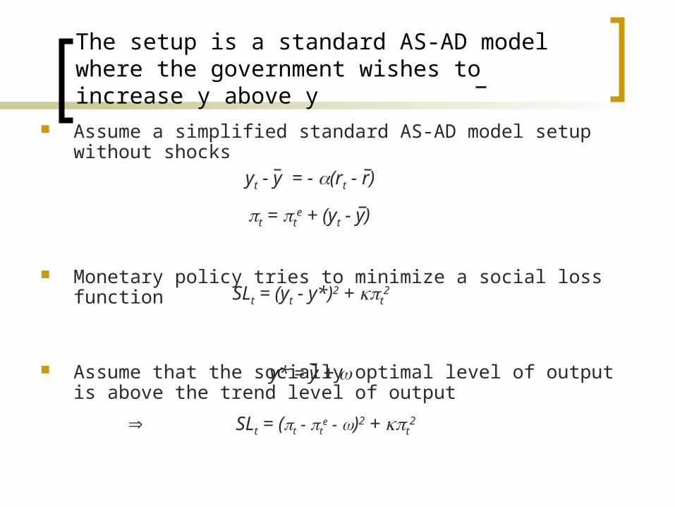
The setup is a standard AS-AD model where the government wishes to increase y above y

Assume a simplified standard AS-AD model setup without shocks

Monetary policy tries to minimize a social loss function

Assume that the socially optimal level of output is above the trend level of output

yt - y = - (rt - r)

t = te + (yt - y)

SLt = (yt - y*)2 + t2

y* = y +

SLt = (t - te - )2 + t

2

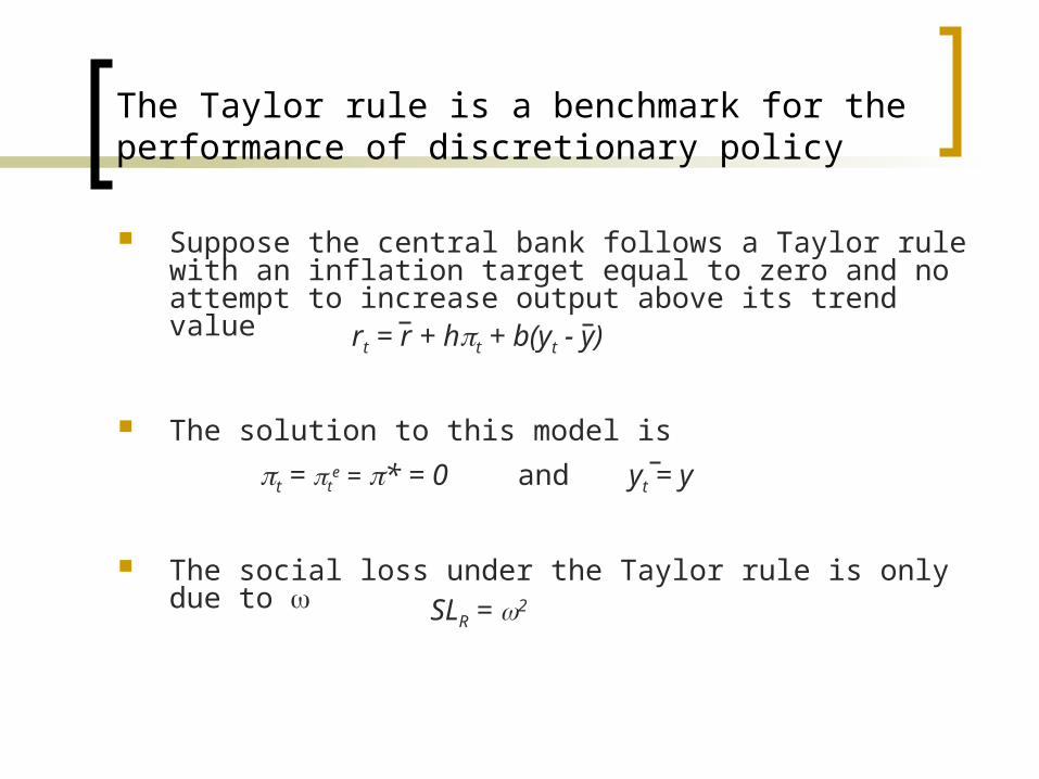
The Taylor rule is a benchmark for the performance of discretionary policy

Suppose the central bank follows a Taylor rule with an inflation target equal to zero and no attempt to increase output above its trend value

The solution to this model is

The social loss under the Taylor rule is only due to

rt = r + ht + b(yt - y)

SLR = 2

t = te = * = 0 and yt = y

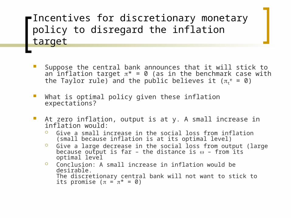
Incentives for discretionary monetary policy to disregard the inflation target

Suppose the central bank announces that it will stick to an inflation target * = 0 (as in the benchmark case with the Taylor rule) and the public believes it (t

e = 0)

What is optimal policy given these inflation expectations?

At zero inflation, output is at y. A small increase in inflation would: Give a small increase in the social loss from inflation (small

because inflation is at its optimal level) Give a large decrease in the social loss from output (large

because output is far – the distance is – from its optimal level Conclusion: A small increase in inflation would be desirable.

The discretionary central bank will not want to stick to its promise ( = * = 0)

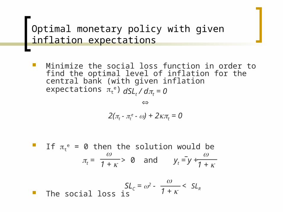
Optimal monetary policy with given inflation expectations

Minimize the social loss function in order to find the optimal level of inflation for the central bank (with given inflation expectations t

e)

If te = 0 then the solution would be

The social loss is

dSLt / dt = 0

2(t - te - ) + 2t = 0

t = > 01 +

and yt = y +1 +

SLC = 2 - < SLR1 +

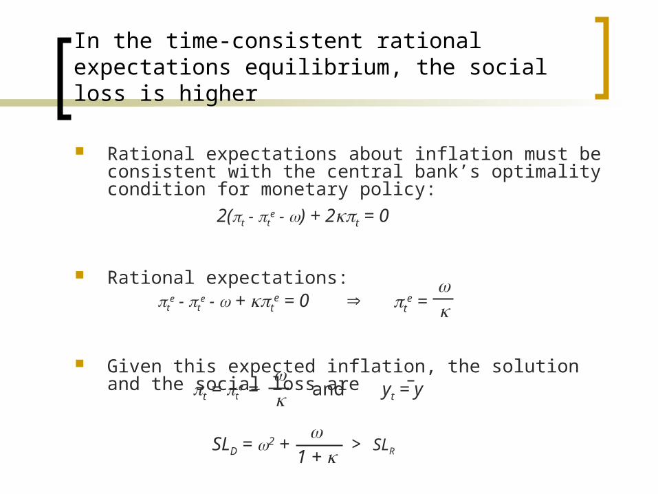
In the time-consistent rational expectations equilibrium, the social loss is higher

Rational expectations about inflation must be consistent with the central bank’s optimality condition for monetary policy:

Rational expectations:

Given this expected inflation, the solution and the social loss are

2(t - te - ) + 2t = 0

te - t

e - + te = 0 t

e =

SLD = 2 + > SLR1 +

t = te = and yt = y

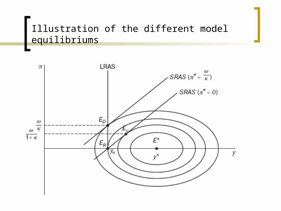
Illustration of the different model equilibriums

Central bank independence coupled with rules and/or reputation cures the inflation bias

Delegating monetary policy to the central bank keeps it at a distance from political incentives Instrument independence is common (operational indep.) Goal independence is more rare

Building reputation Repeated games: If the central bank can only brake its promise

once, the incentive to stick to the inflation target is increased Choose a “hawkish” central bank governor (tough on inflation)