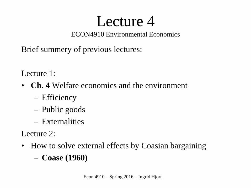
Lecture 4 ECON4910 Environmental Economics

Brief summery of previous lectures:

Lecture 1:

• Ch. 4 Welfare economics and the environment

– Efficiency

– Public goods

– Externalities

Lecture 2:

• How to solve external effects by Coasian bargaining

– Coase (1960)

Econ 4910 – Spring 2016 – Ingrid Hjort

Lecture 3 and 4:

• Ch. 5 Pollution targets

«How do we decide the optimal level of pollution?»

• Ch. 6 Pollution instruments

«How can we achieve these targets?»

– Montgomery (1975): Market in licenses

– Bård’s blackboard-model: Tax and double dividend

CHAPTER 5

Pollution control: targets

The Damage function:

The Benefit function:

Where M is aggregate emission flow

of all emission sources:

• Total damage is thought to rise at an increasing rate, with the size

of the emission flow. The more emissions thus more harm on

nature. Convex

• Total benefits will rise at a decreasing rate as more emissions are

used in production, assuming decreasing marginal productivity.

Concave

( )D D M

( )B B M

1

n

i

i

M m

What is the efficient level of pollution?

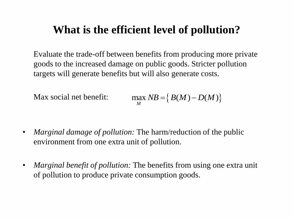
What is the efficient level of pollution?

Evaluate the trade-off between benefits from producing more private

goods to the increased damage on public goods. Stricter pollution

targets will generate benefits but will also generate costs.

Max social net benefit:

• Marginal damage of pollution: The harm/reduction of the public

environment from one extra unit of pollution.

• Marginal benefit of pollution: The benefits from using one extra unit

of pollution to produce private consumption goods.

max ( ) ( )M

NB B M D M

'( )B M

Maximised net

benefits

M*

*

Emissions, M

D(M)

B(M)

Emissions, M

Figure 5.2 Total and marginal damage and benefit functions, and the efficient level of flow pollution emissions

'( )D M

M̂

B

A

( )D M

( )B M

Comment to figure 5.2

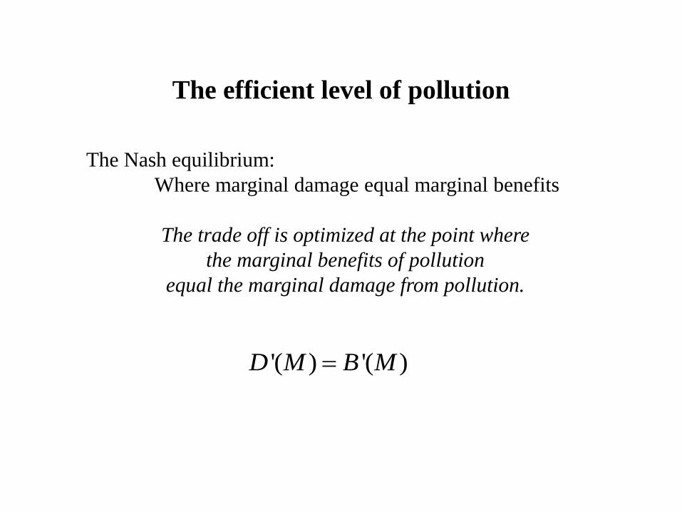
The efficient level of pollution

'( ) '( )D M B M

The Nash equilibrium:

Where marginal damage equal marginal benefits

The trade off is optimized at the point where

the marginal benefits of pollution

equal the marginal damage from pollution.

There exist different types of pollution problems I

1. Flow-damage pollution: the damage depend

on the rate of the emission flow alone. That is, the

instant rate at which they are being discharged into the

environmental system.

2. Stock-damage pollution: damages depend only

on the stock of pollution in the relevant environmental

system at any point in time. Stock pollutants accumulate

in the environment over time. Stock pollutants are

persistent over time, and may be transported over space,

two dimensional.

Pollution flows and pollution stocks

• The static flow pollution model: (noise, light, smell, smoke)

These problems have no time dimension, the pollution

stops when the emissions stops. Flow-damage pollution: D = D(M) (5.1a)

• The stock pollution problem:

Emissions (M) accumulate and create a stock (A) of a

harmful substance. Stock-damage pollution: D = D(A) (5.1b)

Stock pollutants can create a burden for future generations by passing on damage

that persists well after the benefits received from incurring that damage have been

forgotten.

The distinction between flows and stocks becomes crucial for

two reasons

First,

This distinction enables us to understand the science lying behind the

pollution problem and translate this into economic models.

Second,

The distinction is important for policy purposes.

While the damage is associated with the pollution stock, that stock is outside

the direct control of policy makers. Environmental protection agencies may,

however, be able to control the rate of emission flows. Even where they

cannot control such flows directly, the regulator may find it more convenient

to target emissions rather than stocks. Given that what we seek to achieve

depends on stocks but what is controlled or regulated are typically flows, it is

necessary to understand the linkage between the two.

There exist different types of pollution problems II

3. Uniformly mixing: the damage depends upon the total

amount of the pollutant entering the system, independent of

geographical location, e.g., green house gases

4. Non-uniformly mixing: the damage is relatively sensitive

to where emissions are injected into the environmental system. The

concentration rate of the pollutant vary from place to place

Uniformly mixing

• By definition, the location of the uniformly mixing (UM) emission

source is irrelevant

– All that matters, as far as concentration rates at any receptor are concerned, is the

total amount of those emissions.

• Mixing of a pollutant refers to the extent to which physical processes

cause the pollutant to be dispersed or spread out.

• A pollutant is uniformly mixing if the pollutant quickly becomes

dispersed to the point where its spatial distribution is uniform.

– That is, the measured concentration rate of the pollutant does not vary from place

to place.

– This property is satisfied, for example, by most greenhouse gases.

• Policy: Focus on minimizing the total pollution level, finding the cost

effective allocation of responsibility.

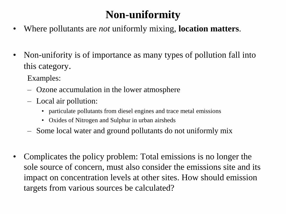
Non-uniformity

• Where pollutants are not uniformly mixing, location matters.

• Non-unifority is of importance as many types of pollution fall into

this category.

Examples:

– Ozone accumulation in the lower atmosphere

– Local air pollution:

• particulate pollutants from diesel engines and trace metal emissions

• Oxides of Nitrogen and Sulphur in urban airsheds

– Some local water and ground pollutants do not uniformly mix

• Complicates the policy problem: Total emissions is no longer the

sole source of concern, must also consider the emissions site and its

impact on concentration levels at other sites. How should emission

targets from various sources be calculated?

CHAPTER 6

Pollution control:

instruments

The target: the emission target should be set such that the

aggregate marginal benefit from emissions equals the

aggregate marginal damage

MB MD

The target

The instrument: should be cost-efficient.

– The cost of achieving a given reduction in emissions will be

minimized if and only if the marginal costs of emission reduction

are equalized for all emitters

The instrument

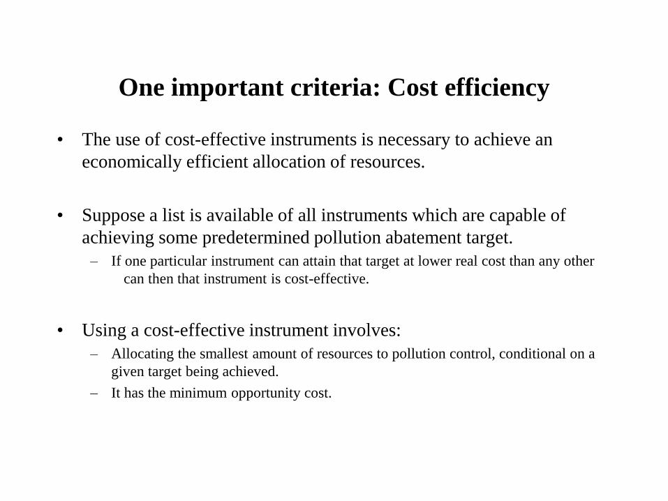
One important criteria: Cost efficiency

• The use of cost-effective instruments is necessary to achieve an

economically efficient allocation of resources.

• Suppose a list is available of all instruments which are capable of

achieving some predetermined pollution abatement target.

– If one particular instrument can attain that target at lower real cost than any other

can then that instrument is cost-effective.

• Using a cost-effective instrument involves:

– Allocating the smallest amount of resources to pollution control, conditional on a

given target being achieved.

– It has the minimum opportunity cost.

Least-cost theorem

The least cost theorem: A necessary condition to achieve abatement at

least cost. The marginal cost of abatement is equalized over all polluting

firms (equimarginal principle)

– Abatement: Emission reduction

• Focus on abatement effort: polluters that can abate at least cost.

• This result is known as the least-cost theorem of pollution control.

• Illustrated in next figure

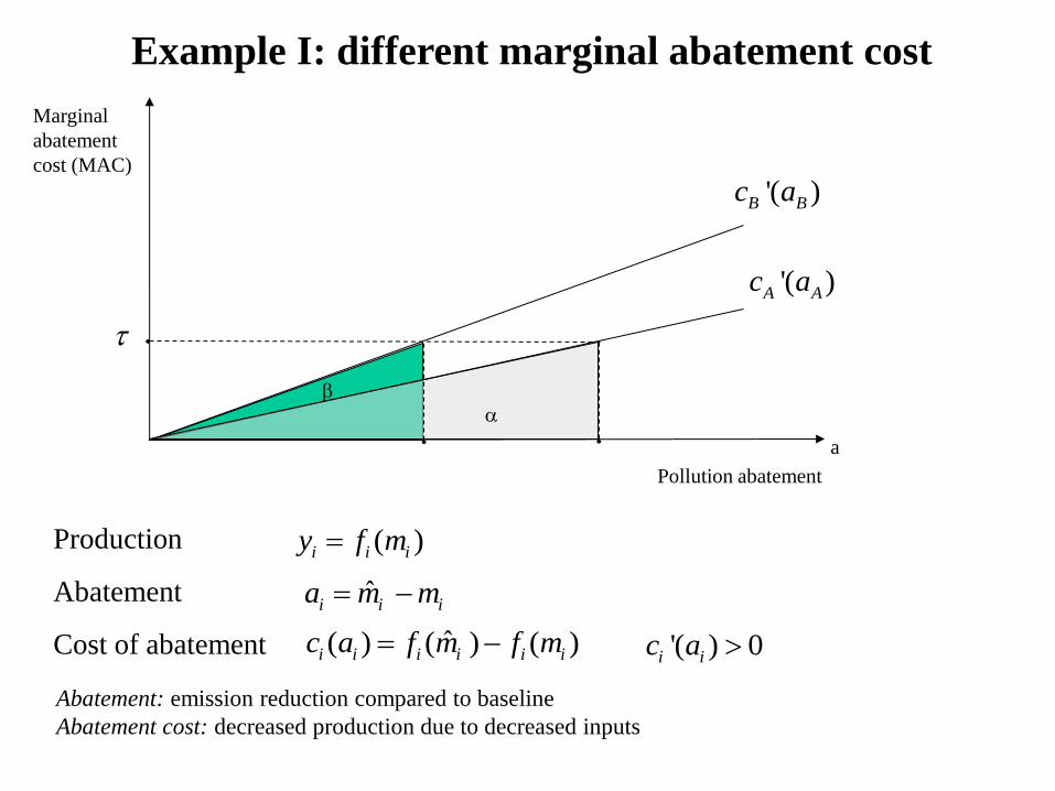
Pollution abatement

a

Marginal

abatement

cost (MAC)

Example I: different marginal abatement cost

( )i i iy f m

ˆ( ) ( ) ( )i i i i i ic a f m f m

ˆi i ia m m

Production

Abatement

Cost of abatement

Abatement: emission reduction compared to baseline

Abatement cost: decreased production due to decreased inputs

'( ) 0i ic a

'( )A Ac a

'( )B Bc a

The social planner will

minimize total abatement cost

for all firms, given the target

Example II: equal marginal abatement cost

1

min ( ) . *i

k

im

i

c a s t M M

ˆ( ) ( ) ( )i i i i i ic a f m f m

1

k

j

i

m M

1 1

ˆ( ) ( ) *k k

i i i

i i

f m f m m M

Show that the least cost theorem holds,

i.e., the shadow price of emission

reduction equals across firms

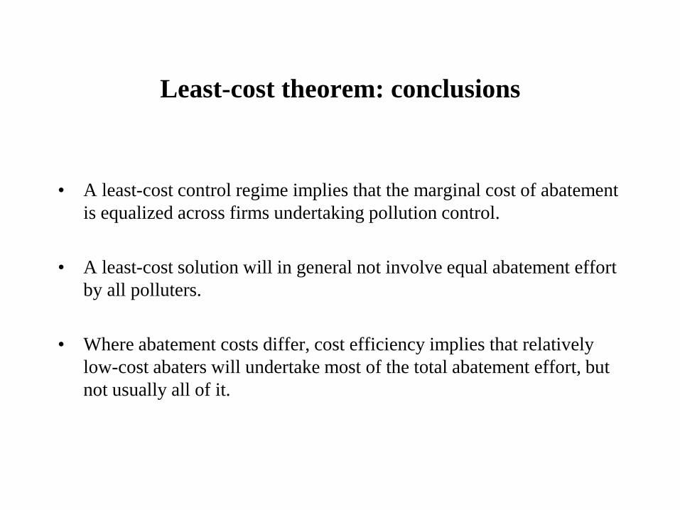
Least-cost theorem: conclusions

• A least-cost control regime implies that the marginal cost of abatement

is equalized across firms undertaking pollution control.

• A least-cost solution will in general not involve equal abatement effort

by all polluters.

• Where abatement costs differ, cost efficiency implies that relatively

low-cost abaters will undertake most of the total abatement effort, but

not usually all of it.

Instruments

for achieving pollution abatement targets

1) Voluntary approaches

2) Command and control

3) Economic incentive based instruments

1) Voluntary approaches

Bargaining solutions

• In a classic paper, Ronald Coase (1960) explored the connection between

property rights and the likelihood of efficient bargaining solutions to

inefficient allocations of resources.

– well defined and enforceable allocation of property rights.

– No transactions costs.

• Bargaining may lead to some abatement as every consumer is willing to pay

up something to avoid emissions...

...but not enough to reach the social optimum, since the environment is

a public good, causing free-rider problems

Liability

• The judicial system may help to bring about efficient outcomes

– An implicit assumption in the discussion of bargaining, enforcement of the contract

• Liability can be used to deal with environmental hazards, by incentivize the

efficient level of precautionary behavior

• Suppose: a general legal principle is established, making agents liable for the

adverse external effects of their actions

The challenges with climate change

• The absence of supra-national sovereign institutions makes it difficult to

legally enforce the Coasian-bargaining solutions (global climate treaties)

• Compensation: How can we determine whose emissions are causing what

damages

• Use of liability face a difficulty where damage appear long time after the

relevant pollutants were discharged (such as climate change). How to track

down those who are liable? Those responsible – individuals or firms – may no

longer exist…

– Related to this is a wider class of pollution problems in which actions undertaken in earlier

times, often over decades or even centuries, leave a legacy of polluted water, land, or biological

resources.

– Even if one could identify the polluting culprits and apportion blame appropriately, it is not

clear whether an ex post liability should be imposed.

2) Command and control instruments

• The dominant method of reducing pollution in most countries has been the

use of direct controls over polluters.

– This set of controls is commonly known as command and control instruments.

• Examples: prohibitions, restrictions, production standards

Attractive Properties

• Certainty of outcome

• Ability to get desired results very quickly.

Unattractive Properties

• Likely to be cost-inefficient, contain no mechanisms to bring about:

– equalization of marginal abatement costs over the controlled firms in that programme.

– equalization of marginal abatement costs across different programmes

• Lack good dynamic incentives

Each firm maximize profit given

the «command and control»-cap

imposed by the government:

Example: Command and control policy

max ( ) . .i

i i i i im

f m K s t m m

( ) ( )i i i i if m K m m

The shadow price is no longer

equal for all firms, this instrument

is not cost effective.

Firms differ in technology, but faces the same cap

If the government has all information about each firm’s marginal

abatement cost function, an individual cap can be imposed on all

firms. This would be a cost effective instrument. (Is this feasible?)

'( )i i if m

Command and control

• Required technology controls sometimes blur the pollution target/pollution instrument

distinction we have been using.

• The target actually achieved tends to emerge jointly with the administration of the

instrument.

• Sometimes government sets a general target (such as the reduction of particulates from

diesel engines by 25% over the next 5 years) and then pursues that target using a variety

of instruments applied at varying rates of intensity over time.

• Although technology-based instruments may be lacking in cost-effectiveness terms, they

can be very powerful; they are sometimes capable of achieving large reductions in

emissions quickly, particularly when technological ‘fixes’ are available but not widely

adopted.

• Technology controls have almost certainly resulted in huge reductions in pollution

levels compared with what would be expected in their absence.

• Incentive-based instruments work by altering the structure of pay-offs that

agents face, thereby creating incentives for individuals or firms to voluntarily

change their behavior.

• The pay-off structures are altered by changing relative prices.

• This can be done in many ways.

1. By the imposition of taxes on polluting emissions (or on outputs or activities deemed to be

environmentally harmful)

2. By the payment of subsidies for emissions abatement (or reduction of outputs or activities

deemed to be environmentally harmful)

3. By the use of tradable emission permit systems in which permits command a market price.

Those prices are, in effect, the cost of emitting pollutants

• More generally, any instrument which manipulates the price system in such a

way as to alter relative prices could also be regarded as an incentive-based

instrument.

3) Economic incentive instruments

• Emission quota:

p is the price of quotas

• Tax on emissions

• Quotas and taxes equalize if

• Subsidize abatement

• Taxes and subsidies are equivalent if

Example: Economic incentive instrument

max ( ) ( )i

i i i i im

f m K p m m

ˆmax ( ) ( )i

i i i i im

f m K s m m

max ( )i

i i i i im

f m K m

p

s

An economically efficient emissions tax

a abatement, a

Marginal benefit

of emissions

emissions, M

Marginal damage

Marginal cost of

abatement

Marginal benefit of

abatement

The economically efficient level of emissions abatement

'( )D M

BAUM*M

*

B'( )M

(before tax)

(after tax)

*

* *BAUa M M

'( )c a

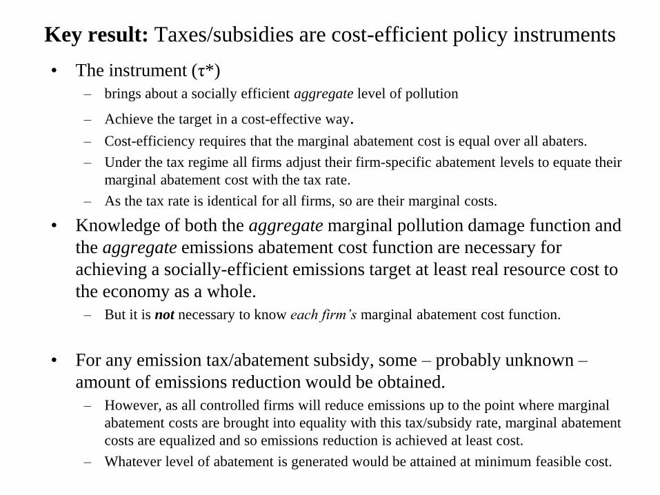
Key result: Taxes/subsidies are cost-efficient policy instruments

• The instrument (τ*)

– brings about a socially efficient aggregate level of pollution

– Achieve the target in a cost-effective way.

– Cost-efficiency requires that the marginal abatement cost is equal over all abaters.

– Under the tax regime all firms adjust their firm-specific abatement levels to equate their

marginal abatement cost with the tax rate.

– As the tax rate is identical for all firms, so are their marginal costs.

• Knowledge of both the aggregate marginal pollution damage function and

the aggregate emissions abatement cost function are necessary for

achieving a socially-efficient emissions target at least real resource cost to

the economy as a whole.

– But it is not necessary to know each firm’s marginal abatement cost function.

• For any emission tax/abatement subsidy, some – probably unknown –

amount of emissions reduction would be obtained.

– However, as all controlled firms will reduce emissions up to the point where marginal

abatement costs are brought into equality with this tax/subsidy rate, marginal abatement

costs are equalized and so emissions reduction is achieved at least cost.

– Whatever level of abatement is generated would be attained at minimum feasible cost.

Tradable emissions permits

• Marketable permit systems are based on the principle than any increase in

emissions must be offset by an equivalent decrease elsewhere.

• There is a limit on the total quantity of emissions allowed

• The regulator does not attempt to determine how quotas are allocated

among firms, because they trade until the equilibrium is met.

• However, initial allocation must be determined

• Allocate the quotas for free = subsidizing

• Firms have to bargain over quotas: may give distributional effects

All the way, through out this lecture, we have implicitly

assumed perfect information and full understanding of the

damages and benefits from pollution.

What about policy regulations under

imperfect information?

Readings to next lecture:

Weitzman (1974) Prices vs. Quantities

Appendix and further reading to

lecture 4

Efficient flow-damage pollution Pollution damage depends directly on the level of emissions

5.5 A static model of efficient flow pollution

• Emissions have both benefits and costs.

• We call the costs of emissions ‘damages’.

• These damages can be thought of as a negative (adverse) externality.

• For simplicity, we suppose that damage is independent of the time and the

source of the emissions, and that emissions have no effect outside the economy

being studied. We relax these assumptions later.

• An efficient level of emissions is one that maximises the net benefits from

pollution, where net benefits are defined as pollution benefits minus pollution

damages.

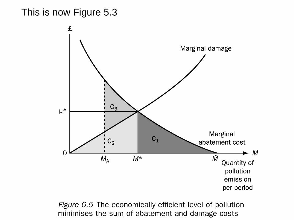
This is now Figure 5.3

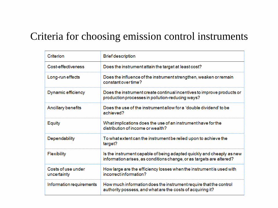
Criteria for choosing emission control instruments

Instrument category

Institutional approaches to

facilitate internalisation of

externalities

Command and control

instruments

Economic incentive (market-

based) instruments

Table 6.2 Classification of pollution control instruments

Instrument category Description

Institutional approaches to

facilitate internalisation of

externalities

Facilitation of bargaining Cost of, or impediments to, bargaining are

reduced

Specification of liability Codification of liability for environmental

damage

Development of social responsibility Education and socialisation programmes

promoting ‘citizenship’

Instrument category Description

Command and control

instruments

Input controls over quantity and/or mix of

inputs

Requirements to use particular inputs, or

prohibitions/restrictions on use of others

Technology controls Requirements to use particular methods or

standards

Output quotas or prohibitions Non-transferable ceilings on product

outputs

Emissions licences Non-transferable ceilings on emission

quantities

Location controls (zoning, planning

controls, relocation)

Regulations relating to admissible location

of activities

Instrument category Description

Economic incentive (market-

based) instruments

Emissions charges/taxes Direct charges based on quantity and/or

quality of a pollutant

User charges/fees/natural resource taxes Payment for cost of collective services

(charges), or for use of a natural resource

(fees or resource taxes)

Product charges/taxes Applied to polluting products

Emissions abatement and resource

management subsidies

Financial payments designed to reduce

damaging emissions or conserve scarce

resources

Marketable (transferable, marketable)

emissions permits

Two systems: those based on emissions

reduction credits (ERCs) or cap-and-trade

Deposit-refund systems A fully or partially reimbursable payment

incurred at purchase of a product

Non-compliance fees Payments made by polluters or resource

users for non-compliance, usually

proportional to damage or to profit gains

Performance bonds A deposit paid, repayable on achieving

compliance

Liability payments Payments in compensation for damage

• The target: the emission target should be set such that the

aggregate marginal benefit from emissions equals the

aggregate marginal damage

• The efficient level of emissions: the marginal abatement

cost should equal the total willingness to pay for a

marginal improvement of environmental policy

MB MD

MAC WTP

0

( , )

'( ) '( ) 0

'( )

'( )

( )

( )

'( )

( )

'( )'( ) '( )

'( )

'( ) ( )

'( )'( ) '( )

'( )

i

i i

i

i

i i

i

i

U u y E

u y dy u E dE

u Edy dE

u y

z m

E E z m

dEz m

dm

y f m

u Ef m z m

u y

B M f m

u ED M z m

u y

How much are

consumers

willing to pay

for a marginal

improvement

in the public

good of

environment?

Preferences

Total derivative

How much you are willing to give up of

the private good to achieve a marginal

improvement of the public good

Some damage function

Environmental quality

Firm’s production

Marginal benefits from emissions

Marginal damage from emissions