Learning Occupancy Grid Maps With Forward Sensor Models

Sebastian Thrun

School of Computer Science

Carnegie Mellon University

Pittsburgh, PA 15213

Abstract

This article describes a new algorithm for acquiring occupancy grid maps with mobile

robots. Existing occupancy grid mapping algorithms decompose the high-dimensional map-

ping problem into a collection of one-dimensional problems, where the occupancy of each

grid cell is estimated independently. This induces conflicts that may lead to inconsistent

maps, even for noise-free sensors. This article shows how to solve the mapping problem in

the original, high-dimensional space, thereby maintaining all dependencies between neigh-

boring cells. As a result, maps generated by our approach are often more accurate than those

generated using traditional techniques. Our approach relies on a statistical formulation of

the mapping problem using forward models. It employs the expectation maximization algo-

rithm for searching maps that maximize the likelihood of the sensor measurements.

1 Introduction

In the past two decades, occupancy grid maps have become a dominant paradigm for envi-

ronment modeling in mobile robotics. Occupancy grid maps are spatial representations of robot

environments. They represent environments by fine-grained, metric grids of variables that reflect

the occupancy of the environment. Once acquired, they enable various key functions necessary

for mobile robot navigation, such as localization, path planning, collision avoidance, and people

finding.

The basic occupancy grid map paradigm has been applied successfully in many different

ways. For example, some systems use maps locally, to plan collision-free paths or to identify

environment features for localization [1, 10, 19, 20]. Others, such as many of the systems de-

scribed in [11, 23], rely on global occupancy grid maps for global path planning and navigation.

1

S� S�S�

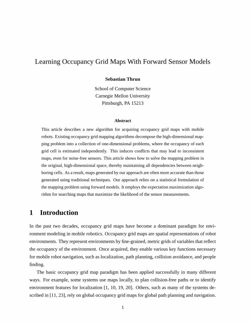
Figure 1: A set of noise-free sonar measurements that a robot may receive while passing an open door. While the

measurements are perfectly consistent, existing occupancy grid maps induce a conflict in the door region, where

short and long sensor cones overlap. This article presents a method that overcomes this problem.

Occupancy maps have been built using sonar sensors [15, 26], laser range finders [23], and stereo

vision [3, 16, 17]. While most existing occupancy mapping algorithms use two-dimensional

maps, some actually develop three-dimensional, volumetric maps [16]. Various authors have

investigated building such maps while simultaneously localizing the robot [4, 23, 27] and during

robot exploration [5, 21, 22, 26]. Some authors have extended occupancy grid maps to contain

enriched information, such as information pertaining to the reflective properties of the surface

materials [9]. Occupancy grid maps are arguably the most successful environment representa-

tion in mobile robotics to date [11].

Existing occupancy grid mapping algorithms suffer a key problem. They often generate

maps that are inconsistent with the data, particularly in cluttered environments. This problem is

due to the fact that existing algorithms decompose the high-dimensional mapping problem into

many one-dimensional estimation problems—one for each grid cell—which are then tackled

independently. The problem is common in environments like the one shown in Figure 1, where

a moving robot passes by an open door. Under conventional occupancy grid mapping algorithms,

the sonar measurements are conflicting with one another in the region of the doorway—which

often leads to the doorway being closed in the final map.

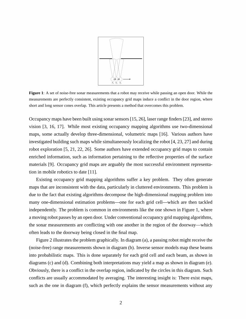
Figure 2 illustrates the problem graphically. In diagram (a), a passing robot might receive the

(noise-free) range measurements shown in diagram (b). Inverse sensor models map these beams

into probabilistic maps. This is done separately for each grid cell and each beam, as shown in

diagrams (c) and (d). Combining both interpretations may yield a map as shown in diagram (e).

Obviously, there is a conflict in the overlap region, indicated by the circles in this diagram. Such

conflicts are usually accommodated by averaging. The interesting insight is: There exist maps,

such as the one in diagram (f), which perfectly explains the sensor measurements without any

2

�� �� �

� ��

FRQIOLFW

��

(a) (b) (c)

(d) (e) (f)

Figure 2: The problem with current occupancy grid mapping algorithms: For the environment shown in Figure

(a), a passing robot might receive the (noise-free) measurement shown in (b). Inverse sensor models map these

beams into probabilistic maps. This is done separately for each grid cell and each beam, as shown in (c) and (d).

Combining both interpretations may yield a map as shown in (e). Obviously, there is a conflict in the overlap region,

indicated by the circles in (e). The interesting insight is: There exist maps, such as the one in diagram (f), which

perfectly explain the sensor measurement without any such conflict. For a sensor reading to be explained, it suffices

to assume an obstacle somewhere in the cone of a measurement, and not everywhere. This effect is captured by the

forward models described in this article.

such conflict. This is because for a sensor reading to be explained, it suffices to assume an obsta-

cle somewhere in its measurement cone. Put differently, the fact that cones sweep over multiple

grid cells induces important dependencies between neighboring grid cells. A decomposition of

the mapping problem into thousands of binary estimation problems—as is common practice in

the literature—does not consider these dependencies and therefore may yield suboptimal results.

While this consideration uses sonar sensors as motivating example, it is easily extended

to certain other sensor types that may be used for building occupancy maps, such as stereo

vision [17]; it is, however, less applicable to laser range finders, due to their relatively small

angular perceptual field. This article derives an alternative algorithm, which solves the mapping

3

problem in the original, high-dimensional space [24]. In particular, our approach formulates the

mapping problem as a maximum likelihood problem in a high-dimensional space, often with tens

of thousands of dimensions. The estimation is carried out using the expectation maximization

algorithm (in short: EM) [6], which is a popular statistical tool. A key feature of our approach

is that it relies on forward probabilistic models of sensors, which model the physics of sensors.

This is in contrast to the literature on occupancy grid mapping, which typically uses inverse

models for interpreting sensor measurements. To obtain a probabilistic map with uncertainty,

we calculate marginals of the occupancy probability of each grid cell conditioned on the map

found by EM. Empirical results show that our approach yields considerably more accurate maps.

2 Occupancy Grid Mapping with Inverse Models

This section establishes the basic mathematical notation and derives the basic occupancy grid

mapping approach [7, 14, 16]. Standard occupancy methods are characterized by two algorith-

mic choices:

1. They decompose the high-dimensional mapping problem into many binary estimation

problems, which are then solved independently of each other.

2. They rely on inverse models of the robot’s sensors which reasons from sensor measure-

ments to maps (opposite of the way sensor data is generated).

As discussed in the introduction to this article, this decomposition creates conflicts even for

noise-free data. Techniques such as Bayesian reasoning are then employed to resolve these

conflicts. We view this approach as computationally elegant but inferior to methods that treat

the mapping problem for what it is: A problem in a high dimensional space.

Let m be the occupancy grid map. We use mx,y to denote the occupancy of the grid cell with

index 〈x, y〉. Occupancy grid maps are estimated from sensor measurements (e.g., sonar mea-

surements). Let z1, . . . , zT denote the measurements from time 1 through time T , along with

the pose at which the measurement was taken (which is assumed to be known). For example, zt

might be a sonar scan and a three-dimensional pose variable (x-y coordinates of the robot and

heading direction). Each measurement carries information about the occupancy of many grid

cells. Thus, the problem addressed by occupancy grid mapping is the problem of determining

the probability of occupancy of each grid cell m given the measurements z1, . . . , zT :

p(m | z1, . . . , zT ) (1)

4

Maps are defined over high-dimensional spaces. Therefore, this posterior cannot be represented

easily. Standard occupancy grid mapping techniques decompose the problem into many one-

dimensional estimation problems, which are solved independently of each other. These one-

dimensional problems correspond to estimation problems for the individual cells mx,y of the

grid:

p(mx,y | z1, . . . , zT ) (2)

For computational reasons, it is common practice to calculate the so-called log-odds of p(mx,y |z1, . . . , zT ) instead of estimating the posterior p(mx,y | z1, . . . , zT ). The log-odds is defined as

follows:

lTx,y = logp(mx,y | z1, . . . , zT )

1 − p(mx,y | z1, . . . , zT )(3)

The log-odds can take on any value in <. From log-odds lTx,y defined in (3), it is easy to “recover”

the posterior occupancy probability p(mx,y | z1, . . . , zT ):

p(mx,y | z1, . . . , zT ) = 1 − [elTx,y ]−1 (4)

The log-odds at any point in time t is estimated recursively via Bayes rule, applied to the poste-

rior p(mx,y | z1, . . . , zt):

p(mx,y | z1, . . . , zt) =p(zt | z1, . . . , zt−1,mx,y) p(mx,y | z1, . . . , zt−1)

p(zt | z1, . . . , zt−1)(5)

A common assumption in mapping is the static world assumption, which states that past sensor

readings are conditionally independent given knowledge of the map m, for any point in time t:

p(zt | z1, . . . , zt−1,m) = p(zt | m) (6)

This assumption is valid in static environments with a non-changing map. It will also be made

by our approach. However, by virtue of the grid decomposition, occupancy grid maps make

a much stronger assumption: They assume conditional independence given knowledge of each

individual grid cell mx,y, regardless of the occupancy of neighboring cells:

p(zt | z1, . . . , zt−1,mx,y) = p(zt | mx,y) (7)

This is an incorrect assumption even in static worlds, since sensor measurements (e.g., sonar

cones) sweep over multiple grid cells, all of which have to be known for obtaining independence.

5

However, this conditional independence assumption is convenient. It allows us to simplify (5)

to:

p(mx,y | z1, . . . , zt) =p(zt | mx,y) p(mx,y | z1, . . . , zt−1)

p(zt | z1, . . . , zt−1)(8)

Applying Bayes rule to the term p(zt | mx,y) gives us:

p(mx,y | z1, . . . , zt) =p(mx,y | zt) p(zt) p(mx,y | z1, . . . , zt−1)

p(mx,y) p(zt | z1, . . . , zt−1)(9)

This equation computes the probability that mx,y is occupied.

A completely analogous derivation leads to the posterior probability that the grid cell mx,y

is free. Freeness will be denoted mx,y:

p(mx,y | z1, . . . , zt) =p(mx,y | zt) p(zt) p(mx,y | z1, . . . , zt−1)

p(mx,y) p(zt | z1, . . . , zt−1)(10)

By dividing (9) by (10), we can eliminate several hard-to-compute terms:

p(mx,y | z1, . . . , zt)

p(mx,y | z1, . . . , zt)=

p(mx,y | zt)

p(mx,y | zt)

p(mx,y)

p(mx,y)

p(mx,y | z1, . . . , zt−1)

p(mx,y | z1, . . . , zt−1)(11)

This expression is actually in the form of an odds ratio. To see, we notice that p(mx,y) =

1− p(mx,y), and p(mx,y | ·) = 1− p(mx,y | ·) for any conditioning variable “·”. In other words,

we can re-write (11) as follows:

p(mx,y | z1, . . . , zt)

1 − p(mx,y | z1, . . . , zt)=

p(mx,y | zt)

1 − p(mx,y | zt)

1 − p(mx,y)

p(mx,y)

p(mx,y | z1, . . . , zt−1)

1 − p(mx,y | z1, . . . , zt−1)(12)

The desired log-odds is the logarithm of this expression:

logp(mx,y | z1, . . . , zt)

1 − p(mx,y | z1, . . . , zt)

= logp(mx,y | zt)

1 − p(mx,y | zt)+ log

1 − p(mx,y)

p(mx,y)+ log

p(mx,y | z1, . . . , zt−1)

1 − p(mx,y | z1, . . . , zt−1)(13)

By substituting in the log-odds ltx,y as defined above, we arrive at the recursive equation:

ltx,y = logp(mx,y | zt)

1 − p(mx,y | zt)+ log

1 − p(mx,y)

p(mx,y)+ lt−1

x,y (14)

with the initialization

l0x,y = logp(mx,y)

p(1 − mx,y)(15)

6

Algorithm StandardOccGrids(Z):

/* Initialization */

for all grid cells 〈x, y〉 do

lx,y = log p(mx,y) − log[1 − p(mx,y)]

endfor

/* Grid calculation using log-odds */

for all time steps t from 1 to T do

for all grid cells 〈x, y〉 in the perceptual range of zt do

lx,y = lx,y + log p(mx,y | zt) − log[1 − p(mx,y | zt)] − log p(mx,y) + log[1 − p(mx,y)]

endfor

endfor

/* Recovery of occupancy probabilities */

for all grid cells 〈x, y〉 do

p(mx,y | z1, . . . , zT ) = 1 − 1

elx,y

endfor

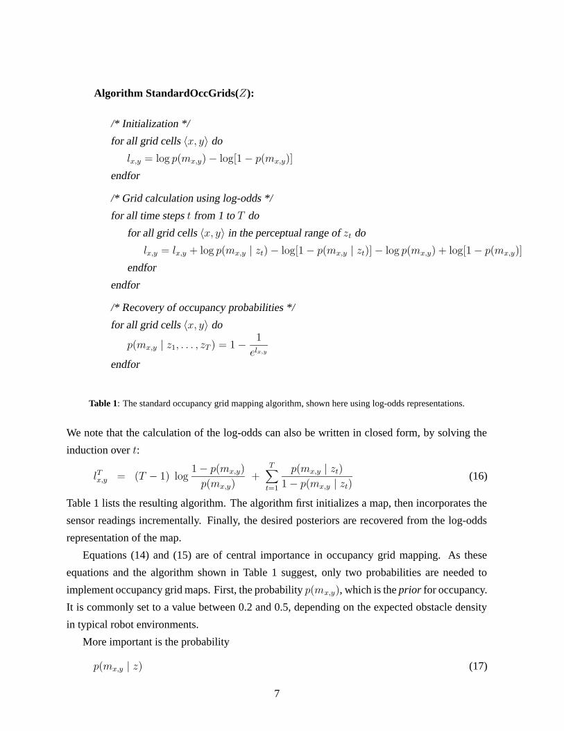
Table 1: The standard occupancy grid mapping algorithm, shown here using log-odds representations.

We note that the calculation of the log-odds can also be written in closed form, by solving the

induction over t:

lTx,y = (T − 1) log1 − p(mx,y)

p(mx,y)+

T∑

t=1

p(mx,y | zt)

1 − p(mx,y | zt)(16)

Table 1 lists the resulting algorithm. The algorithm first initializes a map, then incorporates the

sensor readings incrementally. Finally, the desired posteriors are recovered from the log-odds

representation of the map.

Equations (14) and (15) are of central importance in occupancy grid mapping. As these

equations and the algorithm shown in Table 1 suggest, only two probabilities are needed to

implement occupancy grid maps. First, the probability p(mx,y), which is the prior for occupancy.

It is commonly set to a value between 0.2 and 0.5, depending on the expected obstacle density

in typical robot environments.

More important is the probability

p(mx,y | z) (17)

7

which specifies the probability of occupancy of the grid cell mx,y conditioned on the measure-

ment z. This probability constitutes an inverse sensor model, since it maps sensor measurements

back to its causes. Occupancy grid maps commonly rely on such inverse models. Notice that

the inverse model does not take the occupancy of neighboring cells into account: It makes the

crucial independence assumption that the occupancy of a cell can be predicted regardless of a

cell’s neighbors. Herein lies a major problem of the standard occupancy approach, which leads

to the phenomena discussed in the introduction to this article. In fact, the problem is common to

any occupancy mapping algorithm that updates grid cells independently, regardless whether the

update is multiplicative, additive, or of any other form.

3 Occupancy Grid Mapping with Forward Models

This section presents our alternative approach to computing occupancy grid maps. The key idea

is to use forward models in place of the inverse models discussed in the previous section. For-

ward models enable us to calculate the likelihood of the sensor measurements for each map and

set of robot poses, in a way that considers all inter-cell dependencies. Mapping, thus, becomes

an optimization problem, which is the problem of finding the map that maximizes the data like-

lihood. This optimization problem can be carried out in the original high-dimensional space of

all maps, hence does not require the same decomposition into grid cell-specific problems found

in the standard occupancy grid mapping literature.

3.1 Forward Model: Intuitive Description

The key ingredient of our approach is a forward model. A forward model is a generative de-

scription of the physics of the sensors. Put probabilistically, a forward model is of the form

p(z | m) (18)

where z is a sensor measurement and m is the map. In other words, a forward model specifies a

probability distribution over sensor measurements z given a map m. As before, we assume that

the robot poses are known and part of z.

The specific forward model used in our implementation is quite simplistic. It models two

basic causes of sensor measurements:

1. The non-random case. Each occupied cell in the cone of a sensor has a probability

phit of reflecting a sonar beam. If a sonar beam is reflected back into the sensor, the

8

measurement is distorted by Gaussian noise. Of course, the nearest occupied grid cell has

the highest probability of being detected, followed by the second nearest, and so on. In

other words, the detection probability is distributed according to a geometric distribution

with parameter phit, convolved with Gaussian noise.

2. The random case. With probability prand, a sonar reading is random, drawn from a uni-

form distribution over the entire measurement range. In our simplistic sensor model, the

possibility that a sonar reading is random captures all unmodeled effect, such as specular

reflections, spurious readings, etc.

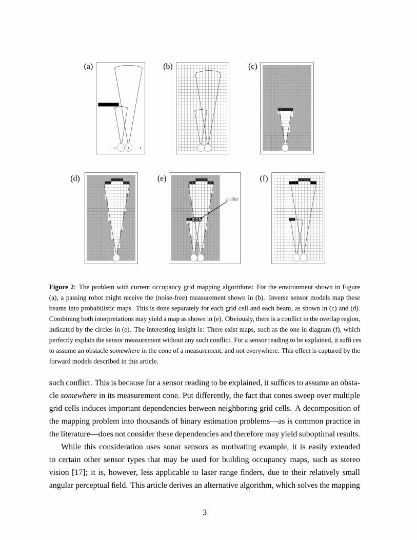
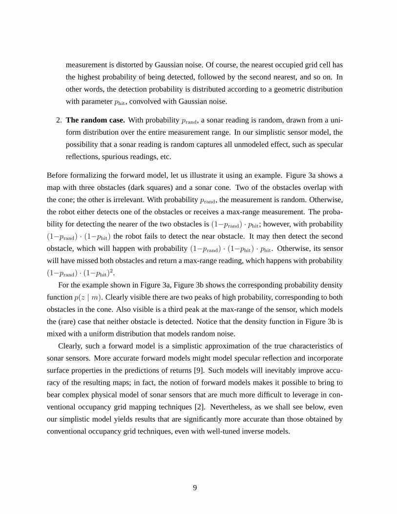
Before formalizing the forward model, let us illustrate it using an example. Figure 3a shows a

map with three obstacles (dark squares) and a sonar cone. Two of the obstacles overlap with

the cone; the other is irrelevant. With probability prand, the measurement is random. Otherwise,

the robot either detects one of the obstacles or receives a max-range measurement. The proba-

bility for detecting the nearer of the two obstacles is (1−prand) · phit; however, with probability

(1−prand) · (1−phit) the robot fails to detect the near obstacle. It may then detect the second

obstacle, which will happen with probability (1−prand) · (1−phit) · phit. Otherwise, its sensor

will have missed both obstacles and return a max-range reading, which happens with probability

(1−prand) · (1−phit)2.

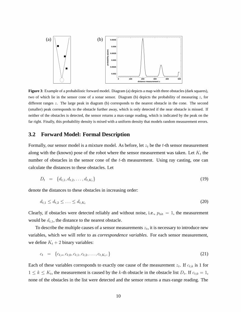
For the example shown in Figure 3a, Figure 3b shows the corresponding probability density

function p(z | m). Clearly visible there are two peaks of high probability, corresponding to both

obstacles in the cone. Also visible is a third peak at the max-range of the sensor, which models

the (rare) case that neither obstacle is detected. Notice that the density function in Figure 3b is

mixed with a uniform distribution that models random noise.

Clearly, such a forward model is a simplistic approximation of the true characteristics of

sonar sensors. More accurate forward models might model specular reflection and incorporate

surface properties in the predictions of returns [9]. Such models will inevitably improve accu-

racy of the resulting maps; in fact, the notion of forward models makes it possible to bring to

bear complex physical model of sonar sensors that are much more difficult to leverage in con-

ventional occupancy grid mapping techniques [2]. Nevertheless, as we shall see below, even

our simplistic model yields results that are significantly more accurate than those obtained by

conventional occupancy grid techniques, even with well-tuned inverse models.

9

� 0 100 200 300 400 500distance measurement z

0.002

0.0025

0.003

0.0035

0.004

0.0045

pro

bab

ility

p(z

|m)

(a) (b)

Figure 3: Example of a probabilistic forward model. Diagram (a) depicts a map with three obstacles (dark squares),

two of which lie in the sensor cone of a sonar sensor. Diagram (b) depicts the probability of measuring z, for

different ranges z. The large peak in diagram (b) corresponds to the nearest obstacle in the cone. The second

(smaller) peak corresponds to the obstacle further away, which is only detected if the near obstacle is missed. If

neither of the obstacles is detected, the sensor returns a max-range reading, which is indicated by the peak on the

far right. Finally, this probability density is mixed with a uniform density that models random measurement errors.

3.2 Forward Model: Formal Description

Formally, our sensor model is a mixture model. As before, let zt be the t-th sensor measurement

along with the (known) pose of the robot where the sensor measurement was taken. Let Kt the

number of obstacles in the sensor cone of the t-th measurement. Using ray casting, one can

calculate the distances to these obstacles. Let

Dt = {dt,1, dt,2, . . . , dt,Kt} (19)

denote the distances to these obstacles in increasing order:

dt,1 ≤ dt,2 ≤ . . . ≤ dt,Kt(20)

Clearly, if obstacles were detected reliably and without noise, i.e., phit = 1, the measurement

would be dt,1, the distance to the nearest obstacle.

To describe the multiple causes of a sensor measurements zt, it is necessary to introduce new

variables, which we will refer to as correspondence variables. For each sensor measurement,

we define Kt + 2 binary variables:

ct = {ct,∗, ct,0, ct,1, ct,2, . . . , ct,Kt, } (21)

Each of these variables corresponds to exactly one cause of the measurement zt. If ct,k is 1 for

1 ≤ k ≤ Kt, the measurement is caused by the k-th obstacle in the obstacle list Dt. If ct,0 = 1,

none of the obstacles in the list were detected and the sensor returns a max-range reading. The

10

random variable ct,∗ corresponds to the case where a measurement was purely random. Thus,

for each measurement zt exactly one of those variables is 1, all others are 0.

Each of these correspondences define a different probability distribution over the sensor

measurements zt. In the case that the k-th obstacle in Dt caused the measurement, that is,

ct,k = 1, we have a straightforward Gaussian noise variable centered at the range dt,k:

p(zt | m, ct,k = 1) =1√

2πσ2e−

12

(zt−dt,k)2

σ2 (22)

Here σ is the variance of the noise. If the measurement is entirely random, we obtain a uniform

distribution:

p(zt | m, ct,∗ = 1) =1

zmax

(23)

where zmax denotes the maximum sensor range. It will be convenient to write this probability as

follows:

p(zt | m, ct,∗ = 1) =1√

2πσ2e−

12

logz2max

2πσ2 (24)

The advantage of this notation is its similarity to the Gaussian noise case.

Finally, the sensor measurement might be caused by missing all obstacles in the cone, hence

becomes a max-range reading. We will describe this by a Gaussian centered on zmax:

p(zt | m, ct,0 = 1) =1√

2πσ2e−

12

(zt−zmax)2

σ2 (25)

We can now merge all these different causes together into a single likelihood function. Recall

that ct denotes the set of all correspondence variables for the measurement zt.

p(zt | m, ct) =1√

2πσ2e− 1

2

[

ct,∗ logz2max

2πσ2 +∑Kt

k=1ct,k

(zt−dt,k)2

σ2 +ct,0(zt−zmax)2

σ2

]

(26)

Notice that in Equation (26), exactly one of the correspondence variables in ct is 1. Thus, for

each of those possibilities, this equation reduces to one of the noise models outlined above.

Equation (26) calculates the probability of a sensor measurement zt if its cause is known,

via the correspondence variable ct. In practice, we are of cause not told what obstacle, if any,

was detected. Put differently, the correspondence variables are latent. All we have are range

measurements zt. It is therefore convenient to calculate the joint probability over measurements

and correspondences ct, which is obtained as follows:

p(zt, ct | m) = p(zt | m, ct) p(ct | m)

= p(zt | m, ct) p(ct) (27)

11

Here p(ct) is the prior over correspondences, which describes how likely each possible cor-

respondence is. We already informally described the prior in the previous section, where we

argued that the probability of receiving a random reading is prand, and the probability of detect-

ing an obstacle in the non-random case is phit for each obstacle in the sensor cone. Put formally,

we obtain

p(ct) =

prand if ct,∗ = 1

(1−prand)(1−phit)Kt if ct,0 = 1

(1−prand)(1−phit)k−1phit if ct,k = 1 for k ≥ 1

(28)

which defines the mixture uniform-geometric distribution discussed above.

3.3 Expected Data Log-Likelihood

To find the most likely map, we now have to define the data likelihood. In accordance with

the statistical literature, we will define the log-likelihood of the data, exploiting the observation

that maximizing the log-likelihood is equivalent to maximizing the likelihood (the logarithm is

strictly monotonic).

First, let us define the probability of all data. Above, we formulated the probability of a

single measurement zt. As above, our approach makes a static world assumption, but it does not

make the strong independence assumption of the standard occupancy grid mapping approach

discussed above. This enables us to write the likelihood of all data and correspondences as the

following product:

p(Z,C | m) =∏

t

p(zt, ct | m) (29)

Here Z denotes the set of all measurements (including poses), and C is the set of all correspon-

dences ct for all data. The logarithm of this expression is given by

log p(Z,C | m) =∑

t

log p(zt, ct | m) (30)

Finally, we notice that we are not really interested in calculating the probability of the corre-

spondence variables, since those are unobservable. Hence, we integrate those out by calculating

the expectations of the log-likelihood:

E[log p(Z,C | m) | Z,m] (31)

Here the expectation E is taken over all correspondence variables. The expected log-likelihood

of the data is the function that is being optimized in our approach. We obtain the expected

12

log-likelihood from Equation(31) by substituting Equations (30), (27), and (26), as indicated:

E[log p(Z,C | m) | Z,m]

(30)= E

{

∑

t

log p(zt, ct | m)

∣

∣

∣

∣

∣

Z,m]

}

(27)= E

{

∑

t

log p(zt | ct,m) p(ct)

∣

∣

∣

∣

∣

Z,m

}

(26)= E

{

∑

t

[

log p(ct) + log1√

2πσ2− 1

2

[

ct,∗ logz2max

2πσ2

+ct,0(zt − zmax)

2

σ2+

Kt∑

k=1

ct,k

(zt − dt,k)2

σ2

]]∣

∣

∣

∣

∣

Z,m

}

(32)

Exploiting the linearity of the expectation E, we obtain:

E[log p(Z,C | m) | Z,m]

=∑

t

[

E[log p(ct) | zt,m] + log1√

2πσ2− 1

2

[

E[ct,∗ | zt,m] logz2max

2πσ2

+E[ct,0 | zt,m](zt − zmax)

2

σ2+

Kt∑

k=1

E[ct,k | zt,m](zt − dt,k)

2

σ2

]]

(33)

The goal of mapping is to maximize this log-likelihood. Obviously, the map m and the ex-

pectations E[ct,∗ | zt,m], E[ct,0 | zt,m], and E[ct,k | zt,m] all interact. A common way to

optimize functions like the one considered here is the expectation maximization algorithm (in

short: EM) [6], which will be described in turn. As we will see, most terms in this log-likelihood

function can be ignored in the EM solution to this problem.

3.4 Finding Maps via EM

EM is an iterative algorithm that gradually maximizes the expected log-likelihood [13, 18]. Ini-

tially, EM generates a random map m. It then iterates two steps, an E-step, and an M-step, which

stand for expectation step and maximization step, respectively. In the E-step, the expectations

over the correspondences are calculated conditioned on a fixed map. The M-step calculates the

most likely map based on these expectations. Iterating both steps leads to a sequence of maps

that performs hill climbing in the expected log-likelihood space [13, 18].

In detail, we have:

1. Initialization. Maps in EM are discrete: Each grid cell is either occupied or free. There

is no notion of uncertainty in the map at this level, since EM finds the most likely map—

unlike conventional occupancy grid mapping algorithms, which estimates posteriors. In

13

principle, maps can be initialized randomly. However, we observed empirically that using

entirely unoccupied maps as initial maps worked best in terms of convergence speed.

2. E-step. For a given map m and measurements and poses Z, the E-step calculates the

expectations for the correspondences conditioned on m and Z. These expectations are the

probabilities for each of the possible causes of the sensor measurements:

et,∗ := E[ct,∗ | zt,m]

= p(ct,∗ = 1 | m, zt)

=1

p(zt | m)p(zt | m, ct,∗ = 1) p(ct,∗ = 1 | m)

=1

p(zt | m)

1

zmax

prand

=1

p(zt | m)√

2πσ2prand

√2πσ2

zmax

= η prand

√2πσ2

zmax

(34)

Here we defined

η =1

p(zt | m)√

2πσ2(35)

As we will see below, the variable η is a factor in every single expectation. In particular,

we have for 1 ≤ k ≤ Kt:

et,k := E[ct,k | zt,m]

= p(ct,k = 1 | m, zt)

=1

p(zt | m)p(zt | m, ct,k = 1) p(ct,k = 1 | m)

=1

p(zt | m)

1√2πσ2

e−12

(zt−dt,k)2

σ2 (1 − prand)(1 − phit)k−1phit

=1

p(zt | m)√

2πσ2(1 − prand)(1 − phit)

k−1phit e−12

(zt−dt,k)2

σ2

= η (1 − prand)(1 − phit)k−1phit e−

12

(zt−dt,k)2

σ2 (36)

Notice that the normalizer η is the same as in Equation (34). Finally, we obtain for the

correspondence variable ct,0:

et,0 := E[ct,0 | zt,m]

14

= p(ct,0 = 1 | m, zt)

=1

p(zt | m)p(zt | m, ct,0 = 1) p(ct,0 = 1 | m)

=1

p(zt | m)

1√2πσ2

e−12

(zt−zmax)2

σ2 (1 − prand)(1 − phit)Kt

=1

p(zt | m)√

2πσ2(1 − prand)(1 − phit)

Kt e−12

(zt−zmax)2

σ2

= η (1 − prand)(1 − phit)Kt e−

12

(zt−zmax)2

σ2 (37)

Notice that below, we will only use the expectations E[ct,k | zt,m]. However, the the other

two expectations are needed for calculating the normalization constant η. In particular, η

can be calculated from (34), (36), and (37) as follows:

η =

{

prand

√2πσ2

zmax

+ (1 − prand)(1 − phit)Kt e−

12

(zt−zmax)2

σ2

+Kt∑

k=1

[

(1 − prand)(1 − phit)k−1phit e−

12

(zt−dt,k)2

σ2

]}−1

(38)

Thus, η is a normalizer that is being applied to all correspondence variables at time t.

3. M-step. The M-step regards all expectations as constant relative to the optimization prob-

lem of finding the most likely map. Substituting in the expectations calculated in the

E-step, the expected log-likelihood (33) becomes:

E[log p(Z,C | m) | Z,m]

=∑

t

[

const. + log1√

2πσ2− 1

2

[

et,∗ logz2max

2πσ2

+et,0(zt − zmax)

2

σ2+

Kt∑

k=1

et,k

(zt − dt,k)2

σ2

]]

(39)

When determining a new map m, all but the last term on this expression can be omitted in

the optimization. In particular, the only remaining the model asserts on the expected log-

likelihood is through the obstacle ranges dt,k, which are calculated using the map. This

results in the greatly simplified minimization problem:

∑

t

Kt∑

k=1

et,k (zt − dt,k)2 −→ min (40)

15

The minimization of this expression is performed by hill climbing in the space of all maps.

More specifically, the (discrete) occupancy of individual grid cells is flipped whenever

doing so decreases the target function (40). This discrete search is terminated when no

additional flipping can further decrease the target function.

Implemented in the straightforward way, this approach can turn occupied grid cells into

unoccupied ones in the map, but it cannot do the opposite: turning free cells into occu-

pied one. This is because for free cells, the list of ranges Dt lacks the corresponding

distance, and hence no expectation is calculated in the E-step. Our implementation, thus,

executes a “mini E-step” for any free grid cell that is evaluated in the M-step. This mini

E-step involves setting the cell temporarily to occupied, calculating the expectations of all

affected sensor measurements, and subsequently determining the likelihood maximizing

map (M-step). As argued below, this can be done efficiently using the appropriate data

structures.

Since our approach performs maximization in a finite space, it terminates after finitely

many steps. In practice, we found that maximizing (40) takes less than a minute on a

low-end PC for the types maps shown in this article. Empirically, we never observed that

our algorithm was trapped in a poor local minimum. However, the optimum is not always

unique.

3.5 Calculating the Residual Occupancy Uncertainty

EM generates a single map, composed of zero-one occupancy values. This map contains no

notion of posterior uncertainty. In many applications, it is beneficial to know how certain we are

in the map. Conventional occupancy grid maps achieve this by calculating the marginal posterior

probability p(mx,y | Z) for each grid cell, as stated in Equation (4). Unfortunately, calculating

such marginal posteriors is computationally intractable in our more general model. Hence, we

have to approximate. The essential idea of our approximation is to condition this marginal on

the map obtained by EM. Let m denote this map, and m−x,y the map m without the value for

the grid cell 〈x, y〉. Our approach calculates the following posterior:

p(mx,y | Z, m−x,y) (41)

This is the marginal posterior over a grid cell’s occupancy assuming that the remaining map

has been correctly recovered by EM. Before discussing the implications of this approximation,

we note that the probability (41) can be calculated very efficiently. In particular, we note that

16

p(mx,y | Z, m−x,y) depends only on a subset of all measurements, namely those whose mea-

surement cones include the grid cell 〈x, y〉. Denoting this subset by Zx,y, we can calculate the

desired marginal as follows:

p(mx,y | Z, m−x,y)

= p(mx,y | Zx,y, m−x,y)

=p(Zx,y | mx,y, m−x,y) p(mx,y | m−x,y)

p(Zx,y | m−x,y)

=p(Zx,y | mx,y, m−x,y) p(mx,y)

p(Zx,y | mx,y, m−x,y) p(mx,y) + p(Zx,y | mx,y, m−x,y) (1 − p(mx,y))(42)

The terms p(Z | mx,y, m−x,y) and p(Z | mx,y, m−x,y) express the likelihood of the measure-

ments under the assumptions that mx,y is occupied, or free, respectively. Below, it shall prove

convenient to rewrite (42) as log-odds:

logp(mx,y | Z, m−x,y)

1 − p(mx,y | Z, m−x,y)= log

p(Zx,y | mx,y, m−x,y) p(mx,y)

p(Zx,y | mx,y, m−x,y) (1 − p(mx,y))(43)

This log odds ratio is easily calculated from the sensor model (26). Our implementation main-

tains a list of relevant sensor measurements Zx,y for each grid cell 〈x, y〉, which makes it possible

to calculate the marginals for an entire map in a few seconds, even for the largest map shown in

this article.

Clearly, conditioning on the EM map m is only an approximation. In particular, it fails to

capture the residual uncertainty in the map by (falsely) asserting that the map found by EM is the

correct one. As a result, our estimates will be overly confident. To counter this overconfidence,

our approach mixes this estimate with the prior for occupancy, using a mixing parameter α. The

mixing rule is analogous to the update rule of the log odds ratio in in occupancy grid maps (14):

logqx,y

1 − qx,y

= α logp(mx,y | Z, m−x,y)

1 − p(mx,y | Z, m−x,y)+ (1 − α) log

p(mx,y)

1 − p(mx,y)(44)

Here qx,y denotes the final approximation of the marginal posterior. Solving this equation for q

gives us the following expression:

qx,y = 1 −

1 +

(

p(mx,y | Z, m−x,y)

1 − p(mx,y | Z, m−x,y)

)α (

p(mx,y)

1 − p(mx,y)

)1−α

−1

(45)

This approach combines two approximations with opposite error. If α = 1, the posterior estimate

is given by the the term p(mx,y | Z, m−x,y), This term will overestimate the confidence in the

value of mx,y. If α = 0, the posterior (45) is equivalent to the prior for occupancy p(mx,y). This

prior underestimates the confidence in the occupancy value, since it ignores the measurements

17

Z. This consideration suggests that an “optimal” α exist for each grid cell, which would provide

the best approximation to the posterior probability under our model. However, computing this

α is intractable; hence we simply set one by hand.

3.6 The Mapping Algorithm with Forward Models

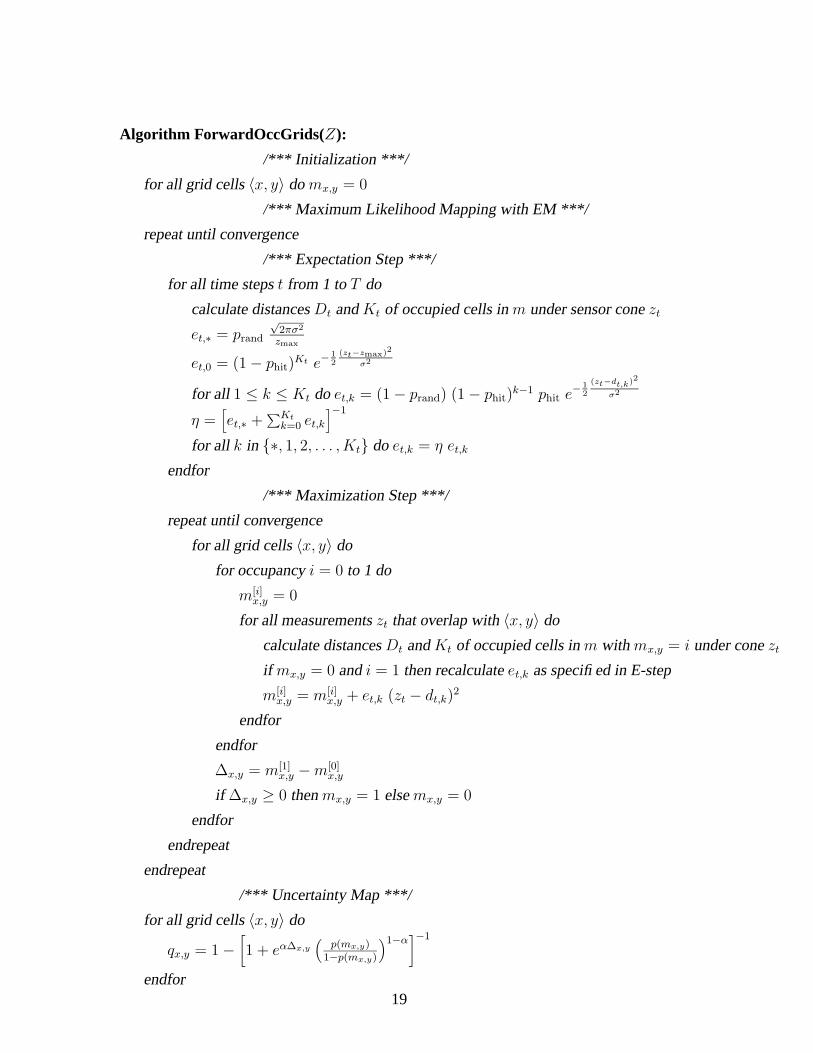
Table 2 summarizes the final algorithm for learning occupancy grid maps using forward models.

The algorithm consists of three parts: The initialization, the EM optimization, and a final step

that extracts the uncertainty map.

Our implementation uses an efficient data structure for cross-linking sensor measurements

zt and grid cells 〈x, y〉. A doubly-linked list makes it possible to match measurements and grid

cells highly efficiently, without the necessity to search through long lists of grid coordinates,

or sensor measurements. Moreover, when calculating the differences ∆x,y, only terms in the

expected log-likelihood are considered that actually depend on the grid cell 〈x, y〉. By doing so,

the inner loops of the algorithm are highly efficient, making it possible to generate maps within

less than a minute.

As stated at several locations in this article, the advantage of our new algorithm is that it

overcomes a critical independence assumption between neighboring grid cells, commonly made

in the existing literature on occupancy grid mapping. On the downside, we note that this new

occupancy grid mapping algorithm is not incremental. Instead, multiple passes through the data

are necessary to find a maximum likelihood map. This is a disadvantage relative to the stan-

dard occupancy grid mapping algorithm, which can incorporate data incrementally. However,

for moderately sized data sets we found that our algorithm takes less than a minute—which is

significantly faster than the process of data collection.

4 Experimental Results

Our approach was successfully applied to learning grid maps using simulated and real robot

data. Since localization during mapping is not the focus of the current article, we assumed that

pose estimates were available. In the simulator, these were easily obtained. For the real world

data, we relied on the concurrent mapping and localization algorithm described in [25].

Our main findings are that our approach does a better job resolving conflicts among different

range measurements. Those are particularly prevalent in discontinuous environment, such as

environment with small openings (doors). They also arise in cases with high degrees of noise,

18

Algorithm ForwardOccGrids(Z):

/*** Initialization ***/

for all grid cells 〈x, y〉 do mx,y = 0

/*** Maximum Likelihood Mapping with EM ***/

repeat until convergence

/*** Expectation Step ***/

for all time steps t from 1 to T do

calculate distances Dt and Kt of occupied cells in m under sensor cone zt

et,∗ = prand

√2πσ2

zmax

et,0 = (1 − phit)Kt e−

12

(zt−zmax)2

σ2

for all 1 ≤ k ≤ Kt do et,k = (1 − prand) (1 − phit)k−1 phit e−

12

(zt−dt,k)2

σ2

η =[

et,∗ +∑Kt

k=0 et,k

]−1

for all k in {∗, 1, 2, . . . , Kt} do et,k = η et,k

endfor

/*** Maximization Step ***/

repeat until convergence

for all grid cells 〈x, y〉 do

for occupancy i = 0 to 1 do

m[i]x,y = 0

for all measurements zt that overlap with 〈x, y〉 do

calculate distances Dt and Kt of occupied cells in m with mx,y = i under cone zt

if mx,y = 0 and i = 1 then recalculate et,k as specified in E-step

m[i]x,y = m[i]

x,y + et,k (zt − dt,k)2

endfor

endfor

∆x,y = m[1]x,y − m[0]

x,y

if ∆x,y ≥ 0 then mx,y = 1 else mx,y = 0

endfor

endrepeat

endrepeat

/*** Uncertainty Map ***/

for all grid cells 〈x, y〉 do

qx,y = 1 −[

1 + eα∆x,y

(

p(mx,y)1−p(mx,y)

)1−α]−1

endfor

Table 2: The new occupancy grid mapping algorithm with forward models.

19

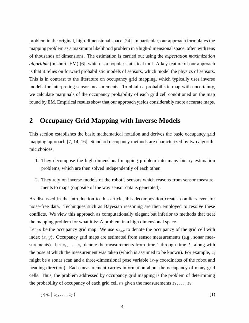
(a) raw data (example)

First simulation run: 1 measurement of the open door(b) Conventional algorithm (c) ML map (d) Map with uncertainty

Second: Simulation run: 3 measurements of the open door(e) Conventional algorithm (f) ML map (g) Map with uncertainty

Third simulation run: 16 measurements of the open door(h) Conventional algorithm (i) ML map (j) Map with uncertainty

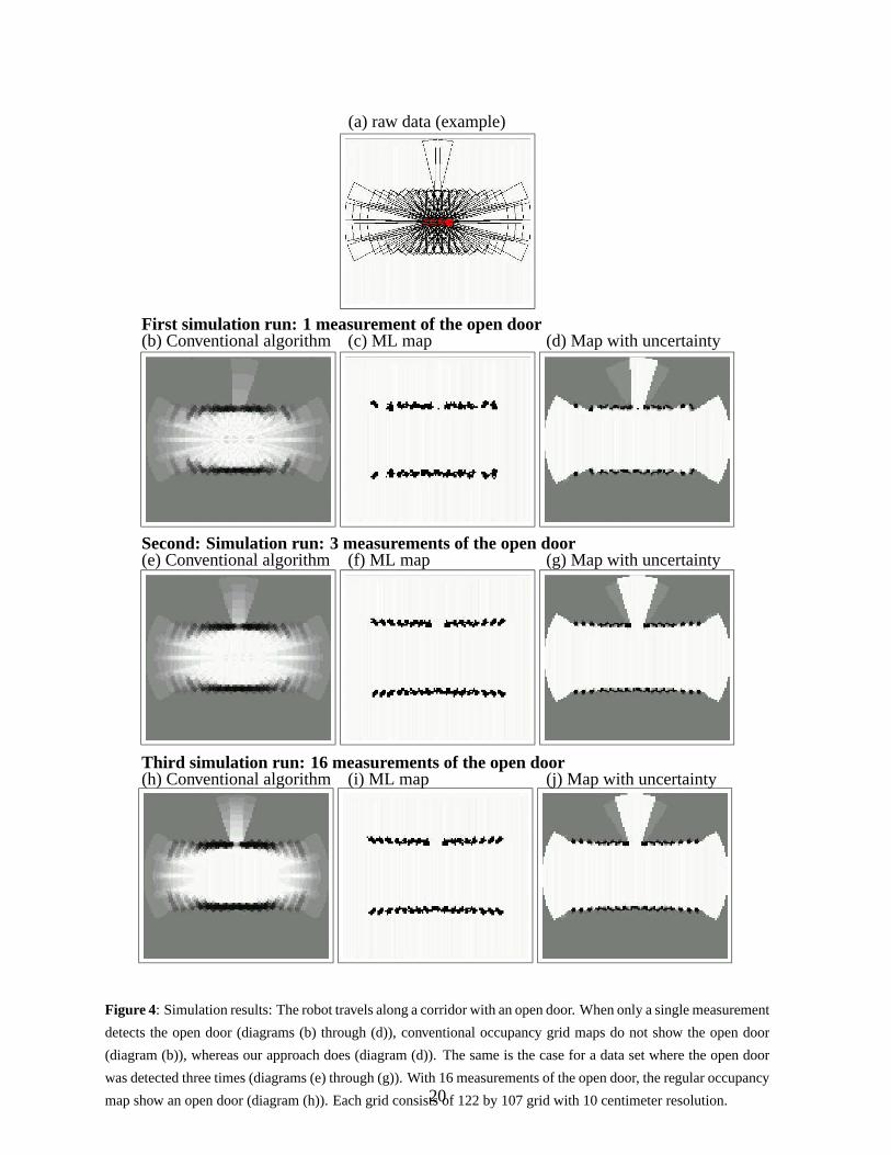
Figure 4: Simulation results: The robot travels along a corridor with an open door. When only a single measurement

detects the open door (diagrams (b) through (d)), conventional occupancy grid maps do not show the open door

(diagram (b)), whereas our approach does (diagram (d)). The same is the case for a data set where the open door

was detected three times (diagrams (e) through (g)). With 16 measurements of the open door, the regular occupancy

map show an open door (diagram (h)). Each grid consists of 122 by 107 grid with 10 centimeter resolution.20

(a) (b) (c)

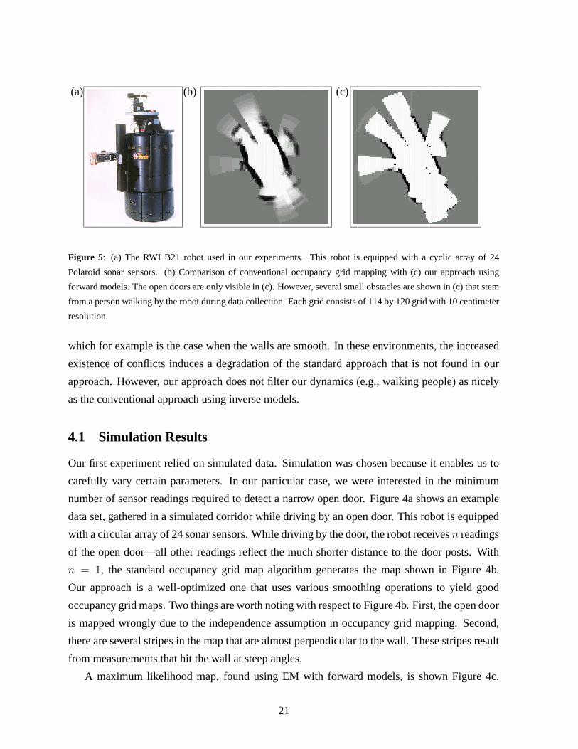
Figure 5: (a) The RWI B21 robot used in our experiments. This robot is equipped with a cyclic array of 24

Polaroid sonar sensors. (b) Comparison of conventional occupancy grid mapping with (c) our approach using

forward models. The open doors are only visible in (c). However, several small obstacles are shown in (c) that stem

from a person walking by the robot during data collection. Each grid consists of 114 by 120 grid with 10 centimeter

resolution.

which for example is the case when the walls are smooth. In these environments, the increased

existence of conflicts induces a degradation of the standard approach that is not found in our

approach. However, our approach does not filter our dynamics (e.g., walking people) as nicely

as the conventional approach using inverse models.

4.1 Simulation Results

Our first experiment relied on simulated data. Simulation was chosen because it enables us to

carefully vary certain parameters. In our particular case, we were interested in the minimum

number of sensor readings required to detect a narrow open door. Figure 4a shows an example

data set, gathered in a simulated corridor while driving by an open door. This robot is equipped

with a circular array of 24 sonar sensors. While driving by the door, the robot receives n readings

of the open door—all other readings reflect the much shorter distance to the door posts. With

n = 1, the standard occupancy grid map algorithm generates the map shown in Figure 4b.

Our approach is a well-optimized one that uses various smoothing operations to yield good

occupancy grid maps. Two things are worth noting with respect to Figure 4b. First, the open door

is mapped wrongly due to the independence assumption in occupancy grid mapping. Second,

there are several stripes in the map that are almost perpendicular to the wall. These stripes result

from measurements that hit the wall at steep angles.

A maximum likelihood map, found using EM with forward models, is shown Figure 4c.

21

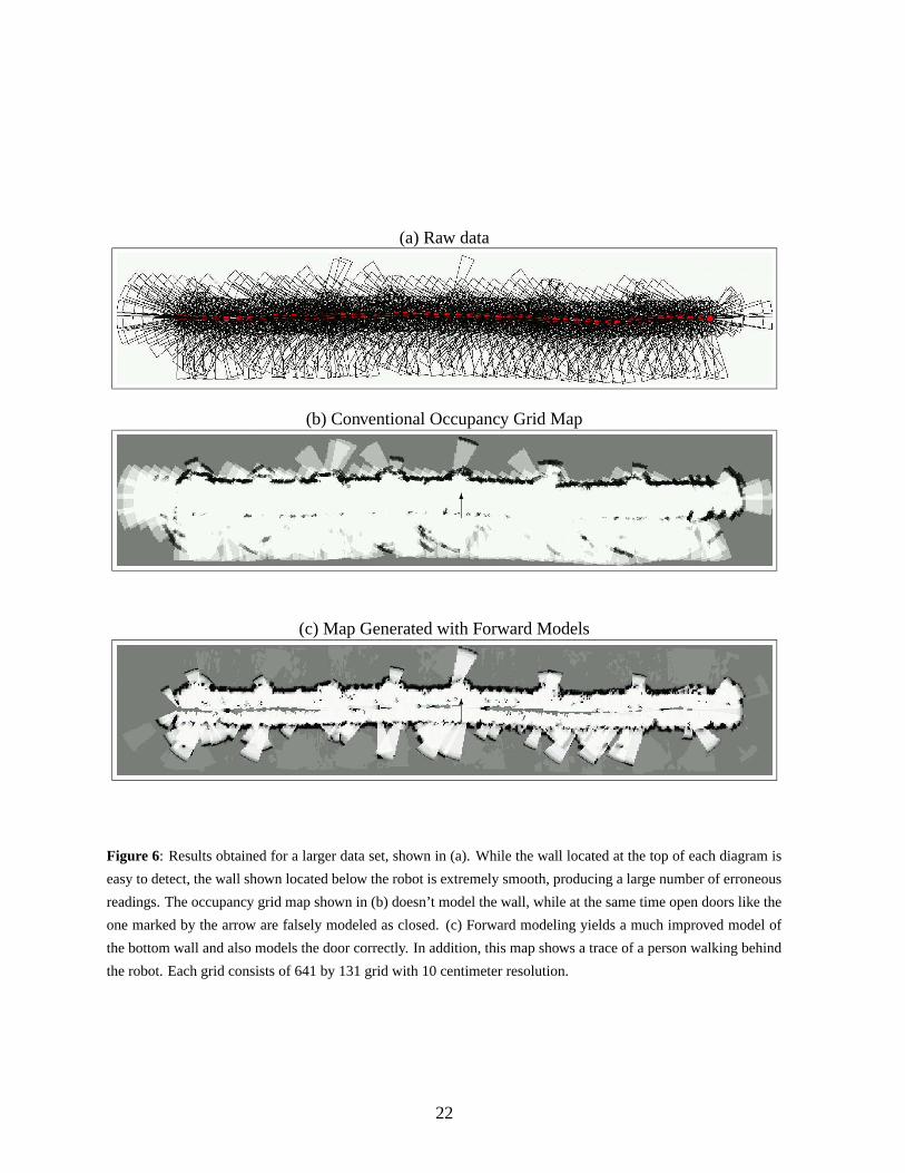
(a) Raw data

(b) Conventional Occupancy Grid Map

6

(c) Map Generated with Forward Models

6

Figure 6: Results obtained for a larger data set, shown in (a). While the wall located at the top of each diagram is

easy to detect, the wall shown located below the robot is extremely smooth, producing a large number of erroneous

readings. The occupancy grid map shown in (b) doesn’t model the wall, while at the same time open doors like the

one marked by the arrow are falsely modeled as closed. (c) Forward modeling yields a much improved model of

the bottom wall and also models the door correctly. In addition, this map shows a trace of a person walking behind

the robot. Each grid consists of 641 by 131 grid with 10 centimeter resolution.

22

Clearly, the most likely solution possesses an open door. In fact, the result of our algorithm does

not attribute any of the sensor reading to a random error event. Instead, all of the sensor readings

are perfectly well explained with this map! Figure 4d shows the uncertainty map extracted from

the maximum likelihood map using our posterior approximation. Again, this map correctly

features an open door, confirming our basic conjecture that our approach is superior in handling

seemingly inconsistent sensor measurements.

The basic experiment was repeated for different values of n. As n increases, the evidence

for an open door increases, and ultimately even the standard occupancy grid mapping algorithm

will preclude a map with an open door. The bottom two rows of Figure 4 show results for n = 3,

and n = 16, respectively. For n = 3, the evidence for the existence of an open door is high, yet

the standard approach still shows no door, due to the large number of readings that suggest the

existence of an obstacle in the door region. Finally, for n = 16, the door is visible even for the

conventional approach, although not as clearly as for our new approach.

The interesting observation here is while the standard occupancy grid mapping algorithm

uses probabilistic means to accommodate inconsistent sensor interpretations, there are no such

conflicts in our approach. All data sets are perfectly explained by any of the maximum likelihood

maps shown in Figure 4.

4.2 Real World Results

Real world results were obtained using a RWI B21 robot equipped with 24 sonar sensors, shown

in Figure 5a. We collected two data sets, both of which possessed unique challenges.

The first data set, documented in Figure 5b&c, compares the standard occupancy grid map-

ping algorithm to the one using forward models. In this data set, there are two narrow open

doors on either side. As predicted by the simulation, the doors are only visible in the forward

modeling approach, whose results are shown in Figure 5c. Several dots in the EM map stem

from the fact that a person walked by the robot during data collection. This highlights one of the

nice features of standard occupancy grid maps, which typically do not show traces of people as

long as they do not remain at a single location in the majority of measurements. However, our

approach overall a much better job describing the environment.

The final and most interesting data set is much larger. Figure 6a shows a robot trace in a

50 meters long corridor. This corridor is quite challenging: On the one hand, there are several

open doors on one side. On the other, one of the walls is extremely smooth, resulting in a large

number of erroneous readings. The level of noise is so high that the standard occupancy grid

23

approach plainly fails to detect and model the wall, as shown in Figure 6b. At the same time,

it also fails to detect open doors, as indicated by the arrow in Figure 6b. This is interesting,

since we have a natural trade-off: By adjusting the gain so as to pay more attention to occupied

regions, the wall eventually becomes visible by the doors will be entirely closed. By adjusting

the gain into the opposite direction, the doors will eventually become visible but the wall will be

missing entirely.

As Figure 6c suggests, our approach succeeds in finding at least some of the wall, while

modeling the openings correctly. However, our approach shows the trace of the person control-

ling the robot with a joystick. The presence of the person violates the static world assumption

that underlies both families of occupancy grid mapping algorithms; however, our approach gen-

erates maps that explain the corresponding readings (but do not look as nice in this regard).

Nevertheless, the ability to model both the doors and walls more accurately than the standard

approach suggests that our approach is superior in situations with seemingly conflicting range

measurements. Generating maps of the size shown here typically takes less than a minute on a

low-end PC.

5 Discussion

This article presented an algorithm for generating occupancy grid maps which relies on phys-

ical forward models. Instead of breaking down the map learning problem into a multitude of

independent binary estimation problems—as is the case in existing occupancy grid mapping

algorithms—our approach searches maps in the high-dimensional space. To perform this search,

we have adopted the popular EM algorithm to the map estimation problem. The EM algorithm

identifies a plausible map by gradually maximizing the likelihood of all measurements in a hill-

climbing fashion. Uncertainty maps are obtained by calculating marginal probabilities, similar

to those computed by conventional occupancy grid mapping techniques.

Our approach has two main advantages over conventional occupancy grid mapping tech-

niques: First, we believe forward models are more natural to obtain than inverse models, since

forward models are descriptive of the physical phenomena that underlie the data generation.

Second, and more importantly, our approach yields more consistent maps. This is because our

approach relies on fewer independence assumptions. It treats the mapping problem for what it

is: A search in a high dimensional space. The disadvantages of our approach are an apparent

increased sensitivity to changes in the environment, and a need to go through the data mul-

24

tiple times, which prohibits its real-time application. Extending this algorithm into an online

algorithm is subject of future research (see [18]).

Experimental results illustrate that more accurate maps can be built in situations with seem-

ingly conflicting sensor information. Such situations include environments with narrow open-

ings and environments were sonars frequently fail to detect obstacles. These advantages are

counterbalanced by two of the limitations of our approach: First, dynamic obstacles show up

more frequently in our approach, and second, our approach is not real-time.

In a recent article [8], we extended the basic EM approach to accommodate pose uncertainty

and environment dynamics. We have successfully demonstrated that the algorithm described

here can be extended to yield significantly more accurate maps and robot pose estimates in the

presence of moving objects. The key extension here is to include the robot pose variables in the

set of latent variables. In the present article, those are obtained through a separate algorithm [25]

and simply assumed to be correct. Furthermore, the implementation in [8] employs laser range

finders, whose accuracy greatly facilitates the identification of inconsistent sensor measurements

when compared to the sonar sensors used in the present article.

As discussed further above, the sensor models used in our implementation are highly sim-

plistic. They do not model many common phenomena in sonar-based range sensing, such as

indirect readings caused by specular reflection, or obstacle detection in a sensor’s side cone. In

principle, the forward modeling approach makes it possible to utilize any probabilistic sensor

model, such as the one in [2]. We conjecture that improved sensor models will lead to better

mapping results.

Another opportunity for future research arises from the fact that environments possess struc-

ture. The prior probability in our approach (and in conventional occupancy grid mapping tech-

niques) assumes independence between different grid cells. In reality, this is just a crude ap-

proximation. Environments are usually composed of larger objects, such as walls, furniture,

etc. Mapping with forward models facilitate the use of more informed priors, as shown in [12].

However, the acquisition of adequate priors that characterize indoor environments is largely an

open research area.

Regardless of these limitations, we believe that our approach sheds light on an alternative

approach for building maps with mobile robots. We believe that by overcoming the classical

independence that forms the core of techniques based on inverse models, we can ultimately

arrive at more powerful mapping algorithms that generate maps of higher consistency with the

data. The evidence presented in this and various related papers suggests that forward models are

powerful tools for building maps of robot environments.

25

Acknowledgment

The author thanks Tom Minka, Andrew Y. Ng, and Zoubin Ghahramani for extensive discussions

concerning Bayesian approaches and variational approximations for occupancy grid mapping.

He also thanks Dirk Hahnel and Wolfram Burgard for discussions on how to apply this approach

to SLAM problems in dynamic environments.

This research is sponsored by by DARPA’s MARS Program (Contract number N66001-01-

C-6018 and NBCH1020014) and the National Science Foundation (CAREER grant number

IIS-9876136 and regular grant number IIS-9877033), all of which is gratefully acknowledged.

The views and conclusions contained in this document are those of the author and should not

be interpreted as necessarily representing official policies or endorsements, either expressed or

implied, of the United States Government or any of the sponsoring institutions.

References

[1] J. Borenstein and Y. Koren. The vector field histogram – fast obstacle avoidance for mobile

robots. IEEE Journal of Robotics and Automation, 7(3):278–288, June 1991.

[2] M.K. Brown. Feature extraction techniques for recognizing solid objects with an ultrasonic

range sensor. IEEE Journal of Robotics and Automation, RA-1(4), 1985.

[3] J. Buhmann, W. Burgard, A.B. Cremers, D. Fox, T. Hofmann, F. Schneider, J. Strikos, and

S. Thrun. The mobile robot Rhino. AI Magazine, 16(1), 1995.

[4] W. Burgard, D. Fox, H. Jans, C. Matenar, and S. Thrun. Sonar-based mapping of large-

scale mobile robot environments using EM. In Proceedings of the International Conference

on Machine Learning, Bled, Slovenia, 1999.

[5] W. Burgard, D. Fox, M. Moors, R. Simmons, and S. Thrun. Collaborative multi-robot

exploration. In Proceedings of the IEEE International Conference on Robotics and Au-

tomation (ICRA), San Francisco, CA, 2000. IEEE.

[6] A.P. Dempster, A.N. Laird, and D.B. Rubin. Maximum likelihood from incomplete data

via the EM algorithm. Journal of the Royal Statistical Society, Series B, 39(1):1–38, 1977.

[7] A. Elfes. Occupancy Grids: A Probabilistic Framework for Robot Perception and Navi-

gation. PhD thesis, Department of Electrical and Computer Engineering, Carnegie Mellon

University, 1989.

26

[8] D. Hahnel, R. Triebel, W. Burgard, and S. Thrun. Map building with mobile robots in

dynamic environments. Submitted for publication, 2002.

[9] A. Howard and L. Kitchen. Generating sonar maps in highly specular environments. In

Proceedings of the Fourth International Conference on Control Automation Robotics and

Vision, pages 1870–1874, 1996.

[10] K. Konolige and K. Chou. Markov localization using correlation. In Proceedings of the Six-

teenth International Joint Conference on Artificial Intelligence (IJCAI), Stockholm, Swe-

den, 1999. IJCAI.

[11] D. Kortenkamp, R.P. Bonasso, and R. Murphy, editors. AI-based Mobile Robots: Case

studies of successful robot systems, Cambridge, MA, 1998. MIT Press.

[12] Y. Liu, R. Emery, D. Chakrabarti, W. Burgard, and S. Thrun. Using EM to learn 3D models

with mobile robots. In Proceedings of the International Conference on Machine Learning

(ICML), 2001.

[13] G.J. McLachlan and T. Krishnan. The EM Algorithm and Extensions. Wiley Series in

Probability and Statistics, New York, 1997.

[14] H. P. Moravec. Sensor fusion in certainty grids for mobile robots. AI Magazine, 9(2):61–

74, 1988.

[15] H. P. Moravec and A. Elfes. High resolution maps from wide angle sonar. In Proc. IEEE

Int. Conf. Robotics and Automation, pages 116–121, 1985.

[16] H.P. Moravec and M.C. Martin. Robot navigation by 3D spatial evidence grids. Mobile

Robot Laboratory, Robotics Institute, Carnegie Mellon University, 1994.

[17] D. Murray and J. Little. Interpreting stereo vision for a mobile robot. Autonomous Robots,

2001. To Appear.

[18] R.M. Neal and G.E. Hinton. A view of the EM algorithm that justifies incremental, sparse,

and other variants. In M.I. Jordan, editor, Learning in Graphical Models. Kluwer Aca-

demic Press, 1998.

[19] B. Schiele and J. Crowley. A comparison of position estimation techniques using occu-

pancy grids. In Proceedings of the 1994 IEEE International Conference on Robotics and

Automation, pages 1628–1634, San Diego, CA, May 1994.

27

[20] R. Simmons. Where in the world is xavier, the robot? Machine Perception, 5(1), 1996.

[21] R. Simmons, D. Apfelbaum, W. Burgard, M. Fox, D. an Moors, S. Thrun, and H. Younes.

Coordination for multi-robot exploration and mapping. In Proceedings of the AAAI Na-

tional Conference on Artificial Intelligence, Austin, TX, 2000. AAAI.

[22] S. Thrun. Exploration and model building in mobile robot domains. In E. Ruspini, editor,

Proceedings of the IEEE International Conference on Neural Networks, pages 175–180,

San Francisco, CA, 1993. IEEE Neural Network Council.

[23] S. Thrun. Learning metric-topological maps for indoor mobile robot navigation. Artificial

Intelligence, 99(1):21–71, 1998.

[24] S. Thrun. Learning occupancy grids with forward models. In Proceedings of the Confer-

ence on Intelligent Robots and Systems (IROS’2001), Hawaii, 2001.

[25] S. Thrun, D. Fox, and W. Burgard. A probabilistic approach to concurrent mapping and

localization for mobile robots. Machine Learning, 31:29–53, 1998. also appeared in Au-

tonomous Robots 5, 253–271 (joint issue).

[26] B. Yamauchi. A frontier-based approach for autonomous exploration. In Proceedings

of the IEEE International Symposium on Computational Intelligence in Robotics and Au-

tomation, pages 146–151, Monterey, CA, 1997.

[27] B. Yamauchi, P. Langley, A.C. Schultz, J. Grefenstette, and W. Adams. Magellan: An

integrated adaptive architecture for mobile robots. Technical Report 98-2, Institute for the

Study of Learning and Expertise (ISLE), Palo Alto, CA, May 1998.

28