Embed Size (px)
Citation preview
HAL Id: tel-00982325https://tel.archives-ouvertes.fr/tel-00982325
Submitted on 23 Apr 2014
HAL is a multi-disciplinary open accessarchive for the deposit and dissemination of sci-entific research documents, whether they are pub-lished or not. The documents may come fromteaching and research institutions in France orabroad, or from public or private research centers.
L’archive ouverte pluridisciplinaire HAL, estdestinée au dépôt et à la diffusion de documentsscientifiques de niveau recherche, publiés ou non,émanant des établissements d’enseignement et derecherche français ou étrangers, des laboratoirespublics ou privés.
Stereo vision and LIDAR based Dynamic OccupancyGrid mapping : Application to scenes analysis for
Intelligent VehiclesYou Li
To cite this version:You Li. Stereo vision and LIDAR based Dynamic Occupancy Grid mapping : Application to scenesanalysis for Intelligent Vehicles. Computers and Society [cs.CY]. Université de Technologie de Belfort-Montbeliard, 2013. English. �NNT : 2013BELF0225�. �tel-00982325�
Thèse de Doctorat
n
é c o l e d o c t o r a l e s c i e n c e s p o u r l ’ i n g é n i e u r e t m i c r o t e c h n i q u e s
U N I V E R S I T É D E T E C H N O L O G I E B E L F O R T - M O N T B É L I A R D
Stereo Vision and Lidar basedDynamic Occupancy Grid MappingApplication to Scene Analysis for Intelligent Vehicles
YOU LI

Thèse de Doctorat
é c o l e d o c t o r a l e s c i e n c e s p o u r l ’ i n g é n i e u r e t m i c r o t e c h n i q u e s
U N I V E R S I T É D E T E C H N O L O G I E B E L F O R T - M O N T B É L I A R D
THESE presentee par
YOU LI
pour obtenir le
Grade de Docteur de
l’Universite de Technologie de Belfort-Montbeliard
Specialite : Informatique
Stereo Vision and Lidar based Dynamic Occupancy
Grid MappingApplication to Scene Analysis for Intelligent Vehicles
Soutenue publiquement le 03 December 2013 devant le Jury compose de :
SERGIU NEDEVSCHI Rapporteur Professeur a Technical University of Cluj-
Napoca (Roumanie)
MICHEL DEVY Rapporteur Directeur de Recherche CNRS a LAAS-
CNRS de Toulouse
HANZI WANG Rapporteur Professeur a Xiamen University (Chine)
VINCENT FREMONT Examinateur Maıtre de Confereces HDR a Universite de
Technologie de Compiegne
JEAN-CHARLES NOYER Examinateur Professeur a Universite du Littoral Cote
d’Opale
OLIVIER AYCARD Examinateur Maıtre de Confereces HDR a Universite de
Grenoble 1
CINDY CAPPELLE Examinateur Maıtre de Confereces a Universite de
Technologie de Belfort-Montbeliard
YASSINE RUICHEK Directeur de these Professeur a Universite de Technologie de
Belfort-Montbeliard
N◦ 2 2 5

Contents
1 Introduction 11.1 Background . . . . . . . . . . . . . . . . . . . . . . . . . . . . . . . . 1
1.2 Problem Statement . . . . . . . . . . . . . . . . . . . . . . . . . . . . 3
1.3 Experimental Platform . . . . . . . . . . . . . . . . . . . . . . . . . . 5
1.4 Structure of the manuscript . . . . . . . . . . . . . . . . . . . . . . . 5
2 Basic Knowledge 72.1 Sensor Models . . . . . . . . . . . . . . . . . . . . . . . . . . . . . . . 7
2.1.1 Coordinate Systems . . . . . . . . . . . . . . . . . . . . . . . 7
2.1.2 Lidar Measurement Model . . . . . . . . . . . . . . . . . . . . 8
2.1.3 Monocular Camera Measurement Model . . . . . . . . . . . . 9
2.1.4 Binocular Stereo Vision System Model . . . . . . . . . . . . . 13
2.2 Stereo Vision System Calibration . . . . . . . . . . . . . . . . . . . . 14
2.2.1 Intrinsic Calibration of a camera . . . . . . . . . . . . . . . . 14
2.2.2 Extrinsic Calibration of Binocular Vision System . . . . . . . 14
2.2.3 Image Undistortion and Stereo Recti�cation . . . . . . . . . . 15
2.2.4 Corner Points Triangulation . . . . . . . . . . . . . . . . . . . 17
2.3 Least Squares Estimation . . . . . . . . . . . . . . . . . . . . . . . . 19
2.3.1 Linear Least Squares . . . . . . . . . . . . . . . . . . . . . . . 20
2.3.2 Non-linear Least Squares . . . . . . . . . . . . . . . . . . . . 25
2.3.3 Robust Estimation methods . . . . . . . . . . . . . . . . . . . 28
2.4 Image Local Feature Detectors and Descriptors . . . . . . . . . . . . 30
2.4.1 Local Invariant Feature Detectors . . . . . . . . . . . . . . . . 30
2.4.2 Feature descriptors . . . . . . . . . . . . . . . . . . . . . . . . 39
2.4.3 Associating feature points through images . . . . . . . . . . . 43
2.5 Conclusion . . . . . . . . . . . . . . . . . . . . . . . . . . . . . . . . . 46
3 Stereo Vision based Ego-motion Estimation 473.1 Introduction . . . . . . . . . . . . . . . . . . . . . . . . . . . . . . . . 48
3.2 Circular Feature Points Detection and Association . . . . . . . . . . 50
3.2.1 Circular Feature Point Association by KLT Tracker . . . . . . 51
3.2.2 Circular Feature Point Association by Matching . . . . . . . . 51
3.3 Ego-motion Computation . . . . . . . . . . . . . . . . . . . . . . . . 54
3.3.1 3D-2D Constraint based Ego-motion Estimation . . . . . . . 54
3.4 Experiments of Stereo Visual Odometry . . . . . . . . . . . . . . . . 57
3.4.1 Comparing Di�erent Feature Association Approaches . . . . . 57
3.4.2 Stereo Visual Odometry in Urban Environment . . . . . . . . 62
3.5 Conclusion and Future Works . . . . . . . . . . . . . . . . . . . . . . 70
ii Contents
4 Independent Moving Object Detection, Segmentation and Recog-nition 714.1 Independent Moving Object Detection and Segmentation . . . . . . . 71
4.1.1 Introduction . . . . . . . . . . . . . . . . . . . . . . . . . . . . 71
4.1.2 UV-Disparity Based Independent Moving Objectxs Detection
and Segmentation . . . . . . . . . . . . . . . . . . . . . . . . 73
4.1.3 Experimental results of U-disparity image based Independent
Moving Object Detection . . . . . . . . . . . . . . . . . . . . 77
4.2 Moving Object Recognition using Spatial Information . . . . . . . . 80
4.2.1 Introduction . . . . . . . . . . . . . . . . . . . . . . . . . . . . 80
4.2.2 Spatial Feature Extraction and Classi�cation . . . . . . . . . 81
4.2.3 Experimental Results . . . . . . . . . . . . . . . . . . . . . . 84
4.3 Conclusion and Future Works . . . . . . . . . . . . . . . . . . . . . . 89
5 Extrinsic Calibration between a Stereo Vision System and a Lidar 915.1 Introduction . . . . . . . . . . . . . . . . . . . . . . . . . . . . . . . . 91
5.1.1 Related works . . . . . . . . . . . . . . . . . . . . . . . . . . . 92
5.1.2 Problem Formulation . . . . . . . . . . . . . . . . . . . . . . . 93
5.1.3 Performance Evaluation . . . . . . . . . . . . . . . . . . . . . 94
5.2 3D Plane Reconstruction based Extrinsic Calibration . . . . . . . . . 95
5.2.1 Corner Points Triangulation . . . . . . . . . . . . . . . . . . . 96
5.2.2 3D Plane Estimation . . . . . . . . . . . . . . . . . . . . . . . 96
5.2.3 Automatic Lidar Measurements Extraction . . . . . . . . . . 100
5.2.4 Estimating Rigid Transformation between the lidar and the
Stereoscopic System . . . . . . . . . . . . . . . . . . . . . . . 101
5.2.5 Summary of the Calibration Procedure . . . . . . . . . . . . . 103
5.3 Experimental Results . . . . . . . . . . . . . . . . . . . . . . . . . . . 104
5.3.1 Computer Simulations . . . . . . . . . . . . . . . . . . . . . . 104
5.3.2 Real Data Test . . . . . . . . . . . . . . . . . . . . . . . . . . 110
5.3.3 Outdoor Experiments . . . . . . . . . . . . . . . . . . . . . . 111
5.4 Conclusion And Future Work . . . . . . . . . . . . . . . . . . . . . . 116
6 Occupancy Grid Mapping of Environments 1176.1 Occupancy Grid Mapping by Stereo Vision . . . . . . . . . . . . . . 120
6.1.1 Introduction . . . . . . . . . . . . . . . . . . . . . . . . . . . . 120
6.1.2 Foundations . . . . . . . . . . . . . . . . . . . . . . . . . . . . 121
6.1.3 Ground Plane Analysis . . . . . . . . . . . . . . . . . . . . . . 122
6.1.4 Building Occupancy Grid Map . . . . . . . . . . . . . . . . . 128
6.1.5 Experimental Results of Stereo Vision based Dynamic Occu-
pancy Grid Mapping . . . . . . . . . . . . . . . . . . . . . . . 131
6.2 Occupancy Grid Mapping by Lidar . . . . . . . . . . . . . . . . . . . 136
6.2.1 Introduction . . . . . . . . . . . . . . . . . . . . . . . . . . . . 136
6.2.2 Ray Casting . . . . . . . . . . . . . . . . . . . . . . . . . . . . 136
6.2.3 Lidar Inverse Model . . . . . . . . . . . . . . . . . . . . . . . 137

Contents iii
6.2.4 Experimental Results . . . . . . . . . . . . . . . . . . . . . . 139
6.3 Occupancy Grid Mapping by Fusing Lidar and Stereo Vision . . . . 142
6.3.1 Introduction . . . . . . . . . . . . . . . . . . . . . . . . . . . . 142
6.3.2 Fusing by Linear Opinion Pool . . . . . . . . . . . . . . . . . 142
6.3.3 Experimental Results . . . . . . . . . . . . . . . . . . . . . . 144
6.4 Conclusion and Future Works . . . . . . . . . . . . . . . . . . . . . . 148
7 Conclusions and Future Works 1497.1 Conclusions . . . . . . . . . . . . . . . . . . . . . . . . . . . . . . . . 149
7.2 Future Works . . . . . . . . . . . . . . . . . . . . . . . . . . . . . . . 150
A Publications 153
Bibliography 155

Chapter 1
Introduction
Contents
1.1 Background . . . . . . . . . . . . . . . . . . . . . . . . . . . . . 1
1.2 Problem Statement . . . . . . . . . . . . . . . . . . . . . . . . 3
1.3 Experimental Platform . . . . . . . . . . . . . . . . . . . . . . 5
1.4 Structure of the manuscript . . . . . . . . . . . . . . . . . . . 5
1.1 Background
During the past decades, due to the reason of road safety, advanced driver assistance
systems (ADAS) or intelligent vehicles (IV) have obtained more and more attentions
and developments from research society and industry community. Advanced driver
assistance systems (ADAS), are systems to help driver in the driving tasks. ADAS
usually consists of adaptive cruise control (ACC), lane departure warning system,
collision avoidance system, automatic parking, tra�c sign recognition, etc. ADAS
provides relatively basic control assistance by sensing the environment or assessing
risks. Nowadays, ADAS have already been applied in some top-brand vehicles, e.g.
Mercedes-Benz E-class 1.
Intelligent vehicle (IV) systems are seen as a next generation beyond current
ADAS. IV systems sense the driving environment and provide information or vehicle
control to assist the driver in optimal vehicle operation. The range of applications
for IV systems are quite broad and are applied to all types of road vehicles � cars,
heavy trucks, and transit buses. In [Bishop 2005], IV applications can generally
be classi�ed into four categories: convenience systems, safety systems, productivity
systems and tra�c-assist systems, which are listed as follows:
• Convenience Systems
� Parking Assistance
� Adaptive Cruise Control (ACC)
� Lane-Keeping Assistance
� Automated Vehicle Control
1http://telematicsnews.info/2013/01/16/naias-mercedes-benz-e-class-fitted-with-multiple-adasj4162/
2 Chapter 1. Introduction
• Safety Systems
� Assisting driver perception
� Crash prevention
� Degraded driving
� Precrash
• Productivity Systems
� Truck Applications
� Transit Bus Applications
• Tra�c-Assistance Systems
� Vehicle Flow Management (VFM)
� Tra�c-Responsive Adaptation
� Tra�c Jam Dissipation
� Platooning
In order to stimulate the development of intelligent vehicles, American Department
of Defence has organized three autonomous driving competitions (DARPA Grand
Challenge in 2004 2 and 2005 3, DARPA Urban Challenge in 2007 4. Not coinci-
dentally, Chinese government has organized similar intelligent vehicle competitions
since 2009 5. Recently, Google released its �rst driverless car in May 2012 6. Up to
September 2012, three U.S. states (Nevada, Florida and California) have passed laws
permitting driverless cars. Examples of intelligent vehicle prototypes from DARPA
competitions and Google are shown in Fig. 1.1.
2http://archive.darpa.mil/grandchallenge04/3http://archive.darpa.mil/grandchallenge05/4http://archive.darpa.mil/grandchallenge5http://baike.baidu.com/view/4572422.htm6http://en.wikipedia.org/wiki/Google_driverless_car
1.2. Problem Statement 3
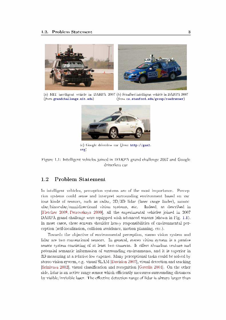
(a) MIT intelligent vehicle in DARPA 2007
(from grandchallenge.mit.edu)
(b) Stanford intelligent vehicle in DARPA 2007
(from cs.stanford.edu/group/roadrunner)
(c) Google driverless car (from http://gas2.
org)
Figure 1.1: Intelligent vehicles joined in DARPA grand challenge 2007 and Google
driverless car
1.2 Problem Statement
In intelligent vehicles, perception systems are of the most importance. Percep-
tion systems could sense and interpret surrounding environment based on var-
ious kinds of sensors, such as radar, 2D/3D lidar (laser range �nder), monoc-
ular/binocular/omnidirectional vision systems, etc. Indeed, as described in
[Fletcher 2008, Petrovskaya 2009], all the experimental vehicles joined in 2007
DARPA grand challenge were equipped with advanced sensors (shown in Fig. 1.1).
In most cases, these sensors shoulder heavy responsibilities of environmental per-
ception (self-localization, collision avoidance, motion planning, etc.).
Towards the objective of environmental perception, stereo vision system and
lidar are two conventional sensors. In general, stereo vision system is a passive
sensor system consisting of at least two cameras. It o�ers abundant texture and
potential semantic information of surrounding environments, and it is superior in
3D measuring at a relative low expense. Many perceptional tasks could be solved by
stereo vision system, e.g. visual SLAM [Davision 2007], visual detection and tracking
[Srinivasa 2002], visual classi�cation and recognition [Gavrila 2004]. On the other
side, lidar is an active range sensor which e�ciently measures surrounding distances
by visible/invisible laser. The e�ective detection range of lidar is always larger than
4 Chapter 1. Introduction
stereo vision system. Merely based on lidars, a great number of techniques are also
developed for scene perception and understanding, e.g. [Streller 2002,Cole 2006]. In
this thesis, we focus on the usages of stereo vision system and lidar.
This thesis is part of the project CPER "Intelligence du Véhicule Terrestre" (In-
telligence of ground vehicle), developed within Systems and Transportation Labora-
tory (SeT) of Institute of Research on Transportation, Energy and Society (IRTES),
UTBM, France. The problem addressed in this thesis is how to map dynamic en-
vironment by stereo vision and lidar. The main objectives and contributions are as
follows:
• The �rst objective is to estimate the ego-motion of a vehicle when it is driven.
Ego-motion estimation is a fundamental part for an intelligent vehicle. Only
by knowing the ego-motion of the vehicle itself at �rst, an intelligent vehicle
can further analyze the surrounding dynamic environment. To achieve this
objective, we implement a stereo vision based ego-motion estimation method.
Our contribution is a comparison between tracker based and matching based
circular feature associations as well as performance analysis of image feature
detectors. From the comparison, the best image feature detector and feature
association approach are selected for estimating ego-motion of the vehicle.
• The second objective is to detect and recognize independent moving objects
around the moving vehicle. This work is important for collision avoidance. We
propose a stereo vision based independent moving object detection method,
as well as a spatial information based object recognition method. The in-
dependent moving objects are detected based on the results of ego-motion
estimation, with a help of U-disparity map. The recognition is performed by
training classi�ers from spatial information of the moving objects.
• The third objective is extrinsic calibration between a stereoscopic system and
2D lidar. The extrinsic calibration between the two sensors is to calculate a
rigid 3D transformation, which connects the positions of the two sensors. We
use an ordinary chessboard to achieve the extrinsic calibration and intrinsic
calibration of the stereoscopic system at the same time. Also, we present an
optimal extrinsic calibration of the stereoscopic system and the lidar basing
on geometric constraints that use 3D planes reconstructed from stereo vision.
• The fourth objective is mapping the sensed environment by occupancy grids.
Occupancy grid map is a classic but practical tool of interpreting environ-
ment. In the thesis, we propose a stereo vision based occupancy grid mapping
method. Our contribution is about the improvement of mapping results by
analyzing the ground plane and augmenting the mapping by integrating mo-
tion and object recognition information. Then, we attempt to combine stereo
vision and lidar to improve the occupancy grid map.
1.3. Experimental Platform 5
1.3 Experimental Platform
SICK LMS 221
DSP-3000 Fiber
Optic Gyro
SICK LMS 291 Magellan Promark
RTK-GPS
Fisheye Camera
Bumblebee XB3
Stereovision System
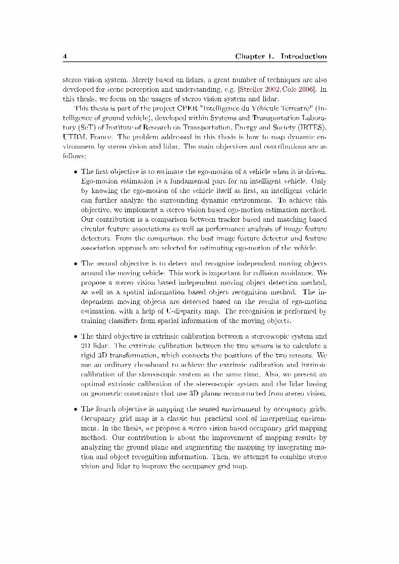
Figure 1.2: Experimental platform: SetCar developed by IRTES-SET laboratory
in UTBM
As demonstrated in Fig. 1.2, our platform SetCar is equipped by many sensors
(2D lidar, stereo vision system, �sheye camera, RTK-GPS, gyro, etc). A Bumblebee
XB3 stereo vision system is installed on the top, and oriented to the front. It contains
three collinear cameras with a maximum baseline of 240mm. Images are captured
in a format of 1280 × 960 pixels and a speed of 15 fps (frames per second). In our
application, only the left and right cameras are used. A SICK LMS 221/291 lidar
provides range measurements in a 180◦ scanning plane, with an angular resolution
of 0.5◦. It scans in 75Hz and 80 meters as maximum detective range. All of the
installed sensors are �xed rigidly.
1.4 Structure of the manuscript
In chapter 2, we review basic knowledges used in the thesis. The basic knowledges
contain the measurement models of stereo vision system and lidar, linear/nonlinear
least square methods and image feature detectors/descriptors. The reviewed basic
knowledges make understanding the thesis more easy.
6 Chapter 1. Introduction
In chapter 3, we �rst summarize a framework of stereo visual odometry. Within
the framework, di�erent kinds of feature detection and association are then com-
pared at length. From the comparison results, the best approaches of detecting and
associating image features are selected.
In chapter 4, independent moving objects are �rstly detected and segmented
based on the results of ego-motion estimation described in chapter 3. Next, spatial
information of the segmented objects are extracted based on a kernel PCA method.
Several classi�ers are learned from these spatial information for achieving indepen-
dent moving object recognition.
In chapter 5, we propose a chessboard based extrinsic calibration between a
stereoscopic system and a 2D lidar. To improve the accuracy of calibration results,
we model the sensor measurements and take the sensor models into account. We
show that by considering the sensor models, the calibration results are improved
compared with a previous method.
In chapter 6, dynamic occupancy grid map is built �rstly by stereo vision sys-
tem. It integrates motion and object recognition information. The mapping process
relies on 3D reconstruction of the stereo measures and is improved by analyzing
geometrical feature of ground plane. At the same time, occupancy grid map is also
created by lidar measures. By the extrinsic calibration results in chapter 5, we adopt
a linear opinion pool to combine the two kinds of measures to create a occupancy
grid map.
In chapter 7, conclusions and some research perspectives for this thesis are pre-
sented.
Chapter 2
Basic Knowledge
Contents
2.1 Sensor Models . . . . . . . . . . . . . . . . . . . . . . . . . . . 7
2.1.1 Coordinate Systems . . . . . . . . . . . . . . . . . . . . . . . 7
2.1.2 Lidar Measurement Model . . . . . . . . . . . . . . . . . . . . 8
2.1.3 Monocular Camera Measurement Model . . . . . . . . . . . . 9
2.1.4 Binocular Stereo Vision System Model . . . . . . . . . . . . . 13
2.2 Stereo Vision System Calibration . . . . . . . . . . . . . . . . 14
2.2.1 Intrinsic Calibration of a camera . . . . . . . . . . . . . . . . 14
2.2.2 Extrinsic Calibration of Binocular Vision System . . . . . . . 14
2.2.3 Image Undistortion and Stereo Recti�cation . . . . . . . . . . 15
2.2.4 Corner Points Triangulation . . . . . . . . . . . . . . . . . . . 17
2.3 Least Squares Estimation . . . . . . . . . . . . . . . . . . . . . 19
2.3.1 Linear Least Squares . . . . . . . . . . . . . . . . . . . . . . . 20
2.3.2 Non-linear Least Squares . . . . . . . . . . . . . . . . . . . . 25
2.3.3 Robust Estimation methods . . . . . . . . . . . . . . . . . . . 28
2.4 Image Local Feature Detectors and Descriptors . . . . . . . 30
2.4.1 Local Invariant Feature Detectors . . . . . . . . . . . . . . . . 30
2.4.2 Feature descriptors . . . . . . . . . . . . . . . . . . . . . . . . 39
2.4.3 Associating feature points through images . . . . . . . . . . . 43
2.5 Conclusion . . . . . . . . . . . . . . . . . . . . . . . . . . . . . 46
2.1 Sensor Models
As demonstrated in Fig. 1.2, our platform SetCar is equipped by many sensors (2D
lidar, stereo vision system, �sheye camera, RTK-GPS, gyro, etc). In this section, we
introduce the sensor measuring models of lidar and stereo vision system repectively.
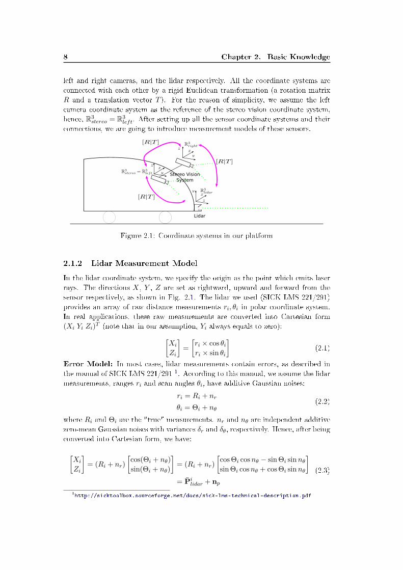
2.1.1 Coordinate Systems
To analyze such a multi-sensor system, we set several coordinate systems with re-
spect to the di�erent sensors, as demonstrated in Fig. 2.1. Let R3stereo, R
3left, R
3right,
and R3lidar, be the coordinate systems attached to the stereo vision system, the
8 Chapter 2. Basic Knowledge
left and right cameras, and the lidar respectively. All the coordinate systems are
connected with each other by a rigid Euclidean transformation (a rotation matrix
R and a translation vector T ). For the reason of simplicity, we assume the left
camera coordinate system as the reference of the stereo vision coordinate system,
hence, R3stereo = R
3left. After setting up all the sensor coordinate systems and their
connections, we are going to introduce measurement models of these sensors.
Stereo Vision
System
Lidar
Figure 2.1: Coordinate systems in our platform
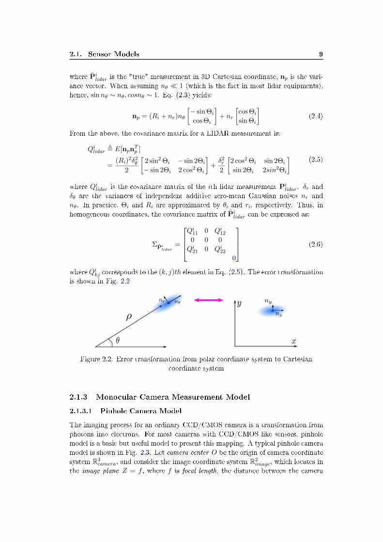
2.1.2 Lidar Measurement Model
In the lidar coordinate system, we specify the origin as the point which emits laser
rays. The directions X, Y , Z are set as rightward, upward and forward from the
sensor respectively, as shown in Fig. 2.1. The lidar we used (SICK LMS 221/291)
provides an array of raw distance measurements ri, θi in polar coordinate system.
In real applications, these raw measurements are converted into Cartesian form
(Xi Yi Zi)T (note that in our assumption, Yi always equals to zero):
[
Xi
Zi
]
=
[
ri × cos θiri × sin θi
]
(2.1)
Error Model: In most cases, lidar measurements contain errors, as described in
the manual of SICK LMS 221/291 1. According to this manual, we assume the lidar
measurements, ranges ri and scan angles θi, have additive Gaussian noises:
ri = Ri + nr
θi = Θi + nθ
(2.2)
where Ri and Θi are the "true" measurements. nr and nθ are independent additive
zero-mean Gaussian noises with variances δr and δθ, respectively. Hence, after being
converted into Cartesian form, we have:
[
Xi
Zi
]
= (Ri + nr)
[
cos(Θi + nθ)
sin(Θi + nθ)
]
= (Ri + nr)
[
cosΘi cosnθ − sinΘi sinnθ
sinΘi cosnθ + cosΘi sinnθ
]
= Pilidar + np
(2.3)
1http://sicktoolbox.sourceforge.net/docs/sick-lms-technical-description.pdf
2.1. Sensor Models 9
where Pilidar is the "true" measurement in 3D Cartesian coordinate, np is the vari-
ance vector. When assuming nθ ≪ 1 (which is the fact in most lidar equipments),
hence, sinnθ ∼ nθ, cosnθ ∼ 1. Eq. (2.3) yields:
np = (Ri + nr)nθ
[− sinΘi
cosΘi
]
+ nr
[
cosΘi
sinΘi
]
(2.4)
From the above, the covariance matrix for a LIDAR measurement is:
Qilidar ≜ E[npn
Tp ]
=(Ri)
2δ2θ2
[
2 sin2Θi − sin 2Θi
− sin 2Θi 2 cos2Θi
]
+δ2r2
[
2 cos2Θi sin 2Θi
sin 2Θi 2sin2Θi
]
(2.5)
where Qilidar is the covariance matrix of the ith lidar measurement Pi
lidar. δr and
δθ are the variances of independent additive zero-mean Gaussian noises nr and
nθ. In practice, Θi and Ri are approximated by θi and ri, respectively. Thus, in
homogeneous coordinates, the covariance matrix of Pilidar can be expressed as:
ΣPi
lidar=
Qi11 0 Qi
12
0 0 0
Qi21 0 Qi
22
0
(2.6)
whereQikj corresponds to the (k, j)th element in Eq. (2.5). The error transformation
is shown in Fig. 2.2
Figure 2.2: Error transformation from polar coordinate system to Cartesian
coordinate system
2.1.3 Monocular Camera Measurement Model
2.1.3.1 Pinhole Camera Model
The imaging process for an ordinary CCD/CMOS camera is a transformation from
photons into electrons. For most cameras with CCD/CMOS like sensors, pinhole
model is a basic but useful model to present this mapping. A typical pinhole camera
model is shown in Fig. 2.3. Let camera center O be the origin of camera coordinate
system R3camera, and consider the image coordinate system R
2image, which locates in
the image plane Z = f , where f is focal length, the distance between the camera
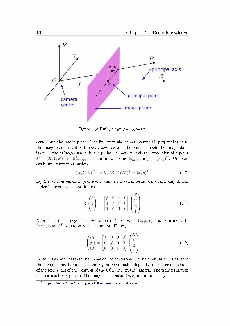
10 Chapter 2. Basic Knowledge
Figure 2.3: Pinhole camera geometry
center and the image plane. The line from the camera center O, perpendicular to
the image plane, is called the principal axis and the point it meets the image plane
is called the principal point. In the pinhole camera model, the projection of a point
P = (X,Y, Z)T in R3camera into the image plane R
2image is p = (x, y)T . One can
easily �nd their relationship:
(X,Y, Z)T 7→ (Xf/Z, Y f/Z)T = (x, y)T (2.7)
Eq. 2.7 is inconvenient in practice. It can be written in terms of matrix manipulation
under homogeneous coordinates:
Z
x
y
1
=
f 0 0 0
0 f 0 0
0 0 1 0
X
Y
Z
1
(2.8)
Note that in homogeneous coordinates 2, a point (x, y, w)T is equivalent to
(x/w, y/w, 1)T , where w is a scale factor. Hence,
x
y
1
=
f 0 0 0
0 f 0 0
0 0 1 0
X
Y
Z
1
(2.9)
In fact, the coordinates in the image do not correspond to the physical coordinates in
the image plane. For a CCD camera, the relationship depends on the size and shape
of the pixels and of the position of the CCD chip in the camera. The transformation
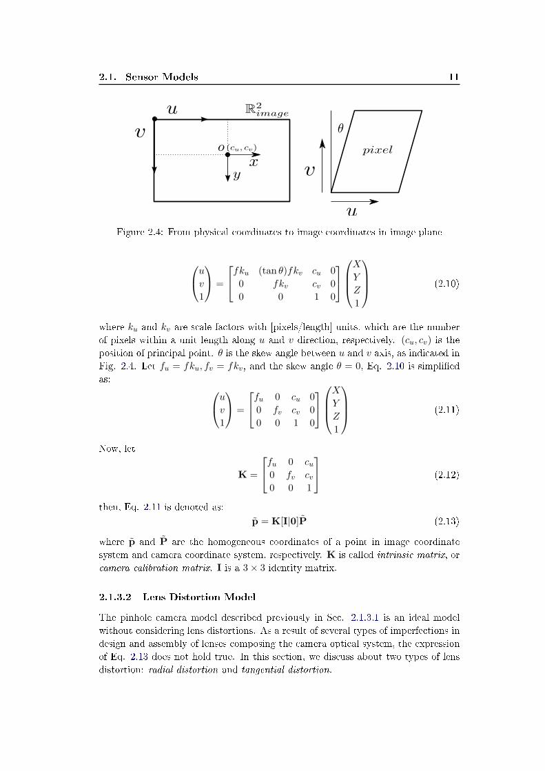
is illustrated in Fig. 2.4: The image coordinates (u, v) are obtained by:
2https://en.wikipedia.org/wiki/Homogeneous_coordinates
2.1. Sensor Models 11
Figure 2.4: From physical coordinates to image coordinates in image plane
u
v
1
=
fku (tan θ)fkv cu 0
0 fkv cv 0
0 0 1 0
X
Y
Z
1
(2.10)
where ku and kv are scale factors with [pixels/length] units, which are the number
of pixels within a unit length along u and v direction, respectively. (cu, cv) is the
position of principal point. θ is the skew angle between u and v axis, as indicated in
Fig. 2.4. Let fu = fku, fv = fkv, and the skew angle θ = 0, Eq. 2.10 is simpli�ed
as:
u
v
1
=
fu 0 cu 0
0 fv cv 0
0 0 1 0
X
Y
Z
1
(2.11)
Now, let
K =
fu 0 cu0 fv cv0 0 1
(2.12)
then, Eq. 2.11 is denoted as:
p = K[I|0]P (2.13)
where p and P are the homogeneous coordinates of a point in image coordinate
system and camera coordinate system, respectively. K is called intrinsic matrix, or
camera calibration matrix. I is a 3× 3 identity matrix.
2.1.3.2 Lens Distortion Model
The pinhole camera model described previously in Sec. 2.1.3.1 is an ideal model
without considering lens distortions. As a result of several types of imperfections in
design and assembly of lenses composing the camera optical system, the expression
of Eq. 2.13 does not hold true. In this section, we discuss about two types of lens
distortion: radial distortion and tangential distortion.

12 Chapter 2. Basic Knowledge
(a) Reason of radial distortions
Ideal
Position
Position with
Distortion
: radial distortion
: Tangential distortion
(b) Radial and tangential distortions
Figure 2.5: lens distortions
• Radial distortion: This type of distortion is mainly caused by physical
�awed lens geometry, which makes the input and output ray have di�erent
angle, as shown in Fig. 2.5 (a). It results in an inward or outward shift of
image points from their initial perspective projection, as denoted in dr in Fig.
2.5 (b).
• Tangential distortion: This type of distortion is caused by errors in optical
component shapes and optics assembly. It is also called decentering distortion.
It is illustrated in Fig. 2.5 (b) as dt.
Let a point (xd, yd) be the distorted coordinates of a point (x, y) in image plane
coordinate system R2image, and r2 = x2 + y2. Then:
(
xdyd
)
= (1 + k1r2 + k2r
4 + k3r6) ·
(
x
y
)
+ dt (2.14)
where k1, k2, k3 are the coe�cients of radial distortion. dt is the tangential distortion
vector:
dt =
[
2p1xy + p2(r2 + 2x2)
p1(r2 + 2y2) + 2p2xy
]
(2.15)
where p1, p2 are the coe�cients of tangential distortion. Therefore, under the lens
distortion model, the pixel coordinates (u, v) are related to distorted coordinates
similar to Eq. 2.13:
u
v
1
= K
xdyd1
(2.16)
where (xd, yd) is represented in Eq. 2.14.

2.1. Sensor Models 13
2.1.4 Binocular Stereo Vision System Model
As an extension of monocular camera model, a general binocular stereo vision model
is shown in Fig. 2.6 The left and right cameras are modeled by the classical pinhole
Epipolar plane
Epipolar
line
Epipole
Figure 2.6: Geometry of binocular stereo vision system
model, with intrinsic matrices Kl and Kr respectively. Therefore, suppose there is
a point P in 3D space, its corresponding coordinates in the left camera coordinate
system R3left, the right camera coordinate system R
3right, the left image coordinate
system R2left and the right image coordinate system R
2right are Pl, Pr, pl, pr respec-
tively. Then, they are connected as:
pl = Kl[I|0] · Pl
pr = Kr[I|0] · Pr
Pl = Rlr · Pr +Tl
r
(2.17)
where · denotes homogeneous coordinates. Rlr, (a 3 × 3 rotation matrix) together
withTrr (a 3×1 translation vector) represent rigid 3D Euclidean transformation from
R3right to R
3left. In similar, Rr
l and Trl describe a rigid 3D Euclidean transformation
from R3left to R
3right. Usually, R and T are called extrinsic parameters.
Another characteristic of binocular vision system is the epipolar geometry. In
epipolar geometry, the point intersections of the base line OlOr with the two image
planes are epipoles. Any point P in 3D space with two camera centers Ol and Or
de�ne an epipolar plane. The line intersections of the epipolar plane with the two
image planes are called epipolar lines. Indeed, all epipolar lines intersect at epipole.
An epipolar plane de�nes the correspondence between the epipolar lines. All the
epipoles, epipolar plane and epipolar lines are drawn in Fig. 2.6. Based on the
above de�nitions, epipolar constraint is that: suppose pl is the left image position

14 Chapter 2. Basic Knowledge
for a scene point P , then, the corresponding point pr in the right image must lie
on the epipolar line. The mathematical interpretation is that, for a corresponding
point pair (pl, pr) in homogeneous coordinates ·, we have:
pTl F pr = 0 (2.18)
where F is called fundamental matrix. F pr describes a line (an epipolar line) on
which the corresponding point pl must lie.
2.2 Stereo Vision System Calibration
2.2.1 Intrinsic Calibration of a camera
Intrinsic calibration of a camera is to �nd the intrinsic parameters described in Sec.
2.1.3 (focal length, principal point position, as well as lens distortion). It is essential
in 3D computer vision, such as 3D Euclidean structure from motion, object avoid-
ance in robot navigation, etc.. A calibrated camera can be used as a quantitative
sensor being capable of measuring distance and 3D structure information.
Intrinsic calibration of a camera has been researched for decades. Among all
the proposed methods, 2D planer pattern based methods, e.g. Zhengyou Zhang's
method [Zhang 2000], is the most popular. This method requires the camera to
observe a planar pattern (e.g. 2D chessboard) shown at a few di�erent orientations.
Either the camera or the planar pattern can be freely moved. It is implemented
in a well known camera calibration toolbox for Matlab 3, developed by Jean-Yves
Bouguet [Bouguet 1999]. This Matlab calibration toolbox is applied in our practices.
The whole process is as follows:
• Prepare a chessboard pattern and attach it to a planar surface.
• Take a few images of the chessboard under di�erent positions with di�erent
orientations, as shown in Fig. 2.7 (a).
• Detect the corner points on the chessboard images, as shown in Fig. 2.7 (b).
• Estimate the intrinsic parameters and the coe�cients of radial distortion
through a nonlinear optimization process. The calibration results and error
analysis are shown in Fig. 2.7.
2.2.2 Extrinsic Calibration of Binocular Vision System
Extrinsic calibration of a stereo rig is to estimate extrinsic parameters between left
and right cameras (a rotation matrix and a translation vector, as described in Sec.
2.1.4). Given corresponding image points from two views, the extrinsic parameters
can be calculated from SVD factorizing the fundamental matrix F [Hartley 2004].
3http://www.vision.caltech.edu/bouguetj/calib_doc/
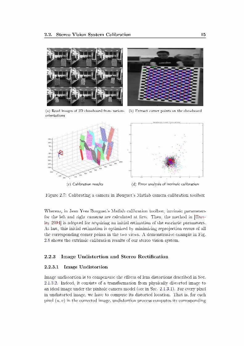
2.2. Stereo Vision System Calibration 15
(a) Read images of 2D chessboard from various
orientations
(b) Extract corner points on the chessboard
(c) Calibration results (d) Error analysis of intrinsic calibration
Figure 2.7: Calibrating a camera in Bouguet's Matlab camera calibration toolbox
Whereas, in Jean-Yves Bouguet's Matlab calibration toolbox, intrinsic parameters
for the left and right cameras are calculated at �rst. Then, the method in [Hart-
ley 2004] is adopted for acquiring an initial estimation of the extrinsic parameters.
At last, this initial estimation is optimized by minimizing reprojection errors of all
the corresponding corner points in the two views. A demonstrative example in Fig.
2.8 shows the extrinsic calibration results of our stereo vision system.
2.2.3 Image Undistortion and Stereo Recti�cation
2.2.3.1 Image Undistortion
Image undistortion is to compensate the e�ects of lens distortions described in Sec.
2.1.3.2. Indeed, it consists of a transformation from physically distorted image to
an ideal image under the pinhole camera model (see in Sec. 2.1.3.1). For every pixel
in undistorted image, we have to compute its distorted location. That is, for each
pixel (u, v) in the corrected image, undistortion process computes its corresponding
16 Chapter 2. Basic Knowledge
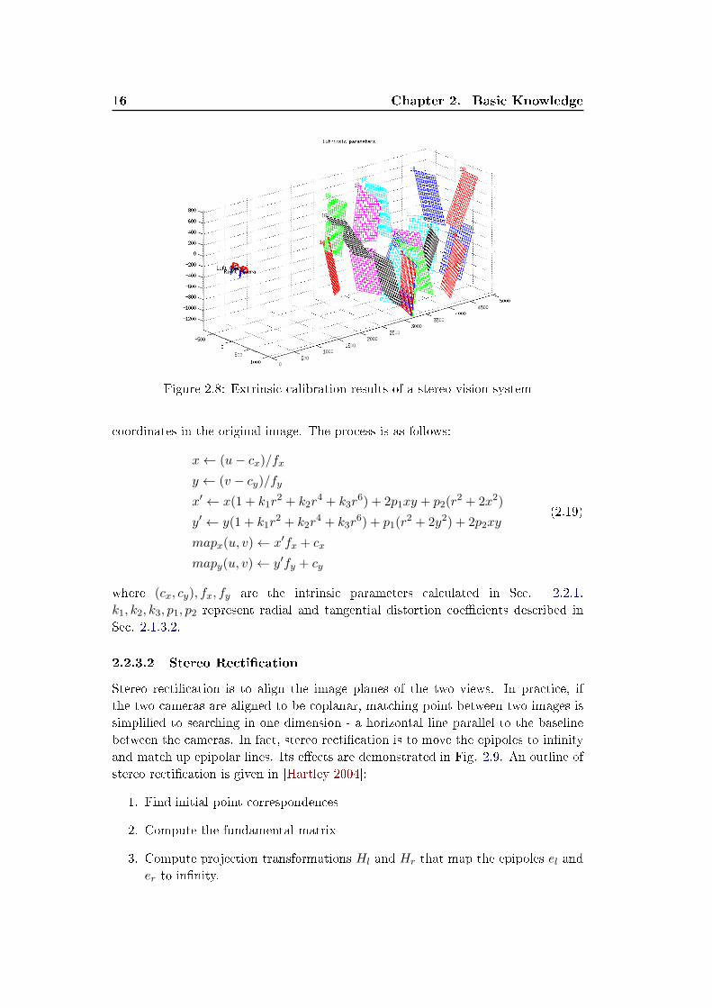
Figure 2.8: Extrinsic calibration results of a stereo vision system
coordinates in the original image. The process is as follows:
x← (u− cx)/fx
y ← (v − cy)/fy
x′ ← x(1 + k1r2 + k2r
4 + k3r6) + 2p1xy + p2(r
2 + 2x2)
y′ ← y(1 + k1r2 + k2r
4 + k3r6) + p1(r
2 + 2y2) + 2p2xy
mapx(u, v)← x′fx + cx
mapy(u, v)← y′fy + cy
(2.19)
where (cx, cy), fx, fy are the intrinsic parameters calculated in Sec. 2.2.1.
k1, k2, k3, p1, p2 represent radial and tangential distortion coe�cients described in
Sec. 2.1.3.2.
2.2.3.2 Stereo Recti�cation
Stereo recti�cation is to align the image planes of the two views. In practice, if
the two cameras are aligned to be coplanar, matching point between two images is
simpli�ed to searching in one dimension - a horizontal line parallel to the baseline
between the cameras. In fact, stereo recti�cation is to move the epipoles to in�nity
and match up epipolar lines. Its e�ects are demonstrated in Fig. 2.9. An outline of
stereo recti�cation is given in [Hartley 2004]:
1. Find initial point correspondences
2. Compute the fundamental matrix
3. Compute projection transformations Hl and Hr that map the epipoles el and
er to in�nity.
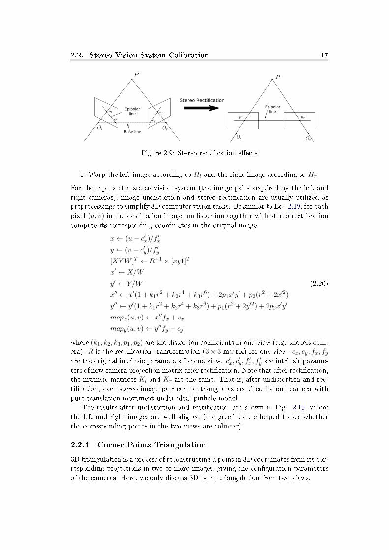
2.2. Stereo Vision System Calibration 17
Epipolar
line
Base line
Epipolar
line
Stereo Rectification
Figure 2.9: Stereo recti�cation e�ects
4. Warp the left image according to Hl and the right image according to Hr
For the inputs of a stereo vision system (the image pairs acquired by the left and
right cameras), image undistortion and stereo recti�cation are usually utilized as
preprocessings to simplify 3D computer vision tasks. Be similar to Eq. 2.19, for each
pixel (u, v) in the destination image, undistortion together with stereo recti�cation
compute its corresponding coordinates in the original image:
x← (u− c′x)/f′x
y ← (v − c′y)/f′y
[XYW ]T ← R−1 × [xy1]T
x′ ← X/W
y′ ← Y/W
x′′ ← x′(1 + k1r2 + k2r
4 + k3r6) + 2p1x
′y′ + p2(r2 + 2x′2)
y′′ ← y′(1 + k1r2 + k2r
4 + k3r6) + p1(r
2 + 2y′2) + 2p2x′y′
mapx(u, v)← x′′fx + cx
mapy(u, v)← y′′fy + cy
(2.20)
where (k1, k2, k3, p1, p2) are the distortion coe�cients in one view (e.g. the left cam-
era). R is the recti�cation transformation (3× 3 matrix) for one view. cx, cy, fx, fyare the original intrinsic parameters for one view. c′x, c
′y, f
′x, f
′y are intrinsic parame-
ters of new camera projection matrix after recti�cation. Note that after recti�cation,
the intrinsic matrices Kl and Kr are the same. That is, after undistortion and rec-
ti�cation, each stereo image pair can be thought as acquired by one camera with
pure translation movement under ideal pinhole model.
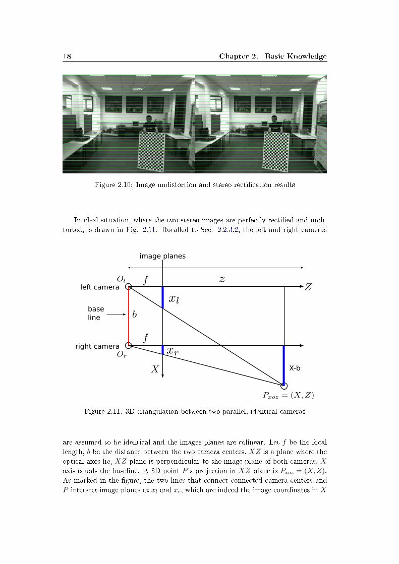
The results after undistortion and recti�cation are shown in Fig. 2.10, where
the left and right images are well aligned (the greelines are helped to see whether
the corresponding points in the two views are colinear).
2.2.4 Corner Points Triangulation
3D triangulation is a process of reconstructing a point in 3D coordinates from its cor-
responding projections in two or more images, giving the con�guration parameters
of the cameras. Here, we only discuss 3D point triangulation from two views.
18 Chapter 2. Basic Knowledge
Figure 2.10: Image undistortion and stereo recti�cation results
In ideal situation, where the two stereo images are perfectly recti�ed and undi-
torted, is drawn in Fig. 2.11. Recalled to Sec. 2.2.3.2, the left and right cameras
base
line
left camera
right camera
image planes
X-b
Figure 2.11: 3D triangulation between two parallel, identical cameras
are assumed to be identical and the images planes are colinear. Let f be the focal
length, b be the distance between the two camera centers, XZ is a plane where the
optical axes lie, XZ plane is perpendicular to the image plane of both cameras, X
axis equals the baseline. A 3D point P 's projection in XZ plane is Pxoz = (X,Z).
As marked in the �gure, the two lines that connect connected camera centers and
P intersect image planes at xl and xr, which are indeed the image coordinates in X
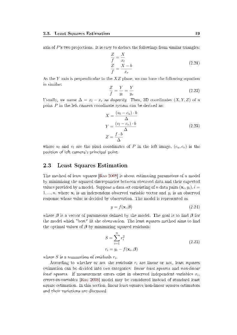
2.3. Least Squares Estimation 19
axis of P 's two projections. It is easy to deduct the followings from similar triangles:
Z
f=
X
xlZ
f=
X − b
xr
(2.21)
As the Y -axis is perpendicular to the XZ plane, we can have the following equation
in similar:Z
f=
Y
yl=
Y
yr(2.22)
Usually, we name ∆ = xl − xr as disparity. Then, 3D coordinates (X,Y, Z) of a
point P in the left camera coordinate system can be derived as:
X =(ul − cu) · b
∆
Y =(vl − cv) · b
∆
Z =f · b∆
(2.23)
where ul and vl are the pixel coordinates of P in the left image, (cu, cv) is the
position of left camera's principal point.
2.3 Least Squares Estimation
The method of least squares [Rao 2008] is about estimating parameters of a model
by minimizing the squared discrepancies between observed data and their expected
values provided by a model. Suppose a data set consisting of n data pairs (xi, yi), i =
1, ..., n, where xi is an independent observed variable vector and yi is an observed
response whose value is decided by observation. The model is represented as
y = f(x,β) (2.24)
where β is a vector of parameters de�ned by the model. The goal is to �nd β for
the model which "best" �t the observation. The least squares method aims to �nd
the optimal values of β by minimizing squared residuals:
S =n∑
i=1
r2i
ri = yi − f(xi,β)
(2.25)
where S is a summation of residuals ri.
According to whether or not the residuals ri are linear or not, least squares
estimation can be divided into two categories: linear least squares and non-linear
least squares. If measurement errors exist in observed independent variables xi,
errors-in-variables [Rao 2008] model may be considered instead of standard least
square estimation. In this section, linear least squares/non-linear squares estimators
and their variations are discussed.
20 Chapter 2. Basic Knowledge
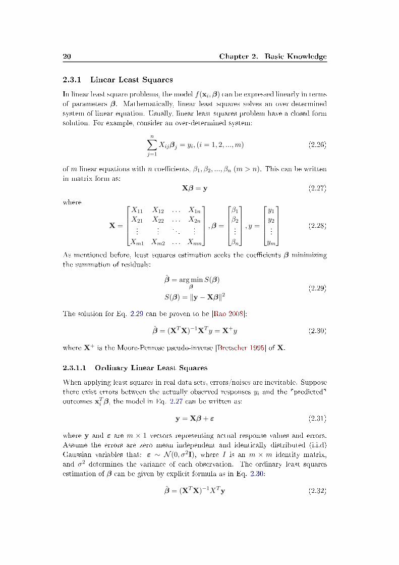
2.3.1 Linear Least Squares
In linear least square problems, the model f(xi,β) can be expressed linearly in terms
of parameters β. Mathematically, linear least squares solves an over-determined
system of linear equation. Usually, linear least squares problem have a closed-form
solution. For example, consider an over-determined system:
n∑
j=1
Xijβj = yi, (i = 1, 2, ...,m) (2.26)
of m linear equations with n coe�cients, β1, β2, ..., βn (m > n). This can be written
in matrix form as:
Xβ = y (2.27)
where
X =
X11 X12 . . . X1n
X21 X22 . . . X2n...
.... . .
...
Xm1 Xm2 . . . Xmn
,β =
β1β2...
βn
, y =
y1y2...
ym
(2.28)
As mentioned before, least squares estimation seeks the coe�cients β minimizing
the summation of residuals:
β = argminβ
S(β)
S(β) = ∥y −Xβ∥2(2.29)
The solution for Eq. 2.29 can be proven to be [Rao 2008]:
β = (XTX)−1XT y = X+y (2.30)
where X+ is the Moore-Penrose pseudo-inverse [Bretscher 1995] of X.
2.3.1.1 Ordinary Linear Least Squares
When applying least squares in real data sets, errors/noises are inevitable. Suppose
there exist errors between the actually observed responses yi and the "predicted"
outcomes xTi β, the model in Eq. 2.27 can be written as:
y = Xβ + ε (2.31)
where y and ε are m × 1 vectors representing actual response values and errors.
Assume the errors are zero mean independent and identically distributed (i.i.d)
Gaussian variables that: ε ∼ N (0, σ2I), where I is an m × m identity matrix,
and σ2 determines the variance of each observation. The ordinary least squares
estimation of β can be given by explicit formula as in Eq. 2.30:
β = (XTX)−1XTy (2.32)
2.3. Least Squares Estimation 21
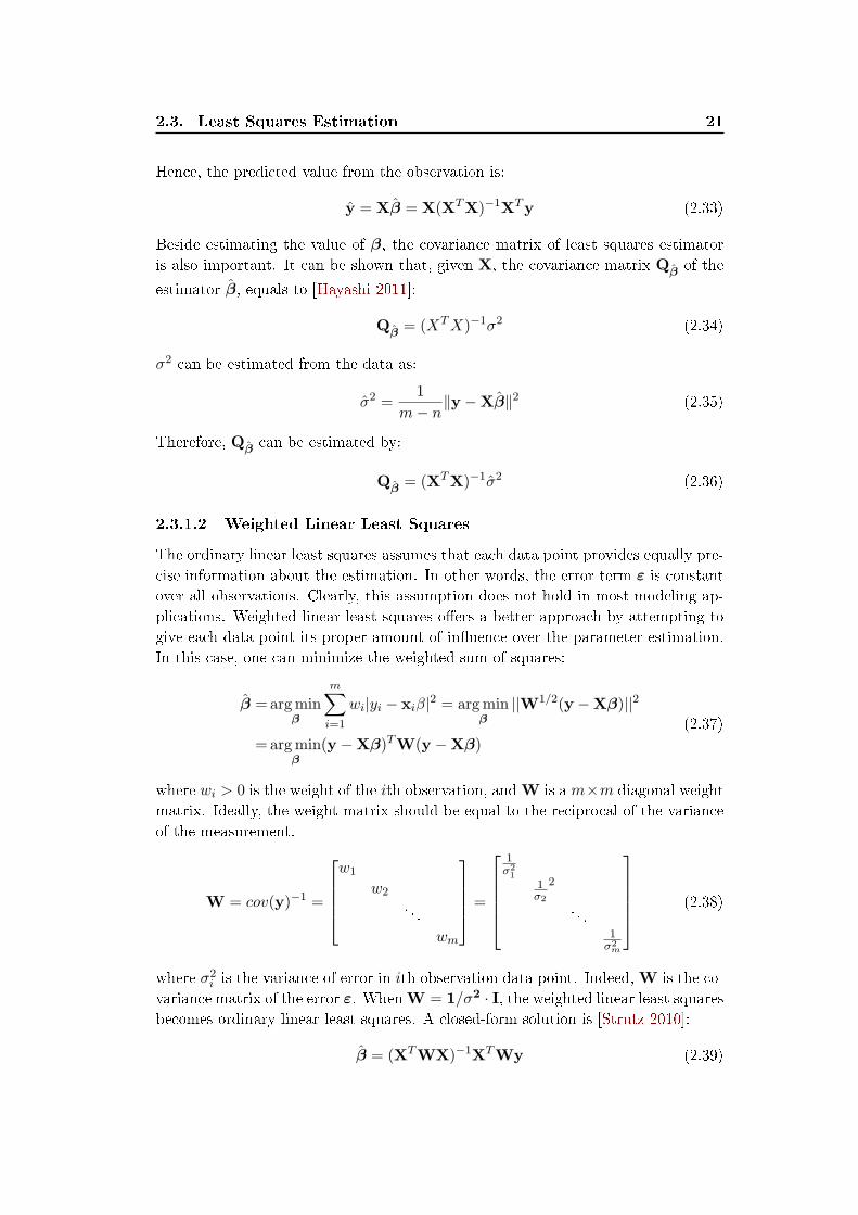
Hence, the predicted value from the observation is:
y = Xβ = X(XTX)−1XTy (2.33)
Beside estimating the value of β, the covariance matrix of least squares estimator
is also important. It can be shown that, given X, the covariance matrix Qβof the
estimator β, equals to [Hayashi 2011]:
Qβ= (XTX)−1σ2 (2.34)
σ2 can be estimated from the data as:
σ2 =1
m− n∥y −Xβ∥2 (2.35)
Therefore, Qβcan be estimated by:
Qβ= (XTX)−1σ2 (2.36)
2.3.1.2 Weighted Linear Least Squares
The ordinary linear least squares assumes that each data point provides equally pre-
cise information about the estimation. In other words, the error term ε is constant
over all observations. Clearly, this assumption does not hold in most modeling ap-
plications. Weighted linear least squares o�ers a better approach by attempting to
give each data point its proper amount of in�uence over the parameter estimation.
In this case, one can minimize the weighted sum of squares:
β =argminβ
m∑
i=1
wi|yi − xiβ|2 = argminβ
||W1/2(y −Xβ)||2
=argminβ
(y −Xβ)TW(y −Xβ)
(2.37)
where wi > 0 is the weight of the ith observation, and W is a m×m diagonal weight
matrix. Ideally, the weight matrix should be equal to the reciprocal of the variance
of the measurement.
W = cov(y)−1 =
w1
w2
. . .
wm
=
1σ21
1σ2
2
. . .1σ2m
(2.38)
where σ2i is the variance of error in ith observation data point. Indeed, W is the co-
variance matrix of the error ε. WhenW = 1/σ2 · I, the weighted linear least squares
becomes ordinary linear least squares. A closed-form solution is [Strutz 2010]:
β = (XTWX)−1XTWy (2.39)
22 Chapter 2. Basic Knowledge
The covariance matrix Qβof estimation β, can be acquired by applying error prop-
agation law:
Qβ= (XTWX)−1XTWX(XTWX)−1 (2.40)
However, in many real practices, we do not know σ2i . We could set the weights
manually or by an iterative approach: iteratively reweighted least squares (IRLS)
[Chartrand 2008]. IRLS uses an iterative approach to solve a weighted least squares
problem of the form:
β(t+1)
= argminβ
m∑
i=1
wi|yi − xiβi|2 (2.41)
In each step t+1, the IRLS estimates β(t+1)
by the aforementioned weighted linear
least squares:
β(t+1)
= (XTW(t)X)−1XTW(t)y (2.42)
where W(t) is a diagonal weight matrix in tth step with each element:
w(t)i = |yi − xiβ
(t)|−1 (2.43)
2.3.1.3 Total Linear Least Squares
The above ordinary and weighted linear least squares only assume errors in the
observed response y, as interpreted in Eq. 2.31. However, it is a more natural way
to model data if both observation X and response y are contaminated by errors.
Total least squares (TLS) [Hu�el 1991], is a natural generalization of ordinary least
squares where errors in all observational variables are taken into account.
TLS problem is de�ned as follows: we are given an over-determined set of m
equations xiβ = yi (i = 1...m) in n unknowns βj(j = 1...n), compiled to a matrix
equation Xβ ≈ y. Both the vector y as well as the matrix X are subject to errors.
The total least squares problem consists in �nding an m×n matrix X and an m×1
vector y for which the equation
Xβ = y (2.44)
has an exact solution, under the condition that the deviation between (X|y) and
(X|y) is minimal in terms of the Frobenius norm:
min ∥(X|y)− (X|y)∥F (2.45)
For a m × n matrix A = (ai,j) i = 1...m, j = 1...n, the Frobenius norm is de�ned
as:
∥A∥F =
√
√
√
√
m∑
i=1
n∑
j=1
|aij |2 =√
trace(A∗A) =
√
√
√
√
min(m,n)∑
i=1
σ2i (2.46)
where A∗ denotes the conjugate transpose, σi are the singular values of A. Further-
more, we denote the errors lying in X and y as E (m × n matrix) and r (m × 1
vector), respectively. The TLS model becomes:
(X+E)β = (y + r) (2.47)
2.3. Least Squares Estimation 23
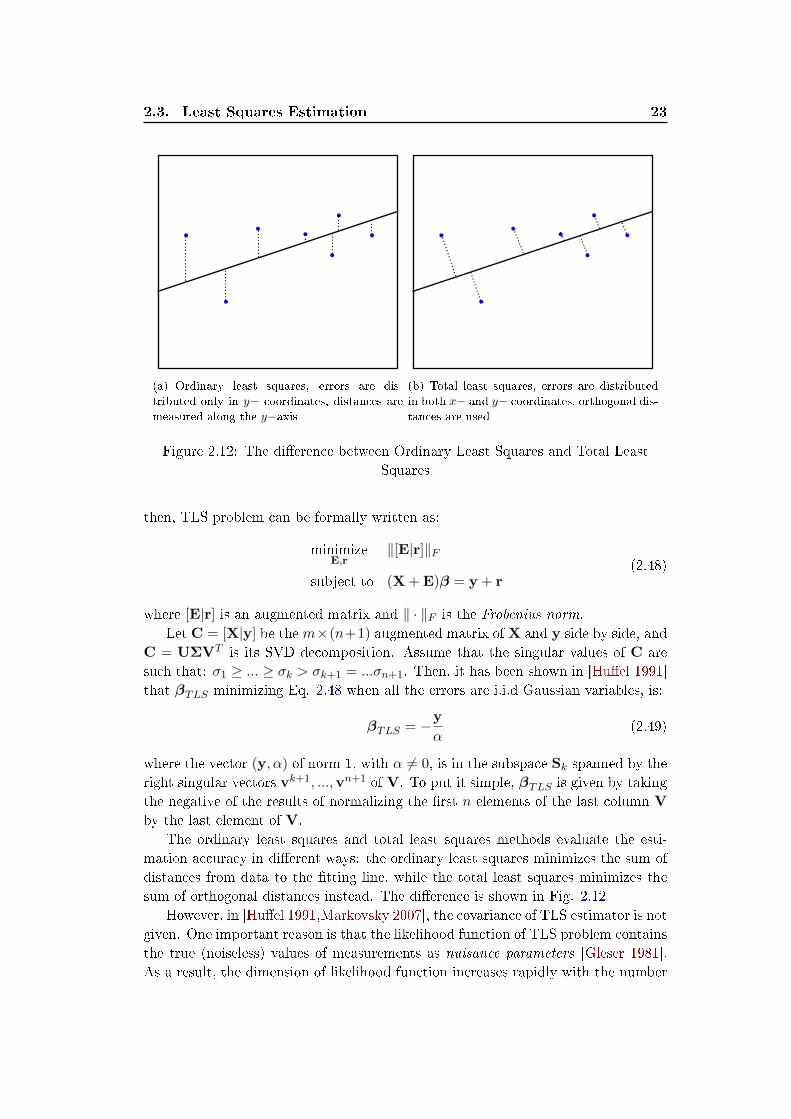
(a) Ordinary least squares, errors are dis-
tributed only in y− coordinates, distances are
measured along the y−axis
(b) Total least squares, errors are distributed
in both x− and y− coordinates, orthogonal dis-
tances are used
Figure 2.12: The di�erence between Ordinary Least Squares and Total Least
Squares
then, TLS problem can be formally written as:
minimizeE,r
∥[E|r]∥F
subject to (X+E)β = y + r(2.48)
where [E|r] is an augmented matrix and ∥ · ∥F is the Frobenius norm.
Let C = [X|y] be the m×(n+1) augmented matrix of X and y side by side, and
C = UΣVT is its SVD decomposition. Assume that the singular values of C are
such that: σ1 ≥ ... ≥ σk > σk+1 = ...σn+1. Then, it has been shown in [Hu�el 1991]
that βTLS minimizing Eq. 2.48 when all the errors are i.i.d Gaussian variables, is:
βTLS = −y
α(2.49)
where the vector (y, α) of norm 1, with α = 0, is in the subspace Sk spanned by the
right singular vectors vk+1, ...,vn+1 of V. To put it simple, βTLS is given by taking
the negative of the results of normalizing the �rst n elements of the last column V
by the last element of V.
The ordinary least squares and total least squares methods evaluate the esti-
mation accuracy in di�erent ways: the ordinary least squares minimizes the sum of
distances from data to the �tting line, while the total least squares minimizes the
sum of orthogonal distances instead. The di�erence is shown in Fig. 2.12
However, in [Hu�el 1991,Markovsky 2007], the covariance of TLS estimator is not
given. One important reason is that the likelihood function of TLS problem contains
the true (noiseless) values of measurements as nuisance parameters [Gleser 1981].
As a result, the dimension of likelihood function increases rapidly with the number

24 Chapter 2. Basic Knowledge
of observations. In [Nestares 2000], the likelihood function of TLS is simpli�ed with
several assumptions and the Cramer-Rao lower bound (CRLB) 4 of TLS is given:
Q(β)TLS≥ CRLB(βTLS) =
1
γσ2n∥(β)TLS∥2(XTX)−1 (2.50)
where σn is the variance of the assuming i.i.d distributed measurement noises. γ =σ20
σ2n+σ2
0is related with the signal to noise ratio (SNR). If the SNR is high (σ2
0 ≫ σ2n),
then γ ≈ 1.
4http://en.wikipedia.org/wiki/Cramer-Rao_bound
2.3. Least Squares Estimation 25
2.3.2 Non-linear Least Squares
Be di�erent to the linear least squares introduced in Sec. 2.3.1, the observation
model f(x,β) (in Eq. 2.24) in non-linear least squares can not be represented in
form of linear combination of parameters β = βi(i = 1...n). Solutions of non-
linear least squares usually approximate non-linear model by a linear one, and re-
�ne the parameter vector β iteratively. Recall to Eq. 2.24, given m data points
(x1,y1), (x2,y2), ..., (xm,ym) and a non-linear model y = f(x,β), with m ⩾ n.
Non-linear least squares is to �nd the parameter vector β, which minimizes the sum
of squares:
S =
m∑
i=1
r2i (2.51)
where the residuals ri are given by:
ri = yi − f(xi,β), i = 1, 2, ...,m (2.52)
According to the knowledge of calculus, the sum of squares S reaches a minimum
when the gradient is zero. Since the model contains n parameters, there are n
gradient equations:
∂S
∂βj= 2
∑
i
ri∂ri∂βj
= 0 (j = 1, ..., n) (2.53)
For a non-linear model, the partial derivatives ∂ri∂βj
are in terms of desired parameters
as well as independent variables. Hence, it is usually impossible to get a closed so-
lution. Instead, iterative methods are widely chosen to approximate optimal results
in successive manners:
βj ≈ βk+1j = βk
j +∆βj (2.54)
where k denotes the kth round of iteration. ∆β is known as the shift vector. In each
step of iteration, the model f(x,β) can be linearly approximated by a �rst-order
Taylor series expansion at βk:
f(xi,β) ≈ f(xi,βk) +
∑
j
∂f(xi,βk)
∂βj(βj − βk
j ) ≈ f(xi,βk) +
∑
j
Jij∆βj (2.55)
where Jij is the (i, j)th element of Jacobian matrix 5 J.
J =
∂f(x1,βk)/∂β1 · · · ∂f(x1,β
k)/∂βn...
. . ....
∂f(xm,βk)/∂β1 · · · ∂f(xm,βk)/βn
(2.56)
Therefore, Jij = − ∂ri∂βj
. and the residuals in Eq. 2.52 are represented as:
ri =yi − (f(xi, βk) +
∑
j
Jij∆βj)
=∆yi −n∑
j=1
Jij∆βj
(2.57)
5https://en.wikipedia.org/wiki/Jacobian_matrix
26 Chapter 2. Basic Knowledge
Substituting Eq. 2.57 into Eq. 2.53, and rearranging the equations in terms of
matrix, we have:
(JTJ)∆β = JT∆y (2.58)
This equation forms the basis for many other iterative approaches of non-linear least
squares problem.
2.3.2.1 Gauss-Newton Algorithm
Gauss-Newton algorithm (GNA) [Bjorck 1996] is very popular to solve non-linear
least squares problems. Its biggest advantage is to avoid computing second deriva-
tives.
According to Eq. 2.58, the shift vector for each iteration step can be solved by
linear least squares as in Eq. 2.32
∆β = (JTJ)−1JT∆y (2.59)
Then, in each iteration step, estimated parameters are updated as:
βk+1 = βk + (JTJ)−1JT r(βk) (2.60)
where the residual r(βk) is expressed as:
r(βk) = y − f(x,βk) (2.61)
In summary, given an initial guess of β0 at the beginning, Gauss-Newton algo-
rithm iteratively updates the required parameters as in Eq. 2.60 until r(βk) closes
to zero or ∆βk is tiny.
2.3.2.2 Levenberg-Marquardt Algorithm
Levenberg-Marquardt algorithm (LMA) [Levenberg 1944,Marquardt 1963] provides
a more robust solution of non-linear least squares than Gauss-Newton algorithm
(GNA). In many cases, it converges to local minimum, even if the initial guess
starts very far from the �nal minimum.
Like Gauss-Newton algorithm, Levenberg-Marquardt algorithm is also an iter-
ative method. Recall to Eq. 2.58, which is the basis of Gauss-Newton algorithm.
Levenberg [Levenberg 1944] �rstly replace this equation by a "damped version":
(JTJ+ λI)∆β = JT∆y (2.62)
where I is the identity matrix. λ is a non-negative damping factor, which is adjusted
at each iteration. If the S in Eq. 2.51 reduces rapidly, a small value of λ can be used,
making the algorithm closer to Gauss-Newton algorithm. Whereas, if an iteration
causes insu�cient reduction of the residual, λ can be increased, giving a step closer
to the gradient descent direction (note that the gradient of S with respect to β
equals −2(JT∆y)). Levenberg's algorithm has the disadvantage that if the value
2.3. Least Squares Estimation 27
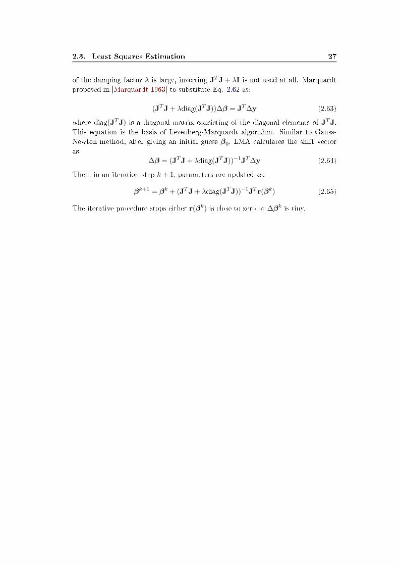
of the damping factor λ is large, inverting JTJ + λI is not used at all. Marquardt
proposed in [Marquardt 1963] to substitute Eq. 2.62 as:
(JTJ+ λdiag(JTJ))∆β = JT∆y (2.63)
where diag(JTJ) is a diagonal matrix consisting of the diagonal elements of JTJ.
This equation is the basis of Levenberg-Marquardt algorithm. Similar to Gauss-
Newton method, after giving an initial guess β0, LMA calculates the shift vector
as:
∆β = (JTJ+ λdiag(JTJ))−1JT∆y (2.64)
Then, in an iteration step k + 1, parameters are updated as:
βk+1 = βk + (JTJ+ λdiag(JTJ))−1JT r(βk) (2.65)
The iterative procedure stops either r(βk) is close to zero or ∆βk is tiny.
28 Chapter 2. Basic Knowledge
2.3.3 Robust Estimation methods
Robust estimation methods, or robust statistical methods, is designed to deal with
outliers in data. Another motivation is to provide methods with good perfor-
mance when there is a mixture of models. From statistical theory, M-estimator
or least-median squares [Godambe 1991] are proposed. While here, we only de-
scribe RANSAC algorithm, a widely used robust estimation method developed from
computer vision community.
2.3.3.1 RANSAC algorithm
RANSAC (RANdom SAmple Consensus) [Fischler 1981] is a general parameter esti-
mation approach designed to cope with a large proportion of outliers in input data.
It is also a non-deterministic algorithm, which means that it gives a reasonable result
by a certain probability.
In aforementioned least squares methods, all the observational data are assumed
to be as inliers � data �t the model only subject to noise at some extent. However,
outliers, data do not �t the model at all, are pervasive in real applications. The out-
liers maybe come from extreme values of noise, erroneous measurements, incorrect
hypotheses about the interpretation of data, etc.
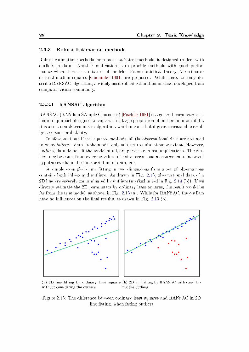
A simple example is line �tting in two dimensions from a set of observations
contains both inliers and outliers. As drawn in Fig. 2.13, observational data of a
2D line are severely contaminated by outliers (marked in red in Fig. 2.13 (b)). If we
directly estimate the 2D parameters by ordinary least squares, the result would be
far from the true model, as shown in Fig. 2.13 (a). While for RANSAC, the outliers
have no in�uences on the �nal results, as drawn in Fig. 2.13 (b).
(a) 2D line �tting by ordinary least squares
without considering the outliers
(b) 2D line �tting by RANSAC with consider-
ing the outliers
Figure 2.13: The di�erence between ordinary least squares and RANSAC in 2D
line �tting, when facing outliers
2.3. Least Squares Estimation 29
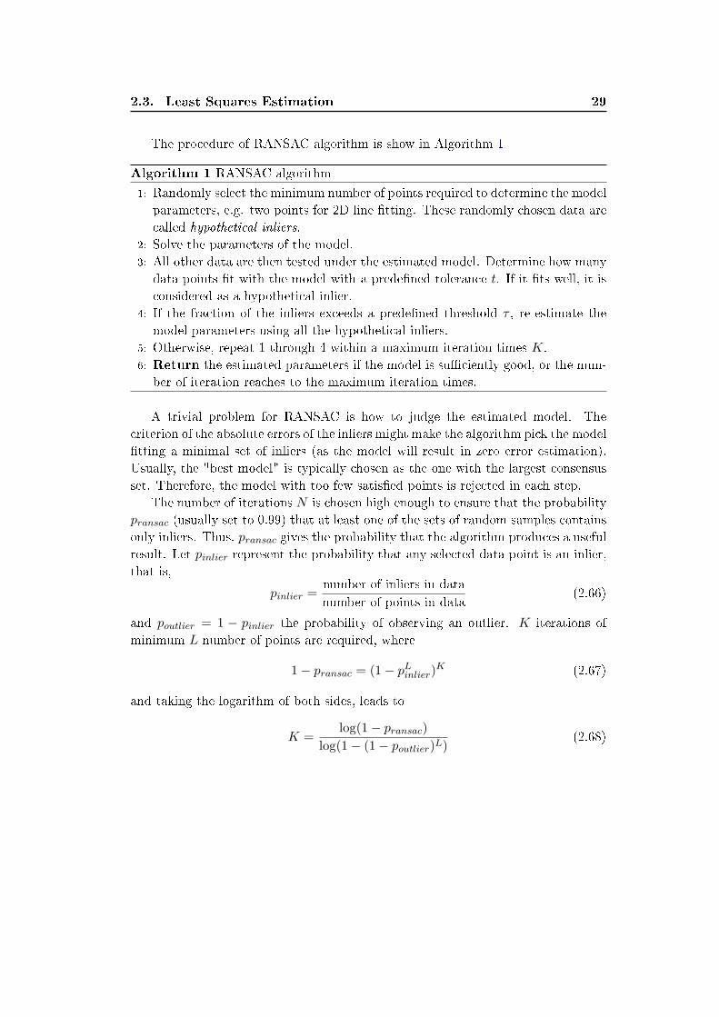
The procedure of RANSAC algorithm is show in Algorithm 1
Algorithm 1 RANSAC algorithm
1: Randomly select the minimum number of points required to determine the model
parameters, e.g. two points for 2D line �tting. These randomly chosen data are
called hypothetical inliers.
2: Solve the parameters of the model.
3: All other data are then tested under the estimated model. Determine how many
data points �t with the model with a prede�ned tolerance t. If it �ts well, it is
considered as a hypothetical inlier.
4: If the fraction of the inliers exceeds a prede�ned threshold τ , re-estimate the
model parameters using all the hypothetical inliers.
5: Otherwise, repeat 1 through 4 within a maximum iteration times K.
6: Return the estimated parameters if the model is su�ciently good, or the num-
ber of iteration reaches to the maximum iteration times.
A trivial problem for RANSAC is how to judge the estimated model. The
criterion of the absolute errors of the inliers might make the algorithm pick the model
�tting a minimal set of inliers (as the model will result in zero error estimation).
Usually, the "best model" is typically chosen as the one with the largest consensus
set. Therefore, the model with too few satis�ed points is rejected in each step.
The number of iterations N is chosen high enough to ensure that the probability
pransac (usually set to 0.99) that at least one of the sets of random samples contains
only inliers. Thus, pransac gives the probability that the algorithm produces a useful
result. Let pinlier represent the probability that any selected data point is an inlier,
that is,
pinlier =number of inliers in data
number of points in data(2.66)
and poutlier = 1 − pinlier the probability of observing an outlier. K iterations of
minimum L number of points are required, where
1− pransac = (1− pLinlier)K (2.67)
and taking the logarithm of both sides, leads to
K =log(1− pransac)
log(1− (1− poutlier)L)(2.68)

30 Chapter 2. Basic Knowledge
2.4 Image Local Feature Detectors and Descriptors
Local feature detectors and descriptors are of the most important research areas
in computer vision society. Numerous image features have been proposed during
the past decades. Detecting speci�c visual features and associating them across
di�erent images are applied in a diverse computer vision tasks, including stereo
vision [Tuytelaars. 2000,Matas 2002], vision based SLAM [Se 2002], image stitching
[Brown 2003,Li 2010] and object recognition [Schmid 1997, Sivic 2005]. According
to the types of image feature's usages, there are three main categories:
• Detecting image features for semantic representation. For example, edges
detected in aerial images often correspond to roads.
• Stable localizing points through di�erent images. What the features actually
represent is not really important, as long as their location is accurate and stable
enough against changing environments. This maybe the most common usage
applied broadly in camera calibration, 3D reconstruction, pose estimation,
image registration and mosaicing. A classic example is using Kanade-Lucas-
Tomasi(KLT) tracker [Shi 1994] to track image features.
• Image features and their descriptors can be used to interpreted images, such
as object recognition, scene classi�cation. In fact, what the feature descrip-
tors really represent are unimportant, the goal is to analyze their statistical
performances in an image database.
In this section, we only describe conventional feature detectors and descriptors
and their usages in the second category. In essence, localizing a same feature between
di�erent images is to �nd its counterparts. A typical procedure is given as follows:
1. Local invariant feature detector is performed to identify a set of image locations
(point, edge or region), which are stable against the variation of environment.
2. A vector carrying on certain visual information around each detected image
feature are computed as feature descriptor.
3. Associating detected features between di�erent images acquired under various
situations. This process could be completed by feature tracking or matching
feature descriptors.
2.4.1 Local Invariant Feature Detectors
[Tuytelaars 2008] gives a comprehensive survey about local invariant feature de-
tectors. Here, we brief this survey and add some latest progresses on image feature
detectors.
A local invariant feature is an image pattern which di�ers from its neighborhood.
It can be in form of a point, an edge or a small image patch. The "invariant" requires
relative constant detecting results under certain transformations, such as rotation,
2.4. Image Local Feature Detectors and Descriptors 31
scale, illumination changes etc. In general, the following properties are used to
evaluate the quality of feature detectors:
• Repeatability: Given two images of the same object or scene acquired under
di�erent conditions, the percentage of features that occur in both images are
de�ned as repeatability. The repeatability maybe the most important prop-
erty, which represent the invariance and robustness of a feature detector to
various transformations.
• Quantity: The number of detected features should be su�ciently large, such
that a reasonable number of features are detected even on small objects. How-
ever, the optimal number of features depends on the application. Ideally, the
number of detected features should be adaptable over a large range by a simple
and intuitive threshold. The density of features should re�ect the information
content of the image to provide a compact image representation.
• Accuracy: The detected features should be accurately localized, both in image
location, as with respect to scale and possibly shape. This property is partic-
ularly important in stereo matching, image registration and pose estimation,
etc.
• E�ciency: Preferably, the detection of features in a new image should allow
for time-critical applications.
Since feature detectors are the very fundament of computer vision, numerous ap-
proaches have been proposed. In this section, we only introduce several most rep-
resentative methods.
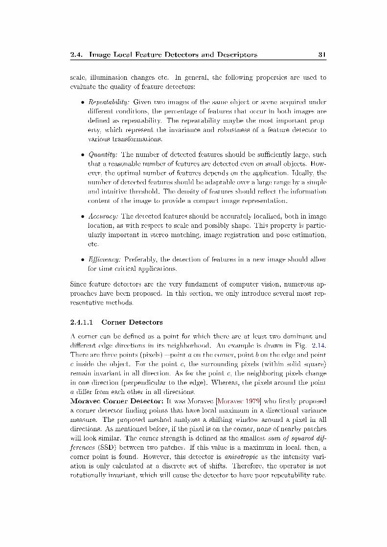
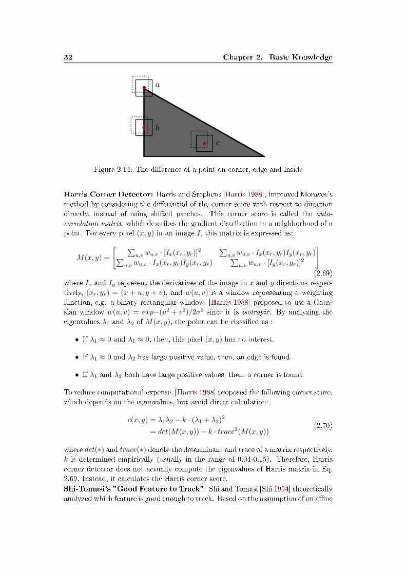
2.4.1.1 Corner Detectors
A corner can be de�ned as a point for which there are at least two dominant and
di�erent edge directions in its neighborhood. An example is drawn in Fig. 2.14.
There are three points (pixels) � point a on the corner, point b on the edge and point
c inside the object. For the point c, the surrounding pixels (within solid square)
remain invariant in all direction. As for the point c, the neighboring pixels change
in one direction (perpendicular to the edge). Whereas, the pixels around the point
a di�er from each other in all directions.
Moravec Corner Detector: It was Moravec [Moravec 1979] who �rstly proposed
a corner detector �nding points that have local maximum in a directional variance
measure. The proposed method analyzes a shifting window around a pixel in all
directions. As mentioned before, if the pixel is on the corner, none of nearby patches
will look similar. The corner strength is de�ned as the smallest sum of squared dif-
ferences (SSD) between two patches. If this value is a maximum in local, then, a
corner point is found. However, this detector is anisotropic as the intensity vari-
ation is only calculated at a discrete set of shifts. Therefore, the operator is not
rotationally invariant, which will cause the detector to have poor repeatability rate.
32 Chapter 2. Basic Knowledge
Figure 2.14: The di�erence of a point on corner, edge and inside
Harris Corner Detector: Harris and Stephens [Harris 1988], improved Moravec's
method by considering the di�erential of the corner score with respect to direction
directly, instead of using shifted patches. This corner score is called the auto-
correlation matrix, which describes the gradient distribution in a neighborhood of a
point. For every pixel (x, y) in an image I, this matrix is expressed as:
M(x, y) =
[
∑
u,v wu.v · [Ix(xr, yr)]2∑
u,v wu,v · Ix(xr, yr)Iy(xr, yr)∑
u,v wu,v · Ix(xr, yr)Iy(xr, yr)∑
u,v wu.v · [Iy(xr, yr)]2
]
(2.69)
where Ix and Iy represent the derivatives of the image in x and y directions respec-
tively, (xr, yr) = (x + u, y + v), and w(u, v) is a window representing a weighting
function, e.g. a binary rectangular window. [Harris 1988] proposed to use a Gaus-
sian window w(u, v) = exp−(u2 + v2)/2σ2 since it is isotropic. By analyzing the
eigenvalues λ1 and λ2 of M(x, y), the point can be classi�ed as :
• If λ1 ≈ 0 and λ1 ≈ 0, then, this pixel (x, y) has no interest.
• If λ1 ≈ 0 and λ2 has large positive value, then, an edge is found.
• If λ1 and λ2 both have large positive values, then, a corner is found.
To reduce computational expense, [Harris 1988] proposed the following corner score,
which depends on the eigenvalues, but avoid direct calculation:
c(x, y) = λ1λ2 − k · (λ1 + λ2)2
= det(M(x, y))− k · trace2(M(x, y))(2.70)
where det(∗) and trace(∗) denote the determinant and trace of a matrix respectively.
k is determined empirically (usually in the range of 0.04-0.15). Therefore, Harris
corner detector does not actually compute the eigenvalues of Harris matrix in Eq.
2.69. Instead, it calculates the Harris corner score.
Shi-Tomasi's "Good Feature to Track": Shi and Tomasi [Shi 1994] theoretically
analyzed which feature is good enough to track. Based on the assumption of an a�ne
2.4. Image Local Feature Detectors and Descriptors 33
image transformation, they found that it is more convenient and accurate to use the
smallest eigenvalue of the autocorrelation matrix as the corner score.
c(x, y) = min(λ1, λ2) > θ ·maxx,y
c(x, y) (2.71)
where θ is a prede�ned percentage factor to control the minimum score. Compared
to the Harris score (Eq. 2.70), this requires an additional square root computation
on each pixel.
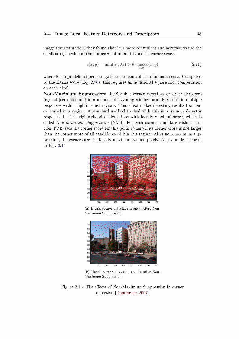
Non-Maximum Suppression: Performing corner detectors or other detectors
(e.g. object detectors) in a manner of scanning window usually results in multiple
responses within high interest regions. This e�ect makes detecting results too con-
centrated in a region. A standard method to deal with this is to remove detector
responses in the neighborhood of detections with locally maximal score, which is
called Non-Maximum Suppression (NMS). For each corner candidate within a re-
gion, NMS sets the corner score for this point to zero if its corner score is not larger
than the corner score of all candidates within this region. After non-maximum sup-
pression, the corners are the locally maximum valued pixels. An example is shown
in Fig. 2.15
(a) Harris corner detecting results before Non-
Maximum Suppression
(b) Harris corner detecting results after Non-
Maximum Suppression
Figure 2.15: The e�ects of Non-Maximum Suppression in corner
detection [Dominguez 2007]
34 Chapter 2. Basic Knowledge
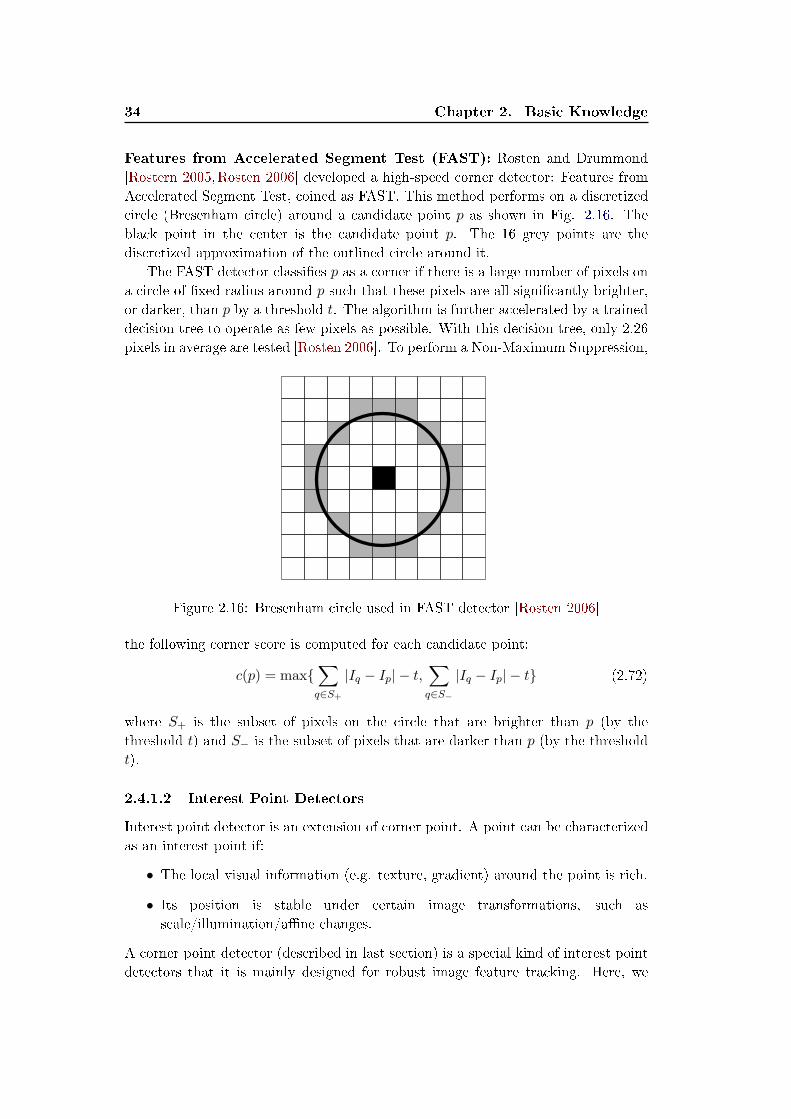
Features from Accelerated Segment Test (FAST): Rosten and Drummond
[Rostern 2005,Rosten 2006] developed a high-speed corner detector: Features from
Accelerated Segment Test, coined as FAST. This method performs on a discretized
circle (Bresenham circle) around a candidate point p as shown in Fig. 2.16. The
black point in the center is the candidate point p. The 16 grey points are the
discretized approximation of the outlined circle around it.
The FAST detector classi�es p as a corner if there is a large number of pixels on
a circle of �xed radius around p such that these pixels are all signi�cantly brighter,
or darker, than p by a threshold t. The algorithm is further accelerated by a trained
decision tree to operate as few pixels as possible. With this decision tree, only 2.26
pixels in average are tested [Rosten 2006]. To perform a Non-Maximum Suppression,
Figure 2.16: Bresenham circle used in FAST detector [Rosten 2006]
the following corner score is computed for each candidate point:
c(p) = max{∑
q∈S+
|Iq − Ip| − t,∑
q∈S−
|Iq − Ip| − t} (2.72)
where S+ is the subset of pixels on the circle that are brighter than p (by the
threshold t) and S− is the subset of pixels that are darker than p (by the threshold
t).
2.4.1.2 Interest Point Detectors
Interest point detector is an extension of corner point. A point can be characterized
as an interest point if:
• The local visual information (e.g. texture, gradient) around the point is rich.
• Its position is stable under certain image transformations, such as
scale/illumination/a�ne changes.
A corner point detector (described in last section) is a special kind of interest point
detectors that it is mainly designed for robust image feature tracking. Here, we
2.4. Image Local Feature Detectors and Descriptors 35
discuss more general cases of detecting interest points (or regions) for more general
tasks. Please note that in the history of computer vision, the applications of ter-
minologies "blob detector" and "interest point detector" are overlapping. Output
of blob detectors are usually well-de�ned point positions, which may correspond to
local extremas in an operation applied in local regions.
(a) Original image (b) The result of LoG(5× 5)
Figure 2.17: The e�ects of Laplacian of Gaussians
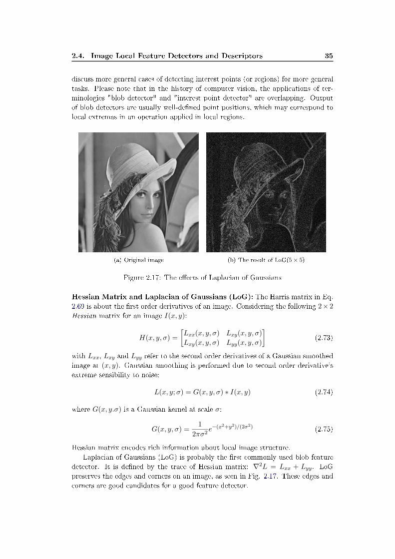
Hessian Matrix and Laplacian of Gaussians (LoG): The Harris matrix in Eq.
2.69 is about the �rst order derivatives of an image. Considering the following 2× 2
Hessian matrix for an image I(x, y):
H(x, y, σ) =
[
Lxx(x, y, σ) Lxy(x, y, σ)
Lxy(x, y, σ) Lyy(x, y, σ)
]
(2.73)
with Lxx, Lxy and Lyy refer to the second order derivatives of a Gaussian smoothed
image at (x, y). Gaussian smoothing is performed due to second order derivative's
extreme sensibility to noise:
L(x, y;σ) = G(x, y, σ) ∗ I(x, y) (2.74)
where G(x, y.σ) is a Gaussian kernel at scale σ:
G(x, y, σ) =1
2πσ2e−(x2+y2)/(2σ2) (2.75)
Hessian matrix encodes rich information about local image structure.
Laplacian of Gaussians (LoG) is probably the �rst commonly used blob feature
detector. It is de�ned by the trace of Hessian matrix: ∇2L = Lxx + Lyy. LoG
preserves the edges and corners on an image, as seen in Fig. 2.17. These edges and
corners are good candidates for a good feature detector.
36 Chapter 2. Basic Knowledge
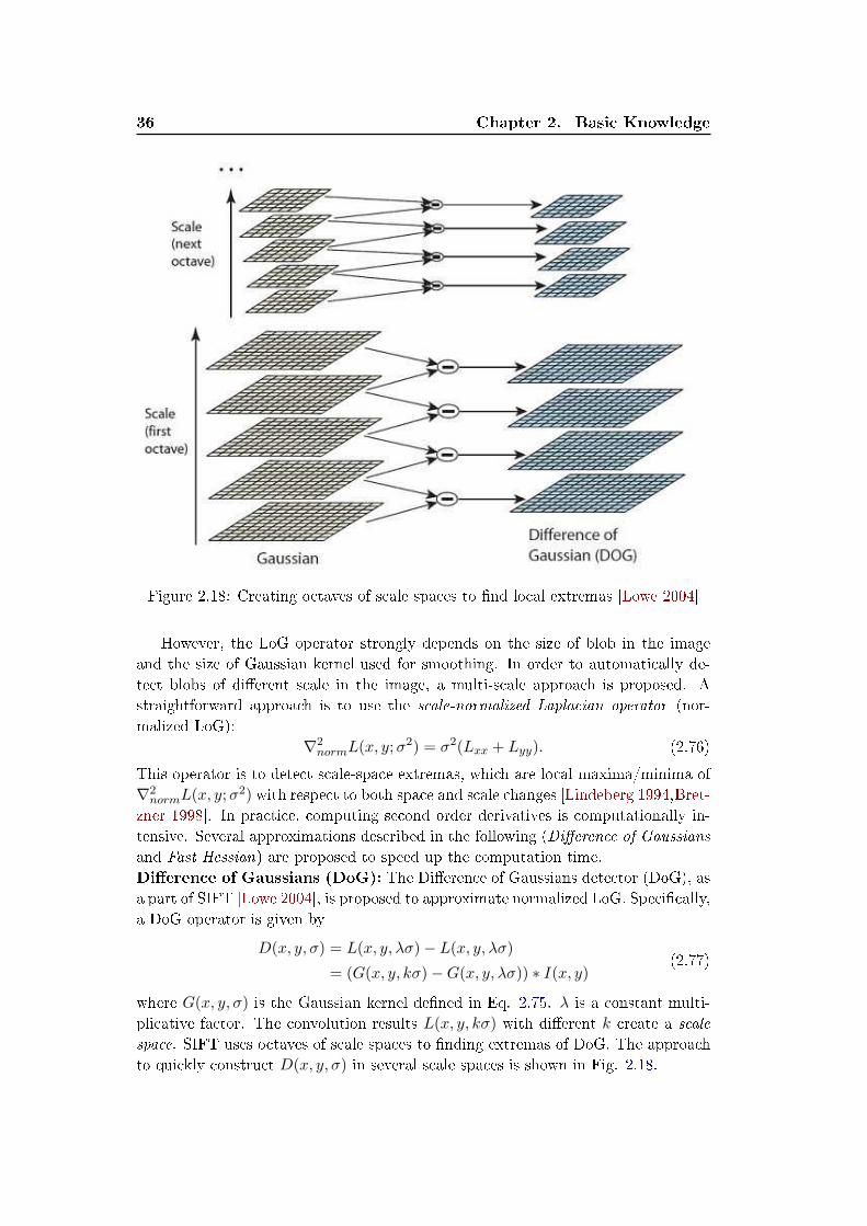
Figure 2.18: Creating octaves of scale spaces to �nd local extremas [Lowe 2004]
However, the LoG operator strongly depends on the size of blob in the image
and the size of Gaussian kernel used for smoothing. In order to automatically de-
tect blobs of di�erent scale in the image, a multi-scale approach is proposed. A
straightforward approach is to use the scale-normalized Laplacian operator (nor-
malized LoG):
∇2normL(x, y;σ2) = σ2(Lxx + Lyy). (2.76)
This operator is to detect scale-space extremas, which are local maxima/minima of
∇2normL(x, y;σ2) with respect to both space and scale changes [Lindeberg 1994,Bret-
zner 1998]. In practice, computing second order derivatives is computationally in-
tensive. Several approximations described in the following (Di�erence of Gaussians
and Fast Hessian) are proposed to speed up the computation time.
Di�erence of Gaussians (DoG): The Di�erence of Gaussians detector (DoG), as
a part of SIFT [Lowe 2004], is proposed to approximate normalized LoG. Speci�cally,
a DoG operator is given by
D(x, y, σ) = L(x, y, λσ)− L(x, y, λσ)
= (G(x, y, kσ)−G(x, y, λσ)) ∗ I(x, y)(2.77)
where G(x, y, σ) is the Gaussian kernel de�ned in Eq. 2.75. λ is a constant multi-
plicative factor. The convolution results L(x, y, kσ) with di�erent k create a scale
space. SIFT uses octaves of scale spaces to �nding extremas of DoG. The approach
to quickly construct D(x, y, σ) in several scale spaces is shown in Fig. 2.18.
2.4. Image Local Feature Detectors and Descriptors 37
For each octave of scale space, the initial image is repeately convolved with
Gaussians to produce the set of scale space images shown on the left of Fig. 2.18.
Adjacent Gaussian images are subtracted to produce the di�erence-of-Gaussian im-
ages on the right of Fig. 2.18. After processing each octave, the Gaussian image
is down-sampled by a factor of 2, and the process repeated. Key points are then
extracted at local minima/maxima of the DoG images through scales.
The DoG approximation greatly reduces the computation cost � it can be com-
puted by a simple image subtraction. As an approximation of normalized LoG
operator, DoG is scale invariant.
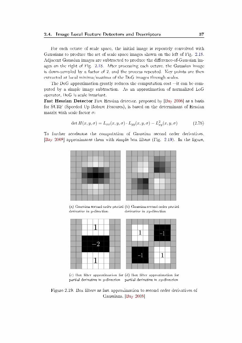
Fast Hessian Detector Fast Hessian detector, proposed by [Bay 2008] as a basis
for SURF (Speeded Up Robust Features), is based on the determinant of Hessian
matrix with scale factor σ:
detH(x, y, σ) = Lxx(x, y, σ) · Lyy(x, y, σ)− L2xy(x, y, σ) (2.78)
To further accelerate the computation of Gaussian second order derivatives,
[Bay 2008] approximates them with simple box �lters (Fig. 2.19). In the �gure,
(a) Gaussian second order partial
derivative in y-direction
(b) Gaussian second order partial
derivative in xy-direction
(c) Box �lter approximation for
partial derivative in y-direction
(d) Box �lter approximation for
partial derivative in xy-direction
Figure 2.19: Box �lters as fast approximation to second order derivatives of
Gaussians. [Bay 2008]
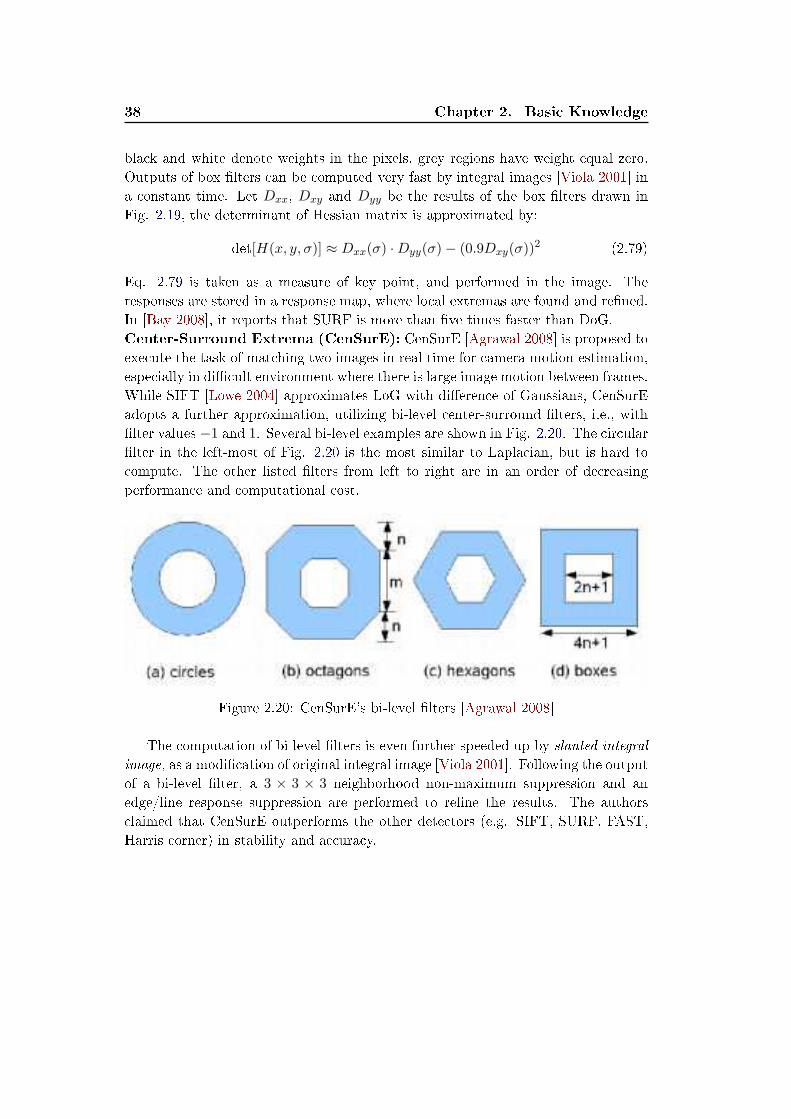
38 Chapter 2. Basic Knowledge
black and white denote weights in the pixels, grey regions have weight equal zero.
Outputs of box �lters can be computed very fast by integral images [Viola 2001] in
a constant time. Let Dxx, Dxy and Dyy be the results of the box �lters drawn in
Fig. 2.19, the determinant of Hessian matrix is approximated by:
det[H(x, y, σ)] ≈ Dxx(σ) ·Dyy(σ)− (0.9Dxy(σ))2 (2.79)
Eq. 2.79 is taken as a measure of key point, and performed in the image. The
responses are stored in a response map, where local extremas are found and re�ned.
In [Bay 2008], it reports that SURF is more than �ve times faster than DoG.
Center-Surround Extrema (CenSurE): CenSurE [Agrawal 2008] is proposed to
execute the task of matching two images in real time for camera motion estimation,
especially in di�cult environment where there is large image motion between frames.
While SIFT [Lowe 2004] approximates LoG with di�erence of Gaussians, CenSurE
adopts a further approximation, utilizing bi-level center-surround �lters, i.e., with
�lter values −1 and 1. Several bi-level examples are shown in Fig. 2.20. The circular
�lter in the left-most of Fig. 2.20 is the most similar to Laplacian, but is hard to
compute. The other listed �lters from left to right are in an order of decreasing
performance and computational cost.
Figure 2.20: CenSurE's bi-level �lters [Agrawal 2008]
The computation of bi-level �lters is even further speeded up by slanted integral
image, as a modi�cation of original integral image [Viola 2001]. Following the output
of a bi-level �lter, a 3 × 3 × 3 neighborhood non-maximum suppression and an
edge/line response suppression are performed to re�ne the results. The authors
claimed that CenSurE outperforms the other detectors (e.g. SIFT, SURF, FAST,
Harris corner) in stability and accuracy.
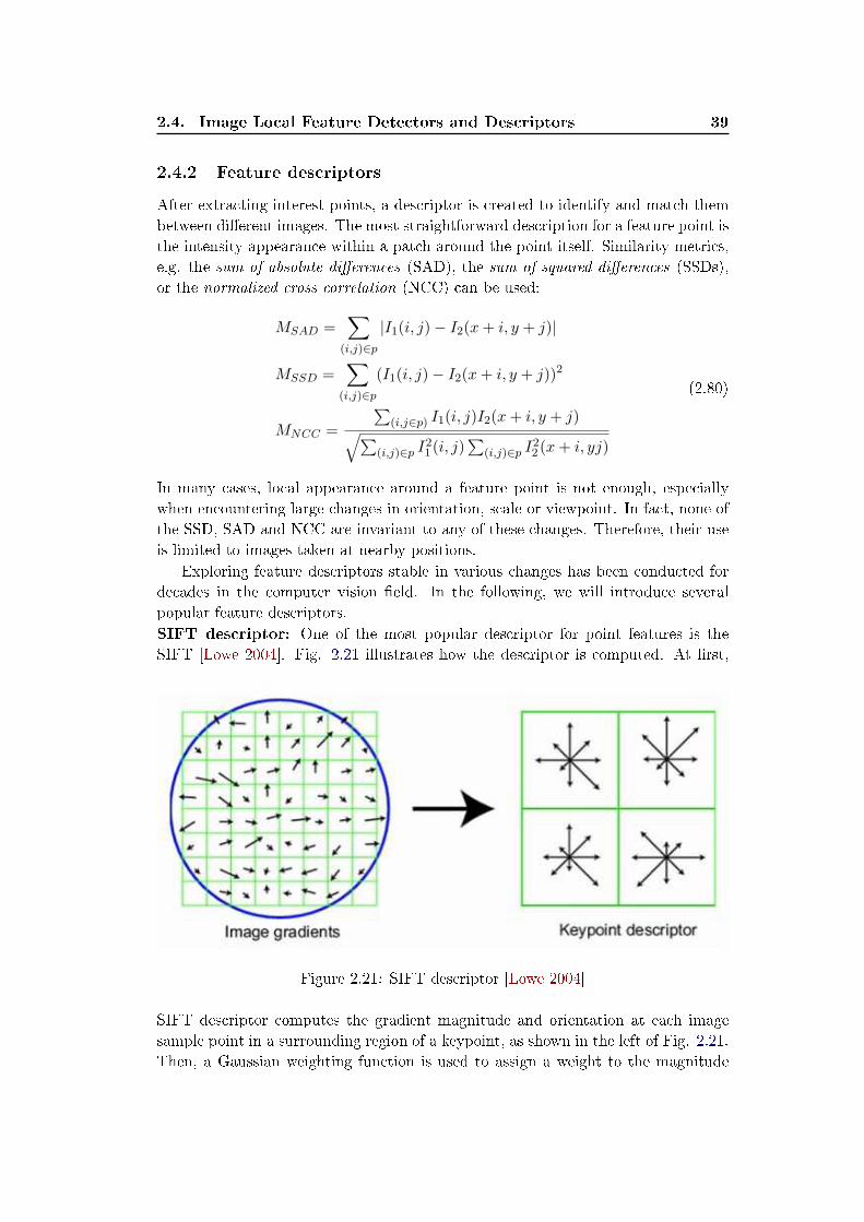
2.4. Image Local Feature Detectors and Descriptors 39
2.4.2 Feature descriptors
After extracting interest points, a descriptor is created to identify and match them
between di�erent images. The most straightforward description for a feature point is
the intensity appearance within a patch around the point itself. Similarity metrics,
e.g. the sum of absolute di�erences (SAD), the sum of squared di�erences (SSDs),
or the normalized cross correlation (NCC) can be used:
MSAD =∑
(i,j)∈p
|I1(i, j)− I2(x+ i, y + j)|
MSSD =∑
(i,j)∈p
(I1(i, j)− I2(x+ i, y + j))2
MNCC =
∑
(i,j∈p) I1(i, j)I2(x+ i, y + j)√
∑
(i,j)∈p I21 (i, j)
∑
(i,j)∈p I22 (x+ i, yj)
(2.80)
In many cases, local appearance around a feature point is not enough, especially
when encountering large changes in orientation, scale or viewpoint. In fact, none of
the SSD, SAD and NCC are invariant to any of these changes. Therefore, their use
is limited to images taken at nearby positions.
Exploring feature descriptors stable in various changes has been conducted for
decades in the computer vision �eld. In the following, we will introduce several
popular feature descriptors.
SIFT descriptor: One of the most popular descriptor for point features is the
SIFT [Lowe 2004]. Fig. 2.21 illustrates how the descriptor is computed. At �rst,
Figure 2.21: SIFT descriptor [Lowe 2004]
SIFT descriptor computes the gradient magnitude and orientation at each image
sample point in a surrounding region of a keypoint, as shown in the left of Fig. 2.21.
Then, a Gaussian weighting function is used to assign a weight to the magnitude
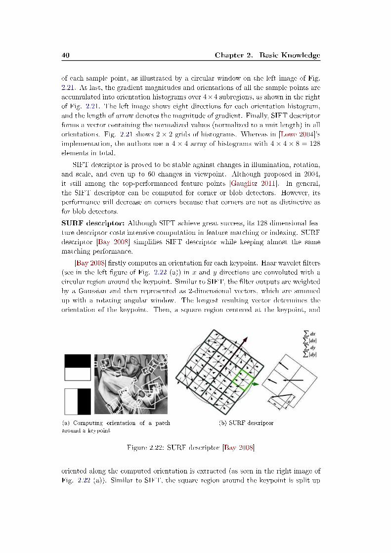
40 Chapter 2. Basic Knowledge
of each sample point, as illustrated by a circular window on the left image of Fig.
2.21. At last, the gradient magnitudes and orientations of all the sample points are
accumulated into orientation histograms over 4×4 subregions, as shown in the right
of Fig. 2.21. The left image shows eight directions for each orientation histogram,
and the length of arrow denotes the magnitude of gradient. Finally, SIFT descriptor
forms a vector containing the normalized values (normalized to a unit length) in all
orientations. Fig. 2.21 shows 2 × 2 grids of histograms. Whereas in [Lowe 2004]'s
implementation, the authors use a 4 × 4 array of histograms with 4 × 4 × 8 = 128
elements in total.
SIFT descriptor is proved to be stable against changes in illumination, rotation,
and scale, and even up to 60 changes in viewpoint. Although proposed in 2004,
it still among the top-performanced feature points [Gauglitz 2011]. In general,
the SIFT descriptor can be computed for corner or blob detectors. However, its
performance will decrease on corners because that corners are not as distinctive as
for blob detectors.
SURF descriptor: Although SIFT achieve great success, its 128-dimensional fea-
ture descriptor costs intensive computation in feature matching or indexing. SURF
descriptor [Bay 2008] simpli�es SIFT descriptor while keeping almost the same
matching performance.
[Bay 2008] �rstly computes an orientation for each keypoint. Haar wavelet �lters
(see in the left �gure of Fig. 2.22 (a)) in x and y directions are convoluted with a
circular region around the keypoint. Similar to SIFT, the �lter outputs are weighted
by a Gaussian and then represented as 2-dimensional vectors, which are summed
up with a rotating angular window. The longest resulting vector determines the
orientation of the keypoint. Then, a square region centered at the keypoint, and
(a) Computing orientation of a patch
around a keypoint
(b) SURF descriptor
Figure 2.22: SURF descriptor [Bay 2008]
oriented along the computed orientation is extracted (as seen in the right image of
Fig. 2.22 (a)). Similar to SIFT, the square region around the keypoint is split up
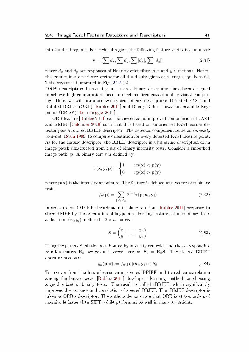
2.4. Image Local Feature Detectors and Descriptors 41
into 4× 4 subregions. For each subregion, the following feature vector is computed:
v = [∑
dx,∑
dy,∑
|dx|,∑
|dy|] (2.81)
where dx and dy are responses of Haar wavelet �lter in x and y directions. Hence,
this results in a descriptor vector for all 4 × 4 subregions of a length equals to 64.
This process is illustrated in Fig. 2.22 (b).
ORB descriptor: In recent years, several binary descriptors have been designed
to achieve high computation speed to meet requirements of mobile visual comput-
ing. Here, we will introduce two typical binary descriptors: Oriented FAST and
Rotated BRIEF (ORB) [Rublee 2011] and Binary Robust Invariant Scalable Key-
points (BRISK) [Leutenegger 2011].
ORB feature [Rublee 2011] can be viewed as an improved combination of FAST
and BRIEF [Calonder 2010] such that it is based on an oriented FAST corner de-
tector plus a rotated BRIEF descriptor. The detector component relies on intensity
centroid [Rosin 1999] to compute orientation for every detected FAST feature point.
As for the feature descriptor, the BRIEF descriptor is a bit string description of an
image patch constructed from a set of binary intensity tests. Consider a smoothed
image path, p. A binary test τ is de�ned by:
τ(x,y;p) =
{
1 : p(x) < p(y)
0 : p(x) > p(y)
where p(x) is the intensity at point x. The feature is de�ned as a vector of n binary
tests:
fn(p) =∑
1≤i≤n
2i−1τ(p;xi,yi) (2.82)
In order to let BRIEF be invariant to in-plane rotation, [Rublee 2011] proposed to
steer BRIEF by the orientation of keypoints. For any feature set of n binary tests
at location (xi, yi), de�ne the 2× n matrix:
S =
(
x1 · · · xny1 · · · yn
)
(2.83)
Using the patch orientation θ estimated by intensity centroid, and the corresponding
rotation matrix Rθ, we get a "steered" version Sθ = RθS. The steered BRIEF
operator becomes:
gn(p, θ) := fn(p)|(xi,yi) ∈ Sθ (2.84)
To recover from the loss of variance in steered BRIEF and to reduce correlation
among the binary tests, [Rublee 2011] develops a learning method for choosing
a good subset of binary tests. The result is called rBRIEF, which signi�cantly
improves the variance and correlation of steered BRIEF. The rBRIEF descriptor is
taken as ORB's descriptor. The authors demonstrate that ORB is at two orders of
magnitude faster than SIFT, while performing as well in many situations.
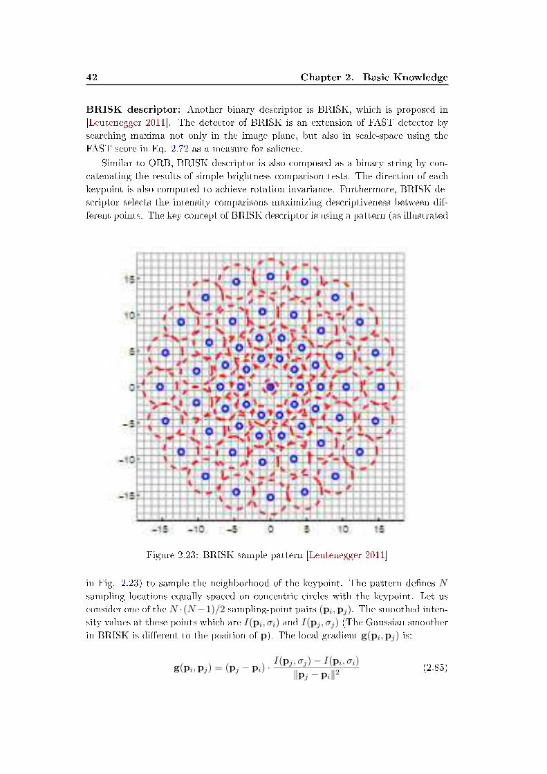
42 Chapter 2. Basic Knowledge
BRISK descriptor: Another binary descriptor is BRISK, which is proposed in
[Leutenegger 2011]. The detector of BRISK is an extension of FAST detector by
searching maxima not only in the image plane, but also in scale-space using the
FAST score in Eq. 2.72 as a measure for salience.
Similar to ORB, BRISK descriptor is also composed as a binary string by con-
catenating the results of simple brightness comparison tests. The direction of each
keypoint is also computed to achieve rotation invariance. Furthermore, BRISK de-
scriptor selects the intensity comparisons maximizing descriptiveness between dif-
ferent points. The key concept of BRISK descriptor is using a pattern (as illustrated
Figure 2.23: BRISK sample pattern [Leutenegger 2011]
in Fig. 2.23) to sample the neighborhood of the keypoint. The pattern de�nes N
sampling locations equally spaced on concentric circles with the keypoint. Let us
consider one of the N ·(N−1)/2 sampling-point pairs (pi,pj). The smoothed inten-
sity values at these points which are I(pi, σi) and I(pj , σj) (The Gaussian smoother
in BRISK is di�erent to the position of p). The local gradient g(pi,pj) is:
g(pi,pj) = (pj − pi) ·I(pj , σj)− I(pi, σi)
∥pj − pi∥2(2.85)
2.4. Image Local Feature Detectors and Descriptors 43
Considering the set A of all sampling-point pairs, the authors de�ne a subset S of
short-distance pairing and another subset L of long-distance pairings:
S = {(pi,pj) ∈ A| ||pj − pi|| < σmax} ⊆ AL = {(pi,pj) ∈ A| ||pj − pi|| > σmin} ⊆ A
(2.86)
The pattern direction is estimated through the point pairs in L:
g =
(
gxgy
)
=1
L·
∑
pi,pj∈L
g(pi,pj) (2.87)
where L is the number of point pairs. In order to make a rotation and scale normal-
ized descriptor, BRISK rotates the sampling pattern by α = arctan 2(gx.gy) around
a keypoint. The bit-string descriptor is created by comparing all the short distance
intensity comparisons:
b =
{
1 I(pαj , σj) > I(pα
j , σi) (pαi ,p
αj ) ∈ S
0 otherwise
The experiments in [Leutenegger 2011] reveal BRISK's high quality performance as
in state-of-art algorithms, with a lower computational cost.
2.4.3 Associating feature points through images
As described in the beginning of Sec. 2.4, one of the most important need when
using image feature points is to stable localizing the same point through di�erent
image. Many computer vision applications, e.g. stereo matching, pose estimation,
augmented reality and object recognition, are relied on precise feature point associ-
ating. In this section, we introduce two approaches to associate feature points: the
�rst is feature tracking, the second is feature matching.
2.4.3.1 Kanade-Lucas-Tomasi Tracking (KLT tracker)
KLT tracker is a classic image feature point tracking algorithm in computer vision
area. It is based on the early work of [Lucas 1981], then is developed fully by
[Tomasi 1991], and is explained in details in [Shi 1994]. Later, [Bouguet 2000] gives
a pyramidal implementation to cope with large displacement.
Let two images I(x) = I(x, y), J(x) = J(x, y) refer to the �rst image and second
one, respectively. For an image point u = [ux, uy] on the �rst image I, KLT tracker
is to �nd its corresponding location v = u+ d = [ux + dx, uy + dy]T on the second
image J . Let W(x;p) be the warp from image I to J , where p is a vector of
parameters. The best alignment minimizes image dissimilarity:
∑
[I(W(x;p))− J(x)]2 (2.88)
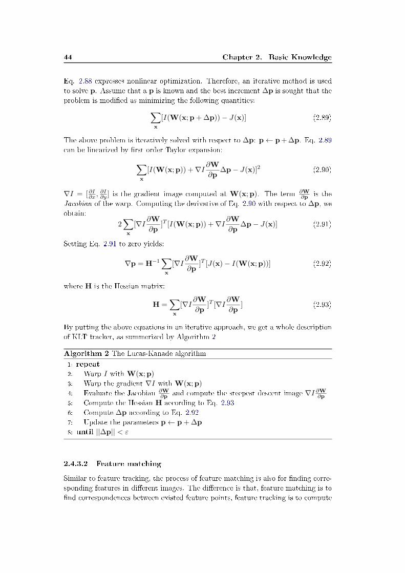
44 Chapter 2. Basic Knowledge
Eq. 2.88 expresses nonlinear optimization. Therefore, an iterative method is used
to solve p. Assume that a p is known and the best increment ∆p is sought that the
problem is modi�ed as minimizing the following quantities:
∑
x
[I(W(x;p+∆p))− J(x)] (2.89)
The above problem is iteratively solved with respect to ∆p: p← p+∆p. Eq. 2.89
can be linearized by �rst order Taylor expansion:
∑
x
[I(W(x;p)) +∇I ∂W∂p
∆p− J(x)]2 (2.90)
∇I = [ ∂I∂x ,∂I∂y ] is the gradient image computed at W(x;p). The term ∂W
∂p is the
Jacobian of the warp. Computing the derivative of Eq. 2.90 with respect to ∆p, we
obtain:
2∑
x
[∇I ∂W∂p
]T [I(W(x;p)) +∇I ∂W∂p
∆p− J(x)] (2.91)
Setting Eq. 2.91 to zero yields:
∇p = H−1∑
x
[∇I ∂W∂p
]T [J(x)− I(W(x;p))] (2.92)
where H is the Hessian matrix:
H =∑
x
[∇I ∂W∂p
]T [∇I ∂W∂p
] (2.93)
By putting the above equations in an iterative approach, we get a whole description
of KLT tracker, as summerized by Algorithm 2
Algorithm 2 The Lucas-Kanade algorithm
1: repeat2: Warp I with W(x;p)
3: Warp the gradient ∇I with W(x;p)
4: Evaluate the Jacobian ∂W∂p and compute the steepest descent image ∇I ∂W
∂p
5: Compute the Hessian H according to Eq. 2.93
6: Compute ∆p according to Eq. 2.92
7: Update the parameters p← p+∆p
8: until ||∆p|| < ε
2.4.3.2 Feature matching
Similar to feature tracking, the process of feature matching is also for �nding corre-
sponding features in di�erent images. The di�erence is that, feature matching is to
�nd correspondences between existed feature points, feature tracking is to compute
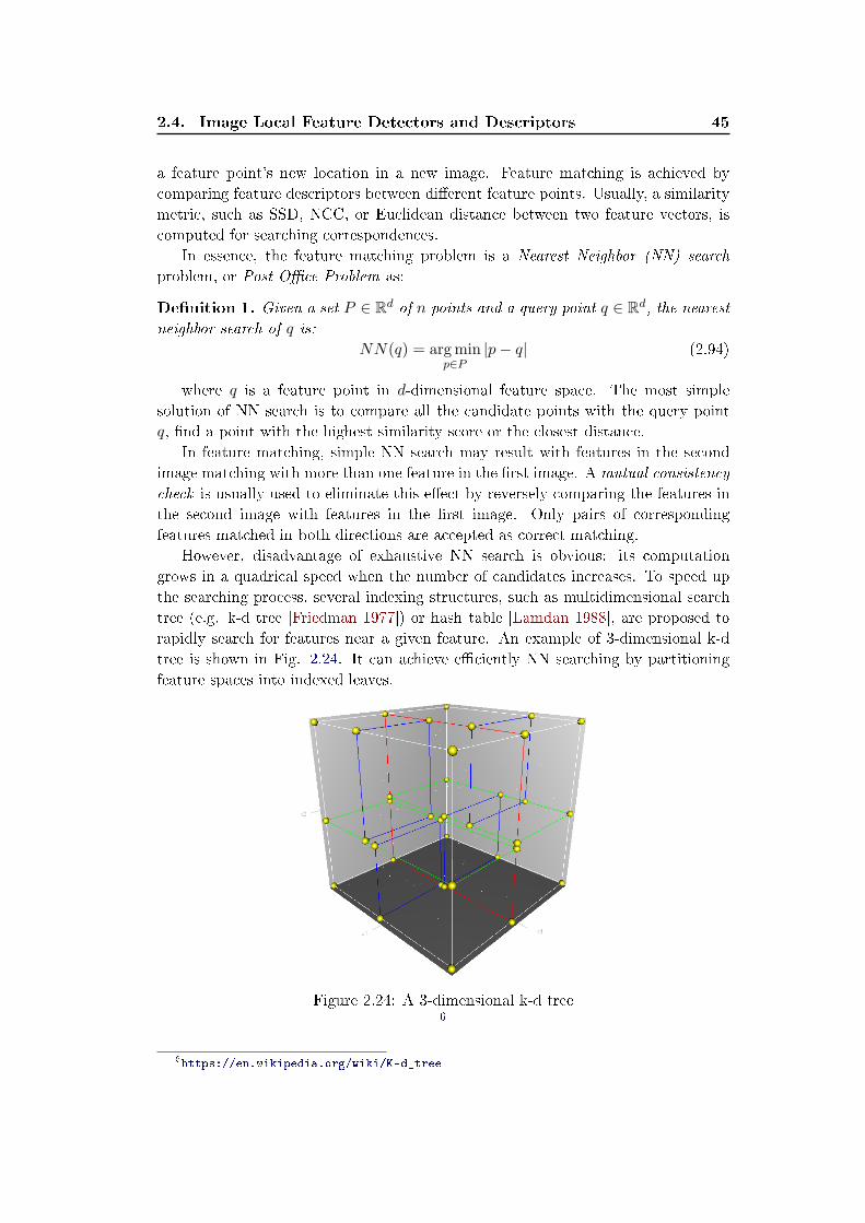
2.4. Image Local Feature Detectors and Descriptors 45
a feature point's new location in a new image. Feature matching is achieved by
comparing feature descriptors between di�erent feature points. Usually, a similarity
metric, such as SSD, NCC, or Euclidean distance between two feature vectors, is
computed for searching correspondences.
In essence, the feature matching problem is a Nearest Neighbor (NN) search
problem, or Post O�ce Problem as:
De�nition 1. Given a set P ∈ Rd of n points and a query point q ∈ R
d, the nearest
neighbor search of q is:
NN(q) = argminp∈P
|p− q| (2.94)
where q is a feature point in d-dimensional feature space. The most simple
solution of NN search is to compare all the candidate points with the query point
q, �nd a point with the highest similarity score or the closest distance.
In feature matching, simple NN search may result with features in the second
image matching with more than one feature in the �rst image. A mutual consistency
check is usually used to eliminate this e�ect by reversely comparing the features in
the second image with features in the �rst image. Only pairs of corresponding
features matched in both directions are accepted as correct matching.
However, disadvantage of exhaustive NN search is obvious: its computation
grows in a quadrical speed when the number of candidates increases. To speed up
the searching process, several indexing structures, such as multidimensional search
tree (e.g. k-d tree [Friedman 1977]) or hash table [Lamdan 1988], are proposed to
rapidly search for features near a given feature. An example of 3-dimensional k-d
tree is shown in Fig. 2.24. It can achieve e�ciently NN searching by partitioning
feature spaces into indexed leaves.
Figure 2.24: A 3-dimensional k-d tree6
6https://en.wikipedia.org/wiki/K-d_tree
46 Chapter 2. Basic Knowledge
An another feature matching strategy is to search for potential correspondences
in an expecting region in the second image. The size of regions can be prede�ned
or predicted by the motion model of feature points. More works can be refered
in [Chili 2008,Handa 2010].
2.5 Conclusion
In this chapter, we �rstly describe the stereo vision measurement model. Since
our stereo vision system consists of two quasi-parallel monocular camera, the stereo
vision measurement model is based on monocular camera pinhole model. The distor-
tion model of the lens is also considered. The stereo vision model is very important
and forms the basis of many further application in the following chapters.
In the second, we review second linear/non-linear least squares methods. These
methods are commonly used to solve estimation problems. For linear least square
methods, ordinary and total least squares methods are introduced. Ordinary least
squares are widely used in many computer vision problems, while the total least
squares is an improved version of least squares when considering all the errors.
For non-linear least squares, Gaussian-Newton method and Levenberg-Marquardt
algorithm are described. We will use these two methods to estimate parameters in
the following chapters.
At last, we present an overview of feature detectors/descriptors. In litera-
ture, a lot of feature detectors/descriptors are proposed because of wide applica-
tions. The number of proposed feature detectors/descriptors is so big that many
researchers often feel confused. We try to summarize the development of feature de-
tectors/descriptors by di�erent categories. In the following chapter, we will analyze
their performances in visual odometry.
Chapter 3
Stereo Vision based Ego-motion
Estimation
Contents
3.1 Introduction . . . . . . . . . . . . . . . . . . . . . . . . . . . . 48
3.2 Circular Feature Points Detection and Association . . . . . 50
3.2.1 Circular Feature Point Association by KLT Tracker . . . . . 51
3.2.2 Circular Feature Point Association by Matching . . . . . . . 51
3.3 Ego-motion Computation . . . . . . . . . . . . . . . . . . . . . 54
3.3.1 3D-2D Constraint based Ego-motion Estimation . . . . . . . 54
3.4 Experiments of Stereo Visual Odometry . . . . . . . . . . . 57
3.4.1 Comparing Di�erent Feature Association Approaches . . . . 57
3.4.2 Stereo Visual Odometry in Urban Environment . . . . . . . . 62
3.5 Conclusion and Future Works . . . . . . . . . . . . . . . . . . 70
In this chapter, we provide a stereo vision based method to estimate the ego-
motion of a moving intelligent vehicle in urban environments. Estimation of self-
motion is important for an intelligent vehicle since:
• It provides a complementary localizing approach for GPS. In urban environ-
ments, GPS signals could disappear or be disturbed due to buildings, tunnels,
etc. Without any prior knowledge of the environment nor a prede�ned mo-
tion model of the vehicle, vision based ego-motion estimation can estimate
the path of a camera-equipped vehicle by calculating the ego-motion between
consecutive images in a video �ow. Hence, vision based ego-motion estimation
could be used for vehicle localization when GPS signals are not available.
• It is the fundament of further analyzing of a dynamic environment. When the
intelligent vehicle is driving in a dynamic environment, understanding self-
motion is the �rst step before performing independent moving object detection,
tracking and recognition.
In this chapter, we present a stereo vision based method to estimate the ego-motion
of a moving intelligent vehicle. The contributions are comparing tracking based ap-
proaches with matching based approaches, as well as performances di�erent feature
detectors. The objective is to select the best feature point detector and the best
circular point association for urban environment perception.
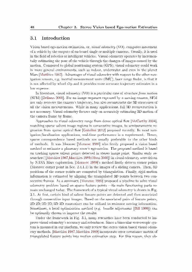
48 Chapter 3. Stereo Vision based Ego-motion Estimation
3.1 Introduction
Vision based ego-motion estimation, or, visual odometry (VO), computes movement
of a vehicle by the outputs of on-board single or multiple cameras. Usually, it is used
in the �eld of robotics or intelligent vehicles. Visual odometry operates by incremen-
tally estimating the pose of the vehicle through the changes of images caused by the
motion. Compared to global positioning system (GPS), visual odometry could work
in more general environments, such as indoor, underwater and even in the planet
Mars [Matthies 1987]. Advantages of visual odometry with respect to the other nav-
igation sensors, e.g. inertial measurement units (IMU), laser range �nder, is that it
is not a�ected by wheel slip and it provides more accurate trajectory estimates in a
low expense.
In literature, visual odometry (VO) is a particular case of structure from motion
(SFM) [Dellaert 2000]. For an image sequence captured by a moving camera, SFM
not only recovers the camera's trajectory, but also reconstructs the 3D structures of
all the vision measurements. While in many applications, full 3D reconstruction is
not necessary. Visual odometry focuses only on accurately estimating 3D motion of
the camera frame by frame.
Approaches to visual odometry range from dense optical �ow [McCarthy 2004],
matching sparse salient image regions in consecutive images, to semiparametric re-
gression from sparse optical �ow [Guizilini 2012] proposed recently. In most nav-
igation/localization applications, real-time performance is a requirement. Hence,
sparse correspondence based methods are usually preferable to the other kinds
of methods. It was Moravec [Moravec 1980] who �rstly proposed a vision-based
method to estimate a planetary rover's ego-motion. The proposed method is based
on tracking sparse salient points detected in stereo image pairs. Similar early re-
searches ( [Matthies 1987,Matthies 1989,Olson 2000]) in visual odometry were driven
by NASA Mars exploration. [Moravec 1980]'s method �rstly detects corner points
(Moravec corner point in Sec. 2.4.1.1) in the images of a sliding camera. Then, 3D
positions of the corner points are computed by triangulation. Finally, rigid motion
information is estimated by aligning the triangulated 3D points between two con-
secutive frames. As a summary, [Moravec 1980] proposed a pipeline to solve visual
odometry problem based on sparse feature points � its main functioning parts re-
main unchanged today. The framework of a typical visual odometry is drawn in Fig.
3.1. At �rst, certain kind of salient feature points are detected and then associated
through consecutive input images. Based on the associated pairs of feature points,
2D-2D/3D-2D/3D-3D constraints can be utilized to estimate moving information.
Sometimes, a local optimization method (e.g. bundle adjustment [Bill 1999]) can
be optionally chosen to improve the results.
Under the framework in Fig. 3.1, many researches have been conducted to im-
prove visual odometry's accuracy and robustness. Since a binocular stereoscopic sys-
tem is mounted in our platform, we only review the stereo vision based visual odom-
etry methods. [Matthies 1987,Matthies 1989] incorporate error covariance matrix of
triangulated feature points into motion estimation step. For this reason, they ob-
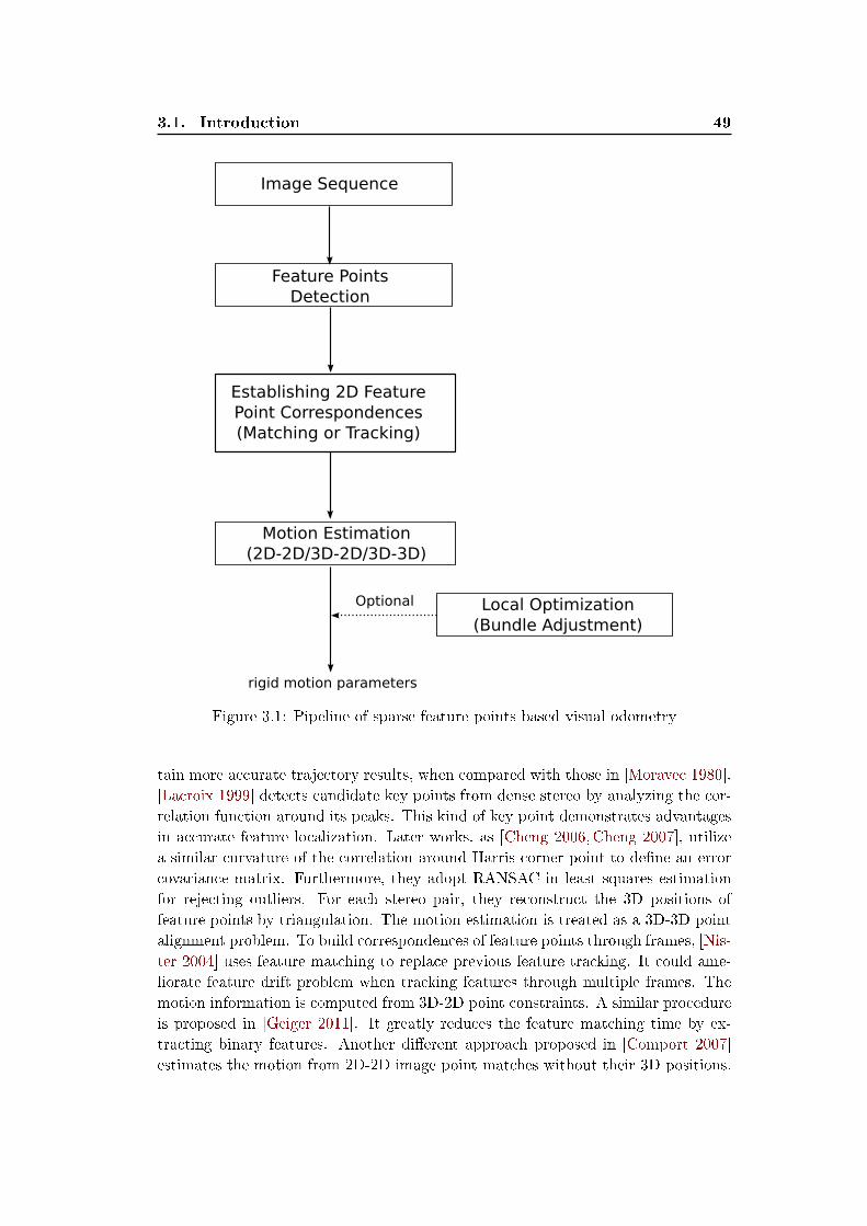
3.1. Introduction 49
Image Sequence
Feature Points
Detection
Establishing 2D Feature
Point Correspondences
(Matching or Tracking)
Motion Estimation
(2D-2D/3D-2D/3D-3D)
Local Optimization
(Bundle Adjustment)
Optional
rigid motion parameters
Figure 3.1: Pipeline of sparse feature points based visual odometry
tain more accurate trajectory results, when compared with those in [Moravec 1980].
[Lacroix 1999] detects candidate key points from dense stereo by analyzing the cor-
relation function around its peaks. This kind of key point demonstrates advantages
in accurate feature localization. Later works, as [Cheng 2006,Cheng 2007], utilize
a similar curvature of the correlation around Harris corner point to de�ne an error
covariance matrix. Furthermore, they adopt RANSAC in least squares estimation
for rejecting outliers. For each stereo pair, they reconstruct the 3D positions of
feature points by triangulation. The motion estimation is treated as a 3D-3D point
alignment problem. To build correspondences of feature points through frames, [Nis-
ter 2004] uses feature matching to replace previous feature tracking. It could ame-
liorate feature drift problem when tracking features through multiple frames. The
motion information is computed from 3D-2D point constraints. A similar procedure
is proposed in [Geiger 2011]. It greatly reduces the feature matching time by ex-
tracting binary features. Another di�erent approach proposed in [Comport 2007]
estimates the motion from 2D-2D image point matches without their 3D positions.
50 Chapter 3. Stereo Vision based Ego-motion Estimation
This solution derives from a "quadrifocal tensor". The authors claim that more ac-
curate motion estimation could be reached by the 2D-2D based motion estimation.
In the following, we will follow the framework of classic stereo visual odometry
to estimate vehicle's ego-motion. The contribution of our works is the comparison of
various feature detectors and the di�erent approaches of circular feature association.
3.2 Circular Feature Points Detection and Association
The objectives of this section are �nding local invariant salient points in successive
stereo image pairs and establishing their mutual correspondences. As illustrated
in Fig. 3.1, these steps provide necessary information for the following motion
estimation. In our practice, we detect and associate the feature points in a circu-
lar manner as in [Geiger 2011]. For an acquired stereo image pair at time t − 1
and t, circular point-to-point correspondences are established in all the four im-
ages: current left/right images and previous left/right images. This is depicted
in Fig. 3.2. In this step, a feature point (utl , vtl ) detected in the current left im-
age at time t is associated with corresponding locations in the other images as:
(utr, vtr), (u
t−1l , vt−1
l ), (ut−1r , vt−1
r ). Therefore, the four positions of a same point in
four images form a circle: (utl , vtl )↔ (utr, v
tr)↔ (ut−1
l , vt−1l )↔ (ut−1
r , vt−1r )
t-1 t
Left
Image
Right
Image
Time: t+1
...
...
...
Figure 3.2: Circularly association of detected feature points in consecutive image
pairs
In Sec. 2.4, we have reviewed several commonly used image local detectors,
descriptors, as well as tracking and matching approaches. To seek a circular point-
to-point correspondences between successive images, two distinct approaches are
possible:
• The �rst approach is to detect feature points in one image, then, track the
detected points in other images.
3.2. Circular Feature Points Detection and Association 51
• The second approach is to detect feature points in all the four images, then,
match these points by their feature descriptors.
3.2.1 Circular Feature Point Association by KLT Tracker
Kanade-Lucas-Tomasi (KLT) tracker (described in Sec. 2.4.3.1) is the most popular
point tracking method in the computer vision �eld. KLT tracker is able to accu-
rately track a point, especially a corner point, by directly using spatial intensity
information. In circular feature point association, feature points (e.g. Harris cor-
ners) are �rstly detected in the the current left image. Then, they are tracked in
two di�erent ways to formulate a circle. Let ptl be a feature point in the current left
image. The �rst way tracks ptl in the current right image to ptr, then in previous
right image to pt−1r and �nally in the previous left image to pt−1
l ; the second way
directly tracks ptl in the previous left image to p′t−1l from the current left image. If
the displacement between pt−1l and p′t−1
l is within a tolerance range, the circular
tracking is succeeded. Otherwise, the KLT tracker failed to track this point within a
circle. An example of KLT tracker based circular point association is demonstrated
in Fig. 3.3 (a). The yellow circle shows a successfully circularly tracked feature
point ptl,1 from the current left image to the other three images. The green circle
shows an unsuccessfully tracked circle due to unacceptable displacement.
3.2.2 Circular Feature Point Association by Matching
As for feature matching based circular feature point association, feature points and
their descriptors are computed separately in all the four images. Given a feature
point ptl in the current left image, we search its correspondences in the other three
images by comparing their descriptors. To avoid exhaustive search in the whole
image, we de�ne a region of interest (ROI) to speed-up the matching process. Since
the points are matched between consecutive frames, the change between images is
usually not too large. Hence, the ROI is set as a �xed rectangular area around ptl in
all the other three images. Similarly, the matching process is re�ned by comparing
the displacement of matched feature points. The matched points that have large
distance between each other are discarded to assure the quality of matching. A
typical example is depicted in Fig. 3.3 (b). The yellow circle shows a successfully
circularly matched feature point ptl,1 from the current left image to the other three
images. The green circle shows an unsuccessfully circularly matched feature point
ptl,2 due to deviation. The purple dotted rectangle is the ROI to simplify searching
process.
In addition, two real examples of circular feature points association by KLT
tracker and feature matching are shown in Fig. 3.4 (a) and (b), respectively.
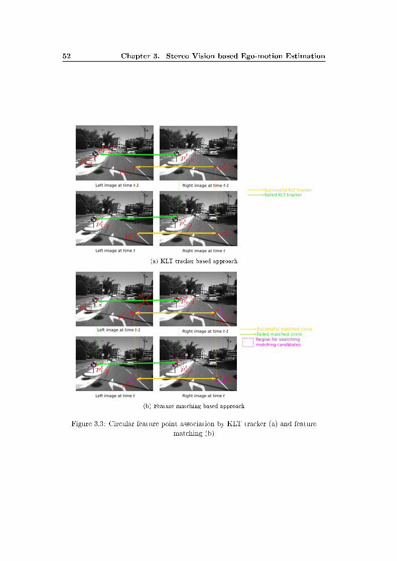
52 Chapter 3. Stereo Vision based Ego-motion Estimation
Left image at time t Right image at time t
Left image at time t-1 Right image at time t-1Successful KLT trackerFailed KLT tracker
(a) KLT tracker based approach
Left image at time t Right image at time t
Left image at time t-1 Right image at time t-1Successful matched circle
Failed matched circle
Region for searching
matching candidates
(b) Feature matching based approach
Figure 3.3: Circular feature point association by KLT tracker (a) and feature
matching (b)
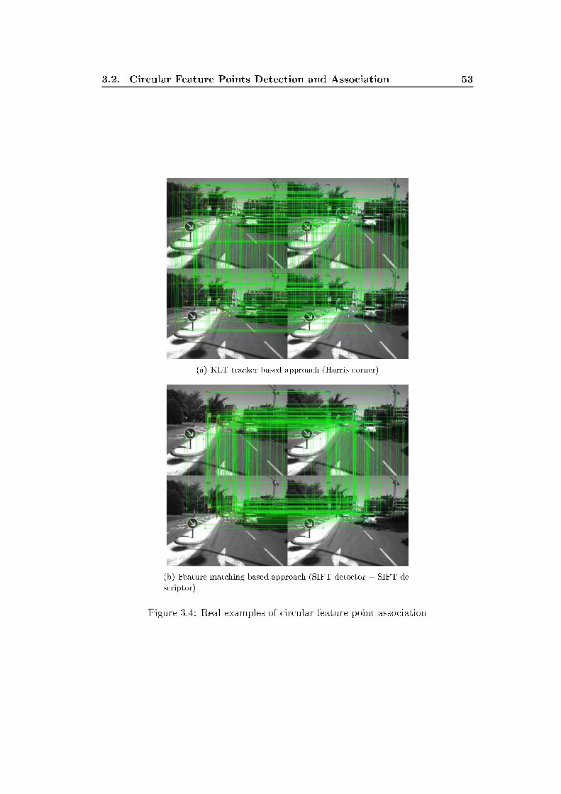
3.2. Circular Feature Points Detection and Association 53
(a) KLT tracker based approach (Harris corner)
(b) Feature matching based approach (SIFT detector + SIFT de-
scriptor)
Figure 3.4: Real examples of circular feature point association
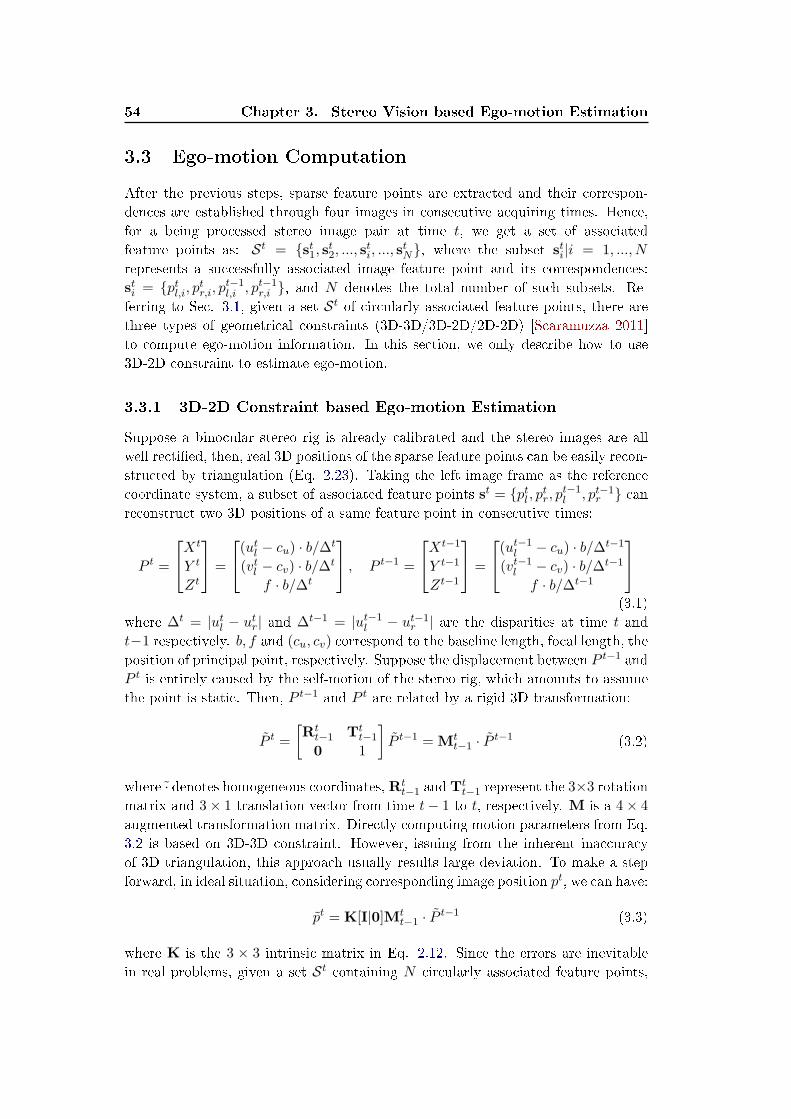
54 Chapter 3. Stereo Vision based Ego-motion Estimation
3.3 Ego-motion Computation
After the previous steps, sparse feature points are extracted and their correspon-
dences are established through four images in consecutive acquiring times. Hence,
for a being processed stereo image pair at time t, we get a set of associated
feature points as: St = {st1, st2, ..., sti, ..., stN}, where the subset sti|i = 1, ..., N
represents a successfully associated image feature point and its correspondences:
sti = {ptl,i, ptr,i, pt−1l,i , pt−1
r,i }, and N denotes the total number of such subsets. Re-
ferring to Sec. 3.1, given a set St of circularly associated feature points, there are
three types of geometrical constraints (3D-3D/3D-2D/2D-2D) [Scaramuzza 2011]
to compute ego-motion information. In this section, we only describe how to use
3D-2D constraint to estimate ego-motion.
3.3.1 3D-2D Constraint based Ego-motion Estimation
Suppose a binocular stereo rig is already calibrated and the stereo images are all
well recti�ed, then, real 3D positions of the sparse feature points can be easily recon-
structed by triangulation (Eq. 2.23). Taking the left image frame as the reference
coordinate system, a subset of associated feature points st = {ptl , ptr, pt−1l , pt−1
r } canreconstruct two 3D positions of a same feature point in consecutive times:
P t =
Xt
Y t
Zt
=
(utl − cu) · b/∆t
(vtl − cv) · b/∆t
f · b/∆t
, P t−1 =
Xt−1
Y t−1
Zt−1
=
(ut−1l − cu) · b/∆t−1
(vt−1l − cv) · b/∆t−1
f · b/∆t−1
(3.1)
where ∆t = |utl − utr| and ∆t−1 = |ut−1l − ut−1
r | are the disparities at time t and
t−1 respectively. b, f and (cu, cv) correspond to the baseline length, focal length, the
position of principal point, respectively. Suppose the displacement between P t−1 and
P t is entirely caused by the self-motion of the stereo rig, which amounts to assume
the point is static. Then, P t−1 and P t are related by a rigid 3D transformation:
P t =
[
Rtt−1 Tt
t−1
0 1
]
P t−1 = Mtt−1 · P t−1 (3.2)
where · denotes homogeneous coordinates,Rtt−1 andTt
t−1 represent the 3×3 rotationmatrix and 3× 1 translation vector from time t− 1 to t, respectively. M is a 4× 4
augmented transformation matrix. Directly computing motion parameters from Eq.
3.2 is based on 3D-3D constraint. However, issuing from the inherent inaccuracy
of 3D triangulation, this approach usually results large deviation. To make a step
forward, in ideal situation, considering corresponding image position pt, we can have:
pt = K[I|0]Mtt−1 · P t−1 (3.3)
where K is the 3 × 3 intrinsic matrix in Eq. 2.12. Since the errors are inevitable
in real problems, given a set St containing N circularly associated feature points,
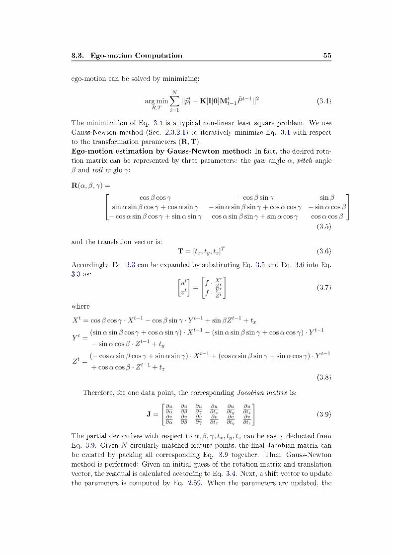
3.3. Ego-motion Computation 55
ego-motion can be solved by minimizing:
argminR,T
N∑
i=1
||ptl −K[I|0]Mtt−1P
t−1||2 (3.4)
The minimization of Eq. 3.4 is a typical non-linear least square problem. We use
Gauss-Newton method (Sec. 2.3.2.1) to iteratively minimize Eq. 3.4 with respect
to the transformation parameters (R,T).
Ego-motion estimation by Gauss-Newton method: In fact, the desired rota-
tion matrix can be represented by three parameters: the yaw angle α, pitch angle
β and roll angle γ:
R(α, β, γ) =
cosβ cos γ − cosβ sin γ sinβ
sinα sinβ cos γ + cosα sin γ − sinα sinβ sin γ + cosα cos γ − sinα cosβ
− cosα sinβ cos γ + sinα sin γ cosα sinβ sin γ + sinα cos γ cosα cosβ
(3.5)
and the translation vector is:
T = [tx, ty, tz]T (3.6)
Accordingly, Eq. 3.3 can be expanded by substituting Eq. 3.5 and Eq. 3.6 into Eq.
3.3 as:[
ut
vt
]
=
[
f · Xt
Zt
f · Y t
Zt
]
(3.7)
where
Xt = cosβ cos γ ·Xt−1 − cosβ sin γ · Y t−1 + sinβZt−1 + tx
Y t =(sinα sinβ cos γ + cosα sin γ) ·Xt−1 − (sinα sinβ sin γ + cosα cos γ) · Y t−1
− sinα cosβ · Zt−1 + ty
Zt =(− cosα sinβ cos γ + sinα sin γ) ·Xt−1 + (cosα sinβ sin γ + sinα cos γ) · Y t−1
+ cosα cosβ · Zt−1 + tz(3.8)
Therefore, for one data point, the corresponding Jacobian matrix is:
J =
[
∂u∂α
∂u∂β
∂u∂γ
∂u∂tx
∂u∂ty
∂u∂tz
∂v∂α
∂v∂β
∂v∂γ
∂v∂tx
∂v∂ty
∂v∂tz
]
(3.9)
The partial derivatives with respect to α, β, γ, tx, ty, tz can be easily deducted from
Eq. 3.9. Given N circularly matched feature points, the �nal Jacobian matrix can
be created by packing all corresponding Eq. 3.9 together. Then, Gauss-Newton
method is performed: Given an initial guess of the rotation matrix and translation
vector, the residual is calculated according to Eq. 3.4. Next, a shift vector to update
the parameters is computed by Eq. 2.59. When the parameters are updated, the
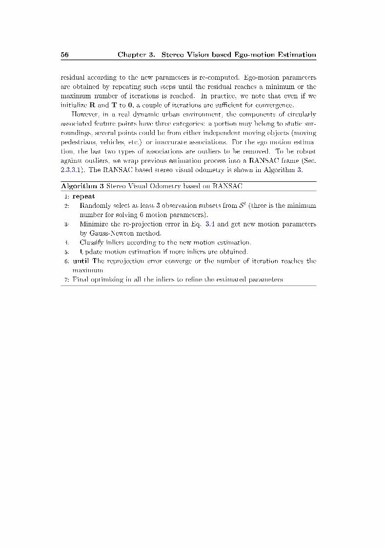
56 Chapter 3. Stereo Vision based Ego-motion Estimation
residual according to the new parameters is re-computed. Ego-motion parameters
are obtained by repeating such steps until the residual reaches a minimum or the
maximum number of iterations is reached. In practice, we note that even if we
initialize R and T to 0, a couple of iterations are su�cient for convergence.
However, in a real dynamic urban environment, the components of circularly
associated feature points have three categories: a portion may belong to static sur-
roundings, several points could be from either independent moving objects (moving
pedestrians, vehicles, etc.) or inaccurate associations. For the ego-motion estima-
tion, the last two types of associations are outliers to be removed. To be robust
against outliers, we wrap previous estimation process into a RANSAC frame (Sec.
2.3.3.1). The RANSAC based stereo visual odometry is shown in Algorithm 3.
Algorithm 3 Stereo Visual Odometry based on RANSAC
1: repeat2: Randomly select at least 3 observation subsets from St (three is the minimum
number for solving 6 motion parameters).
3: Minimize the re-projection error in Eq. 3.4 and get new motion parameters
by Gauss-Newton method.
4: Classify inliers according to the new motion estimation.
5: Update motion estimation if more inliers are obtained.
6: until The reprojection error converge or the number of iteration reaches the
maximum
7: Final optimizing in all the inliers to re�ne the estimated parameters
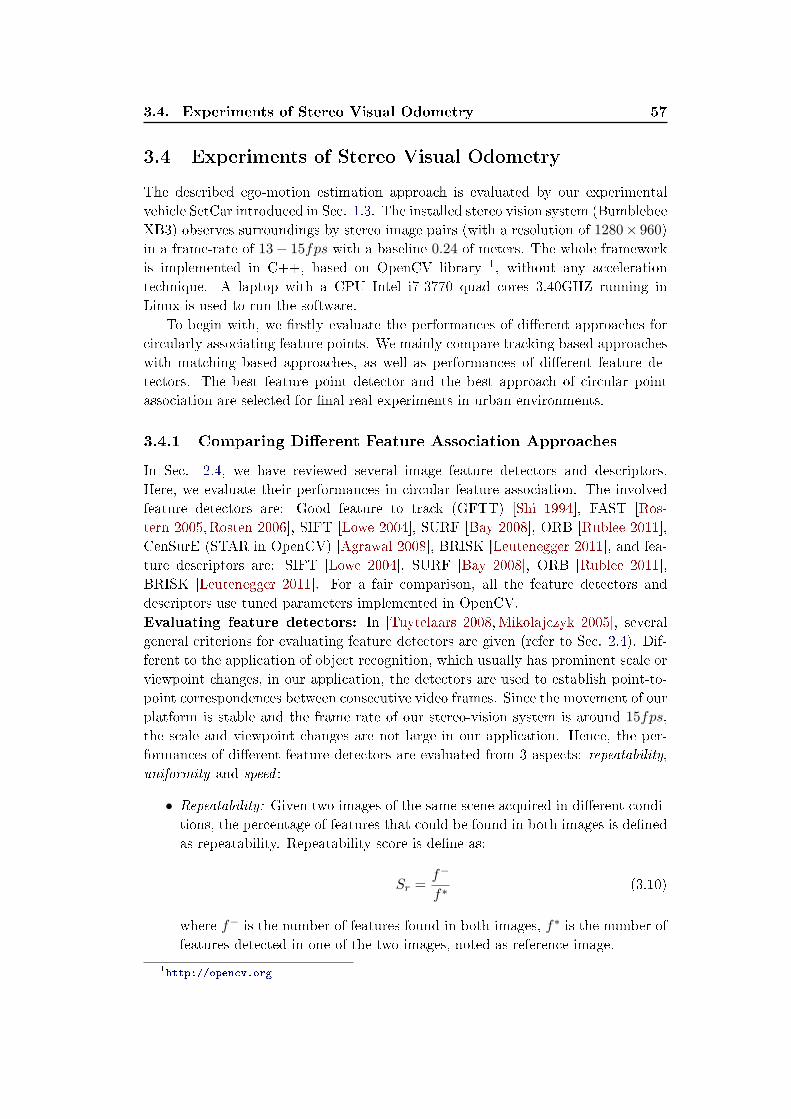
3.4. Experiments of Stereo Visual Odometry 57
3.4 Experiments of Stereo Visual Odometry
The described ego-motion estimation approach is evaluated by our experimental
vehicle SetCar introduced in Sec. 1.3. The installed stereo vision system (Bumblebee
XB3) observes surroundings by stereo image pairs (with a resolution of 1280× 960)
in a frame-rate of 13− 15fps with a baseline 0.24 of meters. The whole framework
is implemented in C++, based on OpenCV library 1, without any acceleration
technique. A laptop with a CPU Intel i7-3770 quad cores 3.40GHZ running in
Linux is used to run the software.
To begin with, we �rstly evaluate the performances of di�erent approaches for
circularly associating feature points. We mainly compare tracking based approaches
with matching based approaches, as well as performances of di�erent feature de-
tectors. The best feature point detector and the best approach of circular point
association are selected for �nal real experiments in urban environments.
3.4.1 Comparing Di�erent Feature Association Approaches
In Sec. 2.4, we have reviewed several image feature detectors and descriptors.
Here, we evaluate their performances in circular feature association. The involved
feature detectors are: Good feature to track (GFTT) [Shi 1994], FAST [Ros-
tern 2005,Rosten 2006], SIFT [Lowe 2004], SURF [Bay 2008], ORB [Rublee 2011],
CenSurE (STAR in OpenCV) [Agrawal 2008], BRISK [Leutenegger 2011], and fea-
ture descriptors are: SIFT [Lowe 2004], SURF [Bay 2008], ORB [Rublee 2011],
BRISK [Leutenegger 2011]. For a fair comparison, all the feature detectors and
descriptors use tuned parameters implemented in OpenCV.
Evaluating feature detectors: In [Tuytelaars 2008,Mikolajczyk 2005], several
general criterions for evaluating feature detectors are given (refer to Sec. 2.4). Dif-
ferent to the application of object recognition, which usually has prominent scale or
viewpoint changes, in our application, the detectors are used to establish point-to-
point correspondences between consecutive video frames. Since the movement of our
platform is stable and the frame rate of our stereo-vision system is around 15fps,
the scale and viewpoint changes are not large in our application. Hence, the per-
formances of di�erent feature detectors are evaluated from 3 aspects: repeatability,
uniformity and speed :
• Repeatability: Given two images of the same scene acquired in di�erent condi-
tions, the percentage of features that could be found in both images is de�ned
as repeatability. Repeatability score is de�ne as:
Sr =f−
f∗(3.10)
where f− is the number of features found in both images, f∗ is the number of
features detected in one of the two images, noted as reference image.
1http://opencv.org
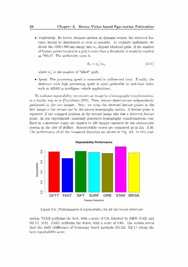
58 Chapter 3. Stereo Vision based Ego-motion Estimation
• Uniformity: To better estimate motion in dynamic scenes, the detected fea-
tures should be distributed as even as possible. To evaluate uniformity, we
divide the 1280 ∗ 960 size image into nu disjoint identical grids. If the number
of feature points located in a grid is more than a threshold, it would be marked
as "�lled". The uniformity score is:
Su = n−u /nu (3.11)
where n−u is the number of "�lled" grids.
• Speed: The processing speed is measured in millisecond (ms). Usually, the
detectors with high processing speed is more preferable in real-time tasks,
such as ADAS in intelligent vehicle applications.
To evaluate repeatability, we convert an image by a homography transformation,
in a similar way as in [Tuytelaars 2008]. Then, feature detectors are independently
performed in the two images. Next, we wrap the detected feature points in the
�rst image to the second one by the known homography matrix. A feature point is
repeated, if the wrapped position in the second image also has a detected feature
point. In our experiments, randomly generated homography transformations con-
�ned in a moderate range are applied to 100 images captured by our stereoscopic
system in the city of Belfort. Repeatability scores are computed as in Eq. 3.10.
The performance of all the measured detectors are shown in Fig. 3.5. In this eval-
GFTT FAST SIFT SURF ORB STAR BRISK
Repeatability Performance
Feature Detectors
Rep
eata
bilit
y
0.0
0.2
0.4
0.6
0.8
Figure 3.5: Performances of repeatability for all the tested detectors
uation, STAR performs the best, with a score of 0.9, followed by SIFT (0.82) and
GFTT (0.8). FAST performs the worst, with a score of 0.64. The results reveal
that the DoG (Di�erence of Gaussian) based methods (STAR, SIFT) attain the
best repeatability score.
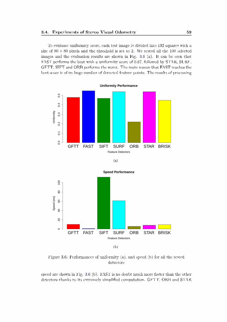
3.4. Experiments of Stereo Visual Odometry 59
To evaluate uniformity score, each test image is divided into 192 squares with a
size of 80 × 80 pixels and the threshold is set to 2. We tested all the 100 selected
images and the evaluation results are shown in Fig. 3.6 (a). It can be seen that
FAST performs the best with a uniformity score of 0.67, followed by STAR, SURF,
GFTT, SIFT and ORB performs the worst. The main reason that FAST reaches the
best score is of its huge number of detected feature points. The results of processing
GFTT FAST SIFT SURF ORB STAR BRISK
Uniformity Performance
Feature Detectors
Uni
form
ity
0.0
0.1
0.2
0.3
0.4
0.5
(a)
GFTT FAST SIFT SURF ORB STAR BRISK
Speed Performance
Feature Detectors
Spe
ed (
ms)
020
4060
8010
0
(b)
Figure 3.6: Performances of uniformity (a), and speed (b) for all the tested
detectors
speed are shown in Fig. 3.6 (b). FAST is no doubt much more faster than the other
detectors thanks to its extremely simpli�ed computation. GFTT, ORB and STAR
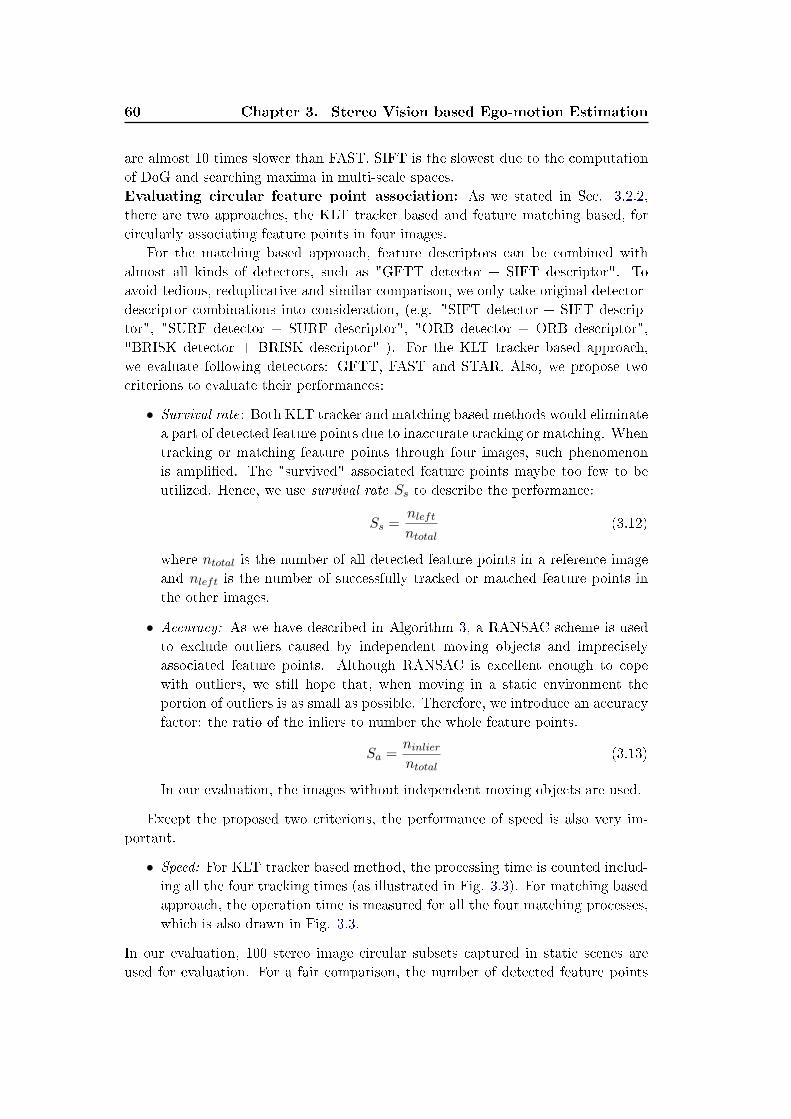
60 Chapter 3. Stereo Vision based Ego-motion Estimation
are almost 10 times slower than FAST. SIFT is the slowest due to the computation
of DoG and searching maxima in multi-scale spaces.
Evaluating circular feature point association: As we stated in Sec. 3.2.2,
there are two approaches, the KLT tracker based and feature matching based, for
circularly associating feature points in four images.
For the matching based approach, feature descriptors can be combined with
almost all kinds of detectors, such as "GFTT detector + SIFT descriptor". To
avoid tedious, reduplicative and similar comparison, we only take original detector-
descriptor combinations into consideration, (e.g. "SIFT detector + SIFT descrip-
tor", "SURF detector + SURF descriptor", "ORB detector + ORB descriptor",
"BRISK detector + BRISK descriptor" ). For the KLT tracker based approach,
we evaluate following detectors: GFTT, FAST and STAR. Also, we propose two
criterions to evaluate their performances:
• Survival rate: Both KLT tracker and matching based methods would eliminate
a part of detected feature points due to inaccurate tracking or matching. When
tracking or matching feature points through four images, such phenomenon
is ampli�ed. The "survived" associated feature points maybe too few to be
utilized. Hence, we use survival rate Ss to describe the performance:
Ss =nleft
ntotal(3.12)
where ntotal is the number of all detected feature points in a reference image
and nleft is the number of successfully tracked or matched feature points in
the other images.
• Accuracy: As we have described in Algorithm 3, a RANSAC scheme is used
to exclude outliers caused by independent moving objects and imprecisely
associated feature points. Although RANSAC is excellent enough to cope
with outliers, we still hope that, when moving in a static environment the
portion of outliers is as small as possible. Therefore, we introduce an accuracy
factor: the ratio of the inliers to number the whole feature points.
Sa =ninlier
ntotal(3.13)
In our evaluation, the images without independent moving objects are used.
Except the proposed two criterions, the performance of speed is also very im-
portant.
• Speed: For KLT tracker based method, the processing time is counted includ-
ing all the four tracking times (as illustrated in Fig. 3.3). For matching based
approach, the operation time is measured for all the four matching processes,
which is also drawn in Fig. 3.3.
In our evaluation, 100 stereo image circular subsets captured in static scenes are
used for evaluation. For a fair comparison, the number of detected feature points
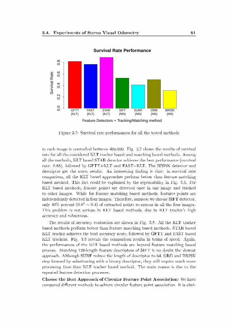
3.4. Experiments of Stereo Visual Odometry 61
GFTT(KLT)
FAST(KLT)
STAR(KLT)
SIFT(NN)
SURF(NN)
ORB(NN)
BRISK(NN)
Survival Rate Performance
Feature Detectors + Tracking/Matching method
Sur
viva
l Rat
e
0.0
0.2
0.4
0.6
0.8
Figure 3.7: Survival rate performances for all the tested methods
in each image is controlled between 400-500. Fig. 3.7 shows the results of survival
rate for all the considered KLT tracker based and matching based methods. Among
all the methods, KLT based STAR detector achieves the best performance (survival
rate: 0.88), followed by GFTT+KLT and FAST+KLT. The BRISK detector and
descriptor get the worst results. An interesting �nding is that: in survival rate
comparison, all the KLT based approaches perform better than feature matching
based method. This fact could be explained by the repeatability in Fig. 3.5. For
KLT based methods, feature points are detected once in one image and tracked
to other images. While for feature matching based methods, features points are
independently detected in four images. Therefore, suppose we choose SIFT detector,
only 40% percent (0.84 ∼ 0.4) of extracted points re-appear in all the four images.
This problem is not serious in KLT based methods, due to KLT tracker's high
accuracy and robustness.
The results of accuracy evaluation are shown in Fig. 3.8. All the KLT tracker
based methods perform better than feature matching based methods. STAR based
KLT tracker achieves the best accuracy score, followed by GFTT and FAST based
KLT trackers. Fig. 3.9 reveals the comparison results in terms of speed. Again,
the performances of the KLT based methods are beyond feature matching based
process. Matching 128-length feature descriptors of SIFT is no doubt the slowest
approach. Although SURF reduce the length of descriptor to 64, ORB and BRISK
step forward by substituting with a binary descriptor, they still require much more
processing time than KLT tracker based method. The main reason is due to the
repeated feature detection processes.
Choose the Best Approach of Circular Feature Point Association: We have
compared di�erent methods to achieve circular feature point association. It is obvi-
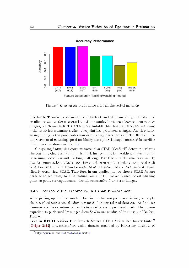
62 Chapter 3. Stereo Vision based Ego-motion Estimation
GFTT(KLT)
FAST(KLT)
STAR(KLT)
SIFT(NN)
SURF(NN)
ORB(NN)
BRISK(NN)
Accuracy Performance
Feature Detectors + Tracking/Matching method
Acc
urac
y
0.0
0.2
0.4
0.6
0.8
Figure 3.8: Accuracy performances for all the tested methods
ous that KLT tracker based methods are better than feature matching methods. The
results are due to the characteristic of unremarkable changes between consecutive
images, which makes KLT tracker more suitable than feature descriptor matching
� the latter has advantages when viewpoint has prominent changes. Another inter-
esting �nding is the poor performances of binary descriptors (ORB, BRISK). The
improvement of matching speed for binary descriptors is maybe obtained in sacri�ce
of accuracy, as shown in Fig. 3.8
Comparing feature detectors, we notice that STAR (CenSurE) detector performs
the best in global evaluation. It is quick for computation, stable and accurate for
cross-image detection and tracking. Although FAST feature detector is extremely
fast for computation, it lacks robustness and accuracy for tracking, compared with
STAR or GFTT. GFTT can be regarded as the second best choice, since it is just
slightly worse than STAR. Therefore, in our application, we choose STAR feature
detector to accurately localize feature points. KLT tracker is used for establishing
point-to-point correspondences through consecutive four stereo images.
3.4.2 Stereo Visual Odometry in Urban Environment
After picking up the best method for circular feature point association, we apply
the described stereo visual odometry method in several real datasets. At �rst, we
demonstrate the experimental results in a well-known open benchmark. Then, more
experiments performed by our platform SetCar are conducted in the city of Belfort,
France.
Test in KITTI Vision Benchmark Suite: KITTI Vision Benchmark Suite 2
[Geiger 2012] is a state-of-art vision dataset provided by Karlsruhe Institute of
2http://www.cvlibs.net/datasets/kitti/
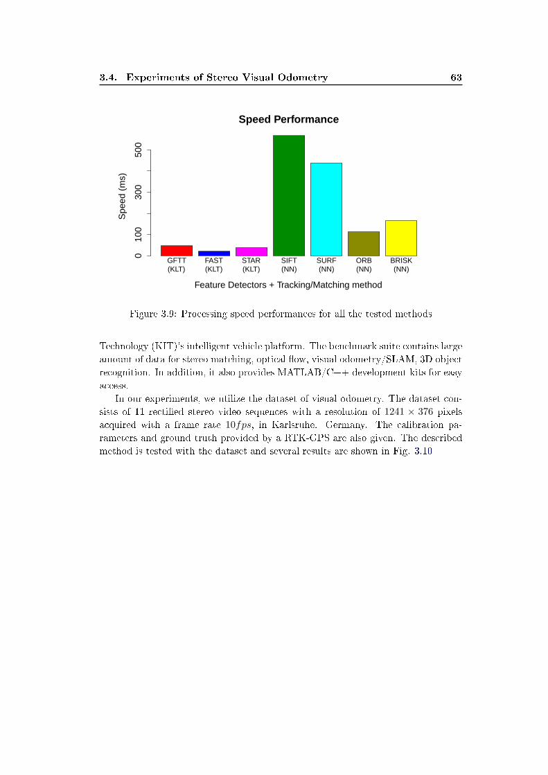
3.4. Experiments of Stereo Visual Odometry 63
GFTT(KLT)
FAST(KLT)
STAR(KLT)
SIFT(NN)
SURF(NN)
ORB(NN)
BRISK(NN)
Speed Performance
Feature Detectors + Tracking/Matching method
Spe
ed (
ms)
010
030
050
0
Figure 3.9: Processing speed performances for all the tested methods
Technology (KIT)'s intelligent vehicle platform. The benchmark suite contains large
amount of data for stereo matching, optical �ow, visual odometry/SLAM, 3D object
recognition. In addition, it also provides MATLAB/C++ development kits for easy
access.
In our experiments, we utilize the dataset of visual odometry. The dataset con-
sists of 11 recti�ed stereo video sequences with a resolution of 1241 × 376 pixels
acquired with a frame rate 10fps, in Karlsruhe. Germany. The calibration pa-
rameters and ground truth provided by a RTK-GPS are also given. The described
method is tested with the dataset and several results are shown in Fig. 3.10
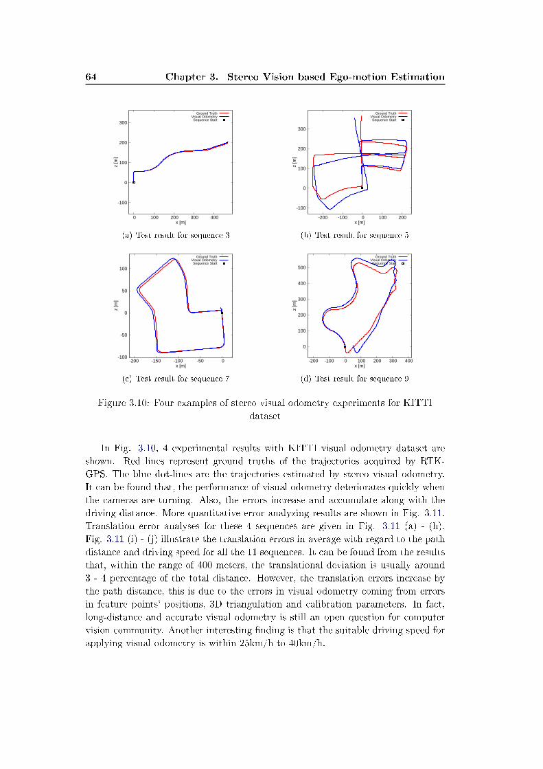
64 Chapter 3. Stereo Vision based Ego-motion Estimation
-100
0
100
200
300
0 100 200 300 400
z [m
]
x [m]
Ground TruthVisual OdometrySequence Start
(a) Test result for sequence 3
-100
0
100
200
300
-200 -100 0 100 200
z [m
]
x [m]
Ground TruthVisual OdometrySequence Start
(b) Test result for sequence 5
-100
-50
0
50
100
-200 -150 -100 -50 0
z [m
]
x [m]
Ground TruthVisual OdometrySequence Start
(c) Test result for sequence 7
0
100
200
300
400
500
-200 -100 0 100 200 300 400
z [m
]
x [m]
Ground TruthVisual OdometrySequence Start
(d) Test result for sequence 9
Figure 3.10: Four examples of stereo visual odometry experiments for KITTI
dataset
In Fig. 3.10, 4 experimental results with KITTI visual odometry dataset are
shown. Red lines represent ground truths of the trajectories acquired by RTK-
GPS. The blue dot-lines are the trajectories estimated by stereo visual odometry.
It can be found that, the performance of visual odometry deteriorates quickly when
the cameras are turning. Also, the errors increase and accumulate along with the
driving distance. More quantitative error analyzing results are shown in Fig. 3.11.
Translation error analyses for these 4 sequences are given in Fig. 3.11 (a) - (h).
Fig. 3.11 (i) - (j) illustrate the translation errors in average with regard to the path
distance and driving speed for all the 11 sequences. It can be found from the results
that, within the range of 400 meters, the translational deviation is usually around
3 - 4 percentage of the total distance. However, the translation errors increase by
the path distance, this is due to the errors in visual odometry coming from errors
in feature points' positions, 3D triangulation and calibration parameters. In fact,
long-distance and accurate visual odometry is still an open question for computer
vision community. Another interesting �nding is that the suitable driving speed for
applying visual odometry is within 25km/h to 40km/h.
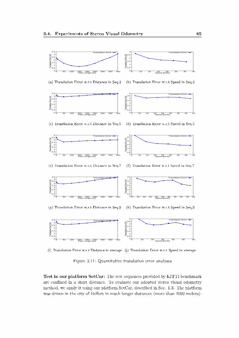
3.4. Experiments of Stereo Visual Odometry 65
0
0.5
1
1.5
2
2.5
3
3.5
0 50 100 150 200 250 300 350 400
Tran
slatio
n Erro
r [%]
Path Length [m]
Translation Error
(a) Translation Error w.r.t Distance in Seq.3
0
0.5
1
1.5
2
2.5
3
5 10 15 20 25 30 35 40
Tran
slatio
n Erro
r [%]
Speed [km/h]
Translation Error
(b) Translation Error w.r.t Speed in Seq.3
0
0.5
1
1.5
2
2.5
3
3.5
0 50 100 150 200 250 300 350 400
Tran
slatio
n Erro
r [%]
Path Length [m]
Translation Error
(c) Translation Error w.r.t Distance in Seq.5
0
0.5
1
1.5
2
2.5
3
3.5
4
5 10 15 20 25 30 35 40 45
Tran
slatio
n Erro
r [%]
Speed [km/h]
Translation Error
(d) Translation Error w.r.t Speed in Seq.5
0
0.5
1
1.5
2
2.5
3
3.5
4
0 50 100 150 200 250 300 350 400
Tran
slatio
n Erro
r [%]
Path Length [m]
Translation Error
(e) Translation Error w.r.t Distance in Seq.7
0 0.5
1 1.5
2 2.5
3 3.5
4 4.5
5
5 10 15 20 25 30 35 40 45
Tran
slatio
n Erro
r [%]
Speed [km/h]
Translation Error
(f) Translation Error w.r.t Speed in Seq.7
0 0.5
1 1.5
2 2.5
3 3.5
4 4.5
0 50 100 150 200 250 300 350 400
Tran
slatio
n Erro
r [%]
Path Length [m]
Translation Error
(g) Translation Error w.r.t Distance in Seq.9
0 0.5
1 1.5
2 2.5
3 3.5
4 4.5
10 15 20 25 30 35 40 45 50 55 60
Tran
slatio
n Erro
r [%]
Speed [km/h]
Translation Error
(h) Translation Error w.r.t Speed in Seq.9
0
0.5
1
1.5
2
2.5
3
3.5
0 50 100 150 200 250 300 350 400
Tran
slatio
n Erro
r [%]
Path Length [m]
Translation Error
(i) Translation Error w.r.t Distance in average
0
0.5
1
1.5
2
2.5
3
3.5
4
0 10 20 30 40 50 60
Tran
slatio
n Erro
r [%]
Speed [km/h]
Translation Error
(j) Translation Error w.r.t Speed in average
Figure 3.11: Quantitative translation error analyses
Test in our platform SetCar: The test sequences provided by KITTI benchmark
are con�ned in a short distance. To evaluate our adopted stereo visual odometry
method, we apply it using our platform SetCar, described in Sec. 1.3. The platform
was driven in the city of Belfort in much longer distances (more than 1000 meters).
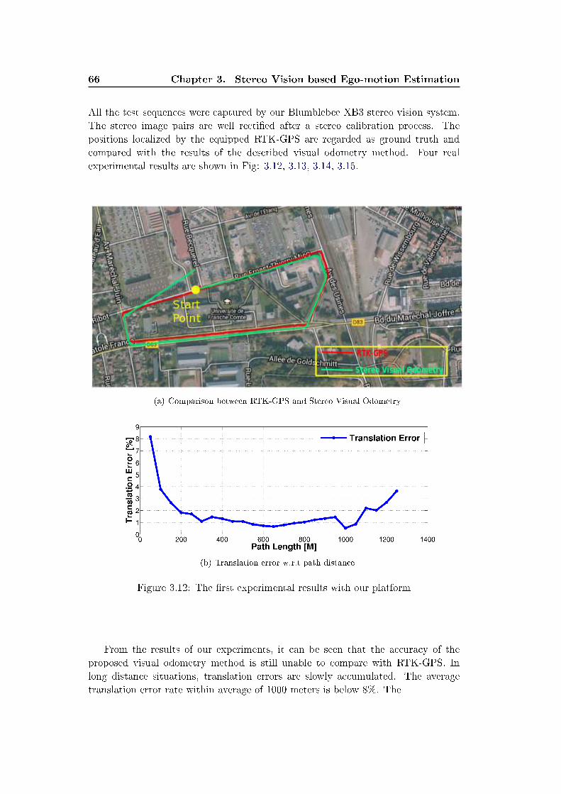
66 Chapter 3. Stereo Vision based Ego-motion Estimation
All the test sequences were captured by our Blumblebee XB3 stereo vision system.
The stereo image pairs are well recti�ed after a stereo calibration process. The
positions localized by the equipped RTK-GPS are regarded as ground truth and
compared with the results of the described visual odometry method. Four real
experimental results are shown in Fig: 3.12, 3.13, 3.14, 3.15.
(a) Comparison between RTK-GPS and Stereo Visual Odometry
(b) Translation error w.r.t path distance
Figure 3.12: The �rst experimental results with our platform
From the results of our experiments, it can be seen that the accuracy of the
proposed visual odometry method is still unable to compare with RTK-GPS. In
long distance situations, translation errors are slowly accumulated. The average
translation error rate within average of 1000 meters is below 8%. The
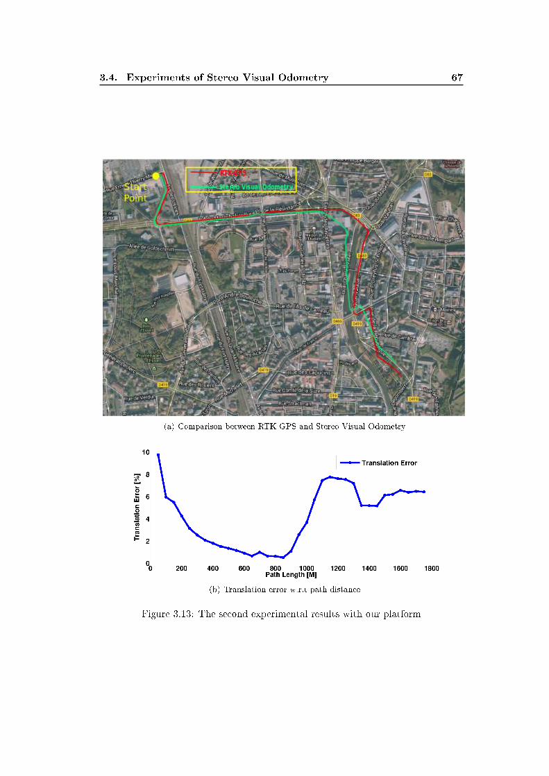
3.4. Experiments of Stereo Visual Odometry 67
(a) Comparison between RTK-GPS and Stereo Visual Odometry
(b) Translation error w.r.t path distance
Figure 3.13: The second experimental results with our platform
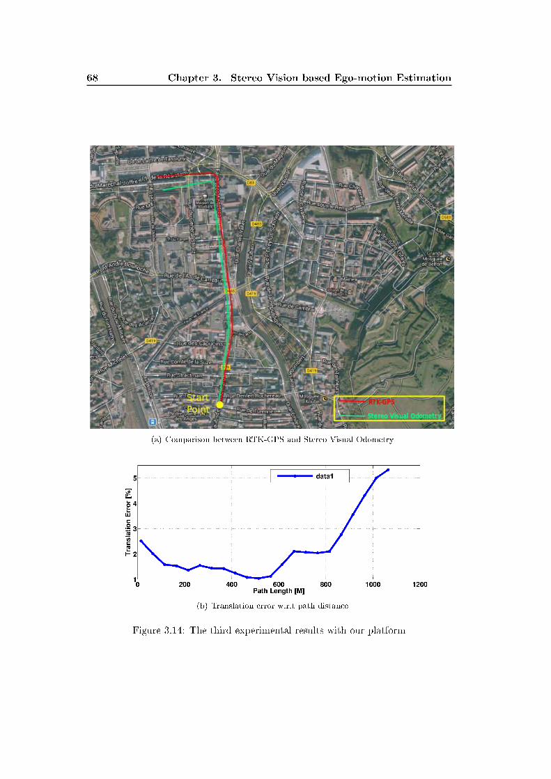
68 Chapter 3. Stereo Vision based Ego-motion Estimation
(a) Comparison between RTK-GPS and Stereo Visual Odometry
(b) Translation error w.r.t path distance
Figure 3.14: The third experimental results with our platform
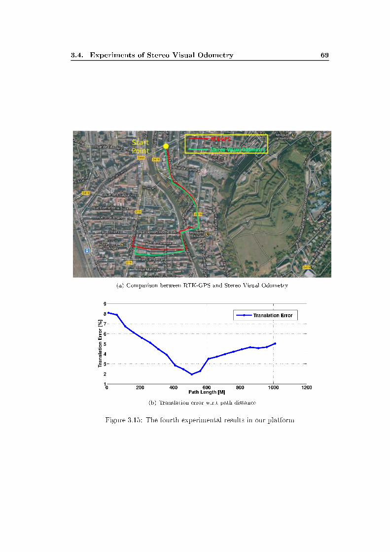
3.4. Experiments of Stereo Visual Odometry 69
(a) Comparison between RTK-GPS and Stereo Visual Odometry
(b) Translation error w.r.t path distance
Figure 3.15: The fourth experimental results in our platform
70 Chapter 3. Stereo Vision based Ego-motion Estimation
3.5 Conclusion and Future Works
In this chapter, we presented a stereo vision based method to estimate ego-motion
for a moving intelligent vehicle. The ego-motion information of the vehicle itself
(visual odometry) is �rstly investigated by utilizing quad-associated feature points
in consecutive stereo images. To improve the accuracy of visual odometry, various
image features and methods of feature association are tested and compared. The ex-
perimental comparisons showed that the combination of CenSurE and KLT tracker
achieves the best performance. Real experiments of visual odometry are tested with
an open benchmark, as well as our platform. From the experiments, we can see
that, compared with RTK-GPS, visual odometry still lacks of accuracy. The future
works would focus on improving accuracy of visual odometry.
To improve the accuracy of feature based visual odometry, following approaches
could be attempted:
• Improve the accuracy of key points locations by computing sub-pixel posi-
tions. In our experiments, the positions of feature points are in discretized
coordinates. However, real world is continues. The usage of sub-pixel position
of feature points maybe increase the accuracy of visual odometry.
• Model the error of key points locations. In our experiments, the weights
of all feature points are the same. Modeling the error of di�erent key points
according to distance or other criterions maybe improve the accuracy of stereo
visual odometry.
Chapter 4
Independent Moving Object
Detection, Segmentation and
Recognition
Contents
4.1 Independent Moving Object Detection and Segmentation . 71
4.1.1 Introduction . . . . . . . . . . . . . . . . . . . . . . . . . . . 71
4.1.2 UV-Disparity Based Independent Moving Objectxs Detection
and Segmentation . . . . . . . . . . . . . . . . . . . . . . . . 73
4.1.3 Experimental results of U-disparity image based Independent
Moving Object Detection . . . . . . . . . . . . . . . . . . . . 77
4.2 Moving Object Recognition using Spatial Information . . . 80
4.2.1 Introduction . . . . . . . . . . . . . . . . . . . . . . . . . . . 80
4.2.2 Spatial Feature Extraction and Classi�cation . . . . . . . . . 81
4.2.3 Experimental Results . . . . . . . . . . . . . . . . . . . . . . 84
4.3 Conclusion and Future Works . . . . . . . . . . . . . . . . . . 89
In the previous chapter, we presented a method of estimating ego-motion in-
formation for a moving intelligent vehicle. However, real urban environments are
complex in full of independent moving objects, such as moving pedestrians, vehicles,
cyclists, etc. Therefore, the perception system of an intelligent vehicle requires an
ability to analyze the moving objects when it is driven. In this chapter, we �rstly
present a method to detect and segment moving objects from moving stereo vision
system and then, we introduce a recognition method to recognize the segmented
objects based on spatial information.
4.1 Independent Moving Object Detection and Segmen-
tation
4.1.1 Introduction
Vision based moving object detection is an old but still dynamic computer vision
area. It provides a classi�cation of the pixels in video sequence into either foreground
(moving objects) or background. When the camera, or vision system, is static, one of
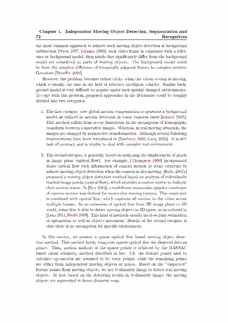
72Chapter 4. Independent Moving Object Detection, Segmentation and
Recognition
the most common approach to achieve such moving object detection is background
subtraction [Wren 1997,Toyama 1999]: each video frame is compared with a refer-
ence or background model, then pixels that signi�cantly di�er from the background
model are considered as parts of moving objects. The background model could
be from the simplest di�erence of temporally adjacent frames to complex mixture
Gaussians [Stau�er 2000].
However, the problem becomes rather tricky when the vision system is moving,
which is usually the case in the �eld of robotics, intelligent vehicles. Similar back-
ground model is very di�cult to acquire under such quickly changed environments.
To cope with this problem, proposed approaches in the litterature could be roughly
divided into two categories.
1. The �rst category uses global motion compensation to generate a background
model as utilized in motion detection in static cameras cases [Kaucic 2005].
This method su�ers from severe limitations in the assumption of homography
transform between consecutive images. Whereas, in real moving situation, the
images are changed by perspective transformation. Although several following
improvements have been introduced in [Sawhney 2000,Kang 2005]. It is still
lack of accuracy and is unable to deal with complex real environment.
2. The second category is generally based on analyzing the displacement of pixels
in image plane (optical �ow). For example, [Thompson 1990] incorporated
dense optical �ow with information of camera motion or scene structure to
achieve moving object detection when the camera is also moving. [Rabe 2007a]
proposed a moving object detection method based on analysis of individually
tracked image points (optical �ow), which provides a motion metric to indicate
their motion status. In [Dey 2012], a multiframe monocular epipolar constraint
of camera motion was derived for monocular moving camera. This constraint
is combined with optical �ow, which captures all motion in the video across
multiple frames. As an extension of optical �ow from 2D image plane to 3D
world, scene �ow is able to detect moving objects in 3D space, as introduced in
[Lenz 2011,Wedel 2009]. This kind of methods usually involves joint estimation
of ego-motion as well as objects movement. Bene�t of the second category is
that there is no assumption for speci�c environment.
In this section, we present a sparse optical �ow based moving object detec-
tion method. This method �rstly computes sparse optical �ow for detected feature
points. Then, motion analysis of the sparse points is achieved by the RANSAC
based visual odometry method described in Sec. 3.3: the feature points used to
calculate ego-motion are assumed to be static points, while the remaining points
are either from independent moving objects or noises. Based on the "suspected"
feature points from moving objects, we use U-disparity image to detect real moving
objects. At last, based on the detecting results in U-disparity image, the moving
objects are segmented in dense disparity map.
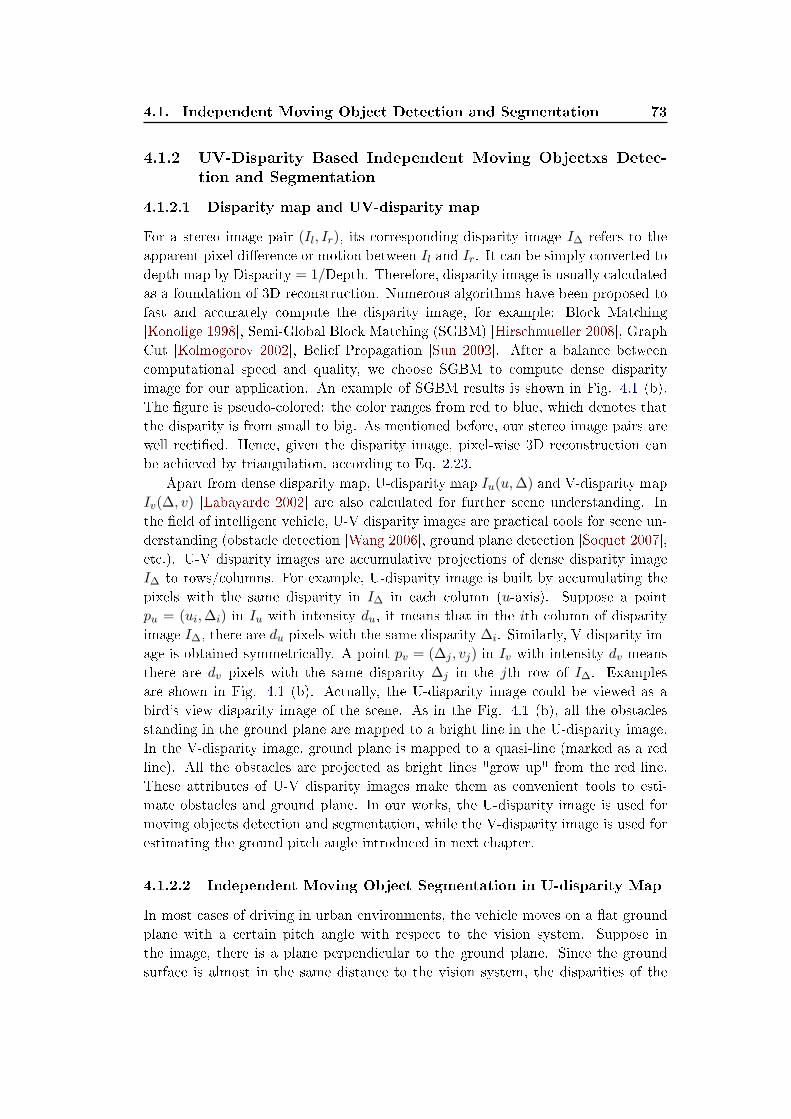
4.1. Independent Moving Object Detection and Segmentation 73
4.1.2 UV-Disparity Based Independent Moving Objectxs Detec-
tion and Segmentation
4.1.2.1 Disparity map and UV-disparity map
For a stereo image pair (Il, Ir), its corresponding disparity image I∆ refers to the
apparent pixel di�erence or motion between Il and Ir. It can be simply converted to
depth map by Disparity = 1/Depth. Therefore, disparity image is usually calculated
as a foundation of 3D reconstruction. Numerous algorithms have been proposed to
fast and accurately compute the disparity image, for example: Block Matching
[Konolige 1998], Semi-Global Block Matching (SGBM) [Hirschmueller 2008], Graph
Cut [Kolmogorov 2002], Belief Propagation [Sun 2002]. After a balance between
computational speed and quality, we choose SGBM to compute dense disparity
image for our application. An example of SGBM results is shown in Fig. 4.1 (b).
The �gure is pseudo-colored: the color ranges from red to blue, which denotes that
the disparity is from small to big. As mentioned before, our stereo image pairs are
well recti�ed. Hence, given the disparity image, pixel-wise 3D reconstruction can
be achieved by triangulation, according to Eq. 2.23.
Apart from dense disparity map, U-disparity map Iu(u,∆) and V-disparity map
Iv(∆, v) [Labayarde 2002] are also calculated for further scene understanding. In
the �eld of intelligent vehicle, U-V disparity images are practical tools for scene un-
derstanding (obstacle detection [Wang 2006], ground plane detection [Soquet 2007],
etc.). U-V disparity images are accumulative projections of dense disparity image
I∆ to rows/columns. For example, U-disparity image is built by accumulating the
pixels with the same disparity in I∆ in each column (u-axis). Suppose a point
pu = (ui,∆i) in Iu with intensity du, it means that in the ith column of disparity
image I∆, there are du pixels with the same disparity ∆i. Similarly, V-disparity im-
age is obtained symmetrically. A point pv = (∆j , vj) in Iv with intensity dv means
there are dv pixels with the same disparity ∆j in the jth row of I∆. Examples
are shown in Fig. 4.1 (b). Actually, the U-disparity image could be viewed as a
bird's view disparity image of the scene. As in the Fig. 4.1 (b), all the obstacles
standing in the ground plane are mapped to a bright line in the U-disparity image.
In the V-disparity image, ground plane is mapped to a quasi-line (marked as a red
line). All the obstacles are projected as bright lines "grow up" from the red line.
These attributes of U-V disparity images make them as convenient tools to esti-
mate obstacles and ground plane. In our works, the U-disparity image is used for
moving objects detection and segmentation, while the V-disparity image is used for
estimating the ground pitch angle introduced in next chapter.
4.1.2.2 Independent Moving Object Segmentation in U-disparity Map
In most cases of driving in urban environments, the vehicle moves on a �at ground
plane with a certain pitch angle with respect to the vision system. Suppose in
the image, there is a plane perpendicular to the ground plane. Since the ground
surface is almost in the same distance to the vision system, the disparities of the
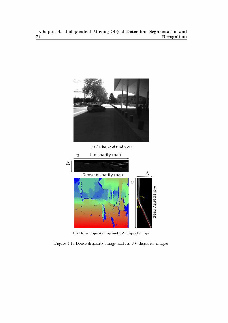
74Chapter 4. Independent Moving Object Detection, Segmentation and
Recognition
(a) An image of road scene
U-disparity map
V-d
isparity
map
Dense disparity map
(b) Dense disparity map and U-V disparity maps
Figure 4.1: Dense disparity image and its UV-disparity images
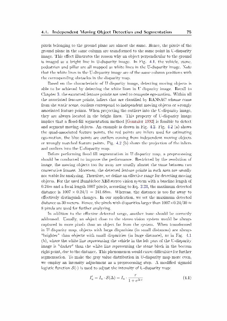
4.1. Independent Moving Object Detection and Segmentation 75
pixels belonging to the ground plane are almost the same. Hence, the pixels of the
ground plane in the same column are transformed to the same point in U-disparity
image. This e�ect illustrates the reason why an object perpendicular to the ground
is imaged as a bright line in U-disparity image. In Fig. 4.1, the vehicle, stone,
pedestrian and pillar are all mapped as white lines in the U-disparity image. Note
that the white lines in the U-disparity image are of the same column positions with
the corresponding obstacles in the disparity map.
Based on the characteristic of U-disparity image, detecting moving objects is
able to be achieved by detecting the white lines in U-disparity image. Recall to
Chapter 3, the extracted feature points are used to compute ego-motion. Within all
the associated feature points, inliers that are classi�ed by RANSAC scheme come
from the static scene, outliers correspond to independent moving objects or wrongly
associated feature points. When projecting the outliers into the U-disparity image,
they are always located in the bright lines. This property of U-disparity image
implies that a �ood-�ll segmentation method [Gonzalez 1992] is feasible to detect
and segment moving objects. An example is drawn in Fig. 4.2. Fig. 4.2 (a) shows
the quad-associated feature points, the red points are inliers used for estimating
ego-motion, the blue points are outliers coming from independent moving objects
or wrongly matched feature points. Fig. 4.2 (b) shows the projection of the inliers
and outliers into the U-disparity map.
Before performing �ood-�ll segmentation in U-disparity map, a preprocessing
should be conducted to improve the performance. Restricted by the resolution of
image, the moving objects too far away are usually almost the same between two
consecutive frames. Moreover, the detected feature points in such area are usually
not stable for analyzing. Therefore, we de�ne an e�ective range for detecting moving
objects. For the used Bumblebee XB3 stereo vision system with a baseline length of
0.24m and a focal length 1007 pixels, according to Eq. 2.23, the maximum detected
distance is 1007 × 0.24/1 = 241.68m. Whereas, the distance is too far away to
e�ectively distinguish changes. In our application, we set the maximum detected
distance as 30meters. Hence, the pixels with disparities larger than 1007×0.24/30 ≈8 pixels are used for further analyzing.
In addition to the e�ective detected range, another issue should be correctly
addressed. Usually, an object close to the stereo-vision system would be always
captured in more pixels than an object far from the system. When transformed
in U-disparity map, objects with large disparities (in small distances) are always
"brighter" than objects with small disparities (in large distance), as in Fig. 4.1
(b), where the white line representing the vehicle in the left part of the U-disparity
image is "darker" than the white line representing the stone block in the bottom
right point, due to the distance. This phenomenon would cause di�culties for further
segmentation. To make the gray value distribution in U-disparity map more even,
we employ an intensity adjustment as a preprocessing step. A modi�ed sigmoid
logistic function S(·) is used to adjust the intensity of U-disparity map:
I ′u = Iu · S(∆) = Iu ·r
1 + e∆·c(4.1)
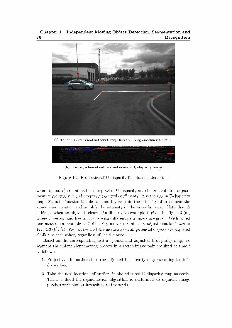
76Chapter 4. Independent Moving Object Detection, Segmentation and
Recognition
(a) The inliers (red) and outliers (blue) classi�ed by ego-motion estimation
(b) The projection of outliers and inliers in U-disparity image
Figure 4.2: Properties of U-disparity for obstacle detection
where Iu and I ′u are intensities of a pixel in U-disparity map before and after adjust-
ment, respectively. r and c represent control coe�cients. ∆ is the row in U-disparity
map. Sigmoid function is able to smoothly restrain the intensity of areas near the
stereo vision system and amplify the intensity of the areas far away. Note that ∆
is bigger when an object is closer. An illustrative example is given in Fig. 4.3 (a),
where three sigmoid-like functions with di�erent parameters are given. With tuned
parameters, an example of U-disparity map after intensity adjustment is shown in
Fig. 4.3 (b), (c). We can see that the intensities of all potential objects are adjusted
similar to each other, regardless of the distance.
Based on the corresponding feature points and adjusted U-disparity map, we
segment the independent moving objects in a stereo image pair acquired at time t
as follows:
1. Project all the outliers into the adjusted U-disparity map according to their
disparities.
2. Take the new locations of outliers in the adjusted U-disparity map as seeds.
Then, a �ood �ll segmentation algorithm is performed to segment image
patches with similar intensities to the seeds.
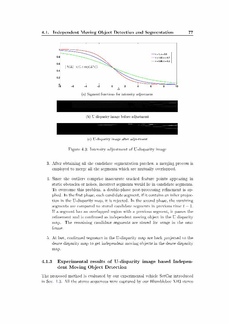
4.1. Independent Moving Object Detection and Segmentation 77
(a) Sigmoid functions for intensity adjustment
(b) U-disparity image before adjustment
(c) U-disparity image after adjustment
Figure 4.3: Intensity adjustment of U-disparity image
3. After obtaining all the candidate segmentation patches, a merging process is
employed to merge all the segments which are mutually overlapped.
4. Since the outliers comprise inaccurate tracked feature points appearing in
static obstacles or noises, incorrect segments would lie in candidate segments.
To overcome this problem, a double-phase post-processing re�nement is ap-
plied. In the �rst phase, each candidate segment, if it contains an inlier projec-
tion in the U-disparity map, it is rejected. In the second phase, the surviving
segments are compared to stored candidate segments in previous time t − 1.
If a segment has an overlapped region with a previous segment, it passes the
re�nement and is con�rmed as independent moving object in the U-disparity
map. The remaining candidate segments are stored for usage in the next
frame.
5. At last, con�rmed segments in the U-disparity map are back projected to the
dense disparity map to get independent moving objects in the dense disparity
map.
4.1.3 Experimental results of U-disparity image based Indepen-
dent Moving Object Detection
The proposed method is evaluated by our experimental vehicle SetCar introduced
in Sec. 1.3. All the stereo sequences were captured by our Blumblebee XB3 stereo
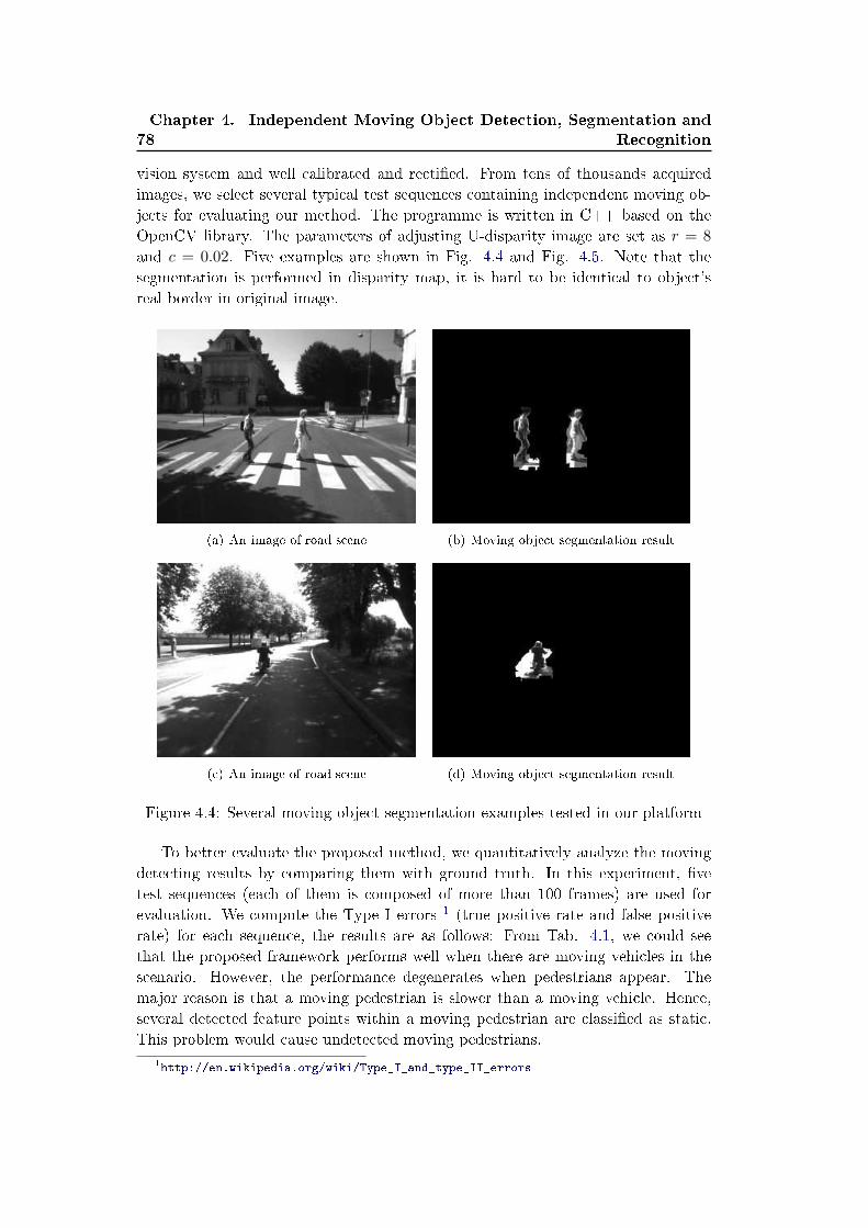
78Chapter 4. Independent Moving Object Detection, Segmentation and
Recognition
vision system and well calibrated and recti�ed. From tens of thousands acquired
images, we select several typical test sequences containing independent moving ob-
jects for evaluating our method. The programme is written in C++ based on the
OpenCV library. The parameters of adjusting U-disparity image are set as r = 8
and c = 0.02. Five examples are shown in Fig. 4.4 and Fig. 4.5. Note that the
segmentation is performed in disparity map, it is hard to be identical to object's
real border in original image.
(a) An image of road scene (b) Moving object segmentation result
(c) An image of road scene (d) Moving object segmentation result
Figure 4.4: Several moving object segmentation examples tested in our platform
To better evaluate the proposed method, we quantitatively analyze the moving
detecting results by comparing them with ground truth. In this experiment, �ve
test sequences (each of them is composed of more than 100 frames) are used for
evaluation. We compute the Type I errors 1 (true positive rate and false positive
rate) for each sequence, the results are as follows: From Tab. 4.1, we could see
that the proposed framework performs well when there are moving vehicles in the
scenario. However, the performance degenerates when pedestrians appear. The
major reason is that a moving pedestrian is slower than a moving vehicle. Hence,
several detected feature points within a moving pedestrian are classi�ed as static.
This problem would cause undetected moving pedestrians.
1http://en.wikipedia.org/wiki/Type_I_and_type_II_errors
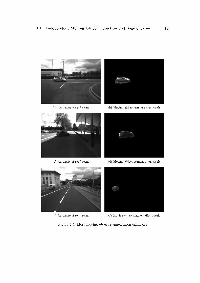
4.1. Independent Moving Object Detection and Segmentation 79
(a) An image of road scene (b) Moving object segmentation result
(c) An image of road scene (d) Moving object segmentation result
(e) An image of road scene (f) Moving object segmentation result
Figure 4.5: More moving object segmentation examples
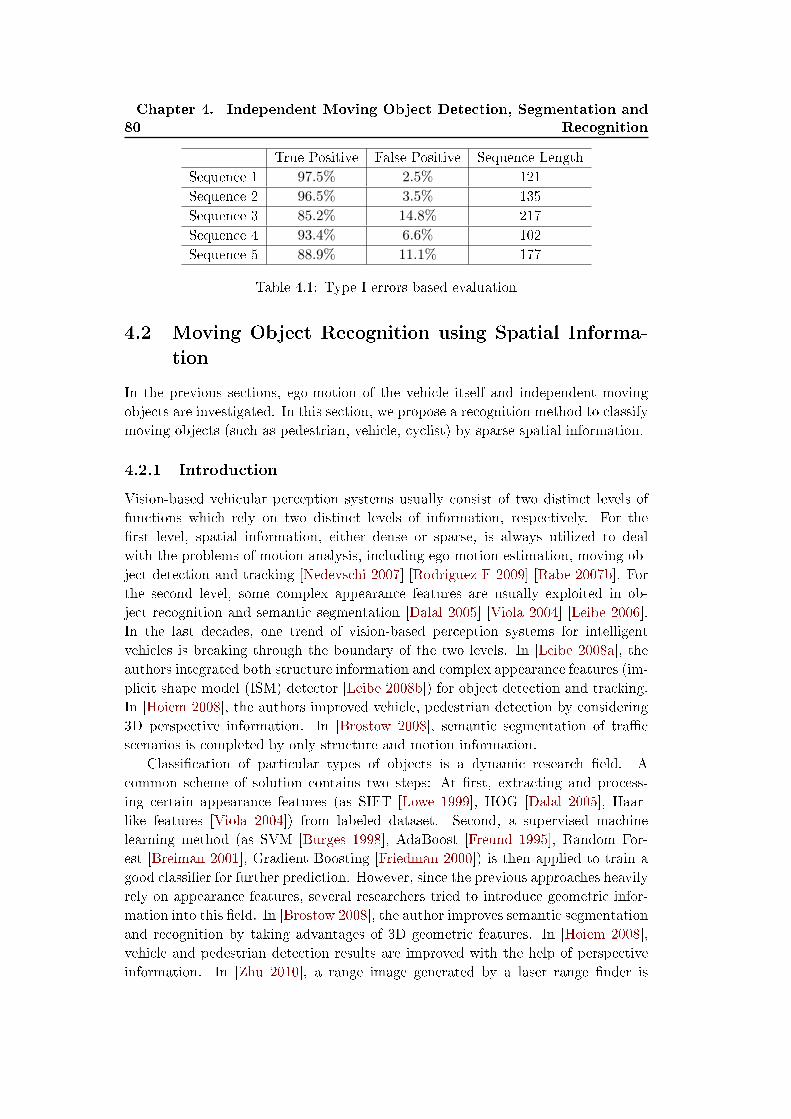
80Chapter 4. Independent Moving Object Detection, Segmentation and
Recognition
True Positive False Positive Sequence Length
Sequence 1 97.5% 2.5% 121
Sequence 2 96.5% 3.5% 135
Sequence 3 85.2% 14.8% 217
Sequence 4 93.4% 6.6% 102
Sequence 5 88.9% 11.1% 177
Table 4.1: Type I errors based evaluation
4.2 Moving Object Recognition using Spatial Informa-
tion
In the previous sections, ego-motion of the vehicle itself and independent moving
objects are investigated. In this section, we propose a recognition method to classify
moving objects (such as pedestrian, vehicle, cyclist) by sparse spatial information.
4.2.1 Introduction
Vision-based vehicular perception systems usually consist of two distinct levels of
functions which rely on two distinct levels of information, respectively. For the
�rst level, spatial information, either dense or sparse, is always utilized to deal
with the problems of motion analysis, including ego-motion estimation, moving ob-
ject detection and tracking [Nedevschi 2007] [Rodriguez F 2009] [Rabe 2007b]. For
the second level, some complex appearance features are usually exploited in ob-
ject recognition and semantic segmentation [Dalal 2005] [Viola 2004] [Leibe 2006].
In the last decades, one trend of vision-based perception systems for intelligent
vehicles is breaking through the boundary of the two levels. In [Leibe 2008a], the
authors integrated both structure information and complex appearance features (im-
plicit shape model (ISM) detector [Leibe 2008b]) for object detection and tracking.
In [Hoiem 2008], the authors improved vehicle, pedestrian detection by considering
3D perspective information. In [Brostow 2008], semantic segmentation of tra�c
scenarios is completed by only structure and motion information.
Classi�cation of particular types of objects is a dynamic research �eld. A
common scheme of solution contains two steps: At �rst, extracting and process-
ing certain appearance features (as SIFT [Lowe 1999], HOG [Dalal 2005], Haar-
like features [Viola 2004]) from labeled dataset. Second, a supervised machine
learning method (as SVM [Burges 1998], AdaBoost [Freund 1995], Random For-
est [Breiman 2001], Gradient Boosting [Friedman 2000]) is then applied to train a
good classi�er for further prediction. However, since the previous approaches heavily
rely on appearance features, several researchers tried to introduce geometric infor-
mation into this �eld. In [Brostow 2008], the author improves semantic segmentation
and recognition by taking advantages of 3D geometric features. In [Hoiem 2008],
vehicle and pedestrian detection results are improved with the help of perspective
information. In [Zhu 2010], a range image generated by a laser range �nder is
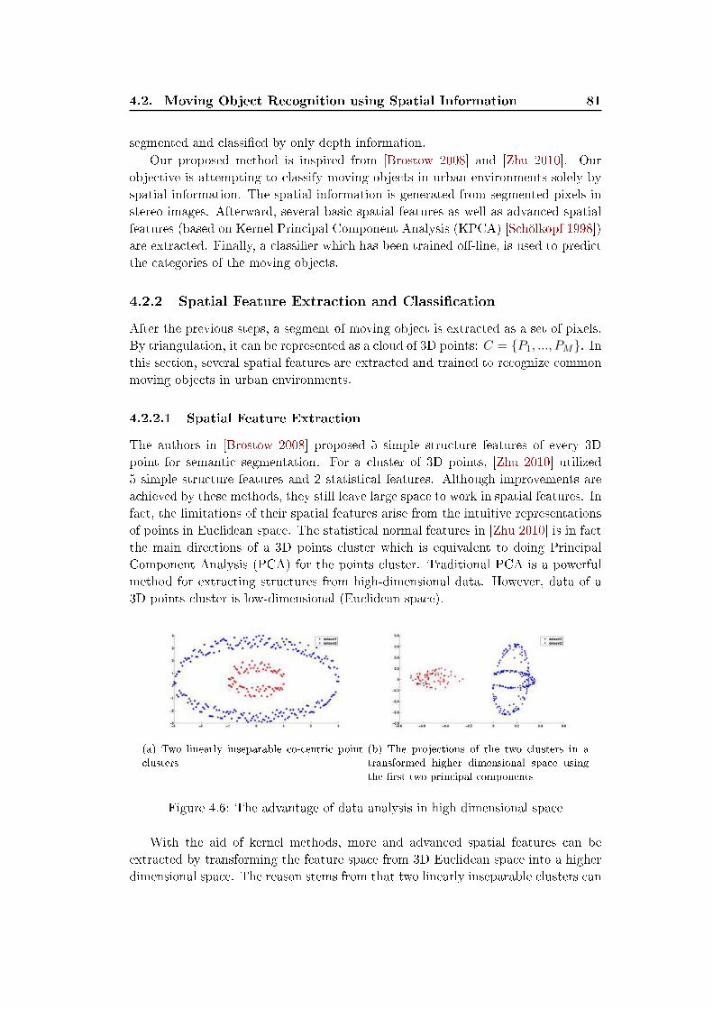
4.2. Moving Object Recognition using Spatial Information 81
segmented and classi�ed by only depth information.
Our proposed method is inspired from [Brostow 2008] and [Zhu 2010]. Our
objective is attempting to classify moving objects in urban environments solely by
spatial information. The spatial information is generated from segmented pixels in
stereo images. Afterward, several basic spatial features as well as advanced spatial
features (based on Kernel Principal Component Analysis (KPCA) [Schölkopf 1998])
are extracted. Finally, a classi�er which has been trained o�-line, is used to predict
the categories of the moving objects.
4.2.2 Spatial Feature Extraction and Classi�cation
After the previous steps, a segment of moving object is extracted as a set of pixels.
By triangulation, it can be represented as a cloud of 3D points: C = {P1, ..., PM}. Inthis section, several spatial features are extracted and trained to recognize common
moving objects in urban environments.
4.2.2.1 Spatial Feature Extraction
The authors in [Brostow 2008] proposed 5 simple structure features of every 3D
point for semantic segmentation. For a cluster of 3D points, [Zhu 2010] utilized
5 simple structure features and 2 statistical features. Although improvements are
achieved by these methods, they still leave large space to work in spatial features. In
fact, the limitations of their spatial features arise from the intuitive representations
of points in Euclidean space. The statistical normal features in [Zhu 2010] is in fact
the main directions of a 3D points cluster which is equivalent to doing Principal
Component Analysis (PCA) for the points cluster. Traditional PCA is a powerful
method for extracting structures from high-dimensional data. However, data of a
3D points cluster is low-dimensional (Euclidean space).
(a) Two linearly inseparable co-centric point
clusters
(b) The projections of the two clusters in a
transformed higher dimensional space using
the �rst two principal components
Figure 4.6: The advantage of data analysis in high dimensional space
With the aid of kernel methods, more and advanced spatial features can be
extracted by transforming the feature space from 3D Euclidean space into a higher
dimensional space. The reason stems from that two linearly inseparable clusters can
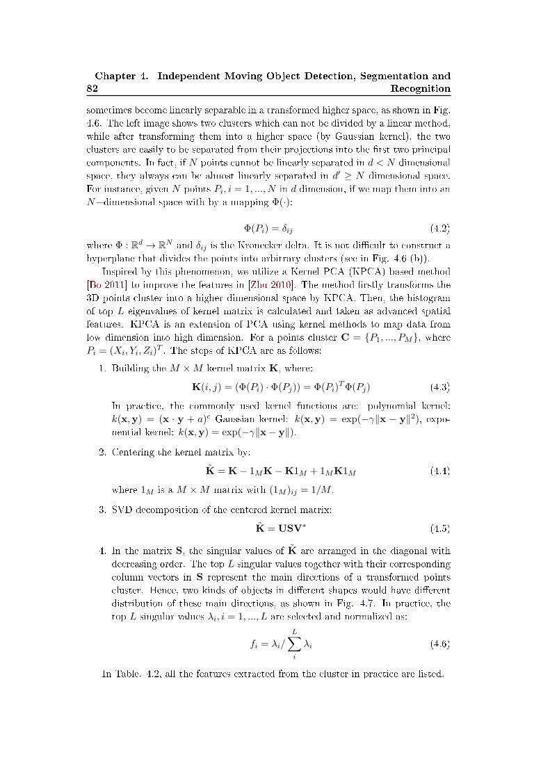
82Chapter 4. Independent Moving Object Detection, Segmentation and
Recognition
sometimes become linearly separable in a transformed higher space, as shown in Fig.
4.6. The left image shows two clusters which can not be divided by a linear method,
while after transforming them into a higher space (by Gaussian kernel), the two
clusters are easily to be separated from their projections into the �rst two principal
components. In fact, if N points cannot be linearly separated in d < N dimensional
space, they always can be almost linearly separated in d′ ≥ N dimensional space.
For instance, given N points Pi, i = 1, ..., N in d dimension, if we map them into an
N−dimensional space with by a mapping Φ(·):
Φ(Pi) = δij (4.2)
where Φ : Rd → RN and δij is the Kronecker delta. It is not di�cult to construct a
hyperplane that divides the points into arbitrary clusters (see in Fig. 4.6 (b)).
Inspired by this phenomenon, we utilize a Kernel PCA (KPCA) based method
[Bo 2011] to improve the features in [Zhu 2010]. The method �rstly transforms the
3D points cluster into a higher dimensional space by KPCA. Then, the histogram
of top L eigenvalues of kernel matrix is calculated and taken as advanced spatial
features. KPCA is an extension of PCA using kernel methods to map data from
low dimension into high dimension. For a points cluster C = {P1, ..., PM}, wherePi = (Xi, Yi, Zi)
T . The steps of KPCA are as follows:
1. Building the M ×M kernel matrix K, where:
K(i, j) = (Φ(Pi) · Φ(Pj)) = Φ(Pi)TΦ(Pj) (4.3)
In practice, the commonly used kernel functions are: polynomial kernel:
k(x,y) = (x · y + a)c Gaussian kernel: k(x,y) = exp(−γ∥x − y∥2), expo-nential kernel: k(x,y) = exp(−γ∥x− y∥).
2. Centering the kernel matrix by:
K = K− 1MK−K1M + 1MK1M (4.4)
where 1M is a M ×M matrix with (1M )ij = 1/M .
3. SVD decomposition of the centered kernel matrix:
K = USV∗ (4.5)
4. In the matrix S, the singular values of K are arranged in the diagonal with
decreasing order. The top L singular values together with their corresponding
column vectors in S represent the main directions of a transformed points
cluster. Hence, two kinds of objects in di�erent shapes would have di�erent
distribution of these main directions, as shown in Fig. 4.7. In practice, the
top L singular values λi, i = 1, ..., L are selected and normalized as:
fi = λi/L∑
i
λi (4.6)
In Table. 4.2, all the features extracted from the cluster in practice are listed.
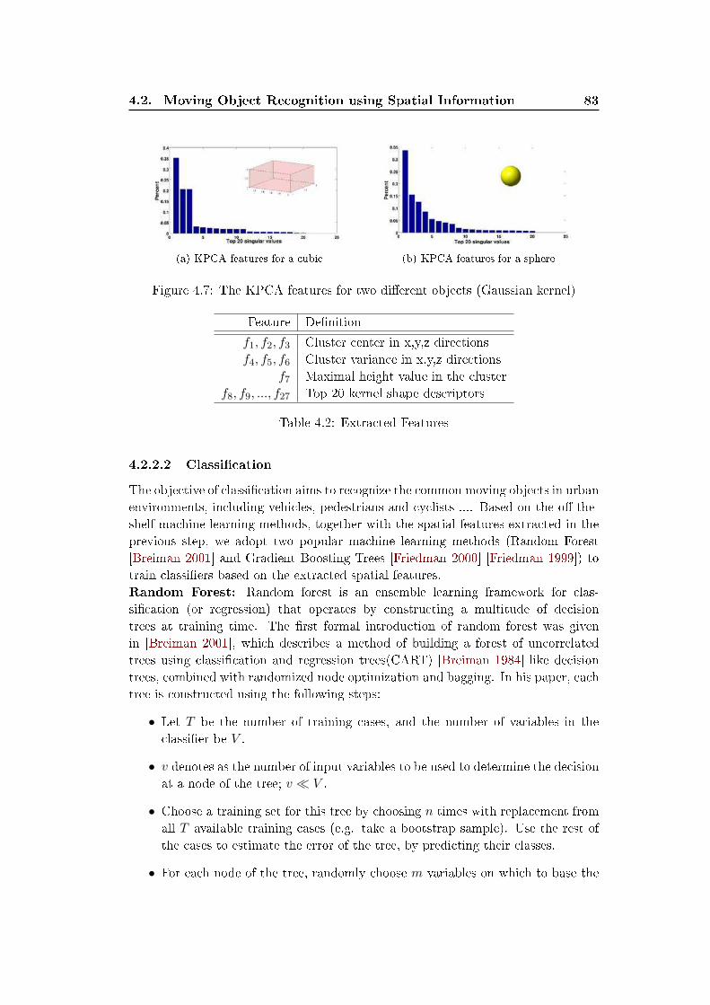
4.2. Moving Object Recognition using Spatial Information 83
(a) KPCA features for a cubic (b) KPCA features for a sphere
Figure 4.7: The KPCA features for two di�erent objects (Gaussian kernel)
Feature De�nition
f1, f2, f3 Cluster center in x,y,z directions
f4, f5, f6 Cluster variance in x,y,z directions
f7 Maximal height value in the cluster
f8, f9, ..., f27 Top 20 kernel shape descriptors
Table 4.2: Extracted Features
4.2.2.2 Classi�cation
The objective of classi�cation aims to recognize the common moving objects in urban
environments, including vehicles, pedestrians and cyclists .... Based on the o�-the-
shelf machine learning methods, together with the spatial features extracted in the
previous step, we adopt two popular machine learning methods (Random Forest
[Breiman 2001] and Gradient Boosting Trees [Friedman 2000] [Friedman 1999]) to
train classi�ers based on the extracted spatial features.
Random Forest: Random forest is an ensemble learning framework for clas-
si�cation (or regression) that operates by constructing a multitude of decision
trees at training time. The �rst formal introduction of random forest was given
in [Breiman 2001], which describes a method of building a forest of uncorrelated
trees using classi�cation and regression trees(CART) [Breiman 1984] like decision
trees, combined with randomized node optimization and bagging. In his paper, each
tree is constructed using the following steps:
• Let T be the number of training cases, and the number of variables in the
classi�er be V .
• v denotes as the number of input variables to be used to determine the decision
at a node of the tree; v ≪ V .
• Choose a training set for this tree by choosing n times with replacement from
all T available training cases (e.g. take a bootstrap sample). Use the rest of
the cases to estimate the error of the tree, by predicting their classes.
• For each node of the tree, randomly choose m variables on which to base the
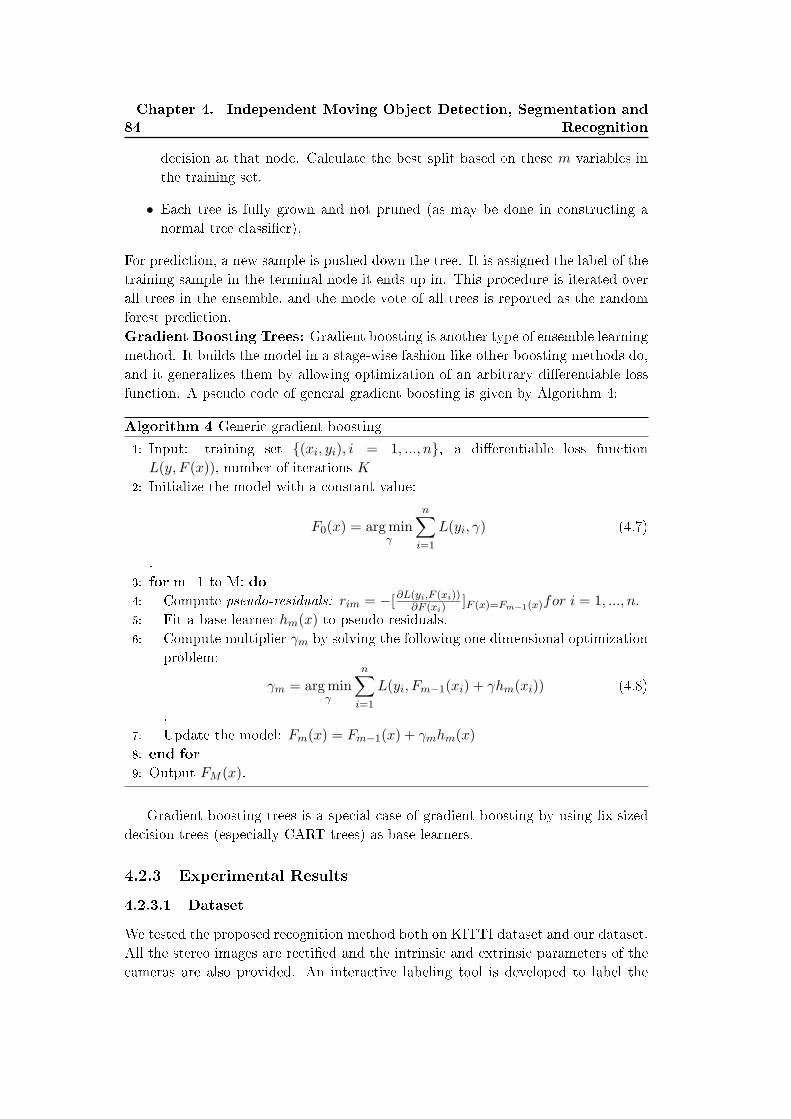
84Chapter 4. Independent Moving Object Detection, Segmentation and
Recognition
decision at that node. Calculate the best split based on these m variables in
the training set.
• Each tree is fully grown and not pruned (as may be done in constructing a
normal tree classi�er).
For prediction, a new sample is pushed down the tree. It is assigned the label of the
training sample in the terminal node it ends up in. This procedure is iterated over
all trees in the ensemble, and the mode vote of all trees is reported as the random
forest prediction.
Gradient Boosting Trees: Gradient boosting is another type of ensemble learningmethod. It builds the model in a stage-wise fashion like other boosting methods do,
and it generalizes them by allowing optimization of an arbitrary di�erentiable loss
function. A pseudo code of general gradient boosting is given by Algorithm 4:
Algorithm 4 Generic gradient boosting
1: Input: training set {(xi, yi), i = 1, ..., n}, a di�erentiable loss function
L(y, F (x)), number of iterations K
2: Initialize the model with a constant value:
F0(x) = argminγ
n∑
i=1
L(yi, γ) (4.7)
.
3: for m=1 to M: do4: Compute pseudo-residuals: rim = −[∂L(yi,F (xi))
∂F (xi)]F (x)=Fm−1(x)for i = 1, ..., n.
5: Fit a base learner hm(x) to pseudo-residuals.
6: Compute multiplier γm by solving the following one dimensional optimization
problem:
γm = argminγ
n∑
i=1
L(yi, Fm−1(xi) + γhm(xi)) (4.8)
.
7: Update the model: Fm(x) = Fm−1(x) + γmhm(x)
8: end for9: Output FM (x).
Gradient boosting trees is a special case of gradient boosting by using �x-sized
decision trees (especially CART trees) as base learners.
4.2.3 Experimental Results
4.2.3.1 Dataset
We tested the proposed recognition method both on KITTI dataset and our dataset.
All the stereo images are recti�ed and the intrinsic and extrinsic parameters of the
cameras are also provided. An interactive labeling tool is developed to label the
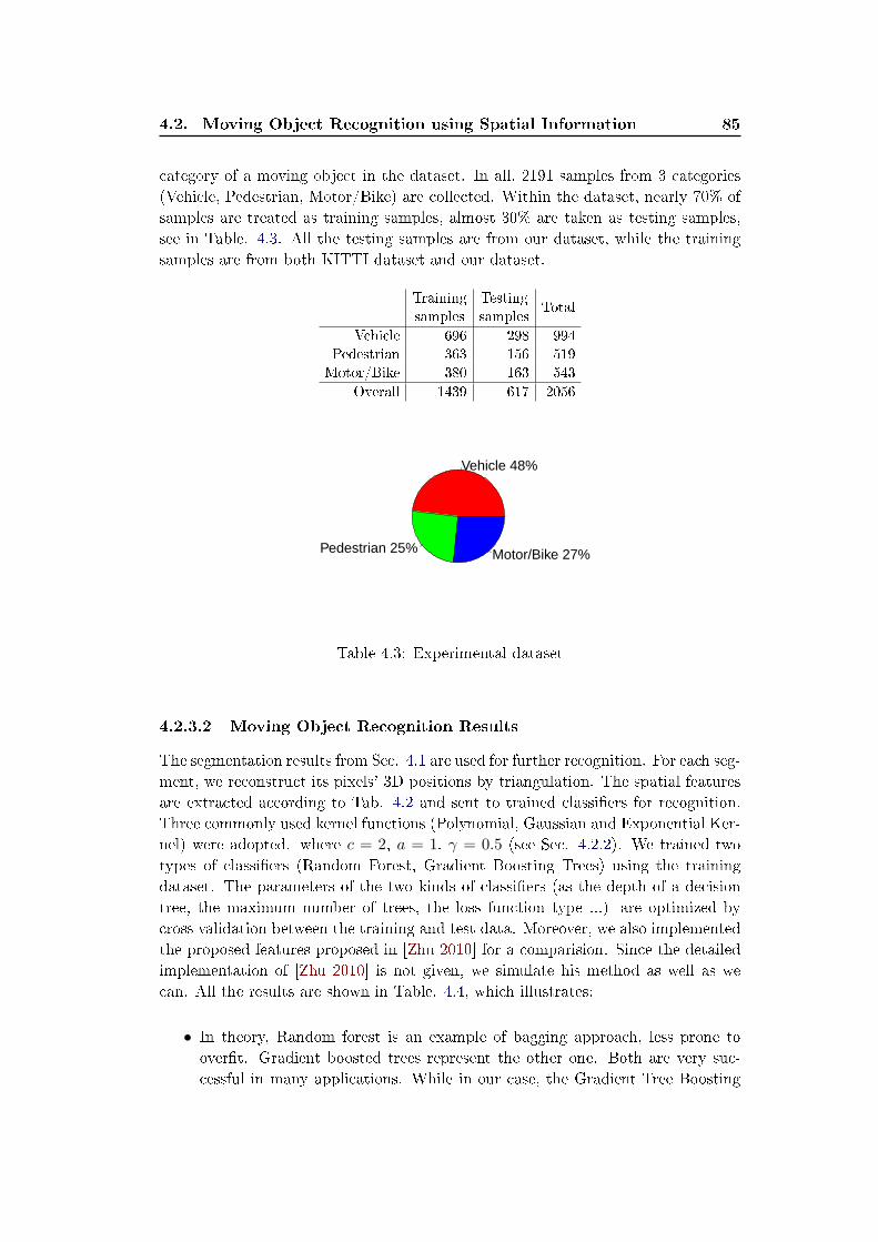
4.2. Moving Object Recognition using Spatial Information 85
category of a moving object in the dataset. In all, 2191 samples from 3 categories
(Vehicle, Pedestrian, Motor/Bike) are collected. Within the dataset, nearly 70% of
samples are treated as training samples, almost 30% are taken as testing samples,
see in Table. 4.3. All the testing samples are from our dataset, while the training
samples are from both KITTI dataset and our dataset.
Training
samples
Testing
samplesTotal
Vehicle 696 298 994
Pedestrian 363 156 519
Motor/Bike 380 163 543
Overall 1439 617 2056
Vehicle 48%
Pedestrian 25% Motor/Bike 27%
Table 4.3: Experimental dataset
4.2.3.2 Moving Object Recognition Results
The segmentation results from Sec. 4.1 are used for further recognition. For each seg-
ment, we reconstruct its pixels' 3D positions by triangulation. The spatial features
are extracted according to Tab. 4.2 and sent to trained classi�ers for recognition.
Three commonly used kernel functions (Polynomial, Gaussian and Exponential Ker-
nel) were adopted. where c = 2, a = 1, γ = 0.5 (see Sec. 4.2.2). We trained two
types of classi�ers (Random Forest, Gradient Boosting Trees) using the training
dataset. The parameters of the two kinds of classi�ers (as the depth of a decision
tree, the maximum number of trees, the loss function type ...) are optimized by
cross validation between the training and test data. Moreover, we also implemented
the proposed features proposed in [Zhu 2010] for a comparision. Since the detailed
implementation of [Zhu 2010] is not given, we simulate his method as well as we
can. All the results are shown in Table. 4.4, which illustrates:
• In theory, Random forest is an example of bagging approach, less prone to
over�t. Gradient boosted trees represent the other one. Both are very suc-
cessful in many applications. While in our case, the Gradient Tree Boosting

86Chapter 4. Independent Moving Object Detection, Segmentation and
Recognition
classi�er performs better than Random Forest classi�er in all the cases in our
dataset.
• The classi�cation results based on the three kinds of kernels are almost the
same. However, the Gaussian kernel performs slightly better than the other
two kernels.
• Compared with Zhu's method [Zhu 2010], the proposed kernel shape descrip-
tors improve the classi�cation results thanks to transforming the features into
a higher dimensional space. In average, the precision based on the proposed
kernel shape descriptors increases by around 10% than in [Zhu 2010].
• The Confusion matrices reveal that pedestrians and cyclists samples are apt
to be confused. This is because they are similar in both size and shape.
The experimental results for the moving object recognition are shown in Fig.
4.8.
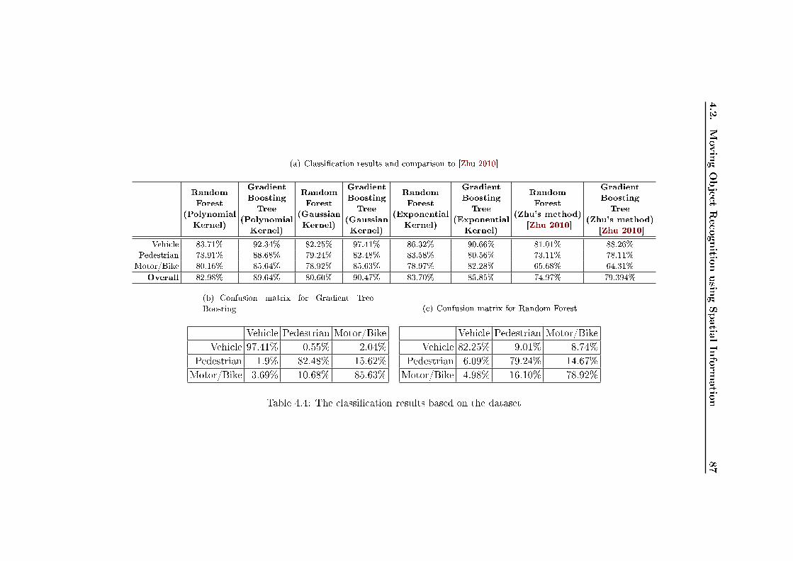
4.2.
Mov
ingObject
Reco
gnitio
nusin
gSpatial
Inform
ation
87
(a) Classi�cation results and comparison to [Zhu 2010]
Random
Forest
(Polynomial
Kernel)
Gradient
Boosting
Tree
(Polynomial
Kernel)
Random
Forest
(Gaussian
Kernel)
Gradient
Boosting
Tree
(Gaussian
Kernel)
Random
Forest
(Exponential
Kernel)
Gradient
Boosting
Tree
(Exponential
Kernel)
Random
Forest
(Zhu's method)
[Zhu 2010]
Gradient
Boosting
Tree
(Zhu's method)
[Zhu 2010]
Vehicle 83.71% 92.34% 82.25% 97.41% 86.32% 90.66% 81.01% 88.26%
Pedestrian 78.91% 88.68% 79.24% 82.48% 83.58% 80.56% 73.11% 78.11%
Motor/Bike 80.16% 85.64% 78.92% 85.63% 78.97% 82.28% 65.68% 64.31%
Overall 82.98% 89.64% 80.60% 90.47% 83.70% 85.85% 74.97% 79.394%
(b) Confusion matrix for Gradient Tree
Boosting
Vehicle Pedestrian Motor/Bike
Vehicle 97.41% 0.55% 2.04%
Pedestrian 1.9% 82.48% 15.62%
Motor/Bike 3.69% 10.68% 85.63%
(c) Confusion matrix for Random Forest
Vehicle Pedestrian Motor/Bike
Vehicle 82.25% 9.01% 8.74%
Pedestrian 6.09% 79.24% 14.67%
Motor/Bike 4.98% 16.10% 78.92%
Table 4.4: The classi�cation results based on the dataset
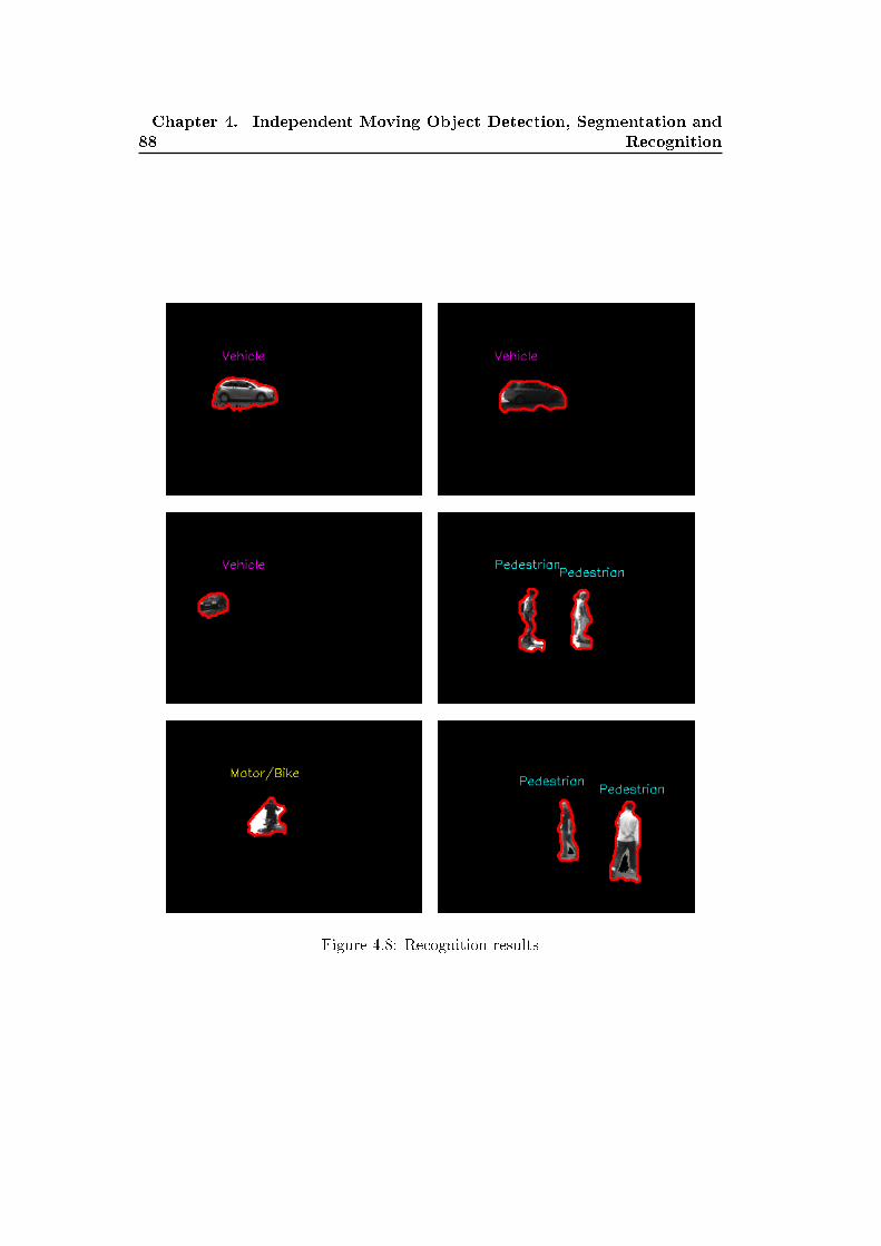
88Chapter 4. Independent Moving Object Detection, Segmentation and
Recognition
Figure 4.8: Recognition results
4.3. Conclusion and Future Works 89
4.3 Conclusion and Future Works
In this chapter, we proposed stereo vision based methods to detect, segment and rec-
ognize independent moving objects, for a moving intelligent vehicle. These methods
are based on the ego-motion estimation results in Chap. 3.
In the �rst part, we presented a stereo vision based method to detect and seg-
ment independent moving objects from a moving intelligent vehicle. The method
relies on the "outliers" generated in the step of visual odometry. The "outliers"
mainly consist of matching noises and feature points from moving objects. Next,
they are projected to U-disparity image as seeds for moving object detection and
segmentation. This method is tested on our datasets and the experimental results
are analyzed. However, the performance of this method degenerates when trying to
detect moving pedestrians. The main reason of this problem is that moving pedestri-
ans usually move too slow to e�ectively detect their motion between two consecutive
frames. Future works would be around this problem. One possible solution to this
problem is using pedestrian detection methods detect pedestrians at �rst. Then, if
there are any detected moving feature points in detected pedestrian region, it could
be classi�ed as a moving pedestrian.
In the second part, a recognition approach based on learning spatial informa-
tion is proposed. We tried to classify the segmented moving objects acquired by
the previous step. In this method, a kernel PCA algorithm is used to select the
spatial features in high dimensional space. Next, we trained two kinds of classi�ers:
Random Forest and Gradient Boosting Trees to recognize three kinds of moving ob-
jects: Pedestrian, Vehicle and Motor/Bike. The experimental results showed good
recognition rates, especially for the Gaussian kernel based KPCA features combin-
ing with Gradient Boosting Trees. Also, we show that with the boosted kernel PCA
features, our method outperforms an another method by around 10% in terms of
precision. In future works, we consider combining spatial features with appearance
features to reach a better recognition results. For example, the histogram of oriented
gradients (HoG) or local binary patterns (LBP) could be introduced to improve the
recognition performance.

Chapter 5
Extrinsic Calibration between a
Stereo Vision System and a Lidar
Contents
5.1 Introduction . . . . . . . . . . . . . . . . . . . . . . . . . . . . 91
5.1.1 Related works . . . . . . . . . . . . . . . . . . . . . . . . . . . 92
5.1.2 Problem Formulation . . . . . . . . . . . . . . . . . . . . . . 93
5.1.3 Performance Evaluation . . . . . . . . . . . . . . . . . . . . . 94
5.2 3D Plane Reconstruction based Extrinsic Calibration . . . 95
5.2.1 Corner Points Triangulation . . . . . . . . . . . . . . . . . . . 96
5.2.2 3D Plane Estimation . . . . . . . . . . . . . . . . . . . . . . . 96
5.2.3 Automatic Lidar Measurements Extraction . . . . . . . . . . 100
5.2.4 Estimating Rigid Transformation between the lidar and the
Stereoscopic System . . . . . . . . . . . . . . . . . . . . . . . 101
5.2.5 Summary of the Calibration Procedure . . . . . . . . . . . . . 103
5.3 Experimental Results . . . . . . . . . . . . . . . . . . . . . . . 104
5.3.1 Computer Simulations . . . . . . . . . . . . . . . . . . . . . . 104
5.3.2 Real Data Test . . . . . . . . . . . . . . . . . . . . . . . . . . 110
5.3.3 Outdoor Experiments . . . . . . . . . . . . . . . . . . . . . . 111
5.4 Conclusion And Future Work . . . . . . . . . . . . . . . . . . 116
The previous chapters focus in solving several perception missions only by stereo
vision sytem. A real intelligent vehicle, as introduced in Sec. 1, usually equips with
multiple sensors. In this thesis, we also use a 2D lidar to perform the perception
tasks. In order to fuse the two kinds of sensor measurement, an extrinsic calibration
method aimed to estimate a 3D rigid transformation between the two sensors is
proposed and performed.
5.1 Introduction
As we introduced in the �rst chapter, we plan to use stereoscopic system and 2D
lidar to analyze the environment for an intelligent vehicle. However, despite many
impressive progresses in both computer vision, and range sensors in past decades, no
technique based on single kind of sensors can be reliably and robustly performed in
92Chapter 5. Extrinsic Calibration between a Stereo Vision System and
a Lidar
real complex environments. In fact, visual sensors are always limited in narrow �eld
of views (FOV) and require huge computational cost. On the other hand, providing
only depth information, the range sensors are not enough for more complex tasks
in deep level. Hence, achieving e�ective and robust environments understanding
requires the fusion of di�erent kinds of sensors. Indeed, fusing visual and range data
has attracted more and more attentions for intelligent vehicles. In [Mahlisch 2006,
Fox 2007,Hwang 2007], various information fusion methods are proposed.
The problem of fusing data between visual cameras and LIDARs arises from the
heterogeneity of the sensors. Lidar data is depth information in a certain scan plan,
while the data of a camera can be viewed as a projection of a 3D world into an
image plane. Thus, how to bridge the gap between a visual camera and a LIDAR
has to be solved before performing data fusion. An initial solution is to estimate
a rigid geometrical transformation (a 3× 3 rotation matrix and a 3× 1 translation
vector) between lidar coordinate system and stereo vision coordinate system � which
is usually called extrinsic calibration between lidar and stereo vision system. In
general, it is implemented as the �rst step for further information integration of the
two sensors, as illustrated in [Perrollaz 2006,Cristiano 2009,Huang 2009b].
5.1.1 Related works
In literature, most proposed methods for extrinsic calibration between a lidar and
a camera can be roughly divided into three categories:
1. Methods based on auxiliary sensors. In [Aliakbarpour 2009], with the aid of
an IMU (Inertial Measurement Unit) and a visible laser point, the Euclidean
3-dimensional transformation between a lidar and a camera is acquired by
rotating the scan plane, where the angular information is estimated by the
inertial sensor. Nunez et al. [Nunez 2009] also use an IMU to construct ge-
ometric constraints between a lidar and a camera system for calculating the
transformation. However, being equipped with an IMU is a prerequisite for
this kind of approaches.
2. Methods based on specially designed calibration boards. Li et al. [Li 2007] design
a right-angled triangular checkerboard and employ the invisible intersection
points of the lidar's scan plane with the edges of the checkerboard to set up
constraint equations. Rodriguez et al. [Rodriguez F 2008] adopt a calibration
board with two concentric circles where the inner circle is hollowed. The au-
thors use the correspondence of the center of the inner circle between several
di�erent poses to achieve extrinsic calibration. By making use of special fea-
tures in the designed calibration board, such approaches enable one to acquire
the geometric relationship between a lidar and a camera. However, specially
designed calibration boards impede themself for more widespread uses.
3. Methods based on common calibration chessboards. Zhang and Pless
[Zhang 2004] �rstly proposed a method utilizing an ordinary calibration chess-
board which is widely used in camera calibration. This method is based on
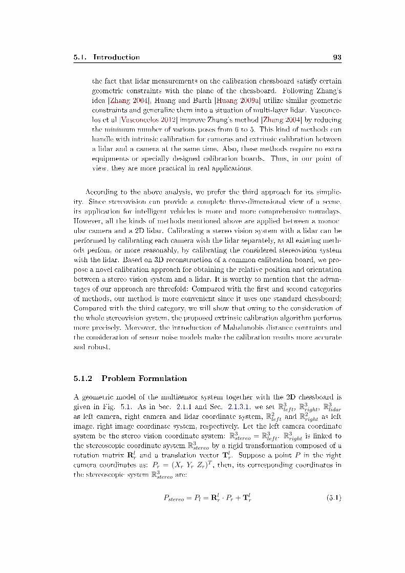
5.1. Introduction 93
the fact that lidar measurements on the calibration chessboard satisfy certain
geometric constraints with the plane of the chessboard. Following Zhang's
idea [Zhang 2004], Huang and Barth [Huang 2009a] utilize similar geometric
constraints and generalize them into a situation of multi-layer lidar. Vasconce-
los et al [Vasconcelos 2012] improve Zhang's method [Zhang 2004] by reducing
the minimum number of various poses from 6 to 5. This kind of methods can
handle with intrinsic calibration for cameras and extrinsic calibration between
a lidar and a camera at the same time. Also, these methods require no extra
equipments or specially designed calibration boards. Thus, in our point of
view, they are more practical in real applications.
According to the above analysis, we prefer the third approach for its simplic-
ity. Since stereovision can provide a complete three-dimensional view of a scene,
its application for intelligent vehicles is more and more comprehensive nowadays.
However, all the kinds of methods mentioned above are applied between a monoc-
ular camera and a 2D lidar. Calibrating a stereo vision system with a lidar can be
performed by calibrating each camera with the lidar separately, as all existing meth-
ods perfom, or more reasonably, by calibrating the considered stereovision system
with the lidar. Based on 3D reconstruction of a common calibration board, we pro-
pose a novel calibration approach for obtaining the relative position and orientation
between a stereo vision system and a lidar. It is worthy to mention that the advan-
tages of our approach are threefold: Compared with the �rst and second categories
of methods, our method is more convenient since it uses one standard chessboard;
Compared with the third category, we will show that owing to the consideration of
the whole stereovision system, the proposed extrinsic calibration algorithm performs
more precisely. Moreover, the introduction of Mahalanobis distance contraints and
the consideration of sensor noise models make the calibration results more accurate
and robust.
5.1.2 Problem Formulation
A geometric model of the multisensor system together with the 2D chessboard is
given in Fig. 5.1. As in Sec. 2.1.1 and Sec. 2.1.3.1, we set R3left, R
3right, R
3lidar
as left camera, right camera and lidar coordinate system, R2left and R
2right as left
image, right image coordinate system, respectively. Let the left camera coordinate
system be the stereo vision coordinate system: R3stereo = R
3left. R
3right is linked to
the stereoscopic coordinate system R3stereo by a rigid transformation composed of a
rotation matrix Rlr and a translation vector Tl
r. Suppose a point P in the right
camera coordinates as: Pr = (Xr Yr Zr)T , then, its corresponding coordinates in
the stereoscopic system R3stereo are:
Pstereo = Pl = Rlr · Pr +Tl
r (5.1)
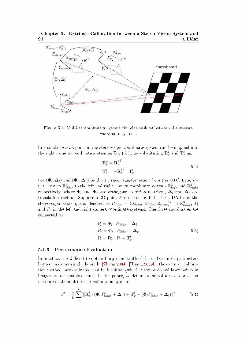
94Chapter 5. Extrinsic Calibration between a Stereo Vision System and
a Lidar
Figure 5.1: Multi-sensor system: geometric relationships between the sensors
coordinate systems
In a similar way, a point in the stereoscopic coordinate system can be mapped into
the right camera coordinate system as Eq. (5.1), by substituting Rlr and Tl
r as:
Rrl = Rl
rT
Trl = −Rl
rT ·Tl
r
(5.2)
Let (Φl,∆l) and (Φr,∆r) be the 3D rigid transformation from the LIDAR coordi-
nate system R3lidar to the left and right camera coordinate systems R3
left and R3right
respectively, where Φl and Φr are orthogonal rotation matrixes, ∆l and ∆r are
translation vectors. Suppose a 3D point P observed by both the LIDAR and the
stereoscopic system, and denoted as Plidar = (Xlidar Ylidar Zlidar)T in R
3lidar, Pl
and Pr in the left and right camera coordinate systems. The three coordinates are
connected by:
Pl = Φl · Plidar +∆l
Pr = Φr · Plidar +∆r
Pl = Rlr · Pr +Tl
r
(5.3)
5.1.3 Performance Evaluation
In practice, it is di�cult to obtain the ground truth of the real extrinsic parameters
between a camera and a lidar. In [Zhang 2004], [Huang 2009b], the extrinsic calibra-
tion methods are evaluated just by intuition (whether the projected laser points in
images are reasonable or not). In this paper, we de�ne an indicator ε as a precision
measure of the multi-sensor calibration system:
ε2 =1
L
L∑
i
∥Rlr · (ΦrP
ilidar +∆r) +Tl
r − (ΦlPilidar +∆l)∥2 (5.4)
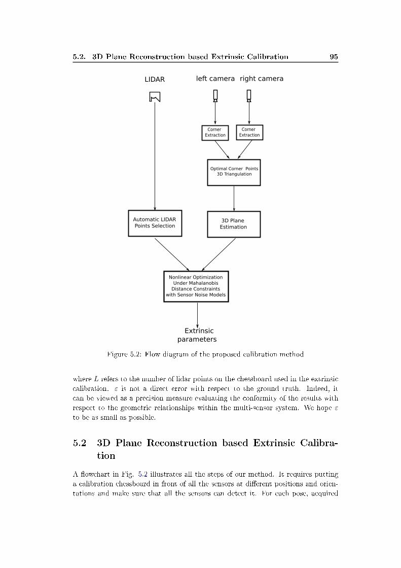
5.2. 3D Plane Reconstruction based Extrinsic Calibration 95
Corner
Extraction
Corner
Extraction
Optimal Corner Points
3D Triangulation
3D Plane
Estimation
Nonlinear Optimization
Under Mahalanobis
Distance Constraints
with Sensor Noise Models
Automatic LIDAR
Points Selection
LIDAR left camera right camera
Extrinsic
parameters
Figure 5.2: Flow diagram of the proposed calibration method
where L refers to the number of lidar points on the chessboard used in the extrinsic
calibration. ε is not a direct error with respect to the ground truth. Indeed, it
can be viewed as a precision measure evaluating the conformity of the results with
respect to the geometric relationships within the multi-sensor system. We hope ε
to be as small as possible.
5.2 3D Plane Reconstruction based Extrinsic Calibra-
tion
A �owchart in Fig. 5.2 illustrates all the steps of our method. It requires putting
a calibration chessboard in front of all the sensors at di�erent positions and orien-
tations and make sure that all the sensors can detect it. For each pose, acquired
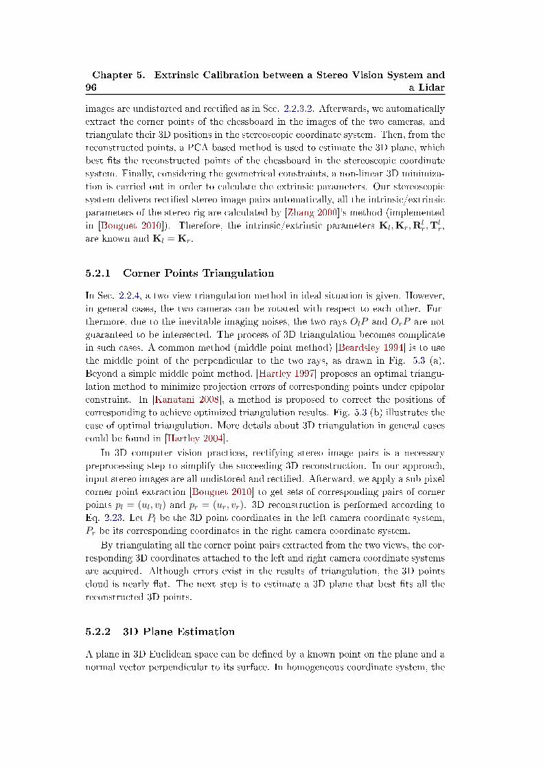
96Chapter 5. Extrinsic Calibration between a Stereo Vision System and
a Lidar
images are undistorted and recti�ed as in Sec. 2.2.3.2. Afterwards, we automatically
extract the corner points of the chessboard in the images of the two cameras, and
triangulate their 3D positions in the stereoscopic coordinate system. Then, from the
reconstructed points, a PCA based method is used to estimate the 3D plane, which
best �ts the reconstructed points of the chessboard in the stereoscopic coordinate
system. Finally, considering the geometrical constraints, a non-linear 3D minimiza-
tion is carried out in order to calculate the extrinsic parameters. Our stereoscopic
system delivers recti�ed stereo image pairs automatically, all the intrinsic/extrinsic
parameters of the stereo-rig are calculated by [Zhang 2000]'s method (implemented
in [Bouguet 2010]). Therefore, the intrinsic/extrinsic parameters Kl,Kr,Rlr,T
lr,
are known and Kl = Kr.
5.2.1 Corner Points Triangulation
In Sec. 2.2.4, a two-view triangulation method in ideal situation is given. However,
in general cases, the two cameras can be rotated with respect to each other. Fur-
thermore, due to the inevitable imaging noises, the two rays OlP and OrP are not
guaranteed to be intersected. The process of 3D triangulation becomes complicate
in such cases. A common method (middle point method) [Beardsley 1994] is to use
the middle point of the perpendicular to the two rays, as drawn in Fig. 5.3 (a).
Beyond a simple middle point method, [Hartley 1997] proposes an optimal triangu-
lation method to minimize projection errors of corresponding points under epipolar
constraint. In [Kanatani 2008], a method is proposed to correct the positions of
corresponding to achieve optimized triangulation results. Fig. 5.3 (b) illustrates the
case of optimal triangulation. More details about 3D triangulation in general cases
could be found in [Hartley 2004].
In 3D computer vision practices, rectifying stereo image pairs is a necessary
preprocessing step to simplify the succeeding 3D reconstruction. In our approach,
input stereo images are all undistored and recti�ed. Afterward, we apply a sub-pixel
corner point extraction [Bouguet 2010] to get sets of corresponding pairs of corner
points pl = (ul, vl) and pr = (ur, vr). 3D reconstruction is performed according to
Eq. 2.23. Let Pl be the 3D point coordinates in the left camera coordinate system,
Pr be its corresponding coordinates in the right camera coordinate system.
By triangulating all the corner point pairs extracted from the two views, the cor-
responding 3D coordinates attached to the left and right camera coordinate systems
are acquired. Although errors exist in the results of triangulation, the 3D points
cloud is nearly �at. The next step is to estimate a 3D plane that best �ts all the
reconstructed 3D points.
5.2.2 3D Plane Estimation
A plane in 3D Euclidean space can be de�ned by a known point on the plane and a
normal vector perpendicular to its surface. In homogeneous coordinate system, the
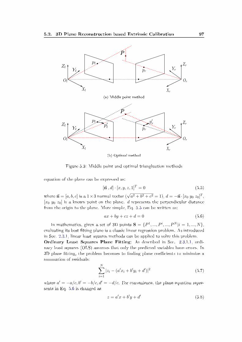
5.2. 3D Plane Reconstruction based Extrinsic Calibration 97
(a) Middle point method
(b) Optimal method
Figure 5.3: Middle point and optimal triangluation methods
equation of the plane can be expressed as:
[n , d] · [x, y, z, 1]T = 0 (5.5)
where n = [a, b, c] is a 1×3 normal vector (√a2 + b2 + c2 = 1), d = −n · [x0 y0 z0]T ,
[x0 y0 z0] is a known point on the plane. d represents the perpendicular distance
from the origin to the plane. More simple, Eq. 5.5 can be written as:
ax+ by + cz + d = 0 (5.6)
In mathematics, given a set of 3D points S = {P 1, ..., P i, ..., PN |i = 1, ..., N},evaluating its best �tting plane is a classic linear regression problem. As introduced
in Sec. 2.3.1, linear least squares methods can be applied to solve this problem.
Ordinary Least Squares Plane Fitting: As described in Sec. 2.3.1.1, ordi-
nary least squares (OLS) assumes that only the predicted variables have errors. In
3D plane �tting, the problem becomes to �nding plane coe�cients to minimize a
summation of residuals:
N∑
i=1
|zi − (a′xi + b′yi + d′)|2 (5.7)
where a′ = −a/c, b′ = −b/c, d′ = −d/c. For convenience, the plane equation repre-
sents in Eq. 5.6 is changed as
z = a′x+ b′y + d′ (5.8)
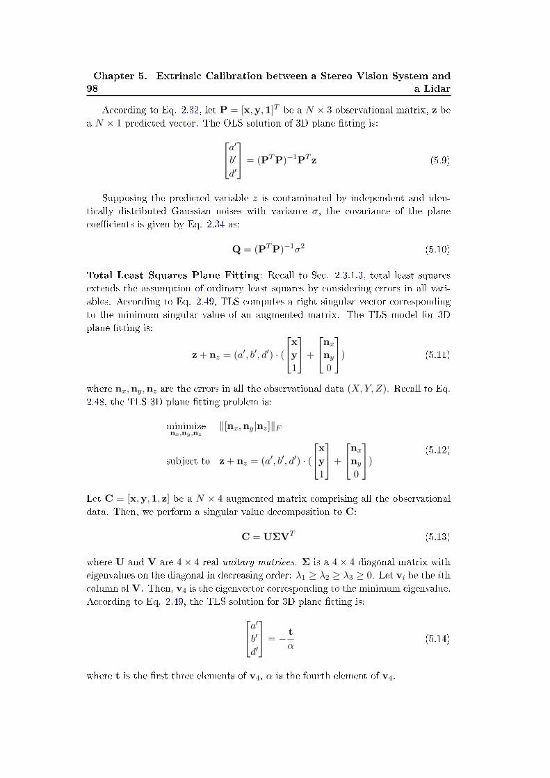
98Chapter 5. Extrinsic Calibration between a Stereo Vision System and
a Lidar
According to Eq. 2.32, let P = [x,y,1]T be a N × 3 observational matrix, z be
a N × 1 predicted vector. The OLS solution of 3D plane �tting is:
a′
b′
d′
= (PTP)−1PT z (5.9)
Supposing the predicted variable z is contaminated by independent and iden-
tically distributed Gaussian noises with variance σ, the covariance of the plane
coe�cients is given by Eq. 2.34 as:
Q = (PTP)−1σ2 (5.10)
Total Least Squares Plane Fitting: Recall to Sec. 2.3.1.3, total least squares
extends the assumption of ordinary least squares by considering errors in all vari-
ables. According to Eq. 2.49, TLS computes a right singular vector corresponding
to the minimum singular value of an augmented matrix. The TLS model for 3D
plane �tting is:
z+ nz = (a′, b′, d′) · (
x
y
1
+
nx
ny
0
) (5.11)
where nx,ny,nz are the errors in all the observational data (X,Y, Z). Recall to Eq.
2.48, the TLS 3D plane �tting problem is:
minimizenx,ny ,nz
∥[nx,ny|nz]∥F
subject to z+ nz = (a′, b′, d′) · (
x
y
1
+
nx
ny
0
)(5.12)
Let C = [x,y,1, z] be a N × 4 augmented matrix comprising all the observational
data. Then, we perform a singular value decomposition to C:
C = UΣVT (5.13)
where U and V are 4× 4 real unitary matrices. Σ is a 4× 4 diagonal matrix with
eigenvalues on the diagonal in decreasing order: λ1 ≥ λ2 ≥ λ3 ≥ 0. Let vi be the ith
column of V. Then, v4 is the eigenvector corresponding to the minimum eigenvalue.
According to Eq. 2.49, the TLS solution for 3D plane �tting is:
a′
b′
d′
= − t
α(5.14)
where t is the �rst three elements of v4, α is the fourth element of v4.
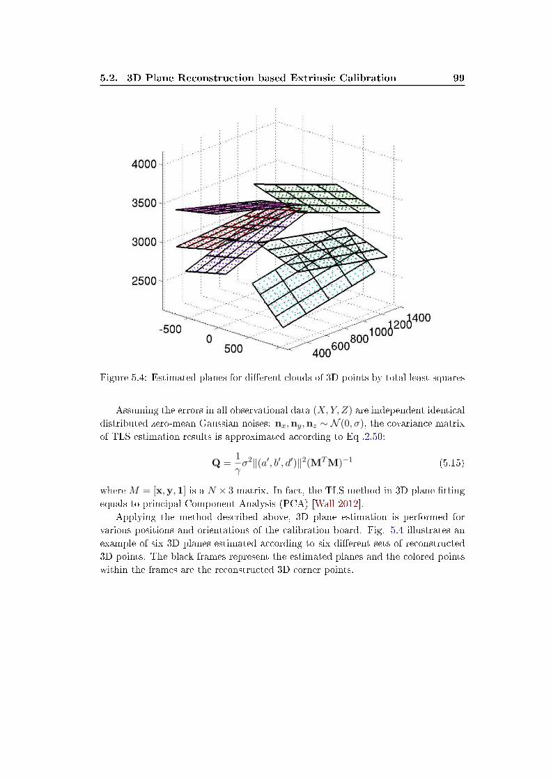
5.2. 3D Plane Reconstruction based Extrinsic Calibration 99
Figure 5.4: Estimated planes for di�erent clouds of 3D points by total least squares
Assuming the errors in all observational data (X,Y, Z) are independent identical
distributed zero-mean Gaussian noises: nx,ny,nz ∼ N (0, σ), the covariance matrix
of TLS estimation results is approximated according to Eq .2.50:
Q =1
γσ2∥(a′, b′, d′)∥2(MTM)−1 (5.15)
where M = [x,y,1] is a N × 3 matrix. In fact, the TLS method in 3D plane �tting
equals to principal Component Analysis (PCA) [Wall 2012].
Applying the method described above, 3D plane estimation is performed for
various positions and orientations of the calibration board. Fig. 5.4 illustrates an
example of six 3D planes estimated according to six di�erent sets of reconstructed
3D points. The black frames represent the estimated planes and the colored points
within the frames are the reconstructed 3D corner points.
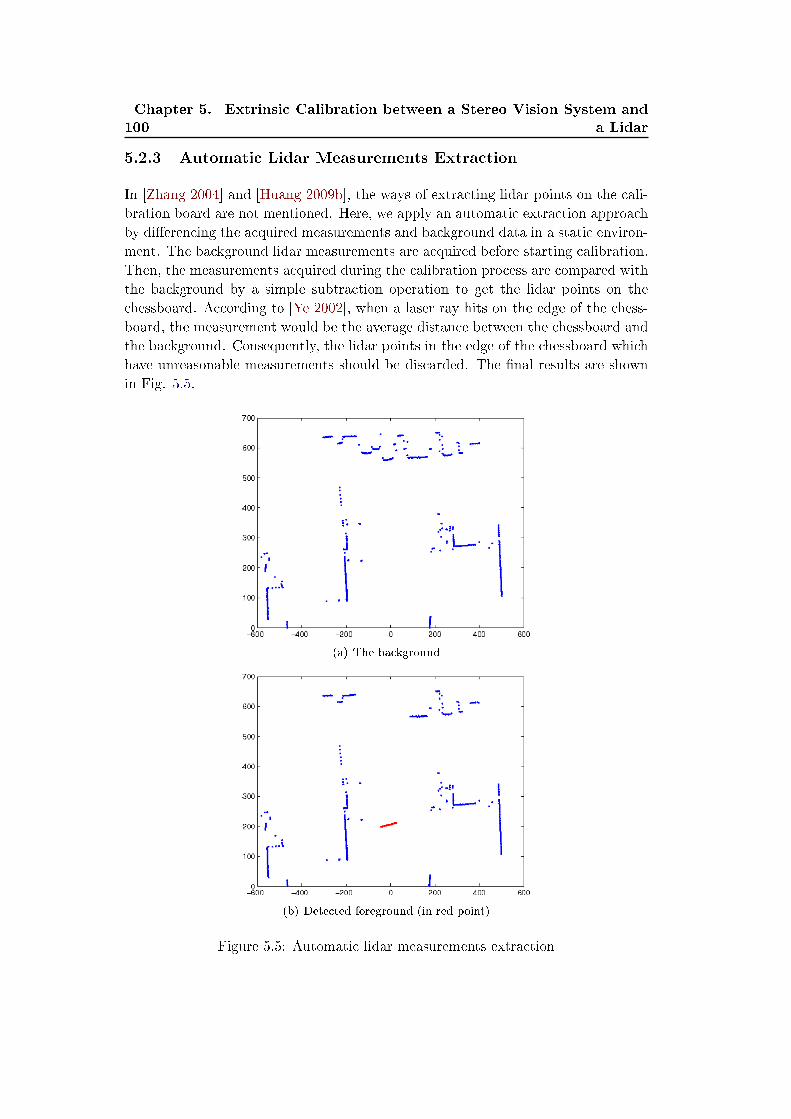
100Chapter 5. Extrinsic Calibration between a Stereo Vision System and
a Lidar
5.2.3 Automatic Lidar Measurements Extraction
In [Zhang 2004] and [Huang 2009b], the ways of extracting lidar points on the cali-
bration board are not mentioned. Here, we apply an automatic extraction approach
by di�erencing the acquired measurements and background data in a static environ-
ment. The background lidar measurements are acquired before starting calibration.
Then, the measurements acquired during the calibration process are compared with
the background by a simple subtraction operation to get the lidar points on the
chessboard. According to [Ye 2002], when a laser ray hits on the edge of the chess-
board, the measurement would be the average distance between the chessboard and
the background. Consequently, the lidar points in the edge of the chessboard which
have unreasonable measurements should be discarded. The �nal results are shown
in Fig. 5.5.
(a) The background
(b) Detected foreground (in red point)
Figure 5.5: Automatic lidar measurements extraction
5.2. 3D Plane Reconstruction based Extrinsic Calibration 101
5.2.4 Estimating Rigid Transformation between the lidar and the
Stereoscopic System
The steps presented above allow us to estimate 3D planes of the calibration board
with various poses (j = 1, ...,M). In ideal situations, every lidar measurement on
the calibration board should satisfy the plane equation of the calibration board:
N · Pstereo = N ·H · Plidar = 0 (5.16)
where H =
[
Φl ∆l
0 1
]
denotes 3D rigid transformation which we want to estimate.
N = [n, d] = [a, b, c, d] is the estimated 3D plane of the chessboard.
However, in real experiments, Eq. 5.16 is rarely satis�ed. Given an estimated
rigid transformation H, all the residuals can be represented as:
e = {N1HP 1,1lidar . . . N1HPL1,1
lidar . . . NMHP 1,Mlidar . . . NMHPLM ,M
lidar } (5.17)
where P k,jlidar|(k = 1, ..., Lj , j = 1, ...M) is the homogeneous coordinate of the kth
lidar point on the chessboard at the jth pose. Nj |(j = 1, ...M) is the 3D plane of
the chessboard put at the jth pose.
Although directly minimizing a summation of squared errors in Eq.(5.17) makes
sense, it doesn't take into account enough the errors produced either from the 3D
plane equations estimated by the stereovision system or from the lidar itself. Con-
sidering the error of 3D triangulation grows quadratically, this could make results
worse when the calibration board is far away from the stereovision system. To make
the method more robust against errors, we propose to minimize a summation of
squared Mahalanobis distance, rather than Euclidean distance. Compared with Eu-
clidean metric, the Mahalanobis distance bene�ts can be viewed as follows: �rstly,
it corrects the scale factor. In our work, the errors come from both stereoscopic
system and lidar. Euclidean distance is sensitive to the scale of various kinds of
variables involved. For Mahalanobis distance, thanks to the measure of covariance,
the problem of scale factor is resolved. Secondly, Mahalanobis distance corrects the
correlation between variables. This advantage is also a consequence of calculating
covariance. Assuming e ∽ N (0, C), then the optimization of extrinsic parameters
based on Mahalanobis distance becomes:
H(Φl,∆l) = argminΦl,∆l
{eTC−1e} (5.18)
where C is the covariance matrix of e. Assuming the elements of e in Eq.(5.17) are
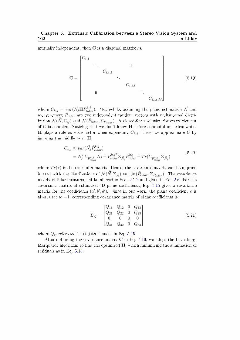
102Chapter 5. Extrinsic Calibration between a Stereo Vision System and
a Lidar
mutually independent, then C is a diagonal matrix as:
C =
C1,1
. . . 0
CL1,1
. . .
C1,M
0. . .
CLM ,M
(5.19)
where Ck,j = var(NjHP k,jlidar). Meanwhile, assuming the plane estimation N and
measurement Plidar are two independent random vectors with multinormal distri-
bution N (¯N,ΣN ) and N (Plidar,ΣPlidar
). A closed-form solution for every element
of C is complex. Noticing that we don't know H before computation. Meanwhile,
H plays a role as scale factor when expanding Ck,j . Here, we approximate C by
ignoring the middle term H:
Ck,j ≈ var(NjPk,jlidar)
=¯NT
j ΣPk,jlidar
¯Nj + P k,jT
lidarΣNjP k,jlidar + Tr(Σ
Pk,jlidar
ΣNj)
(5.20)
where Tr(∗) is the trace of a matrix. Hence, the covariance matrix can be approx-
imated with the distributions of N (¯N,ΣN ) and N (Plidar,ΣPlidar
). The covariance
matrix of lidar measurement is inferred in Sec. 2.1.2 and given in Eq. 2.6. For the
covariance matrix of estimated 3D plane coe�cients, Eq. 5.15 gives a covariance
matrix for the coe�cients (a′, b′, d′). Since in our work, the plane coe�cient c is
always set to −1, corresponding covariance matrix of plane coe�cients is:
ΣN =
Q11 Q12 0 Q13
Q21 Q22 0 Q23
0 0 0 0
Q31 Q32 0 Q33
(5.21)
where Qij refers to the (i, j)th element in Eq. 5.15.
After obtaining the covariance matrix C in Eq. 5.19, we adopt the Levenberg-
Marquardt algorithm to �nd the optimized H, which minimizing the summation of
residuals as in Eq. 5.18.

5.2. 3D Plane Reconstruction based Extrinsic Calibration 103
5.2.5 Summary of the Calibration Procedure
The proposed calibration procedure is summarized below in the form of Algorithm
5.
Algorithm 5 3D Plane Reconstruction Based Extrinsic Calibration
1: for j = 1 to M (number of poses) do
2: Reconstruct their 3D position in the stereoscopic coordinate system by optimal tri-
angulation, as presented in section 5.2.1
3: Estimate the best �tting plane [Nj , dj ], as stated in section 5.2.2
4: Automatically select the points {P k,jlidar|k = 1, 2, ..., Lj} on the calibration board from
lidar measurements
5: For every selected lidar point and the estimated plane, compute their covariance
matrixes according to Eq. (2.6) and Eq. (5.21), respectively
6: end for
7: Given a �rst guess, [Φ0,∆0], use LM-algorithm to reach a convergence with [Φ,∆]
minimizing the objective function of Eq. (5.18)
8: Return [Φ,∆]

104Chapter 5. Extrinsic Calibration between a Stereo Vision System and
a Lidar
5.3 Experimental Results
The proposed algorithm has been implemented with Matlab and tested using both
computer simulations and real data sets. Moreover, a comparison between our
approach and a popular camera/lidar calibration method [Zhang 2004] is given.
5.3.1 Computer Simulations
Ground truth of the 3D rigid transformation (Φl,∆l) is set by rotation vector
[0.5◦, 2◦,−3◦]T , and the translation vector ∆l = [0.5, 1.2,−0.3]T (in meters). The
intrinsic parameters of the two cameras are the same :fx = 1040, fy = 1050 (focal
lengths in pixels), principal point is (600, 450) (in pixels) and skewness coe�cient
γ = 0. The extrinsic parameters within the stereoscopic system are set by the rota-
tion vector [0.1◦,−0.1◦, 0.2◦]T , and the translation vector Trl = [0.28, 0.04,−0.02]T
(in meters). We set several virtual 3D planes and select some points from each
plane, project them into the images of the left and right cameras. The 3D points
whose projections are within the left and right images are collected. Virtual lidar
measurements on calibration board planes are acquired at the intersection of the
chessboard plane and the scan plane of the lidar.
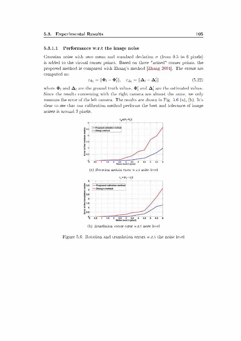
5.3. Experimental Results 105
5.3.1.1 Performance w.r.t the image noise
Gaussian noise with zero mean and standard deviation σ (from 0.5 to 6 pixels)
is added to the virtual corner points. Based on those "noised" corner points, the
proposed method is compared with Zhang's method [Zhang 2004]. The errors are
computed as:
εΦl= ∥Φl −Φ′
l∥, ε∆l= ∥∆l −∆′
l∥ (5.22)
where Φl and ∆l are the ground truth values, Φ′l and ∆′
l are the estimated values.
Since the results concerning with the right camera are almost the same, we only
measure the error of the left camera. The results are shown in Fig. 5.6 (a), (b). It's
clear to see that our calibration method performs the best and tolerance of image
noises is around 3 pixels.
(a) Rotation matrix error w.r.t noise level
(b) Translation vector error w.r.t noise level
Figure 5.6: Rotation and translation errors w.r.t the noise level
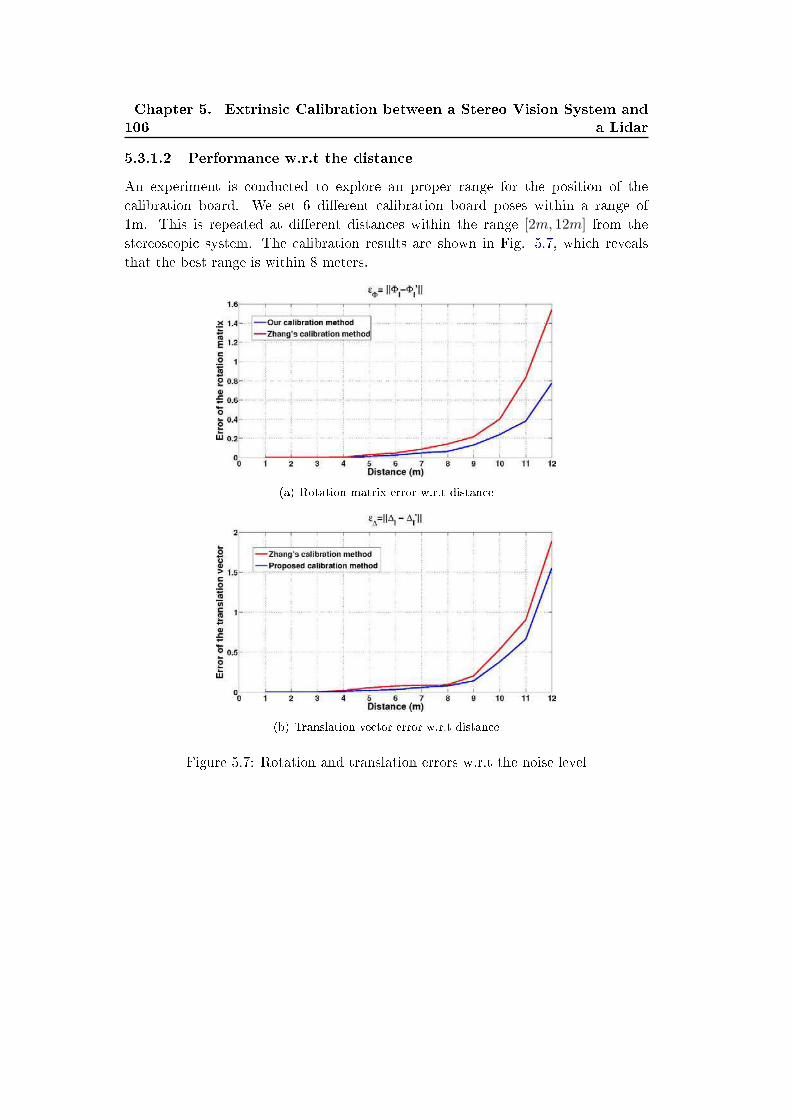
106Chapter 5. Extrinsic Calibration between a Stereo Vision System and
a Lidar
5.3.1.2 Performance w.r.t the distance
An experiment is conducted to explore an proper range for the position of the
calibration board. We set 6 di�erent calibration board poses within a range of
1m. This is repeated at di�erent distances within the range [2m, 12m] from the
stereoscopic system. The calibration results are shown in Fig. 5.7, which reveals
that the best range is within 8 meters.
(a) Rotation matrix error w.r.t distance
(b) Translation vector error w.r.t distance
Figure 5.7: Rotation and translation errors w.r.t the noise level
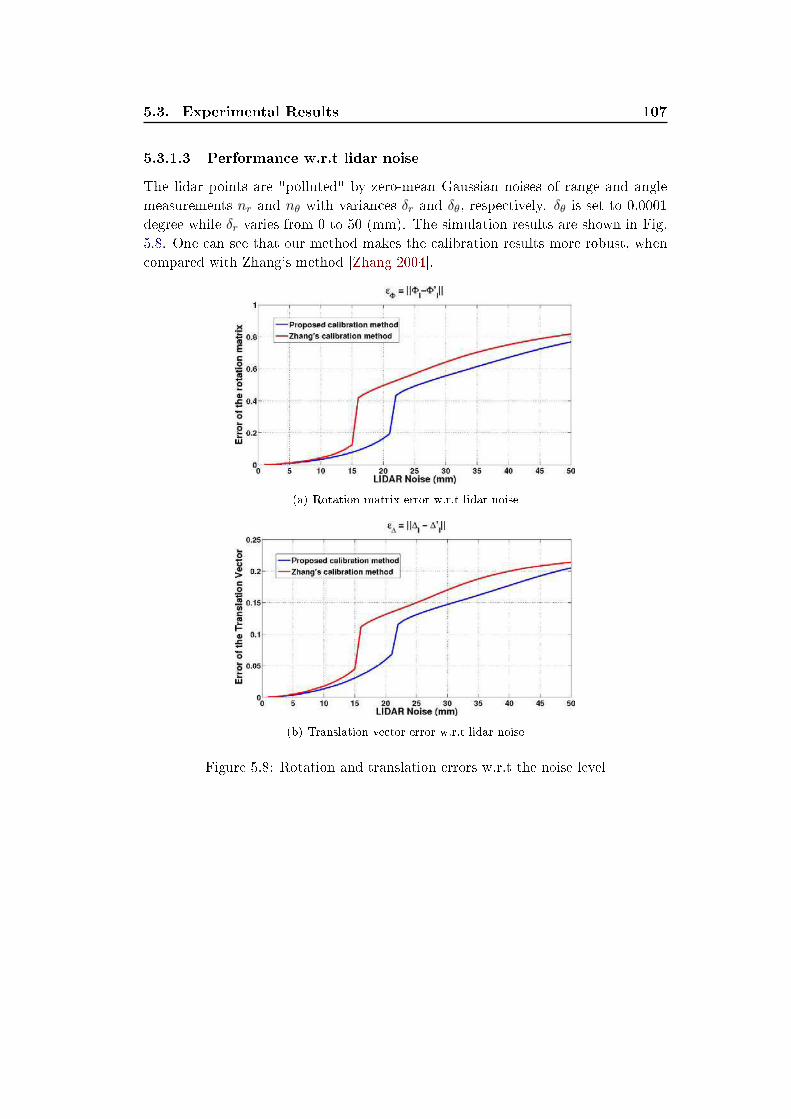
5.3. Experimental Results 107
5.3.1.3 Performance w.r.t lidar noise
The lidar points are "polluted" by zero-mean Gaussian noises of range and angle
measurements nr and nθ with variances δr and δθ, respectively. δθ is set to 0.0001
degree while δr varies from 0 to 50 (mm). The simulation results are shown in Fig.
5.8. One can see that our method makes the calibration results more robust, when
compared with Zhang's method [Zhang 2004].
(a) Rotation matrix error w.r.t lidar noise
(b) Translation vector error w.r.t lidar noise
Figure 5.8: Rotation and translation errors w.r.t the noise level
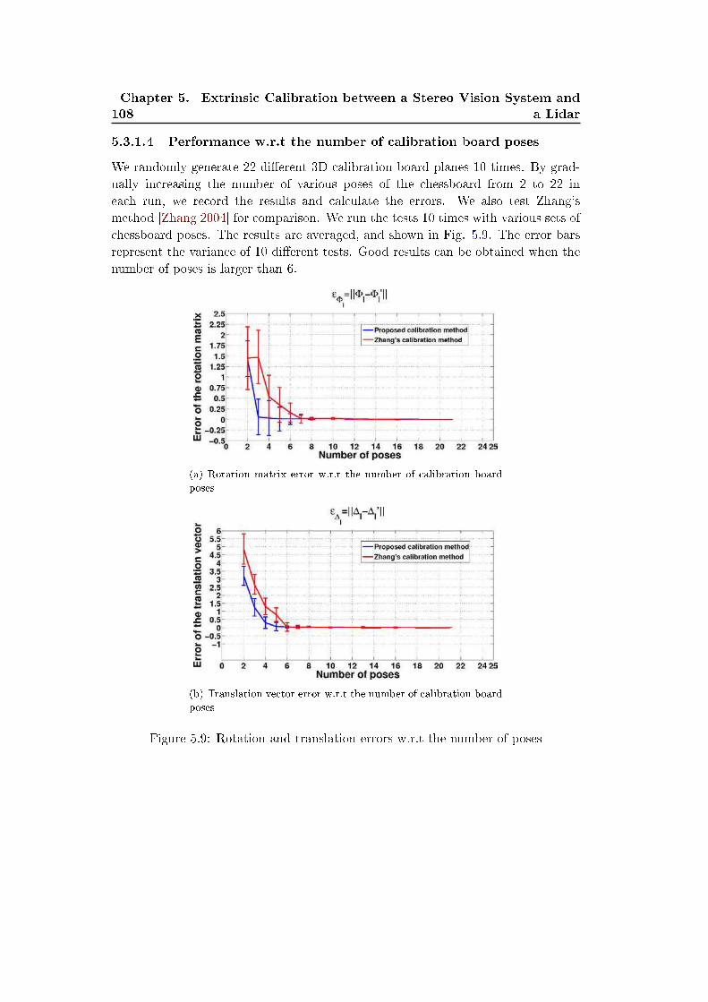
108Chapter 5. Extrinsic Calibration between a Stereo Vision System and
a Lidar
5.3.1.4 Performance w.r.t the number of calibration board poses
We randomly generate 22 di�erent 3D calibration board planes 10 times. By grad-
ually increasing the number of various poses of the chessboard from 2 to 22 in
each run, we record the results and calculate the errors. We also test Zhang's
method [Zhang 2004] for comparison. We run the tests 10 times with various sets of
chessboard poses. The results are averaged, and shown in Fig. 5.9. The error bars
represent the variance of 10 di�erent tests. Good results can be obtained when the
number of poses is larger than 6.
(a) Rotation matrix error w.r.t the number of calibration board
poses
(b) Translation vector error w.r.t the number of calibration board
poses
Figure 5.9: Rotation and translation errors w.r.t the number of poses
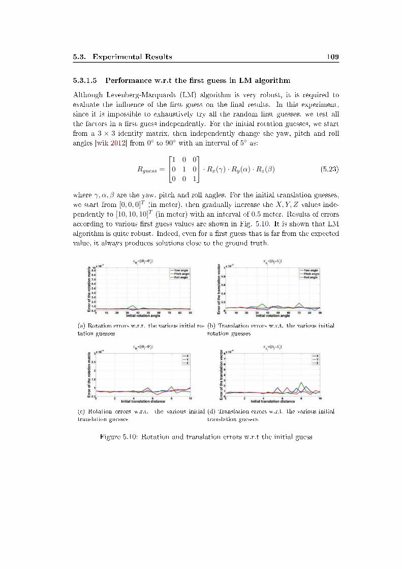
5.3. Experimental Results 109
5.3.1.5 Performance w.r.t the �rst guess in LM algorithm
Although Levenberg-Marquardt (LM) algorithm is very robust, it is required to
evaluate the in�uence of the �rst guess on the �nal results. In this experiment,
since it is impossible to exhaustively try all the random �rst guesses, we test all
the factors in a �rst guess independently. For the initial rotation guesses, we start
from a 3 × 3 identity matrix, then independently change the yaw, pitch and roll
angles [wik 2012] from 0◦ to 90◦ with an interval of 5◦ as:
Rguess =
1 0 0
0 1 0
0 0 1
·Rx(γ) ·Ry(α) ·Rz(β) (5.23)
where γ, α, β are the yaw, pitch and roll angles. For the initial translation guesses,
we start from [0, 0, 0]T (in meter), then gradually increase the X,Y, Z values inde-
pendently to [10, 10, 10]T (in meter) with an interval of 0.5 meter. Results of errors
according to various �rst guess values are shown in Fig. 5.10. It is shown that LM
algorithm is quite robust. Indeed, even for a �rst guess that is far from the expected
value, it always produces solutions close to the ground truth.
(a) Rotation errors w.r.t. the various initial ro-
tation guesses
(b) Translation errors w.r.t. the various initial
rotation guesses
(c) Rotation errors w.r.t. the various initial
translation guesses
(d) Translation errors w.r.t. the various initial
translation guesses
Figure 5.10: Rotation and translation errors w.r.t the initial guess
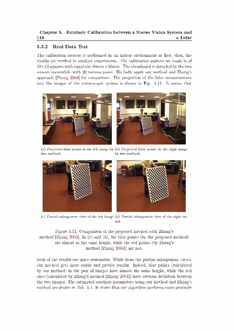
110Chapter 5. Extrinsic Calibration between a Stereo Vision System and
a Lidar
5.3.2 Real Data Test
The calibration process is performed in an indoor environment at �rst, then, the
results are veri�ed in outdoor experiments. The calibration pattern we made is of
19×12 squares with equal size 50mm×50mm. The chessboard is detected by the two
sensors meanwhile with 20 various poses. We both apply our method and Zhang's
approach [Zhang 2004] for comparison. The projection of the lidar measurements
into the images of the stereoscopic system is shown in Fig. 5.11. It seems that
(a) Projected lidar points in the left image by
two methods
(b) Projected lidar points in the right image
by two methods
(c) Partial enlargement view of the left image (d) Partial enlargement view of the right im-
age
Figure 5.11: Comparison of the proposed method with Zhang's
method [Zhang 2004]. In (c) and (d), the blue points (by the proposed method)
are almost at the same height, while the red points (by Zhang's
method [Zhang 2004]) are not.
both of the results are quite reasonable. While from the partial enlargement views,
our method gets more stable and precise results. Indeed, blue points (calculated
by our method) in the pair of images have almost the same height, while the red
ones (calculated by Zhang's method [Zhang 2004]) have obvious deviation between
the two images. The estimated extrinsic parameters using our method and Zhang's
method are shown in Tab. 5.1. It shows that our algorithm performs more precisely
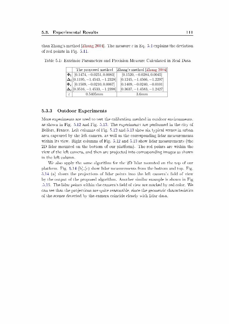
5.3. Experimental Results 111
than Zhang's method [Zhang 2004]. The measure ε in Eq. 5.4 explains the deviation
of red points in Fig. 5.11.
Table 5.1: Extrinsic Parameters and Precision Measure Calculated in Real Data
The proposed method Zhang's method [Zhang 2004]
Φl [0.1474,−0.0251, 0.0083] [0.1520,−0.0284, 0.0045]∆l [0.1195,−1.4543,−1.2328] [0.1245,−1.4566,−1.2297]Φr [0.1509,−0.0210, 0.0067] [0.1409,−0.0240,−0.0101]∆r [0.3516,−1.4533,−1.2398] [0.3637,−1.4583,−1.2427]ε 0.5405mm 3.6mm
5.3.3 Outdoor Experiments
More experiments are used to test the calibration method in outdoor environments,
as shown in Fig. 5.12 and Fig. 5.13. The experiments are performed in the city of
Belfort, France. Left columns of Fig. 5.12 and 5.13 show six typical scenes in urban
area captured by the left camera, as well as the corresponding lidar measurements
within its view. Right columns of Fig. 5.12 and 5.13 show lidar measurements (the
2D lidar mounted on the bottom of our platform). The red points are within the
view of the left camera, and then are projected into corresponding images as shown
in the left column.
We also apply the same algorithm for the 2D lidar mounted on the top of our
platform. Fig. 5.14 (b),(c) show lidar measurements from the bottom and top. Fig.
5.14 (a) shows the projections of lidar points into the left camera's �eld of view
by the output of the proposed algorithm. Another similar example is shown in Fig
.5.15. The lidar points within the camera's �eld of view are marked by red color. We
can see that the projections are quite reasonable, since the geometric characteristics
of the scenes detected by the camera coincide closely with lidar data.
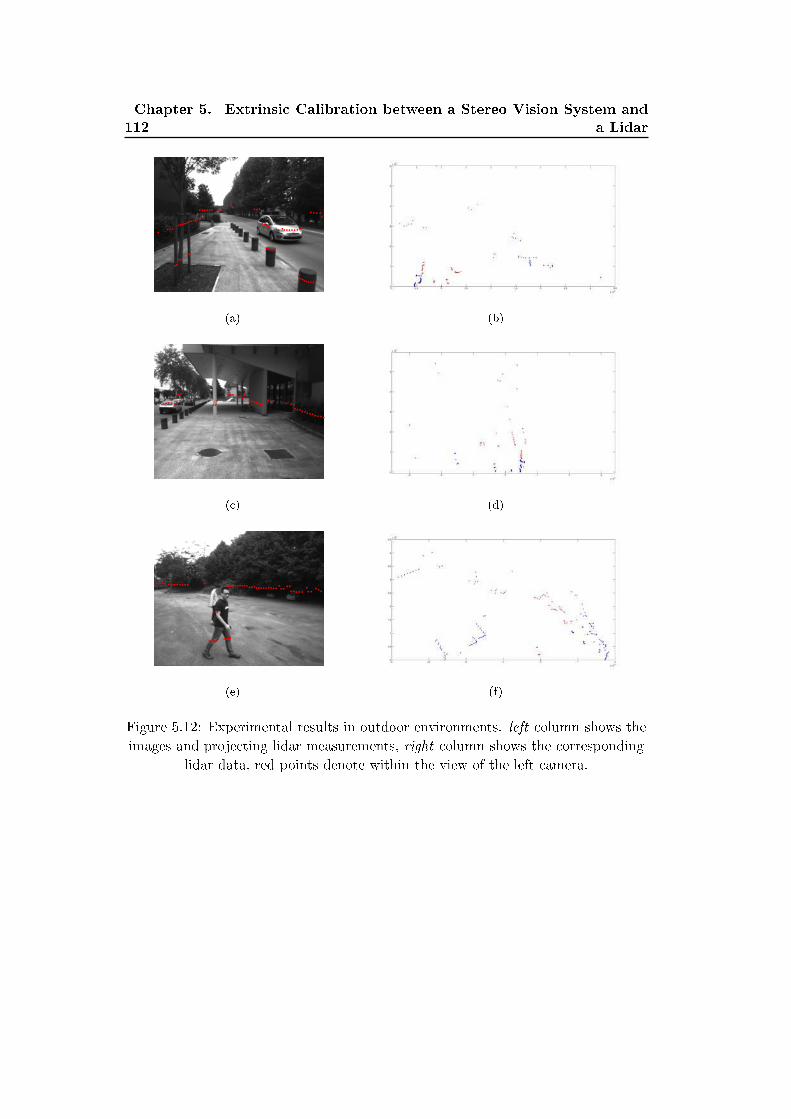
112Chapter 5. Extrinsic Calibration between a Stereo Vision System and
a Lidar
(a) (b)
(c) (d)
(e) (f)
Figure 5.12: Experimental results in outdoor environments. left column shows the
images and projecting lidar measurements, right column shows the corresponding
lidar data, red points denote within the view of the left camera.
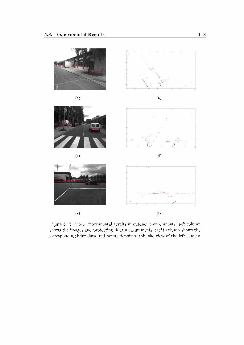
5.3. Experimental Results 113
(a) (b)
(c) (d)
(e) (f)
Figure 5.13: More Experimental results in outdoor environments. left column
shows the images and projecting lidar measurements, right column shows the
corresponding lidar data, red points denote within the view of the left camera.
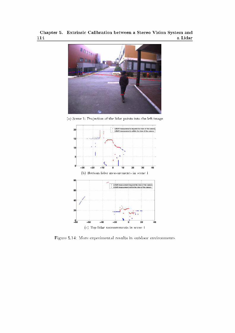
114Chapter 5. Extrinsic Calibration between a Stereo Vision System and
a Lidar
(a) Scene 1: Projection of the lidar points into the left image
(b) Bottom lidar measurements in scene 1
(c) Top lidar measurements in scene 1
Figure 5.14: More experimental results in outdoor environments
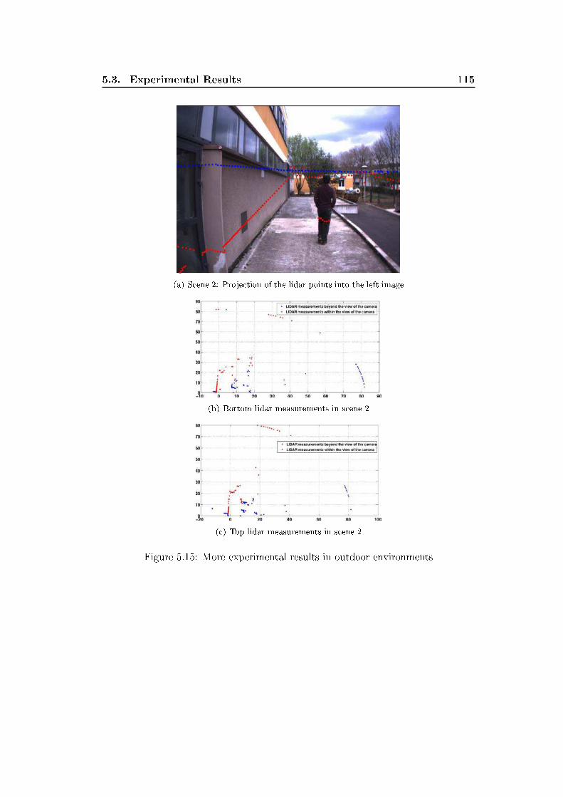
5.3. Experimental Results 115
(a) Scene 2: Projection of the lidar points into the left image
(b) Bottom lidar measurements in scene 2
(c) Top lidar measurements in scene 2
Figure 5.15: More experimental results in outdoor environments

116Chapter 5. Extrinsic Calibration between a Stereo Vision System and
a Lidar
5.4 Conclusion And Future Work
In this chapter, we presented a novel extrinsic calibration method for integrating a
lidar and a binocular stereoscopic system. Since the geometric relationship between
the two cameras in the stereoscopic system is considered, real data experiments
showed that our method is more exact and precise than Zhang's method which is
widely used. Meanwhile, the introduction of sensor noise models and non-linear Ma-
halanobis distance optimization makes our method much more robust than Zhang's
method. This is veri�ed by computer simulation results. The described method
can be applied for any multi-sensor fusion system consisting of multiple cameras
and multiple lidars. Future work will be mainly focused on the calibration of a
stereovision system with multi-layer lidars. Also, we plan to develop an improved
self-calibration method.

Chapter 6
Occupancy Grid Mapping of
Environments
Contents
6.1 Occupancy Grid Mapping by Stereo Vision . . . . . . . . . . 120
6.1.1 Introduction . . . . . . . . . . . . . . . . . . . . . . . . . . . 120
6.1.2 Foundations . . . . . . . . . . . . . . . . . . . . . . . . . . . . 121
6.1.3 Ground Plane Analysis . . . . . . . . . . . . . . . . . . . . . 122
6.1.4 Building Occupancy Grid Map . . . . . . . . . . . . . . . . . 128
6.1.5 Experimental Results of Stereo Vision based Dynamic Occu-
pancy Grid Mapping . . . . . . . . . . . . . . . . . . . . . . . 131
6.2 Occupancy Grid Mapping by Lidar . . . . . . . . . . . . . . . 136
6.2.1 Introduction . . . . . . . . . . . . . . . . . . . . . . . . . . . 136
6.2.2 Ray Casting . . . . . . . . . . . . . . . . . . . . . . . . . . . . 136
6.2.3 Lidar Inverse Model . . . . . . . . . . . . . . . . . . . . . . . 137
6.2.4 Experimental Results . . . . . . . . . . . . . . . . . . . . . . 139
6.3 Occupancy Grid Mapping by Fusing Lidar and Stereo Vision142
6.3.1 Introduction . . . . . . . . . . . . . . . . . . . . . . . . . . . 142
6.3.2 Fusing by Linear Opinion Pool . . . . . . . . . . . . . . . . . 142
6.3.3 Experimental Results . . . . . . . . . . . . . . . . . . . . . . 144
6.4 Conclusion and Future Works . . . . . . . . . . . . . . . . . . 148
In the �eld of intelligent vehicles, many tasks, such as localization, collision
avoidance, path planning, are usually performed based on well represented maps
[Leonard 2008,Nguyen 2012]. Mapping is the process of transforming sensor mea-
surement to an image of the environment. In the early days of robotic research,
many tasks, such as localization/navigation, depend on the map being de�ned as a
�nite sized set of landmarks. However, physical sensors do not usually detect land-
marks unambiguously. In order to use landmark based algorithms, sensor readings
must be pre-processed in a separate step to convert the raw sensor data into a set
of detected landmarks, such as in [Leonard 1991]. The additional step introduces
more error into any algorithm, as well as discarding much of the sensor information
which does not contain any landmark.
One of the primary drawbacks of landmark based maps is data association prob-
lem. Because raw sensor data are not labelled with correct landmarks detected, the
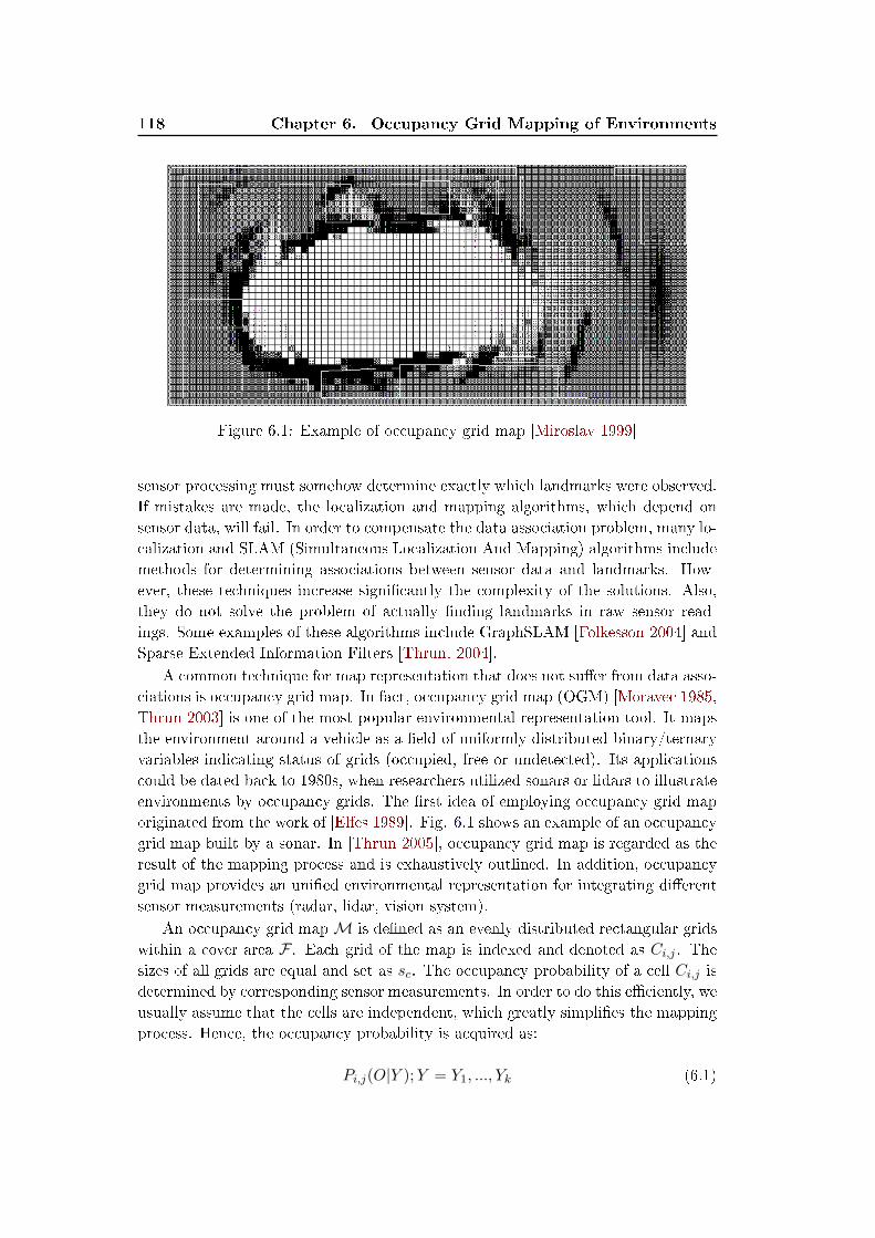
118 Chapter 6. Occupancy Grid Mapping of Environments
Figure 6.1: Example of occupancy grid map [Miroslav 1999]
sensor processing must somehow determine exactly which landmarks were observed.
If mistakes are made, the localization and mapping algorithms, which depend on
sensor data, will fail. In order to compensate the data association problem, many lo-
calization and SLAM (Simultaneous Localization And Mapping) algorithms include
methods for determining associations between sensor data and landmarks. How-
ever, these techniques increase signi�cantly the complexity of the solutions. Also,
they do not solve the problem of actually �nding landmarks in raw sensor read-
ings. Some examples of these algorithms include GraphSLAM [Folkesson 2004] and
Sparse Extended Information Filters [Thrun. 2004].
A common technique for map representation that does not su�er from data asso-
ciations is occupancy grid map. In fact, occupancy grid map (OGM) [Moravec 1985,
Thrun 2003] is one of the most popular environmental representation tool. It maps
the environment around a vehicle as a �eld of uniformly distributed binary/ternary
variables indicating status of grids (occupied, free or undetected). Its applications
could be dated back to 1980s, when researchers utilized sonars or lidars to illustrate
environments by occupancy grids. The �rst idea of employing occupancy grid map
originated from the work of [Elfes 1989]. Fig. 6.1 shows an example of an occupancy
grid map built by a sonar. In [Thrun 2005], occupancy grid map is regarded as the
result of the mapping process and is exhaustively outlined. In addition, occupancy
grid map provides an uni�ed environmental representation for integrating di�erent
sensor measurements (radar, lidar, vision system).
An occupancy grid mapM is de�ned as an evenly distributed rectangular grids
within a cover area F . Each grid of the map is indexed and denoted as Ci,j . The
sizes of all grids are equal and set as sc. The occupancy probability of a cell Ci,j is
determined by corresponding sensor measurements. In order to do this e�ciently, we
usually assume that the cells are independent, which greatly simpli�es the mapping
process. Hence, the occupancy probability is acquired as:
Pi,j(O|Y );Y = Y1, ..., Yk (6.1)
119
where Y denotes all the possible measurements that can be associated to cell Ci,j .
This chapter presents a framework to create occupancy grid maps in a dynamic
environment, based on a stereo vision system and a single layer lidar. Furthermore, a
fusion method to take advantages of the two sensors is presented. It has to be noted
that, in previous researches [Moravec 1985,Thrun 2003], occupancy grid mapping is
produced in a relatively �xed environment (such as rooms, buildings) for a mobile
robot. After generating a global map, it is stored for afterward usage. Under these
circumstances, it is reasonable to build a global map or perform SLAM, since the
robot moves in a closed loop. Whereas the situation changes in the applications
of intelligent vehicle. In our application, the intelligent vehicle has to self-drive
successfully in a dynamic unknown urban area. Therefore, the vehicle faces an
open, unknown and dynamic environment. It emphasizes the ability of mapping
in dynamic environments in real time without prior information. In our works, we
do not address SLAM but try to separate mapping and localization as two tasks.
Hence, the occupancy grid mapping techniques that will be presented in this chapter
are about building a current local map.
The chapter is organized as follows: Sec. 6.1 proposes an occupancy grid map-
ping method by stereo vision. In Sec. 6.2, we describe lidar based occupancy grid
mapping method. At last, a fusion of lidar and stereo vision system to build occu-
pancy grid map is presented in Sec. 6.3
120 Chapter 6. Occupancy Grid Mapping of Environments
6.1 Occupancy Grid Mapping by Stereo Vision
6.1.1 Introduction
In literature, range sensors, such as lidar and radar are usually used for creating
occupancy grid maps. The characteristic of measuring distance directly makes oc-
cupancy grid mapping easy to be performed. Usually, under a given sensor measure-
ment model (such as inverse sensor model [Thrun 2003]), probabilistic occupancy
grid mapping is able to be quickly calculated with the measurements. While in our
application, we also use stereo vision system to observe the surroundings, which
o�ers abundant appearance information. Nevertheless, the di�erent measurement
characteristics of stereo vision system lead to a di�erent processing approach to get
occupancy grid map.
Several existing approaches are listed as follows. In [Murray 2000], the authors
regard stereo sensor as a range �nder, taking the �rst encountered object in each
column as an occupied grid. [Braillon 2006] �rstly estimates ground plane in front
of a stereo-camera, then clusters the detected points above the plane as occupied
grids. Three di�erent types of occupancy grids are analyzed and compared at length
in [Badino 2007], which furthermore proposes three kinds of occupancy likelihood
functions modeled by Gaussian distribution. Quite similar to [Badino 2007], the
method proposed in [Nguyen 2012] introduces an inverse sensor model for stereo-
camera. In [Danescu 2009], occupancy grid map is generated from a digital ele-
vation map after �ltering out road and isle cells according to height information.
In [Perrollaz 2010], the authors directly calculate occupancy grids by several e�ec-
tive probabilistic occupancy grid models in obstacle u-disparity image. In addition,
this method requires a pre-performed road-obstacle separation.
However, many of the aforementioned papers do not treat the problem of mov-
ing objects in dynamic environments. Relied on the motion analysis of a moving
intelligent vehicle (ego-motion estimation, moving object detection and recognition)
described in Chapter. 3, 4, we propose a framework of stereo vision based dynamic
occupancy grid mapping in urban environments. Dynamic occupancy grid map mod-
els real environments by evenly distributed rectangular grids, which contain both
occupancy and motion information. The proposed framework mainly comprises two
components (motion analysis for the vehicle-itself and independent moving objects,
dynamic occupancy grid mapping) within two parallel process (sparse feature points
processing between two consecutive stereo image pairs, dense stereo processing). Fig.
6.2 visualizes the whole framework. For every incoming stereo image pairs, sparse
image feature points are extracted and tracked in a circular manner between the
current and previous image pairs. The successfully tracked feature points are used
to estimate ego-motion of the vehicle itself and independent motions of surrounding
moving objects. Meanwhile, dense stereo disparity is calculated from each stereo
image pair. A pixel-wise moving objects segmentation is performed in U-disparity
map. Finally, the dense stereo information, together with the moving information,
are used to create a dynamic occupancy grid map.
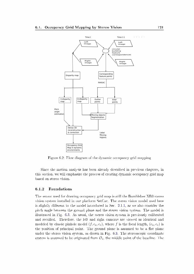
6.1. Occupancy Grid Mapping by Stereo Vision 121
Time t Time t-1
Left
image
Left
Image
Right
image
Right
image
circular
building
feature
correspondences
Disparity mapCorresponding
feature points
RANSAC
Inlier
points
Outlier
points
U-disparity
map
V-disparity
map
Moving objects
Segmentation
Dense 3D
reconstruction
& correction Label Moving regions
Pitch
angle
estimation
Occupancy Grid
Map in dynamic
environments
.....
Figure 6.2: Flow diagram of the dynamic occupancy grid mapping
Since the motion analysis has been already described in previous chapters, in
this section, we will emphasize the process of creating dynamic occupancy grid map
based on stereo vision.
6.1.2 Foundations
The sensor used for drawing occupancy grid map is still the Bumblebee XB3 stereo
vision system installed in our platform SetCar. The stereo vision model used here
is slightly di�erent to the model introduced in Sec. 2.1.1, as we also consider the
pitch angle between the ground plane and the stereo vision system. The model is
illustrated in Fig. 6.3. As usual, the stereo vision system is previously calibrated
and recti�ed. Therefore, the left and right cameras are viewed as identical and
modeled by classic pinhole model (f, cu, cv), where f is the focal length, (cu, cv) is
the position of principal point. The ground plane is assumed to be a �at plane
under the stereo vision system, as drawn in Fig. 6.3. The stereoscopic coordinate
system is assumed to be originated from Os, the middle point of the baseline. The
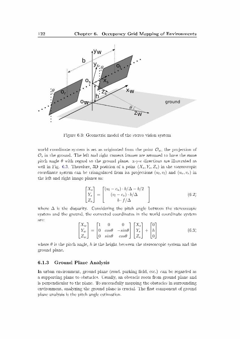
122 Chapter 6. Occupancy Grid Mapping of Environments
b
ow
xw
yw
zw
os
h
Figure 6.3: Geometric model of the stereo vision system
world coordinate system is set as originated from the point Ow, the projection of
Os in the ground. The left and right camera frames are assumed to have the same
pitch angle θ with regard to the ground plane. x-y-z directions are illustrated as
well in Fig. 6.3. Therefore, 3D position of a point (Xs, Ys, Zs) in the stereoscopic
coordinate system can be triangulated from its projections (ul, vl) and (ur, vr) in
the left and right image planes as:
Xs
YsZs
=
(ul − cu) · b/∆− b/2
(vl − cv) · b/∆b · f/∆
(6.2)
where ∆ is the disparity. Considering the pitch angle between the stereoscopic
system and the ground, the corrected coordinates in the world coordinate system
are:
Xw
YwZw
=
1 0 0
0 cosθ −sinθ0 sinθ cosθ
Xs
YsZs
+
0
h
0
(6.3)
where θ is the pitch angle, h is the height between the stereoscopic system and the
ground plane.
6.1.3 Ground Plane Analysis
In urban environment, ground plane (road, parking �eld, etc.) can be regarded as
a supporting plane to obstacles. Usually, an obstacle roots from ground plane and
is perpendicular to the plane. To successfully mapping the obstacles in surrounding
environment, analyzing the ground plane is crucial. The �rst component of ground
plane analysis is the pitch angle estimation.
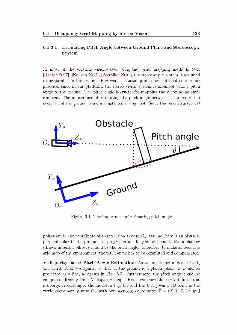
6.1. Occupancy Grid Mapping by Stereo Vision 123
6.1.3.1 Estimating Pitch Angle between Ground Plane and StereoscopicSystem
In most of the existing vision-based occupancy grid mapping methods (e.g.
[Badino 2007], [Nguyen 2012], [Perrollaz 2010]) the stereoscopic system is assumed
to be parallel to the ground. However, this assumption does not hold true in our
practice, since in our platform, the stereo vision system is mounted with a pitch
angle to the ground. The pitch angle is crucial for mapping the surrounding envi-
ronment. The importance of estimating the pitch angle between the stereo vision
system and the ground plane is illustrated in Fig. 6.4. Since the reconstructed 3D
Ground
Obstacle
Pitch angle
Figure 6.4: The importance of estimating pitch angle
points are in the coordinate of stereo vision system Os, assume there is an obstacle
perpendicular to the ground, its projection on the ground plane is like a shadow
(drawn in purple ellipse) caused by the pitch angle. Therefore, to make an accurate
grid map of the environment, the pitch angle has to be computed and compensated.
V-disparity based Pitch Angle Estimation: As we mentioned in Sec. 4.1.2.1,
one attribute of V-disparity is that, if the ground is a planar plane, it would be
projected as a line, as drawn in Fig. 6.5. Furthermore, the pitch angle could be
computed directly from V-disparity map. Here, we show the derivation of this
property. According to the model in Fig. 6.3 and Eq. 6.3, given a 3D point in the
world coordinate system Ow with homogeneous coordinates P = (X,Y, Z, 1)T and
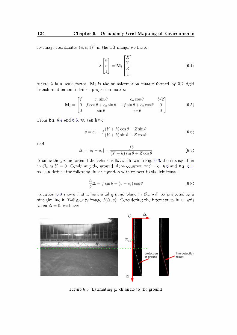
124 Chapter 6. Occupancy Grid Mapping of Environments
its image coordinates (u, v, 1)T in the left image, we have:
λ
u
v
1
= Ml
X
Y
Z
1
(6.4)
where λ is a scale factor, Ml is the transformation matrix formed by 3D rigid
transformation and intrinsic projection matrix:
Ml =
f cu sin θ cu cos θ b/2
0 f cos θ + cv sin θ −f sin θ + cv cos θ 0
0 sin θ cos θ 0
(6.5)
From Eq. 6.4 and 6.5, we can have:
v = cv + f(Y + h) cos θ − Z sin θ
(Y + h) sin θ + Z cos θ(6.6)
and
∆ = |ul − ur| =fb
(Y + h) sin θ + Z cos θ(6.7)
Assume the ground around the vehicle is �at as drawn in Fig. 6.3, then its equation
in Ow is Y = 0. Combining the ground plane equation with Eq. 6.6 and Eq. 6.7,
we can deduce the following linear equation with respect to the left image:
h
b∆ = f sin θ + (v − cv) cos θ (6.8)
Equation 6.8 shows that a horizontal ground plane in Ow will be projected as a
straight line in V-disparity image I(∆, v). Considering the intercept vc in v−axiswhen ∆ = 0, we have:
projection
of ground
line detection
result
Figure 6.5: Estimating pitch angle to the ground
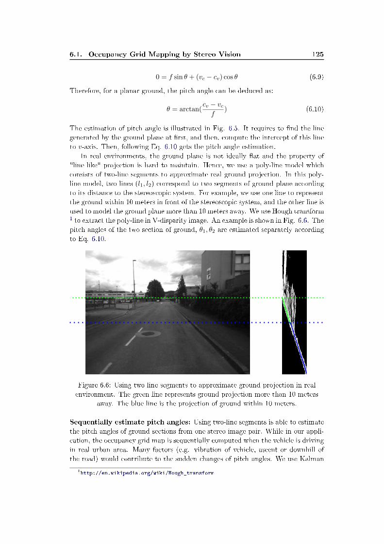
6.1. Occupancy Grid Mapping by Stereo Vision 125
0 = f sin θ + (vc − cv) cos θ (6.9)
Therefore, for a planar ground, the pitch angle can be deduced as:
θ = arctan(cv − vc
f) (6.10)
The estimation of pitch angle is illustrated in Fig. 6.5. It requires to �nd the line
generated by the ground plane at �rst, and then, compute the intercept of this line
to v-axis. Then, following Eq. 6.10 gets the pitch angle estimation.
In real environments, the ground plane is not ideally �at and the property of
"line like" projection is hard to maintain. Hence, we use a poly-line model which
consists of two-line segments to approximate real ground projection. In this poly-
line model, two lines (l1, l2) correspond to two segments of ground plane according
to its distance to the stereoscopic system. For example, we use one line to represent
the ground within 10 meters in front of the stereoscopic system, and the other line is
used to model the ground plane more than 10 meters away. We use Hough transform1 to extract the poly-line in V-disparity image. An example is shown in Fig. 6.6. The
pitch angles of the two section of ground, θ1, θ2 are estimated separately according
to Eq. 6.10.
Figure 6.6: Using two line segments to approximate ground projection in real
environment. The green line represents ground projection more than 10 meters
away. The blue line is the projection of ground within 10 meters.
Sequentially estimate pitch angles: Using two-line segments is able to estimate
the pitch angles of ground sections from one stereo image pair. While in our appli-
cation, the occupancy grid map is sequentially computed when the vehicle is driving
in real urban area. Many factors (e.g. vibration of vehicle, ascent or downhill of
the road) would contribute to the sudden changes of pitch angles. We use Kalman
1http://en.wikipedia.org/wiki/Hough_transform
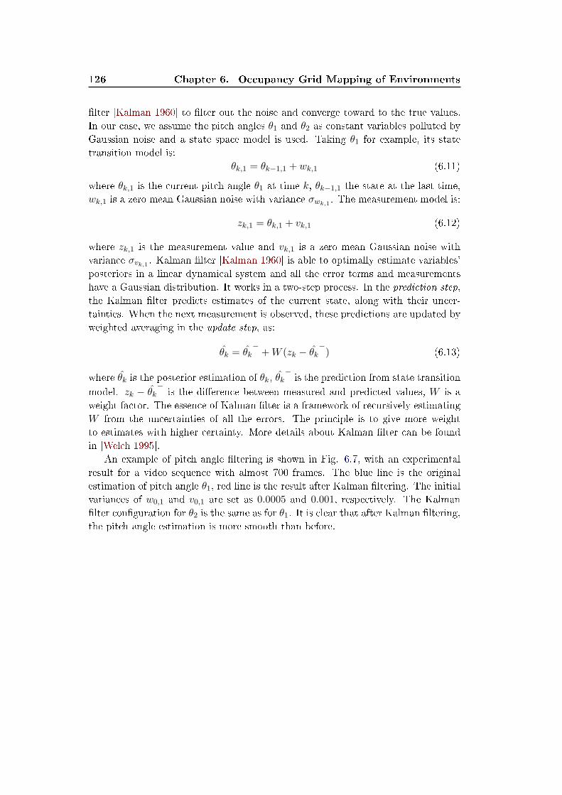
126 Chapter 6. Occupancy Grid Mapping of Environments
�lter [Kalman 1960] to �lter out the noise and converge toward to the true values.
In our case, we assume the pitch angles θ1 and θ2 as constant variables polluted by
Gaussian noise and a state space model is used. Taking θ1 for example, its state
transition model is:
θk,1 = θk−1,1 + wk,1 (6.11)
where θk,1 is the current pitch angle θ1 at time k, θk−1,1 the state at the last time,
wk,1 is a zero mean Gaussian noise with variance σwk,1. The measurement model is:
zk,1 = θk,1 + vk,1 (6.12)
where zk,1 is the measurement value and vk,1 is a zero mean Gaussian noise with
variance σvk,1 . Kalman �lter [Kalman 1960] is able to optimally estimate variables'
posteriors in a linear dynamical system and all the error terms and measurements
have a Gaussian distribution. It works in a two-step process. In the prediction step,
the Kalman �lter predicts estimates of the current state, along with their uncer-
tainties. When the next measurement is observed, these predictions are updated by
weighted averaging in the update step, as:
θk = θk−+W (zk − θk
−) (6.13)
where θk is the posterior estimation of θk, θk−is the prediction from state transition
model. zk − θk−
is the di�erence between measured and predicted values, W is a
weight factor. The essence of Kalman �lter is a framework of recursively estimating
W from the uncertainties of all the errors. The principle is to give more weight
to estimates with higher certainty. More details about Kalman �lter can be found
in [Welch 1995].
An example of pitch angle �ltering is shown in Fig. 6.7, with an experimental
result for a video sequence with almost 700 frames. The blue line is the original
estimation of pitch angle θ1, red line is the result after Kalman �ltering. The initial
variances of w0,1 and v0,1 are set as 0.0005 and 0.001, respectively. The Kalman
�lter con�guration for θ2 is the same as for θ1. It is clear that after Kalman �ltering,
the pitch angle estimation is more smooth than before.
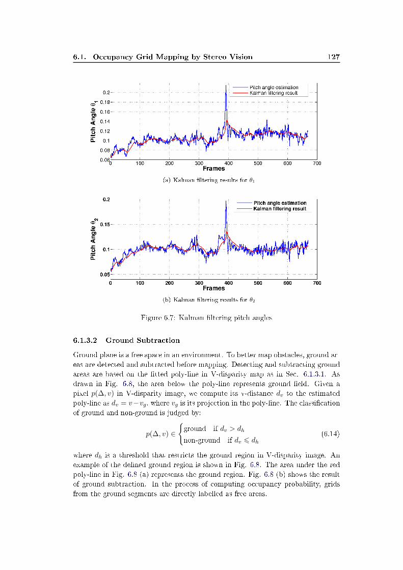
6.1. Occupancy Grid Mapping by Stereo Vision 127
(a) Kalman �ltering results for θ1
(b) Kalman �ltering results for θ2
Figure 6.7: Kalman �ltering pitch angles
6.1.3.2 Ground Subtraction
Ground plane is a free space in an environment. To better map obstacles, ground ar-
eas are detected and subtracted before mapping. Detecting and subtracting ground
areas are based on the �tted poly-line in V-disparity map as in Sec. 6.1.3.1. As
drawn in Fig. 6.8, the area below the poly-line represents ground �eld. Given a
pixel p(∆, v) in V-disparity image, we compute its v-distance dv to the estimated
poly-line as dv = v−vg, where vg is its projection in the poly-line. The classi�cation
of ground and non-ground is judged by:
p(∆, v) ∈{
ground if dv > dh
non-ground if dv ⩽ dh(6.14)
where dh is a threshold that restricts the ground region in V-disparity image. An
example of the de�ned ground region is shown in Fig. 6.8. The area under the red
poly-line in Fig. 6.8 (a) represents the ground region. Fig. 6.8 (b) shows the result
of ground subtraction. In the process of computing occupancy probability, grids
from the ground segments are directly labelled as free areas.
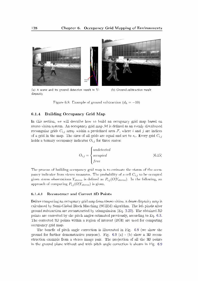
128 Chapter 6. Occupancy Grid Mapping of Environments
Ground
area
(a) A scene and its ground detection result in V-
disparity
(b) Ground subtraction result
Figure 6.8: Example of ground subtraction (dh = −10)
6.1.4 Building Occupancy Grid Map
In this section, we will describe how to build an occupancy grid map based on
stereo vision system. An occupancy grid mapM is de�ned as an evenly distributed
rectangular grids Ci,j array within a prede�ned area F , where i and j are indices
of a grid in the map. The sizes of all grids are equal and set to sc. Every grid Ci,j
holds a ternary occupancy indicator Oi,j for three states:
Oi,j =
undetected
occupied
free
(6.15)
The process of building occupancy grid map is to estimate the status of the occu-
pancy indicator from stereo measures. The probability of a cell Ci,j to be occupied
given stereo observations Ystereo is de�ned as Pi,j(O|Ystereo). In the following, an
approach of computing Pi,j(O|Ystereo) is given.
6.1.4.1 Reconstruct and Correct 3D Points
Before computing an occupancy grid map from stereo vision, a dense disparity map is
calculated by Semi-Global Block Matching (SGBM) algorithm. The left pixels after
ground subtraction are reconstructed by triangulation (Eq. 2.23). The obtained 3D
points are corrected by the pitch angles estimated previously, according to Eq. 6.3.
The corrected 3D points within a region of interest (ROI) are used for computing
occupancy grid map.
The bene�t of pitch angle correction is illustrated in Fig. 6.9 (we show the
ground for further demonstrative purpose). Fig. 6.9 (a) - (b) show a 3D recon-
struction example from a stereo image pair. The projection of all the 3D points
in the ground plane without and with pitch angle correction is shown in Fig. 6.9
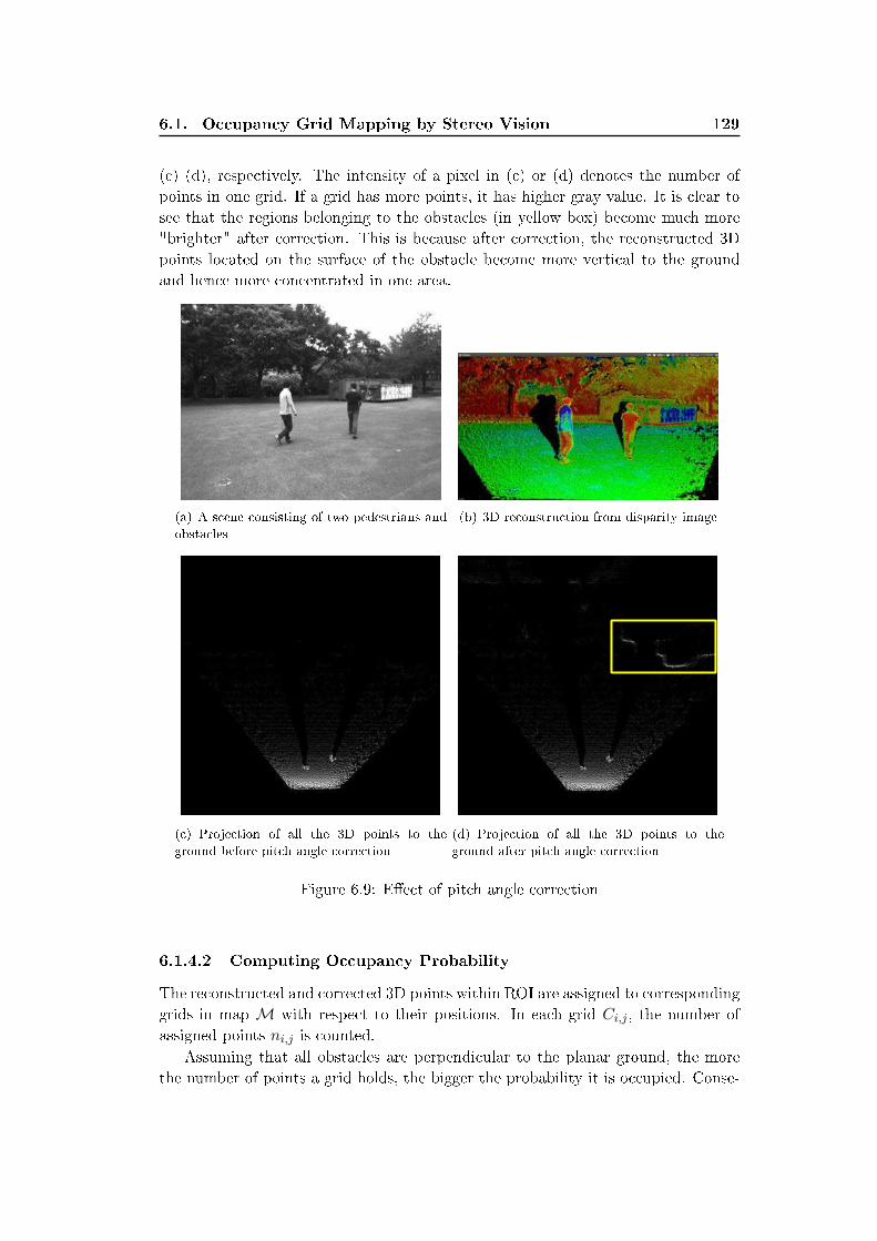
6.1. Occupancy Grid Mapping by Stereo Vision 129
(c) (d), respectively. The intensity of a pixel in (c) or (d) denotes the number of
points in one grid. If a grid has more points, it has higher gray value. It is clear to
see that the regions belonging to the obstacles (in yellow box) become much more
"brighter" after correction. This is because after correction, the reconstructed 3D
points located on the surface of the obstacle become more vertical to the ground
and hence more concentrated in one area.
(a) A scene consisting of two pedestrians and
obstacles
(b) 3D reconstruction from disparity image
(c) Projection of all the 3D points to the
ground before pitch angle correction
(d) Projection of all the 3D points to the
ground after pitch angle correction
Figure 6.9: E�ect of pitch angle correction
6.1.4.2 Computing Occupancy Probability
The reconstructed and corrected 3D points within ROI are assigned to corresponding
grids in map M with respect to their positions. In each grid Ci,j , the number of
assigned points ni,j is counted.
Assuming that all obstacles are perpendicular to the planar ground, the more
the number of points a grid holds, the bigger the probability it is occupied. Conse-
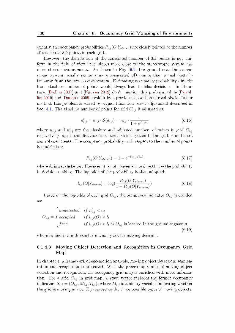
130 Chapter 6. Occupancy Grid Mapping of Environments
quently, the occupancy probabilities Pi,j(O|Ystereo) are closely related to the number
of associated 3D points in each grid.
However, the distribution of the associated number of 3D points is not uni-
form in the �eld of view: the places more close to the stereoscopic system has
more stereo measurements. As shown in Fig. 6.9, the ground near the stereo-
scopic system usually contains more associated 3D points than a real obstacle
far away from the stereoscopic system. Estimating occupancy probability directly
from absolute number of points would always lead to false decisions. In litera-
ture, [Badino 2007] and [Nguyen 2012] don't mention this problem, while [Perrol-
laz 2010] and [Danescu 2009] avoid it by a previous separation of road pixels. In our
method, this problem is solved by sigmoid function based adjustment described in
Sec. 4.1. The absolute number of points for grid Ci,j is adjusted as:
n′i,j = ni,j · S(di,j) = ni,j ·
r
1 + edi,j∗c(6.16)
where ni,j and n′i,j are the absolute and adjusted numbers of points in grid Ci,j
respectively. di,j is the distance from stereo vision system to the grid. r and c are
control coe�cients. The occupancy probability with respect to the number of points
is modeled as:
Pi,j(O|Ystereo) = 1− e−(n′
i.j/δn) (6.17)
where δn is a scale factor. However, it is not convenient to directly use the probability
in decision making. The log-odds of the probability is then adopted:
li,j(O|Ystereo) = log(Pi,j(O|Ystereo)
1− Pi,j(O|Ystereo)) (6.18)
Based on the log-odds of each grid Ci,j , the occupancy indicator Oi,j is decided
as:
Oi,j =
undetected if n′i,j < nt
occupied if li,j(O) ≥ lt
free if li,j(O) < lt or Oi,j is located in the ground segments
(6.19)
where nt and lt are thresholds manually set for making decision.
6.1.4.3 Moving Object Detection and Recognition in Occupancy GridMap
In chapter 4, a framework of ego-motion analysis, moving object detection, segmen-
tation and recognition is presented. With the processing results of moving object
detection and recognition, the occupancy grid map is enriched with more informa-
tion. For a grid Ci,j in grid map, a state vector replaces the former occupancy
indicator: Si,j = (Oi,j ,Mi,j , Ti,j), where Mi,j is a binary variable indicating whether
the grid is moving or not, Ti,j represents the three possible types of moving objects,
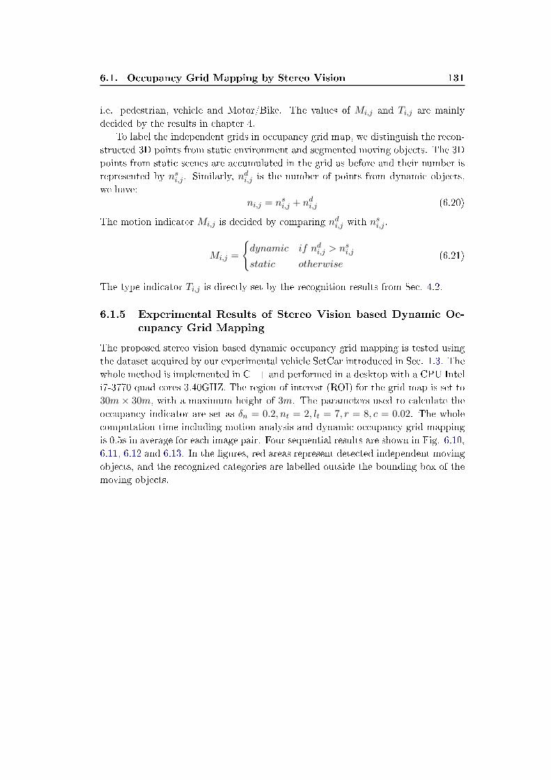
6.1. Occupancy Grid Mapping by Stereo Vision 131
i.e. pedestrian, vehicle and Motor/Bike. The values of Mi,j and Ti,j are mainly
decided by the results in chapter 4.
To label the independent grids in occupancy grid map, we distinguish the recon-
structed 3D points from static environment and segmented moving objects. The 3D
points from static scenes are accumulated in the grid as before and their number is
represented by nsi,j . Similarly, nd
i,j is the number of points from dynamic objects,
we have:
ni,j = nsi,j + nd
i,j (6.20)
The motion indicator Mi,j is decided by comparing ndi,j with ns
i,j .
Mi,j =
{
dynamic if ndi,j > ns
i,j
static otherwise(6.21)
The type indicator Ti,j is directly set by the recognition results from Sec. 4.2.
6.1.5 Experimental Results of Stereo Vision based Dynamic Oc-
cupancy Grid Mapping
The proposed stereo vision based dynamic occupancy grid mapping is tested using
the dataset acquired by our experimental vehicle SetCar introduced in Sec. 1.3. The
whole method is implemented in C++ and performed in a desktop with a CPU Intel
i7-3770 quad cores 3.40GHZ. The region of interest (ROI) for the grid map is set to
30m × 30m, with a maximum height of 3m. The parameters used to calculate the
occupancy indicator are set as δn = 0.2, nt = 2, lt = 7, r = 8, c = 0.02. The whole
computation time including motion analysis and dynamic occupancy grid mapping
is 0.5s in average for each image pair. Four sequential results are shown in Fig. 6.10,
6.11, 6.12 and 6.13. In the �gures, red areas represent detected independent moving
objects, and the recognized categories are labelled outside the bounding box of the
moving objects.
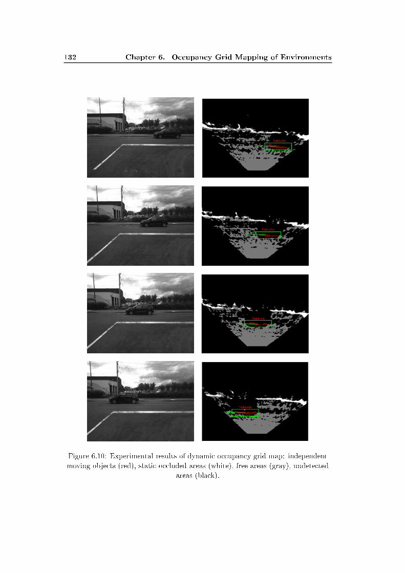
132 Chapter 6. Occupancy Grid Mapping of Environments
Figure 6.10: Experimental results of dynamic occupancy grid map: independent
moving objects (red), static occluded areas (white), free areas (gray), undetected
areas (black).
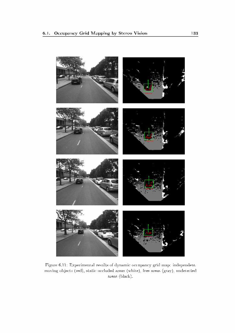
6.1. Occupancy Grid Mapping by Stereo Vision 133
Figure 6.11: Experimental results of dynamic occupancy grid map: independent
moving objects (red), static occluded areas (white), free areas (gray), undetected
areas (black).
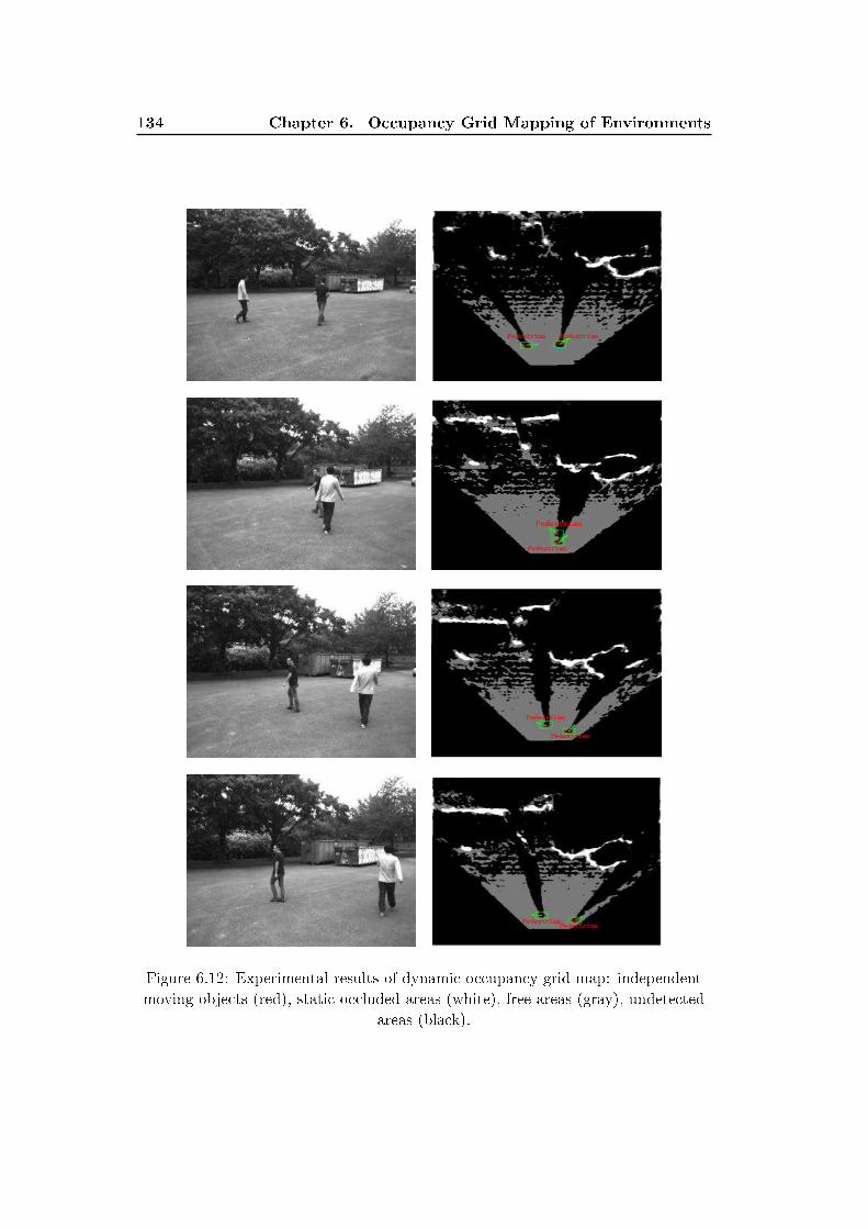
134 Chapter 6. Occupancy Grid Mapping of Environments
Figure 6.12: Experimental results of dynamic occupancy grid map: independent
moving objects (red), static occluded areas (white), free areas (gray), undetected
areas (black).
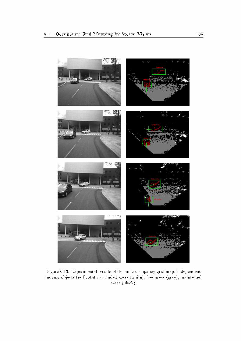
6.1. Occupancy Grid Mapping by Stereo Vision 135
Figure 6.13: Experimental results of dynamic occupancy grid map: independent
moving objects (red), static occluded areas (white), free areas (gray), undetected
areas (black).
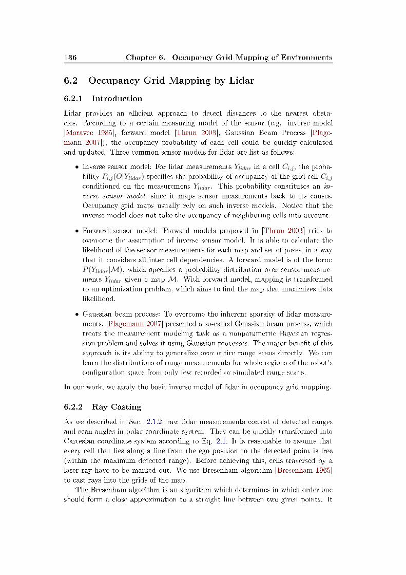
136 Chapter 6. Occupancy Grid Mapping of Environments
6.2 Occupancy Grid Mapping by Lidar
6.2.1 Introduction
Lidar provides an e�cient approach to detect distances to the nearest obsta-
cles. According to a certain measuring model of the sensor (e.g. inverse model
[Moravec 1985], forward model [Thrun 2003], Gaussian Beam Process [Plage-
mann 2007]), the occupancy probability of each cell could be quickly calculated
and updated. Three common sensor models for lidar are list as follows:
• Inverse sensor model: For lidar measurements Ylidar in a cell Ci,j , the proba-
bility Pi,j(O|Ylidar) speci�es the probability of occupancy of the grid cell Ci,j
conditioned on the measurement Ylidar. This probability constitutes an in-
verse sensor model, since it maps sensor measurements back to its causes.
Occupancy grid maps usually rely on such inverse models. Notice that the
inverse model does not take the occupancy of neighboring cells into account.
• Forward sensor model: Forward models proposed in [Thrun 2003] tries to
overcome the assumption of inverse sensor model. It is able to calculate the
likelihood of the sensor measurements for each map and set of poses, in a way
that it considers all inter-cell dependencies. A forward model is of the form:
P (Ylidar|M), which speci�es a probability distribution over sensor measure-
ments Ylidar given a map M. With forward model, mapping is transformed
to an optimization problem, which aims to �nd the map that maximizes data
likelihood.
• Gaussian beam process: To overcome the inherent sparsity of lidar measure-
ments, [Plagemann 2007] presented a so-called Gaussian beam process, which
treats the measurement modeling task as a nonparametric Bayesian regres-
sion problem and solves it using Gaussian processes. The major bene�t of this
approach is its ability to generalize over entire range scans directly. We can
learn the distributions of range measurements for whole regions of the robot's
con�guration space from only few recorded or simulated range scans.
In our work, we apply the basic inverse model of lidar in occupancy grid mapping.
6.2.2 Ray Casting
As we described in Sec. 2.1.2, raw lidar measurements consist of detected ranges
and scan angles in polar coordinate system. They can be quickly transformed into
Cartesian coordinate system according to Eq. 2.1. It is reasonable to assume that
every cell that lies along a line from the ego position to the detected point is free
(within the maximum detected range). Before achieving this, cells traversed by a
laser ray have to be marked out. We use Bresenham algorithm [Bresenham 1965]
to cast rays into the grids of the map.
The Bresenham algorithm is an algorithm which determines in which order one
should form a close approximation to a straight line between two given points. It
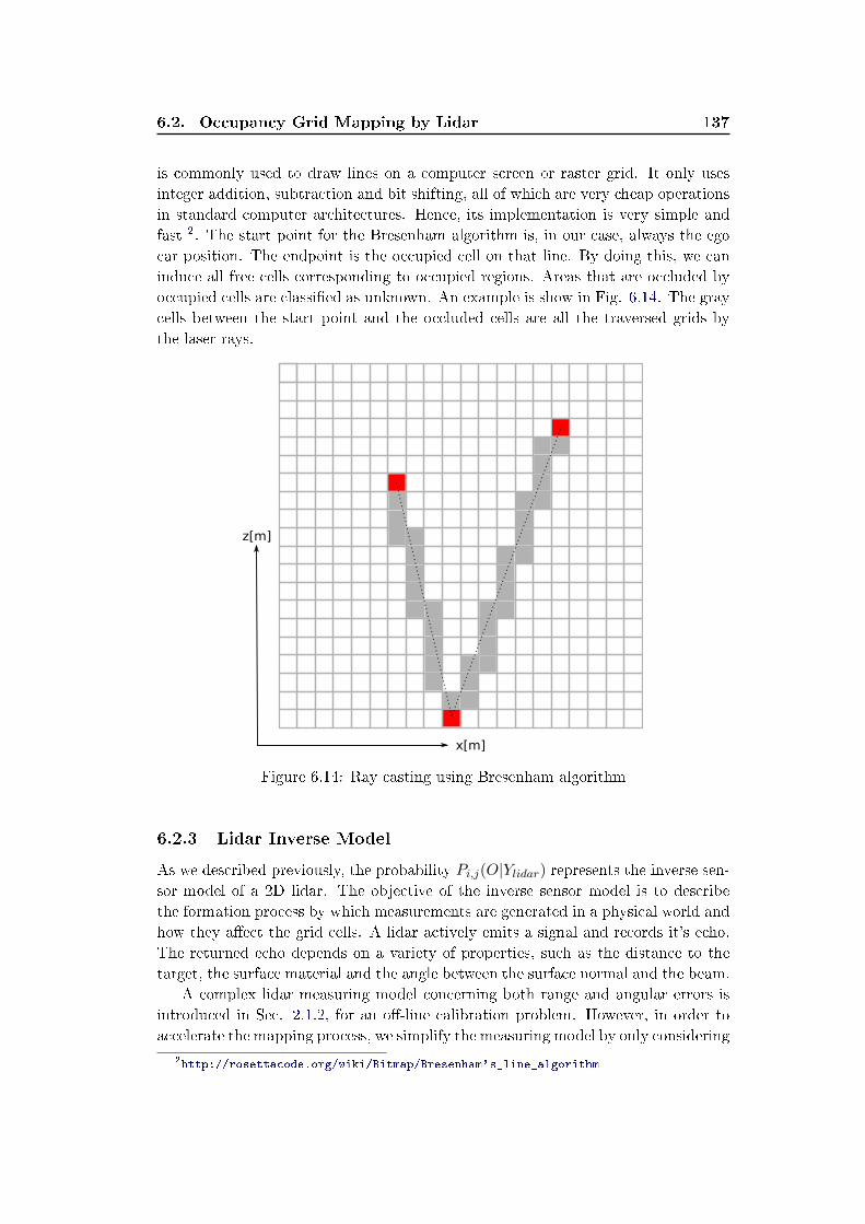
6.2. Occupancy Grid Mapping by Lidar 137
is commonly used to draw lines on a computer screen or raster grid. It only uses
integer addition, subtraction and bit shifting, all of which are very cheap operations
in standard computer architectures. Hence, its implementation is very simple and
fast 2. The start point for the Bresenham algorithm is, in our case, always the ego
car position. The endpoint is the occupied cell on that line. By doing this, we can
induce all free cells corresponding to occupied regions. Areas that are occluded by
occupied cells are classi�ed as unknown. An example is show in Fig. 6.14. The gray
cells between the start point and the occluded cells are all the traversed grids by
the laser rays.
z[m]
x[m]
Figure 6.14: Ray casting using Bresenham algorithm
6.2.3 Lidar Inverse Model
As we described previously, the probability Pi,j(O|Ylidar) represents the inverse sen-sor model of a 2D lidar. The objective of the inverse sensor model is to describe
the formation process by which measurements are generated in a physical world and
how they a�ect the grid cells. A lidar actively emits a signal and records it's echo.
The returned echo depends on a variety of properties, such as the distance to the
target, the surface material and the angle between the surface normal and the beam.
A complex lidar measuring model concerning both range and angular errors is
introduced in Sec. 2.1.2, for an o�-line calibration problem. However, in order to
accelerate the mapping process, we simplify the measuring model by only considering
2http://rosettacode.org/wiki/Bitmap/Bresenham's_line_algorithm
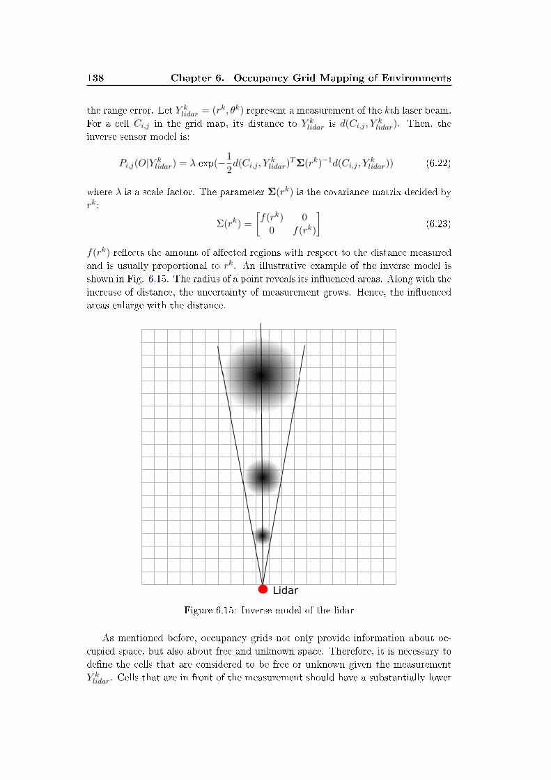
138 Chapter 6. Occupancy Grid Mapping of Environments
the range error. Let Y klidar = (rk, θk) represent a measurement of the kth laser beam.
For a cell Ci,j in the grid map, its distance to Y klidar is d(Ci,j , Y
klidar). Then, the
inverse sensor model is:
Pi,j(O|Y klidar) = λ exp(−1
2d(Ci,j , Y
klidar)
TΣ(rk)−1d(Ci,j , Yklidar)) (6.22)
where λ is a scale factor. The parameter Σ(rk) is the covariance matrix decided by
rk:
Σ(rk) =
[
f(rk) 0
0 f(rk)
]
(6.23)
f(rk) re�ects the amount of a�ected regions with respect to the distance measured
and is usually proportional to rk. An illustrative example of the inverse model is
shown in Fig. 6.15. The radius of a point reveals its in�uenced areas. Along with the
increase of distance, the uncertainty of measurement grows. Hence, the in�uenced
areas enlarge with the distance.
Lidar
Figure 6.15: Inverse model of the lidar
As mentioned before, occupancy grids not only provide information about oc-
cupied space, but also about free and unknown space. Therefore, it is necessary to
de�ne the cells that are considered to be free or unknown given the measurement
Y klidar. Cells that are in front of the measurement should have a substantially lower
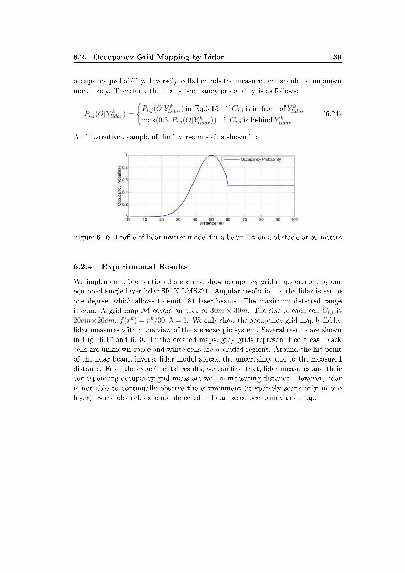
6.2. Occupancy Grid Mapping by Lidar 139
occupancy probability. Inversely, cells behinds the measurement should be unknown
more likely. Therefore, the �nally occupancy probability is as follows:
Pi,j(O|Y klidar) =
{
Pi,j(O|Y klidar) in Eq.6.15 if Ci,j is in front of Y k
lidar
max(0.5, Pi,j(O|Y klidar)) if Ci,j is behind Y k
lidar
(6.24)
An illustrative example of the inverse model is shown in:
Figure 6.16: Pro�le of lidar inverse model for a beam hit on a obstacle at 50 meters
6.2.4 Experimental Results
We implement aforementioned steps and show occupancy grid maps created by our
equipped single layer lidar SICK LMS221. Angular resolution of the lidar is set to
one degree, which allows to emit 181 laser beams. The maximum detected range
is 80m. A grid map M covers an area of 30m × 30m. The size of each cell Ci,j is
20cm×20cm. f(rk) = rk/30, λ = 1. We only show the occupancy grid map build by
lidar measures within the view of the stereoscopic system. Several results are shown
in Fig. 6.17 and 6.18. In the created maps, gray grids represent free areas, black
cells are unknown space and white cells are occluded regions. Around the hit point
of the lidar beam, inverse lidar model spread the uncertainty due to the measured
distance. From the experimental results, we can �nd that, lidar measures and their
corresponding occupancy grid maps are well in measuring distance. However, lidar
is not able to continually observe the environment (it sparsely scans only in one
layer). Some obstacles are not detected in lidar based occupancy grid map.
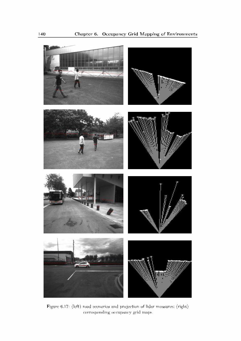
140 Chapter 6. Occupancy Grid Mapping of Environments
Figure 6.17: (left) road scenarios and projection of lidar measures; (right)
corresponding occupancy grid maps
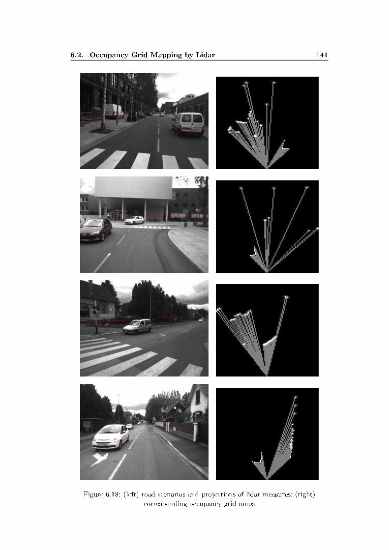
6.2. Occupancy Grid Mapping by Lidar 141
Figure 6.18: (left) road scenarios and projections of lidar measures; (right)
corresponding occupancy grid maps
142 Chapter 6. Occupancy Grid Mapping of Environments
6.3 Occupancy Grid Mapping by Fusing Lidar and
Stereo Vision
6.3.1 Introduction
Standard data fusion methods used for navigation tasks incorporate integration of
data from sets of onboard sensors of the same type, or at least of those based on
similar sensing principles. Typical classes for such sensors are range �nders, data
from other localization systems, etc. As the goal is to achieve maximum robustness
of after fusion data, it is assumed that further improvements might be obtained by
direct integration across di�erent kinds of sensing systems. It is expected that this
will introduce new possibilities in the fusion �eld. The expectation is to bring better
performance through exploring capabilities to combine multiple sources in situations
when some sensors fail. A straightforward candidate for this is direct fusion of range
measuring devices with intensity images. As we stated before, the lidar is superior
to stereoscopic system in distance measuring. In adverse, stereoscopic system pro-
vides more integral appearance descriptions of the environment. In literature, many
methods are proposed to integrate data from lidar and stereoscopic system. These
methods can be roughly divided into two categories:
• Object level fusion. In [Flórez 2011], moving objects are �rstly detected by a
multi-layer lidar. Then, the objects are veri�ed by a stereoscopic system to
improve integrity of a driving assistance system. Similar to this, the method
proposed in [Aycard 2011] seperately detects moving objects by a multi-layer li-
dar and a stereoscopic system. The independently detected objects are merged
for further tracking and classi�cation.
• Map level fusion. In [Stepan 2005], occupancy grid maps are built indepen-
dently by a monocular camera and a lidar. With considering di�erent accuracy
of the two sensors, the combination of them leads to more accurate 2D maps of
the environment. [Moras 2011] proposed a credibilist approach used to model
the sensor information to create occupancy grid map. Con�icting information
are handled by Dempster-Shafer theory. Another fusion model named linear
opinion pools is proposed in [Adarve 2012]. It models the con�dences of lidar
measures and stereo data for integrating them in an occupancy grid map.
6.3.2 Fusing by Linear Opinion Pool
In our application, we choose the linear opinion pool proposed in [DeGroot 1974,
Adarve 2012] to integrate the lidar based and stereo based occupancy grid maps
together. The original idea is to perform fusion as a weighted sum of sensor obser-
vations. The weight is estimated as a con�dence on every sensor's observation. By
combining these con�dences, the opinion of a non reliable sensor is lowered by a low
con�dence and hence, the result of the fusion process will depend on those reliable
sensors which receive a higher weight.
6.3. Occupancy Grid Mapping by Fusing Lidar and Stereo Vision 143
In [Adarve 2012], under the linear opinion pool, the posterior distribution over
the occupancy of a cell Ci,j gives the opinion of m sensors Y1...Ym. Each sensor gives
two quantities: its estimation for the occupancy of the cell Pi,j(O|Yk) and wk(Ci,j),
a measure of the con�dence for such estimations. Under the assumption of mutually
independent cells, the fusion of all sensory information is as follows:
Pi,j(O|Y 1...Y m) = α
m∑
k=1
wk(Ci,j)Pi,j(O|Y k) (6.25)
where α = [∑
k wk(Ci,j)]−1 is a normalization factor for the weights. In our cases,
the sensor measures either come from the lidar or stereoscopic system. Since we have
already got occupancy grid maps from stereo vision system and lidar. Di�erent
to [Adarve 2012], where every measurement from stereoscopic system is assigned
with a weight, we perform the fusion between the lidar measures and occupancy grid
map made by stereoscopic system respectively. Hence, the fusion process becomes:
Pi,j(O|Y 1...Y m) = α
m∑
k=1
wk(Ci,j)Pi,j(O|Y 1lidar...Y
m−1lidar , Y
mstereo) (6.26)
Based on equation 6.26, for each sensor measure Y k (either from lidar or from
stereoscopic system), we have to de�ne P (O|Y k), the probability of a cell being
occupied given the sensor information; and wk(Ci,j), the con�dence on the opinion.
6.3.2.1 Align Lidar with Stereoscopic System
The lidar measures and stereoscopic data are located in two di�erent coordinate
systems, R3stereo and R3
lidar. Before applying a fusion of the data, the measurements
from the two coordinate systems have to be correctly aligned.
The alignment is based on the extrinsic calibration results presented in chapter
5. After the extrinsic calibration, the 3D rigid transformation ϕ,∆ from lidar to
stereoscopic coordinate system is acquired. Hence, before the fusion, all the lidar
measures are transformed into stereoscopic coordinate system according to Eq. 5.3.
Next, we will discuss the models of con�dences.
6.3.2.2 Con�dences of Lidar and Stereoscopic System
The occupancy probability of a cell Ci,j being occupied given the sensor measure-
ment is given by Eq. 6.22 (lidar) or Eq. 6.17 (stereo). The con�dences of the two
kinds of measurements are described as follows.
For the con�dence of a lidar measurement, consider the probability that an
unexpected object is detected before the real hit of the laser beam. This is modeled
by:
wlidar(z, z∗) =
β for z ∈ [0, z∗]
βe−(z−z∗)2
2σ2 forz ∈ (z∗, zmax](6.27)
where z∗ is the detected range, β is the value of occupancy probability at the hit
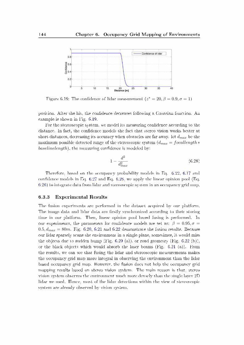
144 Chapter 6. Occupancy Grid Mapping of Environments
Figure 6.19: The con�dence of lidar measurement (z∗ = 20, β = 0.9, σ = 1)
position. After the hit, the con�dence decreases following a Gaussian function. An
example is shown in Fig. 6.19.
For the stereoscopic system, we model its measuring con�dence according to the
distance. In fact, the con�dence models the fact that stereo vision works better at
short distances, decreasing its accuracy when obstacles are far away. let dmax be the
maximum possible detected range of the stereoscopic system (dmax = focallength ∗baselinelength), the measuring con�dence is modeled by:
1− d2
d2max
(6.28)
Therefore, based on the occupancy probability models in Eq. 6.22, 6.17 and
con�dence models in Eq. 6.27 and Eq. 6.28, we apply the linear opinion pool (Eq.
6.26) to integrate data from lidar and stereoscopic system in an occupancy grid map.
6.3.3 Experimental Results
The fusion experiments are performed in the dataset acquired by our platform.
The image data and lidar data are �rstly synchronized according to their storing
time in our platform. Then, linear opinion pool based fusing is performed. In
our experiments, the parameters for con�dence models are set as: β = 0.95, σ =
0.5, dmax = 80m. Fig. 6.20, 6.21 and 6.22 demonstrate the fusion results. Because
our lidar sparsely scans the environment in a single plane, sometimes, it would miss
the objects due to sudden bump (Fig. 6.20 (a)), or road geometry (Fig. 6.22 (b)),
or the black objects which would absorb the laser beams (Fig. 6.21 (a)). From
the results, we can see that fusing the lidar and stereoscopic measurements makes
the occupancy grid map more integral in observing the environment than the lidar
based occupancy grid map. However, the fusion does not help the occupancy grid
mapping results based on stereo vision system. The main reason is that, stereo
vision system observes the environment much more densely than the single layer 2D
lidar we used. Hence, most of the lidar detections within the view of stereoscopic
system are already observed by vision system.
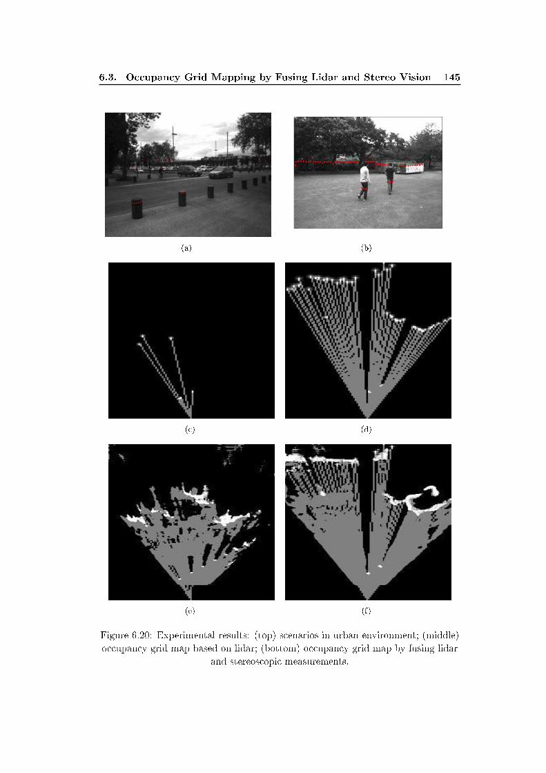
6.3. Occupancy Grid Mapping by Fusing Lidar and Stereo Vision 145
(a) (b)
(c) (d)
(e) (f)
Figure 6.20: Experimental results: (top) scenarios in urban environment; (middle)
occupancy grid map based on lidar; (bottom) occupancy grid map by fusing lidar
and stereoscopic measurements.
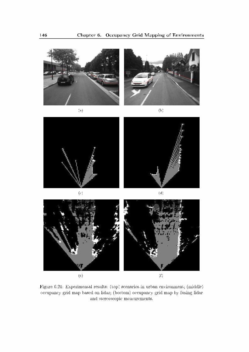
146 Chapter 6. Occupancy Grid Mapping of Environments
(a) (b)
(c) (d)
(e) (f)
Figure 6.21: Experimental results: (top) scenarios in urban environment; (middle)
occupancy grid map based on lidar; (bottom) occupancy grid map by fusing lidar
and stereoscopic measurements.
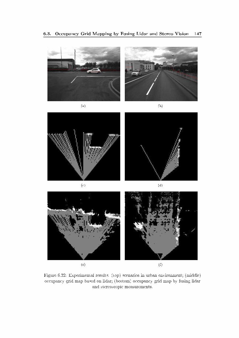
6.3. Occupancy Grid Mapping by Fusing Lidar and Stereo Vision 147
(a) (b)
(c) (d)
(e) (f)
Figure 6.22: Experimental results: (top) scenarios in urban environment; (middle)
occupancy grid map based on lidar; (bottom) occupancy grid map by fusing lidar
and stereoscopic measurements.

148 Chapter 6. Occupancy Grid Mapping of Environments
6.4 Conclusion and Future Works
In this chapter we described a framework of generating occupancy grid map from
stereoscopic system, lidar and combination of both. Stereoscopic based occupancy
grid mapping is achieved by �rstly analyzing ground plane geometric characteristic
(pitch angle) and pixel-wisely subtract ground plane in the image. Next, recon-
structed 3D points are corrected by estimated pitch angles to improve the per-
formance of occupancy grid map. Occupancy probability of each grid is calculated
based on associated 3D points in each grid. In addition, independent moving objects
and their categories are also labelled in the occupancy grid map by the processing
results of chapter 4.
Then, we also create occupancy grid map based on a classic inverse sensor model
of a single layer lidar. Since single layer lidar is not stable in observing the envi-
ronment, we prove that fusing stereo information could improve the quality of oc-
cupancy grid map. However, for the stereo vision based occupancy grid map, fusing
with 2D lidar data does not bring su�cient improvements. The main reason of this
problem is that, in our platform, a single layer 2D lidar is not robust enough to
observe the environment.
For the future works, the current works could be improved by a Bayesian oc-
cupancy �lter that is capable of accurately estimating and tracking the state of
dynamic environments. Also, we intend to further develop tracking method in the
occupancy grid map. To improve the fusion of stereo vision based and lidar based
occupancy grid map, we hope the multi-layer lidar or 3D lidar could be helpful.
Chapter 7
Conclusions and Future Works
7.1 Conclusions
The problems addressed in this thesis concern several basic topics of perception
systems in intelligent vehicles. Perception systems are the eyes of intelligent vehicles,
which are in charge of environment analyzing and understanding. After a review of
basic knowledges used in the thesis, we proposed a series of methods to analyze the
environment.
In the �rst, a stereo vision based ego-motion estimation method is presented in
chapter 3. The stereo vision based visual odometry has been researched for decades.
Hence, we just follow a classic framework shown in Fig. 3.1. Although this frame-
work is relatively stable, in literature, it lacks engineering comparisons of di�erent
image feature detectors, as well as di�erent kinds of feature association methods.
We compare several representative feature detectors and proposed several standards
to choose the suitable feature detectors. In addition, we also compare tracker based
with matching based feature association approaches. From the comparison, we �nd
that CenSURE (or STAR) feature detector with KLT feature tracker achieve the
best performance. The selected approach is tested both in an open dataset and
our dataset. The real experimental results show that, compared with GPS, visual
odometry still lacks accuracy, especially in long distance.
In the second, an independent moving object detection, segmentation and recog-
nition method is proposed in chapter 4. The moving object detection is based on
the results of visual odometry. The outliers discarded by ego-motion estimation are
used for detecting moving objects in U-disparity image. The segmentation is also
performed in U-disparity image by a �ood-�ll algorithm. Then, spatial features of
segmented moving objects are extracted and sent to a pre-trained classi�er for rec-
ognizing three common categories of objects: pedestrian, vehicle and motor/cyclist.
In our proposed method, kernel PCA algorithm is adopted to boost original simple
spatial features by mapping the low dimensional data into high dimensional space.
Several commonly used classi�ers, such as random forest, gradient boost trees are
compared to get the best classi�er. The real experiments show that gradient boost
trees achieve best recognition rate.
In the third, we developed a method to achieve optimal extrinsic calibration
between the stereoscopic system and a 2D lidar using 3D reconstruction from stereo
vision. We improve the accuracy of extrinsic calibration by considering the mea-
suring models of the two sensors. The introduction of sensor models make the
estimation (stereo estimation of 3D planes and �nal estimation of the extrinsic pa-
150 Chapter 7. Conclusions and Future Works
rameters) more precise. The improvement of accuracy is demonstrated by comparing
our method to a popular method.
At last, occupancy grid map, a classic tool of interpreting environment, is built
by stereoscopic system, lidar and fusing them together. For better mapping the en-
vironment by stereoscopic system, we estimate the pitch angle of the ground plane
with regards to the stereoscopic system. The pitch angle compensation greatly im-
prove the quality of occupancy grid map. Furthermore, the moving object detection
and recognition results acquired previously are integrated to enhance the occupancy
grid map. As for a complementary sensor to stereoscopic system, we also create oc-
cupancy grid map from 2D lidar measurements. Then, a linear opinion pool based
fusing method is proposed to integrate the two kinds of measurements into one oc-
cupancy grid map. Real experimental results show that, the fusion improve the
quality of lidar based occupancy grid map. However, the fusion does not improve
the quality of stereo based occupancy grid map, due to 2D lidar's sparse data.
7.2 Future Works
In the author's point of view, many perspectives are envisaged to improve the current
works in the future.
To improve the accuracy of stereo vision based visual odometry, several ap-
proaches could be tried:
• Develop more accurate feature detectors and feature tracking method.
• Improve the accuracy of current feature detector by estimating the sub-pixel
positions.
• Consider fusing the visual odometry with other sensors, such as IMU.
For the independent moving object detection/segmentation/recognition, the pos-
sible improvements maybe:
• Combine the moving object detection with object recognition, which maybe
solve the problem of failure in detecting moving pedestrians.
• Better segmentation method directly performed in raw image should be tried.
The current segmentation in disparity image is not quite satis�ed.
• The extracted spatial features could boost the visual features (HoG, LBP,
Haar). We hope to furthermore improve the recognition results by combining
these two kinds of features.
For the works of calibration, in the future, we plan to introduce more di�erent
sensors, e.g. multi-layer lidar, 3D lidar. Hence, we plan to calibrate a multiple
sensor system.
At last, for the occupancy grid mapping of the environment, the potential im-
provements are:

7.2. Future Works 151
• Bayesian �ltering framework could be implemented to guide the update of the
map in sequence.
• Implement object tracking in the occupancy grid map.
• Semantic environmental interpretation could be added into the occupancy grid
map. For example, we hope to know where is the road, buildings, pedestrians
and vehicles in the map. The semantic information could be either from the
object detectors or semantic image segmentation methods.
• To improve the fusing results of lidar and stereo vision system, ,ore stable and
powerful lidar, such as multi-layer lidar, 3D lidar could replace the original
single layer lidar.
After these possible improvements, an autonomous navigation system is able to
achieved based on the current works. We hope the works presented in the thesis
would be helpful for the following Ph.D students who research in this area.

Appendix A
Publications
Journal:
1. Y. Li, Y. Ruichek and C. Cappelle, "Optimal Extrinsic Calibration between a
Stereoscopic System and a Lidar", in IEEE Transactions on Instrumentation
& Measurements 2013 (IF: 1.3).
Conference:
1. Y. Li, Y. Ruichek, C. Cappelle "3D Triangulation based Extrinsic Calibration
between a Stereo Vision System and a LIDAR", in 14th IEEE International
Conference on Intelligent Transportation Systems (ITSC), Washington D.C.,
USA, 2011.
2. Y. Li, Y. Ruichek "Moving Objects Detection and Recognition Using Sparse
Spacial Information in Urban Environments", in Proc. of IEEE Intelligent
Vehicles Symposium (IVS), Alcala de Henares, Spain, 2012.
3. Y. Li, Y. Ruichek, C. Cappelle "Calibrage Extrinsèque Entre Un Système
Stéréoscopique Et Un Télémètre Laser", In Proc. of Conférence Internationale
Francophone dAutomatique (CIFA 2012), Grenoble, France, 2012.
4. Y. Li, Y. Ruichek and C. Cappelle "Extrinsic Calibration between a Stereo-
scopic System and a Lidar with Sensor Noise Models", in Proc. of IEEE Con-
ference on Multisensor Fusion and Information Integration (MFI), Hamburg,
Germany, 2012.
5. Y. Li, Y. Ruichek "Building Variable Resolution Occupancy Grid Map from
Stereoscopic System - a Quadtree based Approach", in Proc. of IEEE Intelli-
gent Vehicles Symposium (IVS), Gold Coast, Australia, 2013.
6. Y. Li, Y. Ruichek "Observing Dynamic Urban Environment through Stereo-
vision based Dynamic Occupancy Grid Mapping", IAPR 17th International
Conference on Image Analysis and Processing (ICIAP), Napoli, Italy, 2013.
7. Y. Li, Y. Ruichek "Perception of dynamic urban environments using stereovi-
sion based dynamic occupancy grid map", in Transport Research Arena, Paris,
2014.

Bibliography
[Adarve 2012] Juan Adarve, Mathias Perrollaz, Alexandros Makris and Christian
Laugier. Computing Occupancy Grids from Multiple Sensors using Linear
Opinion Pools. In In Proc. IEEE International Conference on Robotics and
Automation (ICRA), 2012. (Cited on pages 142 and 143.)
[Agrawal 2008] Motilal Agrawal, Kurt Konolige and Morten Rufus Blas. CenSurE:
Center Surround Extremas for Realtime Feature Detection and Matching. In
In Proc. of the European Conference on Computer Vision, 2008. (Cited on
pages 38 and 57.)
[Aliakbarpour 2009] H. Aliakbarpour, P. Núñez, J. Prado, K. Khoshhal and J. Dias.
An E�cient Algorithm for Extrinsic Calibration between a 3D Laser Range
Finder and a Stereo Camera for Surveillance. In 14th International Confer-
ence on Advanced Robotics, 2009. (Cited on page 92.)
[Aycard 2011] Olivier Aycard, Qadeer Baig, Siviu Bota, Fawzi Nashashibi and
Sergiu Nedevschi. Intersection safety using lidar and stereo vision sensors.
In in Proc. IEEE Intelligent Vehicles Symposium (IV), 2011. (Cited on
page 142.)
[Badino 2007] Hernán Badino, Uwe Franke and Rudolf Mester. Free Space Com-
putation Using Stochastic Occupancy Grids and Dynamic. In Programming,
Proc. Intl Conf. Computer Vision, Workshop Dynamical Vision, 2007. (Cited
on pages 120, 123 and 130.)
[Bay 2008] Herbert Bay, Andreas Ess, Tinne Tuytelaars and Luc Van Gool. Speeded-
Up Robust Features (SURF). Journal of Computer Vision and Image Under-
standing, vol. 110, pages 346�359, 2008. (Cited on pages 37, 38, 40 and 57.)
[Beardsley 1994] P.A. Beardsley, A. Zisserman and D. Murray. Navigation using
a�ne structure from motion. In in European Conference on Computer Vision
(ECCV), pages 85�96. Springer-Verlag, 1994. (Cited on page 96.)
[Bill 1999] Triggs Bill, McLauchlan Philip and Richard Hartley. Bundle Adjust-
ment - A Modern Synthesis. In Proceedings of the International Workshop
on Vision Algorithms: Theory and Practice, ICCV'1999, pages 298�372.
Springer-Verlag, 1999. (Cited on page 48.)
[Bishop 2005] Richard Bishop. Intelligent vehicle technology and trends. Artech
House, 2005. (Cited on page 1.)
[Bjorck 1996] Ake Bjorck. Numerical methods for least squares problems. Society
for Industrial and Applied Mathematics (SIAM), 1996. (Cited on page 26.)
156 Bibliography
[Bo 2011] Liefeng Bo and Dieter Fox. Depth Kernel Descriptors for Object Recog-
nition. In Intelligent Robots and Systems (IROS), 2011 IEEE/RSJ Interna-
tional Conference on, pages 821�826, Seattle, USA, 25-30 Sept 2011. (Cited
on page 82.)
[Bouguet 1999] Jean-Yves Bouguet. Visual methods for three-dimensional model-
ing. PhD thesis, California Institute of Technology, USA, 1999. (Cited on
page 14.)
[Bouguet 2000] Jean-Yves Bouguet. Pyramidal implementation of the Lucas Kanade
feature tracker. Inter Corporation, Microprocessor Research Labs, 2000.
(Cited on page 43.)
[Bouguet 2010] Jean-Yves Bouguet. Camera Calibration Toolbox for Matlab.
http://www.vision.caltech.edu/bouguetj/calib_doc, 2010. (Cited on
page 96.)
[Braillon 2006] Christophe Braillon, Cédric Pradalier, Kane Usher, Jim Crowley
and Christian Laugier. Occupancy grids from stereo and optical �ow data. In
Proc. of the Int. Symp. on Experimental Robotics, 2006. (Cited on page 120.)
[Breiman 1984] L. Breiman, J. Friedman and J. Stone. Classi�cation and regression
trees. Chapman and Hall(CRC), 1984. (Cited on page 83.)
[Breiman 2001] Leo Breiman. Random Forests. Machine Learning, vol. 45, pages
5�32, 2001. (Cited on pages 80 and 83.)
[Bresenham 1965] J. Bresenham. Algorithm for computer control of a digital plotter.
IBM Systems Journal, vol. 4, pages 25�30, 1965. (Cited on page 136.)
[Bretscher 1995] Otto. Bretscher. Linear algebra with applications. Prentice Hall,
1995. (Cited on page 20.)
[Bretzner 1998] L. Bretzner and T. Lindeberg. Feature Tracking with Automatic
Selection of Spatial Scales. Journal of Computer Vision and Image Under-
standing, vol. 71, pages 385�392, 1998. (Cited on page 36.)
[Brostow 2008] Gabriel Brostow and Jamie Shotton. Segmentation and Recognition
Using Structure from Motion Point Clouds. In Proceedings of the 10th Eu-
ropean Conference on Computer Vision: Part I, pages 44�57, 2008. (Cited
on pages 80 and 81.)
[Brown 2003] M. Brown and D. Lowe. Recognising panoramas. In Internation Con-
ference on Computer Vision, 2003. (Cited on page 30.)
[Burges 1998] Christopher Burges. A Tutorial on Support Vector Machines for Pat-
tern Recognition. Data Mininf and Knowledge Discovery, vol. 2, pages 121�
167, June 1998. (Cited on page 80.)
Bibliography 157
[Calonder 2010] Michael Calonder, Vincent Lepetit, Christoph Strecha and Pascal
Fua. BRIEF: Binary Robust Independent Elementary Features. In In Proc.
of European Conference on Computer Vision, 2010. (Cited on page 41.)
[Chartrand 2008] R. Chartrand and W. Yin. Iteratively reweighted algorithms for
compressive sensing. In IEEE International Conference on Acoustics, Speech
and Signal Processing (ICASSP), 2008. (Cited on page 22.)
[Cheng 2006] Y. Cheng, M. Maimone and L. Matthies. Visual odometry on the
mars exploration rovers. IEEE Robotics & Automation Magazine, vol. 13,
pages 54�62, 2006. (Cited on page 49.)
[Cheng 2007] M. Maimone.AND Y. Cheng and L. Matthies. Two years of visual
odometry on the mars exploration rovers: Field reports. Journal of Field
Robotics, vol. 24, pages 169�186, 2007. (Cited on page 49.)
[Chili 2008] M. Chili and A. Davison. Active Matching. In In Proceedings of Euro-
pean Conference on Computer Vision, 2008. (Cited on page 46.)
[Cole 2006] D.M. Cole and P.M. Newman. Using laser range data for 3D SLAM in
outdoor environments. In IEEE International Conference on Robotics and
Automation, pages 1556�1563, may 2006. (Cited on page 4.)
[Comport 2007] A. Comport, E. Malis and P. Rives. Accurate quadrifocal tracking
for robust 3D visual odometry. In IEEE International Conference on Robotics
and Automation, pages 40�45, 2007. (Cited on page 49.)
[Cristiano 2009] Ludwig. Cristiano Premebida. Oswaldo and Nunes. Urbano. LI-
DAR and vision-based pedestrian detection system. Journal of Field Robotics,
vol. 26, Issue 9, pages 696�711, 2009. (Cited on page 92.)
[Dalal 2005] N. Dalal and B. Triggs. Histograms of oriented gradients for human
detection. In Computer Vision and Pattern Recognition, IEEE Computer
Society Conference on, volume 1, pages 886 �893, june 2005. (Cited on
page 80.)
[Danescu 2009] Radu Danescu, Florin Oniga, Sergiu Nedevschi and Marc-Michael
Meinecke. Tracking Multiple Objects Using Particle Filters and Digital El-
evation Maps. In Intelligent Vehicles Symposium, IEEE, 2009. (Cited on
pages 120 and 130.)
[Davision 2007] A. Davision, I. Reid, N. Molton and O. Stasse. MonoSLAM: Real-
Time Single Camera SLAM. IEEE Trans. Pattern Analysis and Machine
Intelligence� vol. 29, no. 6, pages 1052�1067, June 2007. (Cited on page 3.)
[DeGroot 1974] M. H. DeGroot. Reaching a consensus. Journal of the American
Statistical Association, vol. 69, pages 118�121, 1974. (Cited on page 142.)
158 Bibliography
[Dellaert 2000] F. Dellaert, S. Seitz and S. Thrun. Structure from Motion witwith
Correspondence. In IEEE Conference on Computer Vision and Pattern
Recognition, 2000. (Cited on page 48.)
[Dey 2012] Soumyabrata Dey and Vladimir Reilly. Detection of independently mov-
ing objects in non-planar scenes via multi-frame monocular epipolar con-
straint. In Proceedings of the 12th European conference on Computer Vision
(ECCV), 2012. (Cited on page 72.)
[Dominguez 2007] Eugenio Dominguez. Computational Photography. http://
www.cs.cmu.edu/afs/andrew/scs/cs/15-463/f07/proj4/www/edomingu/,
2007. (Cited on page 33.)
[Elfes 1989] A. Elfes. Occupancy Grids: A Probabilistic Framework for Robot Per-
ception and Navigation. PhD thesis, Carnegie Mellon University, 1989. (Cited
on page 118.)
[Fischler 1981] Martin A. Fischler and Robert C. Bolles. Random sample consen-
sus: a paradigm for model �tting with applications to image analysis and
automated cartography. Communications of the ACM, vol. 24, pages 381�
395, 1981. (Cited on page 28.)
[Fletcher 2008] Luke Fletcher, Seth Teller and et al. The MIT-Cornell Collision
and Why it Happened. Journal of Field Robotics, vol. 25, pages 775�807,
2008. (Cited on page 3.)
[Flórez 2011] Rodríguez Flórez, Frémont Vincent and Philippe Bonnifait. Multi-
modal object detection and localization for high integrity driving assistance.
Machine Vision and Applications, pages 1�16, 2011. (Cited on page 142.)
[Folkesson 2004] J. Folkesson. Graphical SLAM - a self-correcting Map. In Proceed-
ings of International Conference on Robotics and Automation (ICRA), 2004.
(Cited on page 118.)
[Fox 2007] D. Fox and D. Ramos. A spatio-temporal probabilistic model for multi-
sensor object recognition. In IEEE/RSJ International Conference on Intelli-
gent Robots and Systems, pages 2402�2408, San Diego, CA, 2007. (Cited on
page 92.)
[Freund 1995] Yoav Freund and Robert E. Schapire. A decision-theoretic general-
ization of on-line learning and an application to boosting. In Proceedings of
the Second European Conference on Computational Learning Theory, pages
23�37, London, UK, 1995. (Cited on page 80.)
[Friedman 1977] J. Friedman, J. Bentley and R. Finkel. An algorithm for �nding best
matches in logarithmic expected time. ACM Transactions on Mathematical
Software, vol. 3, pages 209�226, 1977. (Cited on page 45.)
Bibliography 159
[Friedman 1999] J. Friedman. Stochastic Gradient Boosting. Computational Statis-
tics and Data Analysis, vol. 38, pages 367�378, 1999. (Cited on page 83.)
[Friedman 2000] Jerome H. Friedman. Greedy Function Approximation: A Gradient
Boosting Machine. Annals of Statistics, vol. 29, pages 1189�1232, 2000.
(Cited on pages 80 and 83.)
[Gauglitz 2011] Ste�en Gauglitz, Tobias Hollerer and Matthew Turk. Evaluation of
Interest Point Detectors and Feature Descriptors for Visual Tracking. Inter-
national Journal of Computer Vision, vol. 94, pages 335�360, 2011. (Cited
on page 40.)
[Gavrila 2004] D.M. Gavrila, J. Giebel and S. Munder. Vision-based pedestrian de-
tection: the PROTECTOR system. In IEEE Intelligent Vehicles Symposium,
2004, pages 13�18, june 2004. (Cited on page 3.)
[Geiger 2011] Andreas Geiger, Julius Ziegler and Christoph Stiller. StereoScan:
Dense 3d Reconstruction in Real-time. In IEEE Intelligent Vehicles Sym-
posium, Baden-Baden, Germany, June 2011. (Cited on pages 49 and 50.)
[Geiger 2012] Andreas Geiger, Philip Lenz and Raquel Urtasun. Are we ready for
Autonomous Driving? The KITTI Vision Benchmark Suite. In in Pro-
ceedings of IEEE Conference on Computer Vision and Pattern Recognition
(CVPR), 2012. (Cited on page 62.)
[Gleser 1981] Leon Jay Gleser. Estmethods in a Multivariate "Errors in Variables"
Regression Model: Large Sample Results. The Annals of Statistics, vol. 9,
pages 24�44, 1981. (Cited on page 23.)
[Godambe 1991] V.P. Godambe. Estimating functions. Oxford University Press,
1991. (Cited on page 28.)
[Gonzalez 1992] R. Gonzalez. Digital image processing. Addison-Wesley Pub, 1992.
(Cited on page 75.)
[Guizilini 2012] V. Guizilini. Semi-parametric models for visual odometry. In in
Proceedings of IEEE International Conference on Robotics and Automation,
2012. (Cited on page 48.)
[Handa 2010] A. Handa, M. Chili. and A. Davison. Scalable active matching. In In
Proceedings of Computer Vision and Pattern Recognition, 2010. (Cited on
page 46.)
[Harris 1988] Chris Harris and Mike Stephens. A combined corner and edge detector.
In In Proc. of Fourth Alvey Vision Conference, 1988. (Cited on page 32.)
[Hartley 1997] Richard I. Hartley and Strum Peter. Triangulation. Computer Vision
and Image Understanding, vol. 68, no. 2, pages 146�157, November 1997.
(Cited on page 96.)
160 Bibliography
[Hartley 2004] Richard Hartley and Andrew Zisserman. Multiple View Geometry in
Computer Vision, second edition. Cambridge University Press, 2004. (Cited
on pages 14, 15, 16 and 96.)
[Hayashi 2011] Fumio Hayashi. Econometrics. Princeton University Press, 2011.
(Cited on page 21.)
[Hirschmueller 2008] Heiko Hirschmueller. Stereo processing by semiglobal match-
ing and mutual information. IEEE Trans. Pattern Analysis and Machine
Intelligence, vol. 30, pages 328�341, Feb 2008. (Cited on page 73.)
[Hoiem 2008] Derek Hoiem and Alexei Efros. Putting Objects in Perspective. In-
ternational Journal of Computer Vision, vol. 80, pages 3�15, October 2008.
(Cited on page 80.)
[Huang 2009a] Lili Huang and M. Barth. A novel multi-planar LIDAR and com-
puter vision calibration procedure using 2D patterns for automated naviga-
tion. IEEE Intelligent Vehicles Symposium, pages 117�122, june 2009. (Cited
on page 93.)
[Huang 2009b] Lili Huang and M. Barth. Tightly-coupled LIDAR and computer
vision integration for vehicle detection. In IEEE Intelligent Vehicles Sympo-
sium, volume 1, pages 604 � 609, 2009. (Cited on pages 92, 94 and 100.)
[Hu�el 1991] S. Van Hu�el and Vanderwalle. The total least squares problem: Co-
computation aspects and analysis. Society for Industrial and Applied Math-
ematics (SIAM), Philadelphia, PA, 1991. (Cited on pages 22 and 23.)
[Hwang 2007] Jae Pil Hwang, Seung Eun Cho, Kyung Jin Ryu, Seungkeun Park
and Euntai Kim. Multi-Classi�er Based LIDAR and Camera Fusion. In
IEEE International Conference on Intelligent Transportation Systems, pages
467�472, Oct 2007. (Cited on page 92.)
[Kalman 1960] R. Kalman. A New Approach to Linear Filtering and Prediction
Problems. Transactions of the ASME�Journal of Basic Engineering, vol. 82,
pages 35�45, 1960. (Cited on page 126.)
[Kanatani 2008] K. Kanatani, Y. Sugaya and H. Niitsuma. Triangulation from two
views revisited: Hartley-Sturm vs. optimal correction. In In 19th British
Machine Vision Conference, pages 173�182, Leeds, 2008. (Cited on page 96.)
[Kang 2005] Jinman Kang, Issac Cohen and Chang Yuan. Detection and Tracking
of Moving Objects from a Moving Platform in Presence of Strong Parallax.
In Proceedings of the Tenth IEEE International Conference on Computer
Vision (ICCV), 2005. (Cited on page 72.)
[Kaucic 2005] R. Kaucic. A Uni�ed Framework for Tracking through Occlusions
and across Sensor Gaps. In Proceedings of the IEEE Computer Society
Bibliography 161
Conference on Computer Vision and Pattern Recognition (CVPR), 2005.
(Cited on page 72.)
[Kolmogorov 2002] V. Kolmogorov and R. Zabih. Computing visual correspondence
with occlusions using graph cuts. In in Proceedings of International Confer-
ence on Computer Vision, 2002. (Cited on page 73.)
[Konolige 1998] K. Konolige. Small Vision Systems: Hardware and Implementation.
In Robotics Research, pages 203�212. Springer London, 1998. (Cited on
page 73.)
[Labayarde 2002] R. Labayarde, Didier Aubert and Jean-Philippe Tarel. Real time
obstacle detection in stereovision on non �at road geometry through "v-
disparity" representation. In IEEE Intelligent Vehicle Symposium, volume 2,
pages 646�651, 2002. (Cited on page 73.)
[Lacroix 1999] S. Lacroix, A. Mallet and R. Chatila. Rover self localization in
planplane-like environments. In International Symposium of Articial Intel-
ligence, Robotics and Automation for Space (i-SAIRAS), 1999. (Cited on
page 49.)
[Lamdan 1988] Y. Lamdan and H. Wolfson. Geometric hashing: a general and
efcient model-based recognition scheme. In in Proceedings of International
Conference of Computer Vision, 1988. (Cited on page 45.)
[Leibe 2006] Bastian Leibe, Krystian Mikolajczyk and Bernt Schiele. Segmentation
Based Multi-Cue Integration for Object Detection. In Proceedings of the
British Machine Vision Conference, Edinburgh, UK, pages 1169�1178, 2006.
(Cited on page 80.)
[Leibe 2008a] B. Leibe, K. Schindler, N. Cornelis and L. Van Gool. Coupled Object
Detection and Tracking from Static Cameras and Moving Vehicles. Pattern
Analysis and Machine Intelligence, IEEE Transactions on, vol. 30, no. 10,
pages 1683 �1698, oct. 2008. (Cited on page 80.)
[Leibe 2008b] Bastian Leibe, Ales Leonardis and Bernt Schiele. Robust Object Detec-
tion with Interleaved Categorization and Segmentation. International Journal
of Computer Vision, vol. 77, pages 259�289, 2008. (Cited on page 80.)
[Lenz 2011] Philip Lenz, Julius Ziegler, Andreas Geiger and Martin Roser. Sparse
Scene Flow Segmentation for Moving Object Detection in Urban Environ-
ments. In Intelligent Vehicles Symposium (IV), IEEE, pages 926�932, Baden-
Baden, Germany, June 2011. (Cited on page 72.)
[Leonard 1991] J. Leonard. Mobile robot localization by tracking geometric beacons.
IEEE Transactions on Robotics and Automation, vol. 7, pages 376�382, 1991.
(Cited on page 117.)
162 Bibliography
[Leonard 2008] John Leonard. A perception-driven autonomous urban vehicle. Jour-
nal of Field Robotics, vol. 25, pages 727�774, October 2008. (Cited on
page 117.)
[Leutenegger 2011] S Leutenegger. BRISK: Binary Robust invariant scalable key-
points. In In Proc. of IEEE International Conference on Computer Vision,
2011. (Cited on pages 41, 42, 43 and 57.)
[Levenberg 1944] K. Levenberg. A method for the solution of certain problems in
least-squares. Quarterly Applied Math, pages 164�168, 1944. (Cited on
page 26.)
[Li 2007] Ganhua Li, Yunhui Liu, Li Dong, Xuanping Cai and Dongxiang Zhou.
An algorithm for extrinsic parameters calibration of a camera and a laser
range �nder using line features. In IEEE/RSJ International Conference on
Intelligent Robots and Systems, pages 3854�3859, 2007. (Cited on page 92.)
[Li 2010] Y. Li, L. Song and J. Wang. Automatic Weak Calibration of Master-Slave
Surveillance System Based on Mosaic Image. In International Conference on
Pattern Recognition, 2010. (Cited on page 30.)
[Lindeberg 1994] T. Lindeberg. Scale-space theory: A basic tool for analysing sstruc-
ture at di�erent scale. Journal of Applied Statistics, vol. 21, pages 224�270,
1994. (Cited on page 36.)
[Lowe 1999] David Lowe. Object Recognition from Local Scale-Invariant Features.
In Proceedings of the International Conference on Computer Vision-Volume
2, ICCV '99, pages 1150�, Washington. DC, USA, 1999. (Cited on page 80.)
[Lowe 2004] David Lowe. Distinctive Image Features from Scale-Invariant Key-
points. International Journal of Computer Vision, vol. 60, pages 91�110,
2004. (Cited on pages 36, 38, 39, 40 and 57.)
[Lucas 1981] B. Lucas and T. Kanade. An iterative image registration technique
with an application to stereo vision. In in Proceedings of the 7th Interna-
tional Conference on Arti�cial Intelligence, pages 674�679, 1981. (Cited on
page 43.)
[Mahlisch 2006] M. Mahlisch, R. Schweiger, W. Ritter and K Dietmayer. Sensor-
fusion Using Spatio-Temporal Aligned Video and Lidar for Improved Vehicle
Detection. In IEEE Intelligent Vehicles Symposium, pages 424�429, 2006.
(Cited on page 92.)
[Markovsky 2007] Ivan Markovsky and Sabine Van Hu�el. Overview of total least-
squares methods. Journal of Signal Processing, Elsevier, vol. 87, pages 2283�
2302, 2007. (Cited on page 23.)
Bibliography 163
[Marquardt 1963] D. W. Marquardt. An algorithm for least-squares estimation of
nonlinear parameters. Journal of the Society for Industrial and Applied
Mathematics, vol. 11, pages 431�441, 1963. (Cited on pages 26 and 27.)
[Matas 2002] J. Matas, O. Chum and M. Urban. Robust wide basebase stereo from
maximally stable Extremal regions. In British Machine Vision Conference,
2002. (Cited on page 30.)
[Matthies 1987] L. Matthies and S. Shafer. Error modeling in stereo navigation.
IEEE journal of Robotics and Automationie, vol. 3, pages 239�248, 1987.
(Cited on page 48.)
[Matthies 1989] L. Matthies. Dynamic Stereo Vision. PhD thesis, Carnegie Mellon
University, 1989. (Cited on page 48.)
[McCarthy 2004] C. McCarthy and N. Bames. Performance of optical �ow technique
for indoor Navigation with a mobile robot. In in Proceedings of IEEE Inter-
national Conference on Robotics and Automation, 2004. (Cited on page 48.)
[Mikolajczyk 2005] Krystian Mikolajczyk and Cordelia Schmid. A Performance
Evaluation of Local Descriptors. IEEE Trans. Pattern Analysis and Machine
Intelligence, vol. 27, pages 1615�1630, 2005. (Cited on page 57.)
[Miroslav 1999] Kulich Miroslav and Preucil Libor. Knowledge Acquisition for Mo-
bile Robot Environment Mapping. In Database and Expert Systems Appli-
cations, volume 1677 of Lecture Notes in Computer Science, pages 123�134.
Springer Berlin Heidelberg, 1999. (Cited on page 118.)
[Moras 2011] Julien Moras, Véronique Cherfaoui and Philippe Bonnifait. Credibilist
occupancy grids for vehicle perception in dynamic environments. In In Proc.
IEEE International Conference on Robotics and Automation, 2011. (Cited
on page 142.)
[Moravec 1979] H. Moravec. Visual mapping by a robot rover. In in Proceedings of
the 6th international joint conference on Arti�cial Intelligence, 1979. (Cited
on page 31.)
[Moravec 1980] H. Moravec. Obstacle Avoidance and Navigation in the Real World
by a Seeing Robot. PhD thesis, Stanford University, 1980. (Cited on pages 48
and 49.)
[Moravec 1985] H. Moravec and A. Elfes. High resolution maps from wide angle
sonar. In In Proc. of the IEEE Int. Conf. on Robotics & Automation (ICRA).,
volume 2, pages 116�121, Mar. 1985. (Cited on pages 118, 119 and 136.)
[Murray 2000] Don Murray and James J. Little. Using Real-Time Stereo Vision for
Mobile Robot Navigation. Autonomous Robots, vol. 8, pages 161�171, April
2000. (Cited on page 120.)
164 Bibliography
[Nedevschi 2007] S. Nedevschi and R Danescu. A Sensor for Urban Driving Assis-
tance Systems Based on Dense Stereovision. In Intelligent Vehicles Sympo-
sium, 2007 IEEE, pages 276 �283, june 2007. (Cited on page 80.)
[Nestares 2000] Oscar Nestares, David Fleet and David Heeger. Likelihood FFunc-
tion and Con�dence Bounds for Total-Least-Squares Problems. In IEEE
Conference on Computer Vision and Pattern Recognition, 2000. (Cited on
page 24.)
[Nguyen 2012] Thien-Nghia Nguyen, Bernd Michaelis and Al-Hamadi. Stereo-
Camera-Based Urban Environment Perception Using Occupancy Grid and
Object Tracking. IEEE Transactions on Intelligent Transportation Systems,
vol. 13, pages 154�165, March 2012. (Cited on pages 117, 120, 123 and 130.)
[Nister 2004] D. Nister. Visual odometry. In IEEE Computer Society Conference
on Computer Vision and Pattern Recognition, 2004. (Cited on page 49.)
[Nunez 2009] P. Nunez, P. Drews Jr, R. Rocha and J Dias. Data Fusion Calibration
for a 3D Laser Range Finder and a Camera using Inertial Data. In Proc. of
4th European Conf. on Mobile Robots, pages 31�36, Sep. 2009. (Cited on
page 92.)
[Olson 2000] C. Olson, L. Matthies and M. Schoppers. Robust stereo ego-motion
for long distance navigation. In IEEE Conference on Computer Vision and
Pattern Recognition, 2000. (Cited on page 48.)
[Perrollaz 2006] M. Perrollaz, R. Labayarde, C. Royere, N. Hautiere and D. Aubert.
Long range obstacle detection using laser scanner and stereo vision. In IEEE
Intelligent Vehicles Symposium, volume 1, pages 182�187, 2006. (Cited on
page 92.)
[Perrollaz 2010] Mathias Perrollaz, Yoder John-David, Spalanzani Anne and Chris-
tian Laugier. Using the disparity space to compute occupancy grids from
stereo-vision. In IEEE/RSJ International Conference on Intelligent Robots
and Systems (IROS), Oct. 2010. (Cited on pages 120, 123 and 130.)
[Petrovskaya 2009] Anna Petrovskaya and Sebastian Thrun. Model Based Vehi-
cle Detection and Tracking for Autonomous Urban Driving. Journal of Au-
tonomous Robots, Springer, vol. 26, pages 123�139, 2009. (Cited on page 3.)
[Plagemann 2007] Christian Plagemann, Kristian Kersting, Patrick Pfa� and Wol-
fram Burgard. Gaussian beam processes: A nonparametric bayesian measure-
ment model for range �nders. In In Proc. of Robotics: Science and Systems
(RSS), 2007. (Cited on page 136.)
[Rabe 2007a] C Rabe. Fast detection of moving objects in complex scenarios. In
IEEE Intelligent Vehicles Symposium, 2007. (Cited on page 72.)
Bibliography 165
[Rabe 2007b] C. Rabe, U. Franke and S. Gehrig. Fast detection of moving objects
in complex scenarios. In Intelligent Vehicles Symposium, IEEE, pages 398
�403, june 2007. (Cited on page 80.)
[Rao 2008] C. Rao, H. Toutenburg, H. Shalabh and C. Heumann. Least squares
and alternatives. Springer, 2008. (Cited on pages 19 and 20.)
[Rodriguez F 2008] S.A. Rodriguez F, V. Fremont and P. Bonnifait. Extrinsic cal-
ibration between a multi-layer lidar and a camera. In IEEE International
Conference on Multisensor Fusion and Integration for Intelligent Systems,
pages 214�219, aug. 2008. (Cited on page 92.)
[Rodriguez F 2009] S.A Rodriguez F, V Fremont and P Bonnifait. An experiment
of a 3D real-time robust visual odometry for intelligent vehicles. In Intelligent
Transportation Systems, 12th International IEEE Conference on, pages 1�6,
4-7 Oct. 2009. (Cited on page 80.)
[Rosin 1999] P. L. Rosin. Measuring corner properties. Computer Vision and Image
Understanding, vol. 73, pages 291�307, 1999. (Cited on page 41.)
[Rosten 2006] Edward Rosten and Tom Drummond. Machine learning for high-
speed corner detection. In In Proc. of European Conference on Computer
Vision, 2006. (Cited on pages 34 and 57.)
[Rostern 2005] E. Rostern and T. Drummond. Fusing ppoint and lline for high
performance tracking. In in Proceedings of the IEEE international Conference
on Computer Vsion, pages 1508�1511, 2005. (Cited on pages 34 and 57.)
[Rublee 2011] E Rublee. ORB: An e�cient alternative to SIFT or SURF. In In
Proc. of IEEE International Conference on Computer Vision, 2011. (Cited
on pages 41 and 57.)
[Sawhney 2000] H. Sawhney. Independent motion detection in 3D scenes. IEEE
Transactions on Pattern Analysis and Machine Intelligence, vol. 22, pages
1191�1199, 2000. (Cited on page 72.)
[Scaramuzza 2011] D. Scaramuzza. Visual Odoemtry [Tutorial]. IEEE Robotics &
Automation Magazine, vol. 18, pages 80�92, 2011. (Cited on page 54.)
[Schmid 1997] C. Schmid and R. Mohr. Local Greyvalue IInvariant for Image Re-
trieval. IEEE Trans. Pattern Analysis and Machine Intelligence, vol. 19,
pages 530�535, 1997. (Cited on page 30.)
[Schölkopf 1998] Bernhard Schölkopf, Smola Alexander and Klaus-Robert Müller.
Nonlinear component analysis as a kernel eigenvalue problem. Neural Com-
putation, vol. 10, pages 1299�1319, July 1998. (Cited on page 81.)
166 Bibliography
[Se 2002] S. Se, D.Lowe and J. Little. Mobile robot localization and mapping with
uncertainty using Scale-Invariant visual landmarks. International Journal of
Robotics Research, vol. 21, pages 735�738, 2002. (Cited on page 30.)
[Shi 1994] J. Shi and C. Tomasi. Good feature to track. In in Proc. of the Conference
on Computer Vision and Pattern Recognition, 1994. (Cited on pages 30, 32,
43 and 57.)
[Sivic 2005] J. Sivic, B. Russel, A. Efros and A. Zisserman. Discovering objects and
their location in images. In International Conference on Computer Vision,
2005. (Cited on page 30.)
[Soquet 2007] Nicolas Soquet, Didier Aubert and Nicolas Hautiere. Road Segmen-
tation Supervised by an Extended V-Disparity Algorithm for Autonomous
Navigation. In IEEE Intelligent Vehicle Symposium, pages 160�165, June
2007. (Cited on page 73.)
[Srinivasa 2002] N. Srinivasa. Vision-based vehicle detection and tracking method
for forward collision warning in automobiles. In IEEE Intelligent Vehicle
Symposium, 2002., volume 2, pages 626�631, 2002. (Cited on page 3.)
[Stau�er 2000] C. Stau�er and W. Grimson. Learning patterns of activity using
real time tracking. IEEE Transactions on Pattern Analysis and Machine
Intelligence, vol. 22, pages 747�757, 2000. (Cited on page 72.)
[Stepan 2005] Petr Stepan, Miroslav Kulich and Libor Preucil. Robust Data Fusion
With Occupancy Grid. IEEE Transactions on Systems Man and Cybernetics,
Part C: Applications and Reviews, vol. 35, pages 106�115, 2005. (Cited on
page 142.)
[Streller 2002] D. Streller, K. Furstenberg and K. Dietmayer. Vehicle and object
models for robust tracking in tra�c scenes using laser range images. In The
IEEE 5th International Conference on Intelligent Transportation Systems,
pages 118�123, 2002. (Cited on page 4.)
[Strutz 2010] T. Strutz. Data �tting and uncertainty: A practical introduction
to weighted least squares and beyond. Vieweg+Teubner, 2010. (Cited on
page 21.)
[Sun 2002] J. Sun. Stereo Matching Using Belief Propagation. In in Proceedings of
European Conference of Computer Vision, 2002. (Cited on page 73.)
[Thompson 1990] W. Thompson and T. Pong. Detecting Moving Objects. Inter-
national Journal of Computer Vision, vol. 4, pages 39�57, 1990. (Cited on
page 72.)
[Thrun 2003] Sebastian Thrun. Learning Occupancy Grid Maps with Forward Sen-
sor Models. Autonomous Robots, vol. 15, pages 111�127, Sep. 2003. (Cited
on pages 118, 119, 120 and 136.)
Bibliography 167
[Thrun. 2004] S. Thrun., Y. Liu and Y. Andrew. Simultaneous Localization and
Mapping with Sparse Extended Information Filters. International Journal of
Robotics Research, vol. 23, pages 693�716, 2004. (Cited on page 118.)
[Thrun 2005] S. Thrun, W. Burgard. and D. Fox. Probabilistic robotics. MIT Press,
2005. (Cited on page 118.)
[Tomasi 1991] Carlo Tomasi and Takeo Kanade. Detection and Tracking of Point
Features. Rapport technique, Carnegie Mellon University Technical Report
CMU-CS-91-132, 1991. (Cited on page 43.)
[Toyama 1999] K. Toyama, J. Krumm and B. Brumitt. Wall�ower: principles and
practice of background maintenance. In In Proceedings of the 7th IEEE
International Conference on Computer Vision, 1999. (Cited on page 72.)
[Tuytelaars. 2000] T. Tuytelaars. and L. Van Gool. Wide basebase stereo matching
based on local afa�ne invariant regions. In British Machine Vision Confer-
ence, 2000. (Cited on page 30.)
[Tuytelaars 2008] T Tuytelaars and K Mikolajczyk. Local Invariant Feature Detec-
tors: A Survey. Foundations and Trends in Computer Graphics and Vision,
pages 177�280, 2008. (Cited on pages 30, 57 and 58.)
[Vasconcelos 2012] Francisco Vasconcelos and Urbano Nunes. A Minimal Solution
for the Extrinsic Calibration of a Camera and a Laser-Range�nder. IEEE
Transactions on Pattern Analysis and Machine Intelligence, vol. 99, 2012.
(Cited on page 93.)
[Viola 2001] P. Viola and M. Jones. Rapid object detection using a boosted cascade
of simple features. In in Proceedings of the IEEE conference on Computer
Vision and Pattern Recognition, 2001. (Cited on page 38.)
[Viola 2004] Paul Viola and Michael Jones. Robust real-time face detection. Inter-
national Journal of Computer Vision, vol. 57, pages 137�154, 2004. (Cited
on page 80.)
[Wall 2012] E. Wall, A. Rechtsteiner and L. M. Rocha. Singular Value Decomposi-
tion and Principal Component Analysis. http://public.lanl.gov/mewall/
kluwer2002.html, 2012. (Cited on page 99.)
[Wang 2006] Jia Wang and Zhencheng Hu. Motion Detection in Driving Environ-
ment Using U-V-Disparity. In 7th Asian Conference on Computer Vision,
pages 307�316. Springer, 2006. (Cited on page 73.)
[Wedel 2009] Andreas Wedel, Clemens Rabe and Uwe Franke. Detection and Seg-
mentation of Independently Moving Objects from Dense Scene Flow. In Pro-
ceedings of the 7th International Conference on Energy Minimization Meth-
ods in Computer Vision and Pattern Recognition, 2009. (Cited on page 72.)
168 Bibliography
[Welch 1995] G. Welch and G. Bishop. An Introduction to the Kalman Filter, 1995.
(Cited on page 126.)
[wik 2012] Rotations in three dimesions. http://en.wikipedia.org/wiki/
Rotation_matrix, 2012. (Cited on page 109.)
[Wren 1997] C. Wren, A. Azarbayejani and D. Darrel. Pnder: Real-time tracking
of the human body. IEEE Transactions on Pattern Analysis and Machine
Intelligence, vol. 19, pages 780�785, 1997. (Cited on page 72.)
[Ye 2002] Cang Ye. Characterization of a 2-D Laser Scanner for Mobile Robot Ob-
stacle Negotiation. In In IEEE International Conference on Robotics and
Automation, pages 2512�2518, 2002. (Cited on page 100.)
[Zhang 2000] Z. Zhang. A �exible new technique for camera calibration. IEEE
Transactions on Pattern Analysis and Machine Intelligence, vol. 22, pages
1330�1334, 2000. (Cited on pages 14 and 96.)
[Zhang 2004] Qilong Zhang and R. Pless. Extrinsic calibration of a camera and
laser range �nder. In IEEE/RSJ International Conference on Intelligent
Robots and Systems, volume 3, pages 2301�2306, sept.-2 oct. 2004. (Cited
on pages 92, 93, 94, 100, 104, 105, 107, 108, 110 and 111.)
[Zhu 2010] Xiaolong Zhu, Huijing Zhao and Yiming Liu. Segmentation and clas-
si�cation of Range Image from an Intelligent Vehicle in Urban Environ-
ment. In IEEE/RSJ International Conference on Intelligent Robots and
Systems(IROS), volume 6, pages 1457 � 1462, 18-22 Oct 2010. (Cited on
pages 80, 81, 82, 85, 86 and 87.)

Bibliography 169
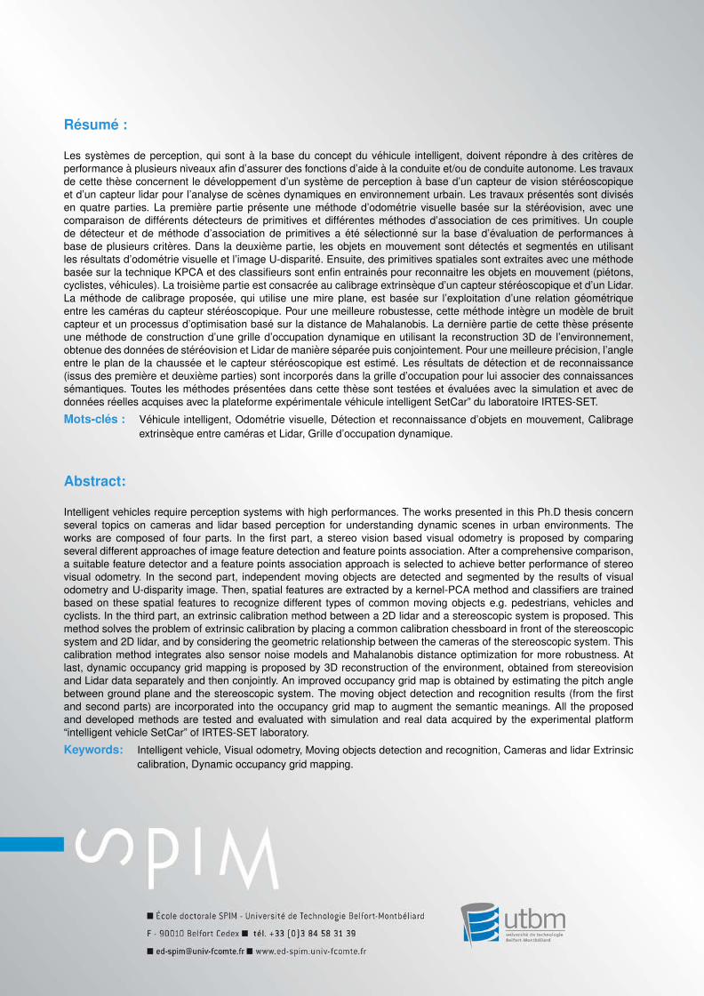
Resume :
Les systemes de perception, qui sont a la base du concept du vehicule intelligent, doivent repondre a des criteres de
performance a plusieurs niveaux afin d’assurer des fonctions d’aide a la conduite et/ou de conduite autonome. Les travaux
de cette these concernent le developpement d’un systeme de perception a base d’un capteur de vision stereoscopique
et d’un capteur lidar pour l’analyse de scenes dynamiques en environnement urbain. Les travaux presentes sont divises
en quatre parties. La premiere partie presente une methode d’odometrie visuelle basee sur la stereovision, avec une
comparaison de differents detecteurs de primitives et differentes methodes d’association de ces primitives. Un couple
de detecteur et de methode d’association de primitives a ete selectionne sur la base d’evaluation de performances a
base de plusieurs criteres. Dans la deuxieme partie, les objets en mouvement sont detectes et segmentes en utilisant
les resultats d’odometrie visuelle et l’image U-disparite. Ensuite, des primitives spatiales sont extraites avec une methode
basee sur la technique KPCA et des classifieurs sont enfin entraines pour reconnaitre les objets en mouvement (pietons,
cyclistes, vehicules). La troisieme partie est consacree au calibrage extrinseque d’un capteur stereoscopique et d’un Lidar.
La methode de calibrage proposee, qui utilise une mire plane, est basee sur l’exploitation d’une relation geometrique
entre les cameras du capteur stereoscopique. Pour une meilleure robustesse, cette methode integre un modele de bruit
capteur et un processus d’optimisation base sur la distance de Mahalanobis. La derniere partie de cette these presente
une methode de construction d’une grille d’occupation dynamique en utilisant la reconstruction 3D de l’environnement,
obtenue des donnees de stereovision et Lidar de maniere separee puis conjointement. Pour une meilleure precision, l’angle
entre le plan de la chaussee et le capteur stereoscopique est estime. Les resultats de detection et de reconnaissance
(issus des premiere et deuxieme parties) sont incorpores dans la grille d’occupation pour lui associer des connaissances
semantiques. Toutes les methodes presentees dans cette these sont testees et evaluees avec la simulation et avec de
donnees reelles acquises avec la plateforme experimentale vehicule intelligent SetCar” du laboratoire IRTES-SET.
Mots-cles : Vehicule intelligent, Odometrie visuelle, Detection et reconnaissance d’objets en mouvement, Calibrage
extrinseque entre cameras et Lidar, Grille d’occupation dynamique.
Abstract:
Intelligent vehicles require perception systems with high performances. The works presented in this Ph.D thesis concern
several topics on cameras and lidar based perception for understanding dynamic scenes in urban environments. The
works are composed of four parts. In the first part, a stereo vision based visual odometry is proposed by comparing
several different approaches of image feature detection and feature points association. After a comprehensive comparison,
a suitable feature detector and a feature points association approach is selected to achieve better performance of stereo
visual odometry. In the second part, independent moving objects are detected and segmented by the results of visual
odometry and U-disparity image. Then, spatial features are extracted by a kernel-PCA method and classifiers are trained
based on these spatial features to recognize different types of common moving objects e.g. pedestrians, vehicles and
cyclists. In the third part, an extrinsic calibration method between a 2D lidar and a stereoscopic system is proposed. This
method solves the problem of extrinsic calibration by placing a common calibration chessboard in front of the stereoscopic
system and 2D lidar, and by considering the geometric relationship between the cameras of the stereoscopic system. This
calibration method integrates also sensor noise models and Mahalanobis distance optimization for more robustness. At
last, dynamic occupancy grid mapping is proposed by 3D reconstruction of the environment, obtained from stereovision
and Lidar data separately and then conjointly. An improved occupancy grid map is obtained by estimating the pitch angle
between ground plane and the stereoscopic system. The moving object detection and recognition results (from the first
and second parts) are incorporated into the occupancy grid map to augment the semantic meanings. All the proposed
and developed methods are tested and evaluated with simulation and real data acquired by the experimental platform
“intelligent vehicle SetCar” of IRTES-SET laboratory.
Keywords: Intelligent vehicle, Visual odometry, Moving objects detection and recognition, Cameras and lidar Extrinsic
calibration, Dynamic occupancy grid mapping.