Making a Map-making Robot:Using the IKAROS System to Implement the Occupancy Grid Algorithm.

Rasmus Bååth, Birger JohanssonLund University Cognitive Science

Kungshuset, Lundagård, 222 22 Lundrasmus.baath@lucs.lu.se, birger.johansson@lucs.lu.se

Abstract

This paper describes an implementation of the occu-pancy grid algorithm, one of the most popular algo-rithms for robotic mapping. The algorithm is imple-mented on a robot setup at Lund University Cogni-tive Science (LUCS), and a number of experiments areconducted where the algorithm is exposed to differentkinds of noise. The outcome show that the algorithmperforms well given its parameters are tuned right.The conclusion is made that, in spite of its limita-tions, the occupancy grid map algorithm is a robustalgorithm that works well in practice.

1 Introduction

Maps are extremely useful artifacts. A map helps usrelate to places we have never been to and shows usthe way if we decide we want to go there. For an au-tonomous robot a map is even more useful as it could,if it is detailed enough, serve as the robot’s internalrepresentation of the world. The field of robotic map-ping is quite young and started to receive attentionfirst in the early 80s. Since then a lot of effort hasgone into constructing robust robotic mapping algo-rithms, but the challenge is great as the way a humanintuitively would build a map can not be directly ap-plicable to a robot. Whereas a human possesses supe-rior vision sensors and can locate herself by identify-ing landmarks, a robot, most often, only have sensorsthat approximates the distance to the closest walls.The conditions of robotic mapping actually closer re-sembles the conditions for a 15th century ship map-ping uncharted water. Similar to the ship the robotonly knows the approximate distance to the closestobstacles, it could happen that all obstacles are so faraway that the robot senses void and it is often difficultfor the robot to keep track of its position and heading.As opposed to the ship, a robot using a faulty mapwill bump into walls in a disgraceful manner, while

the ship, on the other hand, might discover America.A long-standing goal of AI and robotics research

has been to construct truly autonomous robot’s, ca-pable of reasoning about and interacting with theirenvironment. It is hard to see how this could be re-alized without general robust mapping algorithms.

1.1 The Approach of this PaperThis paper describes an implementation of a mapbuilding algorithm for a robot setup at LUCS. Themain characteristics of the robot setup are that theenvironment is static and that the pose is given, there-fore it does not induce all the difficulties mentionedabove. The given pose is not without noise but therewill never be the problem with cumulative positionnoise. Even if the problem is eased it is still far fromtrivial thus interesting in its own right. The setupwill be further described in section 2. Given theseprecondition the occupancy grid map algorithm, firstdescribed by Elfes and Moravec [3], was chosen. Theoccupancy grid map algorithm was implemented anda number of experiments were conducted to investi-gate how it would perform given different types ofsensor noise. The results of the experiments are pre-sented in section 3.2.

1.2 The Occupancy Grid Map Algo-rithm

The occupancy grid map algorithm was developed inthe mid 80s by Efes and Moravec and is a recursiveBayesian estimation algorithm. Here recursive meansthat in order integrate an nth sensor reading into amap no history of sensor readings is necessary. This isa useful property which implies that sensor readingscan be integrated online and that the space and timecomplexity is constant with respect to the number ofsensor readings. The algorithm is Bayesian becausethe central update equation is based on Bayes theo-rem:

P (A|B) =P (B|A)P (A)

P (B)

which answers the question “what is the proba-bility of A given B”, if we know the probabilitiesP (B|A), P (A) and P (B).

The map data structure is a grid, in 2D or 3D, thatrepresents a region in space. This paper will treatthe 2D case, thus the region is a rectangle. The valueof each cell of the grid is the estimated probabilitythat the corresponding area in space is occupied. Theregion corresponding to a cell is always consideredcompletely occupied or completely empty. One canhave different definitions regarding whether a regionis free or occupied, but often a region is consideredoccupied if any part of it is occupied.

The algorithm consists of two separate parts: theupdate equation and a sensor model. The updateequation is the basis of the algorithm and does nothave to change for different robot setups. The sensormodel on the other hand depends on the robot setupand each robot setup requires a customized sensormodel. One can construct sensor models in manyways but the basic approach is described in section1.3.

The computational complexity of the algorithm de-pends on the implementation of the sensor model.Apart from that, each update loop have time com-plexity O(n′m′), where n′ and m′ are the numberof columns and rows of the grid that are affectedby the current sensor reading. The space complex-ity is O(nm) where n and m are the total numberof columns and rows of the grid. An accessible in-troduction to occupancy grid maps is given by Elfes[2].

The original algorithm is limited in several ways. Itrequires that the robot’s pose is given, thus it can notrely solely on the odometry of the robot. It presumesa static environment or requires sensor readings wheredynamic obstacles have been filtered. Finally the areato be mapped has to be specified in advance. Thismight sound like severe limitations but in many robotsetups one can assume a static environment and thatthere is a way to deduce the robot’s pose. The originalalgorithm has also been successfully extended to dealwith e.g. unknown robot poses [7].

1.3 The Inverse Sensor Model

A sensor model is a procedure for calculating theprobability P (st|m, pt), that is the probability to getsensor reading st given map m and pose pt at time t.Therefore it follows that the procedure for calculatingP (m|st, pt) is called an inverse sensor model, that is

the probability of m given only one sensor reading.An inverse sensor model can be though of as func-tion ism(st, pt) that returns a grid the size of g wherethe probabilities of P (m|st,pt) are imprinted. Thereis not only one correct way to construct ism(st, pt)for a given sensor, different approaches have differentadvantages.

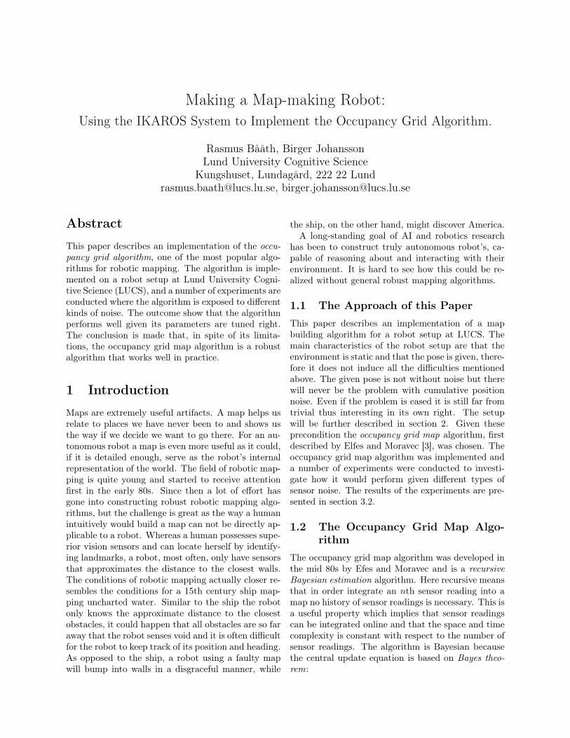
An example of how the output of an inverse sensormodel could look is given in figure 1.

Figure 1: Illustration of an inverse sensor model for arobot equipped with infra-red proximity sensors.

The picture to the left show what the robot senses.The picture to the right is the resulting occupationalprobabilities. White denotes occupied space,black de-notes free space and gray denotes unknown space. No-tice how the black strokes fade with the distance tothe robot. This indicates that the probability that asensor detects an obstacle decreases with the distanceto the obstacle.

An inverse sensor model can be built by hand orlearned, for an example of the first see Elfes andMoravec [3] or the one described in section 2.1.5, foran example of the latter see Thrun et al. [6].

2 ImplementationIn order to understand the design choices made a de-scription of the robot setup will first be given, thenthe implementation will be described. The setup iscurrently used in the ongoing research regarding robotattention and one purpose of the implementation wasthat it should be possible to use in this context.

2.1 The Robot SetupThe robot used is the e-puck, a small, muffin sizedrobot developed by École Polytechnique Fédérale deLausanne (www.e-puck.org). Its a differential wheeledrobot boosting eight infra-red proximity sensors, acamera, accelerometer and Bluetooth connectivity.The e-puck also have very precise step motors to con-trol its wheels. One problem is that no matter how

precise the e-pucks odometry is it can not solely beused to determine the robot’s poses. Another prob-lem is the proximity sensors of the e-puck. They havevery limited range, roughly 10 cm, and are sensitivewith respect to light conditions.

In order to remedy these problems a video camerahas been placed in the ceiling of room where the robotexperiments take place. The robots movements arerestricted to a 2× 2 m2 “sandbox” and objects in thisarea have been given color codes. Robots are wearingbright red plastic cups, the floor, the free space, isdark gray and obstacles are white. Images from thecamera are processed in order to extract the poses ofthe robots and an image where only the obstacles arevisible. Given this image and a robot’s pose a circlesector is cut out of the image, its center being therobot’s position and its direction being the robot’sheading. By using this as the robot’s sensor readingthe robot can be treated as if it had a high resolu-tion proximity sensor. The robots are controlled overBluetooth link.

2.1.1 Ikaros

The whole system is implemented using Ikaros, amulti-purpose framework developed at LUCS. Ikarosis written in C++ and is intended for, among otherthings, brain modeling and robot control. The cen-tral concept in Ikaros is the module, and a systembuilt in Ikaros is a collection of connected module’s.An Ikaros module is simply put, a collection of in-puts and an algorithm that works on these, the resultending up in a number of outputs. A module’s in-puts and outputs are defined by an Ikaros control fileusing an XML based language while the algorithm isimplemented in C++.

A module’s outputs can be connected to other mod-ule’s inputs and to build a working system in Ikarosyou would specify these connection in a control file. Inthis control file you could also give arguments to the

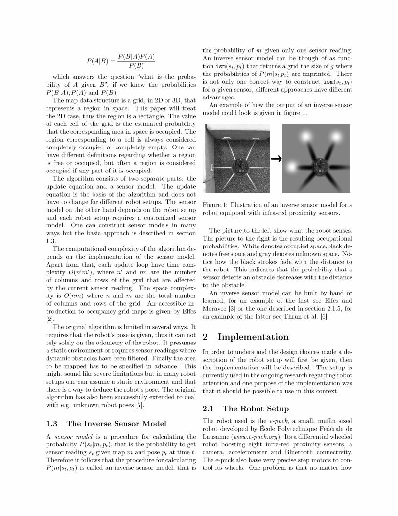
Figure 2: The e-puck.

modules. The data that can be transmitted betweenmodules can only be in one format, that is arrays andmatrices of floats. An Ikaros system works in discretetime-steps, so called “ticks”. Each tick every modulereceives input and produces output.

Ikaros comes with a number of modules, both sim-ple utility modules and more advanced such as sev-eral image feature extraction modules. Ikaros alsoincludes a web interface that can display outputs indifferent ways. For a detailed introduction to Ikarossee Balkenius et al. [1].

2.1.2 Overview of the System

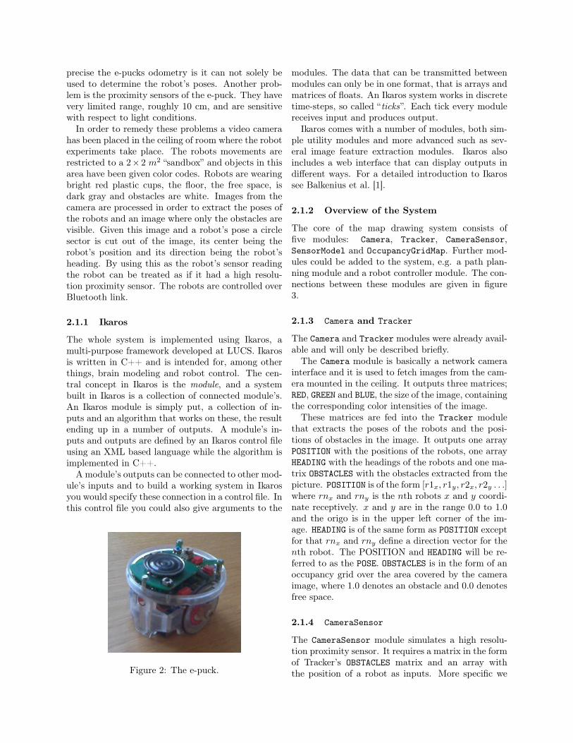
The core of the map drawing system consists offive modules: Camera, Tracker, CameraSensor,SensorModel and OccupancyGridMap. Further mod-ules could be added to the system, e.g. a path plan-ning module and a robot controller module. The con-nections between these modules are given in figure3.

2.1.3 Camera and Tracker

The Camera and Tracker modules were already avail-able and will only be described briefly.

The Camera module is basically a network camerainterface and it is used to fetch images from the cam-era mounted in the ceiling. It outputs three matrices;RED, GREEN and BLUE, the size of the image, containingthe corresponding color intensities of the image.

These matrices are fed into the Tracker modulethat extracts the poses of the robots and the posi-tions of obstacles in the image. It outputs one arrayPOSITION with the positions of the robots, one arrayHEADING with the headings of the robots and one ma-trix OBSTACLES with the obstacles extracted from thepicture. POSITION is of the form [r1x, r1y, r2x, r2y . . .]where rnx and rny is the nth robots x and y coordi-nate receptively. x and y are in the range 0.0 to 1.0and the origo is in the upper left corner of the im-age. HEADING is of the same form as POSITION exceptfor that rnx and rny define a direction vector for thenth robot. The POSITION and HEADING will be re-ferred to as the POSE. OBSTACLES is in the form of anoccupancy grid over the area covered by the cameraimage, where 1.0 denotes an obstacle and 0.0 denotesfree space.

2.1.4 CameraSensor

The CameraSensor module simulates a high resolu-tion proximity sensor. It requires a matrix in the formof Tracker’s OBSTACLES matrix and an array withthe position of a robot as inputs. More specific we

Figure 3: The connections between the modules of the map drawing system, with added path planning androbot control modules.

want to simulate a top mounted stereo camera. TheCameraSensor module takes arguments specifying herange of the camera and the breadth of the view.Given the pose of the robot a square is cut out ofthe matrix, this square is rotated and projected ontoanother matrix representing the SENSOR READING ofthe robot. The SENSOR READING shows everything inthe cut out square, even obstacles behind walls. Somesimple ray-casting will solve this. Rays are shot fromthe center of the robot to the edge lying on the op-posite side of the SENSOR READING matrix so that thecells touched by the rays form a circle sector. If aray hits an obstacle the ray stops and all cells nottouched by any ray obtains the value 0.5 indicatingit’s not part of the sensor reading. CameraSensorthen outputs SENSOR READING.

2.1.5 CameraSensorModel

The CameraSensorModel is an inverse sensormodel tailored to work with the output of theCameraSensor. CameraSensorModel has two out-puts, both required by OccupancyGridMap: AFFECTEDGRID REGION and OCC PROB GRID. OCC PROB GRID isa matrix the same size as the final occupancy gridthat contains the probabilities P (m|st, pt). AFFECTEDGRID REGION is an array of length four defining a boxbounding the area of the occupancy grid that is af-fected by the OCC PROB GRID. The rationale behindthis is that OccupancyGridMap should not have to up-date the whole occupancy grid when only a small areaof it is affected by the current SENSOR READING.

The SENSOR READING from CameraSensor is al-ready in the format of an occupancy grid, so trans-forming this into OCC PROB GRID in the formatthe OccupancyGridMap module requires, is prettystraight forward. First OCC PROB GRID is initializedwith P (m), the prior probability, given as an ar-gument to CameraSensorModel. Then the SENSOR

READING is rotated and translated, according to therobot’s pose, so that it covers the correspondingarea of the OCC PROB GRID. The SENSOR READING isthen imprinted on the OCC PROB GRID. The valuesof SENSOR READING; 1.0, 0.5 and 0.0, should not beused directly as they do not correspond to the rightprobabilities. Instead 0.5 is substituted by the priorprobability and 1.0 and 0.0 are substituted by two val-ues free_prob and occ_prob given as arguments toCameraSensorModel. The values of free_prob andocc_prob should reflect probability that the informa-tion in SENSOR READING is correct. As the Cameraand Tracker modules are quite exact good valuesseems to be; free_prob= 0.05 and occ_prob = 0.95.The performance of occupancy grid algorithm de-pends heavily on these values and they have to be ad-justed according to the reliability of SENSOR READING.This will be further discussed in section 3.2.

2.1.6 OccupancyGridMap

The OccupancyGridMap take two inputs in the for-mats of OCC PROB GRID and AFFECTED GRID REGION.OccupancyGridMap also contains the state of the oc-cupancy grid constructed so far; MAP GRID, and theprior probability; pri_prob, given as an argument.The MAP GRID is initialized by giving each cell thevalue of pri_prob.

The purpose of OccupancyGridMap is to updateMAP GRID using the update equation of the occupancygrid map algorithm. This is done by applying this onall cells in MAP GRID that are inside the box definedby AFFECTED GRID REGION. Here follows the updateequation taken directly from the code:

for(int i = affected_grid_region[2];i <= affected_grid_region[3]; i++){

for(int j = affected_grid_region[0];j <= affected_grid_region[1]; j++){

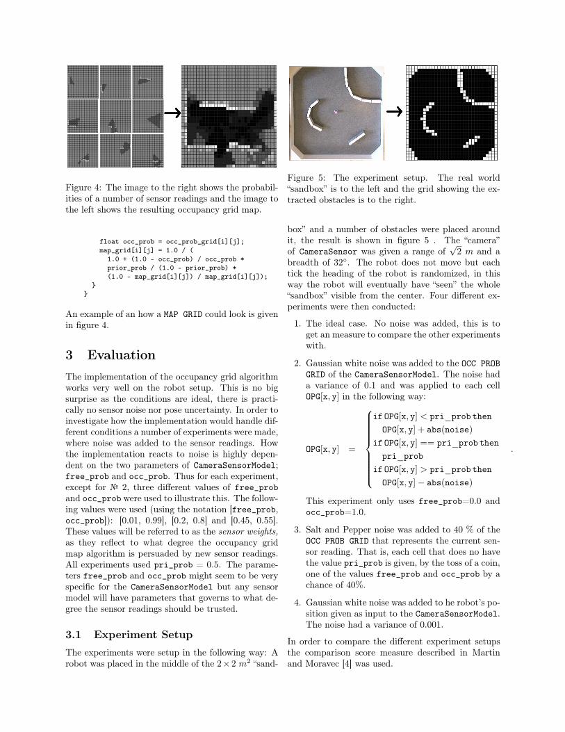
Figure 4: The image to the right shows the probabil-ities of a number of sensor readings and the image tothe left shows the resulting occupancy grid map.

float occ_prob = occ_prob_grid[i][j];map_grid[i][j] = 1.0 / (

1.0 + (1.0 - occ_prob) / occ_prob *prior_prob / (1.0 - prior_prob) *(1.0 - map_grid[i][j]) / map_grid[i][j]);

}}

An example of an how a MAP GRID could look is givenin figure 4.

3 Evaluation

The implementation of the occupancy grid algorithmworks very well on the robot setup. This is no bigsurprise as the conditions are ideal, there is practi-cally no sensor noise nor pose uncertainty. In order toinvestigate how the implementation would handle dif-ferent conditions a number of experiments were made,where noise was added to the sensor readings. Howthe implementation reacts to noise is highly depen-dent on the two parameters of CameraSensorModel;free_prob and occ_prob. Thus for each experiment,except for № 2, three different values of free_proband occ_prob were used to illustrate this. The follow-ing values were used (using the notation [free_prob,occ_prob]): [0.01, 0.99], [0.2, 0.8] and [0.45, 0.55].These values will be referred to as the sensor weights,as they reflect to what degree the occupancy gridmap algorithm is persuaded by new sensor readings.All experiments used pri_prob = 0.5. The parame-ters free_prob and occ_prob might seem to be veryspecific for the CameraSensorModel but any sensormodel will have parameters that governs to what de-gree the sensor readings should be trusted.

3.1 Experiment Setup

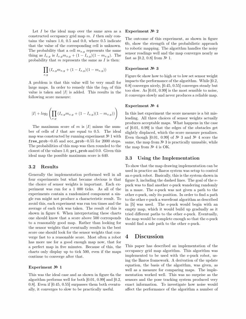
The experiments were setup in the following way: Arobot was placed in the middle of the 2×2 m2 “sand-

Figure 5: The experiment setup. The real world“sandbox” is to the left and the grid showing the ex-tracted obstacles is to the right.

box” and a number of obstacles were placed aroundit, the result is shown in figure 5 . The “camera”of CameraSensor was given a range of

√2 m and a

breadth of 32◦. The robot does not move but eachtick the heading of the robot is randomized, in thisway the robot will eventually have “seen” the whole“sandbox” visible from the center. Four different ex-periments were then conducted:

1. The ideal case. No noise was added, this is toget an measure to compare the other experimentswith.

2. Gaussian white noise was added to the OCC PROBGRID of the CameraSensorModel. The noise hada variance of 0.1 and was applied to each cellOPG[x, y] in the following way:

OPG[x, y] =

if OPG[x, y] < pri_prob thenOPG[x, y] + abs(noise)

if OPG[x, y] == pri_prob thenpri_prob

if OPG[x, y] > pri_prob thenOPG[x, y]− abs(noise)

.

This experiment only uses free_prob=0.0 andocc_prob=1.0.

3. Salt and Pepper noise was added to 40 % of theOCC PROB GRID that represents the current sen-sor reading. That is, each cell that does no havethe value pri_prob is given, by the toss of a coin,one of the values free_prob and occ_prob by achance of 40%.

4. Gaussian white noise was added to he robot’s po-sition given as input to the CameraSensorModel.The noise had a variance of 0.001.

In order to compare the different experiment setupsthe comparison score measure described in Martinand Moravec [4] was used.

Let I be the ideal map over the same area as aconstructed occupancy grid map m. I then only con-tains the values 1.0, 0.5 and 0.0, where 0.5 indicatethat the value of the corresponding cell is unknown.The probability that a cell mx,y represents the samething as Ix,y is Ix,ymx,y + (1 − Ix,y)(1 −mx,y). Theprobability that m represents the same as I is then:∏

x,y

(Ix,ymx,y + (1− Ix,y)(1−mx,y))

A problem is that this value will be very small forlarge maps. In order to remedy this the log2 of thisvalue is taken and |I| is added. This results in thefollowing score measure:

|I|+ log2

(∏x,y

(Ix,ymx,y + (1− Ix,y)(1−mx,y))

)

The maximum score of m is |I| minus the num-ber of cells of I that are equal to 0.5. The idealmap was constructed by running experiment № 1 withfree_prob=0.45 and occ_prob=0.55 for 2000 steps.The probabilities of this map was then rounded to theclosest of the values 1.0, pri_prob and 0.0. Given thisideal map the possible maximum score is 640.

3.2 Results

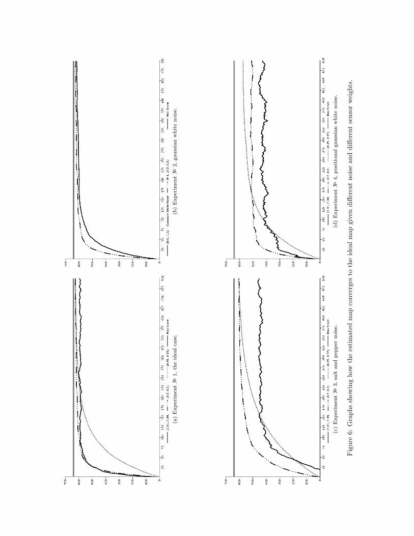
Generally the implementation performed well in allfour experiments but what became obvious is thatthe choice of sensor weights is important. Each ex-periment was run for a 1 000 ticks. As all of theexperiments contain a randomized component a sin-gle run might not produce a characteristic result. Toavoid this, each experiment was run ten times and theaverage of each tick was taken. The result of this isshown in figure 6. When interpretating these chartsone should know that a score above 500 correspondsto a reasonably good map. Rather than looking forthe sensor weights that eventually results in the bestscore one should look for the sensor weights that con-verge fast to a reasonable score. Most often a robothas more use for a good enough map now, that fora perfect map in five minutes. Because of this, thecharts only display up to tick 500, even if the mapscontinue to converge after that.

Experiment № 1

This was the ideal case and as shown in figure 6a thealgorithm performs well for both [0.01, 0.99] and [0.2,0.8]. Even if [0.45, 0.55] surpasses them both eventu-ally, it converges to slow to be practically useful.

Experiment № 2

The outcome of this experiment, as shown in figure6b, show the strength of the probabilistic approachto robotic mapping. The algorithm handles the noisysensor readings well and the map converges nearly asfast as [0.2, 0.8] from № 1.

Experiment № 3

Figure 6c show how to high or to low set sensor weightimpacts the performance of the algorithm. While [0.2,0.8] converges nicely, [0.45, 0.55] converges steady buttoo slow. As [0.01, 0.99] is the most sensible to noise,it converges slowly and never produces a reliable map.

Experiment № 4

In this last experiment the score measure is a bit mis-leading. All three choices of sensor weights actuallyproduces acceptable maps. What happens in the caseof [0.01, 0.99] is that the edges of the obstacles getslightly displaced, which the score measure penalizes.Even though [0.01, 0.99] of № 3 and № 4 score thesame, the map from № 3 is practically unusable, whilethe map from № 4 is OK.

3.3 Using the ImplementationTo show that the map drawing implementation can beused in practice an Ikaros system was setup to controlan e-puck robot. Basically, this is the system shown infigure 3, including the dashed lines. The goal of the e-puck was to find another e-puck wandering randomlyin a maze. The e-puck was not given a path to theother e-puck, only its position. In order to find a pathto the other e-puck a wavefront algorithm as describedin [5] was used. The e-puck would begin with anempty map, which it would build up gradually as ittried different paths to the other e-puck. Eventually,the map would be complete enough so that the e-puckwould find a safe path to the other e-puck.

4 DiscussionThis paper has described an implementation of theoccupancy grid map algorithm. This algorithm wasimplemented to be used with the e-puck robot, us-ing the Ikaros framework. A derivation of the updateequation, the basis of the algorithm, was given, aswell as a measure for comparing maps. The imple-mentation worked well. This was no surprise as thesensors and the pose tracking system produced veryexact information. To investigate how noise wouldaffect the performance of the algorithm a number of

(a)

Exp

erim

ent

№1,

the

idea

lca

se.

(b)

Exp

erim

ent

№2,

gaus

sian

whi

teno

ise.

(c)

Exp

erim

ent

№3,

salt

and

pepp

erno

ise.

(d)

Exp

erim

ent

№4,

posi

tion

alga

ussi

anw

hite

nois

e.

Figure6:

Graph

sshow

ingho

wtheestimated

map

conv

ergesto

theidealm

apgivendiffe

rent

noisean

ddiffe

rent

sensor

weigh

ts.

experiments were conducted. Gaussian white noisewas applied to the sensors and the pose tracking sys-tem, and so called salt and pepper noise was appliedto the sensors only. To show that the implementationwas usable in practice a system was constructed thatmade an e-puck draw an occupancy grid map. Thee-puck then used this map to find a path to anothere-puck wandering randomly.

4.1 Evaluation of the Experiments

Experiment № 1 show that the algorithm works wellgiven ideal preconditions. This is no surprise, but itis important note how the tuning of sensor weightsimpacts the performance. When the sensor weightsare set so that the algorithm put little trust in thesensors, the map converges steadily but unnecessarilyslow.

Experiment № 2 and 3 show the strength of the al-gorithm, its capability to handle independent noise.Both the sensor readings of № 2 and 3 are very noisy,indeed it is often hard for the human eye to separatetrue obstacles from noise. The algorithm managesthis well, given that the sensor weights are set so thatthe algorithm does not put to much trust in the sen-sors.

Experiment № 4 show that the algorithm can pro-duce an acceptable map when the position is noisy.The tuning of the sensor weights does not have suchan impact as figure 6d might suggest. This is dueto the fact that the score measure does not rewardcorrectly identified obstacles that are off by a smalldistance. One problem with positional noise is thatit does not lead to sensor noise that is statisticallyindependent. If the positional noise is to large thealgorithm will not be able to handle it no matter howthe sensor weights are tuned.

The implementation of the e-puck control systemdescribed in section 3.3 worked well in simulation.The two robots steadily moved towards each other,drawing the map and avoiding obstacles as they wentalong. When trying this with the real robots therewere some problems. The Trackermodule sometimesconfused one of the robots for the other one. Alsothere were some problems communicating with tworobots over one Bluetooth connection. Nevertheless,the occupancy grid map algorithm, in combinationwith the wavefront path planner, always produced acorrect path, even if the robot had troubles followingit.

4.2 ConclusionIn spite of its limitation the occupancy grid map al-gorithm is, as this paper has shown, a robust andversatile algorithm. When in need for a robotic map-ping algorithm one should have good reasons not toconsider using it.

References[1] C. Balkenius, J. Morén, B. Johansson, and

M. Johnsson. Ikaros: Building cognitive modelsfor robots. Advanced Engineering Informatics, 24(1):40–48, 2009.

[2] A. Elfes. Using occupancy grids for mobile robotperception and navigation. Computer, 22(6):46–57, June 1989. ISSN 0018-9162.

[3] A. Elfes and H. Moravec. High resolution mapsfron wide angle sonar. IEEE International confer-ence on Robotics and Automation, 1985.

[4] Martin C. Martin and Hans Moravec. Robot ev-idence grids. Technical Report CMU-RI-TR-96-06, Robotics Institute, Carnegie Mellon Univer-sity, Pittsburgh, PA, March 1996.

[5] S. Russell and P. Norvig. Artificial Intelligence -a Modern Approach, 2nd edition. Prentice Hall,2002.

[6] S. Thrun, A. Bücken, W. Burgard, D. Fox,T. Fröhlinghaus, D. Henning, T. Hofmann,M. Krell, and T. Schmidt. Map learning and high-speed navigation in RHINO. In D. Kortenkamp,R.P. Bonasso, and R Murphy, editors, AI-basedMobile Robots: Case Studies of Successful RobotSystems. MIT Press, 1998.

[7] S. Thrun, M. Bennewitz, W. Burgard, A.B. Cre-mers, F. Dellaert, D. Fox, D. Hähnel, C. Rosen-berg, N. Roy, J. Schulte, and D. Schulz. MIN-ERVA: A second generation mobile tour-guiderobot. In Proceedings of the IEEE InternationalConference on Robotics and Automation (ICRA),1999.