HAL Id: hal-01576974https://hal.archives-ouvertes.fr/hal-01576974

Submitted on 24 Aug 2017

HAL is a multi-disciplinary open accessarchive for the deposit and dissemination of sci-entific research documents, whether they are pub-lished or not. The documents may come fromteaching and research institutions in France orabroad, or from public or private research centers.

L’archive ouverte pluridisciplinaire HAL, estdestinée au dépôt et à la diffusion de documentsscientifiques de niveau recherche, publiés ou non,émanant des établissements d’enseignement et derecherche français ou étrangers, des laboratoirespublics ou privés.

Using Evidential Occupancy Grid for Vehicle TrajectoryPlanning Under Uncertainty with Tentacles

Hafida Mouhagir, Véronique Cherfaoui, Reine Talj, François Aioun, FranckGuillemard

To cite this version:Hafida Mouhagir, Véronique Cherfaoui, Reine Talj, François Aioun, Franck Guillemard. Using Evi-dential Occupancy Grid for Vehicle Trajectory Planning Under Uncertainty with Tentacles. 20th IEEEInternational Conference on Intelligent Transportation Systems (ITSC 2017), Oct 2017, Yokohama,Japan. pp.1-7. �hal-01576974�

Using Evidential Occupancy Grid for Vehicle Trajectory Planning Under

Uncertainty with TentaclesHafida Mouhagir1,2, Véronique Cherfaoui1 , Reine Talj 1, François Aioun2, Franck Guillemard2

Abstract—The uncertainty in environment perception is oneof the challenges that we face in trajectory planning. Forautonomous vehicle to be efficient, they need to be able to dealwith this kind of uncertainty. In this work, we combine twoexisting frameworks: the Belief Functions to build evidentialoccupancy grid and clothoid tentacles for trajectory planning.First, we use evidential grids to represent the environment andthe uncertainties which arise from ignorance and errors duringthe perception process. Secondly, we generate a set of clothoidtentacles in the egocentered reference frame related to theego-vehicle, those tentacles represent possible local trajectories.Thirdly, we modify the evidential grid in order to take intoconsideration some traffic rules such as safety distance betweenvehicles. Then to choose the best tentacle to execute, we usereward system of a Markov Decision Process-like model toevaluate generated tentacles regarding several criteria includinguncertainty represented by the evidential grid. Real and simu-lated data were used to validate the planning algorithm withevidential grids.

I. INTRODUCTION

Autonomous driving requires decision making in dynamicand uncertain environments. The uncertainties come from:imperfect knowledge of the vehicle model noisy sensor data,occlusions in the perception system, and poor predictabilitydue to the inability of measuring other driver’s intentions.

To solve environment predictability, Partially ObservableMarkov Decision Process (POMDP) [8] is a method whichallows to find an optimal action given the uncertainty of theperception system and/or future behavior. It provides nearoptimum solutions for decision making with a variable numberof traffic participants and with unknown maneuver intentions.This approach expects that the ego-vehicle will continuouslygather information about its surrounding and incorporatesthem in the decision making.

Brechtel et al. [3] use Continuous POMDP in decisionmaking to address both problems of noisy sensor measurementand the environment occlusion in intersection scenarios. Theauthors of [19] presented a QMDP-based approach (QMDPis a hybrid between MDP and POMDP, this algorithm gen-eralizes the MDP-optimal value function defined over states,into a POMDP-style value functions over beliefs) for single-lane behaviors. They show that considering uncertainty in thebehavior of the leading vehicle as well as limitations of theperception improves robustness. However, they used a statespace that is tailored for single-lane driving.

The authors are with 1Sorbonne universités, Université de Technologiede Compiègne (UTC), CNRS Heudiasyc UMR 7253, 2PSA Groupe,Direction scientifique, Centre technique de Vélizy, France. E-mail: {hafida.mouhagir, reine.talj, veronique.cherfaoui}@hds.utc.fr,{franck.guillemard, françois.aioun}@mpsa.com

In this work, we focus on the grid-based approach tomodel the environment, including the obstacle information.The reason behind this choice instead of object level approachfor example is that we are looking to have a planning methodthat works with as few sensors as possible.

The occupancy grids are constructed by interpreting thesensor information into the grid cell values. When interpret-ing the sensor data into occupancy information, uncertaintyinevitably arises from ignorance and errors. Ignorance isdue to the perception of new areas or to occlusions anderrors come from noisy measurements and imprecise poseestimation. In the literature, the Bayesian framework is themost popular method to tackle this problem by representingthe uncertainties by means of probability, then the update stepadopts the Bayesian Theorem to fuse new information. In [5],the authors present a method to estimate the probability ofcollision with uncertainty in position, shape and velocity of theobstacles. They used Bayesian Occupancy Filter (BOF) witchis a dynamic occupancy grid where an estimation of velocityis stored as well as the probability of occupation. However,occlusions and free space have the same low probability ofoccupation. This problem can be solved using the theory ofbelief function.

First introduced by [4] and formalized by [16], the frame-work of belief function has a growing number of applicationsin artificial intelligence, information fusion, classification, re-liability and risk analysis, etc. In [13], the authors used thisframework to build evidential occupancy grid that provides theego-vehicle with additional information about its environment.They detect moving objects by analyzing conflicting informa-tion.

In this work, we use evidential grids elaborated thanksto a lidar range scanner to model the uncertainties of theenvironment. Once the information on the surrounding envi-ronment is provided by the grid, the next step is to interpretthis information to plan a trajectory using clothoid tentacles.This trajectory planning approach [7] considers the currentdynamical state of the vehicle and makes a smooth variationsin the vehicle dynamic variables.

The contribution presented in this paper is the combinationof two existing frameworks: The Belief Functions to buildoccupancy grid and clothoid tentacles for trajectory planning.We modify the evidential grids to take into account the safetydistances between the ego-vehicle and obstacles. To choose thebest tentacle to execute, we use reward system of a MarkovDecision Process-like model to evaluate generated tentaclesregarding several criteria including uncertainty represented bythe evidential grid. Real and simulated data were used tovalidate the approach.

In Section II, we present the construction of the evidentialgrids for trajectory planning. In Section III, the trajectoryplanning algorithm and the reward system of the MDP likemodel are explained. First results based on real and simulateddata are discussed in Section IV followed by a conclusion ofthe paper including an outlook.

II. EVIDENTIAL OCCUPANCY GRID

The occupancy grids are used as an environment model, ifthe grid cells are filled with obstacle information in the formof evidence (mass or belief values for instance II-A), we callthis kind of grids “Evidential occupancy grids”.

A. Evidential frameworkThe theory of belief functions, also known as Demp-

ster–Shafer theory (DST), was proposed by Dempster [4], anddeveloped, among others, by Shafer [16] and Smets [18].

Let w be an unknown quantity with possible values in afinite domain ⌦ , called the frame of discernment. A piece ofevidence about w may be represented by a mass function mon ⌦ , defined as a function 2⌦ ! [0, 1] , such that m(;) = 0and

PA✓⌦ m(A) = 1 .

In the theory of Dempster-Shafer, a frame of discernment⌦ is defined to model a specific problem. In the occupancygrid framework, the frame of discernment is defined as: ⌦ ={F, O}, referred as the states (free or occupied) of each cell.The power set is defined as 2|⌦| = {;, F, O, ⌦}, with | ⌦ |is the cardinality of the set.

For quantitatively supporting the cell states, a mass function(also referred as Basic Belief Assignment BBA) is calculatedand provides four beliefs [m(;)m(F )m(O)m(⌦)] , wherem(A) represents respectively the quantity of evidence that thespace is Conflict , Free , Occupied , and Unknown .

Combination rulesThere is a large panel of combination rules to fuse BBAs (or

beliefs or mass functions) coming from independent sources.Usually, the BBAs should be defined in the same frame ofdiscernment. We describe the two most used ones in datafusion:

• The conjunctive rule proposed by Smets, is used tocombine two BBAs provided by reliable and distinctinformation sources [17]. The resulting BBA, denotedm1\2 , is defined by:

m1\2(A) =X

B\C=A

m1(B)m2(C) , 8A ✓ ⌦ (1)

The mass assigned to the empty set m1\2(;) quantifiesthe degree of disagreement between the two combinedsources.

• The Dempster rule, based on the orthogonal sum, is anormalized version of the conjunctive rule where the massof the empty set (mass on conflict) must be reallocatedover all focal elements in the case where m1\2(;) 6= 0thanks to a normalization factor, denoted K [16]. Thisrule, assuming pieces of evidence combined to be reliableand distinct, is defined as follows:

m1�2(A) = Km1\2(A) , 8A ✓ ⌦ (2)

and m1 �m2(;) = 0 where K = (1�m1\2(;))�1

B. Evidential occupancy gridIn this section, we present the perception grids used in our

approach. The construction of these grids is based on datacoming from a range sensor that provides information aboutthe occupancy/free of the cells.

The first step as described in [12], consists on computingthe PerceptionGrid from successive Lidar scans. For everysensor measurement, a ScanGrid is built with sensor modelthat translates the sensor information into an ego-centered grid.The BBA assignment respects the least commitment principle:the cells containing a Lidar point are occupied, the cellsbetween the sensor and the occupied cells are free and theother are unknown . The value of masses depends of theresolution of the grids and sensor performances.

The successive ScanGrids are fused in a unique resultingPerceptionGrid . To combine the new ScanGrid with thecurrent PerceptionGrid , two operations are carried out: first,a transformation (rotation and translation) computed with thevehicle displacement is applied to the ScanGrid, and thenall masses of the PerceptionGrid are discounted to give lessimportance to the past (Fig. 1). The fusion rule is based onthe conjunctive rule that can provide conflicting mass giveninformation about moving cells.

After PerceptionGrid processing, each cell has a massfunction with four beliefs on the state of the cell[m(;)m(F )m(O)m(⌦)] . Let consider a concrete case to il-lustrate these concepts, [m(;)m(F )m(O)m(⌦)]=[0 0 0.7 0.3]indicates an Occupied cell with 0.7 as a belief, the rest of themass is in Unknown . [m(;)m(F )m(O)m(⌦)]= [0 0.6 0 0.4]shows we have belief 0.6 in Free state, the rest of mass is inUnknown .

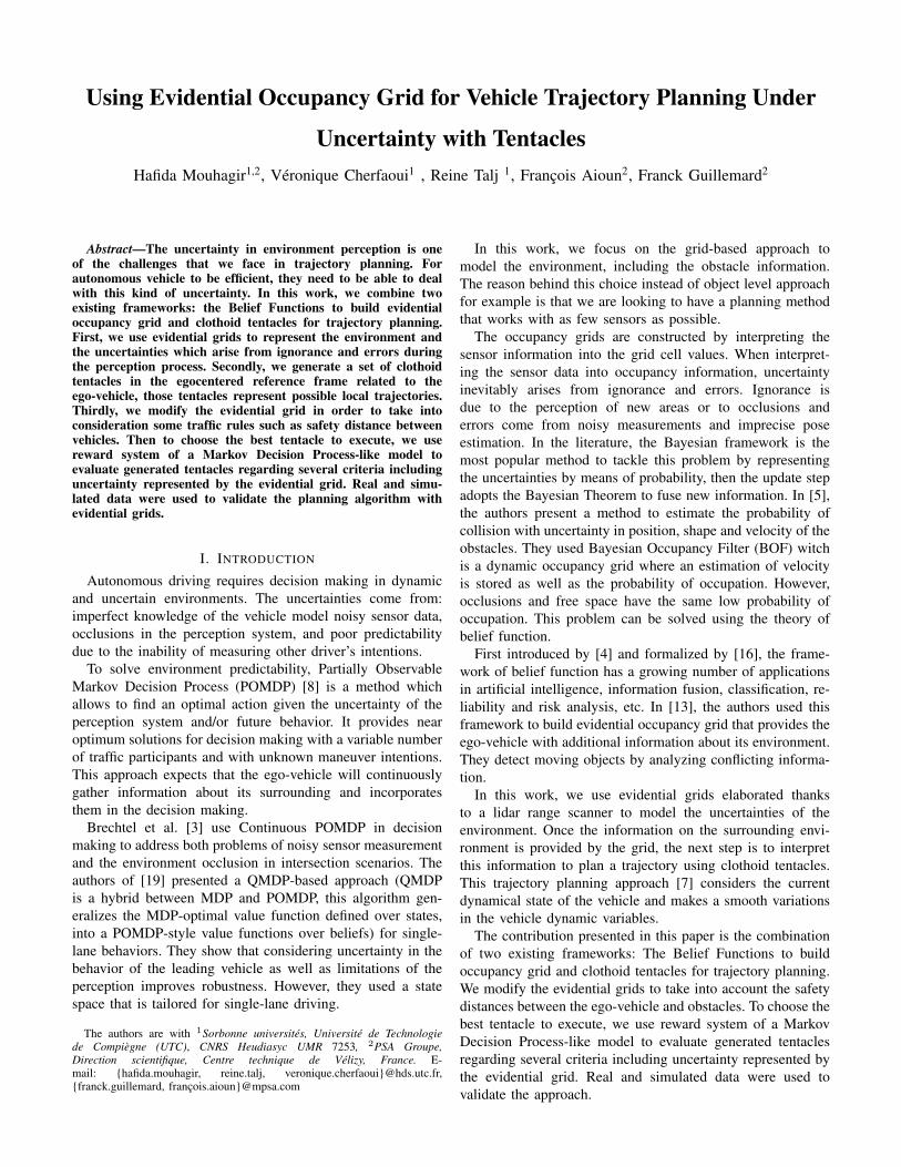
Figure 1: Example of an occupancy grid with its correspondingscene. The yellow triangle represents the position of the Lidar

sensor, the green color in the occupancy grid shows the free space, thered shows the occupied space, while the blue represents conflictingcells (before normalization) and the black represents unexplored cells.The color intensity reflects the certainty degree.

Once the perception grid is created, we add both themap information with road limits witch make it possible todistinguish between free navigable or non navigable space anddynamic obstacles velocity obtained using car-to-car commu-nication. With this new integrated information a new grid isobtained.

C. Evidential planning gridThe evidential occupancy grids provide information about

the occupation of the environment, this information are used toplan a trajectory to avoid collisions. However, the autonomousvehicles must be capable of avoiding collision, lane keepingand carrying out an overtaking maneuver while keeping safetydistances. Therefore, we propose to modify the grid by addinginformation about the edges of the road and by expanding thedynamic obstacles to include safety distances. The resultinggrid is what we call PlanGrid for planning grid.

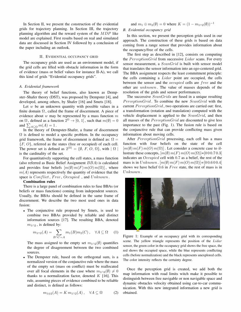
In Fig. 2- b), an example of enhancement of the mapwith road limit is given. The position of the vehicle and theinformation of the map was used to add a simple mask tothe evidential grid which integrates the edges of the roadby modifying the BBA of the cells out of the road surface.More elaborated methods of road segmentation exist. In theliterature, the authors of [2] propose a learning method forroad scene segmentation from a single image; the authors of[20] use Lidar as a sensor and prior maps and accurate poseestimation.

(a) (b) (c)

Figure 2: The PlanGrid (b) represents PerceptionGrid (a)

with the road’s edges information. The PlanGrid (c) presents alongitudinal obstacle widening.

In order to respect safety distances, the last step for build-ing the PlanGrid is the longitudinal expansion of dynamicobstacles in the occupancy grid (Fig. 2- c and Fig. 3). Wepropose to extend our previous work on the safety distance inbinary grids [14] considering both : the uncertainties modeledby mass function and the safety distance S

safe

calculated withformula proposed by [1]:

Ssafe

(vp

, vf

, amax

, �) =1

2amax

(v2f

� v2p

) + vf

� (3)

where vf

, vp

are respectively the velocity of the followingand preceding vehicles, a

max

is an acceleration potential and �is the reaction delay. We take into consideration the differenceof reaction time between a human being and a machine with�human

= 2 s [10] and contrary to human reaction time,there is no work that investigates the average reaction timeof automated vehicles, to the best of our knowledge. We willassume �

machine

= 0.3 s from experience with autonomousvehicles, see [6].

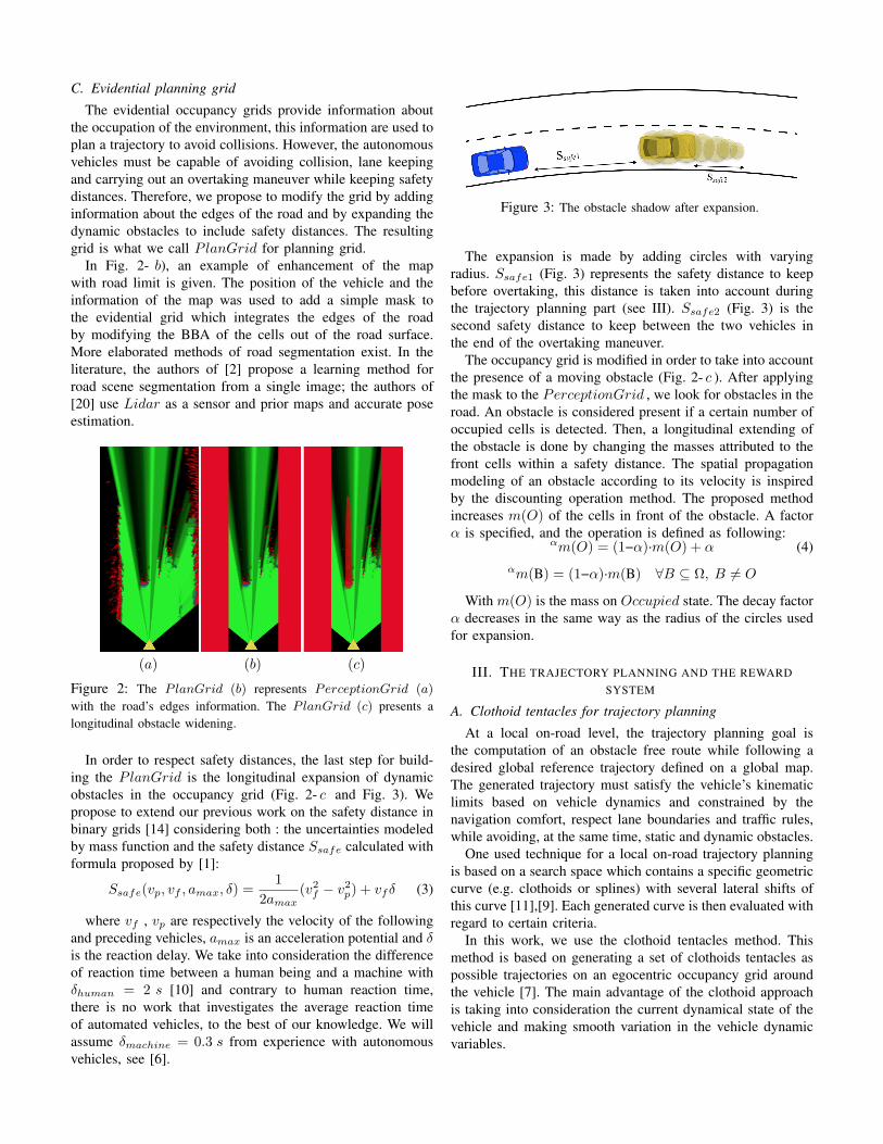
Figure 3: The obstacle shadow after expansion.

The expansion is made by adding circles with varyingradius. S

safe1 (Fig. 3) represents the safety distance to keepbefore overtaking, this distance is taken into account duringthe trajectory planning part (see III). S

safe2 (Fig. 3) is thesecond safety distance to keep between the two vehicles inthe end of the overtaking maneuver.

The occupancy grid is modified in order to take into accountthe presence of a moving obstacle (Fig. 2- c ). After applyingthe mask to the PerceptionGrid , we look for obstacles in theroad. An obstacle is considered present if a certain number ofoccupied cells is detected. Then, a longitudinal extending ofthe obstacle is done by changing the masses attributed to thefront cells within a safety distance. The spatial propagationmodeling of an obstacle according to its velocity is inspiredby the discounting operation method. The proposed methodincreases m(O) of the cells in front of the obstacle. A factor↵ is specified, and the operation is defined as following:

↵m(O) = (1−↵)·m(O) + ↵ (4)↵m(B) = (1−↵)·m(B) 8B ✓ ⌦, B 6= O

With m(O) is the mass on Occupied state. The decay factor↵ decreases in the same way as the radius of the circles usedfor expansion.

III. THE TRAJECTORY PLANNING AND THE REWARDSYSTEM

A. Clothoid tentacles for trajectory planningAt a local on-road level, the trajectory planning goal is

the computation of an obstacle free route while following adesired global reference trajectory defined on a global map.The generated trajectory must satisfy the vehicle’s kinematiclimits based on vehicle dynamics and constrained by thenavigation comfort, respect lane boundaries and traffic rules,while avoiding, at the same time, static and dynamic obstacles.

One used technique for a local on-road trajectory planningis based on a search space which contains a specific geometriccurve (e.g. clothoids or splines) with several lateral shifts ofthis curve [11],[9]. Each generated curve is then evaluated withregard to certain criteria.

In this work, we use the clothoid tentacles method. Thismethod is based on generating a set of clothoids tentacles aspossible trajectories on an egocentric occupancy grid aroundthe vehicle [7]. The main advantage of the clothoid approachis taking into consideration the current dynamical state of thevehicle and making smooth variation in the vehicle dynamicvariables.

For a fixed velocity, all tentacles begin at the center ofgravity of the vehicle and take the shape of clothoid (Fig.4).

We assume that all tentacles generated for a given speed Vx

have the same length:

Ltentacle

(m) =

(t0 Vx

� L0 Vx

> 1(m/s)

2(m) Vx

1(m/s)(5)

where t0 = 7s and L0 = 5m.The initial curvature ⇢0 of the tentacles is calculated from

the current vehicle steering angle �0 .

⇢0 =tan �0L

where L is the vehicle’s wheelbase.Tentacles of the extremity correspond respectively to the

positive and negative maximal value of the reached steeringangle which the vehicle can make at the current velocitywithout losing stability. The length of tentacles increases withthe increase of the velocity.

We assume that all tentacles generated for a given velocityhave the same length.

After generating all tentacles in the egocentred occupancygrid related to the vehicle, the next step is to choose the besttentacle to execute using different criteria.

Figure 4: Clothoid tentacles generated at the center of gravity ofthe vehicle. Red tentacles are non navigable and the yellow ones arenavigable.

B. Reward system for choosing the best tentacleAfter generating a set of tentacles, only one must be chosen

to be executed. First, a classification is made on the tentacles.They are classified as navigable or non navigable using theinformation of the occupancy grid. If a tentacle passes by anobstacle on a radius of S

safe1 in front of the ego-vehicle,this tentacle will be classified as non-navigable, otherwiseit’s navigable. If a tentacle passes by unknown cells, it’s stillconsidered navigable.

After classifying the tentacles, we evaluate the navigabletentacles using several criteria: the tentacle’s occupation, itsdistance from the global reference trajectory and the overtak-ing criterion.

To model the problem of planning with all thecriteria to be taken into consideration, we used aMarkov Decision Process (MDP ) like model [15]. AMDP is a discrete-time state-transition system. The agent(ego-vehicle) observes the state (environment around each ten-tacle) and performs an action (tentacle execution) accordingly.

The system then makes a transition to the next state and theagent receives some reward.

It can be described formally with 5 components(S,A, T,R, �): S is the set of states represented here by circlesaround the tentacles , A(s) : S ! A is the set of actions(each tentacles represents an action), T : S ⇥ S ⇥A ! [0, 1]defines the transition probabilities of the system from one stateto another when taking an action, R : S ⇥ A ! R is thereward given to each state dependung on different criteria and� ⇢ [0, 1) is the discount rate used to calculate the long-termattenuation.Reference trajectory criterion

The reference trajectory is the path that the ego-vehiclemust follow all the time. However, the ego-vehicle can deviatetemporarily from the reference trajectory to avoid obstaclesor to carry out an overtaking. We use the lateral distancebetween each tentacle and the reference trajectory to evaluatethe tentacles regarding this criterion. Details are presented in[15].Overtaking criterion

In the case of the presence of an obstacle in front of thevehicle, the tentacles of the left receive a small additionalreward since the overtaking is done by the left.Occupancy criterion

Each tentacle is evaluated in regard of its occupation. Gridinformation is used to assign appropriate rewards for eachtentacle.

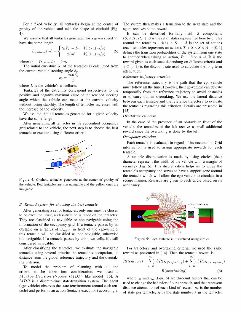
A tentacle discretization is made by using circles (theirdiameter represent the width of the vehicle with a margin ofsecurity) (Fig. 5). This discretization helps us to judge thetentacle’s occupancy and serves to have a support zone aroundthe tentacle which will allow the ego-vehicle to circulate in asecure manner. Rewards are given to each circle based on itsoccupancy.

Figure 5: Each tentacle is discretized using circles

For trajectory and overtaking criteria, we used the samereward as presented in [14]. Then the tentacle reward is:

R(tentacle) =nsX

k=0

�k

t

R(sk|trajectory) +

nsX

k=0

�k

o

R(sk|occupancy)

+R(overtaking) (6)

where �t

and �o

(Equ. 6) are discount factors that can beused to change the behavior of our approach, and that representdistance attenuation of each kind of reward. n

s

is the numberof state per tentacle, s

k

is the state number k in the tentacle.

For occupancy criterion, we used in our previous worksbinary grid with the value ’0’ for free cells and ’1’ foroccupied cells. With evidential grids, instead of having thevalue ’0’ or ’1’ in the grid cells, we dispose of mass about eachcell occupancy. Explanations on how we integrate occupancyreward will be provided in the next section.

C. Reward definition based on evidential gridWe dispose of an evidential grid in which we draw states

as circles around each tentacle. The superposition of the stateson the grid gives matrix storing belief mass values (Fig. 5).

In order to define a reward regarding the occupancy ofthe state, we propose to process cells information using fourdifferent rules. We consider that each cell is a source ofinformation about the occupancy of the state. All cells aredefined in the same frame of discernment. For each rule,we attribute a different reward (Equations 6 to 9, wherea1, a2, a3, a4 are weighting parameters):

• Conjunctive rule: the first rule consists on combiningall masses of the state matrix with conjunctive rule, theresulting mass function is m\() = \m

i

() 8 celli

2matrix.

Rewardoccupation

= a1m\(F) + a2m\(O)

+a3m\(⌦) + a4m\(/O) (7)

The conjunctive rule is used if all sources of information aretelling the truth. By applying this rule, we obtain a consensusbetween all sources of information.

• Dempster’s rule: the second rule combines all masses ofthe state matrix with Dempster’s rule, the resulting massfunction is m�() = �m

i

() 8 celli

2 matrix.Reward

occupation

= a1m�(F )+a2m�(O)+a3m�(⌦)(8)

The normalization process in Dempster’s rule has theeffect of distributing the belief of conflict to the otherpropositions, according to their respective mass.

• Mean of the masses: The third combination is amean of all masses for each state matrix m

mean

() =mean(m

i

()) 8 celli

2 matrix.Reward

occupation

= a1mmean

(F ) + a2mmean

(O)

+a3mmean

(⌦) (9)

• Cells number: with this rule, we count the number ofoccupied , free and uncertain cells of the state matrixby making a decision about their state. For that, weattribute the element A 2 2⌦ if m(A) > 0.5 .

Rewardoccupation

= a1Nb(F )+a2Nb(O)+a3Nb(⌦) (10)

IV. EXPERIMENTAL AND SIMULATION RESULTS

A. System set-up and real exampleThere are three sources in our perception system: vehicle

pose, exteroceptive acquisition data and a map. First, a glob-ally referenced pose is needed to localize the vehicle in theenvironment in terms of position and orientation comparedwith reference trajectory. The pose is provided by a GPSsystem coupled with an inertial measurement unit. Secondly,

we use a Lidar as a perception sensor. This sensor candistinguish between free and occupied space and model itin 2D (x, y coordinates) with respect to the vehicle bodyframe. We assume that we have the velocity of obstacles.In the validation tests, we used two vehicles one with theLidar sensor and the second one served as an obstacle toovertake with the velocity information. Finally, the map datawith information about the road surface are used.

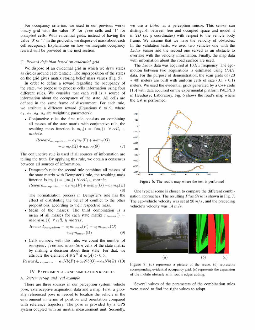
The Lidar data was acquired at 10Hz frequency. The ego-motion between two acquisitions is estimated using CANdata. For the purpose of demonstration, the scan grids of (20* 40) meters are built with uniform cells of size (0.1 * 0.1)meters. We used the evidential grids generated by a C++ code[13] with data acquired on the experimental platform PACPUSin Heudiasyc Laboratory. Fig. 6 shows the road’s map wherethe test is performed.

Figure 6: The road’s map where the test is performed

One typical scene is chosen to compare the different combi-nation approaches. The resulting PlanGrid is shown in Fig. 7.The ego-vehicle velocity was set at 20m/s , and the precedingvehicle’s velocity was 14m/s .

(a) (b) (c)

Figure 7: (a) represents a picture of the scene. (b) representscorresponding evidential occupancy grid. (c) represents the expansionof the mobile obstacle with road’s edges adding.

Several values of the parameters of the combination ruleswere tested to find the right values to adopt.

Rule a1 : 1 ! 100 a2 : �100 ! �1 a3 : �20 ! 10 a4

Conj. 10 -10 –1 –10

Demp. 50 -20 -1 –

Mean 10 -50 -1 –

Cell-N. 20 -50 –2 –

Table I: Parameters of different combination rules

B. Results with real dataDuring our tests, we collected perception data as evidential

grids. These grids have been processed with Matlab as aninput to our planning algorithm. We tested the different rulesof combination in an overtaking situation using the PlanGridof Fig. 7. The criterion used to compare them is the safetydistance at the end of the overtaking maneuver and thecalculation time.

And in order to compare with the binary grids, we transformthe PerceptionGrid (Fig. 7-b ) into a binary grid usingpignistic transformation. A cell is considered to be occupiedif betP (O) > betP (F ) , and free otherwise; with betP (O) =m(O) + 1

2m(⌦) and betP (F ) = m(F ) + 12m(⌦).

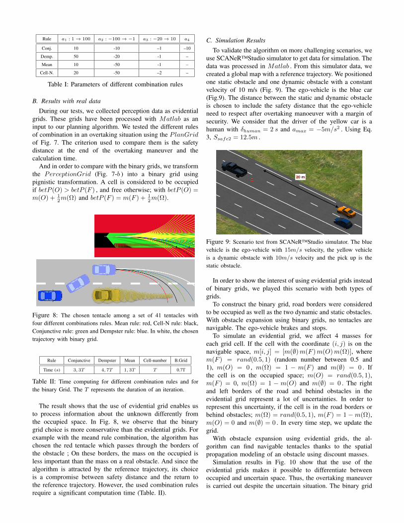
Figure 8: The chosen tentacle among a set of 41 tentacles withfour different combinations rules. Mean rule: red, Cell-N rule: black,Conjunctive rule: green and Dempster rule: blue. In white, the chosentrajectory with binary grid.

Rule Conjunctive Dempster Mean Cell-number B.Grid

Time (s) 3, 3T 4, 7T 1, 3T T 0.7T

Table II: Time computing for different combination rules and forthe binary Grid. The T represents the duration of an iteration.

The result shows that the use of evidential grid enables usto process information about the unknown differently fromthe occupied space. In Fig. 8, we observe that the binarygrid choice is more conservative than the evidential grids. Forexample with the meand rule combination, the algorithm haschosen the red tentacle which passes through the borders ofthe obstacle ; On these borders, the mass on the occupied isless important than the mass on a real obstacle. And since thealgorithm is attracted by the reference trajectory, its choiceis a compromise between safety distance and the return tothe reference trajectory. However, the used combination rulesrequire a significant computation time (Table. II).

C. Simulation ResultsTo validate the algorithm on more challenging scenarios, we

use SCANeR™Studio simulator to get data for simulation. Thedata was processed in Matlab . From this simulator data, wecreated a global map with a reference trajectory. We positionedone static obstacle and one dynamic obstacle with a constantvelocity of 10 m/s (Fig. 9). The ego-vehicle is the blue car(Fig.9). The distance between the static and dynamic obstacleis chosen to include the safety distance that the ego-vehicleneed to respect after overtaking manoeuver with a margin ofsecurity. We consider that the driver of the yellow car is ahuman with �

human

= 2 s and amax

= �5m/s2 . Using Eq.3, S

safe2 = 12.5m .

Figure 9: Scenario test from SCANeR™Studio simulator. The bluevehicle is the ego-vehicle with 15m/s velocity, the yellow vehicleis a dynamic obstacle with 10m/s velocity and the pick up is thestatic obstacle.

In order to show the interest of using evidential grids insteadof binary grids, we played this scenario with both types ofgrids.

To construct the binary grid, road borders were consideredto be occupied as well as the two dynamic and static obstacles.With obstacle expansion using binary grids, no tentacles arenavigable. The ego-vehicle brakes and stops.

To simulate an evidential grid, we affect 4 masses foreach grid cell. If the cell with the coordinate (i, j) is on thenavigable space, m[i, j] = [m(;)m(F )m(O)m(⌦)], wherem(F ) = rand(0.5, 1) (random number between 0.5 and1), m(O) = 0 , m(⌦) = 1 � m(F ) and m(;) = 0 . Ifthe cell is on the occupied space; m(O) = rand(0.5, 1),m(F ) = 0, m(⌦) = 1 � m(O) and m(;) = 0 . The rightand left borders of the road and behind obstacles in theevidential grid represent a lot of uncertainties. In order torepresent this uncertainty, if the cell is in the road borders orbehind obstacles; m(⌦) = rand(0.5, 1), m(F ) = 1 �m(⌦),m(O) = 0 and m(;) = 0 . In every time step, we update thegrid.

With obstacle expansion using evidential grids, the al-gorithm can find navigable tentacles thanks to the spatialpropagation modeling of an obstacle using discount masses.

Simulation results in Fig. 10 show that the use of theevidential grids makes it possible to differentiate betweenoccupied and uncertain space. Thus, the overtaking maneuveris carried out despite the uncertain situation. The binary grid

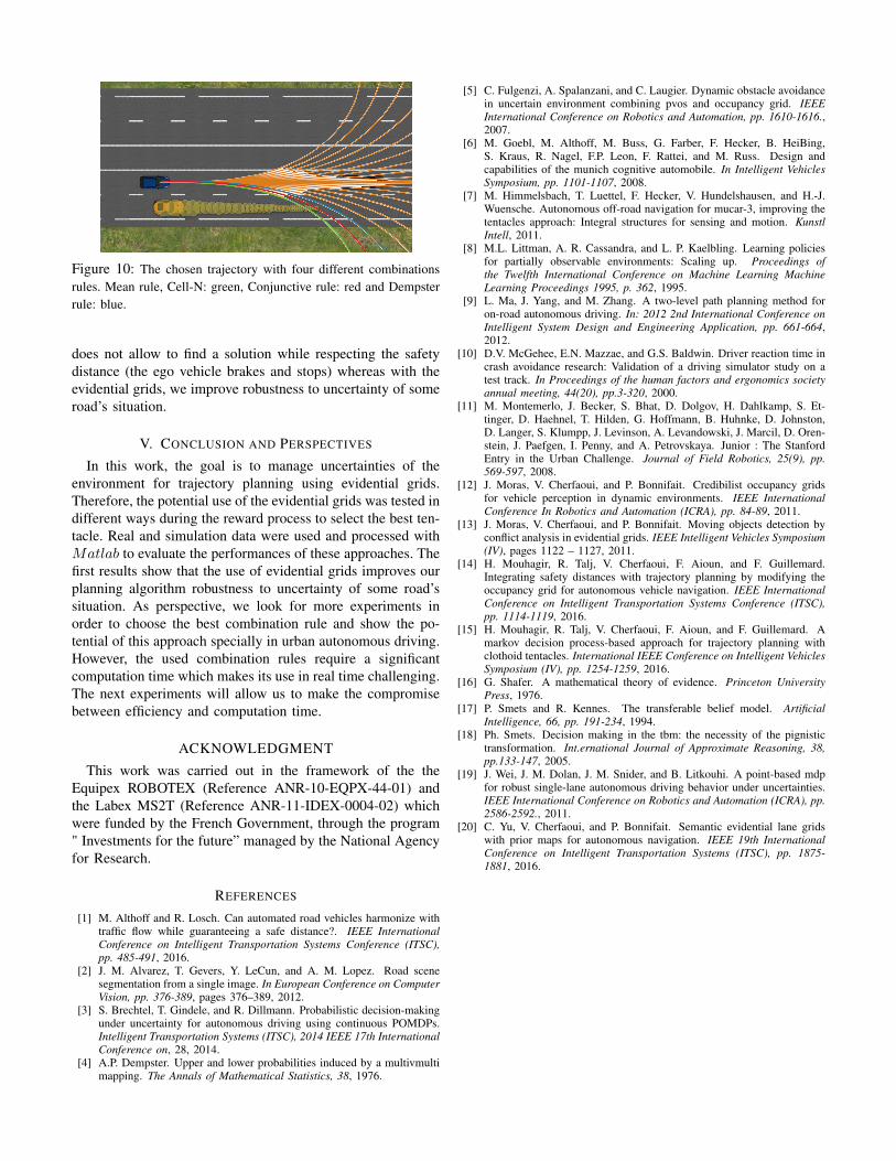
Figure 10: The chosen trajectory with four different combinationsrules. Mean rule, Cell-N: green, Conjunctive rule: red and Dempsterrule: blue.

does not allow to find a solution while respecting the safetydistance (the ego vehicle brakes and stops) whereas with theevidential grids, we improve robustness to uncertainty of someroad’s situation.

V. CONCLUSION AND PERSPECTIVES

In this work, the goal is to manage uncertainties of theenvironment for trajectory planning using evidential grids.Therefore, the potential use of the evidential grids was tested indifferent ways during the reward process to select the best ten-tacle. Real and simulation data were used and processed withMatlab to evaluate the performances of these approaches. Thefirst results show that the use of evidential grids improves ourplanning algorithm robustness to uncertainty of some road’ssituation. As perspective, we look for more experiments inorder to choose the best combination rule and show the po-tential of this approach specially in urban autonomous driving.However, the used combination rules require a significantcomputation time which makes its use in real time challenging.The next experiments will allow us to make the compromisebetween efficiency and computation time.

ACKNOWLEDGMENTThis work was carried out in the framework of the the

Equipex ROBOTEX (Reference ANR-10-EQPX-44-01) andthe Labex MS2T (Reference ANR-11-IDEX-0004-02) whichwere funded by the French Government, through the program" Investments for the future” managed by the National Agencyfor Research.

REFERENCES

[1] M. Althoff and R. Losch. Can automated road vehicles harmonize withtraffic flow while guaranteeing a safe distance?. IEEE InternationalConference on Intelligent Transportation Systems Conference (ITSC),pp. 485-491, 2016.

[2] J. M. Alvarez, T. Gevers, Y. LeCun, and A. M. Lopez. Road scenesegmentation from a single image. In European Conference on ComputerVision, pp. 376-389, pages 376–389, 2012.

[3] S. Brechtel, T. Gindele, and R. Dillmann. Probabilistic decision-makingunder uncertainty for autonomous driving using continuous POMDPs.Intelligent Transportation Systems (ITSC), 2014 IEEE 17th InternationalConference on, 28, 2014.

[4] A.P. Dempster. Upper and lower probabilities induced by a multivmultimapping. The Annals of Mathematical Statistics, 38, 1976.

[5] C. Fulgenzi, A. Spalanzani, and C. Laugier. Dynamic obstacle avoidancein uncertain environment combining pvos and occupancy grid. IEEEInternational Conference on Robotics and Automation, pp. 1610-1616.,2007.

[6] M. Goebl, M. Althoff, M. Buss, G. Farber, F. Hecker, B. HeiBing,S. Kraus, R. Nagel, F.P. Leon, F. Rattei, and M. Russ. Design andcapabilities of the munich cognitive automobile. In Intelligent VehiclesSymposium, pp. 1101-1107, 2008.

[7] M. Himmelsbach, T. Luettel, F. Hecker, V. Hundelshausen, and H.-J.Wuensche. Autonomous off-road navigation for mucar-3, improving thetentacles approach: Integral structures for sensing and motion. KunstlIntell, 2011.

[8] M.L. Littman, A. R. Cassandra, and L. P. Kaelbling. Learning policiesfor partially observable environments: Scaling up. Proceedings ofthe Twelfth International Conference on Machine Learning MachineLearning Proceedings 1995, p. 362, 1995.

[9] L. Ma, J. Yang, and M. Zhang. A two-level path planning method foron-road autonomous driving. In: 2012 2nd International Conference onIntelligent System Design and Engineering Application, pp. 661-664,2012.

[10] D.V. McGehee, E.N. Mazzae, and G.S. Baldwin. Driver reaction time incrash avoidance research: Validation of a driving simulator study on atest track. In Proceedings of the human factors and ergonomics societyannual meeting, 44(20), pp.3-320, 2000.

[11] M. Montemerlo, J. Becker, S. Bhat, D. Dolgov, H. Dahlkamp, S. Et-tinger, D. Haehnel, T. Hilden, G. Hoffmann, B. Huhnke, D. Johnston,D. Langer, S. Klumpp, J. Levinson, A. Levandowski, J. Marcil, D. Oren-stein, J. Paefgen, I. Penny, and A. Petrovskaya. Junior : The StanfordEntry in the Urban Challenge. Journal of Field Robotics, 25(9), pp.569-597, 2008.

[12] J. Moras, V. Cherfaoui, and P. Bonnifait. Credibilist occupancy gridsfor vehicle perception in dynamic environments. IEEE InternationalConference In Robotics and Automation (ICRA), pp. 84-89, 2011.

[13] J. Moras, V. Cherfaoui, and P. Bonnifait. Moving objects detection byconflict analysis in evidential grids. IEEE Intelligent Vehicles Symposium(IV), pages 1122 – 1127, 2011.

[14] H. Mouhagir, R. Talj, V. Cherfaoui, F. Aioun, and F. Guillemard.Integrating safety distances with trajectory planning by modifying theoccupancy grid for autonomous vehicle navigation. IEEE InternationalConference on Intelligent Transportation Systems Conference (ITSC),pp. 1114-1119, 2016.

[15] H. Mouhagir, R. Talj, V. Cherfaoui, F. Aioun, and F. Guillemard. Amarkov decision process-based approach for trajectory planning withclothoid tentacles. International IEEE Conference on Intelligent VehiclesSymposium (IV), pp. 1254-1259, 2016.

[16] G. Shafer. A mathematical theory of evidence. Princeton UniversityPress, 1976.

[17] P. Smets and R. Kennes. The transferable belief model. ArtificialIntelligence, 66, pp. 191-234, 1994.

[18] Ph. Smets. Decision making in the tbm: the necessity of the pignistictransformation. Int.ernational Journal of Approximate Reasoning, 38,pp.133-147, 2005.

[19] J. Wei, J. M. Dolan, J. M. Snider, and B. Litkouhi. A point-based mdpfor robust single-lane autonomous driving behavior under uncertainties.IEEE International Conference on Robotics and Automation (ICRA), pp.2586-2592., 2011.

[20] C. Yu, V. Cherfaoui, and P. Bonnifait. Semantic evidential lane gridswith prior maps for autonomous navigation. IEEE 19th InternationalConference on Intelligent Transportation Systems (ITSC), pp. 1875-1881, 2016.