Embed Size (px)
Citation preview
KIER DISCUSSION PAPER SERIES
KYOTO INSTITUTE OF
ECONOMIC RESEARCH
KYOTO UNIVERSITY
KYOTO, JAPAN
Discussion Paper No.715
“Conditional Correlations and Volatility Spillovers Between Crude Oil and Stock Index Returns”
Michael McAleer
August 2010
Conditional Correlations and Volatility Spillovers Between Crude Oil and Stock Index Returns*
Chia-Lin Chang
Department of Applied Economics National Chung Hsing University
Taichung, Taiwan
Michael McAleer Econometrics Institute
Erasmus School of Economics Erasmus University Rotterdam
and Tinbergen Institute The Netherlands
And Institute of Economic Research
Kyoto University Japan
Roengchai Tansuchat
Faculty of Economics Maejo University
Chiang Mai, Thailand
Revised: August 2010
* The authors wish to thank a referee for helpful comments and suggestions. For financial support, the first author is most grateful to the National Science Council, Taiwan, the second author thanks the Australian Research Council, National Science Council, Taiwan, and the Japan Society for the Promotion of Science, and the third author acknowledges the Faculty of Economics, Maejo University, Thailand.
1
Abstract
This paper investigates the conditional correlations and volatility spillovers between the
crude oil and financial markets, based on crude oil returns and stock index returns. Daily
returns from 2 January 1998 to 4 November 2009 of the crude oil spot, forward and futures
prices from the WTI and Brent markets, and the FTSE100, NYSE, Dow Jones and S&P500
stock index returns, are analysed using the CCC model of Bollerslev (1990), VARMA-
GARCH model of Ling and McAleer (2003), VARMA-AGARCH model of McAleer, Hoti
and Chan (2008), and DCC model of Engle (2002). Based on the CCC model, the estimates
of conditional correlations for returns across markets are very low, and some are not
statistically significant, which means the conditional shocks are correlated only in the same
market and not across markets. However, the DCC estimates of the conditional correlations
are always significant. This result makes it clear that the assumption of constant conditional
correlations is not supported empirically. Surprisingly, the empirical results from the
VARMA-GARCH and VARMA-AGARCH models provide little evidence of volatility
spillovers between the crude oil and financial markets. The evidence of asymmetric effects of
negative and positive shocks of equal magnitude on the conditional variances suggests that
VARMA-AGARCH is superior to VARMA-GARCH and CCC.
Keywards: Multivariate GARCH, volatility spillovers, conditional correlations, crude oil prices, spot, forward and futures prices, stock indices.
JEL Classifications: C22, C32, G17, G32.
2
1. Introduction
Stock market and crude oil markets have developed a mutual relationship over the past few
years, with virtually every production sector in the international economy relying heavily on
oil as an energy source. Owing to such dependence, fluctuations in crude oil prices are likely
to have significant effects on the production sector. The direct effect of an oil price shock
may be considered as an input-cost effect, with higher energy costs leading to lower oil usage
and decreases in productivity of capital and labour. Further to the direct impacts on
productivity, fluctuations in oil prices also cause income effects in the household sector, with
higher costs of imported oil reducing the disposable income of the household. Hamilton
(1983) argues that a sharp rise in oil prices increases uncertainly in the operating costs of
certain durable goods, thereby reducing demand for durables and investment.
The impact of oil prices on macroeconomic variables, such as inflation, real GDP growth
rate, unemployment rate and exchange rates, is a matter of great concern for all economies.
Due to the role of crude oil on demand and input substitution, more expensive fuel translates
into higher costs of transportation, production and heating, which affect inflation and
household discretionary spending. The literature has analysed the effects of major energy
prices, economic recession, unemployment, and inflation (see, for example, Hamilton
(1983), Mork, Olsen and Mysen (1994), Mork (1994), Lee et al. (1995), Sadorsky (1999),
Lee et al. (2001), Hooker (2002), Hamilton and Herrera (2004), Cunado and Perez de Garcia
(2005), Jimenez-Rodriguez and Senchez (2005), Kilian (2008), Cologni and Manera (2008),
and Park and Ratti (2008)). Moreover, higher prices may also reflect a stronger business
performance and increased demand for fuel.
Chang et al. (2009) explained the effect of oil price shocks on stock prices through expected
cost flows, the discount rate and the equity pricing model. However, the direction of the stock
price effect depends on whether a stock is a producer or a consumer of oil or oil-related
products. Figure 1 presents the plots of the Brent futures price and FTSE100 index from early
1998. Before 2003, the Brent futures price and FTSE100 index moved in opposite directions,
but they moved together thereafter. However, the correlation between daily Brent futures
prices and the FTSE100 index has been relatively weak at 0.162 over the past decade.
3
[Insert Figure 1 here]
Returns, risks and correlation of assets in portfolios of assets are key elements in empirical
finance, especially in developing optimal hedging strategies, so it is important to model and
forecast the correlations between crude oil and stock markets accurately. A volatility
spillover occurs when changes in price or returns volatility in one market have a lagged
impact on volatility in the financial, energy and stock markets (see, for example, Sadorsky
(2004), Hammoudeh and Aleisa (2002), Hammoudeh et al. (2004), Ågren (2006), and Malik
and Hammoudeh (2007)). Surprisingly, there does not seem to have been an analysis of the
conditional correlations or volatility spillovers between shocks in crude oil returns and in
index returns, despite these issues being very important for practitioners and investors alike.
The reaction of stock markets to oil price and returns shocks will determine whether stock
prices rationally reflect the impact of news on current and future real cash flows. The paper
models the conditional correlations and examines the volatility spillovers between two major
crude oil return, namely Brent and WTI (West Texas Intermediate) and four stock index
returns, namely FTSE100 (London Stock Exchange, FTSE), NYSE composite (New York
Stock Exchange, NYSE), S&P500 composite index, and Dow Jones Industrials (DJ). Some of
these issues have been examined empirically using several recent models of multivariate
conditional volatility, namely the CCC model of Bollerslev (1990), VARMA-GARCH model
of Ling and McAleer (2003), VARMA-AGARCH model of McAleer, Hoti and Chan (2008),
and DCC model of Engle (2002).
The remainder of the paper is organized as follows. Section 2 reviews the relationship
between the crude oil market and stock market. Section 3 discusses various popular
multivariate conditional volatility models that enable an analysis of volatility spillovers.
Section 4 gives details of the data to be in the empirical analysis, descriptive statistics and
unit root tests. The empirical results are analyzed in Section 5, and some concluding remarks
are given in Section 6
2. Crude Oil and Stock Markets
There is a scant literature on the empirical relationship between the crude oil and stock
4
markets. Jones and Kaul (1996) show the negative reaction of US, Canadian, UK and Japan
stock prices to oil price shocks via the impact of oil price shocks on real cash flows. Ciner
(2001) uses linear and nonlinear causality tests to examine the dynamic relationship between
oil prices and stock markets, and concludes that a significant relationship between real stock
returns and oil futures price is non-linear. Hammoudeh and Aleisa (2002) find spillovers from
oil markets to the stock indices of oil-exporting countries, including Bahrain, Indonesia,
Mexico and Venezuela. Kilian and Park (2009) report that only oil price increases, driven by
precautionary demand for oil over concern about future oil supplies, affect stock prices
negatively. Driesprong et al. (2008) find a strong relationship between stock market and oil
market movements.
Several previous papers have applied vector autoregressive (VAR) models to investigate the
relationship between the oil and stock markets. Kaneko and Lee (1995) find that changes in
oil prices are significant in explaining Japanese stock market returns. Huang et al. (1996)
show significant causality from oil futures prices to stock returns of individual firms, but not
to aggregate market returns. In addition, they find that oil futures returns lead the petroleum
industry stock index, and three oil company stock returns. Sadorsky (1999) indicates that
positive shocks to oil prices depress real stock returns, using monthly data, and the results
from impulse response functions suggest that oil price movements are important in explaining
movements in stock returns.
Papapetrou (2001) reveals that the oil price is an important factor in explaining stock price
movements in Greece, and that a positive oil price shock depresses real stock returns by using
impulse response functions. Lee and Ni (2002) indicate that, as a large cost share of oil
industries, such as petroleum refinery and industrial chemicals; oil price shocks tend to
reduce supply. In contrast, for many other industries, such as the automobile industry, oil
price shocks tend to reduce demand. Park and Ratti (2008) estimate the effects of oil price
shocks and oil price volatility on the real stock returns of the USA and 13 European
countries, and find that oil price shocks have a statistically significant impact on real stock
returns in the same month, and real oil price shocks also have an impact on real stock returns
across all countries. For emerging stock markets, Maghyereh (2004) finds that oil shocks
have no significant impact on stock index returns in 22 emerging economies. However,
Basher and Sadorsky (2006) show strong evidence that oil price risk has a significant impact
5
on stock price returns in emerging markets.
Regarding the relationship between oil prices and stock markets, Faff and Brailsford (1999)
find a positive impact on the oil and gas, and diversified resources, industries, whereas there
is a negative impact on the paper and packing, banks and transport industries. Sadorsky
(2001) shows that stock returns of Canadian oil and gas companies are positive and sensitive
to oil price increases using a multifactor market model. In particular, an increase in the oil
price factor increases the returns to Canadian oil and gas stocks. Boyer and Filion (2004) find
a positive association between energy stock returns and an appreciation in oil and gas prices.
Hammoudeh and Li (2005) show that oil price growth leads the stock returns of oil-exporting
countries and oil-sensitive industries in the USA.
Nandha and Faff (2007) examine the adverse effects of oil price shocks on stock market
returns using global industry indices. The empirical results indicate that oil price changes
have a negative impact on equity returns in all industries, with the exception of mining, and
oil and gas. Cong et al. (2008) argue that oil price shocks do not have a statistically
significant impact on the real stock returns of most Chinese stock market indices, except for
the manufacturing index and some oil companies. An increase in oil volatility does not affect
most stock returns, but may increase speculation in the mining and petrochemical indexes,
thereby increasing the associated stock returns. Sadorsky (2008) finds that the stock prices of
small and large firms respond fairly symmetrically to changes in oil prices, but for medium-
sized firms the response is asymmetric to changes in oil prices. From simulations using a
VAR model, Henriques and Sadorsky (2008) show that shocks to oil prices have little impact
on the stock prices of alternative energy companies.
In small emerging markets, especially in the Gulf Cooperating Council (GCC) countries,
Hammoudeh and Aleisa (2004) show that the Saudi market is the leader among GCC stock
markets, and can be predicted by oil futures prices. Maghyereh and Al-Kandari (2007) apply
nonlinear cointegration analysis to examine the linkage between oil prices and stock markets
in GCC countries. The empirical results indicate that oil prices have a nonlinear impact on
stock price indices in GCC countries. Onour (2007) argues that, in the short run, GCC stock
market returns are dominated by the influence of non-observable psychological factors. In the
long run, the effects of oil price changes are transmitted to fundamental macroeconomic
6
indicators which, in turn, affect the long run equilibrium linkages across markets.
Recent research has used multivariate GARCH specifications, especially BEKK, to model
volatility spillovers between the crude oil and stock markets. Hammoudeh et al. (2004) find
that there are two-way interactions between the S&P Oil Composite index, and oil spot and
futures prices. Malik and Hammoudeh (2007) find that Gulf equity markets receive volatility
from the oil markets, but only in the case of Saudi Arabia is the volatility spillover from the
Saudi market to the oil market significant, underlining the major role that Saudi Arabia plays
in the global oil market. Using a two-regime Markov-switching EGARCH model, Aloui and
Jammazi (2009) examine the relationship between crude oil shocks and stock markets from
December 1987 to January 2007. The paper focuses on the WTI and Brent crude oil markets
and three developed stock markets, namely France, UK and Japan. The results show that the
net oil price increase variable play a significant role in determining both the volatility of real
returns and the probability of transition across regimes.
3. Econometric Models
In order to investigate the conditional correlations and volatility spillovers between crude oil
returns and stock index returns, several multivariate conditional volatility models are used.
This section presents the CCC model of Bollerslev (1990), VARMA-GARCH model of Ling
and McAleer (2003), and VARMA-AGARCH model of McAleer, Hoti and Chan (2009).
These models assume constant conditional correlations, and do not suffer from the curse of
dimensionality, as compared with the VECH and BEKK models (see McAleer et al. (2008)
and Caporin and McAleer (2009, 2010) for further details). In order to to make the
conditional correlations time dependent, Engle (2002) proposed the DCC model.
The typical CCC specification underlying the multivariate conditional mean and conditional
variance in returns is given as follows:
( )1t t ty E y F tε−= +
t tD tε η=
( )1|t t t tVar F D Dε − t= Ω = Γ (1)
7
where , ( )1 ,...,t t mty y y ′= ( 1 ,...,t t mtη η η )′= is a sequence of independently and identically
distributed (iid) random vectors, is the past information available to time t, tF
( 1 2 1 21 ,...,t t )mtD diag h h= , m is the number of returns, 1,...,t n= (see Li, Ling and McAleer
(2002), and Bauwens et al. (2006)), and
12 1
21
1,
1 , 1
11
1
m
m m
m m m
ρ ρρ
ρρ ρ
−
−
⎛ ⎞⎜ ⎟⎜ ⎟Γ =⎜ ⎟⎜ ⎟⎜ ⎟⎝ ⎠
L
L M
M M O
L
which ij jiρ ρ= for . As , 1,...,i j m= ( ) ( )1t t t t tE F Eηη ηη−′ ′Γ = = , the constant conditional
correlation matrix of the unconditional shocks, tε , for all t is, by definition, equal to the
conditional covariance matrix of the standardized shocks, tη .
The conditional correlations are assumed to be constant for all the models above. From (1),
t t t t tD Dε ε ηη′ = ′ , and ( )1t t t t t tE F Dε ε −′ = Ω = ΓD , where tΩ is the conditional covariance
matrix. The conditional correlation matrix is defined as 1t t tD D 1− −Γ = Ω , which is assumed to
be constant over time, and each conditional correlation coefficient is estimated from the
standardized residuals in (1) and (2). The constant conditional correlation (CCC) model of
Bollerslev (1990) assumes that the conditional variance for each return, , ,
follows a univariate GARCH process, that is
ith 1,..,i m=
2,
1 1
r s
it i il i t l il i t ll j
h ω α ε β ,h− −= =
= + +∑ ∑ (2)
where 1
rill
α=∑ denotes the short run persistence, or ARCH effect, of shocks to return i,
1
sill
β=∑ represents the GARCH effect, and
1
r sij ijj j 1
α β= =
+∑ ∑ denotes the long run
persistence of shocks to returns.
8
In order to test for the existence of constant conditional correlations in the multivariate
GARCH model, Tse (2000) suggested a Lagrange Multiplier test (hereafter LMC) based on
the estimates of the CCC model. From (1), as the conditional covariances are given by
ijt ijt it jtσ ρ σ σ= ,
the equation for the time-varying correlations is defined as
, 1 , 1ijt ij ij i t j ty yρ ρ δ − −= + .
The null hypothesis of constant conditional correlations is 0 : ijH 0δ = for 1 . The
LMC test is asymptotically distributed as
i j K≤ < ≤
2Mχ , where ( 1)M K K 2= − . If the null hypothesis
is rejected, the correlations between two series are dynamic rather than static.
Although the conditional correlations can be estimated in practice, the CCC model not permit
any interdependencies of volatilities across different assets and/or markets, and does not
accommodate asymmetric behaviour. In order to incorporate interdependencies of volatilities
across different assets and/or markets, Ling and McAleer (2003) proposed a vector
autoregressive moving average (VARMA) specification of the conditional mean in (1), and
the following GARCH specification for the conditional variances:
( )( ) ( )t tL Y Lμ εΦ − = Ψ (3)
t tD tε η=
1 1
r s
t l t ll l
l t lH W A B Hε − −= =
= + +∑ ∑r (4)
where ( )1 2,t i tdiag h= ( )1 ,...,t t mt,
9
D H h h ′= , ( ) 1p
m pL I L LΦ = −Φ − −ΦL and ( ) mL IΨ = −
L )
are polynomials in L, 1q
qLΨ − −ΨL ( 2 21 ,...t mtε ε ε ′=
r , and W, for and for
are matrices and represent the ARCH and GARCH effects, respectively.
Spillover effects, or the dependence of the conditional variance between crude oil returns and
lA 1,..,l = r lB
1,..,l s= m m×
stock index returns, are given in the conditional variance for each returns in the portfolio. It is
clear that when and are diagonal matrices, (4) reduces to (2), so the VARMA-GARCH
model has CCC as a special case.
lA lB
As in the univariate GARCH model, VARMA-GARCH assumes that negative and positive
shocks of equal magnitude have identical impacts on the conditional variance. In order to
separate the asymmetric impacts of positive and negative shocks, McAleer, Hoti and Chan
(2009) proposed the VARMA-AGARCH specification for the conditional variance, namely
( )1 1 1
r r s
t l t l i t l t l l t ll l l
H W A C I B Hε η ε− − − −= = =
= + + +∑ ∑ ∑r r (5)
where are matrices for , and lC m m× 1,..,l = r ( )1diag ,...,t t mtI I I= is an indicator function,
and is given as
( )0, 01, 0
itit
it
Iε
ηε
>⎧= ⎨ ≤⎩
(6).
If , (6) collapses to the asymmetric GARCH, or GJR, model of Glosten, Jagannathan
and Runkle (1992). Moreover, VARMA-AGARCH reduces to VARMA-GARCH when
for all i. If
1m =
0iC = 0iC = and and are diagonal matrices for all i and j, then VARMA-
AGARCH reduces to CCC. The parameters of model (1)-(5) are obtained by maximum
likelihood estimation (MLE) using a joint normal density. When
iA jB
tη does not follow a joint
multivariate normal distribution, the appropriate estimator is the Quasi-MLE (QMLE).
Unless tη is a sequence of iid random vectors, or alternatively a martingale difference
process, the assumption that the conditional correlations are constant may seen unrealistic. In
order to make the conditional correlation matrix time dependent, Engle (2002) proposed a
dynamic conditional correlation (DCC) model, which is defined as
10
1| (0,t t t )y Q−ℑ , 1,2,...,=t n (7)
,= Γt t t tQ D D (8)
where ( ) 1 2diagt tD h= ⎡ ⎤⎣ ⎦
,h
is a diagonal matrix of conditional variances, and is the
information set available to time t. The conditional variance, , can be defined as a
univariate GARCH model, as follows:
tℑ
ith
,1 1
p q
it i ik i t k il i t lk l
h ω α ε β− −= =
= + +∑ ∑ . (9)
If tη is a vector of i.i.d. random variables, with zero mean and unit variance, in (8) is the
conditional covariance matrix (after standardization,
tQ
it it ityη = h ). The itη are used to
estimate the dynamic conditional correlations, as follows:
{ } { }1/2 1/2( ( ) ( ( )t t t tdiag Q Q diag Q−Γ = −
t
(10)
where the k symmetric positive definite matrix Q is given by k×
1 2 1 1 1 2(1 )t t tQ Qθ θ θ η η θ 1tQ− −′= − − + + − (11)
in which 1θ and 2θ are non-negative scalar parameters to capture, respectivey, the effects of
previous shocks and previous dynamic conditional correlations on the current dynamic
conditional correlation. As is a conditional on the vector of standardized residuals, (11) is
a conditional covariance matrix, and
tQ
Q is the k k× unconditional variance matrix of tη . For
further details, and a critique of DCC and BEKK, see Caporin and McAleer (2009, 2010).
4. Data
For the empirical analysis, daily data are used for the four indexes, namely FTSE100
(London Stock Exchange: FTSE), NYSE composite (New York Stock Exchange: NYSE),
S&P500 composite (Standard and Poor’s: S&P), and Dow Jones Industrials (Dow Jones: DJ),
11
and three crude oil closing prices (spot, forward and futures) of two reference markets,
namely Brent and WTI (West Texas Intermediate). Thus, there are six price indexes, namely
Brent spot prices FOB (BRSP), Brent one-month forward prices (BRFOR), Brent one-month
futures prices (BRFU), WTI spot Cushing prices (WTISP), WTI one-month forward price
(WTIFOR), and NYMEX one month futures price (WTIFU). All 3,090 prices and price index
observations are from 2 January 1998 to 4 November 2009. The data are obtained from
DataStream database services, and crude oil prices are expressed in USD per barrel.
The returns of the daily price index and crude oil prices are calculated by a continuous
compound basis, defined as ( ), ,lnij t ij t ij tr P P , 1−= , where and ,ij tP , 1ij tP − are the closing price or
crude oil price i of market j for days t and t –1, respectively. The daily prices and daily
returns of each crude oil prices, and for the four set index, are given in Figures 1 and 2,
respectively. The plots of the prices and returns in their respective markets clearly move in a
similar manner. The descriptive statistics for the crude oil returns and set index returns are
reported in Tables 1 and 2, respectively. The average returns of the set index are low, except
for Dow Jones, but the corresponding standard deviation of returns is much higher. On the
contrary, the average returns of crude oil are the same within their markets, and are higher
than the average return of the set index. Based on the standard deviation, crude oil returns has
a higher historical volatility than stock index returns.
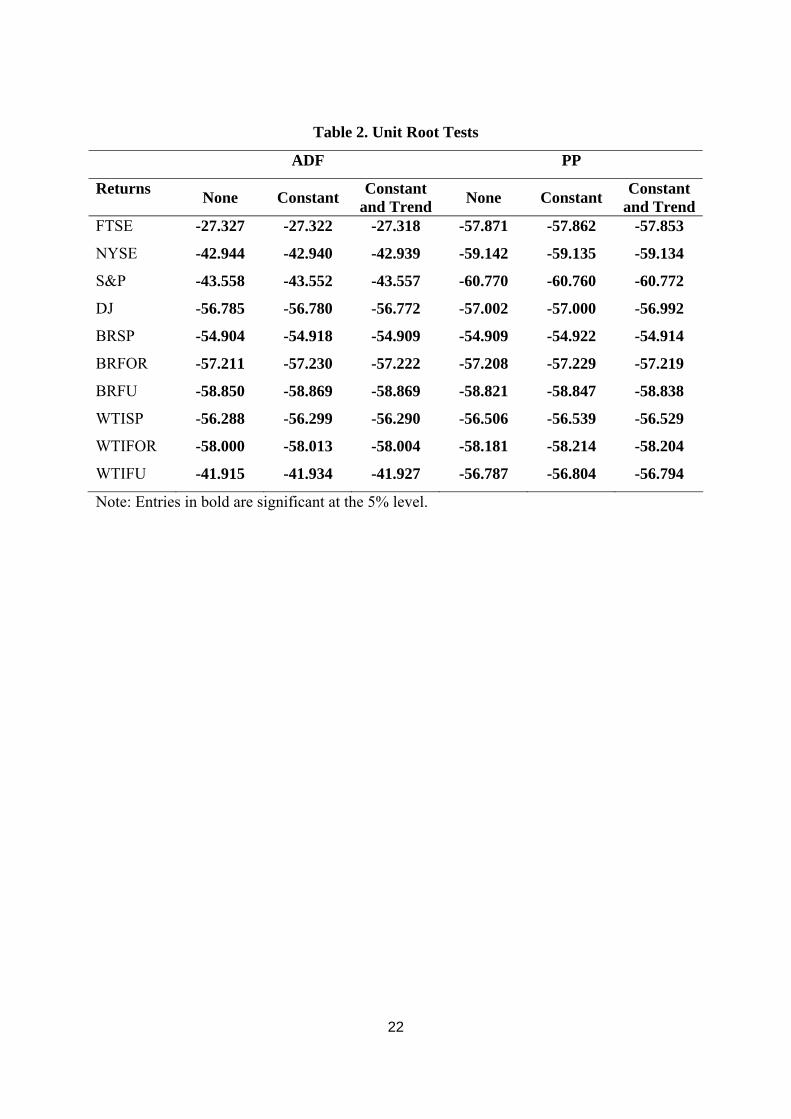
Prior to estimating the condition mean or conditional variance, it is sensible to test for unit
roots in the series. Standard unit root testing procedures based on the Augmented Dickey-
Fuller (ADF) and Phillips and Perron (PP) tests are obtained from the EViews 6.0
econometric software package. Results of the tests for the null hypothesis that daily stock
index returns and crude oil returns have a unit root are given in Table 2, and all reject the null
hypothesis of a unit root at the 1% level of significance, both with a constant and with or
without a deterministic time trend.
5. Empirical Results
This section presents the multivariate conditional volatility models for six crude oil returns,
namely spot, forward and futures for the Brent and WTI markets, and four stock index
returns, namely FTSE100, NYSE, Dow Jones and S&P, leading to 24 bivariate models. In
12
order to check whether the conditional variances of the assets follow an ARCH process,
univariate ARMA-GARCH and ARMA-GJR models are estimated. The ARCH and GARCH
effects of all ARMA(1,1)-GARCH (1,1) models are statistically significant, as are the
asymmetric effects of the ARMA-GJR(1,1) models. The empirical results of these univariate
conditional volatility models are available from the authors on request.
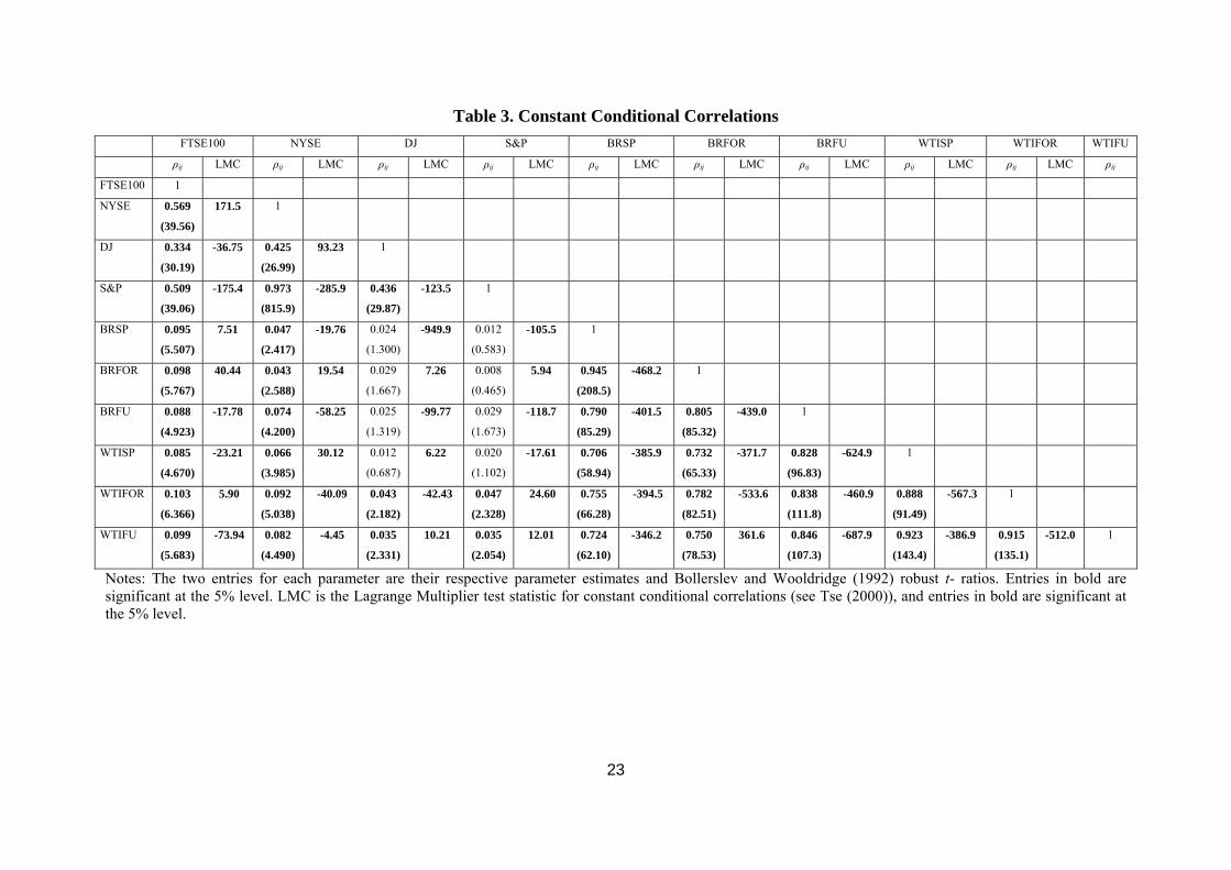
Constant conditional correlations between the volatilities of crude oil returns and stock index
returns, the Bollerslev and Wooldridge (1992) robust t-ratios using the CCC model based on
ARMA(1,1)-CCC(1,1), and the LMC test statistics, are presented in Table 3. All estimates
are obtained using the RATS 6.2 econometric software package. The conditional correlation
matrices for the 24 pairs of returns can be divided into three groups, namely within crude oil
markets, financial or stock markets, and across markets. The CCC estimates for pairs of crude
oil returns within the crude oil market are high and statistically significant, as well as the
estimates for pairs of stock index returns in financial markets. However, the CCC estimates
for returns across markets are very low, and some are not statistically significant. Thus, the
conditional shocks are correlated only in the same market, and not across markets.
[Insert Table 3 here]
The LMC test statistic is significant at the 5% level, so that the conditional correlations
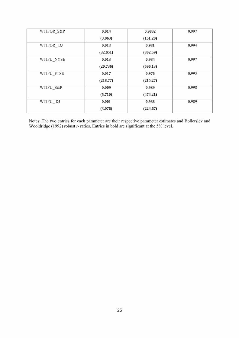
between any two series are time varying. The DCC estimates of the conditional correlations
between the volatilities of crude oil returns and stock index returns, and the Bollerslev-
Wooldridge robust t-ratios based on the ARMA(1,1)-DCC(1,1) models, are presented in
Table 4. As the estimates of both 1̂θ , the impact of past shocks on current conditional
correlations, and 2̂θ , the impact of previous dynamic conditional correlations, are
statistically significant, this also indicates that the conditional correlations are not constant.
The estimates 1̂θ are generally low and close to zero, increasing to 0.021, whereas the
estimates 2̂θ are extremely high and close to unity, ranging from 0.973 to 0.991. Therefore,
from (11), seems to be very close to tQ 1tQ − , such as for the pair WTIFOR and FTSE.
[Insert Table 4 here]
13
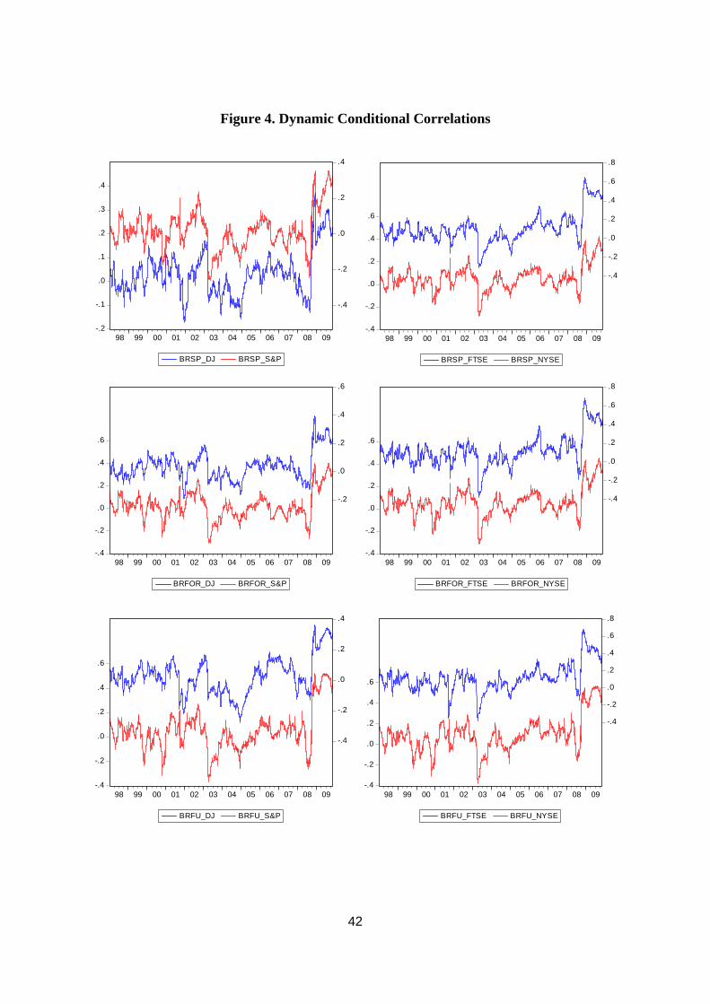
The short run persistence of shocks on the dynamic conditional correlations is the greatest
between BRFOR_FTSE, while the largest long run persistence of shocks on the conditional
correlations is 0.998 for the pairs WTIFOR_FTSE and WTIFU_S&P. Thus, the conditional
correlations between crude oil returns and stock index returns are dynamic. These findings
are consistent with the plots of the dynamic conditional correlations between the standardized
shocks for each pair of returns in Figure 4, which change over time and range from negative
to positive. The greatest range of conditional correlations is between Brent forward returns
and FTSE100. These results indicate that the assumption of constant conditional correlations
for all shocks to returns is not supported empirically. However, the mean conditional
correlations for each pair are nevertheless rather low and close to zero.
[Insert Table 5 here]
[Insert Figure 4 here]
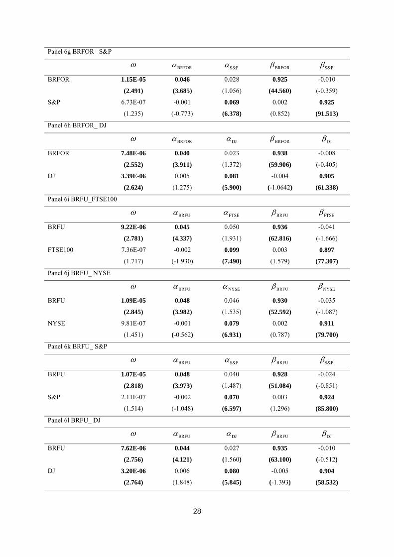
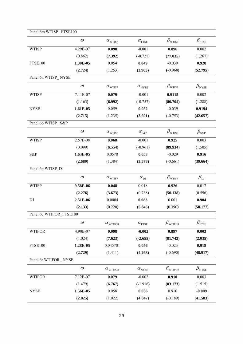
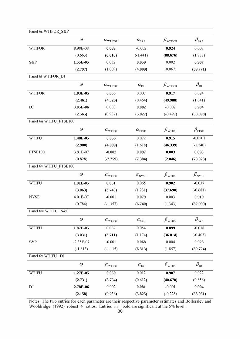
Tables 6 and 7 present the estimates for VARMA-GARCH and VARMA-AGARCH,
respectively. The two entries corresponding to each of the parameters are the estimates and
the Bollerslev-Wooldridge robust t-ratios. Both models are estimated with the EViews 6.0
econometric software package and the Berndt-Hall-Hall-Hausman (BHHH) algorithm. Table
6 presents the estimates of the conditional variances of VARMA-GARCH (the estimates of
the conditional means are available from the authors on request). In Panels 5a-5w, it is clear
that the ARCH and GARCH effects of crude oil returns and stock index returns in the
conditional covariances are statistically significant. Interestingly, Table 6 suggests there is no
evidence of volatility spillovers in one or two directions (namely, interdependence), except
for two cases, namely the ARCH and GARCH effects for WTIFOR_FTSE100 and
WTIFU_FTSE100, with the past conditional volatility of FTSE100 spillovers for WTIFOR,
and the past conditional volatility of WTIFU spillovers for FTSE100.
[Insert Table 6 here]
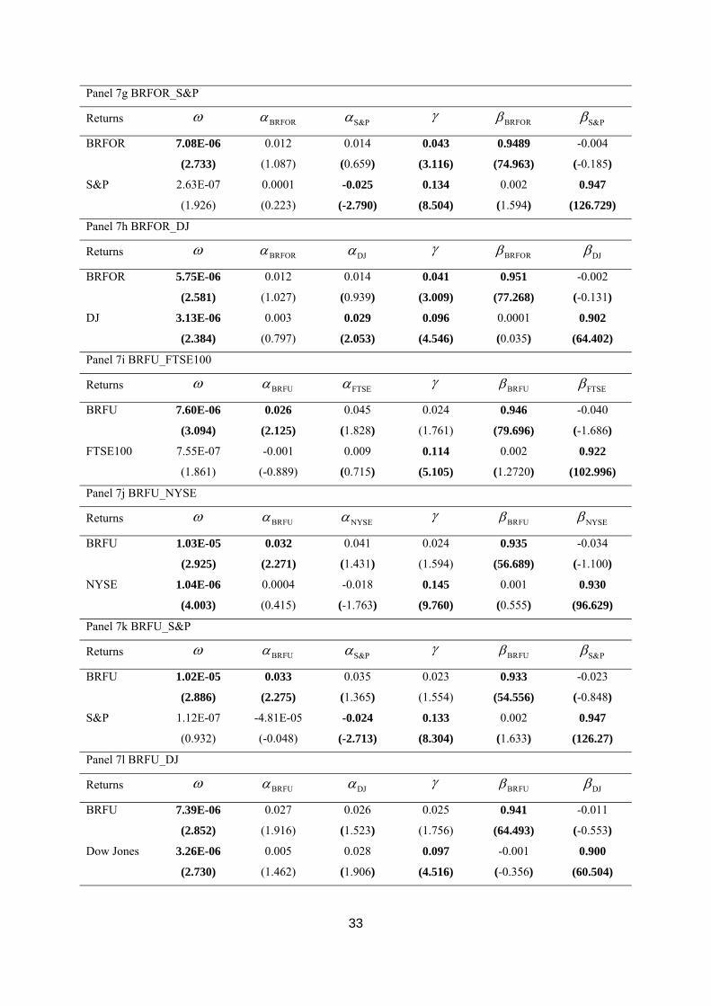
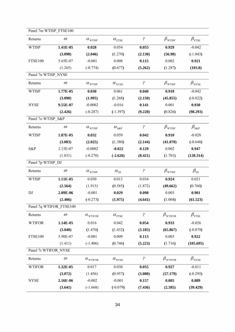
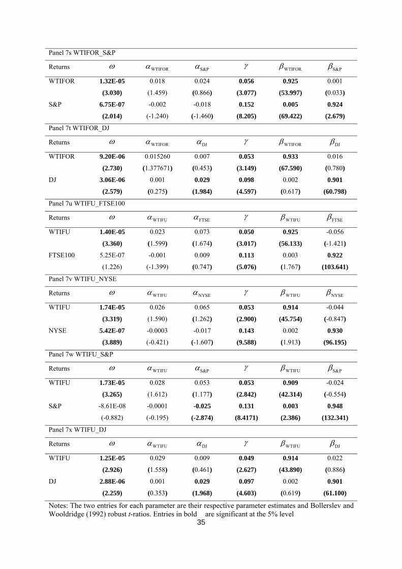
Table 7 presents the estimates of the conditional variances of VARMA-AGARCH (estimates
of the conditional mean are available from the authors on request). The GARCH effect of
each pair of crude oil returns and stock index returns in the conditional covariances are
statistically significant. Surprisingly, Table 7 shows that there are only 3 of 24 cases for
14
volatility spillovers from the past conditional volatility of the crude oil market on the stock
market, namely WTIFOR-NYSE, WTIFOR-S&P and WTIFU-S&P. The estimated
parameters are positive but also low, and the asymmetric effects of each pair are statistically
insignificant. Therefore, VARMA-GARCH is generally preferred to VARMA-AGARCH.
[Insert Table 7 here]
In conclusion, from the VARMA-GARCH and VARMA-AGARCH models, there is little
evidence of volatility spillovers between crude oil returns and stock index returns. These
finding are consistent with the very low conditional correlations between the volatility of
crude oil returns and stock index returns using the CCC model. These phenomena can be
explained as follows. First, as the stock market index is calculated from the given company
stock prices, which can be classified as producers and consumers of oil and oil-related
companies, the impact of crude oil shocks on each stock index sector may balance out. For
example, the energy sector, namely oil and gas drilling and exploration, refining and by-
products, and petrochemicals, is typically positively affected by variations in oil prices,
whereas the other sectors, such as manufacturing, transportation and financial sectors, are
negatively affected by variations in oil prices.
Second, each common stock price in the stock index is not affected equally or
contemporaneously by fluctuations in oil prices. The service sectors, namely media,
entertainment, support services, hotel and transportation, are most negatively affected by
fluctuations in oil prices, followed by the consumer goods sector, namely household goods
and beverages, housewares and accessories, automobile and parts, and textiles. The next most
negatively influenced sector is the financial sector, namely banks, life, assurance, insurance,
real estate, and other finance. Consequently, the impacts of crude oil changes on stock index
returns may not be immediate or explicit. Third, through advances in financial instruments,
some firms may have found ways to pass on oil prices changes or risks to customers, or
determined effective hedging strategies. Therefore, the effects of crude oil price fluctuations
on stock prices may not be as large as might be expected.
6. Concluding Remarks
15

This paper investigated conditional correlations and examined the volatility spillovers
between crude oil returns, namely spot, forward and futures returns for the WTI and Brent
markets, and stock index returns, namely FTSE100, NYSE, Dow Jones and S&P index, using
four multivariate GARCH models, namely the CCC model of Bollerslev (1990), VARMA-
GARCH model of Ling and McAleer (2003), VARMA-AGARCH model of McAleer, Hoti
and Chan (2008), and DCC model of Engle (2002), with a sample size of 3089 returns
observations from 2 January 1998 to 4 November 2009. The estimation and analysis of the
volatility and conditional correlations between crude oil returns and stock index returns can
provide useful information for investors, oil traders and government agencies that are
concerned with the crude oil and stock markets. The empirical results will also be able to
assist in evaluating the impact of crude oil price fluctuations on various stock markets.
Based on the CCC model, the estimated conditional correlations for returns across markets
were very low, and some were not statistically significant, which means that the conditional
shocks were correlated only in the same market, and not across markets. However, for the
DCC model, the estimates of the conditional correlations were always significant, which
makes it clear that the assumption of constant conditional correlations was not supported
empirically. This was highlighted by the dynamic conditional correlations between Brent
forward returns and FTSE100, which varied dramatically over time.
The empirical results from the VARMA-GARCH and VARMA-AGARCH models provided
little evidence of dependence between the crude oil and financial markets. VARMA-GARCH
model yielded only 2 of 24 cases, namely WTIFU_FTSE100 and WTIFU_FTSE100, whereas
VARMA-AGARCH gave 3 of 24 cases, namely the past conditional volatility of FTSE100
spillovers to WTIFOR, and the past conditional volatility of WTIFU spillovers to FTSE100.
The evidence of asymmetric effects of negative and positive shocks of equal magnitude on
the conditional variance suggested that VARMA-AGARCH was superior to the VARMA-
GARCH and CCC models.
16
References Aloui, C. and R. Jammazi (2009), The effects of crude oil shocks on stock market shifts
behavior: A regime switching approach, Energy Economics, 31, 789-799.
Arouri, M. and J. Fouquau (2009), On the short-term influence of oil price changes on stock
markets in GCC countries: linear and nonlinear analyses. Available at
http://arxiv.org/abs/0905.3870.
Basher, S.A. and P. Sardosky (2006), Oil price risk and emerging stock markets, Global
Finance Journal, 17, 224-251.
Bauwens, L., S. Laurent and J. Rombouts (2006), Multivariate GARCH models: A survey,
Journal of Applied Econometrics, 21, 79-109.
Bollerslev, T. (1990), Modelling the coherence in short-run nominal exchange rate: A
multivariate generalized ARCH approach, Review of Economics and Statistics 72,
498-505.
Bollerslev, T. and J. Wooldridge (1992), Quasi-maximum likelihood estimation and inference
in dynamic models with time-varying covariances, Econometric Reviews, 11, 143-
172.
Boyer, M. and D. Filion (2004), Common and fundamental factors in stock returns of
Canadian oil and gas companies, Energy Economics, 29, 428-453.
Caporin, M. and M. McAleer (2009), Do we really need both BEKK and DCC? A tale of two
covariance models. Available at SSRN: http://ssrn.com/abstract=1338190.
Caporin, M. and M. McAleer (2010), Do we really need both BEKK and DCC? A tale of two
multivariate GARCH models. Available at SSRN: http://ssrn.com/abstract=1549167.
Chang, C.-L., M. McAleer and R. Tansuchat (2009), Volatility spillovers between returns on
crude oil futures and oil company stocks. Available at
http://ssrn.com/abstract=1406983.
Ciner, C. (2001), Energy shocks and financial markets: nonlinear linkages, Studies in
Nonlinear Dynamics & Econometrics, 5(3), 203-212.
Cologni, A. and M. Manera (2008), Oil prices, inflation and interest rates in a structural
cointegrated VAR model for the G-7 countries, Energy Economics, 38, 856–888.
Cong, R.-G., Y.-M. Wei, J.-L. Jiao and Y. Fan (2008), Relationships between oil price shocks
and stock market: An empirical analysis from China, Energy Policy, 36, 3544-3553.
Cunado, J. and F. Perez de Garcia (2005), Oil prices, economic activity and inflation:
Evidence for some Asian countries, Quarterly Review of Economics and Finance,
17
45(1), 65–83.
Driesprong, G., B. Jacobsen and B. Maat (2008), Striking oil: Another puzzle?, Journal of
Financial Economics, 89, 307-327.
Engle, R. (2002), Dynamic conditional correlation: A simple class of multivariate generalized
autoregressive conditional heteroskedasticity models, Journal of Business and
Economic Statistics, 20, 339-350.
Faff, R.W. and T. Brailsford (1999), Oil price risk and the Australian stock market, Journal
of Energy Finance and Development, 4, 69-87.
Glosten, L., R. Jagannathan and D. Runkle (1992), On the relation between the expected
value and volatility of nominal excess return on stocks, Journal of Finance, 46, 1779-
1801.
Gogineni, S. (2009), Oil and the stock market: An industry level analysis, Working paper,
University of Oklahoma.
Hamilton, J.D. (1983), Oil and the macroeconomy since World War II, Journal of Political
Economy, 88, 829-853.
Hamilton, J.D. and A.M. Herrera (2004), Oil shocks and aggregate macroeconomic behavior:
the role of monetary policy, Journal of Money, Credit and Banking, 36 (2), 265-286.
Hammoudeh, S. and E. Aleisa (2002), Relationship between spot/futures price of crude oil
and equity indices for oil-producing economies and oil-related industries, Arab
Economic Journal, 11, 37-62.
Hammoudeh, S. and E. Aleisa (2004), Dynamic relationships among GCC stock markets and
NYMEX oil futures, Contemporary Economics Policy, 22, 250-269.
Hammoudeh, S., S. Dibooglu and E. Aleisa (2004), Relationships among US oil prices and
oil industry equity indices, International Review of Economics and Finance, 13(3),
427-453.
Hammoudeh, S. and H. Li (2005), Oil sensitivity and systematic risk in oil-sensitive stock
indices, Journal of Economics and Business, 57, 1-21.
Henriques, I. and P. Sadorsky (2008), Oil prices and the stock prices of alternative energy
companies, Energy Economics, 30, 998-1010.
Hooker, M. (2002), Are oil shocks inflationary? Asymmetric and nonlinear specification
versus changes in regime, Journal of Money, Credit and Banking, 34(2), 540-561.
Huang, R.D., R.W. Masulis and H.R. Stoll (1996), Energy shocks and financial markets,
Journal of Futures Markets, 16(1), 1-27.
18
Jiménez-Rodríguez, R. and M. Sánchez (2005), Oil price shocks and real GDP growth:
Empirical evidence for some OECD countries, Applied Economics, 37(2), 201-228.
Jones, C.M. and G. Kaul (1996), Oil and the stock markets, Journal of Finance, 51(2), 463-
491.
Kaneko, T. and B.-S. Lee (1995), Relative importance of economic factors in the U.S. and
Japanese stock markets, Journal of the Japanese and International Economics, 9,
290-307.
Kilian, L. (2008), A comparison of the effects of exogenous oil supply shocks on output and
inflation in the G7 countries, Journal of the European Economic Association, 6(1),
78–121.
Kilian, L. and C. Park (2009), The impact of oil price shocks on the U.S. stock market,
International Economic Review, 50, 1267-1287.
Lee, K., S. Ni and R.A. Ratti (1995), Oil shocks and the macroeconomy: The role of price
variability, Energy Journal, 16, 39-56.
Lee, B.R., K. Lee and R.A. Ratti (2001) Monetary policy, oil price shocks, and the Japanese
economy, Japan and the World Economy, 13, 321–349.
Lee, K. and S. Ni (2002), On the dynamic effects of oil price shocks: a study using industry
level data, Journal of Monetary Economics, 49, 823-852.
Li, W.-K., S. Ling and M. McAleer (2002), Recent theoretical results for time series models
with GARCH errors, Journal of Economic Surveys, 16, 245-269. Reprinted in M.
McAleer and L. Oxley (eds.), Contributions to Financial Econometrics: Theoretical
and Practical Issues, Blackwell, Oxford, 2002, pp. 9-33.
Ling, S. and M. McAleer (2003), Asymptotic theory for a vector ARMA-GARCH model,
Econometric Theory, 19, 278-308.
Maghyereh, A. (2004), Oil price shocks and emerging stock markets: A generalized VAR
approach, International Journal of Applied Econometrics and Quantitative Studies,
1(2), 27-40.
Maghyereh, A. and A. Al-Kandari (2007), Oil prices and stock markets in GCC countries:
New evidence from nonlinear cointegration analysis, Managerial Finance, 33(7),
449-460.
Malik, F. and S. Hammoudeh (2007), Shock and volatility transmission in the oil, US and
Gulf equity markets, International Review of Economics and Finance, 16, 357-368.
McAleer, M., F. Chan, S. Hoti and O. Lieberman (2008), Generalized autoregressive
19
conditional correlation, Econometric Theory, 24, 1554-1583.
McAleer, M., S. Hoti and F. Chan (2009), Structure and asymptotic theory for multivariate
asymmetric conditional volatility, Econometric Reviews, 28, 422-440.
Mork, K. (1994), Business cycles and the oil market, Energy Journal, 15, 15-38.
Mork, K.A., O. Olsen and H.T. Mysen (1994), Macroeconomic responses to oil price
increases and decreases in seven OECD countries, Energy Journal, 15: 19–35.
Nandha, M. and R. Faff (2007), Does oil move equity prices? A global view, Energy
Economics, 30, 986-997.
Onour, I. (2007), Impact of oil price volatility on Gulf Cooperation Council stock markets’
return, Organization of the Petroleum Exporting Countries, 31, 171-189.
Papapetrou, E. (2001), Oil price shocks, stock markets, economic activity and employment in
Greece, Energy Economics, 23, 511-532.
Park, J. and R.A. Ratti (2008), Oil price shocks and stock markets in the U.S. and 13
European countries, Energy Economics, 30, 2587-2608.
Sadorsky, P. (1999), Oil price shocks and stock market activity, Energy Economics, 21, 449-
469.
Sadorsky, P. (2001), Risk factors in stock returns of Canadian oil and gas companies, Energy
Economics, 23, 17-28.
Sadorsky, P. (2004), Stock markets and energy prices, Encyclopedia of Energy, Vol. 5,
Elsevier, New York, 707−717.
Sadorsky, P. (2008), Assessing the impact of oil prices on firms of different sizes: Its tough
being in the middle, Energy Policy, 36, 3854–3861.
Tse, Y.K. (2000), A test for constant correlations in a multivariate GARCH models, Journal
of Econometrics, 98, 107-127.
20
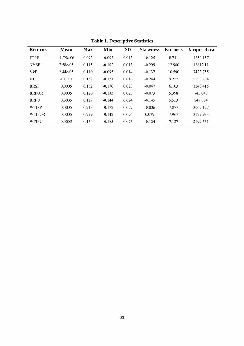
Table 1. Descriptive Statistics
Returns Mean Max Min SD Skewness Kurtosis Jarque-Bera FTSE -1.75e-06 0.093 -0.093 0.013 -0.125 8.741 4250.157
NYSE 7.58e-05 0.115 -0.102 0.013 -0.299 12.960 12812.11
S&P 2.44e-05 0.110 -0.095 0.014 -0.137 10.590 7423.755
DJ -0.0001 0.132 -0.121 0.016 -0.244 9.227 5020.704
BRSP 0.0005 0.152 -0.170 0.023 -0.047 6.103 1240.415
BRFOR 0.0005 0.126 -0.133 0.023 -0.073 5.398 743.048
BRFU 0.0005 0.129 -0.144 0.024 -0.145 5.553 849.874
WTISP 0.0005 0.213 -0.172 0.027 -0.006 7.877 3062.127
WTIFOR 0.0005 0.229 -0.142 0.026 0.099 7.967 3179.933
WTIFU 0.0005 0.164 -0.165 0.026 -0.124 7.127 2199.531
21
22
Table 2. Unit Root Tests
ADF PP
Returns None Constant Constant and Trend None Constant Constant
and TrendFTSE -27.327 -27.322 -27.318 -57.871 -57.862 -57.853
NYSE -42.944 -42.940 -42.939 -59.142 -59.135 -59.134
S&P -43.558 -43.552 -43.557 -60.770 -60.760 -60.772
DJ -56.785 -56.780 -56.772 -57.002 -57.000 -56.992
BRSP -54.904 -54.918 -54.909 -54.909 -54.922 -54.914
BRFOR -57.211 -57.230 -57.222 -57.208 -57.229 -57.219
BRFU -58.850 -58.869 -58.869 -58.821 -58.847 -58.838
WTISP -56.288 -56.299 -56.290 -56.506 -56.539 -56.529
WTIFOR -58.000 -58.013 -58.004 -58.181 -58.214 -58.204
WTIFU -41.915 -41.934 -41.927 -56.787 -56.804 -56.794
Note: Entries in bold are significant at the 5% level.
23
Table 3. Constant Conditional Correlations FTSE100 NYSE DJ S&P BRSP BRFOR BRFU WTISP WTIFOR WTIFU
ρij LMC ρij LMC ρij LMC ρij LMC ρij LMC ρij LMC ρij LMC ρij LMC ρij LMC ρij
FTSE100 1
NYSE 0.569
(39.56)
171.5 1
DJ 0.334
(30.19)
-36.75 0.425
(26.99)
93.23 1
S&P 0.509
(39.06)
-175.4 0.973
(815.9)
-285.9 0.436
(29.87)
-123.5 1
BRSP 0.095
(5.507)
7.51 0.047
(2.417)
-19.76 0.024
(1.300)
-949.9 0.012
(0.583)
-105.5 1
BRFOR 0.098
(5.767)
40.44 0.043
(2.588)
19.54 0.029
(1.667)
7.26 0.008
(0.465)
5.94 0.945
(208.5)
-468.2 1
BRFU 0.088
(4.923)
-17.78 0.074
(4.200)
-58.25 0.025
(1.319)
-99.77 0.029
(1.673)
-118.7 0.790
(85.29)
-401.5 0.805
(85.32)
-439.0 1
WTISP 0.085
(4.670)
-23.21 0.066
(3.985)
30.12 0.012
(0.687)
6.22 0.020
(1.102)
-17.61 0.706
(58.94)
-385.9 0.732
(65.33)
-371.7 0.828
(96.83)
-624.9 1
WTIFOR 0.103
(6.366)
5.90 0.092
(5.038)
-40.09 0.043
(2.182)
-42.43 0.047
(2.328)
24.60 0.755
(66.28)
-394.5 0.782
(82.51)
-533.6 0.838
(111.8)
-460.9 0.888
(91.49)
-567.3 1
WTIFU 0.099
(5.683)
-73.94 0.082
(4.490)
-4.45 0.035
(2.331)
10.21 0.035
(2.054)
12.01 0.724
(62.10)
-346.2 0.750
(78.53)
361.6 0.846
(107.3)
-687.9 0.923
(143.4)
-386.9 0.915
(135.1)
-512.0 1
Notes: The two entries for each parameter are their respective parameter estimates and Bollerslev and Wooldridge (1992) robust t- ratios. Entries in bold are significant at the 5% level. LMC is the Lagrange Multiplier test statistic for constant conditional correlations (see Tse (2000)), and entries in bold are significant at the 5% level.
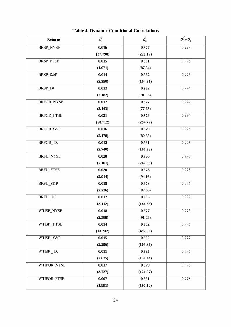
Table 4. Dynamic Conditional Correlations
Returns 1̂θ 2̂θ 1 2늿+θ θ
BRSP_NYSE 0.016
(27.798)
0.977
(228.17)
0.993
BRSP_FTSE 0.015
(1.971)
0.981
(87.34)
0.996
BRSP_S&P 0.014
(2.350)
0.982
(104.21)
0.996
BRSP_DJ 0.012
(2.182)
0.982
(91.63)
0.994
BRFOR_NYSE 0.017
(2.143)
0.977
(77.63)
0.994
BRFOR_FTSE 0.021
(68.712)
0.973
(294.77)
0.994
BRFOR_S&P 0.016
(2.178)
0.979
(80.85)
0.995
BRFOR_ DJ 0.012
(2.740)
0.981
(106.38)
0.993
BRFU_NYSE 0.020
(7.161)
0.976
(267.55)
0.996
BRFU_FTSE 0.020
(2.914)
0.973
(94.16)
0.993
BRFU_S&P 0.018
(2.226)
0.978
(87.66)
0.996
BRFU_ DJ 0.012
(3.112)
0.985
(186.65)
0.997
WTISP_NYSE 0.018
(2.388)
0.977
(91.03)
0.995
WTISP _FTSE 0.014
(13.232)
0.982
(497.96)
0.996
WTISP _S&P 0.015
(2.256)
0.982
(109.66)
0.997
WTISP _ DJ 0.011
(2.625)
0.985
(150.44)
0.996
WTIFOR_NYSE 0.017
(3.727)
0.979
(121.97)
0.996
WTIFOR_FTSE 0.007
(1.991)
0.991
(197.10)
0.998
24
WTIFOR_S&P 0.014
(3.063)
0.9832
(151.20)
0.997
WTIFOR_ DJ 0.013
(32.651)
0.981
(302.59)
0.994
WTIFU_NYSE 0.013
(20.736)
0.984
(596.13)
0.997
WTIFU_FTSE 0.017
(218.77)
0.976
(215.27)
0.993
WTIFU_S&P 0.009
(5.710)
0.989
(474.21)
0.998
WTIFU_ DJ 0.001
(3.076)
0.988
(224.67)
0.989
Notes: The two entries for each parameter are their respective parameter estimates and Bollerslev and Wooldridge (1992) robust t- ratios. Entries in bold are significant at the 5% level.
25
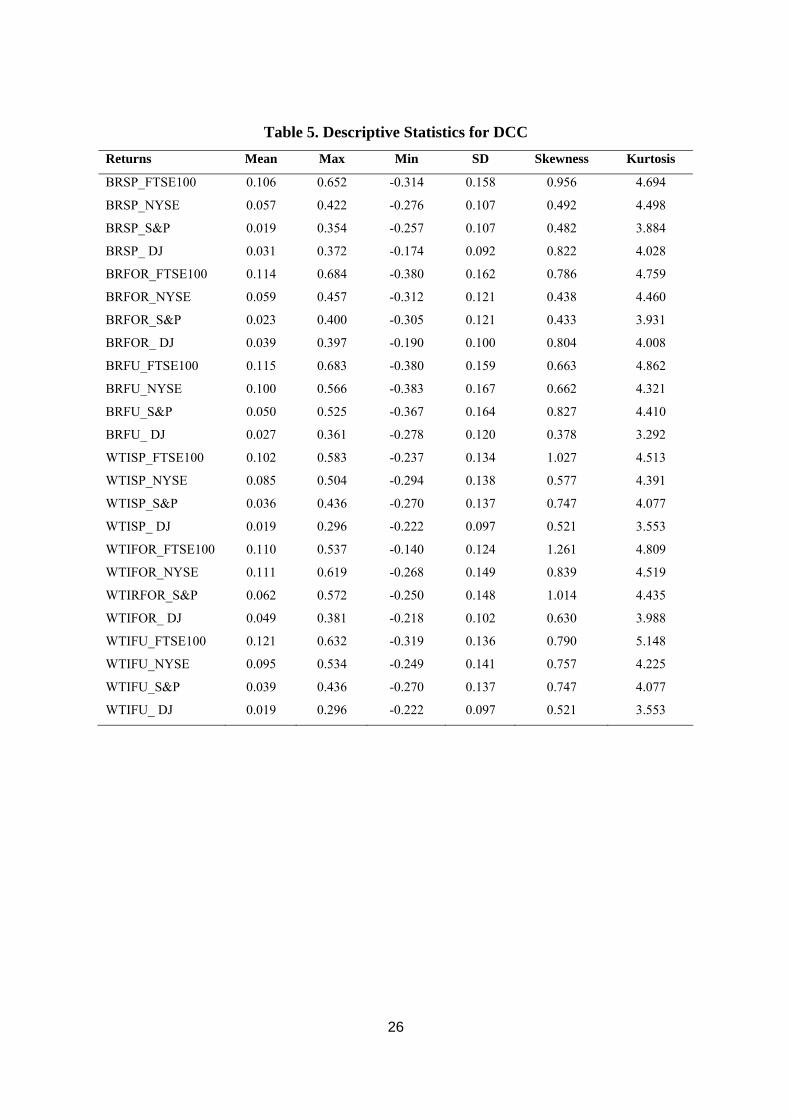
Table 5. Descriptive Statistics for DCC Returns Mean Max Min SD Skewness Kurtosis
BRSP_FTSE100 0.106 0.652 -0.314 0.158 0.956 4.694
BRSP_NYSE 0.057 0.422 -0.276 0.107 0.492 4.498
BRSP_S&P 0.019 0.354 -0.257 0.107 0.482 3.884
BRSP_ DJ 0.031 0.372 -0.174 0.092 0.822 4.028
BRFOR_FTSE100 0.114 0.684 -0.380 0.162 0.786 4.759
BRFOR_NYSE 0.059 0.457 -0.312 0.121 0.438 4.460
BRFOR_S&P 0.023 0.400 -0.305 0.121 0.433 3.931
BRFOR_ DJ 0.039 0.397 -0.190 0.100 0.804 4.008
BRFU_FTSE100 0.115 0.683 -0.380 0.159 0.663 4.862
BRFU_NYSE 0.100 0.566 -0.383 0.167 0.662 4.321
BRFU_S&P 0.050 0.525 -0.367 0.164 0.827 4.410
BRFU_ DJ 0.027 0.361 -0.278 0.120 0.378 3.292
WTISP_FTSE100 0.102 0.583 -0.237 0.134 1.027 4.513
WTISP_NYSE 0.085 0.504 -0.294 0.138 0.577 4.391
WTISP_S&P 0.036 0.436 -0.270 0.137 0.747 4.077
WTISP_ DJ 0.019 0.296 -0.222 0.097 0.521 3.553
WTIFOR_FTSE100 0.110 0.537 -0.140 0.124 1.261 4.809
WTIFOR_NYSE 0.111 0.619 -0.268 0.149 0.839 4.519
WTIRFOR_S&P 0.062 0.572 -0.250 0.148 1.014 4.435
WTIFOR_ DJ 0.049 0.381 -0.218 0.102 0.630 3.988
WTIFU_FTSE100 0.121 0.632 -0.319 0.136 0.790 5.148
WTIFU_NYSE 0.095 0.534 -0.249 0.141 0.757 4.225
WTIFU_S&P 0.039 0.436 -0.270 0.137 0.747 4.077
WTIFU_ DJ 0.019 0.296 -0.222 0.097 0.521 3.553
26
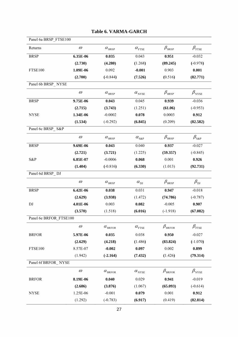
Table 6. VARMA-GARCH Panel 6a BRSP_FTSE100
Returns ω BRSPα FTSEα BRSPβ FTSEβ
BRSP 6.35E-06
(2.730)
0.035
(4.280)
0.043
(1.268)
0.951
(89.245)
-0.032
(-0.978)
FTSE100 1.09E-06
(2.700)
0.092
(-0.844)
-0.001
(7.526)
0.903
(0.516)
0.001
(82.771)
Panel 6b BRSP_ NYSE
ω BRSPα NYSEα BRSPβ NYSEβ
BRSP 9.75E-06
(2.715)
0.043
(3.743)
0.045
(1.251)
0.939
(61.06)
-0.036
(-0.953)
NYSE 1.34E-06
(1.534)
-0.0002
(-0.292)
0.078
(6.845)
0.0003
(0.209)
0.912
(82.582)
Panel 6c BRSP_ S&P
ω BRSPα S&Pα BRSPβ S&Pβ
BRSP 9.69E-06
(2.721)
0.043
(3.721)
0.040
(1.225)
0.937
(59.357)
-0.027
(-0.845)
S&P 6.85E-07
(1.404)
-0.0006
(-0.816)
0.068
(6.330)
0.001
(1.013)
0.926
(92.731)
Panel 6d BRSP_ DJ
ω BRSPα DJα BRSPβ DJβ
BRSP 6.42E-06
(2.629)
0.038
(3.938)
0.031
(1.472)
0.947
(74.786)
-0.018
(-0.787)
DJ 4.01E-06
(3.570)
0.003
(1.518)
0.082
(6.016)
-0.005
(-1.918)
0.907
(67.082)
Panel 6e BRFOR_FTSE100
ω BRFORα FTSEα BRFORβ FTSEβ
BRFOR 5.97E-06
(2.629)
0.035
(4.218)
0.038
(1.486)
0.950
(83.824)
-0.027
(-1.070)
FTSE100 8.57E-07
(1.942)
-0.002
(-2.164)
0.097
(7.432)
0.002
(1.426)
0.899
(79.314)
Panel 6f BRFOR_ NYSE
ω BRFORα NYSEα BRFORβ NYSEβ
BRFOR 8.19E-06
(2.686)
0.040
(3.876)
0.029
(1.067)
0.941
(65.093)
-0.019
(-0.614)
NYSE 1.25E-06
(1.292)
-0.001
(-0.783)
0.079
(6.917)
0.001
(0.419)
0.912
(82.814)
27
Panel 6g BRFOR_ S&P
ω BRFORα S&Pα BRFORβ S&Pβ
BRFOR 1.15E-05
(2.491)
0.046
(3.685)
0.028
(1.056)
0.925
(44.560)
-0.010
(-0.359)
S&P 6.73E-07
(1.235)
-0.001
(-0.773)
0.069
(6.378)
0.002
(0.852)
0.925
(91.513)
Panel 6h BRFOR_ DJ
ω BRFORα DJα BRFORβ DJβ
BRFOR 7.48E-06
(2.552)
0.040
(3.911)
0.023
(1.372)
0.938
(59.906)
-0.008
(-0.405)
DJ 3.39E-06
(2.624)
0.005
(1.275)
0.081
(5.900)
-0.004
(-1.0642)
0.905
(61.338)
Panel 6i BRFU_FTSE100
ω BRFUα FTSEα BRFUβ FTSEβ
BRFU 9.22E-06
(2.781)
0.045
(4.337)
0.050
(1.931)
0.936
(62.816)
-0.041
(-1.666)
FTSE100 7.36E-07
(1.717)
-0.002
(-1.930)
0.099
(7.490)
0.003
(1.579)
0.897
(77.307)
Panel 6j BRFU_ NYSE
ω BRFUα NYSEα BRFUβ NYSEβ
BRFU 1.09E-05
(2.845)
0.048
(3.982)
0.046
(1.535)
0.930
(52.592)
-0.035
(-1.087)
NYSE 9.81E-07
(1.451)
-0.001
(-0.562)
0.079
(6.931)
0.002
(0.787)
0.911
(79.700)
Panel 6k BRFU_ S&P
ω BRFUα S&Pα BRFUβ S&Pβ
BRFU 1.07E-05
(2.818)
0.048
(3.973)
0.040
(1.487)
0.928
(51.084)
-0.024
(-0.851)
S&P 2.11E-07
(1.514)
-0.002
(-1.048)
0.070
(6.597)
0.003
(1.296)
0.924
(85.800)
Panel 6l BRFU_ DJ
ω BRFUα DJα BRFUβ DJβ
BRFU 7.62E-06
(2.756)
0.044
(4.121)
0.027
(1.560)
0.935
(63.100)
-0.010
(-0.512)
DJ 3.20E-06
(2.764)
0.006
(1.848)
0.080
(5.845)
-0.005
(-1.393)
0.904
(58.532)
28
Panel 6m WTISP _FTSE100
ω WTISPα FTSEα WTISPβ FTSEβ
WTISP 4.29E-07
(0.862)
0.098
(7.392)
-0.001
(-0.721)
0.896
(77.035)
0.002
(1.267)
FTSE100 1.30E-05
(2.724)
0.054
(1.253)
0.049
(3.905)
-0.039
(-0.968)
0.928
(52.795)
Panel 6n WTISP_ NYSE
ω WTISPα NYSEα WTISPβ NYSEβ
WTISP 7.11E-07
(1.163)
0.079
(6.992)
-0.001
(-0.757)
0.9115
(80.704)
0.002
(1.288)
NYSE 1.61E-05
(2.715)
0.059
(1.235)
0.052
(3.601)
-0.039
(-0.753)
0.9194
(42.657)
Panel 6o WTISP_ S&P
ω WTISPα S&Pα WTISPβ S&Pβ
WTISP 2.57E-08
(0.099)
0.068
(6.554)
-0.001
(-0.961)
0.925
(89.934)
0.003
(1.505)
S&P 1.63E-05
(2.689)
0.0578
(1.384)
0.053
(3.578)
-0.029
(-0.661)
0.916
(39.664)
Panel 6p WTISP_DJ
ω WTISPα DJα WTISPβ DJβ
WTISP 9.58E-06
(2.276)
0.048
(3.673)
0.018
(0.768)
0.926
(50.138)
0.017
(0.596)
DJ 2.51E-06
(2.133)
0.0004
(0.220)
0.083
(5.845)
0.001
(0.390)
0.904
(58.177)
Panel 6q WTIFOR_FTSE100
ω WTIFORα FTSEα WTIFORβ FTSEβ
WTIFOR 4.90E-07
(1.024)
0.098
(7.623)
-0.002
(-2.655)
0.897
(81.742)
0.003
(2.035)
FTSE100 1.28E-05
(2.729)
0.045701
(1.411)
0.056
(4.268)
-0.023
(-0.690)
0.918
(48.917)
Panel 6r WTIFOR_ NYSE
ω WTIFORα NYSEα WTIFORβ NYSEβ
WTIFOR 7.12E-07
(1.479)
0.079
(6.767)
-0.002
(-1.916)
0.910
(83.173)
0.003
(1.515)
NYSE 1.56E-05
(2.825)
0.058
(1.022)
0.036
(4.047)
0.910
(-0.189)
-0.009
(41.583)
29
Panel 6s WTIFOR_S&P
ω WTIFORα S&Pα WTIFORβ S&Pβ
WTIFOR 8.98E-08
(0.663)
0.069
(6.610)
-0.002
(-1.441)
0.924
(88.676)
0.003
(1.738)
S&P 1.55E-05
(2.797)
0.032
(1.009)
0.059
(4.009)
0.002
(0.067)
0.907
(39.771)
Panel 6t WTIFOR_DJ
ω WTIFORα DJα WTIFORβ DJβ
WTIFOR 1.03E-05
(2.461)
0.055
(4.326)
0.007
(0.464)
0.917
(49.988)
0.024
(1.041)
DJ 3.05E-06
(2.565)
0.003
(0.987)
0.082
(5.827)
-0.002
(-0.497)
0.904
(58.398)
Panel 6u WTIFU_FTSE100
ω WTIFUα FTSEα WTIFUβ FTSEβ
WTIFU 1.48E-05
(2.980)
0.056
(4.009)
0.072
(1.618)
0.915
(46.339)
-0.0501
(-1.240)
FTSE100 3.91E-07
(0.828)
-0.002
(-2.259)
0.097
(7.384)
0.003
(2.046)
0.898
(78.023)
Panel 6v WTIFU_FTSE100
ω WTIFUα NYSEα WTIFUβ NYSEβ
WTIFU 1.91E-05
(3.063)
0.061
(3.740)
0.065
(1.231)
0.902
(37.690)
-0.037
(-0.681)
NYSE 4.01E-07
(0.784)
-0.001
(-1.357)
0.079
(6.740)
0.003
(1.343)
0.910
(82.999)
Panel 6w WTIFU_ S&P
ω WTIFUα S&Pα WTIFUβ S&Pβ
WTIFU 1.87E-05
(3.031)
0.062
(3.711)
0.054
(1.174)
0.899
(36.014)
-0.018
(-0.403)
S&P -2.35E-07
(-1.613)
-0.001
(-1.115)
0.068
(6.513)
0.004
(1.857)
0.925
(89.724)
Panel 6x WTIFU_ DJ
ω WTIFUα DJα WTIFUβ DJβ
WTIFU 1.27E-05
(2.731)
0.060
(3.754)
0.012
(0.612)
0.907
(40.670)
0.022
(0.856)
DJ 2.78E-06
(2.158)
0.002
(0.936)
0.081
(5.825)
-0.001
(-0.225)
0.904
(58.051)
30
Notes: The two entries for each parameter are their respective parameter estimates and Bollerslev and Wooldridge (1992) robust t- ratios. Entries in bold are significant at the 5% level.

31
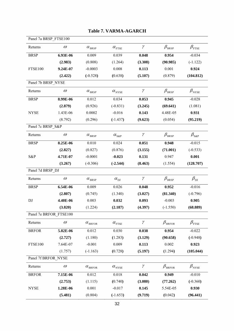
Table 7. VARMA-AGARCH Panel 7a BRSP_FTSE100
Returns ω BRSPα FTSEα γ BRSPβ FTSEβ
BRSP 6.93E-06
(2.983)
0.009
(0.808)
0.039
(1.264)
0.048
(3.308)
0.954
(90.985)
-0.034
(-1.122)
FTSE100 9.24E-07
(2.422)
-0.0003
(-0.528)
0.008
(0.638)
0.113
(5.107)
0.001
(0.879)
0.924
(104.812)
Panel 7b BRSP_NYSE
Returns ω BRSPα NYSEα γ BRSPβ NYSEβ
BRSP 8.99E-06
(2.879)
0.012
(0.926)
0.034
(-0.831)
0.053
(3.245)
0.945
(69.641)
-0.028
(1.081)
NYSE 1.43E-06
(8.792)
0.0002
(0.296)
-0.016
(-1.437)
0.143
(9.623)
4.48E-05
(0.054)
0.931
(95.219)
Panel 7c BRSP_S&P
Returns ω BRSPα S&Pα γ BRSPβ S&Pβ
BRSP 8.25E-06
(2.827)
0.010
(0.827)
0.024
(0.876)
0.051
(3.155)
0.948
(71.001)
-0.015
(-0.533)
S&P 4.71E-07
(3.267)
-0.0001
(-0.306)
-0.023
(-2.544)
0.131
(8.463)
0.947
(1.554)
0.001
(128.707)
Panel 7d BRSP_DJ
Returns ω BRSPα DJα γ BRSPβ DJβ
BRSP 6.54E-06
(2.807)
0.009
(0.745)
0.026
(1.340)
0.048
(3.027)
0.952
(81.340)
-0.016
(-0.796)
DJ 4.40E-06
(3.820)
0.003
(1.224)
0.032
(2.187)
0.093
(4.397)
-0.003
(-1.550)
0.905
(68.889)
Panel 7e BRFOR_FTSE100
Returns ω BRFORα FTSEα γ BRFORβ FTSEβ
BRFOR 5.82E-06
(2.727)
0.012
(1.180)
0.030
(1.283)
0.038
(3.129)
0.954
(90.658)
-0.022
(-0.948)
FTSE100 7.64E-07
(1.757)
-0.001
(-1.163)
0.009
(0.728)
0.113
(5.197)
0.002
(1.294)
0.923
(105.044)
Panel 7f BRFOR_NYSE
Returns ω BRFORα NYSEα γ BRFORβ NYSEβ
BRFOR 7.15E-06
(2.753)
0.012
(1.115)
0.018
(0.740)
0.042
(3.080)
0.949
(77.262)
-0.010
(-0.360)
NYSE 1.28E-06
(5.481)
0.001
(0.804)
-0.017
(-1.653)
0.145
(9.719)
5.54E-05
(0.042)
0.930
(96.441)
32
Panel 7g BRFOR_S&P
Returns ω BRFORα S&Pα γ BRFORβ S&Pβ
BRFOR 7.08E-06
(2.733)
0.012
(1.087)
0.014
(0.659)
0.043
(3.116)
0.9489
(74.963)
-0.004
(-0.185)
S&P 2.63E-07
(1.926)
0.0001
(0.223)
-0.025
(-2.790)
0.134
(8.504)
0.002
(1.594)
0.947
(126.729)
Panel 7h BRFOR_DJ
Returns ω BRFORα DJα γ BRFORβ DJβ
BRFOR 5.75E-06
(2.581)
0.012
(1.027)
0.014
(0.939)
0.041
(3.009)
0.951
(77.268)
-0.002
(-0.131)
DJ 3.13E-06
(2.384)
0.003
(0.797)
0.029
(2.053)
0.096
(4.546)
0.0001
(0.035)
0.902
(64.402)
Panel 7i BRFU_FTSE100
Returns ω BRFUα FTSEα γ BRFUβ FTSEβ
BRFU 7.60E-06
(3.094)
0.026
(2.125)
0.045
(1.828)
0.024
(1.761)
0.946
(79.696)
-0.040
(-1.686)
FTSE100 7.55E-07
(1.861)
-0.001
(-0.889)
0.009
(0.715)
0.114
(5.105)
0.002
(1.2720)
0.922
(102.996)
Panel 7j BRFU_NYSE
Returns ω BRFUα NYSEα γ BRFUβ NYSEβ
BRFU 1.03E-05
(2.925)
0.032
(2.271)
0.041
(1.431)
0.024
(1.594)
0.935
(56.689)
-0.034
(-1.100)
NYSE 1.04E-06
(4.003)
0.0004
(0.415)
-0.018
(-1.763)
0.145
(9.760)
0.001
(0.555)
0.930
(96.629)
Panel 7k BRFU_S&P
Returns ω BRFUα S&Pα γ BRFUβ S&Pβ
BRFU 1.02E-05
(2.886)
0.033
(2.275)
0.035
(1.365)
0.023
(1.554)
0.933
(54.556)
-0.023
(-0.848)
S&P 1.12E-07
(0.932)
-4.81E-05
(-0.048)
-0.024
(-2.713)
0.133
(8.304)
0.002
(1.633)
0.947
(126.27)
Panel 7l BRFU_DJ
Returns ω BRFUα DJα γ BRFUβ DJβ
BRFU 7.39E-06
(2.852)
0.027
(1.916)
0.026
(1.523)
0.025
(1.756)
0.941
(64.493)
-0.011
(-0.553)
Dow Jones 3.26E-06
(2.730)
0.005
(1.462)
0.028
(1.906)
0.097
(4.516)
-0.001
(-0.356)
0.900
(60.504)
33
Panel 7m WTISP_FTSE100
Returns ω WTISPα FTSEα γ WTISPβ FTSEβ
WTISP 1.41E-05
(3.098)
0.028
(2.046)
0.054
(1.270)
0.055
(2.130)
0.929
(56.98)
-0.042
(-1.043)
FTSE100 5.65E-07
(1.265)
-0.001
(-0.774)
0.008
(0.677)
0.115
(5.262)
0.002
(1.287)
0.921
(103.8)
Panel 7n WTISP_NYSE
Returns ω WTISPα NYSEα γ WTISPβ NYSEβ
WTISP 1.77E-05
(3.090)
0.030
(1.995)
0.061
(1.268)
0.040
(2.150)
0.918
(45.855)
-0.042
(-0.822)
NYSE 9.55E-07
(2.426)
-0.0002
(-0.287)
-0.016
(-1.397)
0.141
(9.228)
0.001
(0.826)
0.930
(98.293)
Panel 7o WTISP_S&P
Returns ω WTISPα S&Pα γ WTISPβ S&Pβ
WTISP 1.87E-05
(3.083)
0.032
(2.025)
0.059
(1.380)
0.042
(2.144)
0.910
(41.070)
-0.028
(-0.648)
S&P 2.15E-07
(1.831)
-0.0002
(-0.270)
-0.022
(-2.626)
0.129
(8.421)
0.002
(1.701)
0.947
(128.314)
Panel 7p WTISP_DJ
Returns ω WTISPα DJα γ WTISPβ DJβ
WTISP 1.11E-05
(2.564)
0.030
(1.915)
0.013
(0.585)
0.034
(1.872)
0.924
(49.662)
0.021
(0.760)
DJ 2.89E-06
(2.406)
-0.001
(-0.273)
0.029
(1.975)
0.098
(4.641)
0.003
(1.004)
0.901
(61.523)
Panel 7q WTIFOR_FTSE100
Returns ω WTIFORα FTSEα γ WTIFORβ FTSEβ
WTIFOR 1.14E-05
(3.040)
0.016
(1.470)
0.042
(1.432)
0.054
(3.185)
0.933
(65.867)
-0.026
(-0.879)
FTSE100 5.90E-07
(1.411)
-0.001
(-1.406)
0.009
(0.746)
0.113
(5.223)
0.003
(1.716)
0.922
(105.695)
Panel 7r WTIFOR_NYSE
Returns ω WTIFORα NYSEα γ WTIFORβ NYSEβ
WTIFOR 1.32E-05
(3.072)
0.017
(1.456)
0.030
(0.957)
0.055
(3.080)
0.927
(57.179)
-0.011
(-0.295)
NYSE 2.16E-06
(3.641)
-0.002
(-1.668)
-0.001
(-0.079)
0.157
(7.436)
0.005
(2.585)
0.889
(39.429)
34
Panel 7s WTIFOR_S&P
Returns ω WTIFORα S&Pα γ WTIFORβ S&Pβ
WTIFOR 1.32E-05
(3.030)
0.018
(1.459)
0.024
(0.866)
0.056
(3.077)
0.925
(53.997)
0.001
(0.033)
S&P 6.75E-07
(2.014)
-0.002
(-1.240)
-0.018
(-1.460)
0.152
(8.205)
0.005
(69.422)
0.924
(2.679)
Panel 7t WTIFOR_DJ
Returns ω WTIFORα DJα γ WTIFORβ DJβ
WTIFOR 9.20E-06
(2.730)
0.015260
(1.377671)
0.007
(0.453)
0.053
(3.149)
0.933
(67.590)
0.016
(0.780)
DJ 3.06E-06
(2.579)
0.001
(0.275)
0.029
(1.984)
0.098
(4.597)
0.002
(0.617)
0.901
(60.798)
Panel 7u WTIFU_FTSE100
Returns ω WTIFUα FTSEα γ WTIFUβ FTSEβ
WTIFU 1.40E-05
(3.360)
0.023
(1.599)
0.073
(1.674)
0.050
(3.017)
0.925
(56.133)
-0.056
(-1.421)
FTSE100 5.25E-07
(1.226)
-0.001
(-1.399)
0.009
(0.747)
0.113
(5.076)
0.003
(1.767)
0.922
(103.641)
Panel 7v WTIFU_NYSE
Returns ω WTIFUα NYSEα γ WTIFUβ NYSEβ
WTIFU 1.74E-05
(3.319)
0.026
(1.590)
0.065
(1.262)
0.053
(2.900)
0.914
(45.754)
-0.044
(-0.847)
NYSE 5.42E-07
(3.889)
-0.0003
(-0.421)
-0.017
(-1.607)
0.143
(9.588)
0.002
(1.913)
0.930
(96.195)
Panel 7w WTIFU_S&P
Returns ω WTIFUα S&Pα γ WTIFUβ S&Pβ
WTIFU 1.73E-05
(3.265)
0.028
(1.612)
0.053
(1.177)
0.053
(2.842)
0.909
(42.314)
-0.024
(-0.554)
S&P -8.61E-08
(-0.882)
-0.0001
(-0.195)
-0.025
(-2.874)
0.131
(8.4171)
0.003
(2.386)
0.948
(132.341)
Panel 7x WTIFU_DJ
Returns ω WTIFUα DJα γ WTIFUβ DJβ
WTIFU 1.25E-05
(2.926)
0.029
(1.558)
0.009
(0.461)
0.049
(2.627)
0.914
(43.890)
0.022
(0.886)
DJ 2.88E-06
(2.259)
0.001
(0.353)
0.029
(1.968)
0.097
(4.603)
0.002
(0.619)
0.901
(61.100)
35
Notes: The two entries for each parameter are their respective parameter estimates and Bollerslev and Wooldridge (1992) robust t-ratios. Entries in bold are significant at the 5% level

36
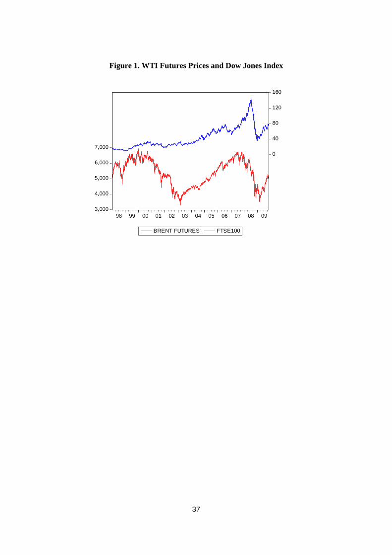
Figure 1. WTI Futures Prices and Dow Jones Index
3,000
4,000
5,000
6,000
7,0000
40
80
120
160
98 99 00 01 02 03 04 05 06 07 08 09
BRENT FUTURES FTSE100
37
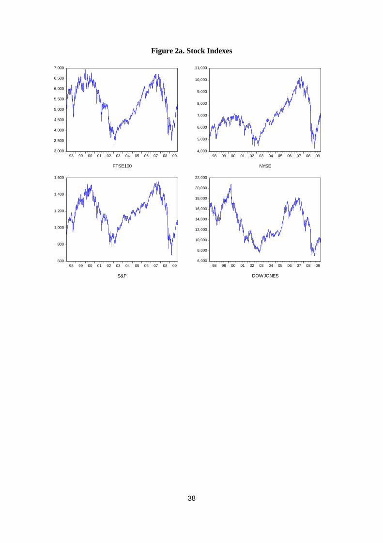
Figure 2a. Stock Indexes
6,000
8,000
10,000
12,000
14,000
16,000
18,000
20,000
22,000
98 99 00 01 02 03 04 05 06 07 08 09
DOWJONES
3,000
3,500
4,000
4,500
5,000
5,500
6,000
6,500
7,000
98 99 00 01 02 03 04 05 06 07 08 09
FTSE100
600
800
1,000
1,200
1,400
1,600
98 99 00 01 02 03 04 05 06 07 08 09
S&P
4,000
5,000
6,000
7,000
8,000
9,000
10,000
11,000
98 99 00 01 02 03 04 05 06 07 08 09
NYSE
38
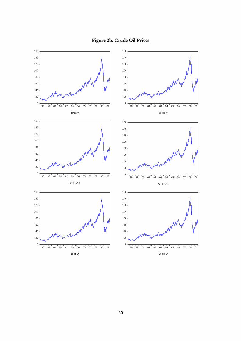
Figure 2b. Crude Oil Prices
0
20
40
60
80
100
120
140
160
98 99 00 01 02 03 04 05 06 07 08 09
BRSP
0
20
40
60
80
100
120
140
160
98 99 00 01 02 03 04 05 06 07 08 09
WTISP
0
20
40
60
80
100
120
140
160
98 99 00 01 02 03 04 05 06 07 08 09
BRFOR
0
20
40
60
80
100
120
140
160
98 99 00 01 02 03 04 05 06 07 08 09
WTIFOR
0
20
40
60
80
100
120
140
160
98 99 00 01 02 03 04 05 06 07 08 09
BRFU
0
20
40
60
80
100
120
140
160
98 99 00 01 02 03 04 05 06 07 08 09
WTIFU
39
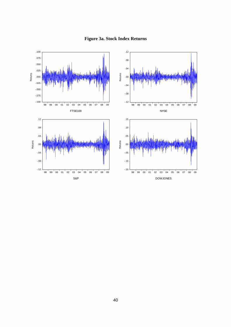
Figure 3a. Stock Index Returns
-.15
-.10
-.05
.00
.05
.10
.15
98 99 00 01 02 03 04 05 06 07 08 09
DOWJONES
Ret
urns
-.100
-.075
-.050
-.025
.000
.025
.050
.075
.100
98 99 00 01 02 03 04 05 06 07 08 09
FTSE100
Ret
urns
-.12
-.08
-.04
.00
.04
.08
.12
98 99 00 01 02 03 04 05 06 07 08 09
NYSE
Ret
urns
-.12
-.08
-.04
.00
.04
.08
.12
98 99 00 01 02 03 04 05 06 07 08 09
S&P
Ret
urns
40
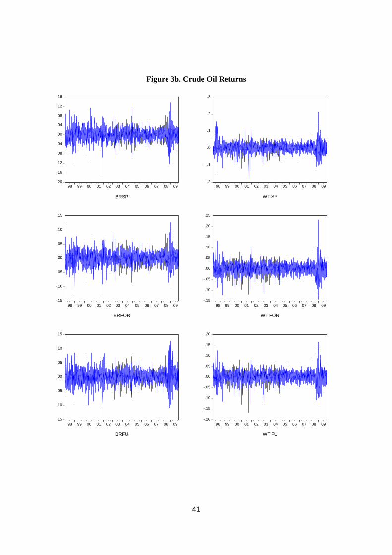
Figure 3b. Crude Oil Returns
-.20
-.16
-.12
-.08
-.04
.00
.04
.08
.12
.16
98 99 00 01 02 03 04 05 06 07 08 09
BRSP
-.2
-.1
.0
.1
.2
.3
98 99 00 01 02 03 04 05 06 07 08 09
WTISP
-.15
-.10
-.05
.00
.05
.10
.15
98 99 00 01 02 03 04 05 06 07 08 09
BRFOR
-.15
-.10
-.05
.00
.05
.10
.15
.20
.25
98 99 00 01 02 03 04 05 06 07 08 09
WTIFOR
-.15
-.10
-.05
.00
.05
.10
.15
98 99 00 01 02 03 04 05 06 07 08 09
BRFU
-.20
-.15
-.10
-.05
.00
.05
.10
.15
.20
98 99 00 01 02 03 04 05 06 07 08 09
WTIFU
41
42
Figure 4. Dynamic Conditional Correlations
-.4
-.2
.0
.2
.4
.6
-.4
-.2
.0
.2
.4
.6
.8
98 99 00 01 02 03 04 05 06 07 08 09
BRSP_FTSE BRSP_NYSE
-.4
-.2
.0
.2
.4
.6
-.4
-.2
.0
.2
.4
.6
.8
98 99 00 01 02 03 04 05 06 07 08 09
BRFOR_FTSE BRFOR_NYSE
-.4
-.2
.0
.2
.4
.6
-.2
.0
.2
.4
.6
98 99 00 01 02 03 04 05 06 07 08 09
BRFOR_DJ BRFOR_S&P
-.4
-.2
.0
.2
.4
.6
-.4
-.2
.0
.2
.4
98 99 00 01 02 03 04 05 06 07 08 09
BRFU_DJ BRFU_S&P
-.4
-.2
.0
.2
.4
.6
-.4
-.2
.0
.2
.4
.6
.8
98 99 00 01 02 03 04 05 06 07 08 09
BRFU_FTSE BRFU_NYSE
-.2
-.1
.0
.1
.2
.3
.4
-.4
-.2
.0
.2
.4
98 99 00 01 02 03 04 05 06 07 08 09
BRSP_DJ BRSP_S&P
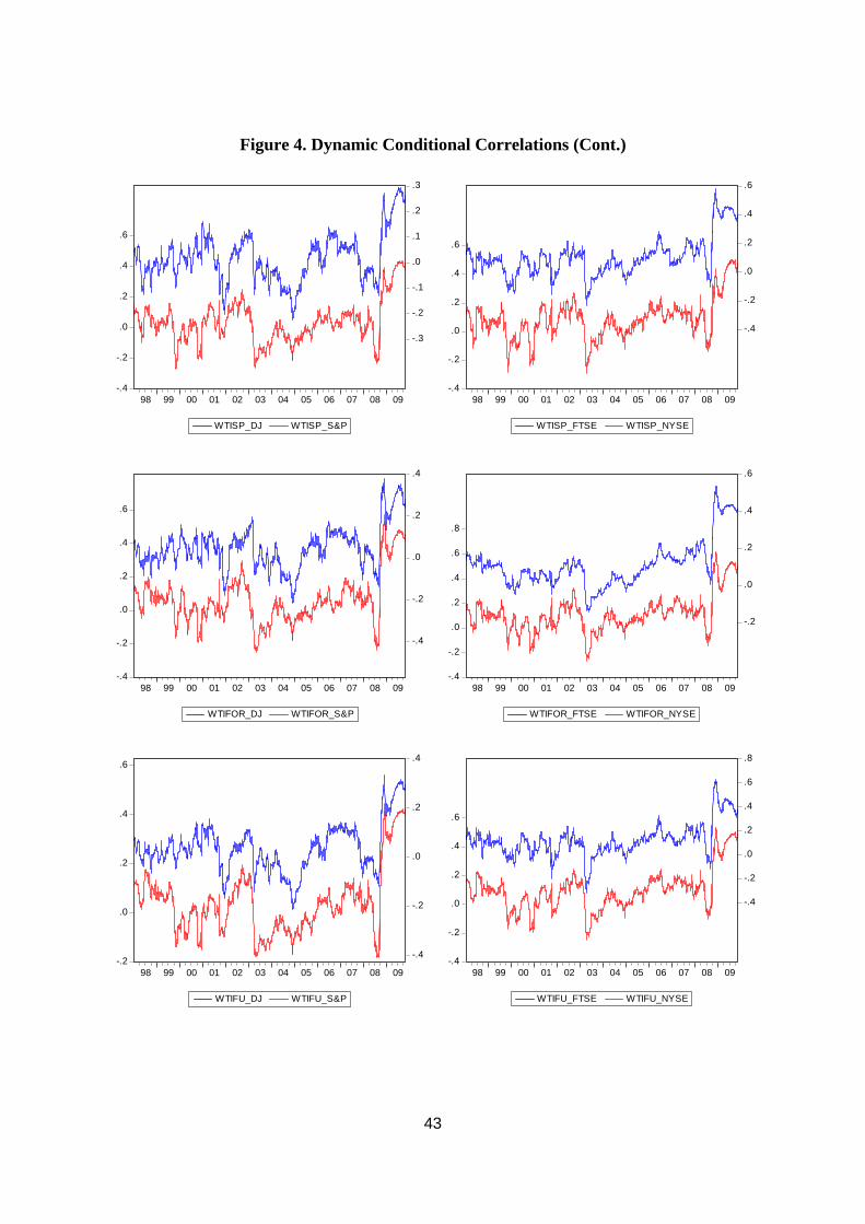
Figure 4. Dynamic Conditional Correlations (Cont.)
-.4
-.2
.0
.2
.4
.6
-.3
-.2
-.1
.0
.1
.2
.3
98 99 00 01 02 03 04 05 06 07 08 09
WTISP_DJ WTISP_S&P
-.4
-.2
.0
.2
.4
.6
-.4
-.2
.0
.2
.4
.6
98 99 00 01 02 03 04 05 06 07 08 09
WTISP_FTSE WTISP_NYSE
-.4
-.2
.0
.2
.4
.6
-.4
-.2
.0
.2
.4
98 99 00 01 02 03 04 05 06 07 08 09
WTIFOR_DJ WTIFOR_S&P
-.4
-.2
.0
.2
.4
.6
.8
-.2
.0
.2
.4
.6
98 99 00 01 02 03 04 05 06 07 08 09
WTIFOR_FTSE WTIFOR_NYSE
-.2
.0
.2
.4
.6
-.4
-.2
.0
.2
.4
98 99 00 01 02 03 04 05 06 07 08 09
WTIFU_DJ WTIFU_S&P
-.4
-.2
.0
.2
.4
.6
-.4
-.2
.0
.2
.4
.6
.8
98 99 00 01 02 03 04 05 06 07 08 09
WTIFU_FTSE WTIFU_NYSE
43