Embed Size (px)
Citation preview

Discussion Paper No. 686
“A Dynamic Two Country Heckscher-Ohlin Model with Non-Homothetic Preferences”
Eric W. Bond, Kazumichi Iwasa and Kazuo Nishimura
November 2009
KYOTO UNIVERSITY
KYOTO, JAPAN
KYOTO INSTITUTE OF
ECONOMIC RESEARCH
KIER DISCUSSION PAPER SERIES

A Dynamic Two Country Heckscher-Ohlin Model with Non-Homothetic Preferences
Eric W. Bond1, Kazumichi Iwasa2 and Kazuo Nishimura3
1Department of Economics, Vanderbilt University, VU Station B #351819, 2301 Vanderbilt Place,
Nashville, TN 37235-1819, USA
(e-mail: [email protected])2KIER, Kyoto University, Yoshida-Honmachi, Sakyo-ku, Kyoto 606-8501, Japan
(e-mail: [email protected])3KIER, Kyoto University, Yoshida-Honmachi, Sakyo-ku, Kyoto 606-8501, Japan
(e-mail: [email protected])
Summary. We examine the properties of a two country dynamic Heckscher-Ohlin model that
allows for preferences to be non-homothetic. We show that the model has a continuum of steady
state equilibria under free trade, with the initial conditions determining which equilibrium will be
attained. We establish conditions under which a static Heckscher-Ohlin theorem will hold in the
steady state, and also conditions for a dynamic H-O theorem to hold. If both goods are normal, each
country will have a unique autarkic steady state, and all steady state equilibria are saddle points.
We also consider the case in which one good is inferior, and show that this can lead to multiple
autarkic steady states, violations of the static H-O theorem in the steady state. Furthermore, there
may exist steady state equilibria that Pareto dominate other steady states. These steady states will
be unstable if discount factors are the same in each country, although they may exhibit dynamic
indeterminacy if discount factors di¤er.
Key words: two-country model, Heckscher-Ohlin, inferior good, multiple equilibria, indeterminacy
JEL Classi�cation Numbers: E13, E32, F11, F43
1

1 Introduction
In this paper we examine the role of tastes in determining the steady state capital stocks, the pattern
of trade and the local dynamic properties of steady state equilibria in a dynamic Heckscher-Ohlin
(H-O) model of international trade. It is well known that the predictions of the static H-O model
may be overturned if the tastes of a country are strongly biased toward the good that uses its
abundant factor intensively. The role of tastes is more complex in a dynamic model, because they
can a¤ect both the allocation of spending at a point in time as well as the intertemporal allocation
of spending.
The static model with identical and homothetic preferences generates demands for goods that
are independent of the international distribution of income. The analog of this assumption in the
dynamic model, which makes demands for goods independent of the international distribution of
wealth, is to assume identical and homothetic preferences with a constant intertemporal elasticity of
substitution (CIES). Chen [10] examined the dynamic H-O model with preferences of that type and
showed that it yields a continuum of steady state equilibria under free trade, with the world capital
stock being constant across all of the steady states. Which steady state the world economy converges
to is determined by the initial distribution of capital across countries because a country�s wealth
a¤ects its savings behavior. Initial di¤erences in wealth will thus have persistent e¤ects on capital
accumulation and will determine steady state capital stocks. Chen also showed that the pattern
of trade in the steady state will be determined by relative factor supplies, and is thus consistent
with the predictions of the static H-O theorem. Ventura [25] has utilized a similar model, which
allows for the possibility of endogenous growth as well as a steady state, to study the implications
of international trade for the convergence of per capita incomes across countries.1
Most of the existing literature on taste di¤erences has focused on di¤erences in rates of time
preference across countries. Stiglitz [24] analyzed the case with in�nitely lived consumers and showed
that the patient country will export the capital intensive good in the steady state. The assumption
of di¤erent rates of time preference means that countries will have di¤erent autarkic steady states,
and that at least one country will specialize in production in the steady state. Galor and Lin [13]
examine the e¤ect of di¤erences in time preference in an overlapping generations model, and also
obtain the result that the patient country will export the capital intensive good in the steady state.
They assume that the investment good be capital intensive in order to ensure a unique path to the
steady state.2
Our analysis will focus on the case of in�nitely lived consumers with identical preferences across
countries, but we relax the requirement that they be homothetic. We will also assume that the
1Bond et al [8] analyze a Heckscher-Ohlin model in which there is accumulation of both capital and labor (through
accumulation of human capital). They establish existence of a balanced growth path for the world economy, but show
that the accumulation paths of individual countries are indeterminate because households are indi¤erent between
physical and human capital accumulation at the margin.2Galor [12] shows that there will be indeterminacy if the consumption good is capital intensive.
2

sum of the rate of time preference and the depreciation rate is the same across countries, which
ensures that the autarkic steady state prices of the two goods are the same. This means that taste
di¤erences do not serve as a source of long run comparative advantage.
One goal of our analysis is to show how the non-homotheticity of tastes a¤ects the characteristics
of the steady state equilibria and the pattern of trade. We show that there will be a continuum
of steady states for the world economy in the general case, but the potential for non-homothetic
preferences alters the characteristics of the set of steady state equilibria. We �rst consider the case
in which all goods are normal, and show that the H-O theorem must hold as long as the discount
parameter is the same across countries. However, it can be violated if the discount factors are not
equal across countries. The world capital stock will not be constant across the potential steady
states because the distribution of world income a¤ects demands. We also consider the case in which
one of the goods is inferior, and show that this leads to the possibility that some steady states that
yield higher capital stocks for both countries than other steady states.
A second objective of our analysis is to analyze the implications of non-homotheticity in demand
for the dynamics of the international economy in the neighborhood of the steady state. We �rst
establish a su¢ cient condition for a steady state to be a saddle point, and show that this condition
is satis�ed as long as both goods are normal. We also show that the condition will be satis�ed when
one good is inferior for one of the countries as long as the e¤ect of inferiority is not too large. In
the case discount rates are the same across countries, the steady state equilibrium must be either a
source or a saddle point. However, there is a possibility of dynamic indeterminacy in the case where
discount rates di¤er across countries.
The possibility of dynamic indeterminacy in a two country trade model typically arises due to
the existence of a distortion in markets or due to market incompleteness. For example, Nishimura
and Shimomura [18] derived the possibility of local indeterminacy by introducing factor-generated
externalities into a dynamic two-country H-O model. Shimomura [23] and Doi et al. [11] showed
that indeterminacy can arise around one of the steady states in an endowment model of international
trade in which one of the goods is durable and there is a negative income e¤ect. Bond and Driskill
[9] showed that multiple steady states and indeterminacy can arise in the model with a durable good
when both goods are normal as long as the exporting country has the higher marginal propensity to
consume a good. The indeterminacy in the trade models with durable goods arises due to market
incompleteness due to the assumption that there is no international lending or borrowing. The same
market incompleteness arises in the H-O model of trade we examine. However, if there is factor
price equalization along the optimal path, international lending and borrowing is redundant if the
discount factors of the two countries are the same. As a result, a di¤erence in discount factors
between countries and inferiority in consumption are both necessary conditions for indeterminacy
to occur.
3

2 The Dynamic Two-Country Heckscher-Ohlin Model
In this section we formulate the continuous-time version dynamic optimization problem for a repre-
sentative country in a dynamic H-O model. By dynamic H-O model, we mean that each country has
access to the same technology for producing two goods using a �xed factor (labor) and a reproducible
factor (capital) under conditions of perfect competition and constant returns to scale. Good 1 is a
pure consumption good, and the second good is a consumable capital good. Factors of production
are assumed to be mobile between sectors within a country, but immobile internationally, and there
are no markets for international borrowing and lending. We refer to the representative country as
the home country: the corresponding behavioral relations for the other (foreign) country will be
denoted by a ��.�We assume that the home (foreign) country is made up of H (H�) households, with each house-
hold having an endowment of labor, l, and a concave utility function u de�ned over consumption
of goods 1 and 2, c1 and c2. The restriction that the labor endowment per household and the
household utility function are common across countries de�nes a sense in which each country has
the same preferences, although the household preferences are not necessarily homothetic. It also
means that we can distinguish between variations in the scale of the economy, which changes the
number of households but keeps wealth per household constant, and variations in the wealth of a
household. This distinction is useful in the case where preferences are not homothetic.
2.1 The Production Side
As to technologies, we will assume that
Assumption 1: The production function in each sector is quasi-concave and linearly homoge-neous. Pure consumption good 1 is labor intensive.
Letting w denote the wage rate and r the rental on capital, the technology in sector i can be
characterized by the unit cost function �i(w; r), i = 1; 2. The competitive pro�t conditions require
that
p � �1(w; r); (1)
1 � �2(w; r); (2)
where good 2 is chosen as numeraire. The aggregate stocks of labor and capital are denoted by L
and K respectively. Factor market equilibrium requires that
1 = v1 + v2; (3)
K=L = v1�1(w=r) + v2�2(w=r); (4)
4

where vi is the fraction of labor devoted to sector i and �i(w=r) = �ir(w; r)=�iw(w; r).
Solving for w and r when (1) and (2) hold with equality, we obtain the factor prices (w(p); r(p))
that are consistent with production of both goods. These factor prices will satisfy full employment
for K=L 2 [�1(w=r); �2(w=r)]. We will make assumptions below regarding tastes and discount
factors and depreciation rates that will ensure that any steady state equilibrium must involve a
price consistent with incomplete specialization in each country. Since our analysis will focus on
properties of the steady state and the behavior in the neighborhood of the steady state, we will limit
our presentation of the production side to the case of incomplete specialization.
With incomplete specialization, we can express GNP as w(p)L + r(p)K. Our assumption that
households have identical labor endowments implies that L = Hl. It will further be assumed that
the initial endowment of capital is equally distributed across households, so we can denote the initial
per household stock of capital by k0 = K0=H. This will imply identical holdings of capital across
households at each point in time, k = K=H, which makes it convenient to express the production
side on a per household basis. Applying the envelope theorem, we obtain the per household output
of good i, yi to be
y1(p; k; l) = w0(p)l + r0(p)k; y2(p; k; l) = w(p)l + r(p)k � p[w0(p)l + r0(p)k]: (5)
The supply functions are linear in k and l with incomplete specialization, where r0(p) < 0 since good
1 is labor intensive.
2.2 The Consumption Side
We analyze the optimization problem for a representative household that owns l units of labor under
the assumption that the initial endowment of capital of a household is k0 = K0=H. We will impose
the following restrictions on this utility function:
Assumption 2: The utility function is concave, with u11 < 0 and D � u11u22 � u12u21 > 0 forany (c1; c2) 2 f(c1; c2) 2 R2+jui(c1; c2) > 0, i = 1; 2g.
The representative household is assumed to maximize the discounted sum of its utilities
max
Z 1
0
u(c1; c2)e��tdt; (6)
subject to its �ow budget constraint
w(p)l + r(p)k = pc1 + c2 + _k + �k; k0 given, (7)
where � is the rate of depreciation on home country capital and � is the home country discount
rate. The budget constraint re�ects the assumed absence of an international capital market, since
5

it requires that pz1 + z2 = 0, where z1 = c1 � y1 (z2 = c2 + _k+ �k� y2) is the per household excessdemand for good 1 (2).
Solving the current value Hamiltonian for this problem yields the necessary conditions for the
choice of consumption levels, the di¤erential equation describing the evolution of the costate variable,
�, and the transversality conditions:
u1(c1; c2) = �p; u2(c1; c2) = �; (8)
_� = �[�+ � � r(p)]; (9)
limt!1
k(t)�(t)e��t = 0: (10)
It will be useful for the subsequent analysis to invert the necessary conditions for choice of
consumption levels to obtain consumption relations ci(p; �) for i = 1; 2 and an expenditure relation
E(p; �) � pc1(p; �) + c2(p; �). The following lemma, which is proven in the Appendix, establishes
some properties of these functions.
Lemma 1 (i) �c1� = pc1p + c2p. (ii) E� = pc1� + c2� < 0. (iii) c1p < 0. (iv) Ep = c1 + �c1�.
Our expenditure relation di¤ers from the standard expenditure function in that it holds constant
the marginal utility of income, rather than the level of utility. Good i is normal if ci� < 0, so
(ii) establishes that goods must be normal in total. For the case in which the utility function is
homothetic and has CIES of &, we have E(p; �) = e(p)��& .
Using (7), (9), and the expenditure function, we can express _k and _� as functions of (k; �; p) :
_k = w (p) l + r (p) k � E(p; �)� �k; (11)
_� = �[�+ � � r(p)]: (12)
In the case of autarky, the system is closed by adding the market clearing condition for good 1 at
home,
z1(p; k; l; �) � c1(p; �)� y1(p; k; l) = 0: (13)
Equations (11), (12), and (13) govern the evolution of (k; �; p) under autarky.
2.3 The Foreign Country and World Market Equilibrium
The optimization problem for a foreign household is analogous to that for the home country. The
technologies of the two countries are assumed to be the same, so w�(p) = w(p) and r�(p) = r(p)
for k�=l 2 [�1(w(p)=r(p)); �2(w(p)=r(p))]. Since household utility functions are the same across
6

countries, we have c�i (:) = ci(:) and E�(:) = E(:). Substituting these relations into the solution of
the foreign country�s household optimization problem yields
_k� = w (p�) l + r (p�) k� � E(p�; ��)� ��k� (14)
_�� = ��[�� + �� � r(p�)]: (15)
The foreign autarkic equilibrium can be described by (14), (15), and z1(p�; k�; l; ��) = 0.
In a free trade equilibrium, the price of good 1 will be equalized across countries and will be
determined by the world market clearing condition for good 1,
Hz1(p; k; l; �) +H�z1(p; k
�; l; ��) = 0: (16)
The free trade equilibrium can be solved for the evolution of (k; k�; �; ��; p) using (11), (12), (14),
(15), and (16). In our analysis of the free trade equilibrium, we will assume that
Assumption 3: � � �+ � = �� + ��; � � ��.
This condition ensures that _�=� = _��=�� at each point in time as long as the conditions for factor
price equalization are satis�ed. This will result in �� = m� for some m > 0 along the optimal
path, which simpli�es the analysis by reducing the dimensionality of the system. In the case where
� = ��, the solution to the competitive equilibrium will also be Pareto optimal because free trade
equates both the marginal rates of substitution between goods at a point and the marginal rate of
substitution between goods at di¤erent points in time in this case. Therefore, opening international
capital markets is unnecessary if discount factors are equal. This is the case in which all of the
technology and taste parameters are identical across countries, so that countries di¤er only in their
initial endowments of factors of production. If � > ��, the home country households are more
impatient and have less of a desire to accumulate capital, but the home country is a better location
to place capital (because � < ��), which implies that the real interest rate di¤ers across countries
under factor price equalization (r(p) � � > r(p) � ��). Without international capital markets,
therefore, this solution is not Pareto optimal. Indeed, there will exist additional gains from opening
international capital markets to allow foreign households to own capital located in the home country.
3 World Market Equilibrium
We begin our analysis of the world market equilibrium by deriving conditions for existence of a
steady state equilibrium price, and showing that this price is the only one consistent with a steady
state equilibrium under autarky or free trade. We then derive the steady state relationship between
the marginal utility of income and excess demand for good 1, which can be used to characterize the
steady state trade patterns and determine the conditions under which the Heckscher-Ohlin theorem
7

holds. We conclude by analyzing the dynamics of the world equilibrium in the neighborhood of the
steady state, and establishing conditions under which the initially capital abundant country remains
capital abundant along the path to the steady state.
We �rst establish su¢ cient conditions for existence and uniqueness of a steady state price at
which _k = _k� = _� = _�� = 0. Condition (12) requires that r = � in order to have _� = 0, and
Assumption 3 ensures that this will also yield _�� = 0. In order for this to be consistent with
incomplete specialization, the competitive pro�t conditions (1) and (2) must hold with equality
when r = �. So, we assume that3
Assumption 4: inffrj�2(w; r) = 1g < � < supfrj�2(w; r) = 1g.
Then, (2) can be inverted to obtain a unique steady state wage rate ~w(�) that is consistent with
competitive production of good 2. Competitive production of good 1 will require a price ~p(�) =
�1( ~w(�); �). This will be the only possible price consistent with a steady state when technologies are
the same in all countries, since there would be no production of good 1 (2) with r = � for p < ~p(�)
(p > ~p(�)). This steady state relative factor price, ~w(�)=�, will determine a unique capital labor ratio
employed in production in sector i in the steady state, �i( ~w(�)=�). Letting ~�min(�) � �1( ~w(�)=�)
and ~�max(�) � �2( ~w(�)=�), full employment will require that k=l; k�=l 2 [~�min(�); ~�max(�)].
Lemma 2 Let Assumption 4 hold. Then, there will exist a unique steady state wage, ~w(�), andprice, ~p(�), consistent with a steady state equilibrium with incomplete specialization.
The household budget constraint (11) requires that the per household steady state capital stock
satisfy4
~k(�; l; �) =E(~p; �)� ~wl
�; (17)
if _k = 0. Equation (17) illustrates a negative relationship between the steady state values of � and k.
Higher levels of the capital stock are associated with higher income and expenditure, which requires
a lower marginal utility of income. Since ~k�(�; l; �) < 0, we can invert (17) to de�ne a range of
feasible steady state values of �, �(l; �) = (~�min(l; �); ~�max(l; �)), where ~�min and ~�max are de�ned
as the solutions to ~k(�; l; �)=l = ~�max and ~k(�; l; �)=l = ~�min, respectively.5
3The right hand inequality would fail in the case of a �xed coe¢ cients production function in sector 2 where the
output per unit capital is less than �. In that case the productivity of capital is too low to justify replacement and the
existing stock of capital would be allowed to depreciate. The left hand inequality could fail if the marginal product of
capital in sector 2 has a lower bound exceeding �, as could arise with a CES production function where the elasticity
of substitution exceeds 1.4 In order to simplify the presentation, we suppress the dependence of steady state values on �, which is �xed, in
the following discussion.5 In the following, we suppress l and � as aruguments of ~�min and ~�max when there is no ambiguity.
8

Substituting (17) into the per household excess demand for good 1, we obtain a steady state (per
household) excess demand function
~z1(�; l; �) = c1(~p; �)� y1(~p; ~k(�; l; �); l): (18)
The autarkic steady state equilibrium is obtained by solving ~z1(�; l; �) = 0. Since good 1 is labor
intensive, y1(~p; ~k(~�min; l; �); l) = 0 and y1(~p; ~k(~�max; l; �); l) = [E(~p; ~�max) + �~k(~�max; l; �)]=~p. The
former implies that ~z1(~�min; l; �) = c1(~p; ~�min) > 0 and the latter that ~z1(~�max; l; �) = �[c2(~p; ~�max)+�~k(~�max; l; �)]=~p < 0, which ensures the existence of a steady state equilibrium.6
To establish conditions for the uniqueness of the autarkic steady state equilibrium, we di¤eren-
tiate (18) with respect to � and use (5) to obtain
~z1� = c1� �r0(~p)E��
; (19)
which is negative when good 1 is normal, since good 1 is labor intensive (r0 < 0). With the normality
in consumption, therefore, the equilibrium will be unique. In the rest of this section except for
subsection 3.2 on equilibrium dynamics, we will assume that
Assumption 5: Both goods are normal at all levels of income.
Figure 1 illustrates the steady state per household excess demand function. If � = ��, the foreign
excess demand function will coincide with that of the home country and the autarkic steady states
for the two countries will exhibit the same prices and the same marginal utility of income. To see
the e¤ect of di¤erences in the rate of time preference across countries (holding � + � constant), we
totally di¤erentiate ~z1(�; l; �) = 0 and to obtain
d�A
d�= �k
Ar0(~p)
�~z1�< 0;
@kA
@�= �k
Ac1��~z1�
< 0: (20)
Since both the numerator and denominator in the �rst expression are negative, an increase in the
discount factor will be associated with a higher steady state utility level in autarky. This result
can be understood by noting that (17) requires that ~k(�; l; �) is decreasing in �, because a given
expenditure level can be sustained with a lower capital stock. Referring to Figure 1, the decrease in~k(�; l; �) will shift ~z1 downward, resulting in a lower autarkic value of �.
6Ventura [25] utilizes a model in which there are two traded intermediate goods (one produced using labor only,
the other using capital only) that are combined to produce a non-traded �nal good. The �nal good can be either
consumed or used as a capital good, and preferences have a constant intertemporal elasticity of substitution. Although
the strucutre is slightly di¤erent from the one assumed here, it generates a steady state excess demand with properties
virtually identical to those derived here. Letting the �nal good be chosen as numeraire and assuming good 1 is the
labor intensive intermediate, we have E(1; �) = ��& and ~k(�; l; �) = (��& � ~wl)=�. Letting �(w; r) denote the unit
cost function for the �nal good, we have s1 = l and d1 = �w( ~w; �)��& , where s1 and d1 are the supply and demand
for intermediate good 1 (� = 0 is assumed), respectively.
9

The second result shows that if good 1 is normal, an increase in the discount factor will decrease
the steady state capital stock. Note that the increase in � has two e¤ects on the autarkic steady
state capital stock kA. One is a direct negative e¤ect due to @~k=@� < 0 and the other originates from
the decrease in �A (d�A=d� < 0), which is positive from @~k=@� < 0. The negative e¤ect dominates
the positive one.
These results can be summarized as
Proposition 1 :(a) There is unique autarkic steady state values (�A; kA) for the home countrysatisfying ~z1(�A; l; �) = 0 and kA = ~k(�A; l; �). The foreign country will have the same autarkic
steady state price as the home country.
(b) If � = ��, the home and foreign countries will have the same autarkic capital stocks and
utility levels. If � > ��, the home country will have a higher autarkic utility level than the foreign
country. The home capital stock will be lower.
3.1 Free Trade Steady States with Normal Goods
A steady state equilibrium with trade exists for any values of � and �� at which the world market
for good 1 clears,
Z(�; ��; l) � H~z1(�; l; �) +H�~z1(��; l; ��) = 0: (21)
It follows from Proposition 1 that (�A; �A�) is a solution to (21), and that these solutions are in
the interior of the respective regions. Since the excess demand functions are continuous, it follows
that there will be a continuum of pairs (�; ��) satisfying (21). If goods are normal, these pairs must
satisfy d��=d�jdZ=0 = �[H~z1�(�; l; �)]=[H�~z1�(��; l; ��)] < 0. Since there is a one to one relationship
between k and � from (17), the following Proposition holds.7
Proposition 2 : There is a continuum of per household capital stocks (k; k�) consistent with a
steady state equilibrium. These steady states can be described by a continuous function '(k) de�ned
on a non-empty interval, where the pair of per household capital stocks (k; '(k)) is a steady state
equilibrium and
'0(k) = � H
H�
24 ��~pc1�E�
� ~pr0(~p)�
����~pc�1�E��� ~pr0(~p)
��
�35 < 0: (22)
The world capital stock is the same across all of the steady states if preferences are homothetic and
� = ��. If the marginal propensity to consume good 1 is increasing (decreasing) in � and � = ��,
'00(k) > (<) 0.
7Hereafter, we attach �*� to the values of functions for foreign country when we omit their arguments, e.g. ~z�1�denotes ~z1�(��; l; ��).
10

When preferences are homothetic and � = �� (hence � = ��), the bracketed expression equals 1
and the world capital stock is constant in all of the trading equilibria. This is due to the fact that
a transfer of capital from one country to another has no e¤ect on world outputs as long as both
countries remain incompletely specialized. This transfer will also leave world demand una¤ected if
tastes are identical and homothetic and � = ��, so the world stock of capital is constant across all
of the potential steady states for the world economy. This is the result obtained by Chen [10] and
Ventura [25]. However, if good 1 is a necessity (i.e. the income elasticity of good 1 is less than one),
the marginal propensity to consume good 1, ~pc1�=E�, will be increasing in �. Since an increase in
k in the steady state is associated with a lower value of � and a higher value of ��, the bracketed
expression in (22) will be decreasing in k when good 1 is a necessity. This yields '00(k) > 0, as
illustrated in Figure 2 (curve (i)), so that a transfer of income from the poor country to the rich
country will reduce demand for (labor intensive) good 1. As a result, the world capital stock will be
higher the greater the di¤erence in income between the two countries. This e¤ect is reversed when
good 1 is a luxury good, and the world capital stock is smaller the greater the di¤erence in income
between the countries (curve (ii) in Figure 2).
The following result on steady state trade patterns can be established using Figure 1.
Proposition 3 If � = ��, then the steady state trade pattern must satisfy the static H-O theorem.
If � > ��, there will exist some steady states for which the static H-O theorem is violated.
If � = ��, then the steady state trade pattern must satisfy the static H-O theorem, because a
country will export the capital intensive good in a steady state i¤ � < �A: If � < �A in a trading
equilibrium it must also be the case that the home country is capital abundant relative to the foreign
country when they have the same discount factor (i.e. � < �A < ��). The marginal utility of income
of the two countries must always lie on opposite sides of the common autarky value in a free trade
equilibrium, as can be seen from Figure 1 for the case where � = �� = �0. It should be noted
that a similar result would be obtained in a static model where household preferences are identical
and the per household stock of capital is exogenously given, since the per household excess demand
functions for the two countries could be characterized using a single static excess demand function
as in Figure 1.8 Di¤erences in per household consumption in this case must arise from di¤erences
in per household capital stocks, and the resulting di¤erences in demand cannot be larger than the
supply di¤erences when goods are normal in consumption.
If � > ��, on the other hand, it is possible to observe violations of the H-O theorem in the steady
state trade pattern. Consider the case where � = �1 > �� = �0 in Figure 1. At the autarkic states8The household budget constraint for the static model is wl+ rk = E(p; �), which yields a common excess demand
function z1(�; l) at a given world price p if factor prices are equalized. Thus, relaxing the assumption of homotheticity
at the household level does not lead to violations of the H-O theorem in the static model. Violations could arise
in the static model if utility functions di¤er across countries or if the per capita labor endowment di¤ers in the case
where utility functions are identical but not homothetic. Similarly, violations of the H-O theorem in the steady state
of the present model would arise in this case as well.
11

for each country we have �A < �A� from (20) and there are steady state equilibria with trade where
� < �A < �A� < �� and ~z1 > 0 > ~z�1 hold. Note that (20) implies that kA < kA� holds since good
1 is labor intensive. We see that, therefore, at trading equilibria where the steady state value of �
is smaller but su¢ ciently close to �A, the capital abundant foreign country will be exporting labor
intensive good 1: kA < k < k� < kA� and ~z1 > 0 > ~z�1 .
3.2 Equilibrium Dynamics
The equilibrium path of (p; �; ��; k; k�) is described by (11), (12), (14), (15), and (16). In this section
we show how the system can be reduced to a 3 equation system in (k; k�; �) and then analyze the
dynamics of this system in the neighborhood of the steady state.
We can �rst simplify the dynamic system by noting that as long as the country�s relative factor
supplies are consistent with incomplete specialization, factor price equalization will imply �� = m�.
We then use the world market clearing condition (16) to solve for p(k; k�; �). We can invert (16)
because z1p; z�1p < 0 follows from Lemma 1 (iii) and the concavity of the production function. This
function expresses the world price as a function of the remaining state variables, and has the property
that
@p
@�= �Hc1� +H
�mc�1�Hz1p +H�z�1p
;@p
@k=@p
@k�H
H� =Hr0
Hz1p +H�z�1p> 0: (23)
The �rst comparative static result in (23) shows that an increase in �, which is equivalent to a
decrease in utility in each country (with �� = m�), will reduce the price of good 1 if it is a normal
good in world demand. The second result shows that an increment of capital has the same impact on
the relative price of good 1 regardless of where it is located as a result of the factor price equalization
property, and will raise the relative price.
Using these results, the system of di¤erential equations can be expressed as
_k = w (p(k; k�; �)) l + r (p(k; k�; �)) k � E(p(k; k�; �); �)� �k; (24)
_k� = w (p(k; k�; �)) l + r (p(k; k�; �)) k� � E(p(k; k�; �);m�)� ��k�; (25)
_� = �[�+ � � r(p(k; k�; �))]: (26)
We will use this system to analyze the trade and capital accumulation on the equilibrium path, and
to derive results on the dynamics in the neighborhood of the steady state equilibria.
We evaluate the elements of a Jacobian of the dynamical system (equations (24)-(26)), given
m; to study the local dynamics around the stationary state. Di¤erentiating this system and using
the comparative statics results from (23), we obtain the Jacobian J for the dynamic system and the
characteristic equation,
12
det [xI � J ]
= det
2664x�
h�� (z1 + �c1�) @p@k
i(z1 + �c1�)
@p@k
H�
H (z1 + �c1�)@p@� + E�
(z�1 +m�c�1�)
@p@k x�
h�� � (z�1 +m�c�1�)
@p@k
H�
H
i(z�1 +m�c
�1�)
@p@� +mE
��
�r0 @p@k �r0 @p@kH�
H x+ �r0 @p@�
3775 :(27)
Let � ���r0 @p@k
��1, which is positive from (23) and re�ects the fact that an increase in capital re-
duces the world return to capital by lowering the relative price of the capital intensive good. De�ning
J (x) � �det [xI � J ], it is shown in the Appendix that we can use the world market equilibriumcondition and the fact that r0 @p@� + (c1� +m
H�
H c�1�)
@p@k = 0 to obtain
J(x) = �x3 � �(�+ ��)x2
+
�(�� � �)z1
r0+ ���� � �
r0
��~z1� + �
�mH�
H~z�1�
��x
+����
r0
�~z1� +m
H�
H~z�1�
�: (28)
This characteristic equation can be used to derive the local dynamics of the system in the neighbor-
hood of a steady state trading equilibrium.
We begin with the following Lemma, which establishes conditions for determining the number
of negative roots.
Lemma 3 If J(0) is positive, then the characteristic equation has one negative root. On the otherhand, if J(0) is negative, then the equation has two roots with negative real parts when J(�+ ��) is
negative, and it has no roots with negative real parts otherwise.
Proof. J(x) can be rewritten as
J(x) = �x3 � �(�+ ��)x2 + J 0(0)x+ J(0):
From application of the Routh theorem (1905, p. 226), the number of the roots of J(x) = 0 with
positive real parts equals the number of changes in signs in the following sequence:
�; � �(�+ ��); J 0(0) + J(0)
(�+ ��); J(0):
Let J(0) > 0. Then the number of changes is two irrespective of the sign of the third term and the
characteristic equation has one negative root. Let J(0) < 0. Note that the sign of the third term is
equal to the sign of J(�+ ��), since J(�+ ��) = J 0(0)(�+ ��) + J(0). Therefore, if J(�+ ��) < 0,
13
the number of changes is one and the equation has two roots with negative real parts. On the other
hand, if J(�+ ��) > 0, the number is three and it has no roots with negative real parts.
Lemma 3 establishes that a steady state equilibrium will be a saddle point if J(0) > 0, which
yields the following result using (28) and (19).
Proposition 4 A free trade steady state equilibrium is a saddle point.
Proof. J(0) = ����
r0
�~z1� +m
H�
H ~z�1�
�> 0 since r0 < 0 and (~z1�+mH�
H ~z�1�) < 0 by the normality
assumption.
3.3 Capital Accumulation and Trade on the Optimal Path
The analysis of the steady state trade pattern examined whether the country that is capital abundant
in the steady state would export the capital intensive good. An alternative approach to the question
of comparative advantage is to ask whether the country that is capital abundant at an arbitrary
point in time will export the capital intensive good along the optimal path and/or in the steady
state. In this section we establish that this result must hold for initial conditions su¢ ciently close
to the steady state in the normal good case.
Proposition 5 If � = �� and factor price equalization holds along the optimal path with r(p(t)) > �,then the country that is capital abundant at t = 0 will be capital abundant and will export the capital
intensive good for t > 0.
Proof. The analysis of the characteristic equation established that the optimal path converges tothe steady state when goods are normal. The assumption that r(p) > � will hold for initial conditions
su¢ ciently close to the steady state, since r(p) = � + � in the steady state. We �rst show that if
k0 < k�0 and � = �
�, then m < 1 and k(t) < k�(t) for all t > 0. Suppose that m � 1. Then, capitalstock in home is greater than or equal to that in foreign at the steady state: ~k(�; l; �) � ~k(m�; l; �).Using (24) and (25) we obtain
_k � _k� = [r(p)� �](k � k�) + [E(p;m�)� E(p; �)] + (�� ��)k�: (29)
Therefore, for all t, _k(t) < _k�(t) and k(t) < k�(t), since k0 < k�0 , � = ��, and E(p; �) � E(p;m�)
if m � 1. This is a contradiction with ~k(�; l; �) � ~k(m�; l; �). Thus, m < 1 holds if k0 < k�0 and
� = ��. Now suppose that there is a time t0 2 (0;1) at which k(t0) � k�(t0). Then, for all t � t0,we have _k(t) > _k�(t) and k(t) > k�(t) from (29), which contradicts with ~k(�; l; �) < ~k(m�; l; �).
Therefore, the country with an initial capital abundance will have a higher steady state expenditure
level when � = ��. To establish the trade pattern along the path, note that the foreign country will
import labor intensive good 1 at time t � 0 if z1(p; k; l; �) < z1(p; k�; l;m�), which requires
c1(p; �)� c1(p;m�) < y1(p; k; l)� y1(p; k�; l): (30)
14

With m < 1, the left hand side of (30) will be negative if good 1 is normal. The right hand side will
be positive since good 1 is labor intensive and k(t) < k�(t).
In order for the initially capital scarce country to leapfrog the initially capital abundant country,
it must accumulate capital more rapidly by spending less than the higher income country (since its
current income must also be lower if r(p(t)) > �). However, this is impossible when � = �� because
the expenditure levels are based on permanent income.
Note however that initial capital abundance might be consistent with a lower steady state utility
if � > ��.9
4 An Example with Inferior Goods
The assumption that goods are normal for all levels of expenditure played a key role in establishing
both the existence and uniqueness of the steady state equilibrium. The proof of existence relied on
being able to invert (17) to obtain 0 < ~�min < ~�max <1, which may not be possible if preferencesexhibit either a satiation level or a minimum subsistence level. A second role of the normality
assumption is to ensure the monotonicity of the steady state excess demand functions in (19), which
guaranteed that the steady state equilibrium is unique. If the steady state excess demands are
non-monotonic, we have the possibility that there are multiple autarkic steady states, and that the
relationship '(k) identifying possible foreign country capital stocks is a correspondence. Finally,
the monotonicity of the excess demand functions guaranteed that the steady state equilibrium is a
saddle point.
In this section, we illustrate how the results of Propositions 1-5 may be altered by consider-
ing a speci�c functional form for the utility function that allows for satiation and inferiority in
consumption.
Assumption 5�: Household preferences are represented by
u(c1; c2) =�(c1��1 � 1)1� � +
�(c1��2 � 1)1� � � c1c2; for (c1; c2) 2 R2+; (31)
where parameters satisfy the following restrictions �; �; ; � and � > 0 and �� > 1.
The parameter restrictions ensure that the utility function is strictly concave for all (c1; c2) for
which ui(c1; c2) > 0 for i = 1; 2. The following Lemma establishes that this utility function exhibits
satiation at �nite consumption levels, and that good 1 is inferior in the neighborhood of the satiation
point.10
9Suppose that k0 < k�0 and m > 1. The possibility of k(t) > k�(t) for some t > 0 cannot be ruled out because the
existence of a time s such that k(s) � k�(s) = 0 and _k(s) � _k�(s) > 0 cannot be ruled out using (29) because the
second term is negative and the third term is positive.10For more details see Appendix and Iwasa and Shimomura [14].
15

Lemma 4 The utility function (31) yields unique solutions ci(p; �) to (8) for any positive p and �.These solutions have the following properties:
(i) For any p > 0; lim�!0 c1(p; �) = �c1 and lim�!0 c2(p; �) = �c2; while lim�!1 ci(p; �) = 0; i =
1; 2, where �c1 ��
��
� ��1
� 1���1
and �c2 ��
��
� ��1
� 1���1
;
(ii) If �c2=��c1 > ~p, then there is some �0 > 0 such that c1�(~p; �) is positive (negative) when � is
smaller (greater) than �0, while c2�(~p; �) is always negative.
It can be seen from (19) that in order for the excess demand function to be non-monotonic in �,
labor intensive good 1 must be inferior and its inferiority must be su¢ ciently large.
From (5) and (17), the excess demand function (18) can be written as follows:
~z1(�; l; �) = �r0(~p) [�1(�)c1(~p; �) + c2(~p; �)� �2(�)l]
�; (32)
where
�1(�) � ~p� �
r0(~p)> 0 and �2(�) � ~w � �w
0(~p)
r0(~p)> 0:
Since this utility function exhibits a satiation level of consumption, �k(l; �) = lim�!0~k(�; l; �)
is �nite and decreasing in l (See Figure 3). Note that �l � (~p�c1 + �c2)=(�~�max + ~w) is a solution to�k(l; �)=l = ~�max. If l > �l, then ~�max > �k(l; �)=l. It implies that the satiation level is reached before
the capital labor ratio at which specialization in the capital intensive good occurs. Therefore, the set
of feasible steady state values of � is restricted by the possibility of satiation, �(l; �) = (0; ~�max(l; �)).
So, we rede�ne ~�min and ~�max as follows:
~�min(l; �) = minf� � 0j~k(�; l; �)=l � ~�maxg and ~�max(l; �) = maxf� � 0j~k(�; l; �)=l � ~�ming:
In order for the steady state excess demand to be non-monotonic, �1(�)c1�(~p; �)+ c2�(~p; �) must
change sign on �(l; �). It follows from Lemma 4 that if �c2=��c1 > ~p, the steady state excess demand
for good 1 must be decreasing in � for � � �0. The following Lemma (proven in the Appendix)
establishes a set of parameter values for the preferences under which there will be a critical value
�̂(�) < �0 such that the excess demand function ~z1(�; l; �) de�ned in (32) is increasing (decreasing)
in � for � < (>)�̂(�).
Assumption 6: � � �c2=(��c1) > ~p and
� > �r0(~p)max����2 � ~p2
~p;���2 � 2~p� + ~p2
� � ~p
�: (33)
Lemma 5 If Assumptions 5�and 6 hold, ~z1(�; l; �) is strictly concave in � for � 2 [0; �0] and thereexists a critical value �̂(�) 2 (0; �0) such that ~z1(�; l; �) is increasing (decreasing) in � for � < (>)�̂(�).
16

The �rst inequality in (33) ensures that the excess demand function is strictly concave in � for
� 2 [0; �0], while the second is required for ~z1�(0; l; �) > 0. Taken together, these restrictions implythe existence of �̂(�), where �̂(�) is increasing in �.11 The fact that the steady state excess demand
function is increasing (decreasing) for � values less (greater) than the critical value leads to the
possibility of two autarkic steady state equilibria. Since excess demand is linearly decreasing in l,
there will exist a value l1 satisfying ~z1(�̂(�); l; �) = 0 and a value l0 such that lim�!0 ~z1(�; l; �) = 0.
Figure 4 shows how the excess demand functions shift downward with increases in l. For l 2 (l0; l1),there will be two steady state equilibria, denoted by �L(l) and �H(l) with �L(l) < �H(l), while there
will be a unique autarkic steady state equilibrium when l < l0 (See Figure 4). Notice that for all
l 2 (l0; l1), ~�min(l; �) = 0 and ~�max(l; �) > �̂(�) hold,12 and hence �L(l); �H(l) 2 �(l; �).
Proposition 6 For l 2 (l0; l1), there will be two autarkic steady state equilibria and for l > l1 therewill exist no autarkic steady state equilibria.
The failure of an autarkic steady state equilibrium to exist results from the fact that when l is
su¢ ciently high, the output of the labor intensive good per household is so high that it exceeds the
demand for all values of k at which households are not satiated.
4.1 Steady State Equilibria with Trade
We now turn to a characterization of the steady state capital stocks and trade patterns that are
consistent with a free trade equilibrium when Assumptions 5�and 6 are satis�ed.
Let
A(l) ��(�; ��) 2 R2+jZ(�; ��; l) � 0
:
Then, given l, the set of steady state pairs, (�; ��), lies on the boundary of A(l). Lemma 5 ensures
11From (32), we obtain
~z1�(�; l; �) = �r0(~p)
�E�(~p; �) + c1�(~p; �):
Then, totally di¤erentiating of ~z1�(�̂; l; �) = 0 with respect to � and �̂ yields
r0(~p)
�2E� (~p; �̂)d�+ ~z1��(�̂; l; �)d�̂ = 0:
Therefore,@�̂
@�= �
r0(~p)E� (~p; �̂)
�2~z1��(�̂; l; �):
It is clear from Lemmas 1 and 5 that the numerator on the right-hand side of the equation above is positive, while
the denominator is negative, i.e. @�̂=@� > 0.12Since �l is the solution to ~�max = �k(l; �)=l with �k(l; �) = [E(~p; 0) � ~wl]=�, ~�min(�l; �) = 0 and ~z1(0; �l; �) = �c1 > 0
from the arguments below (18). Since ~z1(0; l0; �) = 0, we have l0 > �l, which implies �k(l0; �)=l0 < ~�max. So, for
l 2 (l0; l1), �k(l; �)=l < ~�max, i.e., ~�min(l; �) = 0. It is clear from ~z1(�̂(�); l1; �) = 0 that for l � l1, ~z1(�̂(�); l; �) � 0,
and hence ~�max(l; �) > �̂(�).
17
that, given l > 0,
Z��; Z���� < 0 for (�; ��) 2 B ��(�; ��) 2 R2+j�; �� � �0
and Z��� = 0;
that is, the function Z is strictly concave in (�; ��) on B and achieves its maximum at (�; ��) =
(�̂(�); �̂(��)).
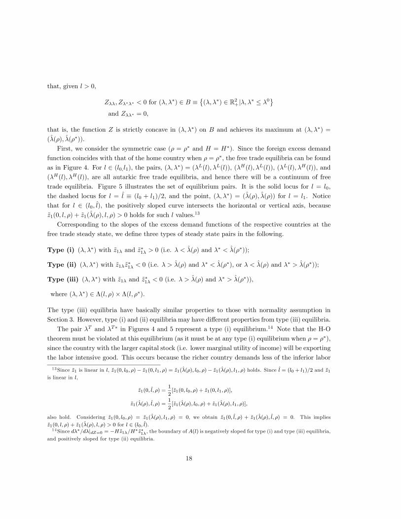
First, we consider the symmetric case (� = �� and H = H�). Since the foreign excess demand
function coincides with that of the home country when � = ��, the free trade equilibria can be found
as in Figure 4. For l 2 (l0;l1), the pairs, (�; ��) = (�L(l); �L(l)), (�H(l); �L(l)), (�L(l); �H(l)), and(�H(l); �H(l)), are all autarkic free trade equilibria, and hence there will be a continuum of free
trade equilibria. Figure 5 illustrates the set of equilibrium pairs. It is the solid locus for l = l0,
the dashed locus for l = l̂ � (l0 + l1)=2, and the point, (�; ��) = (�̂(�); �̂(�)) for l = l1. Notice
that for l 2 (l0; l̂), the positively sloped curve intersects the horizontal or vertical axis, because
~z1(0; l; �) + ~z1(�̂(�); l; �) > 0 holds for such l values.13
Corresponding to the slopes of the excess demand functions of the respective countries at the
free trade steady state, we de�ne three types of steady state pairs in the following.
Type (i) (�; ��) with ~z1� and ~z�1� > 0 (i.e. � < �̂(�) and �� < �̂(��));
Type (ii) (�; ��) with ~z1�~z�1� < 0 (i.e. � > �̂(�) and �� < �̂(��), or � < �̂(�) and �� > �̂(��));
Type (iii) (�; ��) with ~z1� and ~z�1� < 0 (i.e. � > �̂(�) and �� > �̂(��)),
where (�; ��) 2 �(l; �)� �(l; ��).
The type (iii) equilibria have basically similar properties to those with normality assumption in
Section 3. However, type (i) and (ii) equilibria may have di¤erent properties from type (iii) equilibria.
The pair �T and �T� in Figures 4 and 5 represent a type (i) equilibrium.14 Note that the H-O
theorem must be violated at this equilibrium (as it must be at any type (i) equilibrium when � = ��),
since the country with the larger capital stock (i.e. lower marginal utility of income) will be exporting
the labor intensive good. This occurs because the richer country demands less of the inferior labor
13Since ~z1 is linear in l, ~z1(0; l0; �)� ~z1(0; l1; �) = ~z1(�̂(�); l0; �)� ~z1(�̂(�); l1; �) holds. Since l̂ = (l0 + l1)=2 and ~z1is linear in l,
~z1(0; l̂; �) =1
2[~z1(0; l0; �) + ~z1(0; l1; �)];
~z1(�̂(�); l̂; �) =1
2[~z1(�̂(�); l0; �) + ~z1(�̂(�); l1; �)];
also hold. Considering ~z1(0; l0; �) = ~z1(�̂(�); l1; �) = 0, we obtain ~z1(0; l̂; �) + ~z1(�̂(�); l̂; �) = 0. This implies
~z1(0; l; �) + ~z1(�̂(�); l; �) > 0 for l 2 (l0; l̂).14Since d��=d�jdZ=0 = �H~z1�=H�~z�1�, the boundary of A(l) is negatively sloped for type (i) and type (iii) equilibria,
and positively sloped for type (ii) equilibria.
18

intensive good, and this e¤ect dominates its relatively lower supply of the labor intensive good at
these equilibria. The pair (�T 0; �T�) in Figures 4 and 5 is an example of a type (ii) equilibrium.
Note that the H-O theorem is also violated in this equilibrium, although it is not necessarily violated
at all type (ii) equilibria (e.g. the type (ii) equilibrium in which the home country is at �T ).15
We know from Proposition 4 that a steady state equilibrium will be a saddle point if (~z1� +
mH�
H ~z�1�) < 0. This condition is satis�ed for type (iii) equilibria, but must clearly fail for type (i)
equilibria. In contrast, type (ii) equilibria with �� < �̂(��) (�� > �̂(��)) will be saddle-point stable
if and only if the frontier of A(l) is steeper (more gradual) than the ray from the origin at that point:
d��
d�
����dZ=0
= � H~z1�H�~z�1�
(> ��=� = m if ~z�1� > 0;
< ��=� = m if ~z�1� < 0:(34)
Point S in Figure 5 is one example of type (ii) equilibrium where (34) holds.
For the equilibria where (~z1�+mH�
H ~z�1�) > 0 (J(0) < 0), Lemma 3 shows that the local dynamics
will be determined by the sign of J(� + ��). Evaluating this expression at � = �� using (28), we
obtain J(2�) = 2��3�J(0) > 0, which implies that a steady state is a source when it is not a saddlepoint and discount rates are identical.16
Based on the above, we obtain the following Proposition, which shows that the H-O theorem will
be violated at some steady states with the saddle-point stability, even if discount rates are identical.
Proposition 7 Let � = �� and H = H� hold. For l 2 (l0; l̂], there exist type (ii) equilibria wherethe H-O theorem is violated while the saddle-point stability holds.
Proof. Let m0(l) � �L(l)=�H(l), which is positive for l 2 (l0; l1). Since the positively slopedcurve intersects the horizontal axis for l 2 (l0; l̂], there is at least one intersection between the curveand the ray from the origin �� = m� with m < m0(l) where (34) holds (e.g. point S in Figure 5).
Since � 2 (�̂(�); �H(l)) and �� 2 (0; �L(l)) holds here, ~k < ~k� and ~z1 > 0 > ~z�1 are satis�ed, that is,the capital abundant foreign exports labor intensive good 1 at the equilibrium: the H-O theorem is
violated.
In the rest of this section, we shall consider the asymmetric case with � > ��. And we rede�ne
l0 and l1 as17
lim�;��!0
Z(�; ��; l0) = 0 and Z(�̂(�); �̂(��); l1) = 0 (35)
15 It can be easily shown that when � = �� the H-O theorem holds if and only if the steady state value of � or ��
is greater than �H(l).16This is consistent with �ndings of Kehoe et al [15], who have shown that dynamic indeterminacy cannot arise
in a one sector growth model with a �nite number of in�nitely lived agents and complete markets. If � = ��, the
equilibrium under factor price equalization will result in a Pareto optimal allocation in the H-O model even without
the existence of markets for borrowing and lending.17 If � = ��, these values correspond to the previous ones, which is associated with the existence of two autarkic
steady states in Proposition 6.
19

and modify Assumption 6 as follows:
Assumption 6�:
�� > �r0(~p)max����2 � ~p2
~p;���2 � 2~p� + ~p2
� � ~p
�:
Notice that18
�k(l; �)
l<�k(l; ��)
l; �̂(�) > �̂(��); and ~�max(l; �) < ~�max(l; ��): (36)
It is clear from the arguments below (18) that Z(~�max; ~��max; l) < 0 and from footnote 12 that if
� = ��, �k(l; �)=l < ~�max and ~�max(l; �) > �̂(�) hold for l 2 (l0; l1). So, as long as the di¤erencebetween � and �� is small, we have for l 2 (l0; l1),
�k(l; ��)=l < ~�max and ~�max(l; �) > �̂(�) (37)
and
Z(~�max; m̂~�max; l) < 0; (38)
where m̂ � �̂(��)=�̂(�) < 1, and hence m̂~�max < ~��max. (36) and (37) imply
~�min(l; �) = ~�min(l; ��) = 0 and �̂(��) < �̂(�) < ~�max(l; �) < ~�max(l; ��) for l 2 (l0; l1):
If the ray from the origin cuts twice the boundary of A(l) on �(l; �)��(l; ��), then one of themis type (i) or type (ii) equilibrium with J(0) < 0, while the other is type (iii) or type (ii) equilibrium
with J(0) > 0. The following Proposition shows the existence of such two intersections for some
range of values of m.
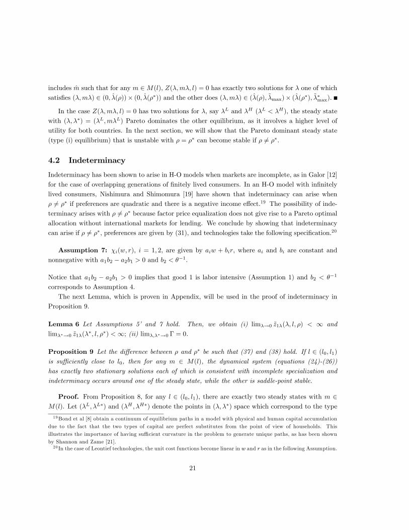
Proposition 8 Let the di¤erence between � and �� be such that (37) and (38) hold. For l 2(l0; l1), there exists an open interval M(l) such that for any m 2 M(l), Z(�;m�; l) = 0 has exactlytwo solutions for � one of which corresponds to type (i) equilibrium and the other does type (iii)
equilibrium.
Proof. Consider Z(�; ��; l) along the ray �� = m̂� which passes through (�̂(�); �̂(��)). Z is
increasing in � on [0; �̂(�)) and decreasing in � on (�̂(�);1). Note that for l 2 (l0;l1), Z(0; 0; l) < 0and Z(�̂(�); �̂(��); l) > 0 from (35) and Z(~�max; m̂~�max; l) < 0 from (38). Therefore, along the ray
�� = m̂�, Z changes its sign twice as � increases from 0 to ~�max, which implies that �� = m̂� cuts
twice the boundary ofA(l) and one intersection corresponds to type (i) equilibrium and the other does
type (iii) equilibrium (see Figure 5). So, for each l 2 (l0;l1), we can �nd an open interval M(l) that18 �k(l; �) = [E(~p; 0)� ~wl]=� is decreasing in �, �̂(�) is increasing in � from footnote 11, and ~�max(l; �) is decreasing
in � from Figure 3.
20
includes m̂ such that for any m 2M(l), Z(�;m�; l) = 0 has exactly two solutions for � one of whichsatis�es (�;m�) 2 (0; �̂(�))� (0; �̂(��)) and the other does (�;m�) 2 (�̂(�); ~�max)� (�̂(��); ~��max).
In the case Z(�;m�; l) = 0 has two solutions for �, say �L and �H (�L < �H), the steady state
with (�; ��) = (�L;m�L) Pareto dominates the other equilibrium, as it involves a higher level of
utility for both countries. In the next section, we will show that the Pareto dominant steady state
(type (i) equilibrium) that is unstable with � = �� can become stable if � 6= ��.
4.2 Indeterminacy
Indeterminacy has been shown to arise in H-O models when markets are incomplete, as in Galor [12]
for the case of overlapping generations of �nitely lived consumers. In an H-O model with in�nitely
lived consumers, Nishimura and Shimomura [19] have shown that indeterminacy can arise when
� 6= �� if preferences are quadratic and there is a negative income e¤ect.19 The possibility of inde-terminacy arises with � 6= �� because factor price equalization does not give rise to a Pareto optimalallocation without international markets for lending. We conclude by showing that indeterminacy
can arise if � 6= ��, preferences are given by (31), and technologies take the following speci�cation.20
Assumption 7: �i(w; r), i = 1; 2, are given by aiw + bir, where ai and bi are constant and
nonnegative with a1b2 � a2b1 > 0 and b2 < ��1.
Notice that a1b2 � a2b1 > 0 implies that good 1 is labor intensive (Assumption 1) and b2 < ��1
corresponds to Assumption 4.
The next Lemma, which is proven in Appendix, will be used in the proof of indeterminacy in
Proposition 9.
Lemma 6 Let Assumptions 5� and 7 hold. Then, we obtain (i) lim�!0 ~z1�(�; l; �) < 1 and
lim��!0 ~z1�(��; l; ��) <1; (ii) lim�;��!0 � = 0.
Proposition 9 Let the di¤erence between � and �� be such that (37) and (38) hold. If l 2 (l0; l1)is su¢ ciently close to l0, then for any m 2 M(l), the dynamical system (equations (24)-(26))
has exactly two stationary solutions each of which is consistent with incomplete specialization and
indeterminacy occurs around one of the steady state, while the other is saddle-point stable.
Proof. From Proposition 8, for any l 2 (l0; l1), there are exactly two steady states with m 2M(l). Let (�L; �L�) and (�H ; �H�) denote the points in (�; ��) space which correspond to the type
19Bond et al [8] obtain a continuum of equilibrium paths in a model with physical and human capital accumulation
due to the fact that the two types of capital are perfect substitutes from the point of view of households. This
illustrates the importance of having su¢ cient curvature in the problem to generate unique paths, as has been shown
by Shannon and Zame [21].20 In the case of Leontief technologies, the unit cost functions become linear in w and r as in the following Assumption.
21

(i) and type (iii) equilibrium, respectively. Then, the steady state with (�H ; �H�) is saddle-point
stable. On the other hand, J(0) is negative at the steady state with (�L; �L�). Let JL(� + ��) be
the value of J(� + ��) at the steady state with � = �L. The result will be established by showing
that JL(�+ ��) < 0. From equation (28), we obtain JL(�+ ��) to be
JL(�+ ��) = � (�+ ��)(�� ��)~z1r0(~p)
+ ����(�+ ��)� �
r0(~p)
��2~z1� + �
�2mH�
H~z�1�
�;
where r0(~p) is given by �a2=(a1b1�a2b1) under Assumption 7. Note that for anym both �L and �L�
(= m�L) go to 0 as l goes to l0. From Lemma 6, the last term in parentheses is bounded, so the last
term will approach 0 as �; �� ! 0. Also, we see that the second term will approach 0 as �; �� ! 0. For
the �rst term, we have liml!l0 ~z1(�L; l; �) < 0, because Z(0; 0; l0) = H~z1(0; l0; �)+H�~z1(0; l0; �
�) = 0
and @~z1=@� = r0(~p)~k=� < 0 together imply that ~z1(0; l0; �) < 0. Therefore, JL(� + ��) is negative
when l is su¢ ciently close to l0. Thus, from Lemma 3, the characteristic equation has two roots
with negative real parts at the steady state with � = �L, which implies that indeterminacy occurs
around the steady state.
The possibility of dynamic indeterminacy in a two country trade model when there are no markets
for international lending and borrowing has been previously shown Shimomura [23] and Doi et al.
[11] for the case of an endowment model of international trade in which one of the goods is durable
and there is a negative income e¤ect. Nishimura and Shimomura [19] discussed the possibility of
dynamic indeterminacy in a two country H-O model, where they supposed � 6= �� and a speci�c
utility function and Leontief technologies with b1 = 0 and a2 = b2 = 1, and derived some conditions
under which indeterminacy occurs around the steady state. However, their focus is mainly on the
occurrence of indeterminacy and they did not considered the multiplicity of the steady states in
our model. Indeed, one can verify that in their model, there is no possibility of the multiplicity
because the negatively sloped region in their excess demand function is inconsistent with incomplete
specialization under their assumed preferences and technologies.
Bond and Driskill [9] have shown that inferiority in consumption is not necessary to generate
multiple steady states and indeterminacy in the model with durable consumption goods: indetermi-
nacy can arise when both goods are normal as long as the exporting country has the higher marginal
propensity to consume a good. In contrast, our results here show that inferiority in consumption
is a necessary condition for the existence of multiple steady states and indeterminacy in the H-O
model when factor price equalization holds. The di¤erence between the two cases is due to the
fact that with the factor price equalization property, the marginal utility of consumption in the two
countries must be moving in the same direction along the optimal path. The H-O model of trade
we examine here also requires that trade balance at each point in time. However, if there is factor
price equalization along the optimal path, international lending and borrowing is redundant if the
discount factors of the two countries are the same. As a result, a di¤erence in discount factors
between countries and inferiority in consumption are both necessary conditions for indeterminacy
22

to occur.
5 Concluding Remarks
Our analysis have shown that the many of the results of the dynamic H-O model will extend to
the case of non-homothetic preferences as long as both goods are normal and discount factors are
the same between countries. In this case the steady state trade pattern will satisfy the static H-O
theorem, a dynamic H-O theorem will hold, and the steady states will be saddle points. The main
di¤erence introduced by non-homotheticity when goods are normal and discount factors are equal
is that the world capital stock will depend on the distribution of income across countries. Allowing
discount factors to di¤er between countries (while keeping steady state rentals constant) introduces
the possibility that the static and dynamic H-O theorems may fail to hold.
We have also provided an example to show that the results may di¤er dramatically if the labor
intensive good is inferior. These di¤erences include the possibility that there are multiple steady
state equilibria, that the static H-O theorem is violated in the steady state, and that some steady
state equilibria are Pareto dominated. If discount factors are the same across countries, steady state
equilibria will be either saddle points or unstable equilibria. However, if discount factors di¤er across
countries there is the possibility of local indeterminacy.
6 Appendix
6.1 Proof of Lemma 1
Totally di¤erentiating equations (8) with respect to c1, c2, p and �, we derive"u11 u12
u21 u22
#"dc1
dc2
#=
"p
1
#d�+
"�
0
#dp:
Since the determinant of the coe¢ cient matrix, D = u11u22 � u212, is positive at any point whereui(c1; c2) > 0 (Assumption 2) and therefore invertible, we obtain
c1�(p; �) �@c1@�
=1
D(u22p� u12); (39)
c2�(p; �) �@c2@�
=1
D(u11 � u12p); (40)
c1p(p; �) �@c1@p
=1
D�u22 < 0; (41)
c2p(p; �) �@c2@p
= � 1D�u12: (42)
The results of Lemma 1 follow immediately from these comparative statics results.jj
23

6.2 Derivation of the Characteristic Equation (28)
Expanding (27) yields
det [xI � J ] = x3 ���+ �� � �r0 @p
@���z1 + �c1� + (z
�1 +m�c
�1�)
H�
H
�@p
@k
�x2
+
���� � (�+ ��)�r0 @p
@����� (z1 + �c1�) + � (z
�1 +m�c
�1�)
H�
H+
�E� +m
H�
HE��
��r0�@p
@k
�x
+ �r0����
@p
@�+
���E� + �m
H�
HE��
�@p
@k
�: (43)
Since Hz1 +H�z�1 = 0 at the world trade equilibrium and r0 @p@� + (c1� +mH�
H c�1�)
@p@k = 0 from (23),
the coe¢ cient of x2 becomes � (�+ ��). Using the latter equation to substitute into the coe¢ cienton x and the constant term yields
��� ��(�� � �)z1 � � (�c1� � r0E�)� �m
H�
H(��c�1� � r0E��)
�@p
@k
and � ���� (�c1� � r0E�) + �m
H�
H(��c�1� � r0E��)
�@p
@k;
respectively. Multiplying the result by � ���r0 @p@k
��1and using (19) yields (28) in the text.
6.3 Proof of Lemma 4
Let � � f(c1; c2) 2 R2+j0 < c�1 c2 < � and 0 < c1c�2 < �g, which is the set of (c1;c2) for which
ui(c1; c2) > 0 for i = 1; 2. It is straightforward to show that (31) is strictly concave over the subset
� when Assumption 5� is satis�ed. The proof that the solutions to (8) are unique proceeds in
two steps, which will only be sketched here. First, establish that any element of � has a unique
representation as (c1; c2) =�h
(s�)�
v� ��1
i 1���1
;h(v�)�
s� ��1
i 1���1
�for 0 < s; � < 1. Second, substitute this
representation into (8) and show that the resulting equations have unique solutions s(p; �); �(p; �) 2(0; 1) for any positive p and �. Furthermore, these solutions have the properties that the respective
function are decreasing in � with lim�!0 s(p; �) = 1, lim�!1 s(p; �) = 0, lim�!0 v(p; �) = 1, and
lim�!1 v(p; �) = 0. Based on these two results, we can conclude that for any positive p and �, the
system of equations (8) has an unique, interior, and positive solution, (c1(p; �); c2(p; �)), where
c1(p; �) =
�[�s(p; �)]�
� ��1v(p; �)
� 1���1
; (44)
c2(p; �) =
�[�v(p; �)]�
� ��1s(p; �)
� 1���1
: (45)
(i) From equations (44) and (45), it is clear that lim�!0 c1(p; �) = �c1 and lim�!0 c2(p; �) = �c2,
since lim�!0 s(p; �) = 1 and lim�!0 v(p; �) = 1. On the other hand, from the �rst-order conditions
(equations (8)), we see that lim�!1 ci(p; �) = 0; i = 1; 2.
24
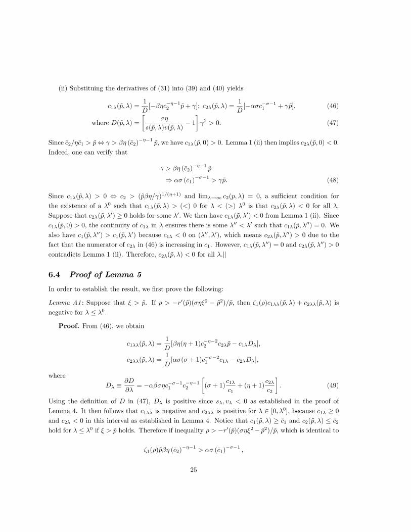
(ii) Substituing the derivatives of (31) into (39) and (40) yields
c1�(~p; �) =1
D[���c���12 ~p+ ]; c2�(~p; �) =
1
D[���c���11 + ~p]; (46)
where D(~p; �) =�
��
s(~p; �)v(~p; �)� 1� 2 > 0: (47)
Since �c2=��c1 > ~p, > �� (�c2)���1
~p, we have c1�(~p; 0) > 0. Lemma 1 (ii) then implies c2�(~p; 0) < 0.
Indeed, one can verify that
> �� (�c2)���1
~p
) �� (�c1)���1
> ~p: (48)
Since c1�(~p; �) > 0 , c2 > (~p��= )1=(�+1) and lim�!1 c2(p; �) = 0, a su¢ cient condition for
the existence of a �0 such that c1�(~p; �) > (<) 0 for � < (>) �0 is that c2�(~p; �) < 0 for all �.
Suppose that c2�(~p; �0) � 0 holds for some �0. We then have c1�(~p; �0) < 0 from Lemma 1 (ii). Since
c1�(~p; 0) > 0, the continuity of c1� in � ensures there is some �00 < �0 such that c1�(~p; �00) = 0. We
also have c1(~p; �00) > c1(~p; �0) because c1� < 0 on (�00; �0), which means c2�(~p; �00) > 0 due to the
fact that the numerator of c2� in (46) is increasing in c1. However, c1�(~p; �00) = 0 and c2�(~p; �00) > 0
contradicts Lemma 1 (ii). Therefore, c2�(~p; �) < 0 for all �.jj
6.4 Proof of Lemma 5
In order to establish the result, we �rst prove the following:
Lemma A1 : Suppose that � > ~p. If � > �r0(~p)(���2 � ~p2)=~p, then �1(�)c1��(~p; �) + c2��(~p; �) is
negative for � � �0.
Proof. From (46), we obtain
c1��(~p; �) =1
D[��(� + 1)c���22 c2�~p� c1�D�];
c2��(~p; �) =1
D[��(� + 1)c���21 c1� � c2�D�];
where
D� �@D
@�= �����c���11 c���12
�(� + 1)
c1�c1+ (� + 1)
c2�c2
�: (49)
Using the de�nition of D in (47), D� is positive since s�; v� < 0 as established in the proof of
Lemma 4. It then follows that c1�� is negative and c2�� is positive for � 2 [0; �0], because c1� � 0and c2� < 0 in this interval as established in Lemma 4. Notice that c1(~p; �) � �c1 and c2(~p; �) � �c2hold for � � �0 if � > ~p holds. Therefore if inequality � > �r0(~p)(���2� ~p2)=~p, which is identical to
�1(�)~p�� (�c2)���1
> �� (�c1)���1
;
25

holds, then
�1(�)~p��c���12 � �1(�)~p�� (�c2)���1
> �� (�c1)���1
� ��c���11 (50)
for � � �0. Based on the above, we obtain
�1(�)c1��(~p; �) + c2��(p̂; �)
=1
D
h�1(�)~p��(� + 1)c
���22 c2� � �1(�)c1�D� + ��(� + 1)c���21 c1� � c2�D�
i<1
D
���c���11
�(� + 1)
c1�c1+ (� + 1)
c2�c2
�� [�1(�)c1� + c2�]D�
�= �D�
D
"1
��c���12
+ �1(�)c1� + c2�
#
= �D�D
"�1(�)c1� +
D + (���c���11 + ~p)��c���12
D��c���12
#
= �D�D
"�1(�)c1� +
� 2 + ~p��c���12
D��c���12
#
= �D�D
"�1(�)c1� +
� c1���c���12
#
= � D�c1�
D��c���12
h�1(�)��c
���12 �
i� 0
for � � �0. Here the second inequality comes from (50), the third equality is due to (49), and the
last inequality comes from (48) and (50).
From Lemma A1, we see that the excess demand function (32) is strictly concave in � for
� 2 [0; �0].Next, it is apparent from (46) that
�1(�)[ � �� (�c2)���1 ~p] > �� (�c1)���1 � ~p ) �1(�)c1�(~p; 0) + c2�(~p; 0) > 0:
One can easily verify that the former inequality is identical to inequality � > �r0(~p)(���2 � 2~p� +~p2)=(� � ~p) under � > ~p.
Therefore, ~z1�� < 0 for � 2 [0; �0] and ~z1�(0; l; �) > 0 if Assumptions 5�and 6 hold. Since bothc1� and c2� are negative for � > �0, it is apparent from the continuity of ci�; i = 1; 2, in � that
there is some �̂(�) < �0 such that
26

~z1�(�; l; �) = �r0(~p) [�1(�)c1�(~p; �) + c2�(~p; �)]
�
(> 0; if � < �̂(�);
< 0; if � > �̂(�);(51)
where �̂(�) is implicitly de�ned as the solution to ~z1�(�; l; �) = 0.jj
6.5 Proof of Lemma 6
From (13), (19), and (39)-(41), we obtain
~z1� = c1� �r0E��
=1
u11u22 � (u12)2
�u22~p� u12 � r0
u22~p2 � 2u12~p+ u11
�
�;
z1p = c1p �@y1@p
=�u22
u11u22 � (u12)2:
Notice that @y1=@p = 0 under Assumption 7. Since lim�!0 ci(p; �) = �ci 2 (0;1), i = 1; 2, we see
lim�!0
~z1�(�; l; �) <1 and lim�!0
z1p(~p; k; l; �) = 0:
Finally, from (23), we have
lim�;��!0
� = lim�;��!0
��r0 @p
@k
��1= lim
�;��!0
��Hz1p +H
�z�1pH(r0)2
�= 0:jj
27

References
[1] Atkeson, A., Kehoe, P.: Paths of development for early- and late-boomers in a dynastic
Heckscher-Ohlin model, Research Sta¤ Report 256, Federal Reserve Bank of Minneapolis, 2000
[2] Becker, R.: On the long-run steady state in a simple dynamic model of equilibrium with het-
erogeneous households, Quarterly Journal of Economics 95, 375�382, (1980)
[3] Benhabib, J., Farmer, R. E. A.: Indeterminacy and sector speci�c externalities, Journal of
Monetary Economics 37, 397�419, (1996).
[4] Benhabib, J., Farmer, R. E. A.: Indeterminacy and growth,�Journal of Economic Theory 63,
19�41 (1994)
[5] Benhabib, J., Meng, Q., Nishimura, K.: Indeterminacy under constant returns to scale in
multi-sector economies, Econometrica 68, 1541�1548, (2000)
[6] Benhabib, J., Nishimura, K.: Indeterminacy and sunspots with constant returns, Journal of
Economic Theory 81, 58�96, (1998)
[7] Boldrin, M., Rustichini, A.: Indeterminacy of equilibria in models with in�nitely-lived agents
and external e¤ects, Econometrica 62, 323�342, (1994)
[8] Bond, E., Trask, K., Wang, P.: Factor accumulation and trade: dynamic comparative advantage
with endogenous physical and human capital, International Economic Review 44, 1041�1060,
(2003)
[9] Bond, E, Driskill, R:�Multiplicity and Stability of Equilibrium in Trade Models with Durable
Goods,in T. Kamihigashi and L. Zhao (eds), International Trade and Economic Dynamics:
Essays in Honor of Koji Shimomura, Springer-Verlag, (2008).
[10] Chen, Z.: Long-run equilibria in a dynamic Heckscher-Ohlin model, Canadian Journal of Eco-
nomics 25, 923�943, (1992)
[11] Doi, J., Iwasa, K., Shimomura, K.: Indeterminacy in the free-trade world, Journal of Di¤erence
Equations and Applications 13, 135�149, (2007)
[12] Galor, O: A Two Sector Overlapping Generations Model: A Global Characterization of the
Dynamical System, Econometrica, 60, 351-386, (1992).
[13] Galor, O. and S. Lin, �Dynamic Foundations for the Factor Endowment Model of International
Trade,� in B. S. Jensen and K. Wong, eds., Dynamics, Economic Growth, and International
Trade (Ann Arbor, MI: University of Michigan Press, 1997).
28

[14] Iwasa, K., Shimomura, K.: A family of utility functions which generate Gi¤en paradox, The
Journal of Economics of Kwansei Gakuin University 60(3), 29�45, (2007)
[15] Kehoe, P, Levine, D, Romer, P: Determinacy of Equilibria in Models with Finitely Many
Consumers, Journal of Economic Theory, 50 (1), 1-21, 1990.
[16] Mino, K. : Indeterminacy and endogenous growth with social constant returns, Journal of
Economic Theory 97, 203�222, (2001)
[17] Nishimura, K., Shimomura, K.: Indeterminacy in a dynamic small open economy, Journal of
Economic Dynamics and Control 27, 271�281, (2002)
[18] Nishimura, K., Shimomura, K.: Trade and indeterminacy in a dynamic general equilibrium
model, Journal of Economic Theory 105, 244�259, (2002)
[19] Nishimura, K., Shimomura, K.: Indeterminacy in a dynamic two-country model, Economic
Theory 29, 307�324, (2006)
[20] Routh, E. J.: The advanced part of a treatise on the dynamics of a system of rigid bodies, 6th
edn. London: Macmillan (1905), Reprinted in A. T. Fuller ed., Stability of motion, London:
Taylor & Francis (1975)
[21] Shannon, C, and Zame, W: Quadratic Concavity and Determinacy of Equilibrium, Economet-
rica, 70 (2), 631-662, (2002).
[22] Shimomura, K.: A two-sector dynamic general equilibrium model of distribution, in: G. Fe-
ichtinger ed., Dynamic Economic Models and Optimal Control, North-Holland, 105�123, (1992)
[23] Shimomura, K.: Indeterminacy in a dynamic general equilibrium model of international trade,
in: M. Boldrin, B-L Chen, and P. Wang eds., Human Capital, Trade and Public Policy in
Rapidly Growing Economies: From Theory to Empirics, Cheltenham: Edward Elgars, 153�167,
(2004)
[24] Stiglitz, J. E: Factor Price Equalization in a Dynamic Economy, Journal of Political Economy
78, 456-488, (1970).
[25] Ventura, J: Growth and Interdependence, Quarterly Journal of Economics, 112, 57-84, (1997).
29

Figure 1
1( , , )z l
O
A max( , )l
min ( , )l
0 1

Figure 2
( )K H k 45 The line
( )K HkO
* * KK H
H
(i)(ii)

max
Figure 3
( , , ) ( , )k l E p wl
l l
k l
min ( , )l max ( , )l
min
O
l

Figure 4
( )L l ( )H l l
O
1( , , )z l
ˆ( )
0H
( )l ( )l
0l l
1l lT
T T

Figure 5
0H
45 The line
l
0l l
ˆl l(ii)
ˆ( )
ˆ( )H l
ˆ( )L l
OS
m
l
T
T T
(iii)
(ii)
(i) 1l l
ˆl l