1

Keeping up with the Joneses:

Inequality and Indebtedness, in the Era of the Housing Price Bubble, 1999-2007*

Neil Fligstein, Pat Hastings, and Adam Goldstein

Department of Sociology

University of California

Berkeley, Ca. 94610

August 2015

* This project was partially supported by a grant from the Institute for New Economic Thinking.

It was also supported by funds from the Institute for Research on Labor and Employment at the

University of California. This paper was presented at the Annual Meetings of the American

Sociological Association, Chicago, IL. Aug. 22-25, 2015.

2

Abstract

Sociologists have conceptualized lifestyles as structured hierarchically where those in a lower

group seek to emulate those higher up. Growing income inequality in the U.S. has meant that as

those at the top are able bid up the price of valued goods like housing and access to good

schools, those in lower groups have struggled to maintain their positions. We examine this

process in the context of the U.S. housing market from 1999-2007 using the Panel Study of

Income Dynamics. Houses are the ultimate status symbol. Their size, quality, and location signal

to others that one has (or has not) arrived. As house prices rose, we show through an analysis of

residential moves that upper income households (80-100% in the income distribution) upgraded

their houses by relocating to more expensive zip codes and larger houses in their quest to

maintain their status. Those in the bottom 50% of the income distribution found it difficult to

participate in the housing market at all and frequently moving to lower priced rentals. When they

did buy, rising prices pushed them to increase their share of expenditure on housing and their

mortgage debt-to-income ratio even when they did not upgrade house size or neighborhood.

Those in the middle (50-80%) were stretched thin but kept up. Households who had children

were particularly willing to increase their housing expenditure share and indebtedness. This

evidence implies that growing inequality meant a struggle to maintain lifestyles during the

housing bubble in particular for the bottom 50% of the income distribution.

3

Introduction

Sociologists have explored the relationship between inequality and lifestyle competition

by focusing on consumption (Bourdieu 1984; Sobel 1980; Schor 1998). The basic argument has

been that the consumption of goods reflects social status. Since 1980 in the U.S., the struggle

over lifestyle has been compounded by increasing income inequality. As income inequality has

grown at the top, this has placed pressures on those below to work to keep up despite stagnant

incomes for most households. Households have had to struggle to stay where they are in the

status hierarchy and many have fallen behind (Schor 1998; Leicht and Fitzgerald 2006; Frank

2007b).

One of the most acute manifestations of this intensified lifestyle pressure can be seen in

the rising costs of housing. House prices increased by almost 100% during 1995-2007 (Shiller,

2008). The U.S. Census Bureau estimated that by 2004, over 40% of households could not afford

a home priced in the bottom quartile of the local market where they resided (Savage 2009).

Schwartz and Wilson (2008) found that in 2006, 47% of renters and 36% of mortgaged

homeowners had monthly housing costs that exceeded the conventional 30% of income cutoff

for housing affordability. Most households tried to preserve their style of life by going deeper

into debt (Ragan, 2010; Langley, 2008;, 2012; Porter, 2012, Manning, 2001; Cynamon and

Fazzari 2009). One of the key areas in which debt grew the most was for housing (Goldstein,

2014).

In this paper we elaborate a lifestyle competition theory of consumption and apply it in

order to explain the patterns by which Americans have responded to the twin pressures of rising

inequality and the rising housing costs. As the richest people bid up the prices for housing in the

most desirable neighborhoods, this forced the households who had income right below them to

4

have to buy less expensive houses, but at a higher price (Frank 2007a). This competition

cascades through the housing market forcing people lower down to take on more debt or forego

buying a house all together. The house price bubble of 1995-2007 offers us an opportunity to

observe this process in action. We know that in order to keep up, households had to learn to be

more accepting of going into debt and taking financial risks (Fligstein and Goldstein, 2015;

Akerlof and Shiller, 2010).

In this paper, we look for empirical evidence of such status competition during this

period. We use the Panel Study of Income Dynamics (hereafter, PSID) to show how households

responded to lifestyle pressures in the housing market. The PSID allows us to determine whether

or not households moved in a two year time period. It also provides information on the housing

status of a household at the first time point (i.e. owning or renting) and where the household

ended up. The PSID also provides us with information on why people moved. We are able to

assess for those who moved whether they thought they were upgrading or downgrading their

housing quality. We examine how those who upgraded (and downgraded) their housing explains

changes in the size of the houses people inhabit, the kinds of neighborhoods different people

move to, the amount of debt they take on, and the amount of money they expend each month on

housing.

Recent work by sociologists and economists has explored the relationship between

inequality and housing consumption using cross-sectional data from the Consumer Expenditure

Survey (hereafter, CEX) (Charles and Lundy 2012; Bertrand and Morse 2013). We build on

these studies in several ways. The CEX contains great detail on how much households spend on

a given consumption category, but it does not tell us anything about the nature of the goods they

are purchasing. The PSID allows us to analyze the amount people are spending and borrowing

5

for housing as well as the quality of the housing they are consuming (size of the house and

neighborhood desirability). The longitudinal structure of PSID allows us to observe individuals

across time and space as they move across housing markets. We can draw inferences from the

behavior of the same households over time rather than from cross sectional differences. Finally,

we move beyond looking at the average effects of these changes by assessing how house price

changes across place affect different parts of the income distributions in different ways.

Not surprisingly, our results show that income is highly related to home ownership. Only

10% of households in the bottom 10% of the income distribution owned homes while 95% in the

top 10% of the income distribution owned homes in 2007. During the period 1999-2007, only

27% of the moves made by households in the bottom 50% of the income distribution were

people moving to owning homes while 78% of the moves made by those in the 81-100% of the

income distribution were people moving to own homes. Growing income inequality and rising

housing prices meant that the bottom 50% of the income distribution were not able to buy houses

as prices went up and when they moved they were more likely to downsize their housing. The

top 50% were more likely to be home buyers and mostly they were trying to upgrade their

housing.

We do find evidence that households at all levels of the income distribution who did

move to upgrade their housing did so in order to get more space and be in better neighborhoods.

But they also faced going deeper into debt and making larger house payments. Everyone across

the income distribution who did try and “keep up with the Jones” by upgrading their housing in

the face of rising inequality and house prices were prepared to pay the price to do so. From our

perspective, this is evidence that status competition was present across the income distribution.

6

Our paper has the following structure. We elaborate how status competition works, and

how it bears on consumption and debt. Then, we apply this to the case of housing consumption

in the U.S. during the 2000s. We discuss the centrality of housing in Americans’ conception of

what constitutes a middle class lifestyle and how housing plays a key role in the competition for

social status. Next, we consider how rising income inequality has helped push up the prices of

houses during the housing bubble of 1995-2007. We propose some hypotheses about what this

implies for housing choices made at varying levels of the income distribution. Then we provide

data that supports our analysis. Finally, we conclude by considering how while the striving for a

better lifestyle continues, keeping up in the face of growing inequality is hardest for those in the

bottom 50% of the income distribution. .

Theoretical Considerations

It is useful to elaborate the concept of lifestyle competition. Weber defined social status

as a form of community where groups are formed around a specific, positive or negative form of

social honor (1946: 186). Status honor is normally expressed by members of a group through the

symbolic expression of a style of life. Elias (1994) took up Weber’s idea of social status and

offered a dynamic view of how status evolves through competitive interactions between groups.

Elias argued that a status order was constantly in flux as a result of individual and collective

strategies to emulate those above you in the status hierarchy.

Elias elucidates this perspective using the case of early modern European society (1994).

The social status of the nobility was a consequence of their claim on social honor due to their

privileged birth. In the 16th

and 17th

century, they became “civilized” by learning manners, new

7

styles of dress and consumption, and how to make polite and erudite conversation. As capitalism

took hold, new social groups began to emerge. These groups did not have noble birth, but some

of them, notably the richest merchants, had money. They worked to enter high society by

adopting the mannerisms of the nobility. Elias argues that this new rich merchant class had its

imitators in social strata just below them. Those with fewer resources worked to create what we

would now call middle class lifestyles. Below them who were less educated and had fewer

resources created working class culture but still aspired to have more.

Bourdieu’s Distinction (1984) built on Elias’ analysis by opening up new ground in the

empirical study of lifestyle. Lifestyle is conceived of as a set of dispositions that actors have but

they are manifested in the kinds of choices people make about how to consume. Bourdieu’s

theory emphasized that people learn about whom they are and what they should expect in life

from their class background. He argues that adults construct their lifestyles around two features

of their resources: cultural capital and economic capital. They construct their consumption on

their basis of their perception of who they are and who they are trying to emulate (or oppose). He

uses survey data to provide evidence for these divisions.

Schor pursues the theme of consumption and lifestyle in The Overspent American (1998).

She follows Elias’ and Bourdieu in positing that people strive to compete over status goods.

These goods help define peoples’ identities and signal to others, their social status. She uses

survey data to show how the process of keeping up with others is an arms race where upping the

spending ante, forces other to follow. She views the formation of consumer society as at least

partially the result of corporations taking advantage of people’s tendencies to consume more and

more in order to display their social status. Schor’s version of lifestyle and consumption focuses

8

on how individuals get caught up in status contests and will go into debt to continue to try and

keep up.

Frank (1989; 2007a; 2007b), an economist, has further elaborated a sociological way to

understand the relationship between inequality, positional competition and consumption. He

agrees with sociologists that status and ranking is important for consumption decisions. He

argues that consumption is done in relation to what other people have. When people are given

choices between owning a house that is 4,000 square feet but their neighborhoods have houses

averaging 6,000 square feet versus owning a house that is 3,000 square feet but their neighbors

average 2,000 square feet, they choose the latter (Frank 2007b). Frank makes the case that the

cost of positional goods (a term coined by Hirsch (1979)) can be driven up over time in the face

of constant or declining supply, particularly in a context of rising income inequality (2007). This

line of work emphasizes how the increasing concentration of income at the top has set off a

cascading arms race among everyone else that increases the price they must pay in order to

maintain a constant position vis a vis others.

From this literature we can identify two conceptually distinct mechanisms by which

lifestyle competition processes will affect consumption, expenditure, and debt. The first is that

lifestyle competition changes consumption by shifting what we seek to consume. As those who

we seek to emulate or keep up with spend more, we are pushed to spend more as well. Simple

versions might involve emulative consumption of the rich, such as the phenomenon of large

“McMansions” marketed to middle-class homebuyers during the 1990s and 2000s (Schor 1998;

Dwyer 2009). Increasingly lavish consumption at the top may also indirectly fuel higher

absolute consumption throughout the distribution by inflating the cultural standards of what is

considered relatively normal or even modest for those further below (Levine, et. al. 2010).

9

The second mechanism is how prices for valued goods can be bid up as income

inequality increases. A greater concentration of income near the top of the distribution will tend

to inflate prices for the most desirable goods. Rising inequality can ratchet up individuals’

relative consumption preferences by intensifying demand for scarce positional goods. For

example, growing inequality may prompt more parents to seek access to the very best schools by

triggering anxiety about class reproduction in an increasing winner-take-all society (Rivera and

Lamont 2012; Frank 2007b). Price cascades are particularly applicable in the case of residential

real estate, where increasing prices at the top of the local market will tend to reverberate

throughout the market (Matlock and Vigdor 2010). This means that where there is greater

income inequality, median housing prices are higher (Levine et al 2010). The implication is that

in order to maintain a given lifestyle, people will have no choice but to pay more.1

Middle Class Aspirations, Housing, Debt, and Inequality

Home ownership has been the aspirational goal of the middle class in the U.S. since the

1920s (Megbolugbe and Linneman, 1993). It has signified “arriving” at a certain status (Dupuis

and Thorns, 2002). Polls have consistently revealed that a middle class lifestyle in the U.S.

requires having a house, car, a good job, some wealth, and enough money to pay for one’s

children’s college (Schor, 1998; 10-16). Roper Polls have been tracking attitudes towards what

constitutes a “good life” in the U.S. since 1975. The leading category for the past 40 years has

been home ownership: 85% of Americans in 1975 saw houses as necessary to have a “good life”,

87% in 1991, and 89% in 2001. The second highest category is a happy marriage: 84% saw a

1 It difficult to measure directly the effect of these two mechanisms. Here, we examine a historical period where

we know housing prices were on the rise in order to see how households at different income levels responded. That rise was a result of both of these mechanisms.

10

good life as a happy marriage in 1975, 77% in 1991, and 75% in 2001. Note that owning a house

rates slightly above having a good marriage for having the good life. Pew Research Center, on

the eve of the recent financial crisis, issued a report on the state of middle class America. In their

survey they report that middle class Americans “regard their home as their most important asset

and the anchor of their lifestyle” (2008:33).

From the perspective of competition over lifestyles, houses are the ultimate positional

good. They are expensive, their size can vary, and the quality of building materials and locational

amenities mean that they can become an important focus of status competition. Moreover,

housing often gives access to good schools for children, another kind of positional good.

Evidence shows that parents are willing to pay 2.5% more for a house for a 5% increase in test

scores (Black, 1999). This is particularly true for the best schools, those in the highest test score

brackets (Clapp, et. al. 2008). The fact that housing is at the core of middle class aspirations and

the fact that it is likely to be a place where groups with different amounts of income compete

over the qualities of housing (and schools), makes it an ideal site to study lifestyle competition.

Increases in income inequality have been ongoing since the early 1980s (Atkinson, et. al.

2011). The increase in income inequality has been accompanied by an increase in labor market

risks of all sorts (for reviews, see Fligstein and Shin 2004; Kalleberg 2009; Western, et. al, 2012).

In the face of rising inequality, it follows that the lifestyles of households at any level of that

distribution proved more difficult to maintain particularly relative to those who were situated just

above you. As the share of income at the top of the distribution increased, it put pressure on those

below to try to keep up (Frank 2007b; Charles and Lundy 2012). These pressures extended down

all the way to the bottom of the distribution where incomes were declining both in constant and

relative terms (Atkinson, et. al. 2011).

11

In the past 25 years, the easiest way to close the gap between what you were earning and

what you needed to preserve your position was to borrow money. To accomplish this, there had to

be a huge expansion of credit (Rajan 2010; Hyman 2011; Erturk, et. al. 2007). Numerous scholars

have argued that, in the aggregate, credit expansion allowed Americans to counter their stagnant

incomes and economic insecurity, thereby maintaining their lifestyles and positions in the status

hierarchy (Hacker, 2006; Leicht and Fitzgerald, 2006; Rajan 2010; McCloud and Dwyer, 2011).

Credit thereby supplied the fuel by which households could engage in aggressive lifestyle

competition as prices rose and incomes remained stagnant.

But this expansion of credit did not really level the playing field. If everyone increases

their indebtedness, then the status position between groups remains unchanged. Frank (2007b)

describes this as a positional arms race that inevitable will be won by those with more money.

House prices increased in the U.S. between 1996 and their peak in 2005 from an average of

$160,000 to $230,000 for existing homes and $140,000 to $230,000 for new homes (Fligstein

and Rucks Ahidiana, forthcoming).2 As the richest people who lived in a particular area come to

bid up the prices for the best houses located near the best schools, this pushed people who are

competing with them to bid up the prices of the next tier of housing. Worse still, it means that the

farther you go down the income distribution, the more likely that households will have to forego

buying houses. Rising rents, which track house prices, may also push them into worse

neighborhoods.

Aggregate trends and results from several related studies do offer suggestive evidence for

the idea that lifestyle competition for housing has occurred, and that it was driving households to

consume more and to take on more debt. In terms of housing size, the U.S. Census Bureau

2 Housing prices dropped dramatically from 2007-2009 but they resumed their upward growth from 2009-2013 and

in 2015 are near the levels reached in 2005.

12

(2011) shows that house size averaged 1,645 feet in 1975, 2,080 in 1990, 2,223 in 2000, and

2,392 in 2010.3 This process is consistent with a positional arms race where those who are richer

want bigger houses and those below them respond by demanding the same. We know that

spending on housing as a share of income and as a share of total expenditure increased for both

owners and renters during this period (Goldstein, 2014). Results from two recent household-level

studies using the Consumer Expenditure Survey find that median levels of consumption tend to

be higher in cities with higher inequality, controlling for the attributes of households in those

cities (Charles and Lundy 2012; Bertrand and Morse 2013). This is consistent with the idea that

consumption “trickles down”, either by ratcheting up standards or by bidding up prices.

We know that the precipitous growth indebtedness during this period was driven almost

exclusively by mortgage debt growth (Dynan and Kohn 2007; Goldstein, 2014). Debt-to-income

grew across the income distribution, but it grew the most among the upper middle-class

households, who are presumably most susceptible to competitive status pressures from those at

the top (Goldstein 2012). Fligstein and Goldstein (2015) show that these changes have been

accompanied by a shift in cultural attitudes towards whereby taking risk and borrowing money to

maintain one’s lifestyle have become more normative. This is particularly true for the top 20% of

the income distribution where the direct effects of increasing income inequality are felt most

directly. Instead of settling for less, households became comfortable with buying as much house

as they could and accepting the higher levels of expenditure, debt, and risk that this entailed.

Research Design and Hypotheses

3 There is a huge literature in marketing and consumption that shows that over time, there has been a ratcheting up

of expectations for a wide variety of goods. See Schor (1998) and Zukin and Maguire (2008) for reviews.

13

The rapid house price increases of 1995-2007 offer us a site to observe how rapid price

increases in the most important positional lifestyle good impacted households at different parts

of the income distribution. Our basic argument is that people higher up in the income distribution

will be more likely to upgrade their housing than people lower down in the face of rising house

prices and thus, be able to “keep up with the Joneses”. Those lower down will face pressure

either to forego the opportunity to buy in the first place, have to move to a cheaper rental, or be

forced to sell their homes. They will be more likely to experience downward mobility in social

status.

Measuring the effect of income inequality and rising house prices on the ability of

households to upgrade or downgrade their housing in order to keep their position in the status

queue, needs unpacking. Our argument can be taken to imply implies that households are always

acting to worry about their status and that such a concern always drives their behavior. But in

reality, moving reflects not just status competition but a whole host of unrelated factors. People

who already own homes may have the view that they already have arrived and will thus be

disinterested in moving. People buy and sell houses not just for status, but also for changes in

their life circumstances like new jobs or retiring. The difficulty in figuring out how households

are responding to changing housing markets and increasing income inequality is to separate out

the aspects of housing moves that reflect social status from those that reflect changing social

circumstances.

Our research design is intended to help solving some of these problems by simplifying

our analysis and making it more tractable. We decide to only study the moving decisions of

households who change their housing status during the two year period between interviews.

Since we have data on why households move, we can directly model who is moving to upgrade

14

their circumstances and who is moving to downgrade their housing. Our argument about the

effect of rising house prices and rising inequality on the decision to upgrade or downgrade

housing implies the following hypothesis:

Hypothesis 1: Those in the top part of the income distribution who move will be more

likely to report they are upgrading their housing than those who are in the bottom part of the

income distribution. Conversely, those who will report they are downgrading their housing will

be households in the bottom part of the income distribution.

A potential confounding factor in the decision to try and upgrade or downgrade housing

is the types of moves that households make during the two year period. It is possible for moves

to be classified into one of four categories: households who move go from owning a house to

buying a new house (own to own), those who own a house and then sell it (own to not own),

those who are renters and buy a house (not own to own), and those who are renters who move to

another home they do not own (not own to not own). These initial household conditions measure

current housing status. Households who already own a home and are thinking about buying a

new one are in a different financial position than households who are renters but want to get into

the housing market. If we are going to study moves, it makes sense to separate out moving by

analyzing people who start with a similar housing status.

The decision to upgrade housing is made easier for households who already own their

homes. They have equity in their existing homes and find it easier to take on larger mortgages as

a trade-off for more space and better houses. But here we expect that higher income people will

have more equity and higher income to support a larger mortgage. Thus, low income households

even if they who own homes will be less likely to upgrade than high income households who

own homes. On the other side, some households will have to downsize because of financial

stress caused by divorce, losing a job, or illness. We expect that low income owners should be

15

more likely to have fewer resources to withstand such a downturn and be more likely to

downgrade than high income home owners.

Hypothesis 2: We expect low income households who own homes to be less likely to

upgrade their houses than high income people. We also expect low income households to be

more likely to downgrade their homes even when they own their homes.

Renters who want to own homes face a different challenge. First time home buyers need

to come up with a down payment and be able to support a mortgage. It is these buyers who we

believe had to stretch the most by going deepest into debt to meet their aspirations. We expect

that lower income households will be less likely to upgrade to a house as a result. Households

who were renters faced rising rents as house prices took off. These households had to choose to

pay those rents to maintain their lifestyles or move to cheaper neighborhoods. We expect that

lower income households will be more likely to report they downgraded housing.

Hypothesis 3: Low income households who were renters were less likely to upgrade their

housing and more likely to downgrade their housing if they continued to rent than high income

households.

Our outcomes of interest are the sizes of the homes people inhabit, the status of the

neighborhoods they move to, housing expenditures as a percentage of overall income, and the

amount of debt they take on as a result. The first two correspond to the lifestyle goods over

which households are competing while the latter corresponds to the financial consequences of

this consumption. Our causal argument is that the main mechanism by which income inequality

affects these outcomes is through the decision to upgrade or downgrade housing. Since higher

income households are more likely to upgrade than downgrade their housing circumstances, we

expect that income differences will disappear when we include a measure for whether or not

households are upgrading or downgrading their housing.

16

Demonstrating the effect of home ownership on these outcomes is tricky. If people decide

to buy a house for the first time, they by definition will be increasing their housing indebtedness

and if they move from owning a house to a rental, they will certainly have less debt. Households

that move from one rental to another will not increase housing debt, but may change their

housing expenditures if they upgrade or downgrade.

This produces the following hypotheses:

Hypothesis 4: We expect that households who already own homes who say they are upgrading

will buy larger houses in more expensive zip codes and increase their housing debt and housing

expenses. We expect that this tendency to upgrade will be most pronounced among upper-middle

income households who are facing the greatest competitive pressures to increase their housing.

Hypothesis 5: We expect that households who move from renting to buying (i.e. upgrading) will

have more debt than households who already own and households who sell houses (i.e.

downgrade) will have less debt.

Hypothesis 6: We expect that renters who upgrade their housing will have more space and higher

housing expenses than renters who do not upgrade. We also expect renters who move to try and

move into more expensive neighborhoods.

Hypothesis 7: We expect households who are married and have school-age children to undertake

moves into larger houses higher-priced zip codes than those without children. We expect that

they will have greater increases in housing expenses and debt when they move compared to

movers without school-age children.

Data and Methods

We use the Panel Study of Income Dynamics (PSID), the longest-running nationally

representative longitudinal survey of U.S. households. By using longitudinal data, we are able to observe

the households both before and after they move. We take advantage of the PSID Consumption

Expenditure Data Files that began in 1999 which allows us to measure expenditures in more detail.4 We

begin our analysis in 1999 because of the these files and end with the 2007 wave to capture the full extent

of the housing bubble (i.e., the high peak of house prices in 2005 and their gradual decrease between 2005

4 These files and documentation are available at http://simba.isr.umich.edu/Zips/zipSupp.aspx#CONEX

17

and 2007) but little of the Great Recession that followed it. During this time in-person surveys with

households were conducted every other year, so we have five waves of survey data and four possible

moves per household. Restricted access geo-located data was obtained from the Institute for Social

Research at the University of Michigan, with which we were able to match households to the local

housing markets in which they reside at the zip code level.

Respondents reported whether they had moved in the past two years since the last survey. Based

on the homeownership status of households before and after the moves, we code households in each wave

who move to one of four categories: (owner to owner, non-owner to owner, owner to non-own, non-

owner to non-owner). For households that moved, the respondent was asked to explain why the

household moved, which was then coded into 8 categories. We recode these reasons into three types:

Upgrades were moves that had been coded as “expansion of housing: more space; better place”, “want to

own home”, or “better neighborhood; to be closer to friends and/or relatives.” Downgrades were moved

that had been coded as “contraction of housing: less space; less rent” or “Response to outside events

(involuntary reasons): housing unit coming down; being evicted; armed services, divorce, and health”.

Other moves were those that had been coded as “to take another job; transfer; stopped going to school”,

“To get closer to work”, or “Ambiguous or mixed reasons: all my old neighbors moved away; retiring”.

Our other outcomes of interest are the changes in the sizes of the houses people inhabit, the

desirability of the neighborhoods different people move to, and the amount of money they expend and

debt they take on when they move. We created the following variables in order to measure these: the

change in the self-reported number of rooms, the change in the median housing price in a respondent’s zip

code (which we report in $10,000s) obtained from Zillow, the change in the ratio of annual housing

expenditures to annual household income, and the ratio of total housing debt (all mortgages, including

home equity loans) to annual household income. Housing expenditures include monthly mortgage

payments, rent, insurance, property tax, and utilities. The PSID’s housing and total expenditure figures

18

closely match those in the Consumer Expenditure Survey (Li et al. 2010). For income we use total family

income before taxes (post-income tax data is not available).

Area housing prices are based on annual, inflation adjusted estimates of the median price for all

owner-occupied homes in a given zip code. These data come from Zillow (Zillow Real Estate Research,

2014). Zillow’s database offers the only publicly-available source of annual, zip-code level housing prices

across a large swathe of the U.S. Other commonly used housing price datasets such as the Federal

Housing Finance Authority OFHEO index and the S&P Case-Shiller index only produce estimates at the

MSA Level, and in the latter case, only cover 20 MSAs.5 The main drawback of the Zillow database is its

poor coverage in rural areas with small and/or illiquid housing markets. Specifically, data is available for

zip codes in 885 counties across the full period from 1999-2007. Those PSID respondents who reside

outside these counties are effectively excluded from the parts of our analysis that uses zip code prices.

Using data from the American Community Survey, we calculated that the Zillow-covered areas contain

77% of all U.S. households in 2007, but 87% of households who reside in areas within a metropolitan

statistical area (defined as a labor market area with a total population in excess of 50,000). The covered

areas furthermore contain over 90% of all households within the 175 largest metropolitan areas (MSAs

with population greater than ~250,000 in 2007).6

We are also interested in how these effects vary across the income distribution. Given the limited

number of moves in our analyses, we found that using a large number of income groups (e.g., income

deciles or quintiles) was not useful. Instead, when analyzing homeowners, we opted for a three-category

5 Zillow’s median price estimates are constructed from an underlying proprietary database of property value

imputations. Zillow’s published indices for geographic areas differ from repeat-sales indices such as Case-Shiller

insofar as Zillow’s is designed to account for changes in the composition of housing stock in a given area, whereas

Case-Shiller holds the mix of housing stock constant. In practice, however, the Zillow and Case-Shiller indices

closely track one another during the period from 1999 to 2009 (Bruce 2014).

6 To explore the possible bias introduced by this, we examined a set of several population-weighted mean

characteristics of Zillow-covered counties to all counties in MSAs in 2005. We found that the covered areas closely

match the characteristics of the overall metropolitan population across median age of the head of household, percent

minority, income per capita, unemployment rate, and new residential building permits per existing housing units.

Results available upon request.

19

income measure (based on the two-wave average of the income before and the income after the move):

the 1st-50

th percentiles, , the 51

st-80

th” percentiles, and the 81

st-99

th percentiles. This categorization

roughly places into each category an equal number of moves among homeowners.

We also use a number of additional variables from the PSID as controls in our models: household

size (1, 2, 3, 4 or 5+ members), and, as reported for the household head: age, age-squared (divided by 100

to scale the coefficient), race (1 = non-white, 0 = white), sex (1 = female, 0 = male), and marital status (1

= married, 0 otherwise). Each of these variables is coded based on the values from the wave after the

move (but results were similar using the values from wave before the move).

We use logistic regression for our models explaining the determinants of upgrading or

downgrading. For our other measures we use regression models. All models account for sampling

weights and standard errors are clustered by household, since households may appear more than once in

the analysis by moving multiple times. We limited our analysis to households where the head of

household was between ages 25 and 65. All dollar values are adjusted with the CPI-U-RS series to 2007

dollars (the last year of our analysis). We remove from the analysis the households reporting values above

the 99th percentile or below the 1st percentile of each outcome variable to avoid unduly influential

observations.

Results

(Figure 1 about here)

Figure 1 shows that home ownership is highly related to income. The top 20% of the income

distribution has home ownership rates above 90% while the bottom 20% has home ownership rates less

than 20%. During the housing bubble, home ownership rates increased for households at all levels of

income who worked as hard as they could to buy homes. But home ownership rates increased the most for

above the 50% of the income distribution. This is evidence that as house prices took off, the bottom half

of the income distribution had a hard time buying houses. Figure 2 presents how mean debt for home

20

owners changed across the panels. Low income households are deeper in debt when they own housing

than high income households in all of the panels. But, over time indebtedness increases for nearly all

income groups in the data who own homes. This is evidence that for those who sought to keep up by

owning houses, debt was the only path. One can conclude that households at all income levels displayed

willingness to take on debt as house prices were rapidly increasing. But those in the bottom half of the

income distribution found themselves failing to be able to buy houses even if they were willing to take on

the debt. Those in the top half increased their home ownership rates, but at the cost of going deeper into

debt.

(Figure 2 about here)

At the core of our analysis is the attempt to examine how various income groups changed their

housing status across the 4 panels and whether or not they upgraded or downgraded housing as housing

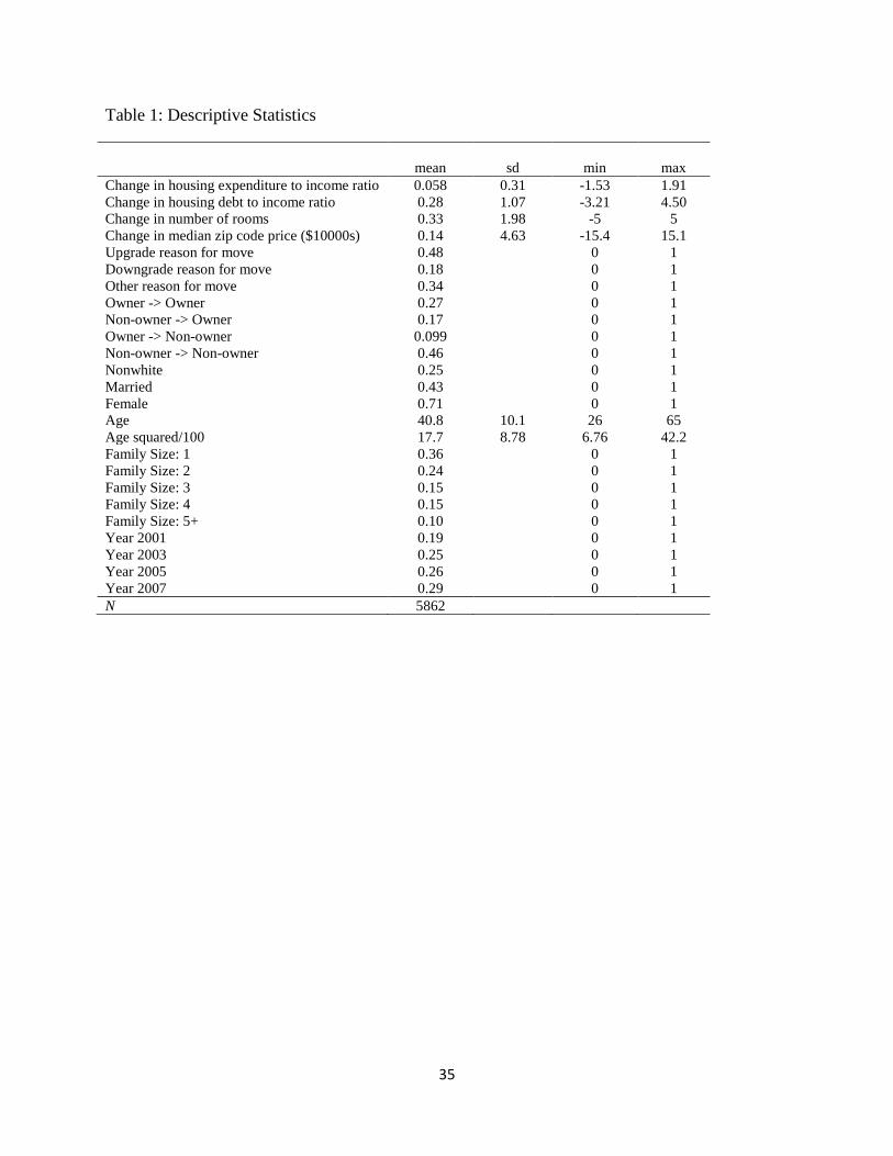
costs increased. Table 1 presents descriptive statistics for the PSID. There were 5862 moves during the

period. Upgrades make up 48% of these moves, downgrades are 18%, and other reasons make up the

remaining 34%. The percentage of moves in each two year period increased from 19% in 1999-2001 to

29% in 2007-2007. Even as prices were rising for housing, nearly half of the moves were made to

upgrade housing and as the bubble rose, more and more households felt compelled to move. Table 1

shows that 46% of the moves were for households going from one rental to another. Only 17% of the

moves reflected households moving from renting a home to buying one. 27% of the moves were for

owners who then moved on to own a new house while 10% were owners who sold their homes to become

renters.

(Table 1 here)

Figure 3 breaks out the types of moves by income groups. Here, one can see the income effects

on housing quite clearly. Around 65% of all moves by the bottom 50% of the income distribution was for

people moving from one rental to another. For the top income group, nearly 65% of the moves were for

21

people who were moving from owning one house to owning another. If one includes the people who went

from being renter to owners in this total, nearly 80% of the moves for the top income group were for

people who ended up owning homes. Conversely, only about 30% of all moves for people in the bottom

50% of the income distribution ended up with people owning homes. These differences are highly

statistically significant using a chi square test.

(Figure 3 about here)

Figure 4 shows the percent of moves that were upgrades, downgrades, or other across ownership

statuses. High income moves were predominantly for upgrading housing in the largest categories of

people moving from ownership to ownership or moving from rentals to ownership. Low income moves

were less likely to be upward in these categories. About 40% of the total moves by low income

households were downgrades while only 21% of high income households undertook downgrades. This is

consistent with hypothesis 1. Low income renters were more likely to upgrade than downgrade suggesting

that they were striving to get better housing even as rents and house prices were going up. This is contrary

to hypothesis 3. The middle income category experienced the largest amount of moves from not owning a

house to owning a house. This is evidence that middle class earners who were renters were buying homes

even as prices were rising and were the ones who experienced the most housing mobility.

(Figure 4about here)

Figure 4 presents data that shows the percentages within housing transition categories. The

different income groups were more or less the same likelihood to either move up or down if they managed

to shift hosing statuses. Most households who moved from owning one house to another, or from renting

to owning reported upgrading across income groups. Similarly, households that sold houses and returned

to being renters saw their moves as mostly downgrading. We take this evidence as suggesting that all

households who were able to move within ownership category were equally likely to improve their

22

housing situation even as house prices and rents were increasing. This is clear evidence that at every level

of income, households wanted to “keep up with the Joneses”.

(Figure 4 about here)

Our descriptive statistics provide confirmation of our overall story. Higher income groups did

upgrade more often and were likely to move from home ownership to home ownership. But we also see

evidence that once households had committed to moving, they were mostly improving their housing. This

implies that lower income households were more likely to be shut out of home ownership, but for those

who managed to buy a home, they upgraded at equal rates to higher income households.

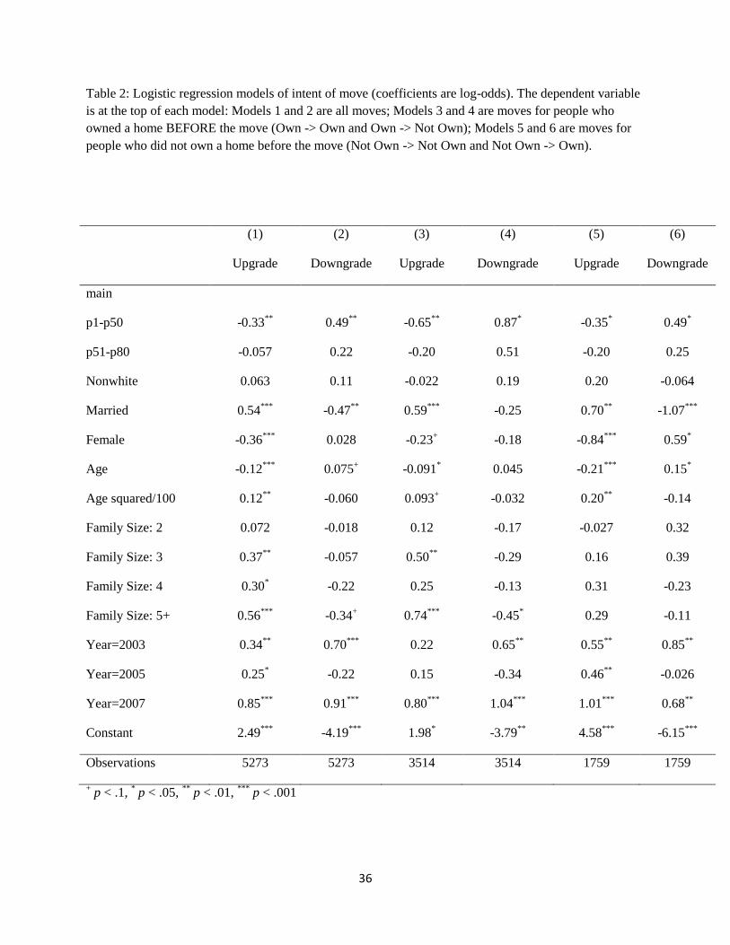
Table 2 models the determinants of who upgrades and who downgrades their housing. The first 2

models of the table model upward and downward moves for all moves. Here, we see clearly that low

income groups are less likely to upgrade their housing and more likely to downgrade their housing.

Married households and larger size households are more likely to upgrade than unmarried individuals or

female headed households and households with fewer members. This provides support for hypothesis 1.

These results are the same for households who start out owning a home (models 3-4) and for those who

start out renting (models 5-6). This provides support for hypotheses 2 and 3.

(Table 2 about here)

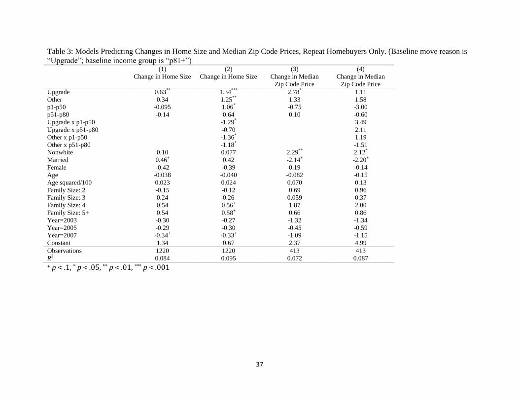
Table 3 considers the determinants of changes in house size and median zip code prices for

movers who are repeat homebuyers. Models 1 and 3 show that respondent’s reasons to move (i.e. to

upgrade or downgrade) were reflected in their choice of housing size and neighborhood costs. Households

who reported upgrading also reported increasing their house size by over a half a room and moved into

neighborhoods where house were almost $30,000 more expensive. This is for the first part of hypothesis

4. Models 2 and 4 examine the interaction between income and upgrading in order to evaluate if upper

income households are more likely to have larger changes in house size and median house price than low

income households. While there is some interaction between upgrading and income, the total effects are

23

not large. This implies that the main mechanism by which higher income effects housing consumption is

through the ability to upgrade housing by buying a bigger house in a more expensive neighborhood.

There are also no direct effects for being married or family size on moving to a larger house in a better

neighborhood. But there was evidence (Table 2) that being married and having more family members

was a determinant of upgrading housing. This provides partial support for hypothesis 7 at least for those

who could upgrade.

(Table 3 about here)

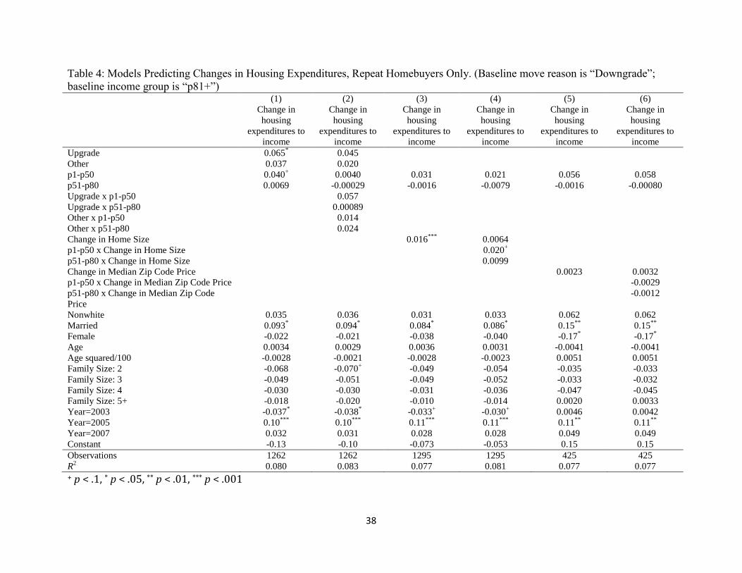
Table 4 models the changes in the ratio of housing expenditures to income (hereafter, “housing

expenditures”). In model 1 we examine the relationship between housing expenditures and type of move.

Upgrades do appear to add changes to housing expenditures. An average upgrade implies an 8 percent

increase in the percent of one’s income spent on housing. Other moves result in a 6 percentage point

increase. The only other measure that is statistically significant is being married. Here, being married

means that housing expenditures go up in moves. This is consistent with hypothesis 4.

(Table 4 about here)

In model 2, we add interaction terms between each income group and type of move. The

coefficient for the bottom income group is positive and significant (b = .061, p < .05). Here, we do

observe any relationship. In models 3 through 6 of Table 4 we examine the relationship between housing

expenditures and some of the dimensions along with households can upgrade or downgrade. Models 3-4

examine changes in home size. Each room change is associated with a 1.7 percentage point change (p <

.001) in housing expenditures in model 3. Model 4 includes interaction terms between change in house

size and income group. There are no statistically significant interactions between income and house size.

There is also no effect of changing zip codes on housing expenditures (models 5-6).

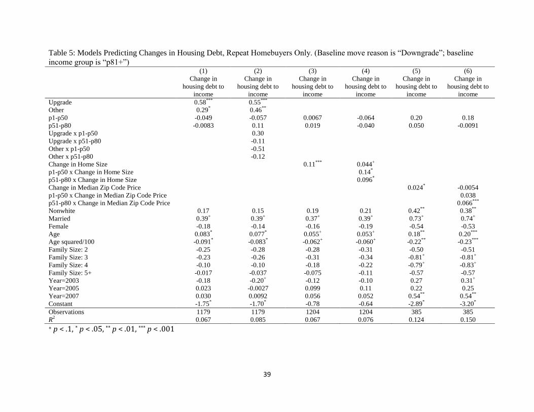
Table 5 presents results for the change in the ratio of mortgage debt to annual income (hereafter,

“housing debt”). Table5 presents the same independent variables as Table 4, but with housing debt as the

24

dependent variable. Model 1 shows that upgrades in housing result in significantly more housing debt

than downgrades and other moves. When we add interactions in model 2 between income and upgrades,

we find no statistically significant effects. Model 3 provides evidence that larger houses do raise housing

debt. When we add interactions terms with income (model 4), we find, that the effect of moving to a

larger home on housing debt is smallest for the highest earning households and largest for the lowest

earning households. Model 5 shows us that there is a significant effect of changes in median zip code

prices on housing debt. A $10,000 increase (decrease) in the median zip code is associated with a 2

percent increase (decrease) in the ratio of housing debt to income. Model 6 shows an interaction between

change in home size and change in median zip code price that was small and not statistically significant.

Again, this is evidence to support hypothesis 4.

Taken together, these results suggest that the main way that income effects changes in house size,

zip code valuations, house expenditures, and indebtedness are through households who already own

homes deciding to upgrade their housing. The highest income households who already own their housing

are the most likely to be able to upgrade while the lowest income households the least able to upgrade.

We have evidence that married households and households with children are more likely to upgrade while

single households and households headed by women are less likely to upgrade. When they choose to

upgrade, all households are likely to increase the size of their house, the quality of their zip code, their

housing expenses, and indebtedness.

(Table 5 about here)

We next focus on transitions in home ownership. For many households, becoming a homeowner

is an upgrade in itself. Of all moves, 17% were from being non-homeowners to homeowners. Of those

who became homeowners, 75% expressed an intention to upgrade as the reason for the move. Less than

6% called the move a downgrade. However, home ownership can be precarious as households depend

upon consistent income. Unemployment or other financial hardships force some households to downgrade

25

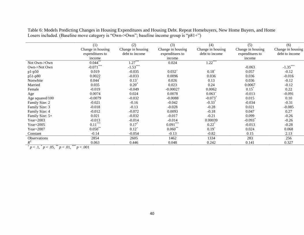
and no longer be homeowners. Ten percent of all moves are from owning to not owning. We examine

both transitions in both directions (Not own to own; own to not own) in Table 6. In these models we also

include as our baseline the “repeat homebuyers” households that owned homes both before and after the

move (that is, the households examined in the previous section). We let these repeat homebuyers be the

baseline category, to see how entering or leaving homeownership status affected households differently.

(Table 6 about here)

Model 1 of Table 6 models the change in the fraction of income spent on housing. Not

surprisingly, new homebuyers saw significant increases increase in housing expenditures compared to

repeat homebuyers (b = 0.044, p < .001). Households who lost their homes saw a significant decrease (b =

-0.071, p < .001). This is support for hypothesis 5. None of the other factors in the model were

statistically significant. Model 2 replaces housing expenditures with housing debt as the dependent

variable. We observe a significant increase in housing debt when one becomes a homeowner, and a

significant decrease when one sells one’s home. This is to be expected and support for hypothesis 5. New

homeowners do not have housing debt until they purchase home, while those who need to downgrade by

selling their home are, almost by definition, leaving behind the remaining debt on their homes.

Models 3 through 6 of Table 6 check the robustness of these results. In Models 4 and 5, we

compare only new homebuyers and repeat homebuyers who give an upgrade as a reason for the move. In

Models 5 and 6, we compare only home losers and repeat homebuyers who give a downgrade as a reason

for the move. Surprisingly, for households who move from renting to buying, the effect on housing

expenditures for being a new homebuyer compared to repeat homebuyers is still positive (Model 3), but

about half the size as in Model 1 and no longer significant. For housing debt (Model 4), the positive effect

for new homebuyers is about the same as in Model 2. For households who move from owners to renters,

there is no statistically significant difference in the change of housing expenditures between repeat

26

homebuyers and home losers, though the coefficient remains negative (Model 5). For housing debt

(Model 6), the negative effect for home losers is about the same as Model 2.

Renters make up 49% of all the moves in our data. Of these moves, households described 38% as

upgrades, 22% as downgrades, and 40% as other moves. However, the vast majority of these moves

(86%) are by movers in the bottom half of the income distribution. For this reason, in our analyses of non-

homeowners, we combine the middle and upper class households above the 50th percentile of the income

distribution. Table 7 models changes in home size and location price. In Model 1, we find that upward

moves do result in larger homes (b = 0.65, p < .001) supporting hypothesis 6. There are several other

significant effects. Female headed households tend to move to larger houses and increases in family size

also are related to having a larger house. Model 2 introduces interactions between income group and type

of move. None of these interactions are significant. Both gender of household head and the presence of

additional family members remain significant. Models 3 and 4 show how quality of area is associated

with moves. Again, our analysis here is restricted to only moves that involve a change in zip code for

which we have median price data on both zip codes. None of the coefficients is statistically significant.

This implies that renters, even those who are upgrading are neither inclined to move to more wealth off

areas, or more likely, the availability of rental housing is restricted in such areas. This suggests this [part

of hypothesis 6 is wrong.

(Table 7 about here)

Table 8 considers how changing locations affects renters housing expenditures. We note that

renters do not have mortgages so their change of moves cannot affect housing debt. Model 1 shows that

upgrading housing for renters has a statistically significant effect on their expenditures. There is also a

small effect for moving for other reasons on expenditures as well. The main other variable that is

statistically significant is nonwhite status. Here, nonwhites are less likely to increase their housing

expenditures when they move. In Model 2, we add interaction terms between each income group and type

27

of move. The main effect of upgrading on changes in housing expenditure appears to be for people in the

bottom 50% of the income distribution. This is consistent with hypothesis 6. The opportunity to upgrade

housing for the bottom half of the income distribution may not include buying a house. But if such

households can afford to upgrade, they will take on higher monthly expenditures on housing than higher

income households.

(Table 8 about here)

Models 3-4 add the effect of changing home size on housing expenditures. These models show

that getting a bigger house increases housing expenditures and does so in particular for lower income

households. Models 5-6 attempt to examine the link between moving to a higher priced zip code on

housing expenditures for renters. There is no main effect on such moves on housing costs. But, there is an

interaction with income group again. Here, renters in the bottom 50% who move to higher income

neighborhoods have higher changes in housing expenditures than higher income households.

Renters who moved who upgraded rented larger houses but not necessarily in nicer

neighborhoods (at least as measured by home prices). They also increased their housing expenses when

they upgraded. There is also evidence that renters were responding as much to pressures from family size

when they moved as they tended to move to larger and more expensive housing as family size grew.

Discussion and Conclusions

There are two interesting stories about status competition in our data analysis. The first

story is that income was the most important factor in determining whether or not households

were able to make housing moves that upgraded their housing situations in the housing bubble of

1999-2007. Not surprisingly, households in the top 20% of the income distribution were the most

28

likely to upgrade while households in the bottom 50% were the most likely to downgrade. But,

equally interesting is the evidence that households all through the income distribution did try to

improve their housing situations even as prices inflated through the period. Low income groups

who already owned homes and bought new ones were as likely to upgrade as high income

homeowners. Similarly, low income households who managed to move from renters to owners

upgraded their housing at a same rate as high income households. About 60% of the moves that

renters made (over 80% of whom were in the bottom 50% of the income distribution) were to

upgrade housing. Low income renters did not show a tendency to downgrade housing at a higher

rate than high income renters implying that they too were trying to keep up with the Joneses.

Our findings suggest that one way to think about the link between stratification and

housing is that there are three large income groups each of which is affected by rising house

prices in different ways. People in the bottom 50% of the income distribution were least likely to

buy homes and most likely to move as renters. As a result, their ability to attain the American

dream of owning a house was not fulfilled over this period. To the extent that they did

participate, the primary lifestyle struggle was to attain homeownership. Rising prices meant that

this came at the cost of considerable debt for those lower in the socio-economic hierarchy. When

they did buy, those in the bottom 50% went the most deeply into debt of any group. They tended

to buy those houses in less expensive zip codes and opted for larger houses and bigger debt loads

implying that the status competition for them was gaining a foothold into the American Dream.

Middle and upper middle class income groups (50-100%) faced a different kind of pressure.

They were able to buy and own houses. But, they too had to devote more of their expenditure to

housing and go ever-deeper into debt to do so.

29

Our results imply several lines of additional research. First, we think that the role of

children and schools in maintaining lifestyles bears further scrutiny. We have evidence that

family size was a predictor of housing upgrades net of income. It would be interesting to try and

explore whether or not such moves were to enter better school districts. One tactic could be to

incorporate data on school quality directly in order to see if households with children paid more

money for better schools. However, this data is complex to gather. For example, some school

districts are quite large (like in Los Angeles) and any measure of school quality is likely to mask

differences in house price increases for movers related to school quality. Moreover, many

parents at the top of the income distribution put their children into private schools.

Second, sociologists have been slow to unpack the linkages between income inequality,

indebtedness, housing, and place, for the social position of households. Our results, while

complex, show how place and housing play a big role in the social status of households.

Housing, place, and debt are not usually considered as stratification variables, but we have

shown how they play an important role in household’s social status and life styles.

Subsequent research should recognize that increasing income inequality affects

households quite differently given where they are place on the income distribution. Our results

support a sociological view of how growing income inequality dramatically affected household’s

ability to attain a middle life lifestyle during a time of rapid house price increases. Households

responded to those at the top bidding up house prices by taking on debt and increased monthly

expenditures to buy the best house they could. This created not only a middle class squeeze, but

an even more pronounced upper middle class squeeze. Life for households in the bottom 50% of

the income distribution became even harder as the ultimate status symbol of a middle class

30

lifestyle, owning a home, was difficult to attain and when purchased pushed households to the

highest levels of indebtedness.

31

Bibliography

Akerlof, George A., and Robert J. Shiller. 2010. Animal Spirits: How Human Psychology Drives

the Economy, and Why It Matters for Global Capitalism. Princeton, N.J.: Princeton

University Press.

Atkinson, Anthony, Thomas Picketty, and Emmanuel Saez. 2014. “Top incomes in the long run

of history.” Journal of Economic Literature 49: 3-71.

Barr, Michael. 2012. No Slack: The Financial Lives of Low-Income Americans. Washington,

D.C.: Brookings Institution Press, 2012.

Bertrand, Mary and Adair Morse. 2013. “Trickle Down Consumption.” NBER Working Paper

18883.

Black, Sandra. 1999. “Do Better Schools Matter? Parental Valuation of Elementary Education”.

The Quarterly Journal of Economics 114: 577-59.

Bourdieu, Pierre. 1984. Distinctions. Cambridge, Ma.: Harvard University Press.

Bruce, Andrew. 2014. “Zillow Home Value Index: Methodology” Zillow Real Estate Research.

Retrieved Aug. 15, 2014. (http://www.zillow.com/research/zhvi-methodology-6032/).

Charles, Maria and Lundy, Jeff. 2012. "The Local Joneses: Household Consumption and Income

Inequality in Large Metropolitan Areas." Paper presented at the annual meeting of the

American Sociological Association Annual Meeting, Denver, CO, Aug 16, 2012.

Clapp, John A., Anupam Nanda, and Stephen L. Ross. 2008. “Which school attributes

matter?:The influence of school district performance and demographic composition on

property values.” Journal of Urban Economics 63: 451–466.

Cynamon, Barry and Steven Fazzari. 2009. “Household debt in the consumer age: source of

growth – risk of collapse.” Comparative Economic and Social Systems, 3:49-55.

Dupuis, Ann and David Thorns. 2002. “Home, home ownership and the search for ontological

security.” The Sociological Review, 46, 24-47.

Dwyer, Rachel E. 2009. “The McMansionization of America? Income Stratification and the

Standard of Living in Housing, 1960-2000.” Research in Social Stratification and

Mobility 27: 285-300.

Dynan, Karen E., and Donald L. Kohn. 2007. “The Rise in U.S. Household Indebtedness: Causes

and Consequences.” Finance and Economics Discussion Series No. 2007-37. Divisions of

Research & Statistics and Monetary Affairs. Federal Reserve Board, Washington, D.C.

Elias, Norbert. 1994. The Civilizing Process. Oxford, Eng.: Blackwell Press.

32

Erturk, Ismail, Julie Froud, Sukhdev Johal, Adam Leaver and Karel Williams. 2007. 'The

democratization of finance? Promises, outcomes and conditions,’ Review of International

Political Economy, 14 (4): 197-216.

Fligstein, Neil and Taekjin Shin. 2004. “The shareholder value society: a review of the changes in

working conditions and inequality in the United States, 1976-2000.” In Kathryn

Neckerman (ed.) The New Inequalities. New York: Russell Sage Foundation.

___________ and Zawadi Rucks Ahidiana. 2014. “The rich stay richer: the effects on the 2007-

2009 financial crisis on household welfare”. Paper presented at the Thematic Session on

“Institutions and Inequality” at the 2014 Annual Meetings of the American Sociological

Association, San Francisco, Ca., August 16-19, 2014.

___________ and Adam Goldstein. Forthcoming. “The emergence of a finance culture in

American households, 1989-2007”. Socio-Economic Review, forthcoming.

Frank, Robert. 1989.”Frames of Reference and the Quality of Life.” American Economic Review.

79(2): 80-85. Papers and Proceedings of the Hundred and First Annual Meeting of the

American Economic Association.

___________. 2007a. “Does Context Matter More for Some Goods than Others?” in Marina

Bianchi (ed.) The Evolution of Consumption: Theories and Practices (Advances in

Austrian Economics, Volume 10) Emerald Group Publishing Limited, pp.231 – 248.

____________. 2007b. Falling Behind: How Rising Inequality Harms the Middle Class. Berkeley,

Ca.: University of California Press.

Goldstein, Adam. 2012. “Income, consumption, and household indebtedness in the U.S., 1989-

2007”. Department of Sociology, University of California. Unpublished Manuscript.

Hacker, Jacob. 2006. The Great Risk Shift. New York: Oxford University Press.

Hirsch, Fred. 1977. The Social Limits to Growth. London: Routledge & Kegan Paul.

Hyman, Louis. 2011. Debtor Nation: A History of America in Red Ink. Princeton, N.J.: Princeton

University Press.

Kalleberg, Arne. 2009. “Precarious work, insecure workers: Employment relations in transition.”

American Sociological Review 74:1–22.

manning

Langley, Paul. 2008. The Everyday fe of Global Finance: Saving and Borrowing in Anglo-

America. Oxford University Press.

Leicht, Kevin and Scott Fitzgerald. 2006. Post-Industrial Peasants. Macmillan Press.

33

Levine, Adam, Robert H. Frank, and Oege Dijk. 2010. “Expenditure Cascades.” (working paper).

pp. 1-34. http://papers.ssrn.com/sol3/papers.cfm?abstract_id=1690612.

Li, Geng, Robert Schoeni, Sheldon Danziger, and Kerwin Charles. 2010. "New Expenditure

Data in the Panel Study of Income Dynamics: Comparisons with the Consumer

Expenditure Survey Data." Monthly Labor Review: 29-39.

Manning, Robert D. 2001. Credit Card Nation. New York: Basic Books.

Matlack, Janna L., and Jacob L. Vigdor. 2008. "Do rising tides lift all prices? Income inequality

and housing affordability." Journal of Housing Economics 17.3: 212-224.

McCloud, Laura and Rachel Dwyer. 2011. “The fragile American: Hardship and Financial

Troubles in the 21st century.” The Sociological Quarterly 52:13-35.

Megbolugbe, Isaac and Peter D . Linneman. 1993. “Home ownership.” Urban Studies 30: 659-

682.

Mian, Atif and Sufi, Amir. 2014. House of Debt. Chicago, Il: University of Chicago Press.

Panel Study of Income Dynamics, restricted use dataset. Produced and distributed by the Survey

Research Center, Institute for Social Research, University of Michigan, Ann Arbor, MI

(data downloaded in 2014).

Pew Research Center. 2008. Inside the Middle Class: Bad Times Hit the Good Life. Pew

Research Center Trends Report, April 9, 2008.

Porter, Katherine. 2012. Broke: How Debt Bankrupts the Middle Class. Stanford, Ca.: Stanford

University Press.

Rajan, Raghuram. 2010. Fault Lines: How Hidden Fractures Still Threaten the World Economy.

Princeton, N.J.: Princeton University Press.

Rivera L. and Lamont M. 2012. “Price vs. Pets, Schools vs. Styles: The Residential Priorities of

the American Upper-Middle Class”. Paper presented at the 2012 meeting of the Eastern

Sociological Society, New York City.

Savage, Howard A. 2009 "Who could afford to buy a home in 2004?" US Census Bureau.

Schor, Juliet. 1998. The Overspent American. New York: Basic Books.

Shiller, Robert. 2008. “Understanding recent trends in house prices and home ownership. “ NBER

Working paper 13553. Cambridge, Ma.: National Bureau of Economic Research.

Schwartz, Mary, and Ellen Wilson. 2008. "Who Can Afford To Live in a Home?: A look at data

from the 2006 American Community Survey." US Census Bureau.

34

Sobel, Michael. 1981. Lifestyle and Social Structure. New York: Academic Press.

Trumbull, Gerald. 2012. “Credit access and social welfare: The rise of consumer lending in the

United States and France.” Politics & Society 40 (1) (March 1): 9–34.

U.S. Bureau of the Census. 2011. “House size over time.” Accessed on August 26, 2014 at

http://www.census.gov/const/C25Ann/sftotalmedavgsqft.pdf.

Weber, Max. 1946. From Max Weber: Essays in Sociology. Edited by Hans Gerth and C. Wright

Mills. New York: Oxford University Press.

Western, Bruce, Deidre Bloome, Benjamin Sosnaud, and Laura Tauch. 2012. “Economic

insecurity and social stratification.” Annual Review of Sociology 38:341-359.

Zillow Real Estate Research. 2014. “Home Value Index.” Machine-readable Data File.

(http://files.zillowstatic.com/research/public/County/County_Zhvi_AllHomes.csv)

35

Table 1: Descriptive Statistics

mean sd min max

Change in housing expenditure to income ratio 0.058 0.31 -1.53 1.91

Change in housing debt to income ratio 0.28 1.07 -3.21 4.50

Change in number of rooms 0.33 1.98 -5 5

Change in median zip code price ($10000s) 0.14 4.63 -15.4 15.1

Upgrade reason for move 0.48 0 1

Downgrade reason for move 0.18 0 1

Other reason for move 0.34 0 1

Owner -> Owner 0.27 0 1

Non-owner -> Owner 0.17 0 1

Owner -> Non-owner 0.099 0 1

Non-owner -> Non-owner 0.46 0 1

Nonwhite 0.25 0 1

Married 0.43 0 1

Female 0.71 0 1

Age 40.8 10.1 26 65

Age squared/100 17.7 8.78 6.76 42.2

Family Size: 1 0.36 0 1

Family Size: 2 0.24 0 1

Family Size: 3 0.15 0 1

Family Size: 4 0.15 0 1

Family Size: 5+ 0.10 0 1

Year 2001 0.19 0 1

Year 2003 0.25 0 1

Year 2005 0.26 0 1

Year 2007 0.29 0 1

N 5862

36

Table 2: Logistic regression models of intent of move (coefficients are log-odds). The dependent variable

is at the top of each model: Models 1 and 2 are all moves; Models 3 and 4 are moves for people who

owned a home BEFORE the move (Own -> Own and Own -> Not Own); Models 5 and 6 are moves for

people who did not own a home before the move (Not Own -> Not Own and Not Own -> Own).

(1) (2) (3) (4) (5) (6)

Upgrade Downgrade Upgrade Downgrade Upgrade Downgrade

main

p1-p50 -0.33**

0.49**

-0.65**

0.87* -0.35

* 0.49

*

p51-p80 -0.057 0.22 -0.20 0.51 -0.20 0.25

Nonwhite 0.063 0.11 -0.022 0.19 0.20 -0.064

Married 0.54***

-0.47**

0.59***

-0.25 0.70**

-1.07***

Female -0.36***

0.028 -0.23+ -0.18 -0.84

*** 0.59

*

Age -0.12***

0.075+ -0.091

* 0.045 -0.21

*** 0.15

*

Age squared/100 0.12**

-0.060 0.093+ -0.032 0.20

** -0.14

Family Size: 2 0.072 -0.018 0.12 -0.17 -0.027 0.32

Family Size: 3 0.37**

-0.057 0.50**

-0.29 0.16 0.39

Family Size: 4 0.30* -0.22 0.25 -0.13 0.31 -0.23

Family Size: 5+ 0.56***

-0.34+ 0.74

*** -0.45

* 0.29 -0.11

Year=2003 0.34**

0.70***

0.22 0.65**

0.55**

0.85**

Year=2005 0.25* -0.22 0.15 -0.34 0.46

** -0.026

Year=2007 0.85***

0.91***

0.80***

1.04***

1.01***

0.68**

Constant 2.49***

-4.19***

1.98* -3.79

** 4.58

*** -6.15

***

Observations 5273 5273 3514 3514 1759 1759

+ p < .1,

* p < .05,

** p < .01,

*** p < .001

37

Table 3: Models Predicting Changes in Home Size and Median Zip Code Prices, Repeat Homebuyers Only. (Baseline move reason is

“Upgrade”; baseline income group is “p81+”) (1) (2) (3) (4)

Change in Home Size Change in Home Size Change in Median

Zip Code Price

Change in Median

Zip Code Price

Upgrade 0.63**

1.34***

2.78* 1.11

Other 0.34 1.25**

1.33 1.58

p1-p50 -0.095 1.06* -0.75 -3.00

p51-p80 -0.14 0.64 0.10 -0.60

Upgrade x p1-p50 -1.29* 3.49

Upgrade x p51-p80 -0.70 2.11

Other x p1-p50 -1.36* 1.19

Other x p51-p80 -1.18* -1.51

Nonwhite 0.10 0.077 2.29**

2.12*

Married 0.46+ 0.42 -2.14

+ -2.20

+

Female -0.42 -0.39 0.19 -0.14

Age -0.038 -0.040 -0.082 -0.15

Age squared/100 0.023 0.024 0.070 0.13

Family Size: 2 -0.15 -0.12 0.69 0.96

Family Size: 3 0.24 0.26 0.059 0.37

Family Size: 4 0.54 0.56+ 1.87 2.00

Family Size: 5+ 0.54 0.58+ 0.66 0.86

Year=2003 -0.30 -0.27 -1.32 -1.34

Year=2005 -0.29 -0.30 -0.45 -0.59

Year=2007 -0.34+ -0.33

+ -1.09 -1.15

Constant 1.34 0.67 2.37 4.99

Observations 1220 1220 413 413

R2 0.084 0.095 0.072 0.087

+ p < .1, * p < .05, ** p < .01, *** p < .001

38

Table 4: Models Predicting Changes in Housing Expenditures, Repeat Homebuyers Only. (Baseline move reason is “Downgrade”;

baseline income group is “p81+”) (1) (2) (3) (4) (5) (6)

Change in

housing

expenditures to

income

Change in

housing

expenditures to

income

Change in

housing

expenditures to

income

Change in

housing

expenditures to

income

Change in

housing

expenditures to

income

Change in

housing

expenditures to

income

Upgrade 0.065* 0.045

Other 0.037 0.020

p1-p50 0.040+ 0.0040 0.031 0.021 0.056 0.058

p51-p80 0.0069 -0.00029 -0.0016 -0.0079 -0.0016 -0.00080

Upgrade x p1-p50 0.057

Upgrade x p51-p80 0.00089

Other x p1-p50 0.014

Other x p51-p80 0.024

Change in Home Size 0.016***

0.0064

p1-p50 x Change in Home Size 0.020+

p51-p80 x Change in Home Size 0.0099

Change in Median Zip Code Price 0.0023 0.0032

p1-p50 x Change in Median Zip Code Price -0.0029

p51-p80 x Change in Median Zip Code

Price

-0.0012

Nonwhite 0.035 0.036 0.031 0.033 0.062 0.062

Married 0.093* 0.094

* 0.084

* 0.086

* 0.15

** 0.15

**

Female -0.022 -0.021 -0.038 -0.040 -0.17* -0.17

*

Age 0.0034 0.0029 0.0036 0.0031 -0.0041 -0.0041

Age squared/100 -0.0028 -0.0021 -0.0028 -0.0023 0.0051 0.0051

Family Size: 2 -0.068 -0.070+ -0.049 -0.054 -0.035 -0.033

Family Size: 3 -0.049 -0.051 -0.049 -0.052 -0.033 -0.032

Family Size: 4 -0.030 -0.030 -0.031 -0.036 -0.047 -0.045

Family Size: 5+ -0.018 -0.020 -0.010 -0.014 0.0020 0.0033

Year=2003 -0.037* -0.038

* -0.033

+ -0.030

+ 0.0046 0.0042

Year=2005 0.10***

0.10***

0.11***

0.11***

0.11**

0.11**

Year=2007 0.032 0.031 0.028 0.028 0.049 0.049

Constant -0.13 -0.10 -0.073 -0.053 0.15 0.15

Observations 1262 1262 1295 1295 425 425

R2 0.080 0.083 0.077 0.081 0.077 0.077

+ p < .1, * p < .05, ** p < .01, *** p < .001

39

Table 5: Models Predicting Changes in Housing Debt, Repeat Homebuyers Only. (Baseline move reason is “Downgrade”; baseline

income group is “p81+”) (1) (2) (3) (4) (5) (6)

Change in

housing debt to

income

Change in

housing debt to

income

Change in

housing debt to

income

Change in

housing debt to

income

Change in

housing debt to

income

Change in

housing debt to

income

Upgrade 0.58***

0.55***

Other 0.29* 0.46

**

p1-p50 -0.049 -0.057 0.0067 -0.064 0.20 0.18

p51-p80 -0.0083 0.11 0.019 -0.040 0.050 -0.0091

Upgrade x p1-p50 0.30

Upgrade x p51-p80 -0.11

Other x p1-p50 -0.51

Other x p51-p80 -0.12

Change in Home Size 0.11***

0.044+

p1-p50 x Change in Home Size 0.14*

p51-p80 x Change in Home Size 0.096*

Change in Median Zip Code Price 0.024* -0.0054

p1-p50 x Change in Median Zip Code Price 0.038

p51-p80 x Change in Median Zip Code Price 0.066***

Nonwhite 0.17 0.15 0.19 0.21 0.42**

0.38**

Married 0.39+ 0.39

+ 0.37

+ 0.39

+ 0.73

+ 0.74

+

Female -0.18 -0.14 -0.16 -0.19 -0.54 -0.53

Age 0.083* 0.077

* 0.055

+ 0.053

+ 0.18

** 0.20

***

Age squared/100 -0.091* -0.083

* -0.062

+ -0.060

+ -0.22

** -0.23

***

Family Size: 2 -0.25 -0.28 -0.28 -0.31 -0.50 -0.51

Family Size: 3 -0.23 -0.26 -0.31 -0.34 -0.81+ -0.81

+

Family Size: 4 -0.10 -0.10 -0.18 -0.22 -0.79+ -0.83

+

Family Size: 5+ -0.017 -0.037 -0.075 -0.11 -0.57 -0.57

Year=2003 -0.18 -0.20+ -0.12 -0.10 0.27 0.31

+

Year=2005 0.023 -0.0027 0.099 0.11 0.22 0.25

Year=2007 0.030 0.0092 0.056 0.052 0.54**

0.54**

Constant -1.75* -1.70

* -0.78 -0.64 -2.89

* -3.20

*

Observations 1179 1179 1204 1204 385 385

R2 0.067 0.085 0.067 0.076 0.124 0.150

+ p < .1, * p < .05, ** p < .01, *** p < .001

40

Table 6: Models Predicting Changes in Housing Expenditures and Housing Debt. Repeat Homebuyers, New Home Buyers, and Home

Losers included. (Baseline move category is “Own->Own”; baseline income group is “p81+”)

(1) (2) (3) (4) (5) (6)

Change in housing

expenditures to

income

Change in housing

debt to income

Change in housing

expenditures to

income

Change in housing

debt to income

Change in housing

expenditures to

income

Change in housing

debt to income

Not Own->Own 0.044**

1.27***

0.024 1.22***

Own->Not Own -0.071***

-1.53***

-0.063 -1.35***

p1-p50 0.019 -0.035 0.032+ 0.18

+ 0.057 -0.12

p51-p80 0.0022 -0.033 0.0096 0.036 0.036 -0.016

Nonwhite 0.044* 0.13

+ 0.026 0.13 0.036 -0.12

Married 0.035 0.20* 0.023 0.24 0.0067 -0.12

Female -0.019 -0.049 -0.00027 0.0062 0.15* 0.22

Age 0.0074 0.024 0.0078 0.063+ -0.013 -0.091

Age squared/100 -0.0079 -0.032 -0.0088 -0.073+ 0.015 0.10

Family Size: 2 -0.021 -0.16 -0.042 -0.33* -0.034 -0.31

Family Size: 3 -0.018 -0.13 -0.028 -0.28 0.021 -0.085

Family Size: 4 -0.012 -0.072 0.0093 -0.18 0.047 0.27

Family Size: 5+ 0.021 -0.032 -0.017 -0.21 0.099 -0.26

Year=2003 -0.013 -0.014 -0.014 0.00039 -0.093* -0.26

Year=2005 0.11***

0.17* 0.091

*** 0.22

* -0.013 -0.28

Year=2007 0.050**

0.12+ 0.060

** 0.19

+ 0.024 0.068

Constant -0.14 -0.054 -0.13 -0.82 0.15 2.13

Observations 2854 2605 1462 1334 283 256

R2 0.063 0.446 0.048 0.242 0.141 0.327

+ p < .1,

* p < .05,

** p < .01,

*** p < .001

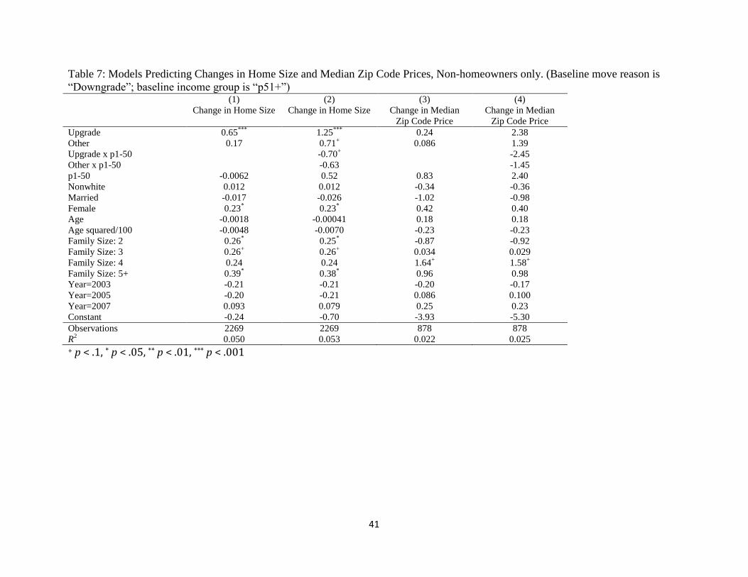
41

Table 7: Models Predicting Changes in Home Size and Median Zip Code Prices, Non-homeowners only. (Baseline move reason is

“Downgrade”; baseline income group is “p51+”) (1) (2) (3) (4)

Change in Home Size Change in Home Size Change in Median

Zip Code Price

Change in Median

Zip Code Price

Upgrade 0.65***

1.25***

0.24 2.38

Other 0.17 0.71+ 0.086 1.39

Upgrade x p1-50 -0.70+ -2.45

Other x p1-50 -0.63 -1.45

p1-50 -0.0062 0.52 0.83 2.40

Nonwhite 0.012 0.012 -0.34 -0.36

Married -0.017 -0.026 -1.02 -0.98

Female 0.23* 0.23

* 0.42 0.40

Age -0.0018 -0.00041 0.18 0.18

Age squared/100 -0.0048 -0.0070 -0.23 -0.23

Family Size: 2 0.26* 0.25

* -0.87 -0.92

Family Size: 3 0.26+ 0.26

+ 0.034 0.029

Family Size: 4 0.24 0.24 1.64+ 1.58

+

Family Size: 5+ 0.39* 0.38

* 0.96 0.98

Year=2003 -0.21 -0.21 -0.20 -0.17

Year=2005 -0.20 -0.21 0.086 0.100

Year=2007 0.093 0.079 0.25 0.23

Constant -0.24 -0.70 -3.93 -5.30

Observations 2269 2269 878 878

R2 0.050 0.053 0.022 0.025

+ p < .1, * p < .05, ** p < .01, *** p < .001

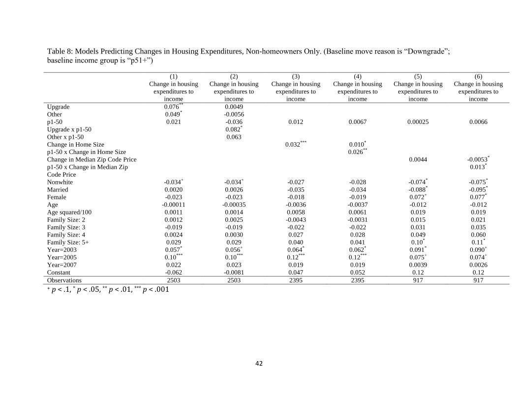
42

Table 8: Models Predicting Changes in Housing Expenditures, Non-homeowners Only. (Baseline move reason is “Downgrade”;

baseline income group is “p51+”)

(1) (2) (3) (4) (5) (6)

Change in housing

expenditures to

income

Change in housing

expenditures to

income

Change in housing

expenditures to

income

Change in housing

expenditures to

income

Change in housing

expenditures to

income

Change in housing

expenditures to

income

Upgrade 0.076**

0.0049

Other 0.049* -0.0056

p1-50 0.021 -0.036 0.012 0.0067 0.00025 0.0066

Upgrade x p1-50 0.082*

Other x p1-50 0.063

Change in Home Size 0.032***

0.010*

p1-50 x Change in Home Size 0.026**

Change in Median Zip Code Price 0.0044 -0.0053*

p1-50 x Change in Median Zip

Code Price

0.013*

Nonwhite -0.034+ -0.034

+ -0.027 -0.028 -0.074

* -0.075

*

Married 0.0020 0.0026 -0.035 -0.034 -0.088* -0.095

*

Female -0.023 -0.023 -0.018 -0.019 0.072+ 0.077

*

Age -0.00011 -0.00035 -0.0036 -0.0037 -0.012 -0.012

Age squared/100 0.0011 0.0014 0.0058 0.0061 0.019 0.019

Family Size: 2 0.0012 0.0025 -0.0043 -0.0031 0.015 0.021

Family Size: 3 -0.019 -0.019 -0.022 -0.022 0.031 0.035

Family Size: 4 0.0024 0.0030 0.027 0.028 0.049 0.060

Family Size: 5+ 0.029 0.029 0.040 0.041 0.10* 0.11

*

Year=2003 0.057* 0.056

+ 0.064

* 0.062

* 0.091

* 0.090

+

Year=2005 0.10***

0.10***

0.12***

0.12***

0.075+ 0.074

+

Year=2007 0.022 0.023 0.019 0.019 0.0039 0.0026

Constant -0.062 -0.0081 0.047 0.052 0.12 0.12

Observations 2503 2503 2395 2395 917 917

+ p < .1, * p < .05, ** p < .01, *** p < .001

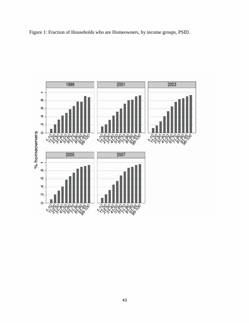
43

Figure 1: Fraction of Households who are Homeowners, by income groups, PSID.

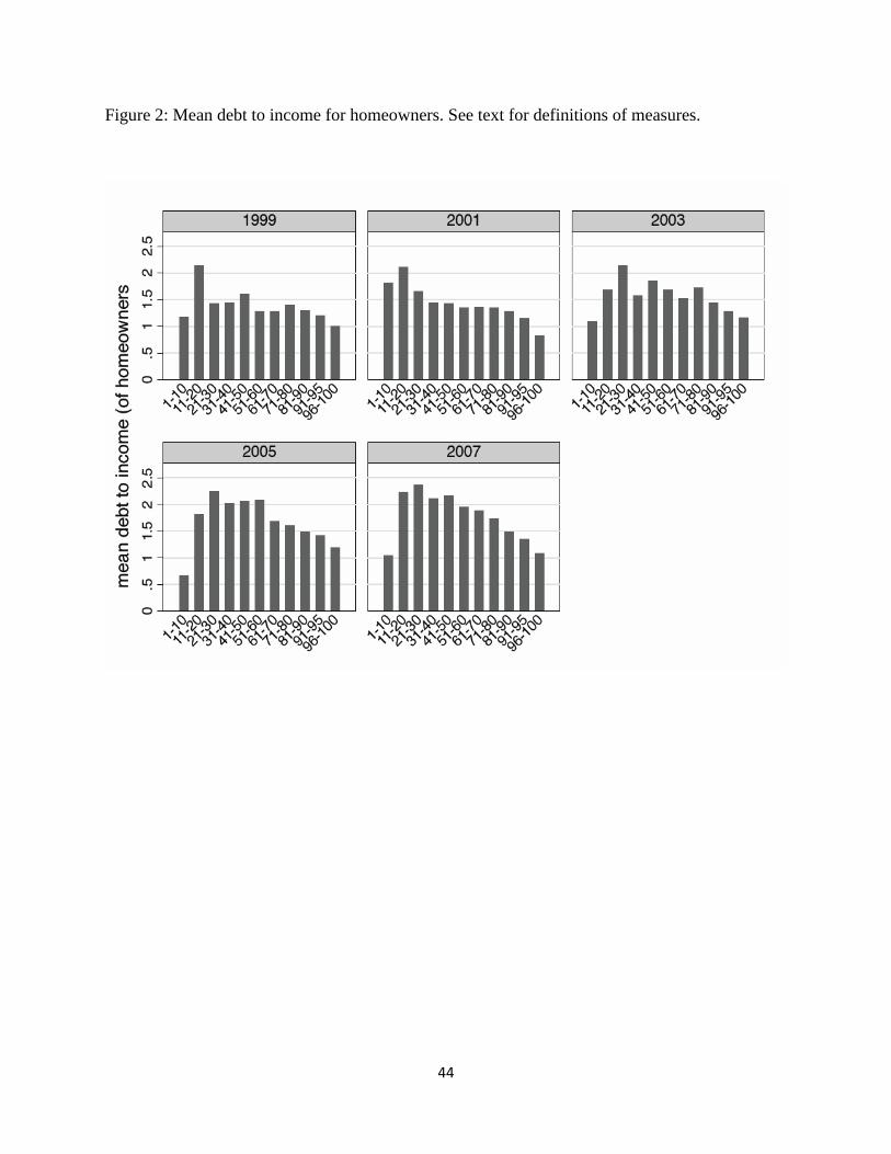
44

Figure 2: Mean debt to income for homeowners. See text for definitions of measures.

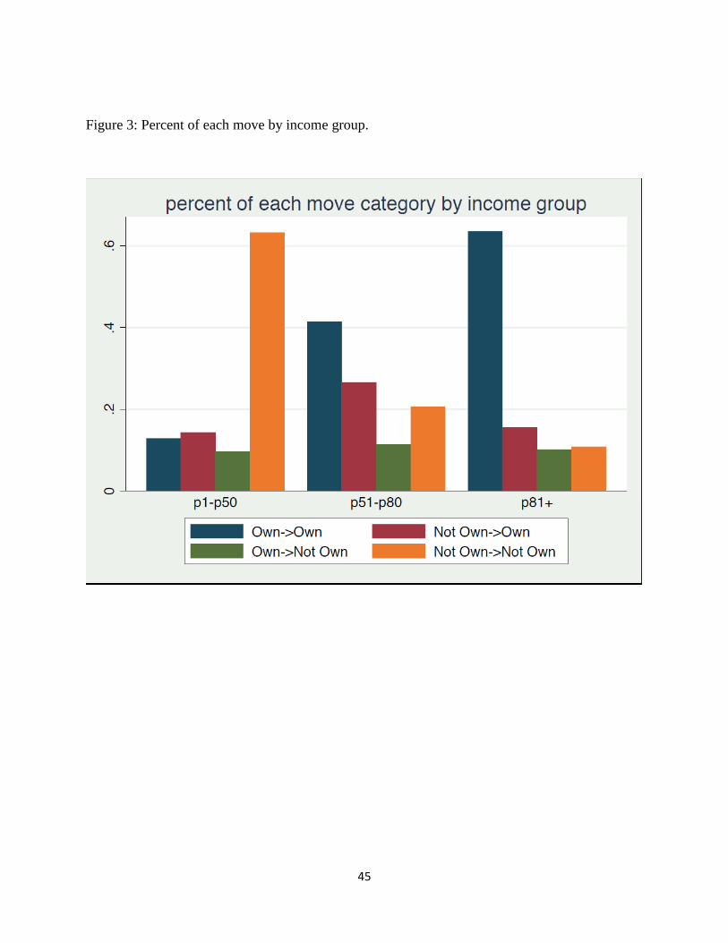
45

Figure 3: Percent of each move by income group.

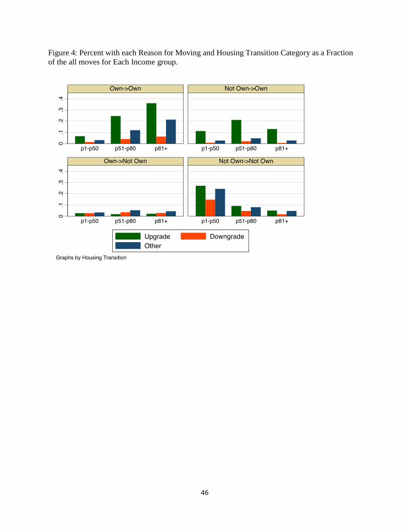
46

Figure 4: Percent with each Reason for Moving and Housing Transition Category as a Fraction

of the all moves for Each Income group.

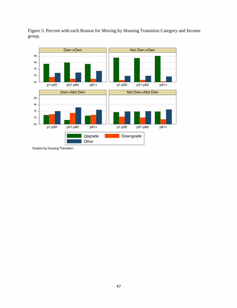
47

Figure 5: Percent with each Reason for Moving by Housing Transition Category and Income

group.