Investigations on Slug Flow in a Horizontal Pipe Using

INVESTIGATIONS ON SLUG FLOW IN A HORIZONTAL PIPE USING

STEREOSCOPIC PARTICLE IMAGE VELOCIMETRY AND CFD SIMULATION WITH VOLUME OF FLUID METHOD

Marek Czapp 1, Matthias Utschick 1, Johannes Rutzmoser 2, Thomas Sattelmayer 1

1: Chair of Thermodynamics, 2: Institute of Applied Mechanics

Technische Universität München Boltzmannstraße 15

85487 Garching near Munich (Germany) [email protected]

ABSTRACT Investigations on gas-liquid flows in horizontal pipes are of immanent importance for Reactor Safety Research. In case of a breakage of the main cooling circuit of a Pressurized Water Reactor (PWR), the pressure losses of the gas-liquid flow significantly govern the loss of coolant rate. The flow regime is largely determined by liquid and gas superficial velocities and contains slug flow that causes high-pressure pulsations to the infrastructure of the main cooling circuit. Experimental and numerical investigations on adiabatic slug flow of a water-air system were carried out in a horizontal pipe of about 10 m length and 54 mm diameter at atmospheric pressure and room temperature. Stereoscopic high-speed Particle Image Velocimetry in combination with Laser Induced Fluorescence was successfully applied on round pipe geometry to determine instantaneous three-dimensional water velocity fields of slug flows. After grid independence studies, numerical simulations were run with the open-source CFD program OpenFOAM. The solver uses the VOF method (Volume of Fluid) with phase-fraction interface capturing approach based on interface compression. It provides mesh refinement at the interfacial area to improve resolution of the interface between the two phases. Furthermore, standard k-� turbulence model was applied in an unsteady Reynolds averaged Navier Stokes (URANS) model to resolve self-induced slug formation. The aim of this work is to present the feasibility of both relatively novel possibilities of determining two-phase slug flows in pipes. Experimental and numerical results allow the comparison of the slug initiation and expansion process with respect to their axial velocities and cross-sectional void fractions.

INTRODUCTION Two-phase slug flow of liquid-gas mixtures may appear in many industrial applications, such as cooling systems of pressurized nuclear reactors, oil pipelines, or even turbines and are therefore of particular importance for industry. Efforts in developing and improving measurement techniques as well as optimization of existing CFD models for slug flow simulations are highly requested. The modeling of gas-liquid flow in horizontal pipes is especially in Reactor Safety Analysis (loss-of-coolant accident, LOCA) of considerable importance. Due to high pressure pulsations in slug flows, it is essential to understand and model this kind of flow in context of safety-related analysis. For instance, a transition from vertical to horizontal two-phase flow due to an elbow may lead to centrifugal separation, forming stratified flow in a certain part of the horizontal pipe, where transition from stratified to slug flow may be established. In case of slug flow, high pressure pulsations will affect the infrastructure of the main cooling circuit. The pressure losses depend on the flow regime, which is largely determined by the steam mass fraction and the superficial velocities. NOMENCLATURE Latin Letters c [ - ] Constant D [m] Diameter I [ - ] Unit matrix k [m2/s2] Kinetic energy L [m] Pipe length Re [ - ] Reynolds number t [ s ] Time v [m/s] Total velocity w [m/s] Axial velocity x,y, z [m] Cartesian axis directions

1 Copyright © 2012 by ASME

Proceedings of the 2012 20th International Conference on Nuclear Engineering collocated with the

ASME 2012 Power Conference ICONE20-POWER2012

July 30 - August 3, 2012, Anaheim, California, USA

ICONE20-POWER2012-54591

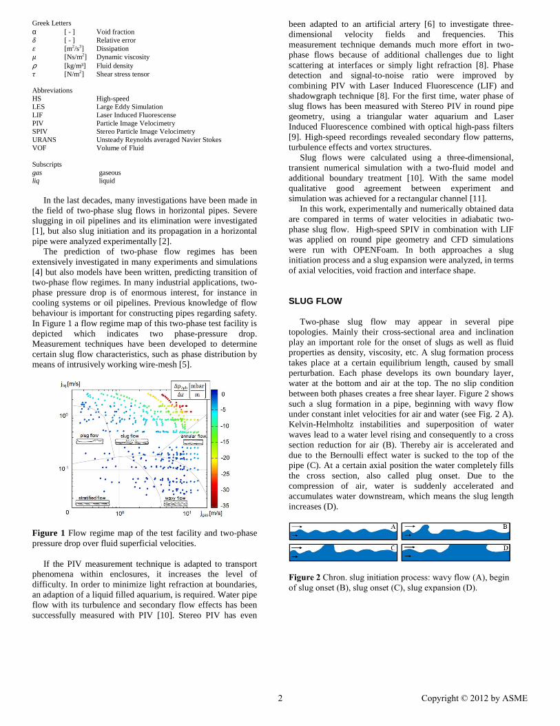
Greek Letters α [ - ] Void fraction � [ - ] Relative error � [m2/s3] Dissipation � [Ns/m2] Dynamic viscosity ρ [kg/m³] Fluid density � [N/m2] Shear stress tensor Abbreviations HS High-speed LES Large Eddy Simulation LIF Laser Induced Fluorescense PIV Particle Image Velocimetry SPIV Stereo Particle Image Velocimetry URANS Unsteady Reynolds averaged Navier Stokes VOF Volume of Fluid Subscripts gas gaseous liq liquid In the last decades, many investigations have been made in the field of two-phase slug flows in horizontal pipes. Severe slugging in oil pipelines and its elimination were investigated [1], but also slug initiation and its propagation in a horizontal pipe were analyzed experimentally [2]. The prediction of two-phase flow regimes has been extensively investigated in many experiments and simulations [4] but also models have been written, predicting transition of two-phase flow regimes. In many industrial applications, two-phase pressure drop is of enormous interest, for instance in cooling systems or oil pipelines. Previous knowledge of flow behaviour is important for constructing pipes regarding safety. In Figure 1 a flow regime map of this two-phase test facility is depicted which indicates two phase-pressure drop. Measurement techniques have been developed to determine certain slug flow characteristics, such as phase distribution by means of intrusively working wire-mesh [5].

Figure 1 Flow regime map of the test facility and two-phase pressure drop over fluid superficial velocities. If the PIV measurement technique is adapted to transport phenomena within enclosures, it increases the level of difficulty. In order to minimize light refraction at boundaries, an adaption of a liquid filled aquarium, is required. Water pipe flow with its turbulence and secondary flow effects has been successfully measured with PIV [10]. Stereo PIV has even

been adapted to an artificial artery [6] to investigate three-dimensional velocity fields and frequencies. This measurement technique demands much more effort in two-phase flows because of additional challenges due to light scattering at interfaces or simply light refraction [8]. Phase detection and signal-to-noise ratio were improved by combining PIV with Laser Induced Fluorescence (LIF) and shadowgraph technique [8]. For the first time, water phase of slug flows has been measured with Stereo PIV in round pipe geometry, using a triangular water aquarium and Laser Induced Fluorescence combined with optical high-pass filters [9]. High-speed recordings revealed secondary flow patterns, turbulence effects and vortex structures. Slug flows were calculated using a three-dimensional, transient numerical simulation with a two-fluid model and additional boundary treatment [10]. With the same model qualitative good agreement between experiment and simulation was achieved for a rectangular channel [11]. In this work, experimentally and numerically obtained data are compared in terms of water velocities in adiabatic two-phase slug flow. High-speed SPIV in combination with LIF was applied on round pipe geometry and CFD simulations were run with OPENFoam. In both approaches a slug initiation process and a slug expansion were analyzed, in terms of axial velocities, void fraction and interface shape. SLUG FLOW Two-phase slug flow may appear in several pipe topologies. Mainly their cross-sectional area and inclination play an important role for the onset of slugs as well as fluid properties as density, viscosity, etc. A slug formation process takes place at a certain equilibrium length, caused by small perturbation. Each phase develops its own boundary layer, water at the bottom and air at the top. The no slip condition between both phases creates a free shear layer. Figure 2 shows such a slug formation in a pipe, beginning with wavy flow under constant inlet velocities for air and water (see Fig. 2 A). Kelvin-Helmholtz instabilities and superposition of water waves lead to a water level rising and consequently to a cross section reduction for air (B). Thereby air is accelerated and due to the Bernoulli effect water is sucked to the top of the pipe (C). At a certain axial position the water completely fills the cross section, also called plug onset. Due to the compression of air, water is suddenly accelerated and accumulates water downstream, which means the slug length increases (D).

Figure 2 Chron. slug initiation process: wavy flow (A), begin

of slug onset (B), slug onset (C), slug expansion (D).


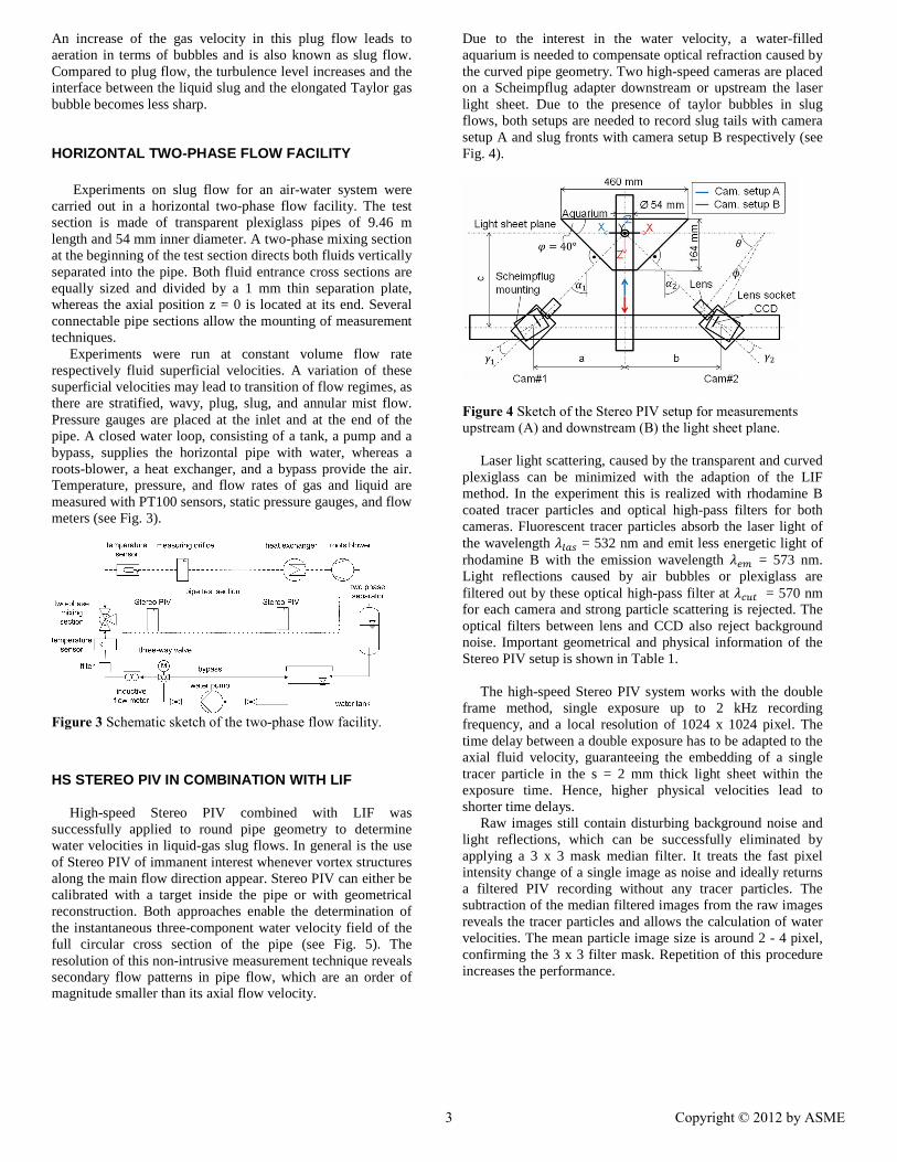
An increase of the gas velocity in this plug flow leads to aeration in terms of bubbles and is also known as slug flow. Compared to plug flow, the turbulence level increases and the interface between the liquid slug and the elongated Taylor gas bubble becomes less sharp.

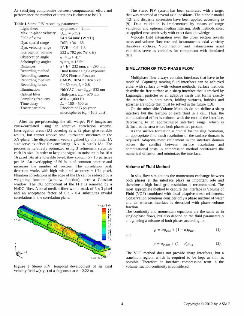
HORIZONTAL TWO-PHASE FLOW FACILITY Experiments on slug flow for an air-water system were carried out in a horizontal two-phase flow facility. The test section is made of transparent plexiglass pipes of 9.46 m length and 54 mm inner diameter. A two-phase mixing section at the beginning of the test section directs both fluids vertically separated into the pipe. Both fluid entrance cross sections are equally sized and divided by a 1 mm thin separation plate, whereas the axial position z = 0 is located at its end. Several connectable pipe sections allow the mounting of measurement techniques. Experiments were run at constant volume flow rate respectively fluid superficial velocities. A variation of these superficial velocities may lead to transition of flow regimes, as there are stratified, wavy, plug, slug, and annular mist flow. Pressure gauges are placed at the inlet and at the end of the pipe. A closed water loop, consisting of a tank, a pump and a bypass, supplies the horizontal pipe with water, whereas a roots-blower, a heat exchanger, and a bypass provide the air. Temperature, pressure, and flow rates of gas and liquid are measured with PT100 sensors, static pressure gauges, and flow meters (see Fig. 3).

Figure 3 Schematic sketch of the two-phase flow facility.

HS STEREO PIV IN COMBINATION WITH LIF High-speed Stereo PIV combined with LIF was successfully applied to round pipe geometry to determine water velocities in liquid-gas slug flows. In general is the use of Stereo PIV of immanent interest whenever vortex structures along the main flow direction appear. Stereo PIV can either be calibrated with a target inside the pipe or with geometrical reconstruction. Both approaches enable the determination of the instantaneous three-component water velocity field of the full circular cross section of the pipe (see Fig. 5). The resolution of this non-intrusive measurement technique reveals secondary flow patterns in pipe flow, which are an order of magnitude smaller than its axial flow velocity.

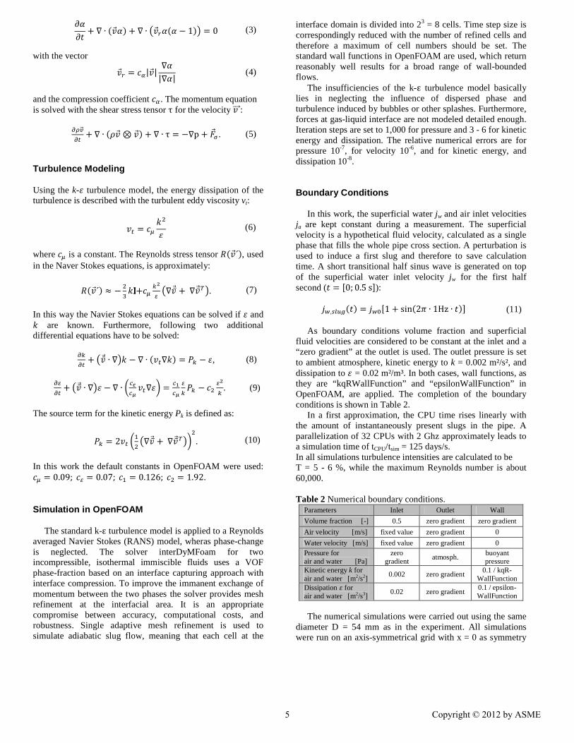
Due to the interest in the water velocity, a water-filled aquarium is needed to compensate optical refraction caused by the curved pipe geometry. Two high-speed cameras are placed on a Scheimpflug adapter downstream or upstream the laser light sheet. Due to the presence of taylor bubbles in slug flows, both setups are needed to record slug tails with camera setup A and slug fronts with camera setup B respectively (see Fig. 4).

Figure 4 Sketch of the Stereo PIV setup for measurements

upstream (A) and downstream (B) the light sheet plane. Laser light scattering, caused by the transparent and curved plexiglass can be minimized with the adaption of the LIF method. In the experiment this is realized with rhodamine B coated tracer particles and optical high-pass filters for both cameras. Fluorescent tracer particles absorb the laser light of the wavelength �� = 532 nm and emit less energetic light of rhodamine B with the emission wavelength � = 573 nm. Light reflections caused by air bubbles or plexiglass are filtered out by these optical high-pass filter at �� = 570 nm for each camera and strong particle scattering is rejected. The optical filters between lens and CCD also reject background noise. Important geometrical and physical information of the Stereo PIV setup is shown in Table 1. The high-speed Stereo PIV system works with the double frame method, single exposure up to 2 kHz recording frequency, and a local resolution of 1024 x 1024 pixel. The time delay between a double exposure has to be adapted to the axial fluid velocity, guaranteeing the embedding of a single tracer particle in the s = 2 mm thick light sheet within the exposure time. Hence, higher physical velocities lead to shorter time delays. Raw images still contain disturbing background noise and light reflections, which can be successfully eliminated by applying a 3 x 3 mask median filter. It treats the fast pixel intensity change of a single image as noise and ideally returns a filtered PIV recording without any tracer particles. The subtraction of the median filtered images from the raw images reveals the tracer particles and allows the calculation of water velocities. The mean particle image size is around 2 - 4 pixel, confirming the 3 x 3 filter mask. Repetition of this procedure increases the performance.


As satisfying compromise between computational effort and performance the number of iterations is chosen to be 10. Table 1 Stereo PIV recording parameters.

Light sheet xy-plane, s = 2 mm Max. in-plane velocity Umax = 6 m/s Field of view 54 x 54 mm² (W x H) Dyn. spatial range DSR ≈ 34 – 68 Dyn. velocity range DVR ≈ 0.9 -1.8 Interogation volume 532 x 792 pix (W x H) Observation angle α1 ≈ α2 ≈ 41°

Scheimpflug angles Distances

γ1 ≈ γ2 ≈ 12.5° a ≈ b ≈ 232 mm, c = 290 mm

Recording method Dual frame / single exposure Recording camera Recording medium

APX Photron Fastcam CMOS, 1024 x 1024 pixel

Recording lenses f = 60 mm, f# = 2.8 Illumination Nd:YAG laser ��= 532 nm Optical filter High-pass: λcut = 570 nm Sampling frequeny Time delay

450 – 1,000 Hz ∆t = 150 – 500 µs

Tracer particles Rhodamine B polymer microspheres (dp ≈ 10.5 µm)

After the pre-processing, the still warped PIV images are cross-correlated using an adaptive correlation scheme. Interrogation areas (IA) covering 32 x 32 pixel give reliable results, but cannot resolve small turbulent structures in the XY-plane. The displacement vectors gained by this initial IA size serve as offset for correlating 16 x 16 pixels IAs. The process is iteratively optimized using 3 refinement steps for each IA size. In order to keep the signal-to-noise ratio for 16 x 16 pixel IAs at a tolerable level, they contain 5 - 10 particles per IA. An overlapping of 50 % is of common practice and increases the number of vectors. The correlation peak detection works with high sub-pixel accuracy ~ 1/64 pixel. Phantom correlations at the edge of the IA can be reduced by a weighting function (window function), here a Gaussian window. The DC component of the FFT is removed by a NoDC filter. A local median filter with a mask of 3 x 3 pixel and an acceptance factor of 0.3 - 0.4 substitutes invalid correlations in the correlation plane.

Figure 5 Stereo PIV: temporal development of an axial velocity field w(x,y,t) of a slug onset at z = 2.22 m.

The Stereo PIV system has been calibrated with a target that was recorded at several axial positions. The pinhole model [12] and disparity correction have been applied according to [9]. Data validation is implemented by means of range validation and optional median filtering. Both methods must be applied case sensitively with exact data knowledge. Velocity field integration over the cross section reveals mass and volume flow rate and instantaneous axial vorticity dissolves vortices. Void fraction and instanateaous axial velocities serve as variables for comparison with simulated data. SIMULATION OF TWO-PHASE FLOW Multiphase flow always contains interfaces that have to be modeled. Capturing moving fluid interfaces can be achieved either with surface or with volume methods. Surface methods describe the free surface as a sharp interface that is tracked by Lagrangian particles or an adaptive mesh that forms exactly the interface. In both cases, folding surfaces, bubbles and splashes are topics that must be solved in the future [13]. On the other side Volume Methods do not define a sharp interface but the fraction of each fluid in a cell. Thus, the computational effort is reduced with the cost of the interface, decreasing to an approximated interface range, which is defined as the area where both phases are present. As the surface formation is crucial for the slug formation, an appropriate fine mesh resolution of the surface domain is required. Adaptive mesh refinement in the interface domain solves the conflict between surface resolution and computational costs. A compression method counteracts the numerical diffusion and minimizes the interface. Volume of Fluid Method In slug flow simulations the momentum exchange between both phases at the interface plays an important role and therefore a high local grid resolution is recommended. The most appropriate method to capture the interface is Volume of Fluid (VOF) combined with local adaptive mesh refinement. Conservation equations consider only a phase mixture of water and air whereas interface is described with phase volume fraction. The continuity and momentum equations are the same as in single-phase flows, but also depend on the fluid parameters � and� being a mixture of both phases according to: � � �� 1 � �� (1) and � � �� 1 � ��. (2) The VOF method does not provide sharp interfaces, but a transition region, which is required to be kept as thin as possible. Therefore an interface compression term in the volume fraction continuity is considered:


��

� ∇ ∙ �� ∇ ∙ ��!�� 1�" = 0 (3)

with the vector ��! = $%|��| ∇�

|∇�| (4)

and the compression coefficient $%. The momentum equation is solved with the shear stress tensor τ for the velocity �(((�:

)*+(�

) + ∇ ∙ �� ⊗ �� + ∇ ∙ τ = −∇p + .�/. (5)

Turbulence Modeling Using the k-� turbulence model, the energy dissipation of the turbulence is described with the turbulent eddy viscosity vt:

� = $0 12

� (6)

where $0 is a constant. The Reynolds stress tensor 3��´�, used in the Naver Stokes equations, is approximately: 3��´� ≈ − 2

6 1IIII+$0 89: ∇�̅� +∇�̅�<". (7)

In this way the Navier Stokes equations can be solved if � and 1 are known. Furthermore, following two additional differential equations have to be solved: )8

) + �̅� ∙ ∇"1 − ∇ ∙ �� ∇1� = =8 − �, (8)

):

) + �̅� ∙ ∇"� − ∇ ∙ >�?�@ � ∇�A = �B

�@:8 =8 − $2 :9

8 . (9)

The source term for the kinetic energy Pk is defined as: =8 = 2� >D2 ∇�̅� + ∇�̅�<"A

2. (10)

In this work the default constants in OpenFOAM were used: $0 = 0.09;$: = 0.07;$D = 0.126;$2 = 1.92. Simulation in OpenFOAM The standard k-ε turbulence model is applied to a Reynolds averaged Navier Stokes (RANS) model, wheras phase-change is neglected. The solver interDyMFoam for two incompressible, isothermal immiscible fluids uses a VOF phase-fraction based on an interface capturing approach with interface compression. To improve the immanent exchange of momentum between the two phases the solver provides mesh refinement at the interfacial area. It is an appropriate compromise between accuracy, computational costs, and robustness. Single adaptive mesh refinement is used to simulate adiabatic slug flow, meaning that each cell at the

interface domain is divided into 23 = 8 cells. Time step size is correspondingly reduced with the number of refined cells and therefore a maximum of cell numbers should be set. The standard wall functions in OpenFOAM are used, which return reasonably well results for a broad range of wall-bounded flows. The insufficiencies of the k-ε turbulence model basically lies in neglecting the influence of dispersed phase and turbulence induced by bubbles or other splashes. Furthermore, forces at gas-liquid interface are not modeled detailed enough. Iteration steps are set to 1,000 for pressure and 3 - 6 for kinetic energy and dissipation. The relative numerical errors are for pressure 10-7, for velocity 10-6, and for kinetic energy, and dissipation 10-8. Boundary Conditions In this work, the superficial water jw and air inlet velocities ja are kept constant during a measurement. The superficial velocity is a hypothetical fluid velocity, calculated as a single phase that fills the whole pipe cross section. A perturbation is used to induce a first slug and therefore to save calculation time. A short transitional half sinus wave is generated on top of the superficial water inlet velocity jw for the first half second (� = K0; 0.5sN):

OP,�� = OPRK1 + sin�2U ∙ 1Hz ∙ ��N (11)

As boundary conditions volume fraction and superficial fluid velocities are considered to be constant at the inlet and a “zero gradient” at the outlet is used. The outlet pressure is set to ambient atmosphere, kinetic energy to k = 0.002 m²/s², and dissipation to � = 0.02 m²/m³. In both cases, wall functions, as they are “kqRWallFunction” and “epsilonWallFunction” in OpenFOAM, are applied. The completion of the boundary conditions is shown in Table 2. In a first approximation, the CPU time rises linearly with the amount of instantaneously present slugs in the pipe. A parallelization of 32 CPUs with 2 Ghz approximately leads to a simulation time of tCPU/tsim = 125 days/s. In all simulations turbulence intensities are calculated to be T = 5 - 6 %, while the maximum Reynolds number is about 60,000. Table 2 Numerical boundary conditions.

Parameters Inlet Outlet Wall

Volume fraction [-] 0.5 zero gradient zero gradient

Air velocity [m/s] fixed value zero gradient 0

Water velocity [m/s] fixed value zero gradient 0 Pressure for air and water [Pa]

zero gradient

atmosph. buoyant pressure

Kinetic energy k for air and water [m2/s2]

0.002 zero gradient 0.1 / kqR-

WallFunction Dissipation � for air and water [m2/s3]

0.02 zero gradient 0.1 / epsilon- WallFunction

The numerical simulations were carried out using the same diameter D = 54 mm as in the experiment. All simulations were run on an axis-symmetrical grid with x = 0 as symmetry


plane. The cross section is generated out of six domains, two quadratic in the center and four O-meshes in the surrounding area (see Fig. 6). All presented numerical cases start with an adequate amount of 294 cells per cross section.

Figure 6 Pipe geometry: main block meshes (left) and grid resolution with single mesh refinement at a random time step (right). The axial length as well as the corresponding number of cells depend on the test cases and are depicted in Table 3. Using mesh refinement, the initial mesh size will increase with the interface shape complexity and consequently with time. Table 3 Parameters of simulation cases.

Cas

e Type of

flow

Pipe Lengt

h [ m ]

Axial cell number [-]

Mesh refinement

Superfic. inlet velocity [m/s]

water air

A slug 4.00 200 no 1.00* 0.5 B slug 4.00 400 no 1.00* 0.5 C slug 4.00 400 yes 1.00* 0.5 D pipe 1.62 162 no 0.69 - E pipe 1.62 162 no 1.06 -

F slug onset

10.00 1,000 yes 0.70* 0.56

G slug exp.

10.00 1,000 yes 0.70* 0.56

*Transitional pertubation Grid Independence Study A test case for a L = 4 m long pipe was run (L/D = 74.1) with three different axial mesh resolutions to determine the influence of the mesh-resolution on predicted results: A) axial lowly resolved static mesh (200 cells), B) axial highly resolved static mesh (400 cells), and C) axial highly resolved mesh with single step adaptive mesh refinement (400 cells). All three cases start with a transitional water velocity at the inlet, respectively a temporary velocity perturbation. In cases A and B a first slug is induced, whereas in case C, due to the adaptive-mesh, slugs are continuously initiated. Figure 7 shows an instantaneous axial void-fraction distribution at the time-step t = 6.94 s. It illustrates that case A produces stratified flow, case B wavy flow whereas case C shows the ability to reproduce slug flow. This becomes clear in Figure 8, where the inlet pressure at z = 0 is depicted as a function of time. Pressure peaks reveal the presence of slugs in the pipe and furthermore an approximately constant slug frequency.

Static meshes with moderate mesh resolution as in A and B do not resolve the interface properly and hence are not capable of generating self-induced slugs as in case C. A higher resolution does not eminently improve the reproduction of slugs whereas lower resolution changes the results to non-physical behavior. Due to mesh refinement and a certain Courant number, calculation time especially rises with the number of present slugs in the pipe. This implies that the calculation time step size is correspondingly reduced if the mesh is refined.

Figure 7 Instantaneous void fraction of the mesh test cases A, B, and C across the pipe at the time step t = 6.94 s.

Figure 8 Inlet pressure of the mesh test cases A, B, and C as function of time.

Comparison of URANS and Stereo PIV with Regards to Pipe Flow

A comparison of axial velocity between experimental and numerical pipe flow was done for two water superficial velocities. It acts in first approximation as an indicator for the quality of results. Two pipe flow cases D and E with inlet water velocities of jliq = 0.69 m/s and jliq = 1.06 m/s respectively are evaluated in the experiment and simulation (see Tab. 4). The vertical profile of the mean axial velocity w (y, x = 0) is calculated in the experiment out of 200 vector fields, recorded with the frequency frec = 400 Hz at the axial position z = 2.22 m. Due to the steadiness of pipe flow in the numerical simulation, it is sufficient to analyze the flow within a short pipe of 1.62 length at the axial position z = 0.80 m. This leads to a ratio of z/D = 14.8 in the simulation and 41 in the experiment, where fully developed flow is ensured. Due to


single-phase flow, no mesh refinement takes place. The mean axial velocity is determined by the integration over the cross section. Table 4 Water inlet velocities for pipe flow.

Pipe flow Case D Case E

Exp. Num. Exp. Num. Superfic. water inlet vel. [m/s] 0.69 0.69 1.06 1.06 Mean axial water vel. w [m/s] 0.64 0.69 0.99 1.06

Standard deviation of w [mm/s] 1.2 - 2.3 -

Analysis plane at ax.length z[m] (Total pipe length L) [m]

2.22 (9.64)

0.80 (1.62)

2.22 (9.64)

0.80 (1.62)

Due to the conservation of mass continuity, the axial mean flow in the simulation is the same as at the inlet position. Experiments give a relative error of the mean axial water velocity for case D of � = 7.8 % and for case E of � = 7.1 %. Furthermore, the time-averaged axial velocity profile w(y) serves as quality indicator for the results and also as comparability of the simulation with the experiment. Figure 9 shows good agreement in both cases, whereas simulations reveal smoother profiles due to the k-� turbulence model than the experiments.

Figure 9 Vertical profiles of time-averaged axial velocities for pipe flow D and E for Stereo PIV and URANS. On the one hand this is caused by flow turbulence, which URANS does not resolve sufficiently; on the other hand the short recording time in the experiment reveals velocity. Comparison of URANS and Stereo PIV with regards to the Onset of a Slug

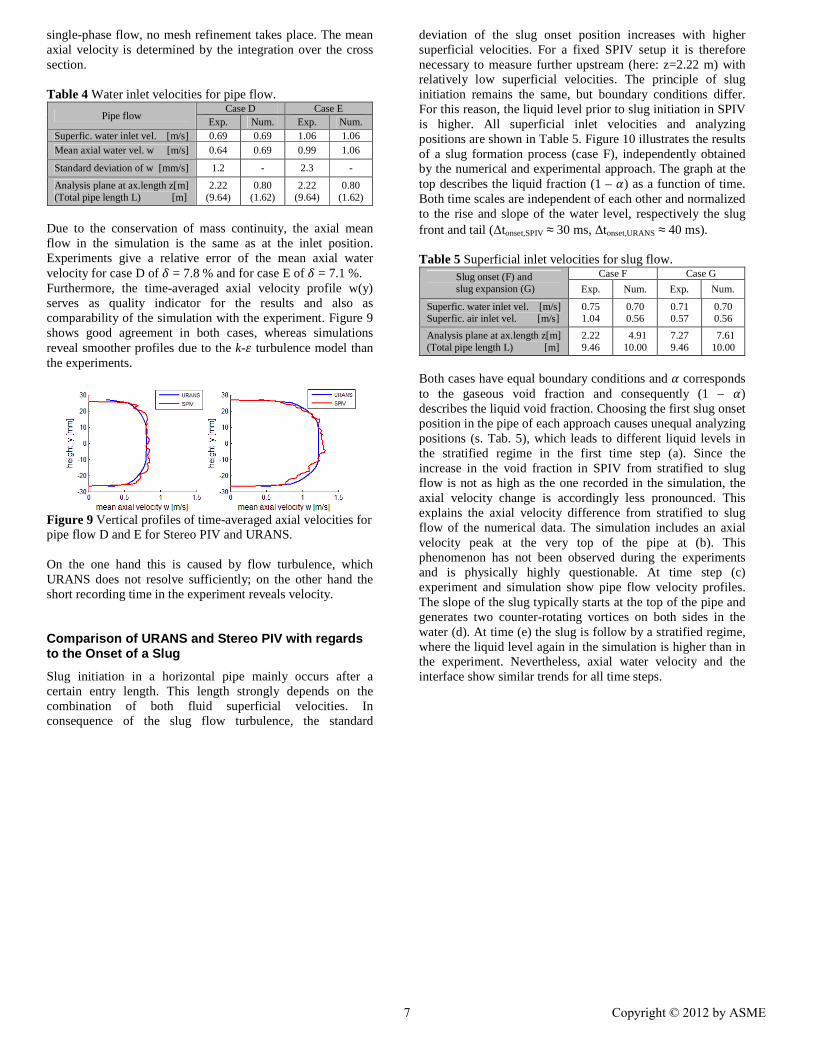
Slug initiation in a horizontal pipe mainly occurs after a certain entry length. This length strongly depends on the combination of both fluid superficial velocities. In consequence of the slug flow turbulence, the standard

deviation of the slug onset position increases with higher superficial velocities. For a fixed SPIV setup it is therefore necessary to measure further upstream (here: z=2.22 m) with relatively low superficial velocities. The principle of slug initiation remains the same, but boundary conditions differ. For this reason, the liquid level prior to slug initiation in SPIV is higher. All superficial inlet velocities and analyzing positions are shown in Table 5. Figure 10 illustrates the results of a slug formation process (case F), independently obtained by the numerical and experimental approach. The graph at the top describes the liquid fraction (1 – �) as a function of time. Both time scales are independent of each other and normalized to the rise and slope of the water level, respectively the slug front and tail (∆tonset,SPIV ≈ 30 ms, ∆tonset,URANS ≈ 40 ms). Table 5 Superficial inlet velocities for slug flow.

Slug onset (F) and slug expansion (G)

Case F Case G

Exp. Num. Exp. Num.

Superfic. water inlet vel. [m/s] Superfic. air inlet vel. [m/s]

0.75 1.04

0.70 0.56

0.71 0.57

0.70 0.56

Analysis plane at ax.length z[m] (Total pipe length L) [m]

2.22 9.46

4.91 10.00

7.27 9.46

7.61 10.00

Both cases have equal boundary conditions and � corresponds to the gaseous void fraction and consequently (1 – �) describes the liquid void fraction. Choosing the first slug onset position in the pipe of each approach causes unequal analyzing positions (s. Tab. 5), which leads to different liquid levels in the stratified regime in the first time step (a). Since the increase in the void fraction in SPIV from stratified to slug flow is not as high as the one recorded in the simulation, the axial velocity change is accordingly less pronounced. This explains the axial velocity difference from stratified to slug flow of the numerical data. The simulation includes an axial velocity peak at the very top of the pipe at (b). This phenomenon has not been observed during the experiments and is physically highly questionable. At time step (c) experiment and simulation show pipe flow velocity profiles. The slope of the slug typically starts at the top of the pipe and generates two counter-rotating vortices on both sides in the water (d). At time (e) the slug is follow by a stratified regime, where the liquid level again in the simulation is higher than in the experiment. Nevertheless, axial water velocity and the interface show similar trends for all time steps.


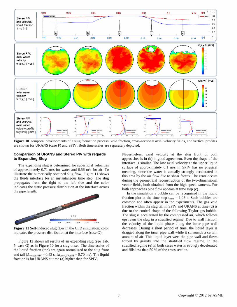
Figure 10 Temporal developments of a slug formation process: void fraction, cross-sectional axial velocity fields, and vertical profiles are shown for URANS (case F) and SPIV. Both time scales are separately depicted.

Comparison of URANS and Stereo PIV with regards to Expanding Slug

The expanding slug is determined for superficial velocities of approximately 0.71 m/s for water and 0.56 m/s for air. To illustrate the numerically obtained slug flow, Figure 11 shows the fluids interface for an instantaneous time step. The slug propagates from the right to the left side and the color indicates the static pressure distribution at the interface across the pipe length.

Figure 11 Self-induced slug flow in the CFD simulation: color indicates the pressure distribution at the interface (case G). Figure 12 shows all results of an expanding slug (see Tab. 5, case G) as in Figure 10 for a slug onset. The time scales of the liquid fraction (top) are again normalized to the slug front and tail (∆tonset,SPIV ≈ 0.43 s, ∆tonset,URANS ≈ 0.70 ms). The liquid fraction is for URANS at time (a) higher than for SPIV.

Nevertheless, axial velocity at the slug front of both approaches is in (b) in good agreement. Even the shape of the interface is similar. The low axial velocity at the upper liquid surface of approximately 0.1 m/s in SPIV has no physical meaning, since the water is actually strongly accelerated in this area by the air flow due to shear forces. The error occurs during the geometrical reconstruction of the two-dimensional vector fields, both obtained from the high-speed cameras. For both approaches pipe flow appears at time step (c). In the simulation a bubble can be recognized in the liquid fraction plot at the time step tnum = 1.05 s. Such bubbles are common and often appear in the experiments. The gas void fraction within the slug tail in SPIV and URANS at time (d) is due to the conical shape of the following Taylor gas bubble. The slug is accelerated by the compressed air, which follows upstream the slug in a stratified regime. Due to wall friction, the velocity of the liquid phase along the inner pipe wall decreases. During a short period of time, the liquid layer is dragged along the inner pipe wall while it surrounds a certain amount of air. This liquid layer wets the pipe wall and flows forced by gravity into the stratified flow regime. In the stratified regime (e) in both cases water is strongly decelerated and fills less than 50 % of the cross section.


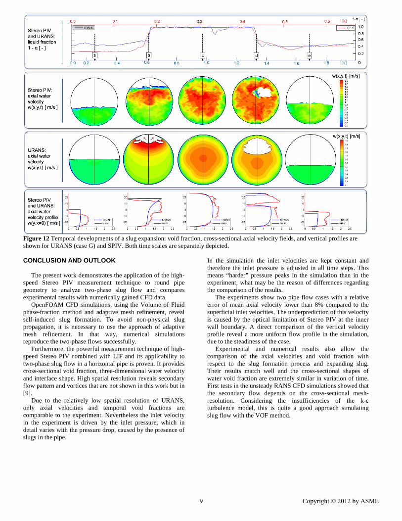
Figure 12 Temporal developments of a slug expansion: void fraction, cross-sectional axial velocity fields, and vertical profiles are shown for URANS (case G) and SPIV. Both time scales are separately depicted. CONCLUSION AND OUTLOOK The present work demonstrates the application of the high-speed Stereo PIV measurement technique to round pipe geometry to analyze two-phase slug flow and compares experimental results with numerically gained CFD data. OpenFOAM CFD simulations, using the Volume of Fluid phase-fraction method and adaptive mesh refinement, reveal self-induced slug formation. To avoid non-physical slug propagation, it is necessary to use the approach of adaptive mesh refinement. In that way, numerical simulations reproduce the two-phase flows successfully. Furthermore, the powerful measurement technique of high-speed Stereo PIV combined with LIF and its applicability to two-phase slug flow in a horizontal pipe is proven. It provides cross-sectional void fraction, three-dimensional water velocity and interface shape. High spatial resolution reveals secondary flow pattern and vortices that are not shown in this work but in [9]. Due to the relatively low spatial resolution of URANS, only axial velocities and temporal void fractions are comparable to the experiment. Nevertheless the inlet velocity in the experiment is driven by the inlet pressure, which in detail varies with the pressure drop, caused by the presence of slugs in the pipe.

In the simulation the inlet velocities are kept constant and therefore the inlet pressure is adjusted in all time steps. This means “harder” pressure peaks in the simulation than in the experiment, what may be the reason of differences regarding the comparison of the results. The experiments show two pipe flow cases with a relative error of mean axial velocity lower than 8% compared to the superficial inlet velocities. The underprediction of this velocity is caused by the optical limitation of Stereo PIV at the inner wall boundary. A direct comparison of the vertical velocity profile reveal a more uniform flow profile in the simulation, due to the steadiness of the case. Experimental and numerical results also allow the comparison of the axial velocities and void fraction with respect to the slug formation process and expanding slug. Their results match well and the cross-sectional shapes of water void fraction are extremely similar in variation of time. First tests in the unsteady RANS CFD simulations showed that the secondary flow depends on the cross-sectional mesh-resolution. Considering the insufficiencies of the k-ε turbulence model, this is quite a good approach simulating slug flow with the VOF method.


Large Eddy Simulation (LES) would improve spatial resolution, but it is not appropriate to use due to the enormous amount of cells in the large pipe volume. To simulate smaller vortex structures for this highly unsteady two-phase slug phenomenon, there is the possibility to start simulations with URANS and to switch at a certain time step prior to a slug formation to LES. So far, these CFD calculations give very promising results but used computational effort does not allow complete evaluations. The authors are grateful for the financial support of the German Federal Ministry of Economics and Technology (BMWi) that founded the research project under the project number 1501359. Responsibility for the content of this paper lies with the author. REFERENCES

[1] Jansen F. E., Shoham O., and Taitel Y., 1996, “The Elimination of Severe Slugging - Experiments and Modeling,” Int. J. Multiphase Flow, Vol.22, No, pp. 1055-1072.

[2] Fernandez-Betancor G., Hale C. P., Hewitt G. F., Morgan R. G., and Ujang P., 2007, “Slug initiation and development in horizontal two-phase flow,” Chemical Engineering, pp. 1-13.

[3] Chen J., and Spedding P. L., 1983, “An analysis of holdup in horizontal two-phase gas-liquid flow,” International Journal of Multiphase Flow, 9(2), pp. 147-159.

[4] Höhne T., and Vallée C., 2010, “Experiments and numerical Simulations of horizontal Two-Phase Flow Regimes Using an Interfacial Area Density Model,” Journal of Computational Multiphase Flows, Volume 2, pp. 131-143.

[5] Prasser H.-M., Scholz D., and Zippe C., 2001, “Bubble size measurement using wire-mesh sensors,” Flow Measurement and Instrumentation, 12, pp. 299-312.

[6] Kallweit S., Kaminsky R., and van Canneyt Coon E. S., 2007, “Hispeed und Stereo PIV in einem künstlichen Blutgefäß,” Fachtagung “Lasermethoden in der Strömungsmesstechnik,” 48, pp. 1-4.

[7] van Doornel C. W. H., Hof B., Lindken R. H., Westerweel J., and Dierksheide U., 2003, “Time Resolved Stereoscopic PIV in Pipe Flow. Visualizing 3D Flow Structures,” 5th International Symposium on Particle Image Velocimetry, Paper 3132, pp. 1-11.

[8] Lindken R., and Merzkirch W., 2002, “A novel PIV technique for measurements in multiphase flows and its application to two-phase bubbly flows,” Experiments in Fluids, 33, pp. 814-825.

[9] Czapp M., Utschick M., and Sattelmayer T., 2011, “Stereo PIV Investigations on Slug Flows in a Horizontal Pipe,” Fachtagung “Lasermethoden in der Stroemungsmesstechnik.”

[10] Frank T., 2005, “Numerical Simulation of Slug Flow Regime for an Air-Water Two-Phase Flow in Horizontal Pipes,” NURETH-11, paper: 038, pp. 1-13.

[11] Vallee C., Hoehne T., Prasser H.-M., and Suehnel T., 2007, Experimental investigation and CFD simulation of slug flow in horizontal channels.

[12] Raffel M., Willert C. E., Wereley S. T., and Kompenhans J., 2007, Particle Image Velocimetry, Springer-Verlag Berlin Heidelberg New York.

[13] Marschall H., and Hinrichsen O., “Numerical Simulation of Multiscale Two-Phase Flows using a Hybrid Interface-Resolving Two-Fluid Model (HIRES-TFM),” p. 1.


Documents

Investigations on Slug Flow in a Horizontal Pipe Using