QUASI-3D MODELLING OF TWO-PHASE SLUG FLOW IN · PDF filethe slug flow regime in horizontal pipes is presented in the paper by Frank (2005). In general, the current two major modeling

Ninth International Conference on CFD in the Minerals and Process Industries

CSIRO, Melbourne, Australia

10-12 December 2012

Copyright © 2012 CSIRO Australia 1

QUASI-3D MODELLING OF TWO-PHASE SLUG FLOW IN PIPES

Sjur MO*1)

, Alireza ASHRAFIAN1)

, Jean-Christophe BARBIER2)

& Stein Tore JOHANSEN1)

1)Flow Technology Group, SINTEF Materials and Chemistry, 7465 Trondheim, NORWAY

2)Total E&P, Norway, Stavanger

*Corresponding author’s e-mail: [email protected]

ABSTRACT

In this paper, we present progress obtained by the Quasi 3-

Dimensional (Q3D) model for pipe flows. This model is

based on a multi-fluid multi-field formulation with

construction and tracking of the large-scale interfaces

(LSIs). Here the computational time is significantly

reduced by performing a slice-averaging technique.

However, new terms are created in the model equations

which are related to the important mechanisms such as

wall shear stress and turbulence production at side walls.

The paper reports some basic performance of the model,

including single phase wall friction and the velocities of

single Taylor bubbles at inclinations ranging from

horizontal to vertical. Finally we report the performance of

the model for slug flow in horizontal and 10° inclined

pipes.

The model seems to satisfactorily reproduce the two

investigated slug flows. This indicates that the model can

have a great potential is serving the oil & gas industry.

NOMENCLATURE

D Pipe diameter (m)

Fr Froude number ( driftFr v gD� )

driftv Drift velocity (m/s)

g Gravity (9.81 m/s2)

mk Turbulent kinetic energy for phase m (m2/s2)

l Turbulent length scale (m)

DRe Pipe Reynolds number ( DRe UD� �� )

U Stream wise velocity (m/s)

� Wall roughness (m)

m� Turbulent dissipation for phase m (m2/s3)

m� Molecular viscosity for phase m (Pa�s)

T

m� Turbulent viscosity for phase m (Pa�s)

m� Density for phase m (kg/m3)

INTRODUCTION

In industrial pipelines for oil and gas transport unstable

flows can cause major operational problems. A main

problem is that the liquid is arriving in larger, intermittent

chunks (slugs), and not continuously. In this case a

separator with huge volume would be needed to handle

the liquid in such large slugs. These instabilities are

caused by liquid waves that grow and interact to form

hydrodynamic slugs. Empirically it has been observed that

these hydrodynamic slugs can grow continuously with

time and form huge slugs (Shea et al., 2004). However, the

mechanisms of initial slug formation are poorly

understood, together with the growth mechanisms which

lead to the manifestation of large and industrially

problematic slugs.

SINTEF, ConocoPhillips and Total have been working

with development of the LedaFlow multiphase flow

prediction tools (Laux et al., 2007, 2008a, 2008b) to

enable more fundamental prediction of multiphase flows,

including the phenomena of slugging. The overall idea has

been to develop a model which is capable of handling

most multiphase flow phenomena that will appear in a

pipeline. Typical situations to predict are two and three

phase flows where the flow patterns include waves and

distribution of dispersed fields. The flow pattern should be

fundamentally predicted by the model. In addition, the

model should be sufficiently fast to analyze the flow in a

relevant pipeline length. The results presented in this

paper show the capabilities of this model for some

selected applications.

Modeling of slug flow in pipes

The main mechanism leading to the formation of the

liquid slugs in pipes and channels is the retardation of the

liquid phase by wall friction. Due to incompressibility and

conservation of the volume of the liquid phase, the liquid

level is slightly rising with increasing distance along the

pipe. Simultaneously, this leads to acceleration of the gas

phase in the upper part of the pipe leading to increasing

local gas velocities and corresponding pressure drop. If a

critical velocity difference between the two phases is

exceeded, the interface become unstable and wavy

structures develop. Further reduction in the local gas

pressure reinforces the build-up of the wave which leads

to complete blockage of the pipe-cross section by the

liquid phase and hence formation of a liquid slug. The

blockage of the cross-sectional area gives rise to a steep

pressure-gradient in the gas phase which drives the liquid

slug. Depending on the pipe geometry (length and

diameter) and the gas and liquid flow rates, the slug flow

regime can be stable, in which liquid slugs move over long

distances in the pipe, or, in other cases, liquid slugs

disintegrate after a certain distance of propagation due to

loss of the critical liquid mass contained in the slug.

Successful modeling of hydrodynamic slug flow poses

several challenges. One of them is modeling the dynamic

behavior of the interface which separates the two layers of

fluid but, at the same time, where significant entrainment

and mixing takes place, leading to simultaneous dispersion


of gas bubbles into the liquid and liquid droplets into the

gas. These phenomena, as well as the prediction of the

bubble and droplet size, have significant importance in

determining the slug flow regime and are very difficult to

predict due to the complex turbulence phenomena taking

place at and in the vicinity of the large scale interface. Due

to these effects, accurate physical predictions are beyond

the current 1D-modeling capabilities. Hence, we need to

address the slug flow process by applying more

fundamental principles.

A review on past attempts towards numerical simulation of

the slug flow regime in horizontal pipes is presented in the

paper by Frank (2005). In general, the current two major

modeling approaches for modeling of dispersed and

separated flows, the standard multi-fluid Eulerian and the

volume-of-fluid (VOF) methods, are not fully capable of

handling situations where large scale interfaces and

dispersion of phases co-exist. Multi-fluid models are well

suited for dispersed flows (with no large scale interfaces)

whereas the VOF models are well-suited for separated

flows with no mixing at the interface.

The three dimensional nature of the slug flow in pipes has

a crucial significance that cannot be ignored. Firstly, and

as discussed earlier, formation of the slug flow is strongly

influenced and determined by the wall friction on the

liquid phase. In a plane 2D approximation of the slug flow

in pipe, the effect of sidewalls on the flow is neglected and

therefore, the extra retardation of the liquid phase by the

pipe walls is less emphasized compared to a full 3D flow.

Secondly, the total blockage of the cross sectional area by

the liquid phase is more easily established in pipes than in

channels. Therefore, plane 2D modeling of slug flow in

pipes cannot yield good predictions.

Full 3D simulations of slug flow in pipes are very

expensive in terms of computational time, memory

requirements, data storage and post-processing. Compared

to the diameter of the pipe, the length of the pipe has to be

sufficiently long so that hydrodynamic slugs can be

generated (see e.g. Lakehal et al. 2012). Hence, a 3D

based method, averaged down to two dimensions, may

offer a good compromise of speed and accuracy. This

approach is explained next.

MODEL DESCRIPTION

Model basis

The model is based on a 3D and 3-phase formulation,

where the equations are derived based on volume

averaging and ensemble averaging of the Navier-Stokes

equations. Conceptually, the model is based on the

following elements (Laux et al., 2007):

i) A multi-fluid Eulerian model allowing two types of

dispersed fields in each of the three continuous fluids.

ii) The flow domain consists of several zones, each with

a well-defined continuous fluid, separated by LSIs

iii) Between the zones local boundary conditions are

applied (interface fluxes)

iv) Field based turbulence model with wall functions for

interfaces and solid walls.

v) Evolution models for droplet and bubble sizes

vi) By adding together the field-based equations phase

based mass, momentum and turbulence equations are

obtained

For the turbulence model we have here applied a length

scale model, which is solved from a Poisson equation. At

solid walls and LSIs the length scale is given as a

boundary condition. Turbulent energy equations are

solved for each phase, again applying wall laws at solid

walls and the LSIs. The turbulent viscosity for phase m

is given by:

0.35T

m m ml k� �� (1)

The turbulent dissipation rate for phase m is:

1.50.35 /

m mk l� � (2)

The resulting model gives the volume fractions and

momentum for the phases in the flow. In order to apply

local boundary conditions inside the flow as described

above we need to identify the Large Scale interfaces. This

is done based on an evaluation of the predicted phase

volume fraction, based on the assumption that there is a

critical volume fraction which controls phase inversion. In

this work a phase is continuous if the local volume

fraction is above 0.5. Based on a relative simple

reconstruction algorithm, the interface is reconstructed

such that the local boundary conditions can be applied.

Presently, the effects of surface tension on the motion of

the Large Scale Interface are not included. This

simplification is good as long as we use relatively coarse

grids and do not want to resolve capillary waves.

This model framework has the capability to handle any 3D

3-phase (or less) multiphase flow as long as the flow can

be described by 9 fields – 3 continuous fields with 2

dispersed fields in each. However, fields such as thin

liquid wall films are not included. As this model is

directed towards predictions of multiphase flows in

pipelines long sections of pipes will have to be simulated

for a considerable flow-time. This restriction demands

simplifications in order to be able to obtain results in a

reasonable time. Weeks or months of computer time on

parallel machines would not be acceptable for most

industrial applications. The simplification we have

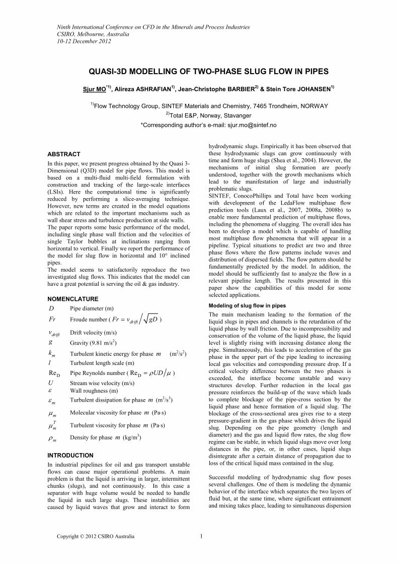
introduced is the Quasi 3D (Q3D) approximation. By

slicing the pipe in one direction (usually the vertical

direction), as demonstrated in Figure 1, the flow can be

resolved as 2-dimensional, but describing the complete

flow in a pipe.

Figure 1: Quasi 3D grid cells, showing one axial (x-

direction) and 7 vertical cells.

The full 3D model equations are then averaged over the

transversal distance z to create slice averaged model

equations. In this process the 3D structures are

homogenized and the flow becomes represented by slice

averaged fields. One result is that the wall fluxes, such as

shear stresses, becomes source terms in what we call


Quasi-3D (Q3D) model equations (for details, see Laux et

al., 2007).

The numerical solution is performed on a staggered

Cartesian mesh, where the discrete mass, pressure and

momentum equations are solved by an extended phase-

coupled SIMPLE method (Patankar, 1980). The implicit

solver uses first order-time discretization and up to third-

order in space (convective terms, Laux et al., 2007).

The Quasi 3D model description is expected to perform

well in horizontal stratified and hydrodynamic slug flows

where the large scale interface is dominantly horizontal at

a given axial position x , as seen in Figure 11 and

demonstrated in previous papers (Laux et al., 2007, 2008a,

2008b).

The applicability of the Q3D approximation to high

inclination and vertical flows can only be clarified by

testing the model versus experiments. This will be

discussed below.

BASIC MODEL PERFORMANCE

Performance tests

In order to verify the model single phase calculations were

performed to check the prediction quality of wall shear

stresses and the resulting pressure drop. In the verification

runs good agreement with slice averaged profiles of

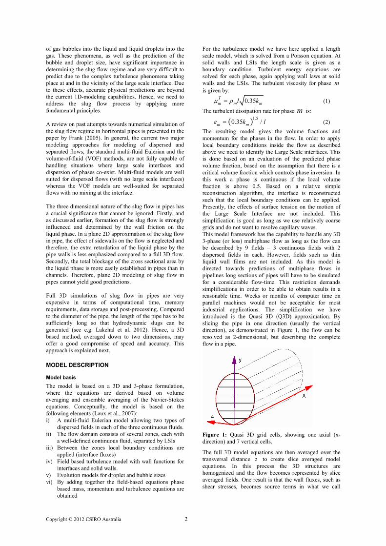
velocity and turbulent energy was obtained. In Figure 2 we

see that the model gives acceptable single phase pressure

drops over the entire range of Reynolds numbers and wall

roughnesses ε.

Figure 2: Moody diagram (Moody 1944) showing friction

factor calculated using the Colebrook (1939) equation

(lines) and Q3D (squares) for different relative wall

roughnesses ε /D versus pipe Reynolds number.

As a symmetry test the model was tested for the Rayleigh–

Taylor instabilities for all spatial directions. It has also

been demonstrated that it is possible to obtain the Kelvin

Helmholtz instability.

Further validation of the model is discussed next.

Taylor bubble velocities

Another fundamental check of the model is its capability

to reproduce the velocity of Taylor bubbles in two phase

flows. Accurate representation of the speed of Taylor

bubbles, in both horizontal and inclined pipes, is essential

for modeling slugs under operational conditions. We

therefore investigate the Q3D model's capability to handle

Taylor bubbles in pipes with various inclinations, ranging

from horizontal to vertical. In a recent paper Jeyachandra

et al. (2012) reported measurements of drift velocity for

air bubbles in high viscosity oils for different inclinations

and pipe diameters. The oil viscosities were

(0.105,0.256,0.378,0.574) Pa�s, the inclinations (0°,10°,

30°,50°,70°,90°) and the pipe diameters (2,3,6) inches. In

Figure 5 we compare the results for diameter 76.2 mm and

oil viscosity 574 mPa�s with CFD results both from Fluent

3D and Q3D. The pipe length was 4 m. For the Q3D

simulations we used a 600�15 mesh1 while the Fluent

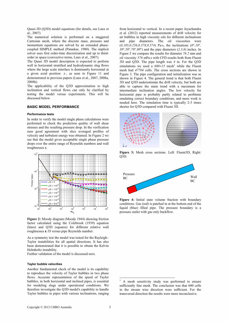
mesh had 47704 cells. The cross sections are shown in

Figure 3. The pipe configuration and initialization was as

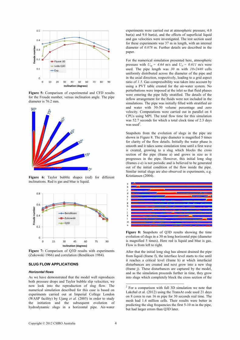
shown in Figure 4. The general trend is that both Fluent

3D and Q3D underestimate the drift velocity, but both are

able to capture the main trend with a maximum for

intermediate inclination angles. The low velocity for

horizontal pipe is probably partly related to problems

emulating correct boundary conditions, and more work is

needed here. The simulation time is typically 2-3 times

shorter for Q3D compared with Fluent 3D.

Figure 3: Mesh cross sections. Left: Fluent3D, Right:

Q3D.

Figure 4: Initial state volume fraction with boundary

conditions. Gas (red) is patched in at the bottom end of the

liquid (blue) filled pipe. The pressure boundary is a

pressure outlet with gas only backflow.

1 A mesh sensitivity study was performed to ensure

sufficiently fine mesh. The conclusion was that 600 cells

in the stream wise direction were sufficient. For the

transversal direction the results were more inconclusive.

Wall

BC

Pressure

BC


Figure 5: Comparison of experimental and CFD results

for the Froude number, versus inclination angle. The pipe

diameter is 76.2 mm.

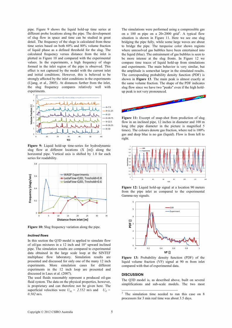
Figure 6: Taylor bubble shapes (red) for different

inclinations. Red is gas and blue is liquid.

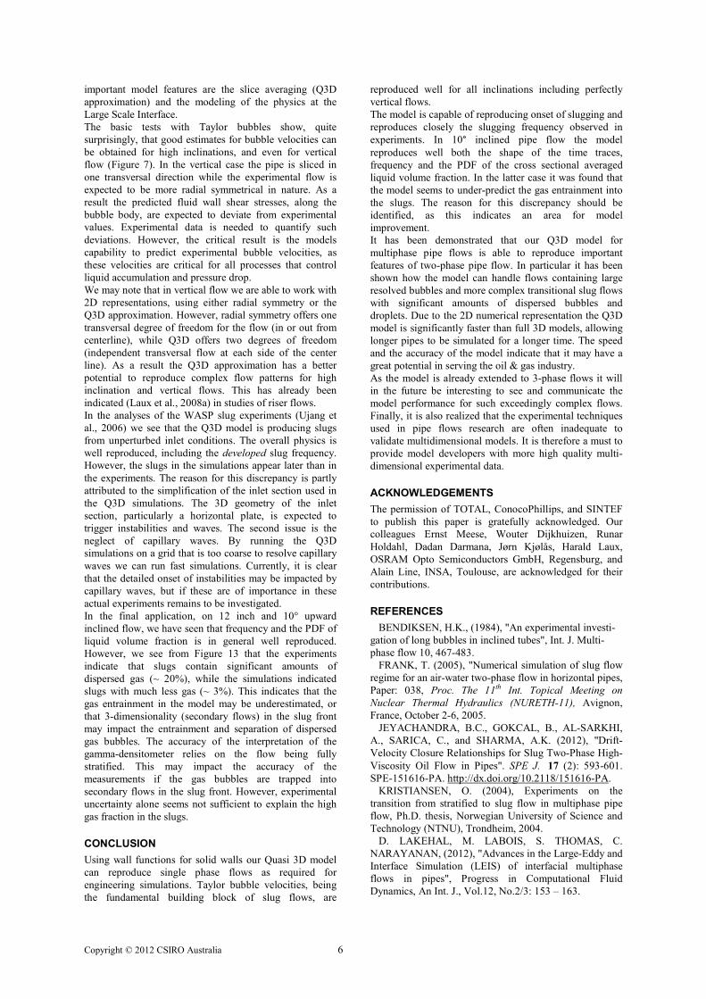
Figure 7: Comparison of Q3D results with experiments

(Zukowski 1966) and correlation (Bendiksen 1984).

SLUG FLOW APPLICATIONS

Horizontal flows

As we have demonstrated that the model well reproduces

both pressure drops and Taylor bubble slip velocities, we

now look into the reproduction of slug flow. The

numerical simulation described for this case is based on

experiments carried out at Imperial College London

(WASP facility) by Ujang et al. (2005) in order to study

the initiation and the subsequent evolution of

hydrodynamic slugs in a horizontal pipe. Air-water

experiments were carried out at atmospheric pressure, 4.0

bar(a) and 9.0 bar(a), and the effects of superficial liquid

and gas velocities were investigated. The test section used

for these experiments was 37 m in length, with an internal

diameter of 0.078 m. Further details are described in the

paper.

For the numerical simulation presented here, atmospheric

pressure with Usg = 4.64 m/s and Usl = 0.611 m/s were

used. The pipe length was 30 m with 10�2440 cells

uniformly distributed across the diameter of the pipe and

in the axial direction, respectively, leading to a grid aspect

ratio of 1.5. Gas compressibility was taken into account by

using a PVT table created for the air-water system. No

perturbations were imposed at the inlet so that fluid phases

were entering the pipe fully stratified. The details of the

inflow arrangement for the fluids were not included in the

simulations. The pipe was initially filled with stratified air

and water with 50-50 volume percentage and zero

velocity. Computations were carried out in parallel on 4

CPUs using MPI. The total flow time for this simulation

was 52.7 seconds for which a total clock time of 2.3 days

was used2.

Snapshots from the evolution of slugs in the pipe are

shown in Figure 8. The pipe diameter is magnified 5 times

for clarity of the flow details. Initially the water phase is

smooth and it takes some simulation time until a first wave

is created, growing to a slug which blocks the cross

section of the pipe (frame a) and grows in size as it

progresses in the pipe. However, this initial long slug

(frames c-e) is not periodic and is believed to be generated

out of the initial condition of the flow inside the pipe.

Similar initial slugs are also observed in experiments, e.g.

Kristiansen (2004).

Figure 8: Snapshots of Q3D results showing the time

evolution of slugs in a 30 m long horizontal pipe (diameter

is magnified 5 times). Here red is liquid and blue is gas.

Flow is from left to right.

After that the initial long slug has almost drained the pipe

from liquid (frame f), the interface level starts to rise until

it reaches a critical level (frame h) at which interfacial

disturbances are created and next grow into a new slug

(frame j). These disturbances are captured by the model,

and as the simulation proceeds further in time, they grow

into slugs which completely block the cross section of the

2 For a comparison with full 3D simulation we note that

Lakehal et al. (2012) using the TransAt code used 21 days

on 8 cores to run 16 m pipe for 30 seconds real time. The

mesh had 1.4 million cells. Their results were better in

predicting the slug frequencies the first 5-10 m in the pipe,

but had larger errors than Q3D later.


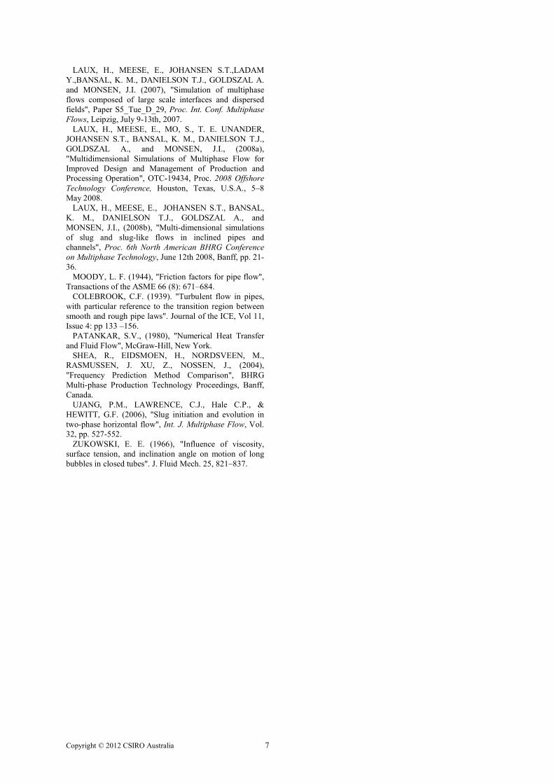
pipe. Figure 9 shows the liquid hold-up time series at

different probe locations along the pipe. The development

of slug flow in space and time can be studied in great

detail. The frequency of the slugs is calculated from these

time series based on both 60% and 80% volume fraction

of liquid phase as a defined threshold for the slug. The

calculated frequency versus distance from the inlet is

plotted in Figure 10 and compared with the experimental

values. In the experiments, a high frequency of slugs

formed in the inlet region of the pipe is observed. This

effect is not captured by the model with the current inlet

and initial conditions. However, this is believed to be

strongly affected by the inlet conditions in the experiments

(Ujang, et al., 2005). At distances further from the inlet,

the slug frequency compares relatively well with

experiments.

Figure 9: Liquid hold-up time-series for hydrodynamic

slug flow at different locations (X [m]) along the

horizontal pipe. Vertical axis is shifted by 1.0 for each

series for readability.

Figure 10: Slug frequency variation along the pipe.

Inclined flows

In this section the Q3D model is applied to simulate flow

of oil/gas mixtures in a 12 inch and 10° upward inclined

pipe. The simulation results are compared to experimental

data obtained in the large scale loop at the SINTEF

multiphase flow laboratory. Simulation results are

presented and discussed for only one of the many 12 inch

experiments. More simulation cases for different

experiments in the 12 inch loop are presented and

discussed in Laux et al. (2007).

The used fluids reasonably represent a produced oil-gas

fluid system. The data on the physical properties, however,

is proprietary and can therefore not be given here. The

superficial velocities were Usg = 2.552 m/s and Usl =

0.502 m/s.

The simulations were performed using a compressible gas

on a 100 m pipe on a 20�2000 grid3. A typical flow

situation is shown in Figure 11. Here we see one slug

bridging the pipe fully, while some large waves are about

to bridge the pipe. The turquoise color shows regions

where unresolved gas bubbles have been entertained into

the liquid (blue). The entrainment of gas bubbles is seen to

be more intense at the slug fronts. In Figure 12 we

compare time traces of liquid hold-up from simulations

and experiments. The main behavior is very similar, but

the amplitude is somewhat larger in the simulated results.

The corresponding probability density function (PDF) is

shown in Figure 13. The main peak is almost exactly at

the same volume fraction. The shape of the PDF indicates

slug flow since we have two "peaks" even if the high hold-

up peak is not very pronounced.

Figure 11: Excerpt of snap-shot from prediction of slug

flow in an inclined pipe, 12 inches in diameter and 100 m

long (the pipe diameter in the picture is magnified 5

times). The colours denote gas fraction, where red is 100%

gas and deep blue is no gas (liquid). Flow is from left to

right.

Figure 12: Liquid hold-up signal at a location 90 meters

from the pipe inlet as compared to the experimental

Gamma-ray signals.

Figure 13: Probability density function (PDF) of the

liquid volume fraction (VF) signal at 90 m from inlet

compared with that of experimental data.

DISCUSSION

The Q3D model is, as described above, built on several

simplifications and sub-scale models. The two most

3 The simulation time needed to run this case on 8

processors for 3 min real time was about 3.5 days.


important model features are the slice averaging (Q3D

approximation) and the modeling of the physics at the

Large Scale Interface.

The basic tests with Taylor bubbles show, quite

surprisingly, that good estimates for bubble velocities can

be obtained for high inclinations, and even for vertical

flow (Figure 7). In the vertical case the pipe is sliced in

one transversal direction while the experimental flow is

expected to be more radial symmetrical in nature. As a

result the predicted fluid wall shear stresses, along the

bubble body, are expected to deviate from experimental

values. Experimental data is needed to quantify such

deviations. However, the critical result is the models

capability to predict experimental bubble velocities, as

these velocities are critical for all processes that control

liquid accumulation and pressure drop.

We may note that in vertical flow we are able to work with

2D representations, using either radial symmetry or the

Q3D approximation. However, radial symmetry offers one

transversal degree of freedom for the flow (in or out from

centerline), while Q3D offers two degrees of freedom

(independent transversal flow at each side of the center

line). As a result the Q3D approximation has a better

potential to reproduce complex flow patterns for high

inclination and vertical flows. This has already been

indicated (Laux et al., 2008a) in studies of riser flows.

In the analyses of the WASP slug experiments (Ujang et

al., 2006) we see that the Q3D model is producing slugs

from unperturbed inlet conditions. The overall physics is

well reproduced, including the developed slug frequency.

However, the slugs in the simulations appear later than in

the experiments. The reason for this discrepancy is partly

attributed to the simplification of the inlet section used in

the Q3D simulations. The 3D geometry of the inlet

section, particularly a horizontal plate, is expected to

trigger instabilities and waves. The second issue is the

neglect of capillary waves. By running the Q3D

simulations on a grid that is too coarse to resolve capillary

waves we can run fast simulations. Currently, it is clear

that the detailed onset of instabilities may be impacted by

capillary waves, but if these are of importance in these

actual experiments remains to be investigated.

In the final application, on 12 inch and 10° upward

inclined flow, we have seen that frequency and the PDF of

liquid volume fraction is in general well reproduced.

However, we see from Figure 13 that the experiments

indicate that slugs contain significant amounts of

dispersed gas (~ 20%), while the simulations indicated

slugs with much less gas (~ 3%). This indicates that the

gas entrainment in the model may be underestimated, or

that 3-dimensionality (secondary flows) in the slug front

may impact the entrainment and separation of dispersed

gas bubbles. The accuracy of the interpretation of the

gamma-densitometer relies on the flow being fully

stratified. This may impact the accuracy of the

measurements if the gas bubbles are trapped into

secondary flows in the slug front. However, experimental

uncertainty alone seems not sufficient to explain the high

gas fraction in the slugs.

CONCLUSION

Using wall functions for solid walls our Quasi 3D model

can reproduce single phase flows as required for

engineering simulations. Taylor bubble velocities, being

the fundamental building block of slug flows, are

reproduced well for all inclinations including perfectly

vertical flows.

The model is capable of reproducing onset of slugging and

reproduces closely the slugging frequency observed in

experiments. In 10° inclined pipe flow the model

reproduces well both the shape of the time traces,

frequency and the PDF of the cross sectional averaged

liquid volume fraction. In the latter case it was found that

the model seems to under-predict the gas entrainment into

the slugs. The reason for this discrepancy should be

identified, as this indicates an area for model

improvement.

It has been demonstrated that our Q3D model for

multiphase pipe flows is able to reproduce important

features of two-phase pipe flow. In particular it has been

shown how the model can handle flows containing large

resolved bubbles and more complex transitional slug flows

with significant amounts of dispersed bubbles and

droplets. Due to the 2D numerical representation the Q3D

model is significantly faster than full 3D models, allowing

longer pipes to be simulated for a longer time. The speed

and the accuracy of the model indicate that it may have a

great potential in serving the oil & gas industry.

As the model is already extended to 3-phase flows it will

in the future be interesting to see and communicate the

model performance for such exceedingly complex flows.

Finally, it is also realized that the experimental techniques

used in pipe flows research are often inadequate to

validate multidimensional models. It is therefore a must to

provide model developers with more high quality multi-

dimensional experimental data.

ACKNOWLEDGEMENTS

The permission of TOTAL, ConocoPhillips, and SINTEF

to publish this paper is gratefully acknowledged. Our

colleagues Ernst Meese, Wouter Dijkhuizen, Runar

Holdahl, Dadan Darmana, Jørn Kjølås, Harald Laux,

OSRAM Opto Semiconductors GmbH, Regensburg, and

Alain Line, INSA, Toulouse, are acknowledged for their

contributions.

REFERENCES

BENDIKSEN, H.K., (1984), "An experimental investi-

gation of long bubbles in inclined tubes", Int. J. Multi-

phase flow 10, 467-483.

FRANK, T. (2005), "Numerical simulation of slug flow

regime for an air-water two-phase flow in horizontal pipes,

Paper: 038, Proc. The 11th Int. Topical Meeting on

Nuclear Thermal Hydraulics (NURETH-11), Avignon,

France, October 2-6, 2005.

JEYACHANDRA, B.C., GOKCAL, B., AL-SARKHI,

A., SARICA, C., and SHARMA, A.K. (2012), "Drift-

Velocity Closure Relationships for Slug Two-Phase High-

Viscosity Oil Flow in Pipes". SPE J. 17 (2): 593-601.

SPE-151616-PA. http://dx.doi.org/10.2118/151616-PA.

KRISTIANSEN, O. (2004), Experiments on the

transition from stratified to slug flow in multiphase pipe

flow, Ph.D. thesis, Norwegian University of Science and

Technology (NTNU), Trondheim, 2004.

D. LAKEHAL, M. LABOIS, S. THOMAS, C.

NARAYANAN, (2012), "Advances in the Large-Eddy and

Interface Simulation (LEIS) of interfacial multiphase

flows in pipes", Progress in Computational Fluid

Dynamics, An Int. J., Vol.12, No.2/3: 153 – 163.


LAUX, H., MEESE, E., JOHANSEN S.T.,LADAM

Y.,BANSAL, K. M., DANIELSON T.J., GOLDSZAL A.

and MONSEN, J.I. (2007), "Simulation of multiphase

flows composed of large scale interfaces and dispersed

fields", Paper S5_Tue_D_29, Proc. Int. Conf. Multiphase

Flows, Leipzig, July 9-13th, 2007.

LAUX, H., MEESE, E., MO, S., T. E. UNANDER,

JOHANSEN S.T., BANSAL, K. M., DANIELSON T.J.,

GOLDSZAL A., and MONSEN, J.I., (2008a),

"Multidimensional Simulations of Multiphase Flow for

Improved Design and Management of Production and

Processing Operation", OTC-19434, Proc. 2008 Offshore

Technology Conference, Houston, Texas, U.S.A., 5–8

May 2008.

LAUX, H., MEESE, E., JOHANSEN S.T., BANSAL,

K. M., DANIELSON T.J., GOLDSZAL A., and

MONSEN, J.I., (2008b), "Multi-dimensional simulations

of slug and slug-like flows in inclined pipes and

channels", Proc. 6th North American BHRG Conference

on Multiphase Technology, June 12th 2008, Banff, pp. 21-

36.

MOODY, L. F. (1944), "Friction factors for pipe flow",

Transactions of the ASME 66 (8): 671–684.

COLEBROOK, C.F. (1939). "Turbulent flow in pipes,

with particular reference to the transition region between

smooth and rough pipe laws". Journal of the ICE, Vol 11,

Issue 4: pp 133 –156.

PATANKAR, S.V., (1980), "Numerical Heat Transfer

and Fluid Flow", McGraw-Hill, New York.

SHEA, R., EIDSMOEN, H., NORDSVEEN, M.,

RASMUSSEN, J. XU, Z., NOSSEN, J., (2004),

"Frequency Prediction Method Comparison", BHRG

Multi-phase Production Technology Proceedings, Banff,

Canada.

UJANG, P.M., LAWRENCE, C.J., Hale C.P., &

HEWITT, G.F. (2006), "Slug initiation and evolution in

two-phase horizontal flow", Int. J. Multiphase Flow, Vol.

32, pp. 527-552.

ZUKOWSKI, E. E. (1966), "Influence of viscosity,

surface tension, and inclination angle on motion of long

bubbles in closed tubes". J. Fluid Mech. 25, 821–837.

Documents

QUASI-3D MODELLING OF TWO-PHASE SLUG FLOW IN · PDF filethe slug flow regime in horizontal pipes is presented in the paper by Frank (2005). In general, the current two major modeling