Embed Size (px)
Citation preview

INSURANCE MATHEMATICS
TEPPO A. RAKKOLAINEN
1
2 TEPPO A. RAKKOLAINEN
Foreword
This lecture notes were written for an advanced level course on Insurance Mathematicsgiven at Abo Akademi University during spring term 2010. While best efforts to correct alltypos found during the lectures (many thanks for the students for pointing out the typos)have been made, the notes are still without doubt in very unpolished form.
The presentation relies most heavily on lecture notes [1] and textbook [6] with regardto most of Part 1 (dealing with mathematical finance), and on textbook [13] with regardto Parts 2 and 3 (dealing with classical life insurance mathematics and multiple statemodels, respectively). In Part 4, use has been made of several sources. References arenot explicitly given in the text of the presentation, as this to me seems not to be reallynecessary considering the purpose of lecture notes.
To conclude this foreword, a thought on studying and attending lectures from the Devil:
”Habt Euch vorher wohl prapariert,Paragraphos wohl einstudiert,Damit Ihr nachher besser seht,Dass er nichts sagt, als was im Buche steht.”
(Mephistopheles in Goethe’s Faust)
Turku, April 2010
Teppo Rakkolainen
Some minor corrections and additions were made in August 2013. TR
INSURANCE MATHEMATICS 3
Contents
Foreword 21. Some Financial Mathematics 51.1. Motivation: On the Role of Investment in Insurance Business 51.2. Financial Markets and Market Participants 61.3. Interest Rates 81.4. Spot and Forward Rates 131.5. Term Structure of Interest Rates 141.6. Annuities 151.7. Internal Rate of Return 201.8. Retrospective and Prospective Provisions; Equivalence Principle 221.9. Duration 241.10. Some Financial Instruments and Investment Opportunities 261.10.1. Loans 271.10.2. Money Market Instruments 281.10.3. Bonds 291.10.4. Stocks 341.10.5. Real Estate 381.10.6. Alternative Investments 391.11. Financial Derivatives 411.11.1. Forwards and Futures 411.11.2. Swaps 431.11.3. Options 461.12. Some Basics of Investment Portfolio Analysis 521.12.1. Utility and Risk Aversion 531.12.2. Portfolio Theory 541.12.3. Markowitz Model and Capital Asset Pricing Model 551.12.4. Portfolio Performance Measurement 591.12.5. Portfolio Risk Measurement 602. Life Insurance Mathematics: Classical Approach 622.1. Future Lifetime 622.2. Mortality 632.2.1. Mortality Models 662.2.2. Select Mortality and Cohort Mortality 672.2.3. Competing Causes of Death 672.3. Expected Present Values of Life Insurance Contracts 702.3.1. Mortality and Interest 702.3.2. Present Value of A Single Life Insurance Contract 712.3.3. Present Value of A Pension 732.3.4. Net Premiums 772.3.5. Multiple Life Insurance 792.4. Technical Provisions 82

4 TEPPO A. RAKKOLAINEN
2.4.1. Prospective Provision 832.4.2. Retrospective Provision 842.5. Thiele’s Differential Equation 852.5.1. Basic Form of Thiele’s Equation 852.5.2. Generalizations of Thiele’s Equation 862.5.3. Equivalence Equation 882.5.4. Premiums 892.5.5. Technical Provision 902.6. Expense Loadings 932.7. Some Special Issues in Life Insurance Contracts 942.7.1. Surrender Value and Zillmerization 952.7.2. Changes in Contract after Initiation 952.7.3. Analysis and Surpluses 963. Multiple State Models in Life Insurance 983.1. Transition Probabilities 983.2. Markov Chains 983.3. A Very Short Interlude on Linear Differential Equations 1013.4. Evolution of the Collective of Policyholders 1023.5. Solutions for Transition Probabilities 1033.6. An Example of a Disability Model 1064. On Asset–Liability Management 1104.1. Classical Asset-Liability Theory 1104.2. Immunization of Liabilities with Bonds 1114.3. Stochastic Asset–Liability Management 1144.4. On Market-Consistent Valuation and Stochastic Discounting 116References 118
INSURANCE MATHEMATICS 5
1. Some Financial Mathematics
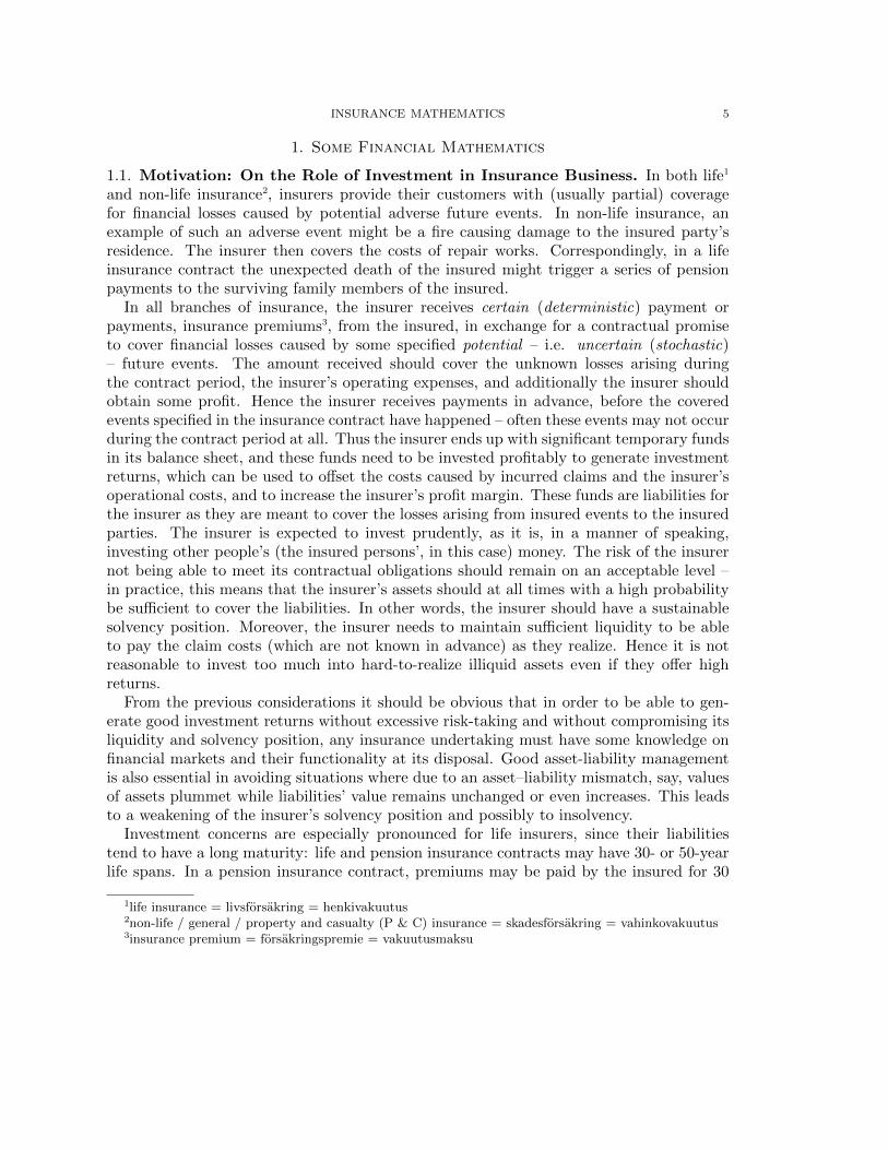
1.1. Motivation: On the Role of Investment in Insurance Business. In both life1
and non-life insurance2, insurers provide their customers with (usually partial) coveragefor financial losses caused by potential adverse future events. In non-life insurance, anexample of such an adverse event might be a fire causing damage to the insured party’sresidence. The insurer then covers the costs of repair works. Correspondingly, in a lifeinsurance contract the unexpected death of the insured might trigger a series of pensionpayments to the surviving family members of the insured.
In all branches of insurance, the insurer receives certain (deterministic) payment orpayments, insurance premiums3, from the insured, in exchange for a contractual promiseto cover financial losses caused by some specified potential – i.e. uncertain (stochastic)– future events. The amount received should cover the unknown losses arising duringthe contract period, the insurer’s operating expenses, and additionally the insurer shouldobtain some profit. Hence the insurer receives payments in advance, before the coveredevents specified in the insurance contract have happened – often these events may not occurduring the contract period at all. Thus the insurer ends up with significant temporary fundsin its balance sheet, and these funds need to be invested profitably to generate investmentreturns, which can be used to offset the costs caused by incurred claims and the insurer’soperational costs, and to increase the insurer’s profit margin. These funds are liabilities forthe insurer as they are meant to cover the losses arising from insured events to the insuredparties. The insurer is expected to invest prudently, as it is, in a manner of speaking,investing other people’s (the insured persons’, in this case) money. The risk of the insurernot being able to meet its contractual obligations should remain on an acceptable level –in practice, this means that the insurer’s assets should at all times with a high probabilitybe sufficient to cover the liabilities. In other words, the insurer should have a sustainablesolvency position. Moreover, the insurer needs to maintain sufficient liquidity to be ableto pay the claim costs (which are not known in advance) as they realize. Hence it is notreasonable to invest too much into hard-to-realize illiquid assets even if they offer highreturns.
From the previous considerations it should be obvious that in order to be able to gen-erate good investment returns without excessive risk-taking and without compromising itsliquidity and solvency position, any insurance undertaking must have some knowledge onfinancial markets and their functionality at its disposal. Good asset-liability managementis also essential in avoiding situations where due to an asset–liability mismatch, say, valuesof assets plummet while liabilities’ value remains unchanged or even increases. This leadsto a weakening of the insurer’s solvency position and possibly to insolvency.
Investment concerns are especially pronounced for life insurers, since their liabilitiestend to have a long maturity: life and pension insurance contracts may have 30- or 50-yearlife spans. In a pension insurance contract, premiums may be paid by the insured for 30
1life insurance = livsforsakring = henkivakuutus2non-life / general / property and casualty (P & C) insurance = skadesforsakring = vahinkovakuutus3insurance premium = forsakringspremie = vakuutusmaksu
6 TEPPO A. RAKKOLAINEN
years, after which the insured receives pension payments for 20 years. Matching assetsfor such long-term liabilities are not easily found from financial markets, and since termsof the contract are usually fixed in the beginning, the insurer may not be able to adjustpremiums to accommodate adverse developments. In contrast, non-life insurance contractsare usually renewed annually and the terms can be adjusted when contract is renewed.Hence the risk for an asset–liability mismatch is smaller.
Understanding of the workings of financial markets and the basic principles for valuationof financial assets is of fundamental importance for actuaries nowadays, since they havea responsibility not only to ensure appropriate and correct calculation of their company’sliabilities, but also to ensure that the company’s assets appropriately match these liabilitiesand that the company’s investment strategy takes properly into account the requirementsset by the nature of the liabilities. A total balance sheet approach and market consistentvaluation (of both assets and liabilities) are also central principles in the Solvency II Di-rective creating a new solvency regime and regulatory framework for all life and non-lifeinsurers in the E. U.
1.2. Financial Markets and Market Participants. Financial markets bring providersof capital together with the users of capital. Their function is to facilitate channeling offunds from savers to investors. In this role the markets complement the financial inter-mediaries (banks, insurance companies etc.) and compete with these institutions. On theother hand, financial institutions are also important players in financial markets.
Some major reasons for the existence of financial markets are the following:
(1) They enable consumption transfer over time;(2) They enable risk sharing, hedging and risk transfer among market participants;(3) They enable conversions of wealth;(4) They produce information and improve allocation of resources to most productive
uses.
Financial markets also provide fascinating opportunities for gamblers.An important concept central to much of the theory of mathematical finance is market
efficiency. In efficient markets, the market prices reflect all investors’ expectations giventhe set of available information. Prices of all assets equal their investment value at alltimes, and forecasting market movements or seeking undervalued assets based on availableinformation is futile: you cannot beat the market, which incorporates any new informationimmediately into prices. Put differently, investors cannot expect to make abnormal profitsby using the available information to formulate buying and selling decisions: they can onlyexpect a normal rate of return on their investments.
Market efficiency can be classified according to what information exactly is considered tobe fully reflected in market prices. In weak form efficiency, past price information cannotpredict future prices; in semi strong form efficiency, prices contain all publicly availableinformation; and in strong form efficiency prices contain all information, including insiderinformation.
An important aspect of markets is their liquidity (or lack of it). In a liquid market,an investor wishing to sell a security will always easily find a counterparty willing to
INSURANCE MATHEMATICS 7
buy the security at market price - an individual transaction has no impact on the price.Characteristic for deeply liquid markets is an abundance of ready and willing buyers andsellers so that market prices can be determined by demand and supply in the marketplace.In illiquid markets, this price discovery process does not operate due to a lack of ready andwilling buyers or sellers. In this sense illiquid markets cannot be efficient as the marketpricing mechanism does not work. Fundamentally illiquidity is due to investors’ uncertaintyabout the true value of a security. Importance of liquidity (it has been called “oxygen fora functioning market“, reflecting the fact that while it is available it is not really noticed,but a lack of it is immediately observable and has dire consequences) has been reinforcedby the recent financial crisis begun by the collapse of the U. S. subprime mortgage marketin 2007-2008.
One of the central areas of interest in mathematical finance is valuation or pricing ofassets. In this presentation we will later on consider valuation of some specific finan-cial assets in more detail. At this point we only point out that pricing methodologiescan broadly be classified into two groups: principles based on discounted cash flow andprinciples based on arbitrage-free valuation. The term arbitrage refers to an investmentopportunity providing risk-free (excess) returns, that is, certain profit without any risk –a money making automaton. Such an opportunity implies that there is a misalignmentof prices – someone is providing the “free“money without being compensated for this. Indeeply liquid efficient markets, no arbitrage opportunities should exist, as such oppor-tunities are constantly sought out by investors and taken advantage of as they appear,whereupon the price of the security in question goes up with increased demand until theprice misalignment which gave rise to the arbitrage has completely disappeared. In liq-uid efficient markets, this process is almost instantaneous as large sophisticated investorsmonitor markets continuously seeking arbitrage opportunities.
The most important submarkets of financial markets are
money market : where corporations and governments borrow short term by issuingsecurities with maturity less than a year;
bond market : where corporations and governments borrow long term by issuingbonds;
stock market : where corporations raise capital by issuing shares or stocks, certifi-cates conveying certain rights to their holders, and these shares are traded betweeninvestors in so-called secondary markets; and
derivative market : where financial derivatives, that is securities whose value is afunction of the values of some other securities (so-called underlying securities), aretraded, the most typical examples being options, forwards, futures and swaps.
In all the submarkets the ownership of securities can be transferred between investorsafter issuance through so-called secondary markets; however, the liquidity of secondarymarkets can vary considerably depending on the security. While stocks traded on anorganized exchange are typically highly liquid, bonds with very long maturities or exoticderivatives may be quite illiquid. Additionally, liquidity of a market is not constant in time– during periods of financial stress, markets previously considered liquid may “dry up“ and
8 TEPPO A. RAKKOLAINEN
become illiquid. Again, the subprime mortgage crisis provides an example: mortgage-backed securities with high credit ratings were quite liquid (there were willing buyers) aslong as the credit rating was believed to reflect the true value of the securities, but as itbecame clear that ratings were way out of line with actual reality, the investors’ uncertaintyconsidering the true value of these securities increased to the point causing almost totalilliquidity – there were virtually no willing buyers at all.
Market participants can broadly be classified into three groups: speculators try to ob-tain profits by making bets on the future direction of markets; arbitrageurs try to obtainprofits by taking advantage of inconsistencies in prices between different securities ; whilehedgers seek to reduce their risk exposures by taking positions on the market. Specula-tors and arbitrageurs play an important role in enhancing liquidity and efficiency of themarkets. They are the ones constantly monitoring the prices and processing information;their investment decisions then influence supply and demand which determine the marketprices.
1.3. Interest Rates. In a loan agreement, one party (the lender 4) loans a specified amountof money (the principal 5 of the loan) to another party (the borrower 6) for a specifiedtime period, during which the borrower repays the principal and makes some additionalcompensation payments to the lender. Interest7 is the compensation required by the lendersfor lending funds to borrowers. To make this precise:
Definition 1.2.1: Suppose that a sum of B0 euros is loaned by a lender to a borrowertoday, and it is agreed that the borrower pays the lender B1 > B0 euros one yearfrom now. Then B1 − B0 is the interest on this loan paid by the borrower. The(one-year or annual) interest rate on the loan is
r :=B1 −B0
B0
and the corresponding accumulation factor8 is
R := 1 + r.
More generally, r (resp. R) is an annual interest rate (resp. accumulation factor),if it holds that
Bt = (1 + r)tB0 = RtB0,
where the amount Bt is the value of the loan (the amount borrower owes to lender)at time t.
Interest rates are usually quoted in nominal terms. The real interest rate is determined asthe difference of the nominal interest rate and the inflation rate. In this presentation wewill mostly deal with nominal quantities, interest rates or other. It should be observed,
4lender = langivare = lainanantaja5principal = kapital = paaoma6borrower = lantagare = lainanottaja7interest = ranta = korko8accumulation factor = kapitaliseringsfaktor = korkotekija
INSURANCE MATHEMATICS 9
however, that inflation plays a very significant role in many branches of insurance, e.g.benefits of pension funds are often linked to consumer price indices or other quantitiesclosely related to inflation.
There are several reasons for why interest is required by the lenders:
(1) The lender foregoes the possibility to increase his/her consumption by the amounthe/she borrows to someone. In an inflationary environment, the purchasing powerof money erodes as time passes, so without additional compensation the lenderwould suffer a loss of purchasing power since the nominal amount of money he/shereceives at the end of the loan period is worth less in real terms than the nominalamount that he/she lent. Moreover, delaying consumption also means taking onthe risk of not being able to consume the amount delayed later.
(2) The lender could have invested the principal of the loan to some other investmentand would then have received corresponding returns from this investment: notobtaining these returns is a cost which should be compensated by the interest ofthe loan. Another way of saying this is that the loan is an investment for the lender,and interest payments by the borrower are the returns on this investment.
(3) There is a risk that the borrower defaults: i.e. is not able to pay back a part orall of his/her loan or interest payments. Hence a loan is a risky investment, andthe lender requires an additional compensation for the default risk he/she takes onwhen loaning money.
Returning briefly to Definition 1.2.1, observe that from the lender’s point of view, r isthe return and R the total return of the loan investment. For the lender, the loan tothe borrower is a financial asset generating positive returns (gains) in the form of interestincome. For the borrower, the loan is a financial liability generating negative returns(losses) in the form of interest payments.
The above list can be summarized succinctly by the time value of money : one euroreceived today is worth more than one euro received one year from today. In financialmathematics, this is formalized by the concept of present value9: the nominal value of acash flow received in the future is discounted10 to the present time with the appropriateinterest rate (discount rate). Discounting is done by multiplying the nominal value of thecash flow with a discount factor11 defined (as a function of the appropriate interest rate r)as
(1) v :=1
1 + r=
1
R.
Thus, if the prevailing one-year risk-free interest rate is r %, the present value of a cashflow consisting of K euros a year from today is vK = K
1+r . This reflects the fact that with
an initial investment of K1+r euros to an asset yielding the risk-free return r, any investor
can (without any risk, i.e. with certainty) obtain K euros a year from today. The converse
9present value = nuvarde = nykyarvo10discounting = diskontering = diskonttaus11discount factor = diskonteringsfaktor = diskonttaustekija
10 TEPPO A. RAKKOLAINEN
operation to discounting is called accumulation12 and the discount factor is the inverseof accumulation factor defined in Definition 1.2.1. More generally, given an appropriatediscount rate r, the discount factor for a cash flow of K euros which is realized at time tis vtK = K
(1+r)t .
Example: Suppose that an investor expects to receive a cash flow consisting of K =1000 euros each year at the end of the year for the next 4 years and that the risk-freeinterest rate is constant r = 0.03. The present value of this cash flow is
4∑t=1
K
(1 + r)t= K
4∑t=1
1
(1 + r)t= 1000 ·
(1
1.03+
1
1.032+
1
1.033+
1
1.034
)= 3717.10.
In practice, there are several different interest rates in financial markets. As interestrates reflect the return on investment required by the lenders, it is clear that interest ratesvary depending on the risk characteristics of the loan, such as the maturity time of theloan and creditworthiness of the borrower. To facilitate comparison between interest ratesof different maturities, rates are usually expressed as annualized rates.
Example: Suppose that an investor has two alternatives: with an investment of 100euros, the investor can obtain 120 euros in two years. The total return of this in-vestment is 120/100 = 120%, and hence the relative return is 20 %. Alternatively,the investor can obtain 110 euros in one year. The total return of this second invest-ment opportunity is 110/100 = 110%, and the relative return thus 10%. However,these returns are not directly comparable, since they have different maturities. Tocompare the attractiveness of these investments, we must convert the returns to an-nual returns. The annualized return r2 of the two-year investment is the solution ofequation 100(1 + r2)2 = 120, which is easily calculated to be r2 = 0.0954 = 9.54%.This can be directly compared to the return of the second investment (which isalready an annual return) and we see that the second opportunity is better, as itsannual return 10% > 9.54%, the annual return of the first opportunity.
Annualized interest rates or returns are indicated by adding ’(p. a.)’ (short for Latin perannum) after the quantity (e.g. 5 % (p. a.)).
So far we have considered so-called compound interest. Compound interest13 meansthat the accrued interest is calculated periodically and added to the principal: on the nextperiod, interest is earned not only on the original principal but also on the interest ofprevious periods. Of importance is the compounding frequency : that is, how often is theaccrued interest added to principal. Suppose the effective interest rate is r % (p. a.) . Ifinterest is added to principal m times a year, an initial principal of V0 euros will grow inn years to
(2) V (n) = (1 + r)nV0 =
(1 +
r(m)
m
)nmV0
12accumulation = kapitalisering, diskontering framat= korkouttaminen, prolongointi13compound interest = sammansatt ranta = koronkorko, yhdistetty korko
INSURANCE MATHEMATICS 11
euros, where
(3) r(m) = m[(1 + r)
1m − 1
]is the nominal interest rate compounded m times per year equivalent to effective annualrate r. It is an easy exercise to show that r(m) < r for m > 1. Interest rate r(m) is a simpleinterest rate. With simple interest14, interest is earned only on the principal, linearly withtime. In general, if simple interest of r % (p. a.) is paid to a principal of V0 euros, in tyears the invested capital increases to
(4) V (t) = (1 + rt)V0.
Example: A 6-month deposit of K euros with a simple interest rate r % (p. a.) growsduring the first month to (1 + r
12)K, during the first three months to (1 + r4)K and
by maturity 6 months to (1 + r2)K.
Correspondingly, we define the discount factor and the nominal accumulation factor formth fraction of a year as
(5) v(m) :=1
1 + r(m)
m
= (1 + r)−1m = v
1m
and
(6) R(m) := 1 +r(m)
m= (1 + r)
1m = R
1m
Suppose now that we let the compounding frequency m→∞ and define
(7) δ := limm→∞
r(m) = limm→∞
(1 + r)1m − (1 + r)0
1m
;
from which we see that δ is the derivative of function (1 + r)x at point x = 0. Hence,
(8) δ = ln(1 + r)⇔ eδ = 1 + r = R.
Hence the final value of an n-year investment of initial capital V0 earning interest r % (p.a.) with continuous compounding, i.e. when accrued interest is immediately (continuously)added to principal, is
(9) Vn = V0eδn.
Thus we see that when interest rate is r (p. a.) with continuous compounding, then thediscount factor
(10) v = e−δ.
Here δ is sometimes called the force of interest15.A hybrid of simple and compound interest is the interest rate used by Finnish banks
(so-called ”pankkikorko”), where complete years are calculated using compound interest
14simple interest = enkel ranta = yksinkertainen korko15force of interest = ranteintensitet = korkoutuvuus
12 TEPPO A. RAKKOLAINEN
but a fraction of a year is interpolated linearly with simple interest. For an investmentearning this interest, an initial capital V0 increases in t years to
(11) V (t) = (1 + r(t− btc)) (1 + r)btcV0,
where bxc is the largest integer less than or equal to x. Observe that there are differentday count basis conventions with regard to how the value of t− btc is transformed from anumber of calendar days into a real number; in the following example we use the Englishor actual/365 convention.
Example: Suppose that on 15.1.2010 a bank loans 150000 euros with annual interestrate rB = 0.03 and that the principal is repaid on 30.6.2011 with no intermediaterepayments. We calculate the bank’s expected interest income from this loan.Loan period T is one full year and 16 + 28 + 31 + 30 + 31 + 30 = 166 days, so thatT − bT c = 166
365 = 0.45479, and hence by equation (11) the bank’s expected interestincome is
V (T )− V (0) =
(1 + 0.03 · 166
365
)· 1.03 · 150000− 150000 = 6607.95.
Above we have considered the force of interest as constant in time. This can be gen-eralized to accommodate variation in time by allowing δ to be a non-constant function oftime.
Definition 1.2.2: Let δ : I → R be a piecewise continuous function on an intervalI ⊂ R+. Function δ is a force of interest, if there exists a piecewise differentiable,continuous function V : I → R such that
(12) V′(t) = δ(t)V (t)
for all t ∈ I \ N , where N is the set of points of discontinuity of δ and points ofnondifferentiability of V .V is called a provision.
It is a simple exercise to show that if δ is a force of interest on [a, b], then the provision attime t ∈ [a, b] is given by
(13) V (t) = exp
(∫ t
aδ(u)du
)· V (a).
Suppose that δ is a force of interest and that u = t0 < t1 < . . . < tn−1 < tn = t. By virtueof the additivity of integrals, the provision can in this case be written as
(14) V (t) = V (u) exp
(∫ t1
uδ(s)ds
)exp
(∫ t2
t1
δ(s)ds
). . . exp
(∫ t
tn−1
δ(s)ds
).
If δ is a constant δi on each interval (ti, ti+1), then this simplifies to
(15) V (t) = V (u) exp
(n−1∑k=0
δk(tk+1 − tk)
)= V (u)
n−1∏k=0
(1 + rk).tk+1−tk ,
INSURANCE MATHEMATICS 13
where rk = eδk − 1 is the annual interest rate corresponding to force of interest δk. Thepresent value of provision V (t) at time u < t is
(16) V (u) = V (t) exp
(−∫ t
uδ(s)ds
).
1.4. Spot and Forward Rates. Loans paying no intermediate interest or amortizationpayments, but only one single payment consisting of principal and interest at maturitytime are called zero-coupon loans. Interest rate required by the lenders on a (default-free)zero-coupon loan with maturity T > 0 years beginning from today is called the T -yearspot rate. Hence spot rates are determined by prices of zero-coupon securities: if the futureprice of a zero-coupon security at time T is PT , and the current price is P0, then the T -yearspot rate
(17) sT =
(PTP0
) 1T
− 1.
In other words, knowing the prices of zero-coupon loans for a set of maturities is equivalentto knowing the spot rates for these maturities.
Example: Suppose that a borrower can obtain a loan of P0 = 100000 euros byagreeing to pay back P2 = 104040 euros after 2 years. Then the two-year spot rate
s2 =(
104040100000
)1/2 − 1 = 0.02.
There are also loan contracts which begin at some specified time in the future, sayS > 0 years from now. Interest rate required by lenders on such a loan (with maturity T )is called the forward rate16 from T − S to T . If we assume that the markets are arbitrage-free (meaning that there are no possibilities to make certain excess returns over and abovethe risk-free rate of return), then forward rates are determined by spot rates, since to avoidarbitrage opportunities we must have
(1 + sT )TV0 = (1 + sT−S)T−S(1 + fT−S,T )SV0 ⇔ fT−S,T =
((1 + sT )T
(1 + sT−S)T−S
)1/S
− 1,
where sU is the U -year spot rate and fV,W is the forward rate for period [V,W ]. That is,our return must be equal irrespective of whether we make a T -year investment of V0 euroson the spot market today, or make a T −S-year investment of V0 euros on the spot marketplus enter a (forward) contract where we agree at time T − S to invest (1 + sT−S)T−SV0
euros for S years at current forward rate for that period.
Example: Suppose that we know the one-year and two-year spot rates s1 = 0.012and s2 = 0.021. Then the forward rate for an investment that will be made oneyear from now for a period of a year must be
f12 =(1 + s2)2
1 + s1− 1 =
1.0212
1.012− 1 = 0.030
in order to avoid arbitrage.
16forward rate = terminranta = termiinikorko
14 TEPPO A. RAKKOLAINEN
In general, given the spot rates sTi for an increasing sequence of maturity times Ti, i =0, 1, 2, . . . , N , the forward rates fTi,Tj , Ti < Tj , can be calculated from
(18) (1 + fTi,Tj )Tj−Ti =
(1 + sTj )Tj
(1 + sTi)Ti.
In the continuous time framework, we denote the continuous spot rate at time t withmaturity T by s(t, T ). For different maturity times Ti ≥ 0, where Ti < Ti+1, the marketprice of a zero-coupon unit security is
P (t, Ti) = e−(Ti−t)s(t,Ti).
Now, denoting the continuously compounded forward rate available at time t for borrowingat time Ti and repaying at time Tj by f(t, Ti, Tj), the fundamental arbitrage relation takesthe form
e(Tj−t)s(t,Tj) = e(Ti−t)s(t,Ti)e(Tj−Ti)f(t,Ti,Tj).
This implies that
(19) f(t, Ti, Tj) = − lnP (t, Tj)− lnP (t, Ti)
Tj − Ti.
The instantaneous forward rate at time t for borrowing at time Ti is defined as the limit
f(t, Ti) = limTj↓Ti
f(t, Ti, Tj) = − ∂
∂Ti[lnP (t, Ti)]
Integrating both sides and denoting Ti = T yields∫ T
tf(t, u)du = −
∫ T
t
∂
∂u[lnP (t, u)] du ⇔ lnP (t, T ) = −
∫ T
tf(t, u)du.
Comparison with P (t, T ) = e−(T−t)s(t,T ) shows that the continuous spot rate has the rep-resentation
s(t, T ) =1
T − t
∫ T
tf(t, u)du
in terms of the instantaneous forward rate. The continuous discount factor at time t withmaturity T and time to maturity T − t is hence
v(t, T ) = e−s(t;T )(T−t) = e−∫ Tt f(t,u)du.
1.5. Term Structure of Interest Rates. Spot rates for different maturities rU |U > 0form the term structure of interest rates17, i.e. interest rate as a function of maturity.In practice, the short end of this term structure curve is directly observable in the mar-ket (money market securities are usually zero-coupon instruments with no intermediatepayments before maturity) but spot rates for the long-term market are not immediatelyobservable as securities make intermediate interest payments (coupons). Assets used inderiving the term structure should belong to the same risk class, i.e. there are different
17term structure of interest rates = rantekurva = korkokayra, korkojen aikarakenne
INSURANCE MATHEMATICS 15
term structures for government securities (risk-free or default-free term structure) and cor-porate securities of differing default risk (for example, one term structure for AAA ratedcorporations and another term structure for BBB rated corporations).
Example: Suppose that the prices of 1, 2 and 3-year zero-coupon loans with unitprincipal are P1 = 0.9850, P2 = 0.9525 and P3 = 0.9285. Then the correspondingspot rates are
s1 =
(1
0.9850
)1/1
−1 = 0.015, s2 =
(1
0.9525
)1/2
−1 = 0.025, s3 =
(1
0.9685
)1/3
−1 = 0.035.
In the above example the term structure is upward sloping, i.e. spot rates for longermaturities are higher than spot rates for shorter maturities. This is usually the case,but the term structure may occasionally also be hump-shaped or downward sloping. Tounderstand why this is so, recall that any interest rate reflects the required investmentreturn of an asset. This required return can be decomposed into the following components:
(1) the required real return for the investment horizon, which can be considered toconsist of the one-year real risk-free interest rate and a term premium with respectto the one-year rate, which depends on the investment horizon;
(2) expected inflation over the investment horizon; and(3) a risk premium reflecting the additional return needed to compensate investor for
additional risks such as default risk and illiquidity risk.
Real return reflects how much the investor wants his purchasing power to increase incompensation for delaying consumption. The longer the delay, the larger the compensation,and hence the term premium increases with investment horizon. This is one reason for theusual upward sloping term structure.
In an inflationary environment, investors require a compensation equal to the expectedinflation over the investment horizon to shield them from the erosion of purchasing power.If expected inflation is constant, this leads to an upward shift of the whole term structure;however, should inflation expectations be lower in the long run than in the short term, thismay cause the term structure to have a humped or downward-sloping shape.
If an asset is subject to default risk (or any other additional risk), a risk premium on topof the risk-free real return and expected inflation is required to make the asset attractiveto investors. Magnitude of the default risk premium depends on the creditworthiness ofthe asset’s issuer and also on the general market sentiment (risk appetite). Risk premiumsfor a specific issuer may also differ depending on the investment horizon. In the aftermath(?) of the recent financial crisis the existence and significance of an illiquidity premiumcomponent in the risk premium have come into focus. One line of thought is that sucha premium tends to be negligible during “normal“times but can very rapidly increase inperiods of financial stress.
1.6. Annuities.
16 TEPPO A. RAKKOLAINEN
Definition 1.4.1: An annuity18 is a cash flow consisting of annual payments of equalmagnitude. If the annual payment is equal to one unit, we speak of unit annuity.
If the first payment occurs at time 0 (at beginning of period), the annuity is called a annuitydue19 and the present value of a n-year unit annuity is given by
(20) an| := 1 + v + v2 + . . .+ vn−1 =n−1∑i=0
vi,
where v = 11+r = 1
R is the discount factor. Corresponding accrued provision is
(21) sn| := R+R2 + . . .+Rn =n∑i=1
Ri.
Annuities due are typically encountered in insurance contracts: the first premium is paidbefore the insurance cover is in force.
If the first payment occurs at time 1 (at end of period), we speak of immediate annuity20,and the present value of a n-year unit annuity is given by
(22) an| := v + v2 + . . .+ vn =n∑i=1
vi.
Corresponding accrued provision is
(23) sn| := 1 +R+R2 + . . .+Rn−1 =n−1∑i=0
Ri
Immediate annuities are encountered in bank loans: amortization and interest paymentsare usually paid at the end of the payment period.
An annuity with infinite duration is called a perpetuity21. Present values of perpetuitiesare obtained as limits of previous expressions as n → ∞. Observe that the present valueand accrued provision for immediate annuity can be obtained from the present value andaccrued provision for annuity due via discounting:
(24) an| = v · an| and sn| = v · sn|.Conversely, these quantities for annuity due can be obtained from their counterparts forimmediate annuity via prolongation:
(25) an| = R · an| and sn| = R · sn|.For r 6= 0, we have the following expressions for the present values and accrued provisions
of annuities:
(i) : an| =1−vnr·v and a∞| =
1r·v , for r > 0;
18annuity = annuitet, tidsranta = annuiteetti, aikakorko19annuity due = annuitet pa forhand = etukateinen annuiteetti20immediate annuity = annuitet pa efterhand = jalkikateinen annuiteetti21perpetuity = paattymaton aikakorko/annuiteetti = oandlig tidsranta/annuitet
INSURANCE MATHEMATICS 17
(ii) : an| =1−vnr and a∞| =
1r , for r > 0;
(iii): sn| =Rn−1r·v ;
(iv): sn| =Rn−1r .
To prove the first part of (i), we use the formula for the value of a geometric sum:
an| =n−1∑i=0
vi =1− vn
1− v=
1− vn
1− 11+r
=1− vn1+r−1
1+r
=1− vn
r · 11+r
=1− vn
r · v.
The second part of (i) follows now easily by letting n→∞, since for r > 0 we have |v| < 1.To prove assertions (ii)-(iv) is left as an exercise.
In reality, payments are often made more frequently than annually. To accommodatethis, we generalize the definition of annuity as follows.
Definition 1.4.2: An annuity payable m times a year is a cash flow consisting ofpayments of equal magnitude made at equal intervals m times a year . If theindividual payment is equal to 1
m , we speak of a unit annuity.
The present value and accrued provision of an n-year unit annuity due payable m times ayear are
(26) a(m)n| :=
1
m
(1 + v(m) + v(m)2
+ . . .+ v(m)nm−1)
and
(27) s(m)n| :=
1
m
(R(m) +R(m)2
+ . . .+R(m)nm).
Similarly, the present value and accrued provision of an immediate n-year unit annuitypayable m times a year are
(28) a(m)n| :=
1
m
(v(m) + v(m)2
+ . . .+ v(m)nm)
and
(29) s(m)n| :=
1
m
(1 +R(m) +R(m)2
+ . . .+R(m)nm−1).
As previously, the corresponding values for unit perpetuities payable m times a year areobtained by letting n→∞ in the expressions above.
If r(m) 6= 0, then for unit annuities payable m times a year, the present values andaccrued provisions are
(i) : a(m)n| = 1−v(m)mn
r(m)·v(m) and a(m)∞| = 1
r(m)·v(m) , for r(m) > 0;
(ii) : a(m)n| = 1−v(m)mn
r(m) and a(m)∞| = 1
r(m) , for r > 0;
(iii): s(m)n| = R(m)nm−1
r(m)·v(m) ;
(iv): s(m)n| = R(m)mn−1
r(m) .
18 TEPPO A. RAKKOLAINEN
To prove the first part of (i), we proceed exactly as we did earlier with annual paymentschedule:
a(m)n| =
1
m
mn−1∑i=0
(v(m))i =1
m
1− v(m)mn
1− v(m)=
1
m
1− v(m)mn
1− 1
1+ r(m)
m
=1− v(m)mn
r(m)v(m).
The second assertion of (i) follows again by letting n → ∞. To show the validity of theremaining formulas is left as an exercise.
Sometimes it is necessary to define annuities for durations other than integer multiplesof period 1
m . This can be achieved nicely using the indicator function
I[0,n)(t) =
1, t ∈ [0, n)
0, otherwise.
An n-year annuity due payable m times a year can be expressed using indicator functionsas
a(m)n| =
1
m
∞∑k=0
v(m)kI[0,n)
(k
m
).
Suppose now that t > 0 (i.e. t is not necessarily an integer). The present value of a t-yearannuity due payable m times a year is
a(m)
t| =1
m
∞∑k=0
v(m)kI[0,t)
(k
m
),
and the present value of a t-year immediate annuity payable m times a year is
a(m)
t| =1
m
∞∑k=0
v(m)kI(0,t]
(k
m
).
An annuity with continuous payments is obtained by letting the number of subperiodsm → ∞. In this case there is no difference between the cash flows of annuity due and ofimmediate annuity. We define a continuous cash flow as a generalization of the differentialequation for provision in Definition 1.2.2. In order to do this, define the continuous timediscount factor
(30) v(u, t) := exp
(−∫ t
uδ(v)dv
)and the continuous time accumulation factor
(31) R(u, t) := exp
(∫ t
uδ(v)dv
),
where the force of interest δ is a piecewise continuous function.
INSURANCE MATHEMATICS 19
Definition 1.4.3: A continuous cash flow paid into a continuous and piecewise dif-ferentiable provision V is a piecewise continuous mapping b defined on some interval[0, T ] such that the differential equation
(32) V′(t) = δ(t)V (t) + b(t)
is satisfied piecewise, at every point of continuity of functions δ and b on [0, T ].
The present value of a t-year continuous cash flow at time t0 is
(33)
∫ t
t0
b(u)v(t0, u)du.
A continuous t-year unit annuity is a t-year continuous constant unit cash flow (i.e. b(u) ≡1). Its present value is
(34) at|(δ) :=
∫ t
0v(0, u)du.
and its accrued provision at time t is
(35) st|(δ) :=
∫ t
0R(u, t)du.
For a constant force of interest δ
(36) at| =
∫ t
0e−δudu =
1− e−δt
δ=
1− vt
δ
and
(37) st| =
∫ t
0eδ(t−u)du = eδt
1
δ
(1− eδt
)=Rt − 1
δ.
For a continuous cash flow, the provision at time t ∈ [0, T ] is
(38) V (t) = R(0, t)
(V (0) +
∫ t
0b(u)v(0, u)du
).
To see this, observe that the right side of equation (38) is the solution of the first orderdifferential equation (32), when using the notations given in (30) and (31). Furthermore,for a continuous unit annuity with initial provision V (0) = 0, we have
(39) V (t) = R(0, t)at|(δ),
i.e. provision is the prolongated present value of the annuity, and conversely,
(40) at|(δ) = v(0, t)st|(δ),
i.e. the present value of the annuity is the discounted value of the provision. To see this,observe that for V (0) = 0 and b(u) ≡ 1, the equation (38) takes the form
(41) V (t) = R(0, t)
(∫ t
0v(0, u)du
)= R(0, t)at|(δ),
20 TEPPO A. RAKKOLAINEN
while(42)
at|(δ) =
∫ t
0v(0, u)du = v(0, t)
∫ t
0R(0, t)v(0, u)du = v(0, t)
∫ t
0R(u, t)du = v(0, t)st|(δ).
Payments of an annuity are often linked to some index (e.g. a consumer price index).Assuming the index value increases periodically by 100 · k %, the corresponding accumu-
lation factor is Rk = 1 + k and the jth payment Bj = RjkB, where B is the first payment.Accrued provision for such a geometrically increasing annuity is
n−1∑j=0
Rn−jBj =n−1∑j=0
Rn−jRjkB = B ·RRn −RnkR−Rk
= B ·RRn −Rnkr − k
,
provided that r 6= k and the present value is
n−1∑j=0
vjBj =n−1∑j=0
vjRjkB = BvnRnk − 1
vRk − 1= BR1−nR
n −Rnkr − k
.
Denote κ = ln(1 + k). For a continuous geometrically increasing annuity with a constantforce of interest δ 6= κ the accrued provision is
B
∫ t
0eδ(t−u)eκudu = Beδt
e(κ−δ)t − 1
κ− δ= B
eκt − eδt
κ− δand the present value is
B
∫ t
0e−δueκudu = B
e(κ−δ)t − 1
κ− δ= Be−δt
eκt − eδt
κ− δ.
For δ = κ, the corresponding values are equal to t · eδt ·B and t ·B, respectively.
1.7. Internal Rate of Return. Assume that we know the cash flow B(ti), where thepayment times t1 < t2 < . . . are not necessarily evenly spaced, and also we know eitherS(t), the provision accrued up to time t > t1, or A(t), the present value of payments dueup to time t. The internal rate of return22 for the considered cash flow is the constantannual interest rate rIRR satisfying either
(43) S(t) =∑tj<t
B(tj)(1 + rIRR)t−tj
or
(44) A(t) =∑tj<t
B(tj)(1 + rIRR)−tj .
In general (and usually in practice), rIRR cannot be solved algebraically from previousequations: since time is usually measured in discrete units (day, month, year), these equa-tions are real polynomials, possibly of high degree. The number of solutions (which may becomplex numbers) is then equal to the degree of the polynomial. Numerical methods are
22internal rate of return = internranta = sisainen korko(kanta)
INSURANCE MATHEMATICS 21
hence usually needed if there are more than four23 payment times or if the payment timesare unequally spaced. We are interested in real-valued solutions rIRR such that rIRR > −1.Since S(t) = RtA(t), it suffices to consider equation (43).
Example: Consider the following provision: at time 0, a sum of 100 euros is loanedfrom the provision, at time 1 a sum of 230 euros is paid to the provision and atmaturity, time 2, the provision of 132 euros is paid out. In this case the equationfor accrued provision in terms of accumulation factor R = 1 + r is
−100 ·R2 + 230 ·R− 132 = 0.
This second degree polynomial has 2 roots, R = 1.1, 1.2. i.e. we have twosolutions rIRR = 10% or rIRR = 20%.
Several real solutions larger than −1 may appear if there are alternating positive andnegative cash flows. However, the following result tells us when a unique solution exists.
Proposition: Suppose t1 < . . . < tn ≤ t. Equation (43) (and consequently alsoequation (44)) has a solution R = 1 + rIRR with rIRR > −1, if S(t) ≥ 0 andB(t1) > 0. Furthermore, this solution is unique, if the provision is positive aftereach payment, that is,
(45) S(t) =∑tj<tk
B(tj)(1 + rIRR)tk−tj > 0, for each k = 1, . . . , n.
Proof: Denote
(46) V (t, r) :=∑tj<t
B(tj)(1 + r)t−tj
and consider solving V (t, r) = S(t) for r. Observe that V is a continuous functionof r, and that V (t,−1) = 0 and limr→∞ V (t, r) = ∞, since by assumptions madet > t1 and B(t1) > 0. Hence S(t) ≥ 0 implies that a solution exists.
To prove uniqueness under the additional assumption (45), suppose that there
would exist two distinct solutions r′> r > −1. Then the following chain of
inequalities holds:∑nj=1B(tj)(1 + r)t−tj = (1 + r)t−tn
(∑n−1j=1 B(tj)(1 + r)tn−tj +B(tn)
)< (1 + r
′)t−tn
(∑n−1j=1 B(tj)(1 + r)tn−tj +B(tn)
)< (1 + r
′)t−tn
((1 + r
′)tn−tn−1
(∑n−2j=1 B(tj)(1 + r)tn−1−tj +B(tn−1)
)+B(tn)
)<∑n
j=1B(tj)(1 + r′)t−tj = S(t),
but then either r or r′
is not a solution. Hence the solution is unique.
In practice, we often have the situation in which the first k payments are positive and theremaining n − k payments are negative. If S(tn) = 0, then the provision has a uniqueIRR: by the previous proposition, IRR exists, and by construction the provision must bepositive after each payment since the final value S(tn) = 0.
23Polynomials of degree d > 4 do not have general solution formulas.
22 TEPPO A. RAKKOLAINEN
Example: Consider the cash flow where for 10 years a payment of 5 units is madeat year end to a provision and after this for 5 years 12 units are taken out at theend of each year. If we wish to know what interest rate the provision should earnin order for it to be just sufficient to cover all the payments, we need to calculatethe IRR of the cash flow with assumption that final provision S(15) = 0. That is,we need to solve
5 ·10∑t=1
(1 + r)15−t − 12 ·15∑t=11
(1 + r)15−t = 0.
for r. Solving this numerically with Excel yields rIRR = 2.436 %. So this IRR is theinterest rate the provision must earn in order for it to be sufficient to finance theoutgoing payments during last 5 years. This example represents in simplified formthe usual situation in a life or pension insurance contract where first premiums arepaid by the insured for a specified period of time and after this the insured receivespension payments for a specified period of time.
Example: Suppose that a firm has estimated that the building of a new productionplant would lead to the following cash flow of annual profit/loss:
B = −100,−150,−50,−50, 0, 10, 30, 50, 90, 120, 150, 120, 100, 100, 100,
where in the first years the costs of building cause total cash flow to be negativebut eventually as the new plant is finished, new products can be produced andsold, and the cash flow becomes positive. In the final years the plant is becomingobsolete and maintenance costs rise; last cash flow B15 represents the scrap value ofthe plant as it is sold, and hence the “provision“at the end of investment project iszero, S(15) = 0. The firm can now compute the IRR of the project from equation
15∑t=1
Bt(1 + r)15−t = 0.
, which is (using Excel) rIRR = 10.519 %.
By calculating the internal rate of return we can compare cash flows with different paymenttimes and maturities.
1.8. Retrospective and Prospective Provisions; Equivalence Principle. Considera provision S(t) defined for t ∈ [0, n] with a force of interest δ(t) and receiving a continuouscash flow b(t) which can take both positive and negative values. Dynamics of this provisionare described by the differential equation
(47) S′(t) = δ(t)S(t) + b(t).
If the initial provision S(0) is known, the provision is
(48) S(t) = R(0, t)
(S(0) +
∫ t
0b(u)v(0, u)du
).
INSURANCE MATHEMATICS 23
As the provision is here expressed in terms of the past (before time t), it is called theretrospective provision.
Alternatively, the final provision S(n) can be solved from equation (47) in terms ofprovision S(t) (known at time t):
(49) S(n) = R(t, n)
(S(t) +
∫ n
tb(u)v(t, u)du
).
From this, we can solve S(t):
(50) S(t) = v(t, n)S(n)−∫ n
tb(u)v(t, u)du.
The provision calculated in terms of future (after time t) is called the prospective provision.The future is known via the contract concerning the provision, which specifies the finalvalue, the future cash flow payments and the interest to be paid.
If the force of interest δ is constant and the cash flow b(t) differs from 0 only at discretepoints 0 = t1 < t2 < . . . < tm, taking values B(tj), j = 1, . . . ,m, then
(51) S(t) = Rt
S(0) +∑ti≤t
vtiB(ti)
= RtS(0) +∑ti≤t
Rt−tiB(ti)
and
(52) S(t) = vn−tS(n)−∑ti≥t
vti−tB(ti).
Put verbally, the retrospective provision equals initial provision and paid payments withaccrued interest, while the prospective provision is the difference between the final provisionand the present value of future payments. Retrospective and prospective provision arenaturally equal, being solutions of the same differential equation.
Two cash flows are equivalent, if their present values are equal under a common interestrate assumption. If the present values of two cash flows, each calculated with a differentinterest rate, are equal at time t, then the cash flows are equivalent at time t. Equivalenceprinciple refers to matching two cash flows in such a way that they are equivalent at somespecified moment of time.
Example: Consider an annuity paying K units at each year end for n years. Thecontract stipulates that the applied discount rate may be changed during the con-tract period, in which case the amount of annual payment is adjusted in accordancewith the equivalence principle. The prevailing discount rate at the beginning of then year period is r1. Suppose that after the first year and payment the interest ratechanges to r2. Then the new annual payment K ′ satisfies
Kn−1∑t=1
vt1 = K ′n−1∑t=1
vt2,
24 TEPPO A. RAKKOLAINEN
which is equivalent to
K ′ =K · an−1|(r1)
an−1|(r2).
In general, given discount factors vi and payments Bi(tij), i = 1, 2 and ji = 1, 2, . . . ,mi,
where i = 1 is before the change and i = 2 is after the change, to satisfy the equivalenceprinciple we must have
m1∑j=1
vt1j1 B1(t1j ) =
m2∑j=1
vt2j2 B2(t2j ).
For continuous payments and forces of interest this becomes∫ n1
tb1(u)vδ1(t, u)du =
∫ n2
tb2(u)vδ2(t, u)du.
1.9. Duration. It is obvious that the present value of a cash flow depends on the applieddiscount rate. As interest rates on the markets are not constant in time, it is important toknow how the present value of a cash flow changes when the discount rate changes. Thiscan be measured with duration.
Definition 1.7.1: Let B(t) be a cash flow and δ the force of interest. Duration ofB(t) is
(53) D(δ) :=
∫∞0 t · vtB(t)dt∫∞
0 vtB(t)dt=: E(T ),
where v = e−δ and T is a random variable whose density function is
(54) fT (t) =vtB(t)∫∞
0 vuB(u)du.
If B(t) is a continuous cash flow, the integral is interpreted as a Riemann integralover the lifetime of the cash flow; if B(t) is a discrete cash flow, the integral isinterpreted as a sum over payment times with nonzero cash flow.
Duration of a cash flow is a weighted average of the cash flow’s payment times where theweights are the present values of payments. For a discrete cash flow B(ti), i = 1, . . . , n,with known payment times and magnitudes of payments, duration equals
(55) D(δ) =
∑nj=1 tjv
tjB(tj)∑nj=1 v
tjB(tj),
Observing that in this case e−δ = e− ln(1+r) = 11+r , we can write this also as a function of
the discount rate r as
(56) D(r) := D (ln(1 + r)) =
∑nj=1 tj
B(tj)
(1+r)tj∑nj=1
B(tj)
(1+r)tj
.
INSURANCE MATHEMATICS 25
Denote now by P (B, δ) the present value of cash flow B with a force of interest δ. The(infinitesimal) relative change in the present value of the cash flow due to a (infinitesimal)change in the force of interest δ is
(57)1
P (B, δ)
∂P (B, δ)
∂δ.
We have the following result:
(58) D(δ) = − 1
P (B, δ)
∂P (B, δ)
∂δ.
This follows easily by observing that
∂P (B, δ)
∂δ=
∂
∂δ
[∫ ∞0
e−δtB(t)dt
]= −
∫ ∞0
t · e−δtB(t)dt,
which combined with the definition of duration in (53) implies (58). (Provided, of course,that interchanging the order of integration and differentiation is allowed. In practicalapplications this is nearly always the case.) Hence for a small change ∆δ in the force ofinterest δ, we have an approximation for the corresponding relative change in the presentvalue of cash flow B:
(59)∂P (B, δ)
P (B, δ)= −D(δ)∂δ ⇒ ∆P (B, δ)
P (B, δ)≈ −D(δ)∆δ.
This approximation is a widely used application of the duration concept.We can also consider the sensitivity of duration D(δ) to changes in the force of interest
δ:∂D(δ)∂δ = ∂
∂δ
[∫∞0 tvtB(t)dt∫∞0 vtB(t)dt
]= 1∫∞
0 vtB(t)dt· ∂∂δ
[∫∞0 tvtB(t)dt
]−
∫∞0 tvtB(t)dt
(∫∞0 vtB(t)dt)
2 · ∂∂δ[∫∞
0 vtB(t)dt]
=−
∫∞0 t2vtB(t)dt∫∞0 vtB(t)dt
+(∫∞0 tvtB(t)dt)
2
(∫∞0 vtB(t)dt)
2 = D(δ)2 − E(T 2).
So we see that in terms of the random variable T defined in Definition 1.7.1, we have
(60)∂D(δ)
∂δ= D(δ)
2 − E(T 2) = −V ar(T ).
We can also consider duration as a function of the interest rate r according to equation(56). In this case the relative change of the value of cash flow B due to a change in theinterest rate r is
(61)1
P (B, r)
∂P (B, r)
∂r=∂δ
∂r
1
P (B, δ)
∂P (B, δ)
∂δ= − 1
1 + rD(δ) = − 1
1 + rD(r),
since ∂δ∂r = ∂
∂r ln(1 + r) = 11+r .
26 TEPPO A. RAKKOLAINEN
Example: Consider the cash flow B(t) = e0.05t, t ∈ [0, 4] when the force of interestδ = 0.03. The present value of this cash flow is
P (B, 0.03) =
∫ 4
0e−0.03te0.05tdt =
e0.02·4 − e0.02·0
0.02= 4.164,
and its duration is
D(0.03) =
∫ 40 te
−0.03te0.05tdt
P (B, 0.03)= 2.0267.
If the force of interest δ goes up with 1 percentage point to 0.04, the relative changein the present value of cash flow B is approximately
−D(0.03) ·∆δ = −2.0267 · 0.01 = −0.020267,
that is, the present value decreases by approximately 2.0 %.
Example: Consider the discrete cash flow B = 0.1, 0.1, 0.1, 1.1 where paymentsoccur at the ends of years 1, 2, 3 and 4, when the interest rate r = 0.03. Thepresent value of this cash flow is
P (B, 0.03) =3∑t=1
0.1
1.03t+
1.1
1.034= 1.2602,
and its duration is
D(0.03) =
∑3t=1
0.1t1.03t + 1.1·4
1.034
P (B, 0.03)= 3.5467.
If the interest r goes down with 1 percentage point to 0.02, the relative change inthe present value of cash flow B is approximately
− 1
1 + r·D(0.03) ·∆r = − 1
1.03· 3.5467 · (−0.01) = 0.034434,
that is, the present value increases by approximately 3.4 %.
1.10. Some Financial Instruments and Investment Opportunities. In modern fi-nancial markets, a bewildering array of financial instruments exists, from simple conven-tional fixed coupon rate bonds to extremely complex asset-backed securities and financialderivatives. In this subsection we look at the valuation of some of the most common fi-nancial instruments and their risk and return characteristics. More specifically, we willconsider
a: fixed income instruments, further subdivided into loans, money market instrumentsand bonds,
b: stocks (or equities),c: real estate investments,d: some alternative investment opportunities such as hedge funds, commodities and
private equity,e: some of the most common financial derivatives.
INSURANCE MATHEMATICS 27
We begin with fixed income instruments, which provide a stream of fixed payments to theholder of the instrument. Fixed income instruments can be broadly divided into loans,money market instruments and bonds. Observe that term “fixed income“ refers to the factthat the payment stream is contractually fixed in advance – but it does not mean risk-free,as the issuer may be subject to default risk. Even in absence of default risk, the returnfrom a fixed income instrument is guaranteed only if the instrument is held to maturity:the market prices of these instruments fluctuate with interest rates (and with other factors)in the secondary markets.
1.10.1. Loans. As was previously observed, a loan24 is an investment for the lender. Thelender gives a part of his/her assets to the borrower temporarily, in return for interestpayments received from the borrower during the lifetime of the loan. The borrower paysback the loan during the lifetime of the loan. There are several options as to how thisrepayment is scheduled. Repayments of a loan are called amortizations25. We will nextconsider the most common amortization schedules.
In a loan with a fixed amortization schedule all amortization payments by the borrowerare equal. In addition, the borrower pays at each amortization payment date an interestpayment equal to accrued interest for the remaining principal. To illustrate, suppose thatamortization payments of a loan of amount L are paid m times a year for n years. Then theconstant amortization payment is T = L/(mn), and the interest payment at i’th payment
date is r(m)
m · (L− i · T ), so that i’th payment equals
Si = T +r(m)
m· (L− (i− 1) · T ), for i = 1, . . . ,mn.
If discounted with the loan’s interest rate, the present value of the cash flow of the loan,Sk, k = 1, . . . ,mn, is equal to loan principal L.
In an annuity loan26, the sum of amortization and interest payment is constant. Denotingthis sum by A, we have by equivalence principle that for a n-year loan with annual payments
(62) L =n∑k=1
A · vk = A1− vn
r= A · an|.
We can solve this for annual payment A to obtain
(63) A =L
an|= L · r
1− vn.
The value of an annuity loan between kth and (k + 1)th payments is
V (k + t) = A · an−k| ·Rt = A · sn−k|v
n−kRt = A · sn−k| · vn−(k+t),
24loan = lan = laina25amortization = amortering = kuoletus, lyhennys26annuity loan = annuitetslan = annuiteettilaina
28 TEPPO A. RAKKOLAINEN
where 0 ≤ t < 1. Interpretation of the first equality is that loan value is the present valueof future payments; interpretation of the last equality is that loan value is the accruedprovision from time k + t up to maturity n, discounted to time k + t.
For an annuity loan, a change in the applied interest rate implies that either the paymentA or maturity n must change. Denoting the values before the change by x1 and valuesafter the change by x2 for x ∈ r, n,A, for the loan value to remain unchanged we musthave
A1 · an1−k|(r1)Rt1 = A2 · an2−k|(r2)Rt2,
where an1−k|(r) means that the annuity is calculated with interest rate r. From this
equivalence the desired quantity can be solved by fixing all others. Usually holding Aconstant is not possible: the last payment An2 will be smaller than other payments andcan be solved from
A · an1−k|(r1)Rt1 = A · an2−1−k|(r2)Rt2 +An2vn2−(k+t)2 .
Annuity payment A can be decomposed into interest Ik and amortization Lk as follows:
(64) A = Ik + Lk = r ·A · an−k+1| +A · vn−k+1.
In a bullet loan27 the principal is repaid at maturity and interest payments are made mtimes a year. Principal L is related to nominal interest rate r(m) paid m times a year forn years by equation
(65) L =mn∑k=1
r(m)
mL · v(m)k + L · v(m)mn = L ·
(r(m)a
(m)n| + v(m)nm
).
1.10.2. Money Market Instruments. Money market28 consists of financial instruments withmaturity less than or equal to one year. These instruments are issued by governments andcorporations to satisfy their need of short-term funding. Money market instruments donot make any intermediate interest payments: the buyer (lender) buys the instrumentat market price, thus borrowing an amount equal to the price to the issuer (borrower),and at maturity the buyer receives the face value (which is greater than the price) of theinstrument from the issuer. The interest earned is hence equal to the difference betweenthe price and the face value. Money market interest rates are simple interest rates, as nointerest on interest is earned. Securities have standardized maturities with most importantones being 1-, 2-, 3-, 6-, 9- and 12-month maturities.
The price of a money market security with maturity T and cash flow at maturity equalto CT is
(66) PMM (0, T ) =CT
1 + rsT,
where rs is the simple annual interest rate for the period in question.
27bullet loan = bulletlan = bullet-laina28money market = penningsmarknad = rahamarkkinat
INSURANCE MATHEMATICS 29
Example: Interest rate for a certificate of deposit (CD) with 30 days to maturityand face value of 1000000 euros is 3.5 %. The price of the CD is
1000000
1 + 0.035 · 30360
= 997091.82.
A significant difference between money market instruments and loans is that money marketinstruments have very liquid secondary markets, where the holders of instruments can sellthem to other investors on the market before maturity. Usual loans are usually not easilytransferrable but must be held until maturity. Naturally, while the cash flows from aloan are fixed and there is no capital loss unless the borrower defaults, selling a moneymarket instrument before maturity at the market can generate both capital losses or gains,depending on the level of the market price.
1.10.3. Bonds. On bond29 markets, governments and corporations borrow funds for longterm; maturities range from one year to several decades (there exist even so-called per-petual bonds, whose principal is never repaid but coupon payments are made to lendersindefinitely).
Here is how the process works: the entity in need of capital issues securities, bonds, witha specified face value30, which any investor can buy. In return for loaning thus the price ofthe bond to the issuer, the buyer usually receives coupon payments periodically (annuallyor semiannually, say) during the time to maturity of the bond. Coupon payments areusually specified as a percentage of the face value (coupon rate). At maturity date, theissuer pays to the buyer the face value and the last coupon. Similar to money marketinstruments and unlike loans, bonds have liquid secondary markets: the buyer of a bonddoes not need to hold the bond until maturity but instead can sell it on the market forits market price, which operation may generate capital gains or losses. However, marketsize, depth and liquidity varies: usually developed governments’ bonds have quite large andliquid markets while in some countries the corporate borrowing is mainly done via banksand the corporate bond market is small and undeveloped.
We will here consider the pricing of option-free bonds, which constitute the majority ofthe market. Many bonds, however, have embedded options. Some examples are convertiblebonds, callable bonds and putable bonds. Pricing bonds with embedded options correctlyrequires pricing the embedded options, i.e. option pricing methods are needed for that.
Pricing of bonds begins from the basic case of a zero-coupon bond : a bond which paysits face value of 1 euro at maturity and has no coupon payments during the time tomaturity. A bond can be decomposed into a sum of zero-coupon instruments, and each ofthis instruments can be valued by discounting with the appropriate spot rate. The present
29bond = masskuldebrevslan = joukkovelkakirjalaina30Face value =nominalvarde = nimellisarvo
30 TEPPO A. RAKKOLAINEN
value at time t of a bond with maturity T and time to maturity T − t is hence(67)
P (t, T ) =n−1∑k=0
CFτ+ kme−(τ+ k
m)s(t,τ+ k
m) =
n−1∑k=0
N ·r(m)cpn
me−(τ+ k
m)s(t,τ+ k
m)+Ne−(τ+n−1
m)s(t,τ+n−1
m),
where N is the face value, s(v, u) is the continuous spot rate at time v with maturity u,
r(m)cpn is the fixed annual simple coupon interest rate and τ is the time in years to the next
coupon payment date from time t. Time unit 1/m is the time in years between the periodicpayments. To simplify, we set t = 0 and consider discrete spot rates:
(68) P (0, T ) =
n−1∑k=0
CFτ+ km
(1 + sτ+ km
)τ+ km
=
n−1∑k=0
N · r(m)cpn
m
(1 + sτ+ km
)τ+ km
+N
(1 + sτ+n−1m
)τ+n−1m
,
where sw is now the current spot rate with maturity w.There are also bonds with a floating coupon rate. Suppose that the number of coupon
payments until the adjustment date is h. The floating rate is then adjusted immediatelyafter h:th coupon payment in such a way that the price of the bond equals its face value,that is, if v is the time after hth coupon payment, then Pfloating(v, T ) = N . Since the pricePfloating(v, T ) is also the present value of the bond’s remaining cash flows at time v, thepresent value of a bond paying floating rate coupons is
(69)
Pfloating(0, T ) =∑n−1
k=0N ·
r(m)floatingm
(1+sτ+ k
m)τ+
km
+ N
(1+sτ+n−1
m)τ+
n−1m
=∑h−1
k=0N ·
r(m)floatingm
(1+sτ+ k
m)τ+
km
+∑n−1
k=hN ·
r(m)floatingm
(1+sτ+ k
m)τ+
km
+ N
(1+sτ+n−1
m)τ+
n−1m
=∑h−1
k=0N ·
r(m)floatingm
(1+sτ+ k
m)τ+
km
+Pfloating(τ+h−1
m,T )
(1+sτ+h−1
m)τ+
h−1m
=∑h−1
k=0N ·
r(m)floatingm
(1+sτ+ k
m)τ+
km
+ N
(1+sτ+h−1
m)τ+
h−1m.
It is immediately clear that knowing the price of a n-year zero coupon bond is equivalentto knowing the n-year spot rate; this means that the term structure of interest rates canbe derived from bond prices.
As stated, when calculating the present value of a bond, the cash flows are discountedwith different interest rates depending on the maturity of the individual payment. Theconstant compounded discount rate equating the price of the bond with the discounted
INSURANCE MATHEMATICS 31
value of its cash flows is called the yield31 (or yield to maturity) of the bond. Yield y of abond is the solution to equation
(70) P (0, T ) =
n−1∑k=0
CFτ+ km
(1 + sτ+ km
)τ+ km
=
n−1∑k=0
CFτ+ km
(1 + y)τ+ km
.
Payment schedule (cash flows and their timing) is specified in bond contract, and the bondprice is observed in the market. The yield is also called the bond’s internal rate of return.It is a convenient summary measure of the interest rate level of a bond.
The yield is not the same as the total return from a bond investment. The total returncomes from coupon payments, income from reinvestment of the coupons and capital gainor loss when the bond is held to maturity or sold. Yield and total return are equal only ifthe coupon payments can be reinvested at the yield rate and the bond is held to maturity.
It is clear that the bond price depends on the interest rate(s). Hence changes in interestrates lead to changes in the price of the bond, and if the bond is sold before maturity, theinvestor may realize a loss or a gain. In other words, the cash flow of a bond is subjectto interest rate risk. In general, bond prices and bond yields move in opposite directions:when yields rise, prices fall and vice versa.
As we saw in Section 1.9, the sensitivity of bond price (present value of a cash flow) tosmall changes in the yield (constant discount rate) can be measured by duration.
The average cash flow maturity of a bond is given by the Macaulay duration
DMac :=1
Pbond
n−1∑k=0
(τ + km)CFτ+ k
m
(1 + y)τ+ km
.
It is a trivial exercise to show that this is equal to maturity for a zero-coupon bond andfor a coupon bond always less than maturity.
To determine the approximate change in price for a small change in yield, so-calledmodified duration is used. It is defined as
DMod :=1
1 + yDMac,
and a comparison with Section 1.9 quickly shows that the change in bond price due to aninfinitesimal change in yield dy is
dPbond = −DMod · Pbond · dy.For small changes in yield, approximation with modified duration is a good measure ofinterest rate sensitivity. However, for yield increases duration overestimates the pricedecrease and for yield decreases it underestimates the price increase. For larger yieldchanges the approximation is not very good.
The approximation can be refined by considering the Taylor expansion of the bond price:
dPbond =dPbonddy
dy +1
2
dPbonddy2
(dy)2 +R3.
31yield = avkastning = tuotto
32 TEPPO A. RAKKOLAINEN
The first term in the expansion is the price change due to duration: essentially the ap-proximation using duration is based on truncating the Taylor series expansion after thefirst order term. The second term is called the price change due to convexity. Convexity isthe derivative of duration with respect to yield, and it measures the curvature of the bondprice. It can be defined as
Convexity =dPbonddy2
1
Pbond=
1
Pbond
1
(1 + y)2
n−1∑k=0
(τ + km)(τ + k
m + 1)CFτ+ km
(1 + y)τ+ km
.
Price change due to convexity is then
dPbond =1
2
dPbonddy2
(dy)2 =1
2· Pbond · Convexity · (dy)2.
Adding together the price changes due to duration and convexity, we obtain a second orderapproximation for the price change due to change in yield:
dPbond = −DMod · Pbond · dy +1
2· Pbond · Convexity · (dy)2.
As convexity measures the change in duration when yield changes, a high convexity can beinterpreted as larger dispersion of a cash flow.
Duration and convexity only measure the sensitivity of the bond price for parallel shiftsof the yield curve (i.e. term structure). However, the term structure may (and does) alsochange in such a fashion that the percentage change is not equal for all maturities. In thiscase two bonds with identical durations may not behave similarly when there is a changein the term structure.
Previous valuation analysis assumes the cash flows from a bond to be deterministic,and as such it applies only to default-free bonds. While payments from a bond are fixedcontractually, they are subject to default risk: bond issuer’s default may lead to loss ofcoupon payments or principal. Hence the creditworthiness of the issuer is an importantfactor in pricing bonds.
Government bonds in broad sense include, in addition to debt issued by national govern-ments (sovereign debt), also debt issued by local governments (such as, for example, Stateof California in the U.S.A., or state of Bavaria in Germany), municipalities and certainpublic institutions. Essential common feature is that the borrower is a public institution.Government bonds of national governments of developed nations have been considered(in theory) essentially default-free, i.e. the chance of the borrower defaulting on debt isthought to be negligible or at least very low. This is based usually on the argument thatnational governments have either the power to levy taxes or to print money (member statesof the E.U. do not have the second option), and hence they can always finance their debt –if they wish to do so. There are fairly recent cases of defaults on sovereign debt, especiallyamong developing countries (for example, Russia in 1998, Argentina in 2002); several ofthese are related more to a lack of willingness than of ability to pay. However, for valuationpurposes traditionally government bonds are priced as if they were default-free, i.e. the
INSURANCE MATHEMATICS 33
risk-free interest rate for the bond’s maturity is used in calculating the present value of thebond.
Default risk is explicitly taken into account in the pricing of corporate bonds, i.e. bondsissued by private corporations. This is implemented by using a risk-adjusted (i.e. higherthan the risk-free rate) interest rate in present value calculations. Higher discount ratedecreases the price of the bond and increases its yield, thus making it more attractive toinvestors, who require a higher yield from corporate debt to compensate for its higher riskof default in comparison with government debt. The market’s assessment of the severityof default risk is characterized by the credit spread of the bond – that is, how muchhigher is the interest rate of the bond than the risk-free rate of same maturity. Spreadsvary considerably between different issuers: while a large, financially sound internationalcorporation with a high credit rating may have a spread of 0.1 % (say), a small corporationon the brink of bankruptcy with a low credit rating might have a spread in excess of 20%, say. In addition, credit spreads vary in time depending on the risk sentiment on themarkets and the general economic outlook: during the recent financial turmoil in 2008-09, even the spreads of relatively sound issuers widened considerably as markets panickedand just about everything except maybe U.S. Treasury debt was considered unsafe. Thisphenomenon of investors pulling their money out of risky investments and investing intoso-called safe haven instruments (e.g. developed market countries’ sovereign debt, gold)during periods of financial distress is known as flight to quality.
Despite the previous distinction between government and corporate debt, credit ratingagencies rate both governments and corporations, and spreads for different countries maydiffer considerably (compare Greece and Germany at the moment).
Because of credit risk, holders of corporate debt may require as a security fixed assets,real property or other securities. In case this security is fixed assets or real property, thebond is called a mortgage bond. The bondholder has a legal right to sell mortgaged propertyto satisfy unpaid obligations to bondholders.
In a collateral bond, the issuer of the bond pledges financial assets such as stocks or otherbonds as collateral to satisfy the bondholders’ need for security.
Debenture bonds are not secured by specific pledged assets, but have a claim on allnon-pledged assets of the issuers and on pledged assets to the extent that the value ofthe pledged assets is greater than what is needed to satisfy secured creditors. Subordinateddebenture bonds rank after secured debt, debenture bonds and some other general creditorsin their claim on the issuer’s assets and earnings. The type of security influences the cost tothe issuer, i.e. the safer the security is considered, the lesser the excess yield (risk premiumabove the risk-free rate) investors require and hence the lesser the cost of financing to theissuer.
A guaranteed bond is a bond guaranteed by another entity. Safety of such a bondnaturally depends on the financial capability of the guarantor.
Bonds with embedded options (to the bondholder) include convertible bonds, which canbe converted to a predetermined number of shares of the common stock of the bond issuer,exchangeable bonds, which can be exchanged for shares of some other firm than the issuer,bonds with warrants attached (a right to purchase a designated security at a specified
34 TEPPO A. RAKKOLAINEN
price), and putable bonds, which can be sold back to the issuer at a designated price andmaturity. In a callable bond, the issuer has the right to retire (“call“) all or part of theissue before maturity date.
1.10.4. Stocks. In stock markets32, corporations raise long-term capital by issuing shares.Unlike debt instruments, shares do not have a fixed maturity. A share of stock (or equity)represents a residual claim on the issuer’s future earnings. In comparison with bonds,stocks have a higher risk but also a higher potential return. In case of bankruptcy of theissuing corporation, bondholders and other creditors are first paid and the residual assets(if any) are divided among the shareholders: hence the shareholders may easily lose theirwhole investment if the issuer goes bankrupt. On the other hand, no matter how wellthe issuer does, bondholders never receive more than the agreed interest payments andthe repayment of principal. Shareholders, in contrast, have (in principle) unlimited upsidepotential to participate in the issuer’s success: if the share price appreciates tenfold, theholder may, by selling his shares, realize a 900 % return. In addition to appreciation ofshares’ value, the shareholders usually receive annual dividends from the issuer: the sizeof the dividend payment may vary.
As common stock represents an ownership position in a company, the shareholders havevoting power proportionate to the number of shares in shareholder meetings, which amongother things elects the board of directors.
Important characteristic of stocks is limited liability : even though shareholders own thecompany, their liability is restricted to the value of their shares. Shareholders cannot beforced to provide funds for settling of the company’s obligations in case of a bankruptcy.
The sum of the cumulative retained earnings and other stockholder’s equity in a com-pany’s balance sheet is called the book value of equity. The book value per share is obtainedby dividing the book value of equity by the number of shares outstanding.
The market value of a stock is the price at which buyers and sellers trade the stocks inan open marketplace.
Pricing of stocks is more difficult than pricing of bonds, as the cash flows are not con-tractually fixed and the return on investment is generated by unknown future dividendpayments and unknown future changes in the stock price (appreciation or depreciation).Theoretically, if the stock is not sold, its value should be equal to the (expected) presentvalue of all future dividends; that is, given a future (infinite) dividend flow Dk∞k=1 and adiscount rate r, the value of the stock is
V =
∞∑k=1
vkDk.
As this method considers value from the stockholder’s perspective, the applied discountrate should reflect the shareholder’s opportunity cost of providing equity capital to thefirm; we may denote such a discount rate by rstock. This valuation method is called thedividend discount model. In the special case that Dk = (1 + µ)Dk−1, k ≥ 1 and D0 = D,
32stock/equity market = aktiemarknad = osakemarkkinat
INSURANCE MATHEMATICS 35
where the annual growth µ < r, the previous formula simplifies to
V = D · 1
1− 1+µ1+r
= D1 + r
r − µ.
Often in this kind of valuation models the future is split into two periods: an explicitforecasting period, say T , and the time after this. For forecasting period, the cash flowsare forecasted explicitly, while for the period after the forecasting period the company isassumed to have a specified continuing value CVT−1. This leads to a finite sum in thevaluation equation:
V =
T−1∑t=0
CFτ+t
(1 + rstock)τ+t+
CVτ+T−1
(1 + rstock)τ+T−1.
An extension of the dividend discount model is the value added discount model, whichtakes into account not only dividends but also the increase in the company’s undividedassets (which belong to the shareholders as owners of the company), that is, the increasein the book value of equity. In this model the value of a stock is
V =∑∞
t=0V Aτ+t
(1+rstock)τ+t
= BVτ−1 +∑T−1
t=0Eτ+t−rBVτ+t−1
(1+rstock)τ+t+
CVτ+T−1
(1+rstock)τ+T−1
= BVτ−1 +∑T−1
t=0Dτ+t
(1+rstock)τ+t−1 +∑T−1
t=0Eτ+t(1−pτ+t−rBVτ+t−1)
(1+rstock)τ+t−1 +CVτ+T−1
(1+rstock)τ+T−1 ,
where
BVτ+t−1 =
BVτ+t−2 + Eτ+t−1(1− pτ+t−1) , t ≥ 1
BVτ−1 , t = 0,
Bu is the book value of equity at time u, pu is the payout ratio at time u and Eu is earningson period u.
Previous valuation models consider the value from the shareholder’s viewpoint. However,firms usually finance their operations both by equity and debt. From this point of view, analternative valuation method taking into account also the debtor’s (bondholder’s) viewpointis free cash flow discount model. Free cash flow (FCF) is the cash flow generated by thefirm’s operations and available to all firm’s capital providers. It equals earnings beforeinterest and taxes (EBIT), less taxes and investments in working capital and other assets.Observe that financing related cash flows such as dividends and interest expenses are notincorporated. The value of the company equals the present value of expected future freecash flows (the operating value of the company), less the present value of the company’sdebt and adjusted for the present value of any non-operating assets or liabilities (such asoptions). The applied discount rate needs to reflect the opportunity cost to all providersof capital weighted by the relative contribution to the firm’s total capital. This discount
36 TEPPO A. RAKKOLAINEN
rate is called the weighted average cost of capital (WACC) and can be defined as
rWACC =S
S +Drstock +
D
S +D(1− rtax)rdebt,
where S is the market value of equity, D is the market value of interest bearing debt andrtax the company tax rate. In reality, the capital structure varies in time and the weightingratios of the previous formula could be chosen to match the company’s target capitalstructure. Free cash flow forecasts are then developed for a set of different performancescenarios thought to describe well and extensively the future possibilities, and to each of thescenarios a probability of realization is attached. Expected future cash flow FCF is thenthe probability-weighted average of forecasts taken over scenarios. Hence the operatingvalue of the firm is defined as
Voper =T−1∑t=0
FCFτ+t
(1 + rWACC)τ+t+
CVτ+T−1
(1 + rWACC)τ+T−1,
where FCFu is the probability-weighted average of free cash flow forecasts for period u.The present value of the company is then
V = Voper −D ±NO,
where D is the present value of company’s debt and NO is the present value of non-operating assets and liabilities.
However, mostly appreciation in value to levels above the originally paid price forms asignificant part of the total return in a stock investment. The development of the stockprice, in turn, is influenced by a multitude of market factors.
Dividends and future stock prices depend on both company-specific factors and on gen-eral economic factors. The uncertainty related to the future development of these factorsgives rise to risks divided commonly into non-systematic, company-specific risk relatedstrictly to the specific company and systematic, general economic risks influencing all sec-tors and companies. Examples of the latter risks could be interest rate level, inflation, taxreforms and political changes.
The relationship between return and risk is often measured using the Capital AssetPricing Model (CAPM). It postulates that the average return of a specific stock r equalsthe risk free return rf plus the stock’s β multiplied by the market price of risk (or marketrisk premium):
(71) r = rf + β(rM − rf ),
where rM denotes the expected return of the overall stock market portfolio. A company’sβ describes how the stock is related to the market return and it is estimated from stockand market index returns. A β > 1 indicates an aggressive stock which is more volatilethan the overall market, a β < 1 indicates a defensive stock which is less volatile than theoverall market. Observe that CAPM equates risk with volatility or standard deviation,an assumption open to severe criticism. Writing the linear market model of CAPM in
INSURANCE MATHEMATICS 37
stochastic form as follows:
(72) rt = α+ β · rMt + εt, t = 1, 2, . . . , n,
where rt is the (stochastic) return of the stock, rMt is the market return and the error termsεt are independent and identically N(0, σ2)-distributed random variables, we see that thetotal risk of the stock (measured by its variance in the market model) can be decomposedinto market (systematic) risk and unique (non-systematic) risk:
V ar(rt) = β2σ2rM + σ2
ε .
An assumption often made is that continuously compounded one-period stock returns δiare independent and identically normally distributed random variables, i.e. δi ∼ N(µ, σ2).
As δi = ln(1 + ri), we see that total returns 1 + ri are lognormally distributed randomvariables. Hence the mean and the variance of simple returns are
E[ri] = eµ+σ2/2 − 1 and V ar[ri] = e2µ+σ2(eσ
2 − 1).
For a T -year period, the mean and variance of the continuously compounded returns ofthe stock are µT and σ2T , where µ and σ2 are the annual expected return and variance.Denote the random stock price at time T by ST and the current market price by S0. Then
rT =ST − S0
S0⇒ δT = ln(ST /S0).
HenceE[ST ] = S0e
(µ+σ2/2)T and V ar[ST ] = S20e
2µT+σ2T (eσ2T − 1).
This lognormal model forms the starting point of the most common option pricing models,especially the famous Black–Scholes model. The dynamic version of this model leadsto the well-known stochastic process known as the geometric Brownian motion. In thisdynamic model, the random evolution of stock price St in time t is described by a stochasticdifferential equation
(73) St = S0 +
∫ t
0µSsds+
∫ t
0σSsdW (s),
where W (s) is a Brownian motion, µ ∈ R, σ ∈ (0,∞) and the last term on the rightside is a stochastic integral, that is, integration is performed with respect to a stochasticprocess. However, it should be noted that lognormal distributions do not fit well theempirical properties of most financial data and time series: much more realistic modelscan be obtained by using exponential Levy processes and corresponding more heavy-tailedand possibly skewed distributions such as Student’s t, skewed Student’s t, variance-gammaor other generalized hyperbolic distributions, or even (what B. Mandelbrot has arguedsince 1960s) extremely heavy-tailed α-stable distributions.
Shares can be bought either from organized stock exchanges (listed stocks33) or fromso-called OTC (Over-The-Counter) markets (non-listed stocks34).
33listed stocks = noterade aktier = porssinoteeratut osakkeet34non-listed stocks = onoterade aktier = noteeraamattomat osakkeet
38 TEPPO A. RAKKOLAINEN
Exchange-traded stocks are usually seen as less risky than stocks trading on the OTCmarket. This is because both trading in exchanges and corporations with exchange-tradedstock are heavily regulated by authorities and subject to stringent requirements concern-ing timely disclosure of relevant information. These regulations and requirements aim toincrease transparency and liquidity, so that the value of the corporation could be assessedreliably and a market price of shares reflecting all relevant information would be availableat all times. In contrast, non-listed corporations do not have corresponding incentives andmeans to timely information disclosure, and hence their evaluation is a more challengingproblem. Consequently, a fair price may not be available at all times (or at all). This leadsto illiquidity, as the lack of a fair market price reflecting relevant information requires thepotential buyer of shares to engage in evaluation procedures, which are costly and time-consuming, and hence increase transaction costs and required processing time before thetransaction can be completed. At worst, this may dissuade the buyer from the transactioncompletely, as the deal may not be considered worth the trouble, or the resources of thebuyer are simply not sufficient to carry out such an evaluation procedure.
Naturally, the additional risk of non-listed stocks is usually paired with a higher expectedreturn in comparison with listed stocks.
1.10.5. Real Estate. In addition to stocks and bonds, investors can invest in real estate35.Direct real estate investments are made by purchasing real estate (e.g. mall buildings,apartment buildings). Return on investment is generated by rental income from rentingout the property and appreciation of the property value. Rental income is typically a quitestable source of returns, as rents tend to be set contractually for relatively long periods.Rental income can also to some extent act as a hedge against inflation, since rents are oftenlinked to some price index. Appreciation of property value, in contrast, is rather a volatilesource of returns.
In terms of riskiness, direct real estate investments are less liquid than stocks or bonds,which typically can be liquidated in a few days at most. In contrast, it may take monthsor even years to find a buyer for an apartment building or industrial property. So as an in-vestment alternative real estate suffers from illiquidity. Its advantages are usually thoughtto be lower volatility compared to stocks and higher expected returns in comparison withbonds. Additionally, direct real estate investments are considered to have relatively lowcorrelation with bond and stock market movements – this way, investment in real estateoffers diversification benefits as the portfolio is less exposed to adverse market movementson stock and bond markets. Observe that most of these arguments for real estate invest-ments are in the final analysis empirical issues, and there is by no means an unanimousagreement on their validity.
It is possible to invest indirectly on real estate markets by buying shares in a traded realestate fund. In this case, however, some diversification and volatility benefits are likely lostas such fund shares are more volatile and more exposed to stock market movements.
Real estate market is divided into residential and commercial submarkets, which haveslightly different risk and return characteristics. Residential real estate tends to have lower
35real estate, property = fastigheter = kiinteisto(sijoitukset)
INSURANCE MATHEMATICS 39
expected returns but is less exposed to business cycles (people have to live somewhere evenduring recessions), while commercial real estate, especially industrial and retail real estate,can be very sensitive to economic conditions, which is reflected in higher expected returns.
1.10.6. Alternative Investments. Traditional investments are most often considered to con-sist of bonds and (listed) stocks, with stocks representing the more aggressive (riskier butoffering better long-term returns) option. In this presentation, we also consider real estateto be a traditional investment opportunity.
In the past portfolios of institutional investors tended to consist solely of these threetypes of investment opportunities. In recent years, however, institutional investors such aspension funds have increasingly began to explore other investment opportunities to increasethe expected return of their portfolios. Such alternative investments include commodities,hedge funds and private equity.
CommoditiesAssets can be divided into investment assets and consumption assets. Investment assets
are held by a significant number of investors solely for investment purposes, while consump-tion assets are held primarily for consumption. Observe that investment assets may alsobe held for consumption by some parties, and some parties may hold consumption assetsfor investment purposes. Stocks and bonds are examples of pure investment assets with noconsumption value, but also precious metals (gold and silver) are investment assets, eventhough they also have a number of industrial uses. In contrast, most other commoditiessuch as copper, tin, oil or pork bellies are consumption assets, even though some investorsuse them for investment purposes.
As many commodity prices are influenced by factors that are relatively independent offinancial markets, commodity prices are often argued to offer diversification benefits in thesense that they do not move in step with financial markets. Of course, while the demand andsupply of wheat may not have much to do with business cycles, the demand for industrialmetals clearly depends on how the industry using these metals fares. Commodities are alsosometimes considered to offer a kind of inflation hedge, as raising commodity prices areone potential source of inflation, in fact sometimes inflation is measured by the price of abasket of commodities.
Direct investment in commodities is cumbersome, as there may be significant storagecosts and liquidity is also a problem (while industrial metals might be in high demandduring an economic expansion, the demand may drop considerably in a recession); inaddition, many commodities are perishable. However, in recent years it has become easierfor investors to get commodity exposure via funds specializing in commodity investmentsor tracking a commodity price index.
Hedge fundsHedge funds are funds which aim to generate positive returns in all market circumstances,
usually by employing many different investment strategies and investing in several differentasset classes. This is in contrast to traditional stock or bond funds, which invest mainly onlyin a single asset class or at most to two or three asset classes and mostly can only take long
40 TEPPO A. RAKKOLAINEN
positions (i.e. no short selling and usually limited opportunities to use leverage). Hedgefunds have been able to do short selling and use leverage quite freely, as they have been forthe most part relatively unregulated entities. They are somewhat controversial investmentopportunities in that while some funds have been able to generate fairly consistently highreturns with apparently lower risk (volatility...) than riskiest assets such as stocks, somefunds in turn have made spectacular failures, wiping out their investors’ value completelyand occasionally even causing worldwide disturbances in financial markets in the process(a notorious example is Long Term Capital Management hedge fund in 1998, which hadNobel prize winning financial economists R. Merton and M. Scholes on its payroll).
Hedge fund investments are often illiquid in the sense that the investors’ right to redeemtheir shares is limited, for example by a requirement of advance notification, say, 6 monthsprior to redemption. They are fairly unregulated entities and often lack transparency:meaning, in essence, that the investor has no way of knowing what the fund is actuallydoing with the investor’s money (cf. the Bernard Madoff case). In addition to increasedrisk of outright fraud, lack of transparency makes it difficult to assess the actual benefitsof a hedge fund investment: two important questions are if the manager has been skillfulor just lucky and if the returns are due to strategies uncorrelated with the market or justto exposure to certain markets. Most hedge funds charge high fees, which may not bejustified if the returns are mostly based on market exposures which the investor could takedirectly.
There is some research indicating that the market-independent part of hedge fund re-turns, so-called alpha, has diminished during the last decade: while hedge funds ten yearsago were perhaps able to generate substantial market-independent returns, nowadays muchof hedge fund returns consists of market-dependent returns, so-called beta. This could beexplained by the increased number of hedge fund managers competing for same scarce al-pha opportunities, or weaker average performance due to entrance of less skillful managersinto the market.
In any case, the choice of manager plays a fundamental role in hedge fund investing. Bothsufficient transparency and liquidity, and furthermore capability to generate consistentlyhigh returns by skillful investing should be required from a manager; otherwise the investorlikely ends up paying high fees for mediocre investment performance (or even as the victimof a fraudster). It would appear to be the case that only the best funds generate addedvalue sufficient to justify the high management fees.
Private equityPrivate equity investments are capital investments in non-listed companies. They are
usually made either by entering into a private equity partnership or by buying a share in afund investing in private equity. In a partnership the investors are usually so-called limitedpartners who agree to supply capital up to a specified maximum amount to the generalpartner during a specified period.
Private equity investments are typically highly illiquid: most often the limited partneris obligated to provide the general partner with funds up to a pre-specified maximumamount during the first years of investment period. Possible positive returns are generated
INSURANCE MATHEMATICS 41
usually after the initial period (after 5-8 years) and the limited partner is then entitled toa specified part of these profits. Very often profits are generated by an IPO (Initial PublicOffering) of the private equity firm where the firm’s stock is listed for public trading atan exchange; limited partners can then either sell their shares at this point or wait for acouple of years more for the share price to appreciate further. However, during the initialperiod investment cannot usually be realized even if the need should arise.
These concerns may be somewhat alleviated by investing in a private equity fund di-versified over different vintages (this refers to the initiation year of the project; returnsfrom private equity investments can be very sensitive to this aspect as for example projectbegun at the end of a euphoric bull market may be expensive to get into while things stilllook good in the economy, but may run into serious trouble if things turn around and theeconomy slides into recession). Naturally, diversification will also likely smooth out theextremely high returns that the most successful private equity ventures can generate.
As with hedge funds, it can be argued that the choice of manager (or in case of a directprivate equity investment, the private equity venture) plays a central role. Some researchindicates that while the best 20 % of private equity investments can generate abnormallyhigh returns, on average the returns are similar or even lower than those obtained fromtraded stocks.
1.11. Financial Derivatives. Financial derivatives36 are financial instruments whosevalue is a function of the value of another financial instrument, so-called underlying37.The underlying instrument can be a stock price, a commodity, an interest rate, an ex-change rate, a stock index – or pretty much anything. Derivatives can be used in hedgingto reduce risk (and this is, more or less, their original purpose, and is still the most commonuse of derivative instruments), but they can also be used to make risky bets.
1.11.1. Forwards and Futures. A forward contract38 is an agreement where one party agreesto sell (assumes a short position in) and the other party agrees to buy (assumes a longposition in) the underlying instrument (say S) at a specified price (delivery price K) on aspecified future moment of time. At the agreement date there are no cash flows betweenparties (a security may be required). Contract is closed at maturity either by a physicaldelivery of the underlying or by a cash settlement equal to the difference ST −K of the spotprice at maturity and the delivery price. Forward contracts are traded in over-the-countermarkets and are non-standardized, so their details can be negotiated freely by the parties,and there is usually no exchange of payments before maturity. Usually these parties areeither two financial institutions or a financial institution and its client.
Forward contracts on foreign exchange are popular tools for hedging currency risk. Sup-pose that a U. S. corporation knows that it will need to pay 1 million EUR in six months(on July 15, 2010). This payment’s value in USD will fluctuate due to EUR/USD exchangerate movements, and may go up or down. If the corporation in question is not willing to
36(financial) derivative = finansiellt derivat = johdannainen37underlying = underliggande tillgang = kohde-etuus38forward contract = terminavtal = termiinisopimus
42 TEPPO A. RAKKOLAINEN
bear this exchange rate risk, it may enter into a forward agreement to buy 1 million EURsix months from now at the six month forward exchange rate of (say)1.5021. Then thecorporation has assumed a long position and agreed to buy 1 million EUR from the bankfor 1.502100 USD on July 16. The bank in turn has assumed a short position and agreedto sell 1 million EUR for 1.5021 million USD. Observe that a forward contract is a bindingagreement with no optionality features. The corporation can realize either a loss or a gainfrom this agreement in relation to the spot exchange rate six months from now – if the ratefalls, the corporation realizes a loss in the sense that the 1 million EUR could have beenbought from the spot market with lesser amount of USD; if the rate rises, the corporationrealizes a gain as it gets 1 million EUR with lesser amount of USD than it would have hadto pay if buying EUR from the spot market.
The payoff from a long position in a forward contract on one unit of an asset is ST −K,where ST is the asset’s spot price at delivery date T and K is the agreed-upon deliveryprice. Correspondingly, payoff from a short position in a forward contract is K−ST . Thesepayoffs can be positive or negative. Entering into a forward contract costs nothing, so thepayoff is also the total gain or loss. In pricing forward (and futures) contracts, we makethe following assumptions:
i: There are no transaction costs when trading;ii: All trading profits have the same tax rate;iii: Money can be borrowed and lent at the same risk-free rate of interest;iv: Arbitrage opportunities are taken advantage of as they occur.
Forward price is the market price that would be agreed to today for delivery of the assetat a specified future point in time and at a specified price. It is usually different from thespot price and varies with the maturity date. We can derive forward prices for investmentassets from arbitrage arguments (for consumption assets, arbitrage arguments yield onlylower and upper bounds for the forward price).
We consider first the case where the underlying is a non-dividend paying stock. As itcosts nothing to enter into a forward contract, the fair value of the contract at t = 0 mustbe zero. This implies that the forward price F (t, T ) must satisfy F (0, T ) = S0e
rfT , whereS0 is the market price of the underlying at time 0, rf is the risk-free rate of interest andT is the maturity of the forward contract. To why this is so, consider first what wouldhappen if F (0, T ) < K. Then an arbitrageur could borrow sum S0 at risk-free rate, buythe stock and take a short position in the forward contract with delivery price K, obtaininga risk-free profit of K − S0e
rfT . If, on the other hand, F (0, T ) > K, an arbitrageur couldshort sell the stock, invest the proceedings of the sale to yield the risk-free rate and takea long position in the forward contract with delivery price K, obtaining a risk-free profitS0e
rfT −K. Hence, to avoid arbitrage we must have K = F (0, T ), i.e. forward price mustequal delivery price. Market value of a long position in a forward contract at time t is
VF (t, T ) = e−rf (T−t)(F (t, T )−K),
where F (t, T ) = Sterf (T−t) is the current forward price at time t (the previous arbitrage
argument generalizes trivially to any t). For a short position in a forward contract, we
INSURANCE MATHEMATICS 43
have similarly
VF (t, T ) = e−rf (T−t)(K − F (t, T )).
The difference between the forward price and the underlying spot price at time t is calledthe basis of the forward basis(t) = St − F (t, T ).
For a dividend paying stock, the price of a forward contract is F (0, T ) = (S0−PVDIV )erfT ;i.e. the present value of dividends to be paid before maturity PVDIV needs to be deductedfrom the spot price. In case dividends are expressed as a percentage rate q with continuouscompounding, the forward rate may be written as F (0, T ) = S0e
(rf−q)T .For a bond, the price of a forward contract is F (0, T ) = [Pbond(0, T )−PVCPN (0, T )]erfT ,
where PVCPN (0, T ) is the present value of coupon payments made before maturity.Ownership of a physical commodity may provide additional income, which is called
convenience yield and denoted by y. If storage costs per unit are also expressed as apercentage rate u with continuous compounding, then the forward price is F (0, T ) =
S0e(rf+u−y)T .
A futures contract39 is similar to a forward contract, but unlike forward contracts, futurescontracts are traded on an exchange, and are standardized and marked-to-market daily:if the market price of the contract changes significantly, the parties are required to makeadditional margin deposits. This marking-to-market mechanism provides a guarantee tothe parties that the contract will be honored. The specification of a futures contract byan exchange includes at least specifying the underlying asset, the contract size, where thedelivery will be made and when will the delivery be made. Some contracts include severalalternatives for example with respect to the delivery location and as a rule the partyassuming the short position decides which alternative is used. Unlike forward contracts,which have a specified delivery date, futures contracts typically have a longer deliveryperiod (often a month) during which the party assuming the short position can makedelivery.
Futures contracts on a wide variety of financial assets (stock indices, currencies, bonds...)and commodities (pork bellies, live cattle, sugar, wool, lumber, copper, aluminium, gold,tin...)are traded on exchanges such as the Chicago Board of Trade (CBOT), Chicago Mer-cantile Exchange (CME), London International Financial Futures and Options Exchangeand Eurex.
The majority of futures contracts do not lead to delivery, as most traders close out theirpositions prior to the delivery period by entering into the opposite type of trade from theoriginal one. Then the trader’s gain or loss is determined by the change of the futures pricebetween the time of buying the futures contract and the time of closing out the position.
1.11.2. Swaps. A swap is an agreement between two parties to exchange streams of cashflows over a specified period in the future. Swaps are usually non-standardized contractsand most often the two parties do not get directly in touch to arrange a swap but use thehelp of a financial intermediary (such as a bank) to get in contact with each other andcomplete the swap. Swaps are generally entered into with minimal initial payments.
39future = futur = futuuri
44 TEPPO A. RAKKOLAINEN
The intermediary guarantees the payments to both swap parties and thus takes on thecredit risk of the swap agreement. Hence the swap dealer prices the swap transaction insuch a way as to provide a return both for its service and for bearing the default risk ofthe contract. Price may be in the form of an up-front cash payment or of an adjustmentto the rate applied to swap payments.
The most commonly encountered swap agreements are interest rate swaps and currencyswaps.
Interest Rate SwapsIn a “plain vanilla“interest rate swap, one party agrees to the other party pay cash flows
equal to interest at a predetermined fixed rate on a principal for a specified number ofyears. The other party, in turn, agrees to pay the first party cash flows equal to interest ata specified floating rate on the same principal for the same time period. Thus, in a plainvanilla interest rate swap a fixed rate is exchanged for a floating rate and vice versa.
A plain vanilla swap with maturity T can be characterized as the difference of a fixedrate coupon bond and a floating rate coupon bond, and its value for an intermediary payingfixed and receiving floating at time t is hence given by
(74) Vswap(t, T ) = Pfloat(t, T )− Pfixed(t, T ),
where
Pfixed(0, T ) =n−1∑t=0
cτ+t/m
(1 + rτ+t/m)τ+t/m+
N
(1 + rτ+(n−1)/m)τ+(n−1)/m
is the price of a bond paying fixed rate coupons ct with n outstanding periodic paymentsm times a year (here rs is the annual spot rate to maturity s, N is the principal and τ theactual time to the next coupon payment date) and
Pfloat(0, T ) =
n−1∑t=0
N ·rfloatτ+t/m
m
(1 + rτ+t/m)τ+t/m+
N
(1 + rτ+(n−1)/m)τ+(n−1)/m
is the price of a bond paying floating rate coupons. The floating rate is always adjusted sothat immediately after coupon payment date the price of the floating rate bond equals itsprincipal value. Since the value of the swap is zero when it is first negotiated, the requiredfloating interest rate can be calculated from equation (74). The value depends only on theterm structure of interest rates.
Currency SwapsIn a currency swap a loan in a foreign currency is transformed into a loan in the domestic
currency. The principal amount must be specified in both currencies and the principalamounts are usually exchanged at the beginning and at the end of the lifetime of thecurrency swap contract. Principal amounts are chosen to be approximately equal at theexchange rate at the beginning of the contract. If there is no default risk, the value of acurrency swap is the difference of two bonds, one denominated in domestic currency and
INSURANCE MATHEMATICS 45
another denominated in foreign currency:
(75) Vswap(t, T ) = S(t) · Pforeign(t, T )− Pdomestic(t, T ),
where S(t) is the spot exchange rate at time t, expressed as the number of units of domesticcurrency per unit of foreign currency. Since the value of the swap is zero when it is firstnegotiated, the required interest rate for the domestic bond can be calculated from theabove equation. The value of the swap during the lifetime of the contract depends on theterm structure of interest rates in domestic and foreign markets, and on the spot exchangerate.
Credit Default SwapsCredit derivatives are contracts whose payoff depends on the creditworthiness of one
or more commercial or sovereign entities. Most popular of these are credit default swaps(CDS). A CDS provides credit insurance against the risk of a default by a particularcompany, so-called reference entity. Default of the company is called a credit event. Inexchange for periodic payments to the seller during the lifetime of the CDS, the buyer ofthe CDS obtains the right to sell a particular bond issued by the reference entity (referenceobligation) to the seller for its par value (the notional principal of the swap) if a creditevent occurs.
A CDS is settled either by physical delivery or in cash. In physical delivery, the buyerdelivers the bonds to the seller in exchange for their par value; in cash settlement, a mid-market price Z of the reference obligation after the credit event is polled from dealers andthe buyer receives the difference of the par value and this mid-market price.
To illustrate, suppose that two parties enter into a 5-year CDS with notional principal100 million euros and the buyer agrees to pay 90 basis points annual payment in exchangefor protection against default by reference entity. Now, if the reference entity does notdefault during the next 5 years, the buyer receives no payoff and pays 900000 euros eachyear to the protection seller. If there is a credit event, and the contract requires physicaldelivery, the buyer can sell the bonds to the protection seller for their par value of 100million euros. If the contract requires cash settlement, and the value of the bonds afterthe credit event would be 35 % of the original par value, then the buyer would receive 65million euros in cash settlement. In case the credit event is notified between the periodicpayments, the buyer would be required to pay the accrued protection fee for the periodbetween last payment and notification.
A CDS is in some sense a form of credit insurance, however there are some importantdifferences to actual insurance. Firstly, in insurance, the insured asset must be ownedby the buyer of protection. In contrast, the buyer of a CDS need not actually own anybonds of the reference entity – a CDS can be used in speculative fashion, to make a beton a default by the reference entity. If the contract requires cash settlement, bonds neednot be bought at all, and in case of a physical delivery, the bonds could in principle bebought from the market after the credit event for immediate delivery. Secondly, insurersare usually required to hold loss reserves, which gives some protection to policyholders.
46 TEPPO A. RAKKOLAINEN
Issuers of CDSs are not required to hold any special reserves to ensure that the protectioncan be provided when required.
In pricing of CDSs, important factors are default probabilities, recovery rates and defaultcorrelations. Indeed, getting the correlations between defaults wrong can have devastatingeffects in terms of causing a system-wide undervaluation of default risk.
CDS markets are nowadays large and liquid enough that many market participants inferimplied default probabilities from market prices of CDSs.
1.11.3. Options. An option is a financial contract which gives its holder (the buyer of theoption) the right but not the obligation (i.e. the option) to exercise the option, that is,obtain the payoff specified in the contract, which can be positive or negative, dependingon the development of the value of the underlying instrument. If the payoff is negative, theholder will not exercise the option and lets it expire. Due to this (valuable) optionality,unlike with a forward contract, there is a cost to acquiring an option, so-called premium,which the buyer of an option pays to the writer (seller) of the option.
In the case of so-called plain vanilla options the option holder’s payoff arises from buying(resp. selling) the underlying instrument from (resp. to) the issuer of the option at apredetermined price (the strike price) during some pre-specified exercise period. An optionto buy is called a call option40 and an option to sell a put option41. Observe the asymmetricnature of an option contract’s payoffs: for the writer, the maximum profit possible is thereceived premium (if the option expires unexercised) but the potential loss can be unlimited(this is the case in a call option); for the buyer, the maximum loss possible is the paidpremium, but the potential profit can be unlimited.
Options are divided into styles according to the degree to which exercise rights of theholder are restricted. A European option can be exercised only at maturity of the contract;an American option can be exercised at any time before the maturity. These represent theextremities with respect to flexibility with regard to exercise time and are by far the mostusual option styles in the markets. Options with styles other than these are often calledexotic options.
Options are referred to as being in-the-money, at-the-money and out-of-the-money attime t depending on whether an immediate exercise by the buyer at time t would lead topositive, zero or negative cash flow. The intrinsic value of an option is the maximum ofzero and the value of the option if exercised immediately (for a call option max(St −K, 0)and for a put option max(K − St, 0)).
We will first look at the Black–Scholes option pricing methodology and begin with thebaseline case of the underlying being a non-dividend paying stock.
The basic assumptions under which the Black–Scholes formula for pricing of Europeancall options on a stock was derived are
i: Stock price process is a geometric Brownian motion, i.e. the price of the stock attime t is lognormally distributed with parameters µt and σ2t;
40call option = kopoption = osto-optio41put option = saljoption = myyntioptio
INSURANCE MATHEMATICS 47
ii: There are no transaction costs or taxes;iii: No dividends are paid on the stock during the lifetime of the option;iv: There are no arbitrage opportunities;v: Stock trading is continuous;vi: Money can be borrowed or lent at the same constant risk-free interest rate.
The Black–Scholes formula for the price c of a European call option to buy one share ofthe stock is then
(76) c = S · Φ(d1)−Ke−rfTΦ(d2),
where Φ is the cumulative distribution function of the standard normal distribution and
• d1 =ln(S/K)+(rf+σ2/2)T
σ√T
,
• d2 =ln(S/K)+(rf−σ2/2)T
σ√T
,
• S is the current stock price,• K is the strike price,• T is the time to expiration, and• rf is the risk-free rate.
The Black–Scholes formula for the price of a put option on the stock can be derived fromthe pricing formula for a call option using a relationship known as the put–call parity. Toderive the put–call parity relationship, consider the following two portfolios A and B:
A: One European call option and an amount of cash equal to Ke−rfT , i.e. c+Ke−rfT ;B: One European put option and one share of stock, i.e. p+ S.
Both portfolios are worth the same at the expiration of the options: for portfolio A thevalue at expiration of the call is
max(S −K, 0) +K =
K ,S ≤ KS ,S > K
and for portfolio B the value at expiration of the put is
max(K − S, 0) + S =
S , S > K
K ,S ≤ K.
Being European, the options cannot be exercised prior to the expiration date. To avoidarbitrage opportunities, the two portfolios must have identical values today, that is
(77) c+Ke−rfT = p+ S,
and this relationship is called put–call parity. Solving the price of the put from (77) andsubstituting from (76) for c, we get the Black–Scholes formula for a European put on astock:
p = Ke−rfT · Φ(−d2)− S · Φ(−d1).
48 TEPPO A. RAKKOLAINEN
The volatility of the stock price σ is the only parameter in the Black–Scholes formula whichcannot be observed directly. It has to be estimated from past stock prices. The Black–Scholes formula can also be used to calculate implied volatilities by observing option priceson the market and solving then the volatility parameter from the formula.
From a risk management point of view, it is important to measure the sensitivity ofthe value of an option to changes in variables influencing the value. In the Black–Scholesframework, this comes down to the computing the partial derivatives of the option pricewith respect to the parameters in the formula. The following sensitivities are commonlyused for a European call:
• ∆c = ∂c∂S = Φ(d1) measures the rate of change of the value with respect to the stock
price,
• Γc = ∂∆c∂S = φ(d1)
Sσ√T
measures the rate of change of the option’s delta with respect
to the stock price,
• Θc = ∂c∂T = Sφ(d1)σ
2√T− rfKe−rfTΦ(d2) measures the rate of change of the value with
respect to the expiration time,• V egac = ∂c
∂σ = Sφ(d1)√T measures the rate of change of the value with respect to
the stock volatility, and• Rhoc = ∂c
∂rf= KTe−rfT · Φ(d2) measures the rate of change of the value with
respect to the risk-free rate.
Similar measures can be derived for European put options.It is clear that a European call becomes more valuable as the stock price increases and
less valuable as the strike price increases, while for a European put option the opposite isthe case.
Increased volatility increases the probability of large price movements in either direction.However, since the buyer of an option has limited downside risk and unlimited upside risk,for both calls and puts increase in volatility increases the value of the option.
As the risk-free rate increases, the present value of future cash flows decreases. For theholder of a call option, the present value of the possible future payment (strike price) to bemade decreases and hence the value of the option increases; for the holder of a put option,the present value of the possible future payment (strike price) received decreases and hencethe value of the option decreases.
The time to expiration influences the option value through interest rate and volatility.A European call’s value will decline as time passes, since the present value of the potentialfuture payment increases and the volatility decreases. For a European put, the interestrate effect and the volatility effect have opposite impacts and so the impact of the time toexpiration to the value of the option is ambiguous.
Observe that sensitivities are calculated assuming that all other variables remain fixed,which is not the case in practice.
Previous discussion concerned only European options which can be exercised only atexpiration date. As stated in the beginning of this section, American options can beexercised at any time before expiration, and hence they contain more optionality than
INSURANCE MATHEMATICS 49
European options. Thus the value of an American call option, C, must be at least as largeas the value of a European option that expires somewhere in between:
C ≥ max(ct0 , ct1 , . . . , ctn=T ) and P ≥ max(pt0 , pt1 , . . . , ptn=T ).
So C ≥ c. The price of a European call option on a non-dividend paying stock decreasesas time to expiration decreases, which would imply that C ≥ cT = c. Early exercise ofan American call option on non-dividend paying stock kills the time value of the option.From put–call parity we have that
c = p+ S −Ke−rfT ≥ max(S −Ke−rfT , 0) ≥ max(S −K, 0),
where max(S−K, 0) is the payoff of an American call option if exercised. This shows thatc ≥ C and it is never optimal to exercise an American call prior to maturity.
For American put options, to exercise prior to maturity may be optimal if the option isdeep in-the-money as then the gain from losing less interest income can outweigh the costof giving up the upside potential of the volatility.
In general, pricing of American options requires solving an optimal stopping problem
maxτ∈TT
E[e−rf τg(Sτ )
],
where TT is a set of suitable so-called stopping times τ ≤ T , T is the expiration time andg(x) is the payoff of the option as a function of the price of the underlying asset. Thestopping time τ? maximizing the above expression is the optimal time to exercise and thefair price of the option is then E
[e−rf τ
?g(Sτ?)
]. In this framework the underlying asset
price S is assumed to follow some suitable stochastic process, which could be a geometricBrownian motion, a linear diffusion, an exponential Levy process, a Levy (jump) diffusionor some more general process.
The Black–Scholes formula can be adjusted to deal with an underlying other than anon-dividend paying stock by adjusting the spot price S suitably. For a dividend payingstock, we set
S ← S − PVDIV ,where PVDIV is the present value of dividends that will be paid until the expiration.Observe that in this case an early exercise of an American call option may be optimalif the value of dividends is sufficiently large, since the value of the stock is expected todecrease after the dividend payment.
For a stock index paying a continuous dividend yield q, we set
S ← Se−qT .
For a currency option, S is the current spot price in domestic currency of one unit offoreign currency. The foreign currency holder receives a benefit equal to risk-free rate onthe foreign currency; this is comparable to a continuous dividend yield and so we set
S ← Se−rforeignf T ,
where rforeignf is the risk-free interest rate on the foreign currency.
50 TEPPO A. RAKKOLAINEN
An option on futures is the right, but not the obligation, to enter into a futures contract.Hence we set
S ← Fe−rfT ,
where F is the current price of the futures contract.The Black–Scholes formula can be applied to European calls and puts and American
calls whose price is equal to the price of the European call. However, this approach cannotbe applied to the American put option or other more complex options. Another approachto valuing options is the so-called binomial model or Cox–Ross–Rubinstein (CRR) model,in which it is assumed that the future evolution of the price of the underlying can bedescribed by a binomial tree: at each time step, the value can “go up“with probability ψor “go down“with probability 1− ψ.
In a one-step binomial model, the future spot price
ST =
S0e
uT , with probability ψ
S0edT , with probability 1− ψ,
where u, d and ψ are given parameters satisfying d ≤ rf ≤ u. The option is defined as afunction f(S) describing the payoff of the option as a function of the current price S of theunderlying. Consider now a portfolio consisting of ∆ units of the underlying asset and ashort position in one option. The value of this portfolio at maturity T is
∆S0euT − f(S0e
uT ),
if the asset price goes up, and∆S0e
dT − f(S0edT ),
if the asset price goes down. The portfolio is deterministic (i.e. risk-free) if these valuesare equal, that is, if
∆S0euT − f(S0e
uT ) = ∆S0edT − f(S0e
dT ) ⇔ ∆ =f(S0e
uT )− f(S0edT )
S0euT − S0edT.
So for the portfolio to be risk-free, delta must equal the ratio of the change in the optionprice to the change in the price of the underlying asset. A risk-free portfolio must earn therisk-free rate of interest, and the cost of setting up this portfolio is ∆S0 − P , where P isthe price of the option. Thus we must have that
[∆S0euT − f(S0e
uT )] = erfT (∆S0 − P ).
Inserting the expression for delta and simplifying yields that the price of the option is
P = e−rfT [ψ · f(S0euT ) + (1− ψ) · f(S0e
dT )],
where
ψ =erfT − edT
euT − edT.
That is, the price of the option is the expected present value of the payoff under a risk-neutral probability measure Q such that
Q(ST = S0edT = 1− ψ and Q(ST = S0e
uT = ψ.
INSURANCE MATHEMATICS 51
The expected stock price at time T under the risk-neutral probability measure Q is
EQ[ST ] = ψS0euT + (1− ψ)S0e
dT
= ψS0(euT − edT ) + S0edT
= S0(erfT − edT ) + S0edT
= S0erfT ,
that is, under the risk-neutral probability measure, the stock price is expected to increaseat the risk-free rate of interest.
A two-step binomial model can be constructed similarly, leading to a tree structure
→ S0e(u+u)h
→ S0euh
S0 → S0e(u+d)h
→ S0edh
→ S0e(d+d)h
where the time step h = T/2 and d ≤ rf ≤ u. At time T
ST =
S0e
2uh with probability ψ2
S0e(u+d)h with probability 2ψ(1− ψ)
S0e2dh with probability (1− ψ)2,
where ψ is the probability of an increase in the price of the underlying asset. In similarfashion, we can construct n-step binomial models, where the pricing formula is
P = e−rfTn∑k=0
(n
k
)ψk(1− ψ)n−k · f(S0e
[ku+(n−k)d]h).
Binomial models can be used to value American options and more complicated options,however in the case of American options the value function f must be adjusted at eachtime step to take into account the possibility of an early exercise.
Example: (Two-step binomial model for a put option) Let T = 1, n = 2, h = 1/2,S0 = 100, K = 95, rf = 10 %, euh = 1.1 and edh = 0.9. Then the binomial tree is
→ S0e(u+u)h = 121
→ S0euh = 110
S0 = 100 → S0e(u+d)h = 99
→ S0edh = 90
→ S0e(d+d)h = 81
and the one step up probability is
ψ =erfh − edh
euh − edh= 0.7564.
52 TEPPO A. RAKKOLAINEN
The payout at maturity is
f(ST ) = max(K − ST , 0) =
0 , ST = 121
0 , ST = 99
14 , ST = 81.
If the option is European, then the expected payoffs at first time step are
f(S0euh) = e−rfh
[ψf(S0e
2uh) + (1− ψ)f(S0e(u+d)h)
]= 0
f(S0edh) = e−rfh
[ψf(S0e
(u+d)h) + (1− ψ)f(S0e2dh)
]= 3.2467
and the price of the European put is
p = e−rfh[ψf(S0e
uh) + (1− ψ)f(S0edh)]
= 0.7520.
If the option is American, we must take into account the value of early exercise bymaking the transformation
f(S0euh)← max
(f(S0e
uh),K − S0euh)
= max(0,−15) = 0
f(S0edh)← max
(f(S0e
dh),K − S0edh)
= max(3.2467, 5) = 5.
The price of the American put is
P = e−rfh[ψf(S0e
uh) + (1− ψ)f(S0edh)]
= 1.1589.
It is possible to show that for a suitable choice of parameters, the n-step binomial model canbe considered as a discrete time version of the Black–Scholes model: as the number of timesteps n goes to infinity, the binomial model approaches the Black–Scholes model (basicallythis is due to the fact that the binomial distribution converges to a normal distribution asn→∞ which can be proved using a version of the central limit theorem). So in this sensethe two pricing methodologies are consistent with each other.
Previously we mentioned that some bonds have embedded options. If these options canbe priced, then the price of such a bond is the sum of the prices of the correspondingoption-free bond and the price of the option. For example, in a callable bond, the issuerhas the right to call the bond. This means effectively that the buyer of the callable bondhas bought a noncallable (i.e. usual option-free) bond and sold to the issuer a call optionon this bond. The fair price of the callable bond is then
PCB = PNCB − Pc,
where PNCB is the price of the option-free bond and Pc is the price of a call option on thebond.
1.12. Some Basics of Investment Portfolio Analysis.
INSURANCE MATHEMATICS 53
1.12.1. Utility and Risk Aversion. In utility theory it is assumed that the investor’s pref-erences towards risk can be described using a utility function. One way of modelling howinvestors make decisions under uncertainty is to assume that they act to maximize theexpected value of their utility function (expected utility approach).
It is assumed that investors (i) prefer more wealth to less wealth and that (ii) they arerisk averse, that is, they do not like risk. To formalize this intuition, we will assume thatthe investor’s utility function u satisfies the following two properties:
i: u is strictly increasing, andii: u(x+ t)− u(x) is strictly decreasing in x for all t > 0.
It can be shown that then u is continuous and strictly concave. Curvature of the utilityfunction reflects the investor’s risk preferences: concavity corresponds to risk aversion,linearity to risk neutrality and convexity to risk seeking. For a concave u
u (αx+ (1− α)y) ≥ αu(x) + (1− α)u(y)
for any α ∈ [0, 1] and any x and y in the domain of u. In particular, this implies that
u(E[X]
)≥ E
[u(X)
],
i.e. in expected utility sense, the certain (risk-free) wealth E[X] is preferred to uncertain
(risky) wealth X which has the same expected value E[X]. A certain wealth W satisfying
u(W ) = E[u(X)]
is called the certainty equivalent of the random wealth X.Observe that expected utility functions are used to rank alternative random wealth levels
– the actual numerical value of utility has no meaning by itself. Utility functions leadingto identical rankings are called equivalent. In general, given a utility function u(x), anyfunction v(x) of form
v(x) = au(x) + b
with a > 0 is a utility function equivalent to u(x). The certainty equivalent of a randomvariable is the same for all equivalent utility functions.
Investor’s risk aversion, as described by the curvature of his/her utility function, can bemeasured by the Arrow–Pratt coefficient of absolute risk aversion
RA(x) := −u′′(x)
u′(x)
or by the Arrow–Pratt coefficient of relative risk aversion
RR(x) := −xu′′(x)
u′(x).
Coefficients reflect the strength of the curvature and are normalized by dividing with u′(x)so that they have the same value for all equivalent utility functions.
Some commonly used utility functions are
i: Exponential u(x) = −e−ax with a > 0;
54 TEPPO A. RAKKOLAINEN
ii: Logarithmic u(x) = ln(x), which is defined only for x > 0 and is extremely riskaverse for low levels of wealth (and if there is a positive probability for wealth 0,expected utility will be −∞);
iii: Power u(x) = bxb for b < 1, b 6= 0. If b = 1, we obtain the risk-neutral linearutility function;
iv: Quadratic u(x) = x− bx2 with b > 0, which is increasing only for x < 1/(2b).
1.12.2. Portfolio Theory. Suppose that an investor with preferences described by a non-decreasing, strictly concave and continuously differentiable utility function u has initialwealth v0 and she can invest in n risky assets whose stochastic returns are given by therandom vector r = (r1, . . . , rn). Investor’s weights in different assets are
w = (w1, . . . , wn),n∑i=1
wi = 1,
where wi is the proportion of wealth invested in asset i. We call w the investor’s portfolio,and the stochastic return of the portfolio is then rp := wT r =
∑ni=1wiri and the stochastic
final wealth of the investor is v1 = v0(1 + rp). The investor’s optimal portfolio choice w? isthe solution of the expected utility maximization problem
maxw∈Rn
E u (v0(1 + rp))
∣∣∣ n∑i=1
wi = 1
.
Investor’s portfolio w has expected return
E[rp] =n∑i=1
wiE[ri] = wT r,
where r := E[r], and variance
σ2p :=
n∑i,j
wiwjσij = wTΣw,
where Σ = cov(r), the covariance matrix of random vector r.A portfolio x is mean-variance efficient, if there exists no other portfolio y with a higher
or equal expected return than x and a lower variance than x. In general, the optimalsolution to the investor’s utility maximization problem is mean-variance efficient only intwo cases:
i: if utility function is quadratic; orii: if asset returns have multivariate normal distribution.
It can be shown that the variance of the return of a portfolio can be reduced by includingadditional assets in the portfolio, a process referred to as diversification. How large areduction can be achieved depends on the interdependencies between returns (we will lookat this a bit more closely in the exercises). However, diversification may reduce the overallexpected return and hence may not be desirable if much expected return is sacrificed for
INSURANCE MATHEMATICS 55
a small decrease in variability. This is the motivation behind the mean–variance approachdeveloped by H. Markowitz: to make the trade-off between mean and variance explicit.
1.12.3. Markowitz Model and Capital Asset Pricing Model. In the setup of the previoussubsection, the Markowitz problem is
(78)
min 12
∑ni,j=1wiwjσij = 1
2wTΣw
s.t.∑n
i=1wiri = wT r = α∑ni=1wi = wT1 = 1
where α is a specified target return. Hence the solution of the problem determines aminimum variance portfolio for a given rate of return. Observe that all assets are hereassumed to be risky (there is no risk-free alternative available) and negative weights wi areallowed – i.e. short selling of assets is permitted. This optimization problem can be solvedusing the Lagrange method (we omit the details as that is just standard equality constrainedoptimization), yielding that the n portfolio weights wi and the Lagrange multipliers λ andµ corresponding to the efficient portfolio having mean rate of return α satisfy the linearequations ∑n
j=1 σijwj − λri − µ = 0, for i = 1, . . . , n∑ni=1wiri = α∑ni=1wi = 1.
These are n + 2 linear equations in n + 2 (weights and the two Lagrange multipliers)unknowns, and can be solved with linear algebra methods.
In the previous formulation it was assumed that short selling is allowed. This is notalways the case in practice, but instead often weights are required to be non-negative.This adds n non-negativity constraints wi ≥ 0 to the Markowitz problem, which thenbecomes a quadratic programming problem with both equality and inequality constraints.Such problems cannot in general be reduced to linear equations, but are usually solvedwith spreadsheet programs or special purpose computer programs. Important differencebetween the two formulations is that usually when short selling is allowed, most weightshave nonzero values. With non-negativity constraints, typically many weights are equal tozero.
Markowitz approach offers the investor tools to either maximize return for a given risk(variance) tolerance or minimize risk for a given desired expected return. But while theidea of characterizing investment opportunities via risk and return is intuitive, it shouldbe observed that using standard deviation as a measure of risk, as Markowitzian theorydoes, is questionable when underlying statistical distributions are non-normal. While nor-mal distribution is symmetric and characterized completely by its first two moments, i.e.mean and variance, distributions more consistent with empirical observations of financialvariables do not have these properties. Standard deviation and variance as measures of
56 TEPPO A. RAKKOLAINEN
riskiness do not take into account possible skewness or heavy tails of the underlying dis-tributions, and, as stated previously, financial variables display very often these features.Moreover, in practice Markowitz approach often suffers from extreme sensitivity to esti-mated parameters: a small change in parameters may cause huge changes in the optimalportfolio allocation prescribed by mean-variance optimization. As in actual reality param-eters used in optimization are some statistical estimates of the unknown true parametersand contain estimation error, this is a big problem. A related problem from practitioner’spoint of view is the tendency of mean-variance optimization to generate corner solutions, inwhich only few of the available investment opportunities are used. This is in contradictionto intuition about benefits of diversification.
Because the equations determining the solution of the Markowitz problem are linear, itcan be shown that if w1 and w2 are solutions of the Markowitz problem with mean returnsr1 and r2, then for any a ∈ R the linear combination aw1 + (1 − a)w2 is also a solutionof the Markowitz problem with mean return ar1 + (1 − a)r2. This implies the followingtwo-fund theorem.
Theorem: Two efficient portfolios can be established so that any efficient portfoliocan be duplicated (in terms of mean and variance) as a combination of these two.
This theorem states that two mutual funds could provide a complete investment servicefor everyone. This conclusion is, however, based on the premises that everyone cares onlyabout means and variances and has the same assessments of the means and covariancestructures, and that a single-period framework is appropriate. All these assumptions aretenuous at best.
Computationally, the theorem implies that solving the Markowitz problem for all possibletarget returns can be done by finding two solutions and forming combinations of thesetwo. A simple way to get two solutions is to specify the Lagrange multipliers: convenientchoices are (1) λ = 0, µ = 1 and (2) λ = 1, µ = 0. Solutions thus obtained may violatethe constraint wT1 = 1 but this can be remedied by scaling all wi by dividing the value ofeach individual wi with the sum of all wi’s.
A risk-free asset has σ = 0, that is, its return is known with certainty and has toequal the risk-free rate by definition, and it corresponds to lending (positive weight) orborrowing (negative weight) at the risk-free rate. Availability of a risk-free asset has aprofound impact on the set of efficient portfolios, summarized by the following one-fundtheorem.
Theorem: There is a single fund F of risky assets such that any efficient portfoliocan be constructed as a combination of F and the risk-free asset.
To get an idea why this is true, consider an investor able to invest in any efficient portfolioof risky assets and in the risk-free asset. If proportion x0 is invested in the risk-free asset,then the mean and variance of this portfolio are
µp = x0rf + (1− x0)µ and σ2p = (1− x0)2σ2,
where µ and σ are the expected return and standard deviation of the risky portfolio. Inthe (µ, σ) diagram, this portfolio lies on a straight line connecting the risk-free asset and
INSURANCE MATHEMATICS 57
the risky portfolio:
µp = rf +
(µ− rfσ
)σp.
Capital Asset Pricing Model (CAPM) deduces the correct price of a risky asset within theframework of the mean–variance setting and follows logically from the Markowitz portfoliotheory. To be more precise, assume the following:
i: all investors are mean–variance optimizers;ii: all investors agree on the probabilistic structure of asset returns (means, variances
and covariances);iii: there is a unique universal risk-free rate for borrowing and lending;iv: there are no transaction costs.
By the one-fund theorem, we know, firstly, that given these assumptions, every investorwill purchase a single mean–variance efficient fund of risky assets and possibly additionallyborrow or lend at the risk-free rate. Secondly, since everyone uses the same means andcovariances, everyone will purchase the same fund. The mix of the risky portfolio and therisk-free asset will vary depending on the risk preferences of each individual investor, butthe risky portfolio is the same for all investors. Hence the one fund of the one-fund theoremis actually the only fund that is used by investors. By an equilibrium argument, this fundmust be then equal to the market portfolio, the summation of all assets (this equilibriumargument has its strengths and weaknesses, but we will not go into details here).
The set of mean–variance efficient portfolios consists of a single straight line in the (r, σ)diagram emanating from the point (rf , 0) and passing through the market portfolio point(rM , σM ). This line is called the capital market line and it shows the relation between theexpected rate of return and the risk of return (as measured by the standard deviation) formean–variance efficient portfolios:
r = rf +
(rM − rfσM
)σ.
The slope of the capital market linerM−rfσM
is called the price of risk and it tells by how much
the expected rate of return must increase if the standard deviation of the rate increases byone unit.
Capital Asset Pricing Model shows how the expected rate of return of an individualasset relates to its individual risk. It states that if the market portfolio is efficient, thenthe expected return ri of any asset i satisfies
(79) ri − rf = βi(rM − rf ),
where βi = σiMσ2M
. Here the expected excess return of asset i over the risk-free rate is a
multiple of the excess return of the market portfolio over the risk-free rate, where themultiplier is the asset’s β, which is the normalized covariance of the asset with the marketportfolio. Hence it is the covariance with the market which determines the expected excessreturn of the asset. While we still measure the overall risk of a portfolio in terms of standarddeviation, we do not care about the individual standard deviations of assets but instead
58 TEPPO A. RAKKOLAINEN
consider their β’s. To illustrate, if an asset has zero (or negative) β, the expected rate ofreturn for that asset is the risk-free rate (or lower than the risk-free rate). This is becauseeven if the rate of return of a 0 − β asset has a very high variance, as it is uncorrelatedwith the market the risk can be diversified away completely. An asset with a rate of returnnegatively correlated with the market rate of return, in turn, can even be used to reducethe overall risk of a portfolio – investors hence can accept a negative risk premium.
CAPM can be represented explicitly as a pricing model as follows. Denote the purchaseprice of an asset by P and the payoff from selling the asset at some specified later date byQ. The (stochastic) rate of return from this investment is then r = (Q−P )/P . Replacing
Q with its expectation Q and plugging the expected rate of return into the CAPM equationwe get
Q− PP
= rf + β(rM − rf ),
from which we can solve the price P to get the price of the asset according to CAPM:
(80) P =Q
1 + rf + β(rM − rf ).
The pricing formula generalizes the familiar discounting principle from deterministic tostochastic situations: if the payoff Q were deterministic, then β = 0 and the price isjust the (certain) payoff discounted with the risk-free rate, but if the payoff Q is genuinelystochastic (random), then a risk-adjusted discount rate rf+β(rM−rf ) is used in discountingthe expected value of the payoff.
CAPM can be seen as a kind of special case of a factor model for asset returns. Theseare constructed in order to reduce the dimension of the pricing problem (number of covari-ances to estimate grows rapidly as the number of assets increases, rendering mean–varianceoptimization computationally unwieldy) . It is assumed that a (small) set of common basicunderlying sources of randomness, factors, explains most of the variation in a (large) num-ber of asset returns. Typical factors could be market indices or general economic variablessuch as industrial production, GDP growth or unemployment rate. An m-factor model forn asset rates of return ri is of form
ri = ai +m∑j=1
bijFj + εi, i = 1, . . . , n,
where ai is a constant, bij are constants called factor loadings, Fj are the factors and εiis a stochastic error term uncorrelated with each other and the factors (naturally m < nusually). CAPM can be considered as a one-factor model with the (excess rate of returnof) the market portfolio rM as the single factor: taking expectations we get
ri − rf = αi + βi(rM − rf ),
since it can be shown that fitting the single factor model with least squares method yieldsthe factor loadings bi = σiM
σ2M
= βi (we skip the details here). Difference to the CAPM
equation is the constant αi: CAPM predicts that this should equal zero and from thatviewpoint αi is a measure of the amount that asset i is mispriced. A stock with a positive αi
INSURANCE MATHEMATICS 59
is “performing better than it should“– in this context, this quantity is used for performancemeasurement and called Jensen’s alpha. Observe, however, that the CAPM model assumesthat the market is efficient, while the single-factor model does not make such an assumption– hence these models are not equivalent.
1.12.4. Portfolio Performance Measurement. Performance measurement provides an ob-jective quantitative assessment of the change in value of an investment portfolio over aspecified time period.
The most common performance measure is the rate of return (ROR), which expressesthe gain or loss (earnings) on the portfolio during a period T as a percentage of the amountinvested:
ROR =Earnings
Amount investedor expressed as an annual rate of return rp
rp = (1 +ROR)1T − 1.
Earnings are valued at market value and include all capital gains (realized and unrealized)and all dividends and interest income (whether reinvested or not). Amount invested isthe market value of assets which produced the earnings in the beginning of the period.However, if there is new money added to the portfolio or withdrawals of money from theportfolio during the period, ROR is not a very accurate measure.
Exact rate of return is more accurate measure of portfolio performance. It is calculatedby valuing the portfolio each time a cash flow occurs, just before the cash flow is reflectedin the portfolio value, calculating the rate of return for each subperiod between individualcash flows and linking the computed rate of return together with all earlier subperiod ratesof return; portfolio value after the flow is used as the initial value of the next subperiod. Ifthe time period T is divided into n subperiods by occurrence of cash flows, the exact rateof return is given by
ERORT = (1 + EROR1)(1 + EROR2) · · · (1 + ERORn)− 1
and the annualized return of the portfolio is then
rp = (1 + ERORT )1T − 1.
Observe that here each period’s rate of return is of equal weight, regardless of how muchis invested or the length of the subperiod.
In time-weighted rate of return the cash flows are weighted based on the actual timethey are held in the portfolio. The formula for one subperiod rate of return is
TWROR =MV (end)−MV (beginning)−Net cash flows
MV (beginning) +Weighted cash flows,
where MV (x) refers to market value of the portfolio at time x, Net cash flows equalsthe sum of all positive and negative cash flows during the subperiod, Weighted net cashflows equals the weighted sum of all positive and negative cash flows during the subperiodwith each weight equal to the fraction of subperiod remaining after the occurrence of
60 TEPPO A. RAKKOLAINEN
the associated cash flow. The time weighted rate of return for period T divided into nsubperiods is then
TWRORT = (1 + TWROR1)(1 + TWROR2) · · · (1 + TWRORn)− 1
and the annualized return of the portfolio is
rp = (1 + TWRORT )1T − 1.
Return attribution usually refers to explaining the difference between the portfolio re-turn and some benchmark return as being due to some specified factors (which may varydepending on the investor’s aims). For example, with stock investments attribution coulddecompose the return performance into benchmark performance and manager controlledperformance; the latter could further be subdivided into performance contribution due tosecurity selection, performance contribution due to allocation (deviation from the bench-mark allocation) and performance contribution due to interaction between selection andallocation. Return attribution is important in evaluating whether an actively managedfund adds value (or destroys value) compared to a passive index tracking investment – anactively managed fund is not a worthwhile investment unless it outperforms its benchmarkby more than the cost of management fees. It is also important to understand how dif-ferent factors contribute to performance – for example, whether outperformance is due tosuperior security selection or superior allocation decisions of the manager.
1.12.5. Portfolio Risk Measurement. In Markowitzian portfolio theory risk is identifiedwith variability of returns, summarized by the standard deviation of observed returns
σp =
√√√√ 1
n− 1
n∑i=1
(ri − r)2,
where n is the number of observations, ri the i’th observation and r the average of obser-vations. This measures the dispersion of returns around their average and is one way ofquantifying uncertainty. However, it has several drawbacks: it is a symmetrical measure,while empirical return distributions are asymmetrical (skewed) and investor’s attitudestowards large profits or large losses are different; it measures dispersion around the port-folio’s own average, making comparisons between portfolios difficult; and historical samplestandard deviations may not be a good indication of future values of standard deviations(returns may well be heteroskedastic, i.e. their variance may change with time).
In the context of the Capital Asset Pricing Model, the risk-adjusted comparison ofdifferent portfolios is often performed using the Sharpe ratio, which is defined as the excessreturn of the portfolio over the risk-free rate of return, rp − rf , divided by the standarddeviation of the portfolio σp:
S =rp − rfσp
.
The higher the ratio, the better the risk-adjusted return of the portfolio. Sharpe ratio isused to compare different portfolios to each other or to the market portfolio – in case of usingthe market portfolio as the benchmark, Sharpe ratio higher than the market portfolio’s
INSURANCE MATHEMATICS 61
Sharpe ratio implies that the portfolio in question offers better risk-adjusted returns thanthe market. Observe that also Sharpe ratio equates risk with standard deviation and hencedisregards the impact of higher moments (skewness, kurtosis) on the risk. In particular,tail risks are not taken into account.
To better accommodate features such as the asymmetry of return distributions, severalalternative measures of risk have been developed. One is the so-called downside risk σ,which introduces a target rate of return, so-called minimum acceptable return rmin, andconsiders only returns underperforming this rate as contributing to risk:
σ =
√√√√ 1
n− 1
n∑i=1
(min(0, ri − rmin))2.
Observe that while n is the number of all observations, only observations with ri < rmincreate nonzero terms in the sum. An analogue of the Sharpe ratio using the downside riskis the Sortino ratio
(81) RSortino =rp − rσ
.
Yet another modification of the Sharpe ratio is Treynor ratio
RTreynor =rp − rβp
,
where the risk is (according to the CAPM) identified with the β of the portfolio.All of the above measures rely essentially on the first and second moments of the dis-
tribution of returns and hence do not reflect for example tail risks. Tail risk is oftenmeasured with so-called Value at Risk (VaR), which is defined as the α-quantile of thereturn distribution:
V aRα(r) = infr |P(r ≤ r) < α.So VaR is the maximum loss with probability α: with probability 1 − α our loss is lessthan the VaR. Typically α is small so that 1 − α equals 95 %, 97.5 % or 99.5 % (this isthe level used in Solvency II where the solvency capital requirement (SCR) is set equalto one-year VaR at confidence level 99.5 % – in other words, the SCR suffices to coverlosses during a year with a 99.5 % probability, or put differently, SCR is expected to beinsufficient to cover losses once every 200 years). Problem with VaR (and all measures oftail risk, which relates to rare extreme events) is that we have almost by definition verylittle data or knowledge about the far tails of the distribution, so estimation is problematic.
VaR has certain drawbacks relevant from both theoretical and practical viewpoints. Fornon-elliptical distributions, VaR is not a so-called coherent risk measure. This relates tothe fact that VaR does not take into account the shape of the distribution in the tail beyondthe VaR value: VaR does not tell what to expect if a loss larger than VaR is realized: willthe expected loss be close to VaR or maybe 20 times VaR? A better measure taking also thetail beyond VaR into account is the Conditional Value at Risk (CVaR/TailVaR/ExpectedShortfall)
CV aRα(r) = E r | r < V aRα(r) .
62 TEPPO A. RAKKOLAINEN
2. Life Insurance Mathematics: Classical Approach
2.1. Future Lifetime. In the following the future lifetime or simply lifetime of a newbornperson is described by a positive random variable X on a probability space (Ω,F ,P). The
cumulative distribution function of X is
(82) F (x) := P(X ≤ x), for x ≥ 0.
Unit of time is a year and X is assumed to have a continuous distribution, that is, thereexists a density function f such that f = F
′almost everywhere and
(83) F (x) =
∫ x
0f(u)du, for x ≥ 0.
In this framework, the probability that a newborn person dies between ages x and z (wherex < z) can thus be expressed as
F (z)− F (x) =
∫ z
xf(u)du.
Suppose now that a person is alive at age x, which mathematically means that we restrictour attention to the set X > x. Then the probability that this person dies before or atage z > x is
(84) P(X ≤ z|X > x) =P(X ≤ z ∩ X > x
)P(X > x
) =F (z)− F (x)
1− F (x).
Definition 2.1.1: The remaining lifetime at age x ≥ 0
(85) Tx := (X − x)|X > xis a positive random variable on a probability space (Ω,F ,P). The cumulativedistribution function of remaining lifetime at age x is denoted
(86) tqx := P(Tx ≤ t) = P(X − x ≤ t|X > x), for t ≥ 0.
The probabilities concerning the remaining lifetime Tx are interpreted as conditional prob-abilities according to equation (86).
The cumulative distribution function of remaining lifetime Tx can be expressed in termsof the cumulative distribution function F (x) of the lifetime of a newborn person as follows:
(87) tqx =F (t+ x)− F (x)
1− F (x).
In addition to tqx, the following notations are conventional in classical life insurancemathematics: the probability that a person aged x lives at least t years more,
(88) tpx := P(Tx > t) = 1−t qx;
the probability that a person aged x lives at least t years more but dies before age x+ t+u,
(89) t|uqx := P(t < Tx ≤ t+ u) =t+u qx −t qx;
INSURANCE MATHEMATICS 63
furthermore, it is conventional to denote qx :=1 qx and px :=1 px. By properties ofconditional expectations, we have the following identities:
(90) tpx =x+tp0
xp0and t|uqx =t px ·u qx+t.
In practice, the future lifetime of a person depends on many other factors besides the ageof that person, such as health, gender, sosio-economic status and life style. Some of thesefactors are easier to take into account in pricing and underwriting of life insurance thanothers. Impact of health on mortality is intuitively obvious; gender has been empiricallyfound to have so pronounced an impact on the future lifetime that different mortalitydistributions are used for men and women in life insurance. On the other hand, using lifestyle as a factor in pricing may be difficult due to classification and measurement problems.
2.2. Mortality. Consider the probability that a person aged x dies within time period ∆tdivided with the length of the time period:
(91)∆tqx∆t
=P(Tx ≤ ∆t
)∆t
=F (x+ ∆t)− F (x)
∆t (1− F (x))
Definition 2.2.1: The limit
(92) µx := lim∆t→0+
∆tqx∆t
=F′(x)
1− F (x)
is called the force of mortality at age x42 or simply mortality at age x.
Mortality µx ≥ 0 is defined for all values of x such that F is differentiable at x andF (x) < 1. Since
d
dxln (1− F (x)) = − F
′(x)
1− F (x),
mortality has a representation as a logarithmic derivative given by
(93) µx = −d ln(1− F (x))
dx.
The function
(94) s(x) := 1− F (x) =x p0
is called the survival function43. Equations (92) and (93) can be written in terms of survivalfunction as a linear differential equation
(95) s′(x) := −µx · s(x).
This equation is similar to the differential equation for technical provision (equation (12))and highlights the mathematical similarity between force of interest δ and force of mortalityµ.
42(force of) mortality = dodlighets(intensitet)=kuolevuus(intensiteetti)43survival function = overlevelsefunktion = selviytymisfunktio
64 TEPPO A. RAKKOLAINEN
Integrating equation (93), we obtain∫ x
0µudu = −|x0 ln s(u) = − ln s(x),
for F (x) < 1, since ln s(0) = ln(1) = 0. Hence survival function has the representation
(96) s(x) = exp
(−∫ x
0µtdt
).
This representation yields the following results:
(1) the conditional probability that a person aged x lives after t years is
tpx =s(x+ t)
s(x)= exp
(−∫ t
0µx+udu
);
(2) the density function of remaining lifetime Tx is
d
dttqx = − d
dttpx = µx+t ·t px;
(3) the expected value of remaining lifetime Tx is
ex := E(Tx) =
∫ ∞0
t · µx+t ·t pxdt =
∫ ∞0
tpxdt.
We prove these assertions next.
Proof of (1.): By definition of survival function, s(x) = tp0, and combining thiswith equation (90) yields tpx = s(x + t)/s(x). Furthermore, by representation(96),
s(x+ t)
s(x)=
exp(−∫ x+t
0 µudu)
exp(−∫ x
0 µudu) = exp
(−∫ x+t
xµudu
)= exp
(−∫ t
0µx+udu
).
Proof of (2.): Since tqx = 1− tpx, property 1, which we just proved, implies that
d
dttqx = − d
dttpx = − d
dtexp
(−∫ t
0µx+udu
)= µx+t · exp
(−∫ t
0µx+udu
).
Proof of (3.): The first integral representation follows from property 2 combinedwith the definition of mathematical expectation, while the second integral repre-sentation follows from applying the general formula
E(Y ) =
∫ ∞0
(1−G(u)) du
(valid for a non-negative random variable Y and its c.d.f. G) to future lifetime Txand observing that by equation (90) P(Tx > t) = 1− F (t) = tpx.
INSURANCE MATHEMATICS 65
By property 2 above
(97) P(Tx <∞) =
∫ ∞0
tpx · µx+tdt = 1,
in accordance with the obvious fact that a person aged x will eventually die in any case.Furthermore, the differential tpx ·µx+tdt can be interpreted as the probability that a personaged x is alive at age x+t and dies during infinitesimal time interval dt after age x+t. Thusthe probability that a person aged x is alive at age x+ n has the integral representation
(98) P(Tx > n) =
∫ ∞n
tpx · µx+tdt.
There is a one-to-one correspondence between mortality functions µ and c.d.f.’s F = 1−sof future lifetimes which possess a density. In order to formulate this result more precisely,we define M := supx | s(x) > 0, the smallest value of x ∈ [−∞,∞] such that s(x) = 0.In particular, if the future lifetime has no finite upper bound, M =∞.
Theorem: Suppose that future lifetime Tx has a density function. Then there existsa function µ such that P(Tx < t) = 1− s(t), where s is the survival function givenin (94). Conversely, suppose that function µ is such that
(99)
∫ x
0µtdt <∞, for 0 ≤ x < M,
and
(100)
∫ x
0µtdt→
∫ M
0µtdt =∞, x ↑M.
Then
(101) G(t) := 1− exp
(−∫ t
0µudu
), 0 ≤ t < M,
is a c.d.f. of a continuous distribution such that G(0) = 0 and G(M) = 1. Moreover,µ satisfies equation (92) almost everywhere (with F = G).
Proof: Suppose first that F (x) = 1 − s(x) is the c.d.f. of future lifetime. Sinces(0) = 1 and s is continuous, necessarily M > 0. By representation (96), we have
(102)
∫ x
0µtdt <∞, for 0 ≤ x < M,
and
(103)
∫ x
0µtdt→
∫ M
0µtdt =∞, x ↑M.
Conversely, since µ is integrable over each subinterval [0, x] ⊂ [0,M), function G inequation (101) is continuous and G(0) = 1− e0 = 0. Moreover, by equation (100)
66 TEPPO A. RAKKOLAINEN
we have that G(t) → 1 as t → M . Finally, if µ is piecewise continuous, then G ispiecewise continuously differentiable, which implies that
G′(t) = µt exp
(−∫ t
0µudu
)= µt (1−G(t)) ⇔ µt =
G′(t)
1−G(t)
for almost all t. The general case follows from this by using a truncation argument(see for example [8] pp. 49–50 for details).
2.2.1. Mortality Models. In this section we introduce briefly some well-known mathematicalmodels for mortality in chronological order. Mortality models are used in forecasting futuremortality for the purposes of pricing life and pension insurance products and calculation oftechnical provisions. Hence it is important that the model should be able to fit relativelywell into empirically observed mortality and moreover take into account the future trendsin mortality – the strong decreasing trend in mortality observed in the developed countriesduring last century, due to (among other things) advances in medicine and the risingstandard of living, has most often been underestimated by mortality models. While verypositive things in themselves, the unanticipatedly strong decrease of mortality and increaseof longevity can cause technical provisions and insurance premiums to be too low in relationto benefits promised.
a: De Moivre (1724):
(104)F (t) = t
86 , for 0 ≤ t ≤ 86,µt = 1
86−t , for 0 ≤ t < 86.
Future lifetime has an upper limit of 86 years in this mortality model. In themodel mortality increases with age, but otherwise the behavior of the model isnot really compatible with observed mortality. Observe that empirical mortalityincreases with age only after the very early childhood because of infant mortality,which causes mortality to be higher during the first year of life than in the yearsimmediately after the first.
b: Gompertz (1824):
(105) µt = b · ef ·(t−g).In the model mortality increases with age in proportion to the level of mortality atthat age, which can be represented in differential form as
(106) dµt = fµtdt.
This yields a first order linear differential equation with constant coefficients, whosesolution is given by (105).
Gompertz type mortality is used in the Finnish statutory occupational pensioninsurance (TyEL/ArPL). Parameter values for year 2009 are b = 0.00005 · e−0.57,f = 0.095, and value of g differs depending on gender and age cohort (determined byduring which decade the person concerned was born). Similar piecewise Gompertzforce of mortality is also used in the reference mortality model of the Finnishstatutory accident insurance.
INSURANCE MATHEMATICS 67
c: Makeham (1860):
(107) µt = a+ b · ef ·(t−g).
This is similar to Gompertz model, except that there is an additional age-independentparameter a which describes the possibility of death due to accidents.
The reference mortality model used in Finnish non-statutory life insurance hasa force of mortality which can be seen as a modification of the Makeham model.
d: Weibull (1939):
(108) µt = btn.
e: Logistic mortality:
(109) µt =b · et
1 + d · et.
In the logistic model, mortality increases more gradually with t for high values of tthan in Makeham model. With suitably chosen parameter values logistic mortalityfits better to observed mortality for advanced ages than Makeham type mortality.
2.2.2. Select Mortality and Cohort Mortality. A life insurer often requires a medical ex-amination of the health of the potential insured person prior to underwriting a life policy.For this reason newly insured people are on average more healthy than people of same agewho have been insured for a longer time. Moreover, the mortality of the insured parties isusually lower than that of the population as a whole.
In select mortality, the mortality of the insured persons depends also on how long theyhave been insured. The effect of initial selection diminishes as time passes. In selectmortality, we denote with tq[x−v]+v the c.d.f. of the future lifetime Tx of a person aged xwho has been insured from age x− v. For an insured person aged x,
(110) tqx < tq[x−1]+1 < . . . < tq[x−r]+r = tq[x−s]+s,
for all s > r, where r is the time period during which the effect of selection vanishes.Similar to select mortality is cohort mortality. Due to advances in medicine, improved
living standards and other such reasons, the expected future lifetime of new generationsmay be longer than that of earlier generations. Long-lasting development in this directionmanifests itself as a decreasing trend in mortality.
2.2.3. Competing Causes of Death. In the theory of competing causes of death a centralobjective is to find out how removing a specific cause of death impacts overall mortality.To construct the theory, a basic assumption is made that each death can be associatedwith a unique cause of death, which is a rather stringent assumption.
We assume that for each death, the age of the deceased and the cause of death areknown. Based on these we can estimate the probability of dying of cause k by age t:
(111) Gk(t) := P(X ≤ t and cause of death is k
),
68 TEPPO A. RAKKOLAINEN
where X is the lifetime of a (newborn) individual. Function Gk is not a c.d.f., since
limt→∞
Gk(t) = P ( cause of death is k) < 1.
For c.d.f. F of lifetime X we have
(112) F =∑k
Gk,
since each death was assumed to be associated with a single, uniquely determined cause k.In addition to probabilities Gk(t), we denote by Fk(t) the probability that an individual
dies of cause k by age t, assuming that k is the only possible cause of death. This probabilityis hypothetical and cannot be directly observed or estimated.
Precisely stated, lifetime X is assumed to satisfy
(113) X = minkXk,
where Xk is lifetime assuming that k is the only possible cause of death. This representa-tion explains the terminology: different causes of death “compete“ on which of them firstsucceeds in causing the death of an individual. By many different means (e.g. developmentof medicine) the society attempts to remove or at least mitigate causes of death, which
leads to increases in lifetime X.If causes of death are assumed to be mutually independent, the survival function can be
expressed as a product of survival functions related to individual causes of death:(114)
s(t) = 1−F (t) = P(X > t) = P(∩kXk > t
)=∏k
P(Xk > t) =∏k
(1− Fk(t)) =∏k
sk(t).
In contrast, equation (112) does not require independence, but only that at most one causeof death can be realized with positive probability simultaneously.
An important problem is what happens to probabilities F (t) and Gk(t), if some causeof death (say h) is removed. Let us denote the probabilities after removing cause h byFh(t) and Gkh(t), for k 6= h. We will next establish that if causes of death are mutuallyindependent, then these probabilities can be calculated provided that Gk and Fk are known.
Let µ be the force of mortality corresponding to the c.d.f. of lifetime X and let µk bethe force of mortality corresponding to the c.d.f. of hypothetical lifetime Xk (i.e. µk is themortality associated with cause k in the case that k is the only possible cause of death).Then
(115) µ =F′
1− Fand µk =
F′k
1− Fk.
Let also νk be the force of mortality associated with cause of death k in the case all causesof death are possible. This mortality is defined as the limit
(116)νk(t) := lim∆t→0+
P(t<X≤t+∆t and X=Xk | X>t)∆t
= lim∆t→0+Gk(t+∆t)−Gk(t)
∆t(1−F (t)) =G′k(t)
1−F (t) .
INSURANCE MATHEMATICS 69
Total mortality corresponding to lifetime X and its c.d.f. F is the sum of mortalities νk:
(117) µ =∑k
νk.
If causes of death are mutually independent, i.e. if random variables Xk are mutuallyindependent, then
(118) νk = µk, for each k.
To see this, observe that by definitions of Gk and lifetime X, Gk(t) = P(X ≤ t and X =
Xk). By virtue of mutual independence of variables Xk we can apply the formula for totalprobability to get
Gk(t) =∫∞
0 P(X ≤ t and X = Xk | Xk = y
)dFk(y)
=∫ t
0 P(X = Xk | Xk = y
)dFk(y) =
∫ t0 P(∩j 6=kXk > y
)dFk(y)
=∫ t
0
∏j 6=k P
(Xk > y
)dFk(y) =
∫ t0
∏j 6=k(1− Fj(y))dFk(y)
=∫ t
0 F′k(y)
∏j 6=k(1− Fj(y))dy
Differentiation yields G′k = F
′k
∏j 6=k(1 − Fj). On the other hand, by independence and
(114) 1− F =∏k(1− Fk), so that
νk =G′k
1− F= F
′k
∏j 6=k(1− Fj)∏j(1− Fj
=F′k
1− Fk= µk.
Intensities µk and νk are equal, even though functions Gk and Fk are different. From thiswe immediately get that
µk =∑k
µk and µh =∑k 6=h
µk = µ− µh,
where µh is the mortality associated with probability distribution Fh.Probability distributions F , Fk and Fh have the usual integral representations in terms
of mortalities µ, µk and µh = µ−µh. We conclude this section by deriving similar integralrepresentations for Gk and Gkh. Since G
′k = µk(1− F ), by equation (96)
(119) Gk(t) =
∫ t
0G′k(y)dy =
∫ t
0µk(y)(1− F (y))dy =
∫ t
0µk(y) exp
(−∫ y
0µ(s)ds
)dy.
By applying this to the case where cause of death h has been removed, we get
(120) Gkh(t) =
∫ t
0µk(y) exp
(−∫ y
0(µ(s)− µh(s))ds
)dy.
70 TEPPO A. RAKKOLAINEN
2.3. Expected Present Values of Life Insurance Contracts. In this chapter we derivethe expected present value of the insurer’s payment stream for some fundamental life andpension insurance contracts. These expected present values are called net single premiums.Net premium covers the insurer’s expected claim costs but not its operating expenses.
2.3.1. Mortality and Interest. Suppose that an insurer has made a contract stipulatingthat it pays a person aged x the sum S, if this person is alive after time n, and otherwisenothing. Given a force of interest δ, the (random) present value A of this payment by theinsurer discounted to beginning of contract period is
(121) A =
Se−δn, if person is alive after time n
0, otherwise,
and taking expectations yields
(122) E(A) = S · e−δn ·n px = S · e−δn · x+np0
xp0.
Denote now
(123) Dx := e−δx ·x p0 = vx ·x p0
to see that the expected value of the payment stream (121), discounted to initial time, is
(124) E(A) = S · Dx+n
Dx.
Quotient Dx+n/Dx is the mortality-dependent discount factor for life annuities, whichtakes into account the impacts of both interest rate and mortality when calculating presentvalues. Formally, mortality and interest rate influence this discount factor completelyanalogously, as is apparent from the following formulas:
(125)Dx+t
Dx= exp
(−∫ x+t
x(δ + µu)du
)and
(126) D′x = −Dx · (δ + µx).
These formulas are easily proved by recalling that (96) implies that xp0 = exp(−∫ x
0 µsds)
and hence by virtue of (123),
Dx = exp
(−∫ x
0(δ + µs)ds
),
which implies (125) and (126). In particular, if mortality equals zero on (x, x + t), thenDx+t/Dx = vt, the usual discount factor.
Example: Suppose that effective annual interest rate is 10 % and mortality is aconstant such that the probability of death within a year is 1 %. Then force ofinterest δ = ln(1 + 0, 10) ≈ 0, 0953 and mortality µ = − ln(0, 99) ≈ 0, 01005. HenceDx+1/Dx = exp(ln(0, 99) − ln(1, 10)) = 0, 99/1, 10 = 0, 9. The joint impact of
INSURANCE MATHEMATICS 71
interest and mortality on the present value is thus equivalent to a discount rate1/0, 9− 1 ≈ 11, 1 %.
Definition 2.3.1: Function Dx and functions
(127) Nx :=
∫ ∞x
Dtdt
and
(128) Mx :=
∫ ∞x
Dtµtdt
defined in terms of it are called commutation functions.
Commutation functions are finite-valued, if δ > 0 or, more generally, δ + µx ≥ c > 0 for xsufficiently large. We assume that at least the latter condition is satisfied, as is the case inalmost all practical cases. The overbar in notations Nx and Mx is a standard convention inlife insurance mathematics; notations Nx and Mx refer to the corresponding commutationfunctions in the discrete time model.
Commutation functions are handy in expressing and tabulating the joint impact of in-terest and mortality in life and pension insurance calculations.
The following relation holds between commutation functions:
(129) Mx = Dx − δNx.
To see this, observe that D∞ = 0 and hence by (126)
Dx = −∫ ∞x
D′tdt = δ
∫ ∞x
Dtdt+
∫ ∞x
Dtµtdt = δNx +Mx.
2.3.2. Present Value of A Single Life Insurance Contract. In life insurance the sum insuredis paid to the beneficiaries upon death or survival of the insured person.
Consider a life insurance contract where the insured person is currently at age x. Theinsurance contract terminates after the pre-specified term n of the contract at terminationage w = x + n. It is possible to have n = ∞ (in which case the policy is in force for thewhole lifetime of the insured person).
Definition 2.3.2: i: In a pure endowment insurance44 (notation: V/ S / n) thesum insured S is paid to the beneficiary at the end of the contract term,provided that the insured person attains termination age w = x + n. In casethe insured dies before the end of the term, nothing is paid to the beneficiary.
ii: In a term life insurance45 (notation: K/ S / n) the sum insured S is paidto the beneficiary upon the death of the insured person, provided that thishappens before termination age w = x+ n. In case the insured is alive at theend of the term, nothing is paid to the beneficiary.
44pure endowment insurance = kapitalforsakring for livsfall = elamanvaravakuutus45term life insurance = kapitalforsakring for dodsfall = kuolemanvaravakuutus
72 TEPPO A. RAKKOLAINEN
iii: A whole life insurance46(notation: K/ S / ∞) is a term life insurance withinfinite term (n =∞).
iv: In an endowment life insurance47 (notation: Y/ S / n)the sum insured S ispaid to the beneficiary either upon the death of the insured person or at thetermination age w = x+ n, whichever occurs first.
Endowment life insurance is, of course, a combination of a term life and a pure endowmentinsurance.
Next we calculate the random present value Ax:n| of a unit sum insured (S = 1) poten-tially paid to the beneficiary for different insurance contracts.
For a pure endowment insurance contract
(130) Ax:n|(V) =
e−δ·n , if Tx > n
0 , if Tx ≤ n,
since the unit payment is made after time n has passed, provided that the insured personis alive then (i.e. Tx > n).
For a term life insurance contract
(131) Ax:n|(K) =
0 , if Tx > n
e−δ·Tx , if Tx ≤ n,
since the unit payment is made upon the death of the insured after time Tx has passed,provided that the contract term has not expired (i.e. Tx ≤ n).
For an endowment life insurance contract
(132) Ax:n|(Y) =
e−δ·n , if Tx > n
e−δ·Tx , if Tx ≤ n,
since the unit payment is made upon the death of the insured after time Tx has passed,or at the end of the contract term after time n has passed, whichever occurs first. Inparticular we observe that Ax:n|(Y) = Ax:n|(V) + Ax:n|(K).
These random present values can be represented using indicator functions as follows:
Ax:n|(V) = I(n,∞)(Tx) · e−δn
Ax:n|(K) = I(0,n](Tx) · e−δTx
Ax:n|(Y) = Ax:n|(V) + Ax:n|(K) = e−δ·min(n,Tx).
For a whole life insurance contract, we use notation
Ax(K) := Ax:∞|(K).
46whole life insurance = oandlig kapitalforsakring for dodsfall = elinikainen kuolemanvaravakuutus47endowment life insurance = sammansatt kapitalforsakring = yhdistetty vakuutus
INSURANCE MATHEMATICS 73
The previous present values are random variables, because they depend on the remaininglifetime of the insured person, which is random. For the purpose of pricing insurancecontracts, we are interested in the expected values of these random present values
Ax:n|(·) := E[Ax:n|(·)
],
which are called net single premiums48 of the corresponding insurance contracts.
Theorem: The expected value Ax:n|(·) of the random present value of a unit suminsured S = 1 at the time when the insured person is at age x, is
i: for pure endowment insurance
Ax:n|(V) = e−δn · npx =Dx+n
Dx;
ii: for term life insurance
Ax:n|(K) =
∫ n
0
Dx+t
Dx· µx+tdt =
Mx −Mx+n
Dx;
iii: for endowment life insurance
Ax:n|(Y) = Ax:n|(V) +Ax:n|(K).
Proof: (i): This was proved previously, see Equation (124).(ii): Denote Fx(t) := tqx = 1− tpx. Then
Ax:n|(K) = E[e−δTx · I(0,n](Tx)
]=∫ n
0 e−δtdFx(t) =∫ n
0 e−δt · µx+t · tpxdt
=∫ x+nx e−δ(s−x) · µs · sp0
xp0ds =
∫ x+nx
DsDx· µsds = Mx−Mx+n
Dx.
By virtue of the representations of the expected present values in terms of indicator func-tions given above, we can establish that the variance of the random present value
V ar(S · Ax:n|(·)
)= S2 ·
[A
(2δ)x:n|(·)−
(Ax:n|(·)
)2]for each insurance type (V, K and Y) considered, where A
(2δ)x:n|(·) is the expected present
value of the contract computed with twofold force of interest 2δ. This follows from thefact that for indicator functions it is true that (IB(t))2 = IB(t) (indicator functions areidempotent).
2.3.3. Present Value of A Pension. Suppose that for a certain pre-specified period of time,pension payments of annual magnitude E are paid continuously to a person while thatperson is alive. Such arrangement is called a continuous life annuity. Continuous paymentsmean that pension payments accrued in an infinitesimal time interval dt equal E · dt.The difference to continuous annuities considered previously in this presentation is thatpayments are conditional on the beneficiary being alive.
48net single premium = engangsbetalning = nettokertamaksu
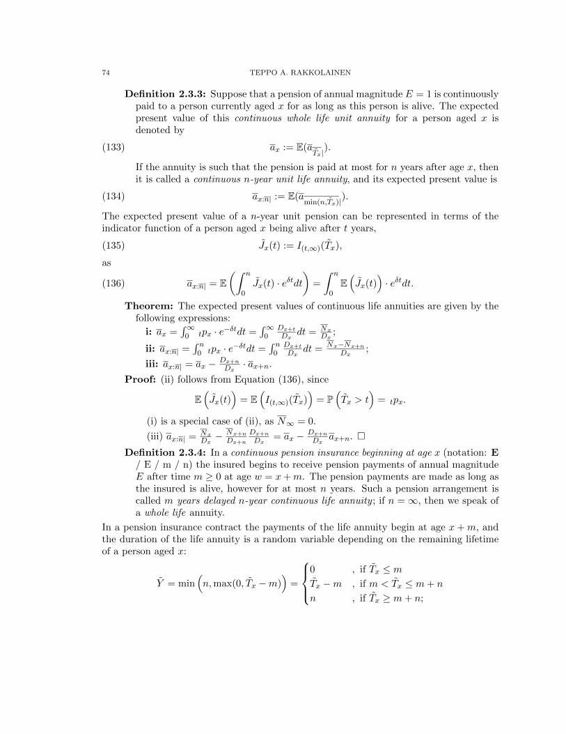
74 TEPPO A. RAKKOLAINEN
Definition 2.3.3: Suppose that a pension of annual magnitude E = 1 is continuouslypaid to a person currently aged x for as long as this person is alive. The expectedpresent value of this continuous whole life unit annuity for a person aged x isdenoted by
(133) ax := E(aTx|
).
If the annuity is such that the pension is paid at most for n years after age x, thenit is called a continuous n-year unit life annuity, and its expected present value is
(134) ax:n| := E(amin(n,Tx)|).
The expected present value of a n-year unit pension can be represented in terms of theindicator function of a person aged x being alive after t years,
(135) Jx(t) := I(t,∞)(Tx),
as
(136) ax:n| = E(∫ n
0Jx(t) · eδtdt
)=
∫ n
0E(Jx(t)
)· eδtdt.
Theorem: The expected present values of continuous life annuities are given by thefollowing expressions:
i: ax =∫∞
0 tpx · e−δtdt =∫∞
0Dx+tDx
dt = NxDx
;
ii: ax:n| =∫ n
0 tpx · e−δtdt =∫ n
0Dx+tDx
dt = Nx−Nx+n
Dx;
iii: ax:n| = ax − Dx+nDx· ax+n.
Proof: (ii) follows from Equation (136), since
E(Jx(t)
)= E
(I(t,∞)(Tx)
)= P
(Tx > t
)= tpx.
(i) is a special case of (ii), as N∞ = 0.
(iii) ax:n| =NxDx− Nx+n
Dx+n
Dx+nDx
= ax − Dx+nDx
ax+n.
Definition 2.3.4: In a continuous pension insurance beginning at age x (notation: E/ E / m / n) the insured begins to receive pension payments of annual magnitudeE after time m ≥ 0 at age w = x+m. The pension payments are made as long asthe insured is alive, however for at most n years. Such a pension arrangement iscalled m years delayed n-year continuous life annuity ; if n =∞, then we speak ofa whole life annuity.
In a pension insurance contract the payments of the life annuity begin at age x+m, andthe duration of the life annuity is a random variable depending on the remaining lifetimeof a person aged x:
Y = min(n,max(0, Tx −m)
)=
0 , if Tx ≤ mTx −m , if m < Tx ≤ m+ n
n , if Tx ≥ m+ n;
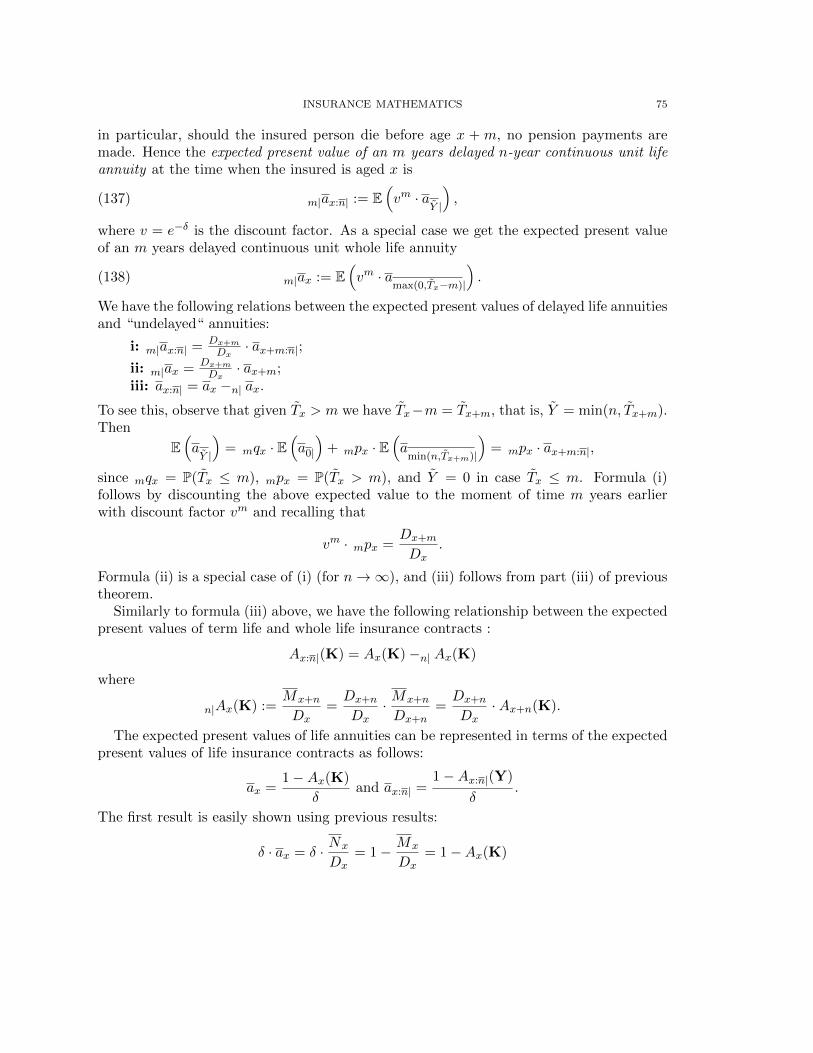
INSURANCE MATHEMATICS 75
in particular, should the insured person die before age x + m, no pension payments aremade. Hence the expected present value of an m years delayed n-year continuous unit lifeannuity at the time when the insured is aged x is
(137) m|ax:n| := E(vm · a
Y |
),
where v = e−δ is the discount factor. As a special case we get the expected present valueof an m years delayed continuous unit whole life annuity
(138) m|ax := E(vm · a
max(0,Tx−m)|
).
We have the following relations between the expected present values of delayed life annuitiesand “undelayed“ annuities:
i: m|ax:n| =Dx+mDx· ax+m:n|;
ii: m|ax = Dx+mDx· ax+m;
iii: ax:n| = ax −n| ax.
To see this, observe that given Tx > m we have Tx−m = Tx+m, that is, Y = min(n, Tx+m).Then
E(aY |
)= mqx · E
(a0|
)+ mpx · E
(a
min(n,Tx+m)|
)= mpx · ax+m:n|,
since mqx = P(Tx ≤ m), mpx = P(Tx > m), and Y = 0 in case Tx ≤ m. Formula (i)follows by discounting the above expected value to the moment of time m years earlierwith discount factor vm and recalling that
vm · mpx =Dx+m
Dx.
Formula (ii) is a special case of (i) (for n→∞), and (iii) follows from part (iii) of previoustheorem.
Similarly to formula (iii) above, we have the following relationship between the expectedpresent values of term life and whole life insurance contracts :
Ax:n|(K) = Ax(K)−n| Ax(K)
where
n|Ax(K) :=Mx+n
Dx=Dx+n
Dx· Mx+n
Dx+n=Dx+n
Dx·Ax+n(K).
The expected present values of life annuities can be represented in terms of the expectedpresent values of life insurance contracts as follows:
ax =1−Ax(K)
δand ax:n| =
1−Ax:n|(Y)
δ.
The first result is easily shown using previous results:
δ · ax = δ · Nx
Dx= 1− Mx
Dx= 1−Ax(K)
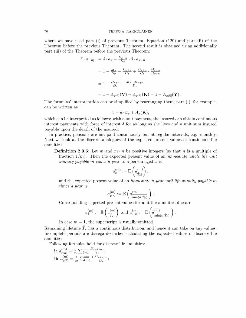
76 TEPPO A. RAKKOLAINEN
where we have used part (i) of previous Theorem, Equation (129) and part (ii) of theTheorem before the previous Theorem. The second result is obtained using additionallypart (iii) of the Theorem before the previous Theorem:
δ · ax:n| = δ · ax − Dx+nDx· δ · ax+n
= 1− MxDx− Dx+n
Dx+ Dx+n
Dx· Mx+n
Dx+n
= 1− Dx+nDx− Mx−Mx+n
Dx
= 1−Ax:n|(V)−Ax:n|(K) = 1−Ax:n|(Y).
The formulas’ interpretation can be simplified by rearranging them; part (i), for example,can be written as
1 = δ · ax +Ax(K),
which can be interpreted as follows: with a unit payment, the insured can obtain continuousinterest payments with force of interest δ for as long as she lives and a unit sum insuredpayable upon the death of the insured.
In practice, pensions are not paid continuously but at regular intervals, e.g. monthly.Next we look at the discrete analogues of the expected present values of continuous lifeannuities.
Definition 2.3.5: Let m and m · n be positive integers (so that n is a multiple offraction 1/m). Then the expected present value of an immediate whole life unitannuity payable m times a year to a person aged x is
a(m)x := E
(a
(m)
Tx|
),
and the expected present value of an immediate n-year unit life annuity payable mtimes a year is
a(m)x:n| := E
(a
(m)
min(n,Tx)|
).
Corresponding expected present values for unit life annuities due are
a(m)x := E
(a
(m)
Tx|
)and a
(m)x:n| := E
(a
(m)
min(n,Tx)|
).
In case m = 1, the superscript is usually omitted.
Remaining lifetime Tx has a continuous distribution, and hence it can take on any values.Incomplete periods are disregarded when calculating the expected values of discrete lifeannuities.
Following formulas hold for discrete life annuities:
i: a(m)x:n| =
1m
∑nmk=1
Dx+k/mDx
;
ii: a(m)x:n| =
1m
∑nm−1k=0
Dx+k/mDx
;
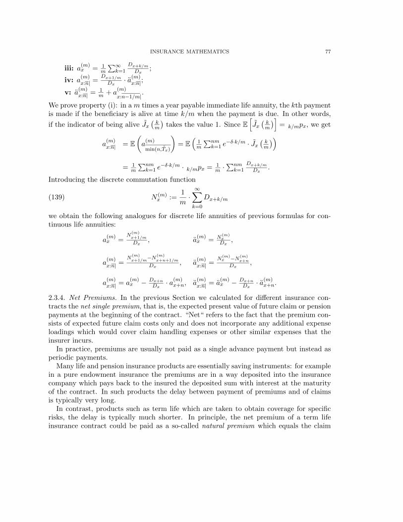
INSURANCE MATHEMATICS 77
iii: a(m)x = 1
m
∑∞k=1
Dx+k/mDx
;
iv: a(m)x:n| =
Dx+1/m
Dx· a(m)
x:n|;
v: a(m)x:n| =
1m + a
(m)
x:n−1/m|.
We prove property (i): in a m times a year payable immediate life annuity, the kth paymentis made if the beneficiary is alive at time k/m when the payment is due. In other words,
if the indicator of being alive Jx(km
)takes the value 1. Since E
[Jx(km
)]= k/mpx, we get
a(m)x:n| = E
(a
(m)
min(n,Tx)
)= E
(1m
∑nmk=1 e
−δ·k/m · Jx(km
))= 1
m
∑nmk=1 e
−δ·k/m · k/mpx = 1m ·∑nm
k=1Dx+k/mDx
.
Introducing the discrete commutation function
(139) N (m)x :=
1
m·∞∑k=0
Dx+k/m
we obtain the following analogues for discrete life annuities of previous formulas for con-tinuous life annuities:
a(m)x =
N(m)x+1/m
Dx, a
(m)x = N
(m)xDx
,
a(m)x:n| =
N(m)x+1/m
−N(m)x+n+1/m
Dx, a
(m)x:n| =
N(m)x −N(m)
x+n
Dx,
a(m)x:n| = a
(m)x − Dx+n
Dx· a(m)
x+n, a(m)x:n| = a
(m)x − Dx+n
Dx· a(m)
x+n.
2.3.4. Net Premiums. In the previous Section we calculated for different insurance con-tracts the net single premium, that is, the expected present value of future claim or pensionpayments at the beginning of the contract. “Net“ refers to the fact that the premium con-sists of expected future claim costs only and does not incorporate any additional expenseloadings which would cover claim handling expenses or other similar expenses that theinsurer incurs.
In practice, premiums are usually not paid as a single advance payment but instead asperiodic payments.
Many life and pension insurance products are essentially saving instruments: for examplein a pure endowment insurance the premiums are in a way deposited into the insurancecompany which pays back to the insured the deposited sum with interest at the maturityof the contract. In such products the delay between payment of premiums and of claimsis typically very long.
In contrast, products such as term life which are taken to obtain coverage for specificrisks, the delay is typically much shorter. In principle, the net premium of a term lifeinsurance contract could be paid as a so-called natural premium which equals the claim
78 TEPPO A. RAKKOLAINEN
intensity S · µt. In this case the premium for an infinitesimal time period [t, t+ dt] equalsthe expected value of claim costs for the time period, S ·µtdt. This premium changes withthe age of the insured and it is paid for as long as the insured is alive. Applied interest ratehas no effect on the premium, because (in expected value sense) there is no delay betweenpremiums and claim payments.
Definition 2.3.6: Let the age of the insured at the beginning of the contract be xand suppose that the premium is paid until age x+ h for as long as the insured isalive. Then h is the premium payment period of the insurance contract.
Continuous net level premium P is the constant continuous premium whose an-nual amount is P and which is paid during the premium payment period for as longas the insured is alive. Premium during time interval [t, t + dt] is Pdt, providedthat the insured is alive.
Discrete m times a year payable net premium due P (m) is paid during the pre-mium payment period for as long as the insured is alive in equally large installmentsperiodically so that period length is constant and total annual payment equals P (m).
There are many different methods to collecting premiums. In comparisons between alter-natives, the impact of interest needs to be taken into account.
Definition 2.3.7: Consider (possibly random) cash flows.i: Two cash flows (under the same interest rate assumptions) are equivalent, if
their expected present values are equal;ii: If two cash flows have different interest rate assumptions, their expected
present values can be equal at a specified moment of time t. Then thesecash flows are under the assumed interest rates equivalent at time t;
iii: Equivalence principle refers to adjusting (possibly random) cash flows to beequivalent (at a specified moment of time).
Assumed forces of interest need not be constants.
Equivalence principle is usually applied when setting premium levels in life or pensioninsurance to match the expected claim costs and other expenses.
In the following we assume that the insured is aged x at the beginning of the insurancecontract and that the premium payment period is h; additionally, force of interest δ isassumed to be constant.
The continuous level premium P equivalent to the net single premium A can be obtainedin accordance with equivalence principle from equation
(140) P · ax:h| = A.
In similar fashion, the discrete m times a year payable net premium due P (m) equivalent tothe net single premium A can be obtained in accordance with equivalence principle fromequation
(141) P (m) · a(m)
x:h| = A.
INSURANCE MATHEMATICS 79
Example: For a term life insurance (K/S/n) with premium payment period n, equa-tion (141) takes the form
P · ax:n| = S ·Ax:n|(K).
For a pension insurance (E/E/h/∞) with premium payment period h, equation(141) takes the form
P · ax:h| = E · h|ax.Example: Suppose that a person aged x enters into the following life insurance con-
tract: contract term is n, premium payment period is h and the contract consistsof a pure endowment insurance (V/S/n) complemented with a return-of-premiumpolicy such that in case the insured dies during the contract term, the paid premi-ums (without any interest) are paid to the beneficiary. In this case the continuouslevel premium can be solved from
P · ax:h| = S ·Ax:n|(V) + P · (IA)x:h|(K) + h · P · h|Ax:n−h|(K),
which yields
P =S ·Ax:n|(V)
ax:h| − (IA)x:h|(K)− h · h|Ax:n−h|(K),
where (IA)x:h|(K) is the expected present value of a linearly growing term life
contract in which the sum insured is t if the insured dies at age x + t with t ≤ h.This can be computed as
(IA)x:h|(K) :=∫ h
0 t · tpx · e−δt · µx+tdt
= 1Dx
∫ h0 t ·Dx+t · µx+tdt
= 1Dx·(−/h
0t ·Mx+t +
∫ h0 Mx+tdt
)= 1
Dx·(−h ·Mx+h +
∫ h0 Dx+tdt− δ ·
∫ h0 Nx+tdt
)= ax:h| −
(h · Mx+h
Dx+ δ
Dx
∫ h0 Nx+tdt
).
2.3.5. Multiple Life Insurance. An insurance contract can be dependent on the survival ordeath of more than one person, i.e. there may be several insured persons. This is calledmultiple life insurance or joint life insurance . Typical example is widow’s pension, wherethe widow is paid after the death of the spouse a pension for as long as the widow is alive.
Consider an insurance contract with two insured persons aged x and y. Their remaininglifetimes are Tx and Ty. The random variable
(142) Txy := min(Tx, Ty)
is the remaining lifetime until first death.
80 TEPPO A. RAKKOLAINEN
For simplicity, assume that lifetimes Tx and Ty are mutually independent, even thoughthis may not hold in practice (e.g. lifetimes of a married couple may not be independent).By virtue of independence,
tpxy := P(Txy > t) = P(Tx > t ∩ Ty > t
)= tpx · tpy = exp
(−∫ t
0 (µx+s + µy+s)ds),
and hence the joint mortality corresponding to remaining lifetime Txy is
(143) µxy+t = µx+t + µy+t.
This equation resembles the equations derived when dealing with competing causes ofdeath: in a sense, the insured persons’ collective (joint life status) dies as its first memberdies. Mathematically, joint life insurance contracts are similar to mortality models forseveral causes of death.
Example: In a unit widow’s pension (notation: (F/1)) the beneficiary Y is paid acontinuous unit pension (i.e. annual amount is E = 1) for as long as Y lives afterthe death of the insured person X. Let the ages of the insured and the beneficiary bex and y at initiation of the contract. To compute the expected present value of thiswidow’s pension, we use the indicators of being alive after time t has passed frominitiation of the contract, Jx(t) and Jy(t). Because the pension is paid when X isdead and Y is alive, the net single premium is (by virtue of assumed independenceof lifetimes)
E[∫∞
0 (1− Jx(t)) · Jy(t) · e−δtdt]
=∫∞
0 E[Jy(t)
]· e−δtdt−
∫∞0 E
[Jy(t)
]E[Jx(t)
]· e−δtdt
=∫∞
0 tpy · e−δtdt−∫∞
0 tpy · tpx · e−δtdt = ay − axy,
where axy :=∫∞
0 tpxy · e−δtdt is the expected present value of a continuous unit lifeannuity corresponding to joint mortality (143), in which pension is paid until thefirst death.
Of course, the net single premium could be deduced directly as follows: subtractfrom the expected present value of a unit whole life annuity paid to the (future)widow beginning from initiation of the contract the expected present value of aunit whole life annuity paid to the joint life status from initiation of the contract –the joint life status is “alive“for as long as both insured persons are alive, and thisis also the period from which the (future) widow does not yet receive pension.
Example: In a orphan’s pension (notation: (D/E/n)) the situation is similar towidow’s pension otherwise, but beneficiary Y is replaced by beneficiary Z aged z,to whom pension is paid after the death of the insured X at most until age w = z+n.The net single premium is
az:n| − axz:n|,where axz:n| :=
∫ n0 tpxz · e−δtdt. Observe that (F/E) = (D/E/∞).
INSURANCE MATHEMATICS 81
Calculations with multiple life statuses of more than two lives are in principle similar tothe two lives case.
Example: Three persons X, Y, and Z, aged x, y and z, enter the following insurancecontract: after the death of X, Y is paid a continuous annual pension of 1 and Zis paid a continuous annual pension of 0.2. If also Y dies, the continuous annualpension paid to Z rises to 0.6. Pension is paid to Y for whole remaining lifetimeand to Z at most until age w = z + n. Net single premium is
E[ ∫ n
0 1.2 · (1− Jx(t)) · Jy(t) · Jz(t) · e−δt+
+1.0 · (1− Jx(t)) · Jy(t) · (1− Jz(t)) · e−δt+
+0.6 · (1− Jx(t)) · (1− Jy(t)) · Jz(t) · e−δtdt+
+∫∞n (1− Jx(t)) · Jy(t) · e−δtdt
]=
= 1.2 ·∫ n
0 tqx · tpy · tpz · e−δtdt+ 1.0 ·∫ n
0 tqx · tpy · tqz · e−δtdt+
+0.6 ·∫ n
0 tqx · tqy · tpz · e−δtdt+ 1.0 ·∫∞n tqx · tpy · e−δtdt.
Inserting now tqh = 1− tph into the above formula yields
1.2 ·(ayz:n| − axyz:n|
)+ 1.0 ·
(ay:n| − axy:n| − ayz:n| + axyz:n|
)+
+0.6 ·(az:n| − axz:n| − ayz:n| + axyz:n|
)+ (ay − axy)−
(ay:n| − axy:n|
).
Combining terms gives
(ay − axy) + 0.6 ·(az:n| − axz:n|
)− 0.4 ·
(ayz:n| − axyz:n|
).
First term corresponds to widow’s pension to Y; the second and third terms cor-respond to such an orphan’s pension where we subtract from the orphan’s pension(D/0.6/n) an orphan’s pension paid to Z after X if Y is alive. If only X is deadbut Y is alive, then the pension paid to Z is (in annual amounts) 0.6− 0.4 = 0.2.
82 TEPPO A. RAKKOLAINEN
Consider an insurance contract involving k insured persons (X1, . . . , Xn), aged x := (x1, . . . , xk)at initiation of the contract (x is multiple joint life status). Denote
Tx := mini(Txi),
tpx := Πki=1 tpxi = P(Tx > t),
xpt := Πki=1 xipt,
µx+t·1 :=∑k
i=1 µxi+t,
Dx := xp0 · eδ·x, where x = 1k
∑ki=1 xi,
Nx :=∫∞
0 Dx+t·1dt,
Mx :=∫∞
0 Dx+t·1 · µx+t·1dt,
where 1 = (1, . . . , 1). Using these quantities, the formulas for single life annuities and insur-ance contracts generalize for multiple life annuities and insurance contracts. In particular,we have the following results (where annuities are paid until the first death).
i: ax =Nx
Dx;
ii: ax:n| =Nx−Nx+n·1
Dx;
iii: Ax:n|(K) =Mx−Mx+n·1
Dx= 1− δ · ax:n|.
Proof of (i)-(iii) is left as an exercise.
2.4. Technical Provisions. We have previously considered provisions. Provisions forinsurance liabilities are called technical provisions49 and form a very significant part ofan insurer’s balance sheet. By differentiation of the provision we can obtain a simpledifferential equation which facilitates deriving useful formulas for expected present valuesof insurance liabilities, different provisions and premiums.
Methods considered here are based on claim intensities, which are expected values. Hencethese methods do not allow us to consider the probability distributions of derived quantities.In this section we will not consider the corresponding stochastic differential equation, whichwould allow such considerations.
Technical provisions can be divided into two components: one related to claim eventsthat have already occurred and one related to claim events that will occur in the future.The first component is called outstanding claim provision50. This provision contains theexpected present values of all claim payments arising from claims that have occurred inthe past which have not yet been paid. In this course we will concentrate on the second
49technical provision = ansvarskuld = vastuuvelka50outstanding claim provision = ersattningsansvar = korvausvastuu
INSURANCE MATHEMATICS 83
component, the mathematical provision51, which contains the expected present values ofclaim payments from claim events that will occur in the future.
Mathematical provision can be calculated retrospectively, as the expected present valueof cumulative collected premiums less the expected present value of claim intensities. Ret-rospective provision (liability) is hence the result of premiums and claim payments notbeing simultaneous. Prospective provision, in contrast, is the expected present value of fu-ture claim payments less expected present value of future insurance premiums. Prospectiveprovision is hence the amount by which the expected present value of future claim costsexceeds the expected present value of future premiums.
It turns out that both calculation methods lead to same result, if the calculation basesfor premiums and provisions (claim intensities, interest rate assumptions and loadings) areidentical.
To shorten the notations, we adopt the following conventions:
Ax:w(·) := Ax:n|(·),
where w = x+ n is the termination age of the contract, and
Ax:w(·) = ax:w = 0, if x > w.
Correspondingly, we agree (in contrast to usual conventions in calculus) that the valueof an integral is zero if the lower bound of integration is larger that the upper bound ofintegration.
2.4.1. Prospective Provision. Prospective provision is the difference of the expected presentvalues of future claim costs and of future insurance premiums.
Expected present values of future claim costs for different insurance contracts were de-rived in previous sections. These net single premiums S ·Ax:w(·) are the expected presentvalues of future claim costs at the beginning of the contract when insured is aged x, andt years later the expected present value of future claim payments is S · Ax+t:w(·). Theexpected present value of future premiums P · ax:y has also been derived, and t years later
this value is P · ax+t:y (here y = x+m, where m is the premium payment term).
Definition 2.4.1: The prospective provision of an insurance contract during contractterm is
(144) Vt := S ·Ax+t:w(·)− P · ax+t:y.
Observe that for x+ t > y the second term is zero.
Example: Prospective provisions for term life insurance (K/S/n) and pure endow-ment insurance (V/S/n) can be expressed in terms of commutation functions asfollows:
Vt(K) = S · Mx+t −Mw
Dx+t− P · Nx+t −Ny
Dx+t
51mathematical provision = premieansvar = vakuutusmaksuvastuu
84 TEPPO A. RAKKOLAINEN
and
Vt(V) = S · Dw
Dx+t− P · Nx+t −Ny
Dx+t.
Example: Prospective provision for a pension insurance where the insurance is takenat age x and annual pension paid from age w = x+ n until age v equals E, can beexpressed in terms of commutation functions as follows:
Vt = E · Dw
Dx+t· aw:v − P ·
Nx+t −Ny
Dx+t.
2.4.2. Retrospective Provision. Retrospective provision is the difference of the expectedpresent values of paid premiums and of paid claim payments.
Expected present value of premiums paid until time t at the beginning of contract isP ·ax:t|, and accumulating this to time t we obtain the expected present value of premiumspaid until time t at time t as
P · ax:t| ·Dx
Dx+t.
The expected present value of past claim payments made until time t is S · Ax:t|(·), andhence their expected present value at time t is
S ·Ax:t|(·) ·Dx
Dx+t.
Definition 2.4.2: The retrospective provision of an insurance contract during pre-mium payment term (t ≤ y) is
(145) V retrot := P · ax:t| ·
Dx
Dx+t− S ·Ax:t|(·) ·
Dx
Dx+t;
after the premium payment term (t > y) the retrospective provision is
(146) V retrot := P · ax:ty| ·
Dx
Dx+t− S ·Ax:t|(·) ·
Dx
Dx+t,
i.e. only premium payment period is taken into account in the term related to paidpremiums.
Example: Retrospective provision for term life insurance (K/S/n) can be expressedin terms of commutation functions as follows:
V retrot (K) = P · Nx −Nx+t
Dx+t− S · Mx −Mx+t
Dx+t.
To establish the equality of retrospective and prospective provisions, we need the followingproposition:
Proposition: The following relations hold for life annuities and expected presentvalues of life insurance contracts:
i: ax:y = ax:t| +Dx+tDx· ax+t:y;
ii: Ax:w(K) = Ax:t|(K) + Dx+tDx·Ax+t:w(K);
INSURANCE MATHEMATICS 85
iii: Ax:w(V) = Dx+tDx·Ax+t:w(V) = Ax:x+t(V) ·Ax+t:w(V);
With the help of this proposition, it is possible to prove the following.
Theorem: Prospective provision equals retrospective provision for each insurancecontract type considered (i.e. term life K, pure endowment V and endowment lifeY), if the applied calculation base is the same.
Proofs of both this theorem and the preceding auxiliary proposition are left as exercises.
2.5. Thiele’s Differential Equation.
2.5.1. Basic Form of Thiele’s Equation. We shall next derive Thiele’s differential equationwith the formula for prospective provision (144) as our starting point. Multiplying equation(144) with Dx+t and differentiating with respect to t, we obtain Thiele’s equation
(147)d
dt(Vt ·Dx+t) = S · d
dt(Ax+t:w(K) ·Dx+t)− P ·
d
dt(ax+t:y ·Dx+t) .
Using previously proved representation results, we can compute more explicit expressionsfor the derivatives in equation (147):
ddt (Vt ·Dx+t) = V ′t ·Dx+t − (δ + µx+t) ·Dx+t · Vt;
ddt (Ax+t:w(K) ·Dx+t) = d
dt
(Mx+t −Mw
)= d
dt
(Mx+t
)= −µx+t ·Dx+t;
ddt (ax+t:y ·Dx+t) = d
dt
(Nx+t −Ny
)= d
dt
(Nx+t
)= −Dx+t
Inserting these expressions into equation (147) and dividing by Dx+t we obtain the basicform of Thiele’s differential equation
(148) V ′t − (δ + µx+t) · Vt = −S · µx+t + P .
Rearranging the terms yields
(149) V ′t = δ · Vt + µx+t · Vt + P − µx+t · S,
which gives us a decomposition of the growth V ′t of the provision into different components:the insurer earns interest (investment income) on the assets backing the provision, and fromthis interest the provision is credited with amount δ · Vt; the insurer receives premiums P ,which are added to the provision; upon death of the insured, the insurer pays the suminsured S, and the corresponding intensity µx+t · S is deducted from the provision; inaddition, upon the death of the insured the insurance terminates and the insurer’s liabilitiesdecrease by Vt, and hence the corresponding intensity µx+t · Vt is credited to the provision(so-called mortality bonus).
While the decomposition (149) was derived for term life insurance, it can be applied topure endowment and endowment life contracts by choosing the boundary conditions of thedifferential equation in a way consistent with the terms of the insurance contract type.
If a single premium P0 is paid at beginning of the contract term, then the initial conditionis set to V0 = P0; otherwise we set V0 = 0. Similarly, if it is agreed that a sum S will be
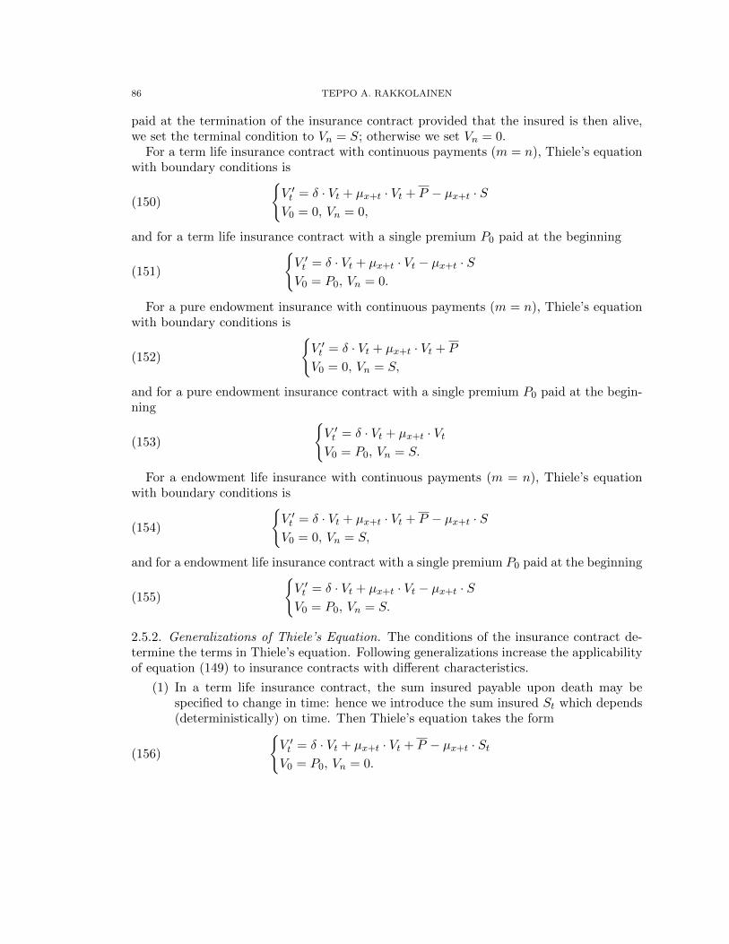
86 TEPPO A. RAKKOLAINEN
paid at the termination of the insurance contract provided that the insured is then alive,we set the terminal condition to Vn = S; otherwise we set Vn = 0.
For a term life insurance contract with continuous payments (m = n), Thiele’s equationwith boundary conditions is
(150)
V ′t = δ · Vt + µx+t · Vt + P − µx+t · SV0 = 0, Vn = 0,
and for a term life insurance contract with a single premium P0 paid at the beginning
(151)
V ′t = δ · Vt + µx+t · Vt − µx+t · SV0 = P0, Vn = 0.
For a pure endowment insurance with continuous payments (m = n), Thiele’s equationwith boundary conditions is
(152)
V ′t = δ · Vt + µx+t · Vt + P
V0 = 0, Vn = S,
and for a pure endowment insurance contract with a single premium P0 paid at the begin-ning
(153)
V ′t = δ · Vt + µx+t · VtV0 = P0, Vn = S.
For a endowment life insurance with continuous payments (m = n), Thiele’s equationwith boundary conditions is
(154)
V ′t = δ · Vt + µx+t · Vt + P − µx+t · SV0 = 0, Vn = S,
and for a endowment life insurance contract with a single premium P0 paid at the beginning
(155)
V ′t = δ · Vt + µx+t · Vt − µx+t · SV0 = P0, Vn = S.
2.5.2. Generalizations of Thiele’s Equation. The conditions of the insurance contract de-termine the terms in Thiele’s equation. Following generalizations increase the applicabilityof equation (149) to insurance contracts with different characteristics.
(1) In a term life insurance contract, the sum insured payable upon death may bespecified to change in time: hence we introduce the sum insured St which depends(deterministically) on time. Then Thiele’s equation takes the form
(156)
V ′t = δ · Vt + µx+t · Vt + P − µx+t · StV0 = P0, Vn = 0.
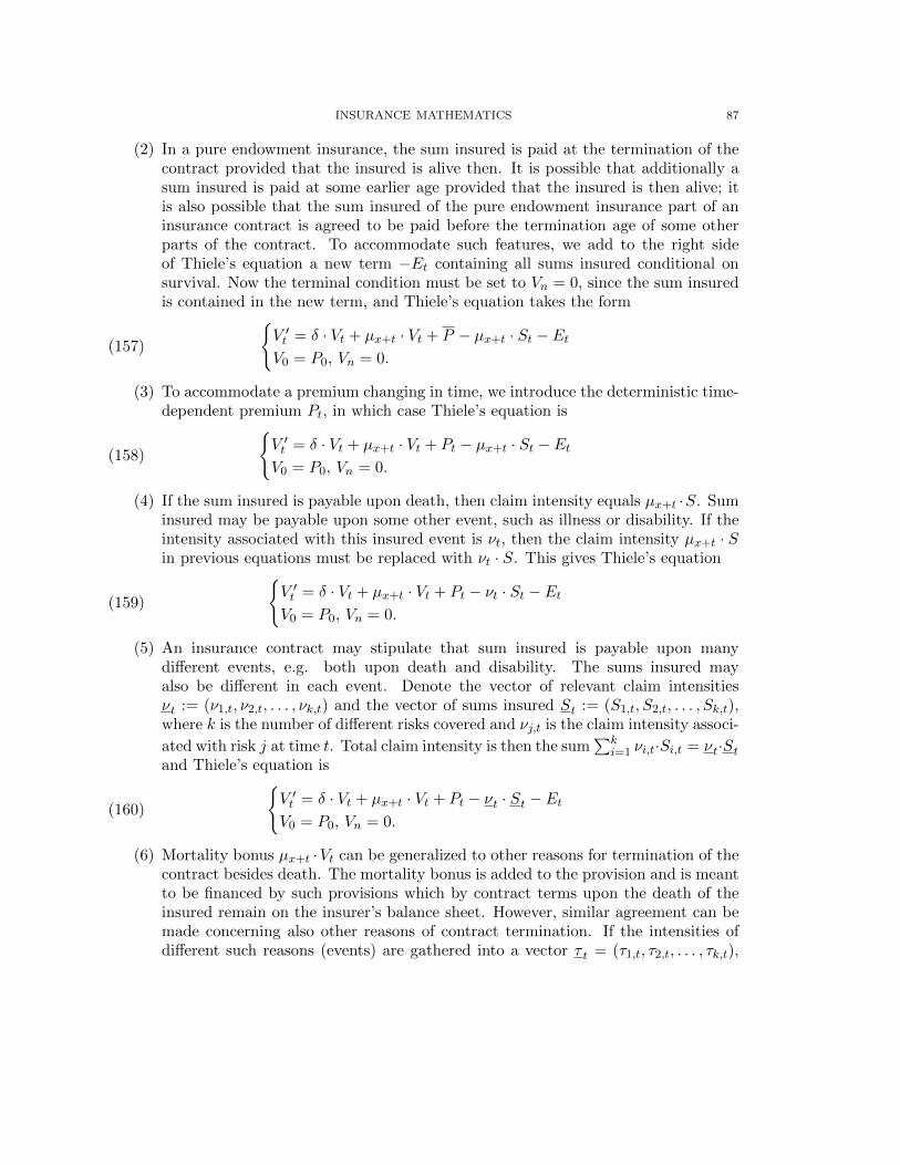
INSURANCE MATHEMATICS 87
(2) In a pure endowment insurance, the sum insured is paid at the termination of thecontract provided that the insured is alive then. It is possible that additionally asum insured is paid at some earlier age provided that the insured is then alive; itis also possible that the sum insured of the pure endowment insurance part of aninsurance contract is agreed to be paid before the termination age of some otherparts of the contract. To accommodate such features, we add to the right sideof Thiele’s equation a new term −Et containing all sums insured conditional onsurvival. Now the terminal condition must be set to Vn = 0, since the sum insuredis contained in the new term, and Thiele’s equation takes the form
(157)
V ′t = δ · Vt + µx+t · Vt + P − µx+t · St − EtV0 = P0, Vn = 0.
(3) To accommodate a premium changing in time, we introduce the deterministic time-dependent premium Pt, in which case Thiele’s equation is
(158)
V ′t = δ · Vt + µx+t · Vt + Pt − µx+t · St − EtV0 = P0, Vn = 0.
(4) If the sum insured is payable upon death, then claim intensity equals µx+t ·S. Suminsured may be payable upon some other event, such as illness or disability. If theintensity associated with this insured event is νt, then the claim intensity µx+t · Sin previous equations must be replaced with νt · S. This gives Thiele’s equation
(159)
V ′t = δ · Vt + µx+t · Vt + Pt − νt · St − EtV0 = P0, Vn = 0.
(5) An insurance contract may stipulate that sum insured is payable upon manydifferent events, e.g. both upon death and disability. The sums insured mayalso be different in each event. Denote the vector of relevant claim intensitiesνt := (ν1,t, ν2,t, . . . , νk,t) and the vector of sums insured St := (S1,t, S2,t, . . . , Sk,t),where k is the number of different risks covered and νj,t is the claim intensity associ-
ated with risk j at time t. Total claim intensity is then the sum∑k
i=1 νi,t·Si,t = νt·Stand Thiele’s equation is
(160)
V ′t = δ · Vt + µx+t · Vt + Pt − νt · St − EtV0 = P0, Vn = 0.
(6) Mortality bonus µx+t ·Vt can be generalized to other reasons for termination of thecontract besides death. The mortality bonus is added to the provision and is meantto be financed by such provisions which by contract terms upon the death of theinsured remain on the insurer’s balance sheet. However, similar agreement can bemade concerning also other reasons of contract termination. If the intensities ofdifferent such reasons (events) are gathered into a vector τ t = (τ1,t, τ2,t, . . . , τk,t),
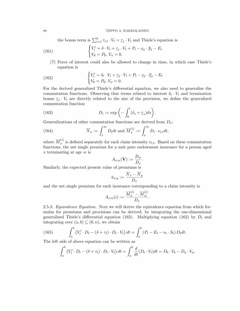
88 TEPPO A. RAKKOLAINEN
the bonus term is∑k
i=1 τi,t · Vt = τ t · Vt and Thiele’s equation is
(161)
V ′t = δ · Vt + τ t · Vt + Pt − νt · St − EtV0 = P0, Vn = 0.
(7) Force of interest could also be allowed to change in time, in which case Thiele’sequation is
(162)
V ′t = δt · Vt + τ t · Vt + Pt − νt · St − EtV0 = P0, Vn = 0.
For the derived generalized Thiele’s differential equation, we also need to generalize thecommutation functions. Observing that terms related to interest δt · Vt and terminationbonus τ t · Vt are directly related to the size of the provision, we define the generalizedcommutation function
(163) Dt := exp
(−∫ t
0(δs + τ s)ds
).
Generalizations of other commutation functions are derived from Dx:
(164) Nx :=
∫ ∞x
Dtdt and M(i)x :=
∫ ∞x
Dt · νi,tdt,
where M(i)x is defined separately for each claim intensity νi,t. Based on these commutation
functions, the net single premium for a unit pure endowment insurance for a person agedx terminating at age w is
Ax:w(V) :=Dw
Dx.
Similarly, the expected present value of premiums is
ax:y :=Nx −Ny
Dx
and the net single premium for each insurance corresponding to a claim intensity is
Ax:w(i) :=M
(i)x −M
(i)w
Dx.
2.5.3. Equivalence Equation. Next we will derive the equivalence equation from which for-mulas for premiums and provisions can be derived, by integrating the one-dimensionalgeneralized Thiele’s differential equation (162). Multiplying equation (162) by Dt andintegrating over (a, b) ⊆ (0, n), we obtain
(165)
∫ b
a
(V ′t ·Dt − (δ + τt) ·Dt · Vt
)dt =
∫ b
a(Pt − Et − νt · St)Dtdt.
The left side of above equation can be written as∫ b
a
(V ′t ·Dt − (δ + τt) ·Dt · Vt
)dt =
∫ b
a
d
dt(Dt · Vt)dt = Db · Vb −Da · Va,
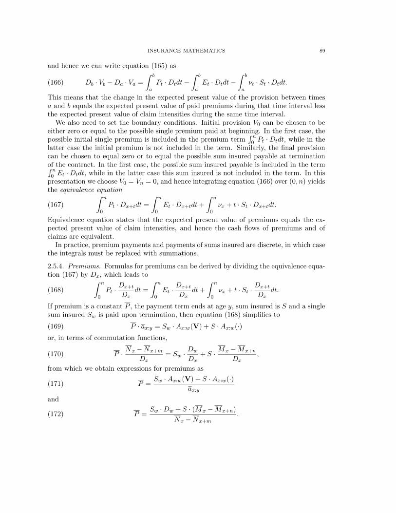
INSURANCE MATHEMATICS 89
and hence we can write equation (165) as
(166) Db · Vb −Da · Va =
∫ b
aPt ·Dtdt−
∫ b
aEt ·Dtdt−
∫ b
aνt · St ·Dtdt.
This means that the change in the expected present value of the provision between timesa and b equals the expected present value of paid premiums during that time interval lessthe expected present value of claim intensities during the same time interval.
We also need to set the boundary conditions. Initial provision V0 can be chosen to beeither zero or equal to the possible single premium paid at beginning. In the first case, thepossible initial single premium is included in the premium term
∫ n0 Pt ·Dtdt, while in the
latter case the initial premium is not included in the term. Similarly, the final provisioncan be chosen to equal zero or to equal the possible sum insured payable at terminationof the contract. In the first case, the possible sum insured payable is included in the term∫ n
0 Et ·Dtdt, while in the latter case this sum insured is not included in the term. In thispresentation we choose V0 = Vn = 0, and hence integrating equation (166) over (0, n) yieldsthe equivalence equation
(167)
∫ n
0Pt ·Dx+tdt =
∫ n
0Et ·Dx+tdt+
∫ n
0νx + t · St ·Dx+tdt.
Equivalence equation states that the expected present value of premiums equals the ex-pected present value of claim intensities, and hence the cash flows of premiums and ofclaims are equivalent.
In practice, premium payments and payments of sums insured are discrete, in which casethe integrals must be replaced with summations.
2.5.4. Premiums. Formulas for premiums can be derived by dividing the equivalence equa-tion (167) by Dx, which leads to
(168)
∫ n
0Pt ·
Dx+t
Dxdt =
∫ n
0Et ·
Dx+t
Dxdt+
∫ n
0νx + t · St ·
Dx+t
Dxdt.
If premium is a constant P , the payment term ends at age y, sum insured is S and a singlesum insured Sw is paid upon termination, then equation (168) simplifies to
(169) P · ax:y = Sw ·Ax:w(V) + S ·Ax:w(·)or, in terms of commutation functions,
(170) P · Nx −Nx+m
Dx= Sw ·
Dw
Dx+ S · Mx −Mx+n
Dx,
from which we obtain expressions for premiums as
(171) P =Sw ·Ax:w(V) + S ·Ax:w(·)
ax:y
and
(172) P =Sw ·Dw + S · (Mx −Mx+n)
Nx −Nx+m
.
90 TEPPO A. RAKKOLAINEN
2.5.5. Technical Provision. At initiation of the insurance contract, the insurer’s liabilityfor claims begins and the insurer begins to receive the agreed premiums. Future claimpayments are liabilities for the insurer and for accounting purposes are classified as insurer’sdebt to policyholders. This liability is called the technical provision, which the insurermust calculate annually. Previously derived formulas for provisions of term life, pureendowment and pension insurance contracts remain valid after generalizations made toThiele’s equation in section 2.5.2.
By integrating in equation (166) over (t, n) we obtain the equation for calculatingprospective provision
(173) Dn · Vn −Dt · Vt =
∫ n
tPt ·Dtdt−
∫ n
tEt ·Dtdt−
∫ n
tνt · St ·Dtdt.
Since the final provision Vn = 0, this can be solved for prospective provision Vt:
(174) Vt =
∫ n
tEu ·
Du
Dtdt−
∫ n
tνu · Su ·
Du
Dtdt−
∫ n
tPu ·
Du
Dtdt.
This could also be obtained directly from the one-dimensional Thiele’s differential equation(162) with final condition Vn = 0, using general solution formulas for non-homogeneousfirst order linear differential equations.
If premium is a constant P , the payment term ends at age y, sum insured is S and asingle sum insured Sw is paid upon termination, then the above equation is often written(when x+ t < y) as
(175) Vt = Sw ·Ax+t:w(V) + S ·Ax+t:w(·)− P · ax+t:y,
or, in terms of commutation functions, as
(176) Vt = Sw ·Dw
Dx+t+ S · Mx+t −Mw
Dx+t− P · Mx+t −Mw
Dx+t.
For x+ t ≥ y, the last term (premiums) vanishes.In similar fashion, by integrating in equation (166) over (0, t) we obtain the retrospective
provision
(177) V retrot =
∫ t
0Pu ·
Du
Dtdu−
∫ t
0Eu ·
Du
Dtdu−
∫ t
0Su · νu ·
Du
Dtdu,
and it has representations
V retrot = P · ax:x+t ·
Dx
Dx+t− S ·Ax:x+t ·
Dx
Dx+t= P · Nx −Nx+t
Dx+t− S · Mx −Mx+t
Dx+t.
If the calculation bases for premiums are the same, prospective and retrospective provisionsare equal also in the generalized case. Retrospective provision (177) could also be obtaineddirectly from the one-dimensional Thiele’s differential equation (162) with initial conditionV0 = 0, using general solution formulas for non-homogeneous first order linear differentialequations.
INSURANCE MATHEMATICS 91
Example: For a term life insurance with a constant premium, Thiele’s differentialequation is
V ′t = δ · Vt + µx+t · Vt + P − µx+t · S,with boundary conditions Vn = V0 = 0. Equivalence equation is∫ m
0P ·Dx+tdt =
∫ n
0S · µx+t ·Dx+tdt,
where Dx = exp(−∫ x
0 (δ + µs)ds). If payment term ends at age y, dividing by Dx
we obtain from above equation the form
P · ax:y =
∫ n
0S · µx+t ·
Dx+t
Dxdt.
Prospective provision at time t is during premium payment term
Vt = S ·Ax+t:w(K)− P · ax+t:y
(after premium payment term the last term is zero).
Example: For a pure endowment insurance, Thiele’s differential equation is
V ′t = δ · Vt + µx+t · Vt + Pt,
with boundary conditions V0 = 0, Vn = Sw. Equivalence equation is∫ m
0Pt ·Dx+tdt = Sw ·Dw,
where Dx = exp(−∫ x
0 (δ + µs)ds). If payment term ends at age y and payment is
constant Pt = P , dividing by Dx we obtain from above equation the form
P · ax:y = Sw ·Ax:w(V).
Prospective provision at time t is during premium payment term
Vt = Sw ·Ax+t:w(V)− P · ax+t:y
(after premium payment term the last term is zero).
Example: For a pension insurance, Thiele’s differential equation is
V ′t = δ · Vt + µx+t · Vt + Pt,
with boundary conditions V0 = 0, Vn = E · aw:w′ . Equivalence equation is∫ m
0Pt ·Dx+tdt = E · aw:w′ ·Dw,
where Dx = exp(−∫ x
0 (δ + µs)ds). If payment term ends at age y and payment is
constant Pt = P , dividing by Dx we obtain from above equation the form
P · ax:y = E · n|ax:w′−w|.
Prospective provision at time t is during premium payment term
Vt = E · aw:w′ ·Dw
Dx+t− P · ax+t:y
92 TEPPO A. RAKKOLAINEN
(after premium payment term the last term is zero).
Example: Consider an insurance contract where the insurer pays sum insured S ifthe contract terminates because of disability, death or attaining of the terminationage w. If the disability intensity for a person aged x+ t is νx+t, Thiele’s differentialequation is
V ′t = (δ + µx+t + νx+t) · Vt − (µx+t + νx+t) · S + Pt,
with boundary conditions V0 = 0, Vn = S. Equivalence equation is∫ m
0Pt ·Dx+tdt = S ·Dw + S ·
∫ n
0(µx+t + νx+t) ·Dx+tdt,
where Dx = exp(−∫ x
0 (δ + µs)ds). If payment term ends at age y and payment is
constant Pt = P , we obtain from above equation the form
P · ax:y = S ·Ax:w(V) + S ·Ax:w,
where Ax:w :=∫ n
0 (νx+t + µx+t) · DwDx+t
dt. Prospective provision at time t is during
premium payment term
Vt = S ·Ax+t:w(V) + S ·Ax+t:w − P · ax+t:y
(after premium payment term the last term is zero).
Example: Consider an insurance contract where the insurer pays sum insured Swhen first of the two insured persons dies (notation: KK). Now claim intensity forjoint life status is νt = µx+t + µy+t, and Thiele’s differential equation is
V ′t = (δ + µx+t + µy+t) · Vt − (µx+t + µy+t) · S + Pt,
with boundary conditions V0 = 0, Vn = 0. With constant continuous payment P ,equivalence equation is
P ·∫ m
0Dxy+tdt = S ·
∫ n
0(µx+t + µy+t) ·Dxy+tdt,
where Dxy+t = exp(−∫ t
0 (δ + µx+s + µy+s)ds)
. If payment term is m, we obtain
from above equation the form
P · axy:m| = S ·Axy:n|(KK),
where Axy:n|(KK) :=∫ n
0 (µx+t + µy+t) · Dxy+tDxydt. Prospective provision at time t is
during premium payment term
Vt = S ·Axy+t:n−t|(KK)− P · axy+t:m−t|
(after premium payment term the last term is zero).
INSURANCE MATHEMATICS 93
2.6. Expense Loadings. Previously derived premiums cover the insurer’s expected claimcosts. In addition to these costs, the insurer incurs operating or administrative expenses,such as wages and social security payments of employees. To cover these expenses, anexpense loading is added to the insurance premium. We denote net premiums (whichexclude expense loadings) by P and gross premiums which include expense loadings by B.
Loadings can be proportional, e.g.
i: proportional to gross premium, κ ·Bt;ii: proportional to sum insured, ε · St;iii: proportional to claim intensity, φ · νt · Stiv: proportional to provision, γ · Vt;
or absolute, such as
i: the expenses incurred when setting up the insurance contract;ii: constant annual expenses from administration of the contract and claim handling.
Equivalence principle is generalized to gross premiums as follows:
(178) PV of gross premiums = PV of claim costs + PV of expenses
As with claim costs, in this presentation present value of expenses is computed as anexpected value.
Thiele’s differential equation is now
(179) V ′t = (δ + τt) · Vt +Bt − Et − νt · St − Lt,where Lt is the expense loading at time t, which can contain both proportional and absoluteloadings (see list above). As before, integration over [a, b] ⊆ [0, n] yields
(180) DbVb −DaVa =
∫ b
aBt ·Dtdt−
∫ b
aEt ·Dtdt−
∫ b
aSt · νt ·Dtdt−
∫ b
aLt ·Dtdt.
One interpretation of this equation is that premiums increase technical provisions to theextent that they are not needed to cover claim costs and operating expenses.
Equivalence equation taking into account expense loadings is
(181)
∫ m
0Bt ·Dx+tdt =
∫ n
0Et ·Dx+tdt+
∫ n
0St · νx+t ·Dx+tdt+
∫ n
0Lt ·Dx+tdt.
For level continuous gross premium B and constant sums insured Sw and S we have
B · ax:y = Sw ·Ax:w(V) + S ·Ax:w(·) +
∫ n
0Lt ·
Dx+t
Dxdt,
from which we can solve the gross premium
B =Sw ·Ax:w(V) + S ·Ax:w(·) +
∫ n0 Lt · Dx+tDx
dt
ax:y.
Prospective provision takes the form
Vt =
∫ n
tEu ·
Du
Dtdu+
∫ n
tSu · νu ·
Du
Dtdu+
∫ n
tLu ·
Du
Dtdu−
∫ n
tBu ·
Du
Dtdu,
94 TEPPO A. RAKKOLAINEN
or (with constant level gross premium and constant sums insured)
Vt = Sw ·Ax+t:w(V) + S ·Ax+t:w +
∫ n
tLs ·
Dx+s
Dx+tds−B · ax+t:y,
i.e. prospective provision is the expected present value of future claim costs and expensesless the expected present value of future premiums.
Retrospective provision with expense loadings is
V retrot =
∫ t
0Bu ·
Du
Dtdu−
∫ t
0Eu ·
Du
Dtdu−
∫ t
0Su · νu ·
Du
Dtdu−
∫ t
0Lu ·
Du
Dtdu,
i.e. retrospective provision is the expected present value of past premiums less the expectedpresent value of past claim costs and expenses.
Example: Consider an Y-insurance, in which the insurer increases the premiumsto cover its operating expenses as follows: during premium payment term, amountκ·Bt is charged from contract and during contract term amounts ε·S and φ·µx+t ·Sare charged from contract. Hence the expense loading is
Lt = κ ·Bt + ε · S + φ · µx+t · S.
Thiele’s differential equation is
V ′t − (δ + µx+t) · Vt = Bt − µx+t · S − Lt = (1− κ) ·Bt − (1 + φ) · µx+t · S − ε · S
with boundary conditions V0 = 0 and Vn = S. From this we get for [a, b] ⊂ [0, n]
Vb ·Dx+b−Va ·Dx+a = (1−κ) ·∫ b
aBt ·Dx+tdt−S ·Dw−S ·
∫ b
a((1 + φ)µx+t + ε) ·Dx+tdt.
Equivalence equation is
(1− κ) ·∫ n
0Bt ·Dx+tdt = S ·Dw + S ·
∫ n
0((1 + φ)µx+t + ε) ·Dx+tdt,
and dividing by Dx and assuming Bt = B, we obtain equivalence
(1− κ) ·B · ax:y = S ·Ax:w(V) + S · ((1 + φ)Ax:w(K) + ε · ax:w) ,
gross premium
B =S ·Ax:w(V) + S · ((1 + φ)Ax:w(K) + ε · ax:w)
(1− κ) · ax:y
and prospective provision
Vt = S · (Ax+t:w(V) + (1 + φ)Ax+t:w(K) + ε · ax+t:w)− (1− κ) ·B · ax+t:y.
2.7. Some Special Issues in Life Insurance Contracts.
INSURANCE MATHEMATICS 95
2.7.1. Surrender Value and Zillmerization. Insurance contract may stipulate that the pol-icyholder has the right (option) to terminate the contract before the end of the contractterm. In this case the insured sells the contract back to the insurer and the insurer buysthe contract and pays its surrender value52 to the policyholder. Surrender value is at mostthe technical provision of the contract.
Since the insurer has paid as operating expenses the acquisition costs of the contract,policyholder’s exercise of the surrender option may cause losses to the insurer depending onhow the acquisition costs are amortized from expense loadings. In case an absolute initialloading equal to actual acquisition costs is used, no losses will arise. In practice, however,acquisition costs are often covered instead by increasing other loadings. Suppose that inorder to cover acquisition costs I, the loading proportional to gross premiums is increasedfrom κ to κ′ in such a way that
I = (κ′ − κ) ·B · ax:y.
The provision is for loadings (0, κ′)
S · ((1 + φ) ·Ax+t:w + ε · ax+t:w)− (1− κ′) ·B · ax+t:y.
If loadings (I, κ) had been used, the provision would be
S · ((1 + φ) ·Ax+t:w + ε · ax+t:w)− (1− κ) ·B · ax+t:y,
which is smaller by amount (κ′−κ)·B ·ax+t:y. The principle of reducing the surrender valuepaid to the policyholder by the amount of deferred acquisition costs is called zillmeringor zillmerization. In practice, this is taken into account approximatively by reducing fromthe provision amount
Z(t) = B · (κ′ − κ) · (m′ − t)+.
where m′ = min(m, 10). Often in practice contract-by-contract zillmering is not used whencalculating technical provisions for annual accounts; instead, an estimate of the sum ofindividual zillmerings is subtracted from the technical provisions.
The provision of the contract at time t, Vt, is called the non-forfeiture value53 of thecontract; the surrender value is Vt−Z(t), i.e. non-forfeiture value less individual zillmering.Technical provisions for annual accounts are calculated as the sum of non-forfeiture valuesless an estimate of the sum of zillmerings.
2.7.2. Changes in Contract after Initiation. In case changes are made in an insurancecontract after initiation, they are taken into account by applying the equivalence principle:i.e. surrender value or non-forfeiture value of the contract must remain invariant withrespect to the change. A change could be a modification of the insurance cover (e.g. suminsured is changed) or a discontinuation of premium payments.
In case insurance cover is modified but premium payments continue, equivalence principlerequires that non-forfeiture value must remain invariant. The equality of non-forfeiture
52surrender value = aterkopsvarde = takaisinostoarvo53non-forfeiture value = andringsvarde = muutosarvo
96 TEPPO A. RAKKOLAINEN
values V oldt = V new
t can be written as
Soldw ·Ax+t:w(V) + Sold · ((1 + φ) ·Ax+t:w + ε · ax+t:w)− (1− κ) ·Bold · ax+t:y =
= Sneww ·Ax+t:w(V) + Snew · ((1 + φ) ·Ax+t:w + ε · ax+t:w)− (1− κ) ·Bnew · ax+t:y.
If premium payments are discontinued, then the new premium level is 0 and equivalenceprinciple requires determining the level of insurance cover earned with paid premiums – thepaid-up value of the contract. Insurance cover may be adjusted either by reducing the suminsured or shortening the contract term. If sums insured are adjusted and the acquisitioncosts have already been amortized, then the paid-up value is
Vt = Sneww ·Ax+t:w(V) + Snew · ((1 + φ) ·Ax+t:w + ε · ax+t:w) .
In case deferred acquisition costs are not recoverable during remaining contract term, thenwe must use surrender value:
Vt − Z(t) = Sneww ·Ax+t:w(V) + Snew · ((1 + φ) ·Ax+t:w + ε · ax+t:w) .
2.7.3. Analysis and Surpluses. Since∫ ba V′t dt = Vb − Va, integrating Thiele’s equation over
[a, b] ⊂ [0, n] yieds
(182) Vb − Va =
∫ b
aδ · Vtdt+
∫ b
aτt · Vtdt+
∫ b
aBtdt−
∫ b
aEtdt−
∫ b
aνt · Stdt−
∫ b
aLtdt,
which states that the increase in insurer’s liabilities consists of interest credited to thepolicies, termination bonus and paid premiums less paid endowment claims, charges forcovering the claim costs arising from insured risks and loadings for covering insurer’s op-erating expenses.
Rearranging equation(183) gives
(183) Vb − Va −∫ b
aBtdt+
∫ b
aEtdt =
∫ b
aδ · Vtdt−
∫ b
a(νt · St − τt · Vt)dt−
∫ b
aLtdt.
On the right hand side are the assumptions on interest yield, claim costs and expenses usedin calculations. Insurers analyse annually how correct these assumptions have been on ag-gregate (summed over all contracts in the insurer’s portfolio). If the investment return fromthe insurer’s investment activity is larger than the assumed interest yield, the insurer hasduring the year accrued an interest rate surplus. Similarly, comparing the second term onthe right hand side to paid claim costs less provisions released from terminated contractsyields the insurer’s risk surplus, and deducting the year’s actual operating expenses fromloadings term yields the expense surplus. Usually there will be surpluses as the law re-quires the actuarial assumptions used for calculating premiums and provisions (first ordercalculation basis) to be determined prudently to ensure the survival of the insurer and thepolicyholders’ benefits. As the realized experience (second order basis) usually turns out tobe more advantageous to the insurer than what was assumed when setting premiums, theinsurer is on average expected to generate surpluses systematically. A reasonable amount
INSURANCE MATHEMATICS 97
of this surplus should be distributed back to policyholders as discretionary bonuses. Anal-ysis of different surpluses can be used to determine to which contracts bonuses are given(e.g. bonuses can be paid to contracts which have generated largest surpluses).
Integration over the whole contract term yields
(184)
∫ n
0δ · Vtdt+
∫ n
0τt · Vtdt+
∫ n
0Btdt =
∫ n
0Etdt+
∫ n
0νt · Stdt+
∫ n
0Ltdt,
which states that the insurer finances its costs from the contract (endowment payments,risk sums and expenses) with its proceeds (premiums, investment income and provisionsreleased due to termination of contract) from the contract.
Example: For an endowment life insurance the change in the technical provisionduring time interval (a, b) is
Vb− Va−∫ b
aBtdt = δ ·
∫ b
aVtdt−
∫ b
aµx+t · (S− Vt)dt−
∫ b
a(κ ·Bt + φ · µx+t · S + ε · S) dt.
Quantity S − Vt is called sum at risk at time t. Most often the time intervalconsidered is the past accounting year, i.e. [a, b] = [t− 1, t] and previous equationtakes the form
B +
∫ t
t−1δ · Vudu−∆Vt =
∫ t
t−1µx+u(S − Vu)du+
(κ ·Bt + φ · S ·
∫ t
t−1µx+udu+ ε · S
),
i.e. the sum of the insurer’s proceeds from risk coverage and expense loadings equalthe sum of premium income and technical interest less the increase in liabilities(provision). Considered over the whole contract term, we have∫ n
0Btdt+
∫ n
0δ · Vtdt = S +
∫ n
0µx+t(S − Vt)dt+
∫ n
0(κ ·Bt + φ · S · µx+t + ε · S) dt.
That is, if the realized investment returns, mortality and expenses are equal to theassumptions used in the first order basis, then premiums and investment incomeare just sufficient to cover claim costs and operating expenses.
98 TEPPO A. RAKKOLAINEN
3. Multiple State Models in Life Insurance
3.1. Transition Probabilities. We now consider insurance contracts in which the claimpayments are conditional on the insured being in a specified state, such as e.g. disabled,ill with a specified sickness or dead. For this purpose we assume that an insured personcan be in s disjoint (mutually exclusive) states, and may jump from one state to anotheras time passes.
Definition 3.1.1: Let S(t) be a right-continuous random variable depending on aget of the insured and taking values in 1, . . . , s. Denote by
A(y) := mint∣∣ S(u) = S(y) for all u ∈ [t, y]
,
the most recent age of arrival into the state in which the insured is at age y. Theprobability that an insured person aged y moves from state j to state i by age z iscalled the conditional transition probability and is denoted
(185) pij(z, y |x) := P(S(z) = i | S(y) = j, A(y) = x
),
for x ≤ y ≤ z. We can gather these transition probabilities into a matrix p(z, y) =(pij(z, y |x)) containing transition probabilities between all states from age y to agez.
Observe that the previous definition does not exclude the insured visiting other states thani and j in between ages y and z. In the matrix p(z, y), x depends on the initial state j, i.e.is different for different elements of the matrix and is therefore left out of the notation.
We will assume that transition probabilities are differentiable; in practice they maybe even discontinuous: if there is a minimum age limit w for old age pension, then thetransition probability from active state to pensioner state is zero at any age before age wand strictly positive at age w.
Age x is taken into account in order to be able to have the transition probabilitiesdependent on for how long the insured has been in state j. For example, the probabilityof a disabled person becoming fit to work again depends strongly on the duration of thedisability. On the other hand, we are assuming that transition probability does not dependon the history of the insured before arriving to state j. In principle this restriction can beovercome by expanding the state space: simply consider being disabled for the first timeas a separate state from being disabled for the second time.
3.2. Markov Chains.
Definition 3.2.1: The stochastic process S(t) introduced in the previous section isa Markov chain, if none of the transition probabilities pij depend on how long theinsured has been in state j. In this case,
(186) pij(z, y) := P(S(z) = i | S(y) = j
),
for y ≤ z.

INSURANCE MATHEMATICS 99
Many processes which are not Markov chains can in theory be transformed to Markovchains by decomposing state j into states indexed by (j, y − x). Since the time spent instate j, y − x, is a continuous variable, this leads to infinite (even uncountable) numberof states. In principle, this may be solved by discretization (e.g. taking into account onlyinteger part of y − x); however, often this leads to unpractically many states.
The transition from state j to state i may happen via some other state k, and thetransition probability is the sum of probabilities of all possible transition routes:
Proposition: Let y ≤ z and S be a Markov chain. For each u ∈ [y, z], the Chapman–Kolmogorov equations hold:
(187) pij(z, y) =
s∑k=1
pik(z, u) · pkj(u, y);
in matrix form
(188) p(z, y) = p(z, u)p(u, y).
Proof: Firstly,
pij(z, y) = P(S(z) = i
∣∣ S(y) = j)
=∑s
k=1 P(S(z) = i
∣∣ S(u) = k, S(y) = j)· P(S(u) = k
∣∣ S(y) = j).
Because S is a Markov chain
pij(z, y) =∑s
k=1 P(S(z) = i
∣∣ S(u) = k)· P(S(u) = k
∣∣ S(y) = j)
=∑s
k=1 pik(z, u) · pkj(u, y).
Definition 3.2.2: The right derivative of the transition probability
µij(y |x) := limz→y+
pij(z, y |x)− pij(y, y |x)
z − yis called the transition intensity from state j to state i. If i = j, it is sometimescalled staying intensity. For a Markov process, we leave out x and |. We denotethe matrix of transition intensities by µ(y). If matrix differentiation is definedelementwise, then
(189)d
dzp(z, y)
∣∣z=y
= µ(y).
In the following operator ddz refers to right derivative. Since 1 =
∑si=1 pij(z, y |xj), differ-
entiation of both sides with respect to z and setting z = y yields
(190)∑i 6=j
µij(y |xj) = −µjj(y |xj),
that is, the staying intensity of a state is the negative of the sum of transition intensitiesto other states.
100 TEPPO A. RAKKOLAINEN
For j 6= i, transition intensity is non-negative and
(191) µij(y |x) = limz→y+
pij(z, y |x)
z − y≥ 0,
since pij(y, y |x) = 0. Staying intensity is non-positive and
(192) µii(y |x) = limz→y+
pii(z, y |x)− 1
z − y≤ 0,
since pii(y, y |x) = 1.Force of mortality is also an intensity, but it was defined in a different way in our
previous considerations. However, the definitions are equivalent (i.e. force of mortality isa transition intensity in the sense of this section).
Theorem: Dying is a stochastic process, if we define S(t) = 1, if the person is alive
at time t, and S(t) = 2, if the person is dead at time t. This process is a Markovchain and
µ21(y) = µy,
where the left hand side follows the notation of this section and the right hand sidefollows the notation of previous sections.
Proof: The event of a person alive at age y dying by age z is a Markov process,because probability of death depends only on age z and the fact that the personis alive at age y. Obviously, no additional information is contained in knowing forhow long the person has been alive at age y. The transition probability from state1 to 2 is
p21(z, y) = z−yqy = 1− exp
(−∫ z−y
0µy+udu
),
and hence
µ21(y) =d
dzp21(z, y)
∣∣z=y
=
(µz−y+y exp
(−∫ z−y
0µy+udu
))z=y
= µy.
Intensity of staying alive is then −µy, by virtue of equation (190).
Theorem: Consider ages y and z, y ≤ z, when S(t) is a Markov chain and Ei is theset of states from which state i is accessible. Then
(193)d
dzpij(z, y) =
∑k∈Ei
µik(z) · pkj(z, y),
or in matrix form
(194)d
dzp(z, y) = µ(y)p(z, y).
Proof: Differentiate Chapman–Kolmogorov equations (187) with respect to z to get
d
dzpij(z, y) =
s∑k=1
d
dzpik(z, u) · pkj(u, y)
INSURANCE MATHEMATICS 101
and set then u = z to gets∑
k=1
d
dzpik(z, u) · pkj(u, y)
∣∣u=z
=s∑
k=1
µik(z) · pkj(z, y).
The theorem follows, since by definition transition intensities from states k 6∈ Ei(from which state i is non-accessible) to state i are zero.
If transition intensities are known, then the transition probabilities can be solved fromequation (194) – it is a set of s first order linear differential equations, for which thefollowing general results hold.
3.3. A Very Short Interlude on Linear Differential Equations.
Theorem: Let n be a positive integer and [a, b] ⊂ R. Consider a set of n linear firstorder differential equations
y′1(t) = c11(t)y1(t) + . . .+ c1n(t)yn(t) + f1(t)
. . . . . .
y′n(t) = cn1(t)yn(t) + . . .+ cnn(t)yn(t) + fn(t),
where functions cij are continuous and functions yi differentiable on [a, b]. Thiscan be written in matrix form as y′(t) = C(t) · y(t) + f(t), where C = (cij),y = (y1, . . . , yn) and f = (f1, . . . , fn). If the vector of initial values y(a) is known,then this is an initial value problem. If f = 0, then the equations are homogeneous.If det(C(a)) 6= 0, then the initial value problem has a unique non-zero solution on[a, b].
We do not prove this theorem here, as it is a basic result in the theory of differentialequations. A general solution formula in terms of matrix exponential exp(C) exists, butwriting out the solution componentwise leads to infinite series. In some special cases thesolution is expressible algebraically in terms of real-valued functions.
Theorem: Equation
(195) cn(t) · y(n)(t) + . . .+ c1(t) · y′(t) + c0(t) · y(t) = f(t)
is an nth order linear differential equation, where f and ci, i = 0, . . . , n, are con-tinuous functions. If the initial values y(a), y′(a), . . ., y(n)(a) are known, this is aninitial value problem. This initial value problem has exactly n linearly indepedentsolutions.
We do not prove this theorem here. The proof is based, among other things, on the factthat any nth order linear differential equation can be transformed into a set of first orderlinear differential equations. If the coefficient functions are constants, we have the followingresult.
Theorem: Consider an nth order linear homogeneous differential equation with con-stant coefficients
(196) cn · y(n)(t) + . . .+ c1 · y′(t) + c0 · y(t) = 0, t ∈ [a, b].
102 TEPPO A. RAKKOLAINEN
The characteristic equation of this differential equation is
(197) cn · rn + . . .+ c1 · r + c0 = 0,
the left hand side of which is an nth order polynomial in r and, as such, has nzeroes in the complex plane C, by the fundamental theorem of algebra. If thecharacteristic equation has n different roots ri ∈ C, i = 1, . . . , n, then all solutionsof equation (196) are of form
(198) y(t) = Cn · ernt + . . .+ C2 · er2t + C1 · er1t,
where coefficients Ci ∈ C are uniquely determined from the initial values of theinitial value problem. If the characteristic equation has a kth order root (2 ≤ k ≤ n)rj , then in the solution (198) the sum Cj · erjt + . . .+ Cj · erjt is replaced by
Cjerjt + Cj+1 · t1 · erjt + . . .+ Cj+k−1 · tk−1 · erjt.
Functions appearing in the differential equations encountered in applications considered inthis presentation do not always satisfy the continuity requirements of previous theorems.However, the functions are piecewise continuous with a finite number of discontinuitypoints, and the theorems may be applied piecewise to such subintervals of [a, b] over whichthe functions are continuous. That is, first solve the equation on the first subinterval withinitial value equal to the original initial value, then on the second subinterval with initialvalue equal to the final value of the preceding subinterval plus any possible additional termarising at the discontinuity point, and so on until the whole interval has been covered.
3.4. Evolution of the Collective of Policyholders. In this section we consider a closed(i.e. no new entrants are allowed) collective of policyholders, whose initial distribution tostates 1, . . . , s is known. We are interested in the distribution of policyholders to statesat some later date.
Definition 3.4.1: Denote by li(y) the number of policyholders aged y in state i, and
the s-vector of these numbers by l(y) := (li(y))si=1.
Theorem: Suppose that the transitions of a policyholder between states are de-scribed by a Markov chain, and that the transition probabilities pij are the samefor all policyholders. If the number of policyholders aged y is l(y), then the con-ditional expected value of the number of policyholders after time t, conditional onl(y) = l(y), is (in matrix form)
l(y + t) := p(y + t, y)l(y)
or
li(y + t) :=
s∑j=1
pij(y + t, y) · lj(y).
INSURANCE MATHEMATICS 103
Then the expected value of the number of policyholders aged y in state i changesin time according to
d
dtli(y + t) =
s∑j=1
∑k∈Ei
µik(y + t)pkj(y + t, y) · lj(y).
For t = 0, we get
d
dyli(y) =
s∑j=1
µij(y) · lj(y).
Proof: By definition of expected value
li(y + t) = E(li(y + t) | l(y)
)=
s∑j=1
pij(y + t, y) · lj(y).
Then
d
dtli(y + t) =
s∑j=1
d
dtpij(y + t, y) · lj(y) =
s∑j=1
∑k∈Ei
µik(y + t) · pkj(y + t, y) · lj(y).
Since pkj(y, y) is zero for k 6= j and one for k = j, the last formula follows.
3.5. Solutions for Transition Probabilities.
Definition 3.5.1: We denote by
B(y) := min(t | S(t) 6= S(y), t > y
)the age of departure from the state the policyholder is in at age y. Probability ofa transition in one step is
pij(z, y |x) = P(S(z) = i | S(u) = i, B(y) ≤ u ≤ z and A(y) = x
).
Probability of no transition is
pjj(z, y |x) = P(S(t) = j, t ∈ [x, z]
).
We can rewrite equation (193) as
(199)d
dzpij(z, y) = µii(z) · pij(z, y) +
∑k 6=i,k∈Ei
µik(z) · pkj(z, y),
which is a first order linear differential equation for functions pij and can be integrated toform (using multiplication with integrating factor exp
(−∫µii(u)du
))
(200)
pij(z, y) = pij(y, y)·exp
(∫ z
yµii(u)du
)+
∫ z
y
exp
(∫ z
uµii(v)dv
)·∑
k 6=i,k∈Ei
µik(u) · pkj(u, y)
du.
104 TEPPO A. RAKKOLAINEN
For i 6= j, we have pij(y, y) = 0, and hence in that case the above general formulasimplifies to
(201) pij(z, y) =
∫ z
y
exp
(∫ z
uµii(v)dv
)·∑
k 6=i,k∈Ei
µik(u) · pkj(u, y)
du,
which states that the probability of a policyholder who at age y is in state j to be in statei at age z is the sum of probabilities of a policyholder who at age y is in state j being instate k at age u, in which age the policyholder moves to state i where he/she stays untilage z with probability exp(
∫ zu µii(v)dv) < 1 (since µii < 0).
For i = j, we have pij(y, y) = 1, and hence in that case the above general formulasimplifies to(202)
pjj(z, y) = exp
(∫ z
yµjj(u)du
)+
∫ z
y
exp
(∫ z
uµjj(v)dv
)·∑
k 6=j,k∈Ei
µjk(u) · pkj(u, y)
du.
which states that the probability that a policyholder who at age y is in state j is also atage z in state j is equal to the sum of the probability that the policyholder stays in statej all the time from age y to age z and the probability that the policyholder visits otherstates k 6= j in between but returns to state j by age z.
Previous two transition formulas hold true only for Markov chains. The following result,in contrast, holds more generally.
Theorem: The probability of a policyholder staying in state j all the time from agey to age z, when he/she has been in state j since age x, is
(203) pjj(z, y |x) = exp
(∫ z
yµjj(u |x)du
)= Πk 6=j exp
(−∫ z
yµkj(u |x)du
).
The probability of a one-step transition from state j to state i is
(204)
pij(z, y |x) =∫ zy
(pii(z, u |u) · µij(u |x) · pjj(u, y |x)
)du
=∫ zy
(exp
(∫ zu µii(v |u)dv
)· µij(u |x) · exp
(∫ uy µjj(v |x)dv
))du.
Proof: For the first equation, observe that since there is no transition to other state,
(205)d
dzpjj(z, y |x) = µjj(z |x) · pjj(z, y |x).
(The reasoning goes as follows: the first equation we encountered in the proof of
Chapman–Kolmogorov equations (187) is true for a process S which is not neces-sarily a Markov chain, and since we are now dealing with a staying intensity, in
INSURANCE MATHEMATICS 105
that equation we now have i = j = k and the equation reduces to
pjj(z, y |x) =
= P(S(z) = j | S(u) = j, S(y) = j, A(y) = x
)· P(S(u) = j | S(y) = j, A(y) = x
);
but since now A(y) = A(u) as in both ages we have been uninterrupted in state jfrom age x, this can be written as
pjj(z, y |x) = P(S(z) = j | S(u) = j, A(u) = x
)· P(S(u) = j | S(y) = j, A(y) = x
)= pjj(z, u |x) · pjj(u, y |x);
differentiation with respect to z and setting then u = z yields the differential equa-tion (205).) Solution of this differential equation with initial condition pjj(y, y |x) =1 is the expression after first equality sign in the first equation of the theorem. Theexpression after second equality follows from the fact that staying intensity is thenegative of the sum of transition intensities.
If the transition can only occur from state j to state i, then for a Markov chain
pij(z, y) =
∫ z
y
(exp
(∫ z
uµii(v)dv
)· µij(u) · pij(u, y)
)du,
i.e. after being in state j at age y the policyholder moves at age u from state j tostate i where he/she stays until age z. If the policyholder has been in state j sinceage x, then according to preceding interpretation the formula takes the form
pij(z, y |x) =
∫ z
y
(exp
(∫ z
uµii(v |u)dv
)· µij(u |u) · pij(u, y |x)
)du,
and this is true even if we are not dealing with a Markov chain, by a similar argu-ment used in deriving the differential equation (205). Inserting into this equationthe expressions for pii(z, u |u) and pjj(u, y |x) from the first equation of the theoremwe obtain the second equation of the theorem.
Example: Consider a Markov chain with an infinite (but countable) number of statesk, 1, 2, 3, . . . such that transition intensities from state i to state i + 1 are νi,transition intensities from state i to state k are µi and all other transition intensitiesare zero. The model states could be interpreted as follows: k is“dead“, odd i’s are“active after being disabled for i − 1 times“ and even i is “disabled for (i − 1)’thtime“. Suppose that a policyholder is in state 1 at age x and denote
pj1(t) := P(S(x+ t) = j | S(x) = 1
),
and denote the mortality intensity of a policyholder in state i by µi(t) := µki(x+ t)and the transition intensity νi(t) := µi+1,i(x + t). Since there is no returning to
106 TEPPO A. RAKKOLAINEN
earlier states, µij = 0 for j > i. Then, by the results of this chapter,
d
dtp11(t) = −(µ1(t) + ν1(t)) · p11(t).
Integrating this equation with initial condition p11(0) = 1 yields
p11(t) = exp
(−∫ t
0(µ1(u) + ν1(u))du
).
Since the only states from which j is accessible are j−1 and j (i.e. Ej = j−1, j),d
dtpj1(t) = νj−1(t) · pj−1,1(t)− (µj(t) + νj(t)) · pj1(t),
for j = 2, 3, . . .. Taking into account initial condition pj(0) = 0 yields
pj1(t) =
∫ t
0exp
(−∫ t
u(µj(z) + νj(z))
)· νj−1(u) · pj−1,j(u)du.
From this probabilities of being in state j can be calculated recursively. Examplegeneralizes in a straightforward fashion to the case where transitions from state ito any state j > i occur with intensity νij .
3.6. An Example of a Disability Model. Consider a three-state disability insurancewith states a: “active“, i: “invalid“ and k: “dead“. Disability pension is paid while thepolicyholder is invalid. Transitions may occur from state a to states i or k and from state ito states a or k. From state k no transitions back to other states may occur. If we assumethat transitions only depend on the age of the policyholder (i.e. that we are dealing with aMarkov chain), then transition probabilities can be derived from corresponding intensities.If the policyholder is aged x at the beginning, then transition intensities at age x + t aredenoted
i: τ(t) := intensity of becoming invalid;ii: ν(t) := intensity of returning to active state;iii: µa(t) := mortality of an active person;iv: µi(t) := mortality of an invalid.
Let the number of policyholders aged x at time t = 0 be l(0) = la(0) + li(0), where la(0)is the number of active policyholders and li(0) is the number of invalid policyholders. Weobtain a set of linear differential equations
l′j(t) =∑s
µjs(t) · ls(t),
which now takes the form
(206)
l′a(t) = −(µa(t) + τ(t)) · la(t) + ν(t) · li(t)l′i(t) = −(µi(t) + ν(t)) · li(t) + τ(t) · la(t.)
The solution of this pair of equations is in general not expressible in terms of finite sums.However, as was stated in the section on linear differential equations, subject to someregularity conditions the pair of equations has a unique solution (important for the use of
INSURANCE MATHEMATICS 107
numerical solution methods to make sense). We will next derive the transition probabilities,expected present values of life annuities for disability pensions and the net premium fordisability pension assuming that the solution is known. After that, we look at under whichconditions the pair of equations is in practice solvable.
Proposition: Let all policyholders be in active state at time t = 0, i.e. la(0) > 0 andli(0) = lk(0) = 0. At time t
paa(x+ t, x) = P(S(x+ t) = a | S(x) = a
)= la(t)
la(0)
pia(x+ t, x) = P(S(x+ t) = i | S(x) = a
)= li(t)
la(0)
pka(x+ t, x) = lk(t)la(0) = 1− paa(x+ t, x)− pia(x+ t, x).
(207)
Proof: Formula l·(y + t) =∑s
j=1 p·,j(y + t, y) · lj(y) reduces in this case to la(t) =
paa(x + t, x) · la(0), since li(0) = lk(0) = 0. This proves the first equation. Thesecond one is proved similarly, and the third follows from the preceding two.
Proposition: The policyholder has obtained insurance while in active state at age x.The insurer has agreed to pay a continuous unit disability pension for the durationof disability at most until age w = x + n. Premiums are paid continuously whilethe policyholder is in active state, however at most for m years. Force of interestis δ.
i: The expected present value of the future disability pension for a policyholderactive at age x+ t is
(208) aiax+t:w :=
∫ n
tpia(x+ u, x+ t) · e−δ(u−t)du.
ii: The expected present value of the sum of ongoing and future disability pen-sions for a policyholder invalid at age x+ t is
(209) aiix+t:w :=
∫ n
tpii(x+ u, x+ t) · e−δ(u−t)du.
iii: The expected present value of the ongoing disability pension for a policy-holder invalid at age x+ t is
(210) aix+t:w :=
∫ n
tpii(x+u, x+t)·e−δ(u−t)du =
∫ n
texp
(−∫ u
t(δ + µi(s) + ν(s))ds
)du.
iv: The continuous level insurance premium is
(211) P = E ·aiax:n|
aaax:m|,
108 TEPPO A. RAKKOLAINEN
where E is the annual amount of disability pension and
aaax:m| =
∫ m
0paa(x+ u, x+ t)e−δ·udu
is a life annuity payable while in active state.
Proof: Denote the indicator of being invalid by Jx+t(u) := Ii(S(x+ u)), where Ii isthe indicator of state i (invalid). Then the expected value of the random presentvalue of a continuous n-year unit pension is
aiax+t:w = E[∫ n
tJx+t(u) · e−δ(u−t)du
]=
∫ n
tE[Jx+t(u)
]· e−δ(u−t)du.
Part (i) of the proposition follows immediately, since
E[Jx+t(u)
]= E
[Ii(S(x+ u))
]= P
(S(x+ u) = i | S(x+ t) = a
)= pia(x+ u, x+ t).
Parts (ii) and (iii) are proved in completely similar fashion; for the second equal-ity in (iii), equation (203) is used. Part (iv) follows from equivalence principle.
The insurer’s technical provision for an invalid policyholder is the sum of expected presentvalues of ongoing and future disability pensions. The expected present value of ongoingdisability pension is a part of the outstanding claim provision, while the expected presentvalue of future disability pensions is a part of mathematical provision.
We conclude this example by considering how to solve the number of policyholders indifferent states at time t (i.e. equations (206)). As previously stated, in general a numericalsolution method is called for. However, if all the transition intensities are constants, a closedform analytical solution can be obtained. In this case, differentiating the first equation in(206) yields
l′′a(t) = −(µa + τ) · l′a(t) + ν · l′i(t).Inserting into this equation the expression for derivative l′i from the second equation of(206) yields
l′′a(t) = −(µa + τ) · l′a(t) + ν · [−(µi + ν) · li(t) + τ · la(t)]
= −(µa + τ) · l′a(t)− ν · li(t) · (µi + ν) + ν · τ · la(t)
Inserting into this an expression for ν · li(t) solved from the first equation of (206) yields asecond order linear homogeneous differential equation with constant coefficients
(212) l′′a +A · l′a +B · la = 0,
where A = τ + ν + µa + µi and B = (µa + τ) · (µi + ν) − τ · ν. This is solvable using thecharacteristic equation r2 +A · r +B = 0. The general solution is
la(t) = C1 · er1t + C2 · er2t,

INSURANCE MATHEMATICS 109
where r1 and r2 are the two different roots of the characteristic equation. Inserting la(t)into the second equation of (206) yields a first order differential equation for li(t), whichcan be solved to yield
li(t) = exp
(−∫ t
0(µi + ν)du
)·(li(0) +
∫ t
0τ · (C1 · er1u + C2 · er2u) · exp
(∫ u
0(µi + ν)ds
)du
).
For disability pensions, constant transition intensities are not really compatible with reality.Another assumption leading to closed form solution in this example is assuming that µi(t) =µa(t) =: µ(t), i.e. that the mortalities of active and disabled policyholders are the same.This is also typically not quite realistic, as most often the mortality of invalids is higher.
110 TEPPO A. RAKKOLAINEN
4. On Asset–Liability Management
Asset–Liability Management (ALM) refers to a holistic, total balance sheet approach inmanaging an insurer’s assets and liabilities as a whole. This means integrating the workof actuarial department focusing on the measurement, analysis and projection of insurer’sliabilities and their risks and the work of investment department focusing on the risksand rewards of asset classes and asset strategies. In particular, ALM is about recognizingthe importance of investment activities being in accordance with requirements set by thenature of the liabilities. One way of looking at ALM is to consider it as an optimizationproblem where our goal is to maximize financial returns subject to the constraint that wemust be able to cover our liabilities (with sufficiently high probability).
Classical concepts related to ALM are matching and immunization. Matching of assetswith liabilities involves in its purest form structuring the flow of asset proceeds to coincideexactly with the outgo with respect to liabilities. Doing this perfectly is of course possibleonly in a deterministic world where no uncertainty is associated with future cash flows.Depending on the nature of the liability, a close matching, however, may be possible –some life insurance products such as guaranteed income bonds can be closely matchedwith investments made in government fixed income securities. In contrast, matching assetsmay be exceedingly hard to find for e.g. some non-life insurance products. Immunization(first proposed by Redington in 1952) generalizes the concept of matching by requiringinvesting in such a way that a change in the value of assets is exactly matched by a changein the value of liabilities, i.e. that liabilities are immunized with respect to changes in valuedue to changes in some underlying factors (in Redington’s model, interest rates).
4.1. Classical Asset-Liability Theory. Suppose that insurer’s expected net liabilitiesat time t are given by Lt, and that the insurer’s expected asset proceeds payable at timet are given by At. Then with a force of interest δ, the present value of expected futureliabilities is
L(δ) :=
∫ ∞0
Lze−δzdz
and the present value of expected future asset proceeds is
A(δ) :=
∫ ∞0
Aze−δzdz.
Suppose now that assets and liabilities are initially matched under interest rate assumptionδ so that A(δ) = L(δ), and the interest changes from δ to δ + ε. Both L and A will nowchange, and by Taylor approximation
L(δ + ε) ≈ L(δ) + ε · L′(δ) +ε2
2· L′′(δ)
and
A(δ + ε) ≈ A(δ) + ε ·A′(δ) +ε2
2·A′′(δ).
INSURANCE MATHEMATICS 111
Hence
A(δ + ε)− L(δ + ε) ≈ A(δ)− L(δ) + ε ·(A′(δ)− L′(δ)
)+ε2
2·(A′′(δ)− L′′(δ)
).
The first term of the right hand side of above equation is zero since assets and liabilities wereinitially matched. If the change in interest rate should cause no profit or loss, then obviouslyall successive derivatives should be equal to zero. For small changes the first derivative isthe most important, and a portfolio with A′(δ)−L′(δ) = 0 is called an immunized portfolio.If furthermore A′′(δ) − L′′(δ) ≥ 0, then any sufficiently small change in interest rate willresult in a profit. Based on these observations, a satisfactory immunization strategy canbe characterized by A′(δ)− L′(δ) = 0 and A′′(δ)− L′′(δ) ≥ 0.
While this seems to make things very simple, it should be observed that in practice:the previous two equations have usually an infinite number of solutions; the equationsdefine the position at a moment in time – their solutions change continuously; solution isdependent on the interest rate (which is what interest rate, exactly?); the solution is basedon an approximation argument valid for small changes only; ...and many more problemsand complications can be found.
4.2. Immunization of Liabilities with Bonds. A very natural idea is to use default-freebonds (whose price or value is a function of interest rates) to construct an immunizationstrategy against interest rate changes. We will consider three strategies: multi-periodimmunization, generalized immunization and cash flow matching.
We need to be able to compute the yield and duration of a bond portfolio; while inprinciple this can be done by considering the portfolio as a single bond and solving theyield as we did for single bonds, in practice this is thought to be too cumbersome andapproximations are used. The yield of a bond portfolio is approximated by the presentvalue weighted average of individual bond yields
yp ≈∑N
k=1 Pkyk∑Nk=1 Pk
,
and similarly the bond portfolio’s duration is approximated by the present value weightedaverage of individual bond durations
Dp ≈∑N
k=1 PkDk∑Nk=1 Pk
.
When immunizing liabilities, we will employ a generalization of (Macaulay) duration, so-called ith generalized duration which is defined for an individual bond k as
DiGen:k :=
√W ik,
where
W ik :=
1
Pk
n−1∑t=0
((τ + t/m)iCFτ+t/m
(1 + yk)τ+t/m
112 TEPPO A. RAKKOLAINEN
(observe that D1Gen:k = DMac:k). The generalized duration of a bond portfolio is approxi-
mated by
DiGen:p ≈
∑Nk=1 PkD
iGen:k∑N
k=1 Pk.
Consider now an insurance product in which the insurer has promised a guaranteed rateof return to premium, i.e. the policyholder or beneficiaries receive a specified guaranteedpayment at a specified future date. We assume that the insurer invests in a single bond(using previous approximations the considerations generalize to a bond portfolio). Let hdenote the investment horizon and n1 the number of coupons that will be paid duringinvestment horizon. The value of the reinvested coupons on the horizon date (at time h) is
I =
n1−1∑t=0
CFτ+t/m · (1 + y)h−τ−t/m,
and the present value of the bond at horizon date is
H =
n−1∑t=n1
CFτ+t/m
(1 + y)τ+t/m−h .
The final wealth at the horizon date is W = I +H, and an increase in yield will result in ahigher I value and a lower H value. The derivative of the final wealth at the horizon datewith respect to the yield is
∂W∂y = ∂
∂y
[∑n1−1t=0 CFτ+t/m · (1 + y)h−τ−t/m +
∑n−1t=n1
CFτ+t/m(1+y)τ+t/m−h
]= h
(1+y)1−h
(∑n1−1t=0
CFτ+t/m(1+y)τ+t/m
+∑n−1
t=n1
CFτ+t/m(1+y)τ+t/m
)−
− 1(1+y)1−h
(∑n1−1t=0
(τ+t/m)CFτ+t/m(1+y)τ+t/m
+∑n−1
t=n1
(τ+t/m)CFτ+t/m(1+y)τ+t/m
)= P · (1 + y)h−1 · (h−DMac)
This implies that if
h−DMac
< 0 ⇒ ∂W
∂y < 0 ⇒ market risk
= 0 ⇒ ∂W∂y = 0 ⇒ immunized ALM portfolio
> 0 ⇒ ∂W∂y > 0 ⇒ reinvestment risk
Observe that previous analysis is based on a parallel shift of the yield curve. To summarize,for a bond portfolio a fall in interest rates will cause the portfolio to increase in value butthe coupons will be reinvested at a lower rate, while a hike in interest rates will causethe portfolio to decrease in value but the coupons will be reinvested at a higher rate. Atportfolio’s Macaulay duration the two opposite effects will approximately offset each other.To immunize a single liability against yield changes we need to choose a bond portfoliosuch that
INSURANCE MATHEMATICS 113
(1) Macaulay duration is equal to the investment horizon;(2) initial present value of the cash flows equals the present value of future liability.
However, immunization is only achieved if yield changes are parallel; moreover, as yieldchanges, the duration changes too. Continued immunization hence requires rebalancing theportfolio as time passes, and even then immunization is with respect to parallel changes inthe yield curve only.
Obviously a large number of portfolios fulfill the immunization requirements above.However, the more dispersion the cash flow of the portfolio has, the more immunizationrisk it has. The dispersion of the cash flow of the bond portfolio with respect to theinvestment horizon h can be measured with∑n−1
t=0 (τ + t/m− h)2 CFτ+t/m(1+y)τ+t/m∑n−1
t=0CFτ+t/m
(1+y)τ+t/m
.
Hence we might choose the immunized portfolio with the smallest dispersion among thepossible alternatives.
In reality, we usually have multi-period liabilities. In this case we can decompose theliabilities to single period liabilities each of which is immunized by a subportfolio of bonds.A multi-period immunization strategy must satisfy the following conditions:
(1) the Macaulay duration of the total bond portfolio must equal the duration of theportfolio of liabilities;
(2) the Macaulay duration distribution of the bond subportfolios must have a widerrange than the duration distribution of the liabilities;
(3) the present value of the cash flow from a subportfolio must equal the present valueof the corresponding liability stream; and
(4) for each liability the chosen subportfolio has the smallest dispersion among availablealternatives.
In generalized immunization, the bond portfolio is chosen in such a way that its general-ized durations up to some order match (immunize) the generalized durations of the liabilitystream. In practical applications the order is rarely higher than 1, which corresponds tousual immunization (matching of Macaulay durations).
In cash flow matching, the last (in time) individual liability cash flow is matched byinvestment in a bond with maturity equal to the time at which the liability is due andprincipal equal to the nominal value of the liability. After this, the remaining liability cashflows are reduced by the amount of coupon payments that will be received from the firstbond, and then the next to last liability is matched similarly with a bond. The processcontinues until all liabilities are matched. Observe that a perfectly cash flow matched port-folio is necessarily duration matched, but there may be many duration matched portfolioswhich are not cash flow matched. The benefits of this approach are that there is no needto compute any durations, no rebalancing is needed and there is no risk that the liabilitiescannot be satisfied (unless a bond issuer defaults). The downside of cash flow matchingis its high cost: finding matching bonds can be burdensome and still the matching cannot
114 TEPPO A. RAKKOLAINEN
usually be perfect, so that more capital than necessary will need to be set aside to matchthe liabilities – this may be inefficient capital management, because instruments used formatching are typically low risk and low return bonds and the insurer is not able to takeadvantage of high return investment opportunities. Naturally, one way of looking at thisis that the purpose of a matching portfolio is first and foremost to match the liabilities,while the free reserves (i.e. excess of assets over and above the liabilities) can be used togenerate high returns. An investment approach called core–satellite is related to this idea:the core portfolio attempts to hedge or replicate the liabilities, while the satellite portfoliosconcentrate on achieving high returns.
4.3. Stochastic Asset–Liability Management. ALM is concerned with risks and re-wards of investment strategies and insurance liabilities as a whole. First models of thistype were static, single-period models where a closed form solution was often obtainable.However, to take properly into account the complex time-dependent interrelationships anddependencies of assets and liabilities, and the impact of future management actions, a dy-namic approach using stochastic simulations is called for. Sufficiently realistic models willalmost invariably be too complex to be analytically solvable in closed form. However, theycan be used to simulate the development of assets and liabilities. The huge advances incomputing power have made this a more and more practical solution.
Competitive pressures have added complexity to the products offered by insurance com-panies: many contracts have implicit or explicit guarantees and embedded options, whichare difficult or impossible to evaluate otherwise than by simulations. Even if the risksare theoretically hedgeable, the hedging may in practice be very costly or impossible toimplement and the insurer may be willing or forced to leave part of the risk unhedged.Typical questions of interest are
i: What future economic conditions might lead to problems (losses) and how signifi-cant is the impact of the risk if realized?
ii: Are the asset allocation, business strategy and bonus policy appropriate? Whatactions could be taken to mitigate the risks?
iii: How much capital is required to support the mismatch of assets and liabilitiesand what is the trade-off between risk and return of this capital?
Future developments may be described by different economic scenarios. The cash flowsof a contract can then be evaluated under different scenarios to obtain an understandingof how the value of the contract is impacted by different future developments. To achievethis, historical or deterministic pre-specified scenarios can also be used, which reduces thecomputational effort; however, using a large number of stochastically simulated scenarioshas the advantage of giving a more complete picture of the future possibilities, includingthe impact of rare events and dependencies which may not have historical precedentsin available data and also may not be easily covered by a set of deterministic scenariosconstructed based on expert judgment (it is easy to overlook some less obvious possibilities).Of course, this requires that the stochastic dynamics are appropriately specified; however,despite this being a non-trivial task, building scenario-generating stochastic models withreasonably realistic assumptions is likely to provide a more complete picture of risks and
INSURANCE MATHEMATICS 115
rewards of assets and liabilities which include complex insurance products and financialinstruments than just relying on a few deterministic scenarios.
In an ALM model a special module often called Economic Scenario Generator (ESG)usually generates the scenarios for economic variables. Based on input from actuarialdepartment and from investment department, assets and liabilities are projected througheach scenario to obtain a range of possible outcomes. Simulation results can then beanalyzed with a view to the objectives of risk and reward. Especially with longer planninghorizons, it is important to incorporate future management actions and insurer’s businessand investment strategy into modeling. The longer the horizon, the more untenable isan assumption of a fixed investment strategy. An investor will react to changes in theeconomic environment and this should be reflected in a long term modeling of assets andliabilities.
Broadly speaking, the purpose of stochastic asset simulation can be prediction, pricingor risk analysis. Prediction is usually very short-term, as markets adapt to changingconditions and prediction of market movements on longer term is quite difficult. Pricingapplications often employ absence of arbitrage conditions to check that prices are consistentwith the prices of traded securities. Risk analysis evaluates the potential rewards and risksof various investment and liability management strategies, to facilitate avoiding undesired(unsustainable) risks and accepting some other risks to create opportunities for enhancedreturns.
Common stochastic asset modeling approaches in insurance are
i: mean–covariance approach, which relies on specifying expected values, variancesand covariances of assets – obviously, this approach traditionally relies on normalor lognormal time-independent distribution assumptions and hence is often lackingin realism;
ii: autoregressive approach with a cascade structure, where variables have hierarchi-cal relationships which are described by autoregressive processes – a well-knownexample is the Wilkie model ;
iii: a stochastic differential equation approach with a cascade structure, where vari-ables have hierarchical relationships which are described by stochastic differentialequations – an example is so-called Towers Perrin global capital market scenariogenerating system or CAP-link system.
Stochastic asset models can be divided to equilibrium models, which attempt to reflectthe long term average behavior of an economy in equilibrium, and arbitrage-free models,which are calibrated to reproduce certain market prices exactly (and may then be usedto derive market-consistent prices for other assets). Equilibrium models do not usually fitwell to observed market data, as variables are rarely at their long term average values,and their calibration is difficult as historical data (even if it covers sufficiently long period)may contain structural breaks, regime shifts and unusual features unlikely to be repeated.Wilkie model is an example of an equilibrium model, where the fundamental economicvariable is price inflation, which influences the yields of assets, which in turn influenceasset prices. Arbitrage-free models can be fitted exactly to current market prices and
116 TEPPO A. RAKKOLAINEN
hence are well suited for determination of market consistent prices, but as they are usuallybased on risk neutral valuation, they are not really suitable for realistic projection of thefuture (as the real world is not risk neutral).
4.4. On Market-Consistent Valuation and Stochastic Discounting. Since by defi-nition ALM deals with assets and liabilities in an integrated manner, it is important thatassets and liabilities are measured consistently with each other. This may be rephrased asfollows: the applied accounting principles should be the same for both sides of the balancesheet. Traditionally this has not been the case, as asset values are usually measured atfair value or market value, that is, at a price with which the asset could be exchanged ina voluntary transaction between two knowledgeable parties (economic value). It is impor-tant to realize that market prices per se have no absolute meaning – in some cases othervaluation principles might be more appropriate – but the point in using market prices isprecisely the above mentioned switching property:market price is the price at which theasset or liability could be transferred from its owner to a new owner in a fair transaction.In contrast, liabilities have been measured using actuarial valuation which determines thevalue of a liability as a sum of best estimate (i.e. expected value) of its cash flows plusa risk margin or prudential margin over and above the best estimate, to cover the risksassociated with uncertainty in the best estimate. In a market-consistent balance sheet,both assets and liabilities should be valued at market value. However, determination ofmarket price is not always straightforward: while for an asset with active deep and liquidmarkets, the observed market price can be used, most insurance liabilities do not have anactive market at all or the existing market is not deep and liquid.
An important point to observe is that in reality, interest rates are stochastic. Hencethe traditional deterministic discount rate used in classical actuarial mathematics whenvaluing liabilities is not consistent with either reality (where we are, in a sense, dealingwith the physical or real world probability measure P), or with market-consistent valuationin accordance with the principles of mathematical finance (where we are dealing with therisk neutral probability measure Q). Things get more interesting (or, alternatively, difficult)with stochastic interest rates, as then, for example, with r a stochastic interest rate,
1 = E(
1 + r
1 + r
)6= E(1 + r) · E
(1
1 + r
)> 1
(since E(XY ) = Cov(X, Y )+E(X)·E(Y ) and for choices X = 1+r, Y = 1/X the covarianceis negative). So we cannot exchange stochastic discounting and stochastic accumulationwith each other. In calculations of present values of stochastic cash flows, we need to usestochastic discount factors which are called deflators (or state price densities by financial
economists). A deflator φt transports cash amount Xt at time t to time 0. This is astochastic transportation, i.e. the cash flow need not be independent of the deflator, andhence the present value
V (Xt) = E[φt · Xt] 6= E[φt] · E[Xt].
INSURANCE MATHEMATICS 117
Many life insurance contracts contain financial options which depend on economic or fi-nancial variables influencing the future evolution of the deflator, and hence we need towork with deflators to obtain a realistic model taking into account the interdependenciesbetween variables. That is, deflators allow modeling of options and guarantees in insurancepolicies. Observe that here the physical probability measure is used – using the risk neu-tral probability measure, we obtain a state independent discount factor, which simplifiescalculations but then the information on real world dependencies is lost and with that thepossibilities for realistic modeling of options and guarantees.
From an insurer’s point of view the risks can be divided into financial risks and tech-nical risks. Financial risks are marketable risks which can be traded in an active market,such as e.g. interest rate risk and stock market risk. Technical risks are traditionallynon-marketable, non-traded risks such as e.g. longevity, mortality, morbidity and naturalcatastrophe risk. Observe that many traditionally non-marketable risks have been madeat least partly marketable during recent decades: via securization, creation of asset-backedsecurities, markets have been created for previously non-marketable risks such as creditrisks in loan books of banks and mortgage institutions (MBSs, Mortgage Backed Securities– how beneficial the consequences of these developments have been, is, of course, opento debate), catastrophe risk of (re)insurers (catastrophe bonds), mortality and longevityrisks of insurers (mortality and longevity bonds). However, these new markets are at anearly stage of development, and hence less deep and liquid than well established financialmarkets.

118 TEPPO A. RAKKOLAINEN
References
[1] Berglund, R. Practical Financial Aspects of Insurance with Emphasis on Life Insurance. Lecturenotes, Abo Akademi University, 2003.
[2] Buhlmann, H. Mathematical Methods of Risk Theory. Springer, 2007.[3] Daykin, C., Pentikainen, T., and Pesonen, M. Practical Risk Theory for Actuaries. Chapman and
Hall, 1994.[4] Directive. 2009/138/EC of the European Parliament and of the Council of 25 November 2009 on the
taking-up and pursuit of the business of Insurance and Reinsurance (Solvency II). Official Journal ofthe European Union 17.12.2009, 2009.
[5] Edelstein, R. H., and Quan, D. C. How Does Appraisal Smoothing Bias Real Estate ReturnsMeasurement? Working paper, 2005.
[6] Hull, J. C. Options, Futures and Other Derivatives, 5th Edition. Prentice Hall, 2002.[7] Idzorek, T. M. Developing Robust Asset Allocations. Working paper, 2006.[8] Lehto, O. Reaalifunktioiden teoria. Limes r.y., 1975.[9] Luenberger, D. G. Investment Science. Oxford University Press, 1997.
[10] McNeil, A., Frey, R., and Embrechts, P. Quantitative Risk Management: Concepts, Techniquesand Tools. Princeton University Press, 2005.
[11] Møller, T., and Steffensen, M. Market-Valuation Methods in Life and Pension Insurance. Cam-bridge University Press, 2007.
[12] Pesonen, M., Kauppi, M., and Makinen, M. Kuolevuustarkasteluja SHV-tutkintoa varten. artikke-likokoelma, 2005.
[13] Pesonen, M., Soininen, P., and Tuominen, T. Henkivakuutusmatematiikka. Yliopistopaino, 1999.[14] Spiegel, M. R., and Liu, J. Mathematical Handbook of Formulas and Tables, 2nd Edition. McGraw–
Hill, 1999.[15] Stiglitz, J. E. Freefall. America, Free Markets, and the Sinking of the World Economy. Norton, 2010.[16] Taleb, N. N. Black Swan: the Impact of the Highly Improbable. Random House, 2007.[17] Tuomikoski, J., Sorainen, J., and Kilponen, S. Lakisaateisen tyoelakevakuutuksen vakuutustekni-
ikkaa. Elaketurvakeskuksen kasikirjoja 2007:4, 2007.[18] Wutrich, M. V., Buhlmann, H., and Furrer, H. Market-Consistent Actuarial Valuation. EAA
Lecture Notes, Springer, 2008.