Embed Size (px)
Citation preview

HAL Id: tel-01709236https://hal.archives-ouvertes.fr/tel-01709236
Submitted on 14 Feb 2018
HAL is a multi-disciplinary open accessarchive for the deposit and dissemination of sci-entific research documents, whether they are pub-lished or not. The documents may come fromteaching and research institutions in France orabroad, or from public or private research centers.
L’archive ouverte pluridisciplinaire HAL, estdestinée au dépôt et à la diffusion de documentsscientifiques de niveau recherche, publiés ou non,émanant des établissements d’enseignement et derecherche français ou étrangers, des laboratoirespublics ou privés.
Public Domain
Indoor localization techniques for wireless sensornetworks
Jinze Du
To cite this version:Jinze Du. Indoor localization techniques for wireless sensor networks. Electronics. UNIVERSITE DENANTES, 2018. English. �tel-01709236�
Thèse de Doctorat
Jinze DUMémoire présenté en vue de l’obtention dugrade de Docteur de l’Université de Nantessous le sceau de l’Université Bretagne Loire
École doctorale : MathSTIC-ED 601
Discipline : ElectroniqueUnité de recherche : IETR UMR 6164
Soutenue le 26 janvier 2018
Indoor localization techniques for wirelesssensor networks
JURY
Président : M. Jean-Pierre CANCÈS, Professeur, Université de LimogesRapporteurs : M. Rodolphe VAUZELLE, Professeur, Université de Poitiers
M. Salah BOURENNANE, Professeur, Ecole Centrale de MarseilleDirecteur de thèse : M. Jean-François DIOURIS, Professeur, Ecole polytechnique de l’université de NantesCo-directeur de thèse : M. Yide WANG, Professeur, Ecole polytechnique de l’université de Nantes


Contents
1 Introduction 111.1 Wireless sensor networks . . . . . . . . . . . . . . . . . . . . . . . . . 12
1.1.1 Principles of WSNs . . . . . . . . . . . . . . . . . . . . . . . . 121.1.2 Development and applications of WSNs . . . . . . . . . . . . . 131.1.3 Characteristics and focuses of WSNs . . . . . . . . . . . . . . 13
1.2 Localization in WSNs . . . . . . . . . . . . . . . . . . . . . . . . . . . 151.3 Thesis Contribution . . . . . . . . . . . . . . . . . . . . . . . . . . . . 161.4 Dissertation structure . . . . . . . . . . . . . . . . . . . . . . . . . . . 171.5 Conclusion . . . . . . . . . . . . . . . . . . . . . . . . . . . . . . . . 17
2 Localization strategies in WSNs 192.1 Localization process . . . . . . . . . . . . . . . . . . . . . . . . . . . 202.2 Localization strategies overview in WSNs . . . . . . . . . . . . . . . . 202.3 Extra modules aided approaches . . . . . . . . . . . . . . . . . . . . . 21
2.3.1 GPS method . . . . . . . . . . . . . . . . . . . . . . . . . . . 222.3.2 Cellular network method . . . . . . . . . . . . . . . . . . . . . 222.3.3 Infrared method . . . . . . . . . . . . . . . . . . . . . . . . . . 232.3.4 Ultrasonic wave method . . . . . . . . . . . . . . . . . . . . . 232.3.5 Micro inertial navigation method . . . . . . . . . . . . . . . . . 24
2.4 Extra modules free approaches . . . . . . . . . . . . . . . . . . . . . . 242.4.1 Range free methods . . . . . . . . . . . . . . . . . . . . . . . . 252.4.2 Range based methods . . . . . . . . . . . . . . . . . . . . . . . 28
2.5 RSSI-based localization algorithms . . . . . . . . . . . . . . . . . . . . 492.5.1 Channel model based methods . . . . . . . . . . . . . . . . . . 502.5.2 Fingerprint based methods . . . . . . . . . . . . . . . . . . . . 51
2.6 Conclusion . . . . . . . . . . . . . . . . . . . . . . . . . . . . . . . . 52
3 RSSI channel model 533.1 Theoretical channel model . . . . . . . . . . . . . . . . . . . . . . . . 543.2 Experiment setup . . . . . . . . . . . . . . . . . . . . . . . . . . . . . 553.3 Experimental channel model . . . . . . . . . . . . . . . . . . . . . . . 61
3
4 CONTENTS
3.4 Conclusion . . . . . . . . . . . . . . . . . . . . . . . . . . . . . . . . 71
4 Localization algorithms 734.1 Distance estimation from RSSI . . . . . . . . . . . . . . . . . . . . . . 744.2 Localization methods . . . . . . . . . . . . . . . . . . . . . . . . . . . 76
4.2.1 Multilateration . . . . . . . . . . . . . . . . . . . . . . . . . . 764.3 Proposed methods . . . . . . . . . . . . . . . . . . . . . . . . . . . . . 774.4 Simulation and localization performance . . . . . . . . . . . . . . . . . 794.5 Conclusion . . . . . . . . . . . . . . . . . . . . . . . . . . . . . . . . 82
5 Tracking strategy 835.1 An example of localization scenario . . . . . . . . . . . . . . . . . . . 845.2 Distance estimation . . . . . . . . . . . . . . . . . . . . . . . . . . . . 865.3 Trilateration algorithm . . . . . . . . . . . . . . . . . . . . . . . . . . 865.4 Channel model identification . . . . . . . . . . . . . . . . . . . . . . . 875.5 Tracking strategy . . . . . . . . . . . . . . . . . . . . . . . . . . . . . 895.6 Localization results . . . . . . . . . . . . . . . . . . . . . . . . . . . . 905.7 Parameter convergence . . . . . . . . . . . . . . . . . . . . . . . . . . 915.8 Limitation analysis . . . . . . . . . . . . . . . . . . . . . . . . . . . . 925.9 Performance comparison . . . . . . . . . . . . . . . . . . . . . . . . . 955.10 Tracking test . . . . . . . . . . . . . . . . . . . . . . . . . . . . . . . 985.11 Conclusion . . . . . . . . . . . . . . . . . . . . . . . . . . . . . . . . 99
6 Conclusions and perspectives 101
Appendices 103
A Résumé en français des travaux présentés 103A.1 Introduction . . . . . . . . . . . . . . . . . . . . . . . . . . . . . . . . 103A.2 Etat de l’art des méthodes de localisation pour les réseaux de capteurs . 104A.3 Caractérisation et modélisation du RSSI . . . . . . . . . . . . . . . . . 104A.4 Algorithmes de localisation . . . . . . . . . . . . . . . . . . . . . . . . 106A.5 Stratégie de poursuite . . . . . . . . . . . . . . . . . . . . . . . . . . . 107A.6 Conclusion . . . . . . . . . . . . . . . . . . . . . . . . . . . . . . . . 108
Bibliography 117

Acknowledgments
During the three years, many people have helped me and supported me. I am verygrateful for their help, encouragement and support. This work would not have beencompleted without the support of my supervisors, colleagues, friends, and parents.
First and foremost, I would like to express my utmost gratitude to my supervisorProfessor Jean-François Diouris and co-supervisor Professor Yide Wang for their con-tinuous support, patience, and guidance throughout this work. With their help, I havelearned how to define research problems and formalize them; how to find solutions andimprove them; how to design system and how to write scientific paper. I also want tothank them for their help in my daily life. I feel very lucky and proud to have met themin my life.
I would also like to thank my friends and every colleague in the lab, for their helpand tolerance. I had a good time for my PhD life in France.
Furthermore, I would like to thank China Scholarship Council (CSC) for the finan-cial support.
Finally, I would express my appreciation to my parents for their selfless love andsupport.
5


List of Abbreviations
WSNs: Wireless Sensor NetworksIOT: Internet of thingsWBAN: Wireless Body Area NetworkMEMS: Micro Electro-Mechanical SystemGSM: Global System for Mobile Communication3G: Third Generation4G: Fourth GenerationGPS: Global Positioning SystemTOA: Time of ArrivalTDOA: Time Difference of ArrivalAOA: Angle of ArrivalDOA: Direction of ArrivalRSSI: Received Signal Strength IndicatorTDM: Three minimum Distances MethodWTM: Weighted Three minimum distances MethodWAM: Weight values Adjustment MethodLS: Least SquaresLLS: Linear Least SquaresNLS: Non linear Least SquaresPOCS: Projection onto Convex SetsMLE: Maximum Likelihood EstimationSDP: Semidefinite ProgrammingAP: Access PointsADC: Analog to Digital ConverterLMS: Least Mean Squares method
7
8 CONTENTS
TX: TransmitterRX: ReceiverRMSE: Root Mean Square ErrorRTT: Round Trip TimeWLS: Weighted Least SquaresDV: Distance VectorAPIT: Approximate Point In TriangulationLQI: Link Quality IndicatorSNR: Signal to Noise RatioTOF: Time of FlightSQP: Sequential Quadratic Programming method

List of Notations
vw: velocity of wave in the relevant transmission medium.t: propagation time.(xi, yi): coordinates of the ith landmark or node.hi: minimum hop count value.Sizei: averaged size for one hop.τ : time delay.∆t: clock bias.ts1: time when the sender sends message to the responder.tr1: time when the responder receives the message.Tr: processing time.tr2: time when the responder gives a feedback.ts2: time when feedback received by the sender.Tp: propagation time.(x, y): coordinates of unknown node.c: speed of light.Pr: received power.Pt: transmitter power.Gt: antenna gain of transmitter.Gr: antenna gain of receiver.L: system loss.d: radio transmission distance between the transmitter and receiver.λ: radio wavelength.f : signal frequency.PL: path loss.η: exponent factor.
9
10 CONTENTS
N : anchor number N .(xN , yN): the coordinates of the anchor N .v: a zero-mean Gaussian random variable.dk: distance from the unknown node to the kth anchor node.Ak: a constant term which accounts for the transmission power of the kth anchor.ηk: exponent factor of the kth anchor.v(k,i): a zero-mean white Gaussian random variable.σk: standard deviation.RSSIk: median RSSI value measured by the kth anchor.RSSIk: mean RSSI value measured by the kth anchor.dk: estimated distance from the unknown node to the kth anchor node.(xi, yi): coordinators of the base station or anchor node i.θi: angle of arrival in base station i from transmitter T .

1Introduction
Recent advances in wireless communications and micro electro-mechanical system(MEMS) technologies have enabled the development of low-cost, low-power and smallsize wireless sensor nodes. Wireless sensor networks (WSNs) which are composed ofa large number of sensor nodes, have become a current hot spot of networking area andhave been used for various applications, such as oceanic resource exploration, pollutionmonitoring, tsunami warnings and mine reconnaissance. For all these applications, it isessential to know the locations of the sensor nodes. Localization algorithms for wire-less sensor networks (WSNs) have been designed to find location information of everysensor node, which is a key requirement in many applications of WSNs [1].
In this dissertation, we focus on the indoor localization techniques in the wirelesssensor networks (WSNs). Firstly, it is necessary to define the main characteristics ofWSNs, including its principles, characteristics and applications. In the second part, wewill summarize the localization techniques which can be applied to WSNs, and finally,we will describe the thesis contributions and the structure of the dissertation.
11

12 CHAPTER 1. INTRODUCTION
1.1 Wireless sensor networks
Wireless sensor networks (WSNs) are novel and interdisciplinary research field,closely associated with modern sensor technology, microelectronics and communica-tions technology, embedded computing system and distributed information processingtechnology [2]. In the following subsections, we will revisit the principles, main char-acteristics and applications of WSNs.
1.1.1 Principles of WSNs
Sink Node
Satellite or GSM/3GNetworks
Remote DataMonitoring Center
Sensor Nodes
Monitored Region
Figure 1.1: Architecture of a typical wireless sensor networks.
Typically, as illustrated in Figure 1.1, a traditional wireless sensor network consistsof the following four parts: sensor nodes, sink node, satellite or wireless communicationbase station, and remote monitoring center [3]. The sensor nodes are scattered randomlyor deployed artificially in the area to be monitored. A wide variety of information inthe monitored environment, such as temperature, illumination, soil moisture content,hazardous gases, soil internal pressure and so on, can be perceived by the sensor nodes.Thereafter, the acquired data will be forwarded to the sink node through a single hop ormultihop. Consequently, by means of satellite or cellular network, such as GSM/3G/4Gcommunication infrastructure, the sensor data are transmitted to the remote data moni-toring center, where the collected data will be processed and analyzed comprehensively.

1.1. WIRELESS SENSOR NETWORKS 13
Inversely, the monitoring center can send the special control message to the bottomnodes in a reverse transmission path.
1.1.2 Development and applications of WSNs
Wireless sensor networks, initiated by American scholars in the 1970s, were soonafterwards applied in the military and civilian fields successfully [4]. In the light ofpotentially enormous military significance and business benefits, the wireless sensornetworks draw great attention all over the world. As a result, many countries funded theresearch and application on this emerging areas. After entering the twenty-first century,there have been considerable progress in the wireless sensor networks, aided with thedevelopments of the microelectronics and cloud computing technologies. Consequently,WSNs have been introduced into many aspects of social life.
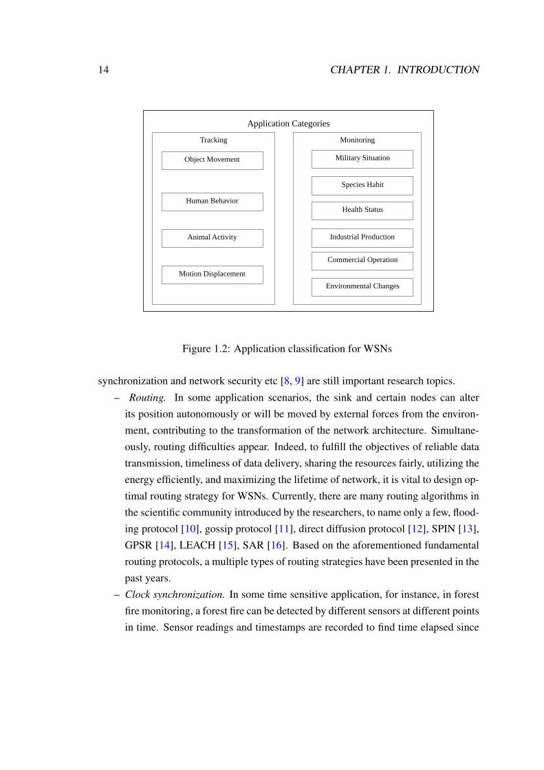
In a taxonomic manner, the utilization of WSNs can be mainly classified into twocategories: target tracking and event monitoring [5]. As described in Figure 1.2, tar-get tracking involves object movement tracking, observation of human behavior, animalactivity tracking, motion displacement calculation and so on. Similarly, the event mon-itoring comprises the following points: military situation surveillance, species habitobservation, health status monitoring, industrial process control, commercial operationsupervision, environmental changes perception etc.
1.1.3 Characteristics and focuses of WSNs
Promoted by the development of microelectronics, embedded systems and telecom-munication technologies, WSNs have gained increasing popularity in the humanity livesfor numerous applications. For example, sensors nodes can be integrated into a wire-less body area network (WBAN), a new enabling technology for health monitoring [6].Furthermore, the Internet of things (IOT), which is based on wireless sensor networks,makes it possible to access remote sensor data and to control the physical world from adistance [7].
The advance in technology enables miniaturization, low power consumption, lowcost, easy deployment and so on. Even if the technology is well developed, some issuesrelated to network topology, routing protocol, energy optimization, localization, clock
14 CHAPTER 1. INTRODUCTION
Application Categories
Tracking
Object Movement
Human Behavior
Animal Activity
Motion Displacement
Monitoring
Military Situation
Species Habit
Health Status
Commercial Operation
Industrial Production
Environmental Changes
Figure 1.2: Application classification for WSNs
synchronization and network security etc [8, 9] are still important research topics.
– Routing. In some application scenarios, the sink and certain nodes can alterits position autonomously or will be moved by external forces from the environ-ment, contributing to the transformation of the network architecture. Simultane-ously, routing difficulties appear. Indeed, to fulfill the objectives of reliable datatransmission, timeliness of data delivery, sharing the resources fairly, utilizing theenergy efficiently, and maximizing the lifetime of network, it is vital to design op-timal routing strategy for WSNs. Currently, there are many routing algorithms inthe scientific community introduced by the researchers, to name only a few, flood-ing protocol [10], gossip protocol [11], direct diffusion protocol [12], SPIN [13],GPSR [14], LEACH [15], SAR [16]. Based on the aforementioned fundamentalrouting protocols, a multiple types of routing strategies have been presented in thepast years.
– Clock synchronization. In some time sensitive application, for instance, in forestfire monitoring, a forest fire can be detected by different sensors at different pointsin time. Sensor readings and timestamps are recorded to find time elapsed since
1.2. LOCALIZATION IN WSNS 15
the fire was first spotted and its direction [17]. It is essential to maintain rigorousand uniform time schedule in these disaster monitoring applications. Pursue thetime synchronization rapidly and accurately is the anticipated direction on thisissue.
– Security. For most applications, security of datas or communication must be guar-anted. In a general way, no network can avoid this problem. In the state of theart of WSNs, hardware protection and software encryption, or the combination ofthe two methods, are employed. However, there are yet many challenging worksto be done on the security.
– Localization. In the previous section, we have seen that the localization of nodesis essential for numerous applications. As it is the main subject of our work, thistopic will be discussed in detail in the following sections.
In summary, there are still many issues in this field, that must be deep investigatedand are waiting scholars to further study.
1.2 Localization in WSNs
Wireless sensor networks have been applied in many military and civilian applica-tions to monitor environmental change and detect abnormal events [18]. Specifically,the node position information is essential to some localization sensitive applications.Determining the positions of sensor nodes precisely is a vital issue as the collected dataare closely related with the location information.
Researchers have made much efforts to solve the localization problem by adoptingother positioning systems into the WSNs. To sum up, the following means can beemployed:
– GPS– Cellular network– Infrared device– Ultrasonic wave– Micro inertial navigationA common feature shared in the above positioning strategies is that extra modules
are integrated in sensor nodes, which leads to increase the power consumption and com-munication overhead but also the deployment cost. To solve this problem, scholars tried

16 CHAPTER 1. INTRODUCTION
to acquire the location without additional devices by using only received signal infor-mation which can be available in the radio transceiver used for the communication. Thisinformation can be time of arrival (TOA), time difference of arrival (TDOA), angle ofarrival (AOA) and received signal strength indicator (RSSI) [19].
The advantages and disadvantages of these methods will be discussed in Chapter 2.The RSSI is the most common information, available in every transceiver. In this thesis,we have worked on solving indoor localization problems by using algorithms based onthe RSSI. As the RSSI is not an accurate parameter to determine distances, we haveworked on improving the localization accuracy of the proposed algorithms.
1.3 Thesis Contribution
In this dissertation, we focus on RSSI based localization algorithms for indoor ap-plications. The main contributions of this thesis involve the following three aspects.
1. Firstly, an experimental localization system has been built to get real RSSI data.From the measurements, a RSSI channel model has been deduced, which is con-sistent with the popular lognormal shadowing path loss model. Much more datahave been acquired to observe the relationship between the variance of noise anddistance. Based on the obtained data, it has been showed that the standard de-viation of the noise increases with the distance. To confirm this tendency, a raytracing system for an environment similar to the experimental environment, hasbeen used to simulate the receive and transmit process of RSSI data.
2. Secondly, we have proposed three novel indoor localization algorithms basedon multilateration and averaged RSSI, called Three minimum Distances Method(TDM), Weighted Three minimum distances Method (WTM) and Weight valuesAdjustment Method (WAM). These algorithms deal with the poor accuracy of thedistances deduced from RSSI. Using the experimental channel model deducedfrom measurements, the performance of the proposed algorithms has been veri-fied and compared in realistic conditions.
3. Finally, a RSSI based parameter tracking strategy for constrained position local-ization has been proposed. To estimate channel model parameters, Least MeanSquares method (LMS) has been associated with the trilateration method. In the

1.4. DISSERTATION STRUCTURE 17
context of applications where the positions are constrained on a grid, a noveltracking strategy has been proposed to determine the real position and obtain theactual parameters in the monitored region. The proposed tracking strategy hasalso been evaluated using the channel model deduced from the experimentations.
1.4 Dissertation structure
The dissertation is composed of 6 Chapters.
In Chapter 2, we introduce the state of the art of localization techniques in WSNs,including the extra modules aided and extra modules free approaches. Some impor-tant methods for our work such as linear least squares (LLS), non linear least squares(NLS), projection onto convex sets (POCS) and semidefinite programming (SDP) areparticularly detailed.
Chapter 3 deals with channel model which is a fundamental part of RSSI basedlocalization algorithms. An experimental channel model is deduced from RSSI dataacquired by a real localization system developed during this PhD work.
In Chapter 4, three localization methods: TDM, WTM and WAM are presented. Theaccuracy and calculation time of the proposed methods are compared with LLS, NLSand POCS.
The accuracy of the channel model is fundamental for the proposed RSSI basedlocalization algorithms. A parameter tracking strategy is proposed in Chapter 5 whichcan be applied to applications where the mobile positions are constrained to a grid.Quantitative criteria are provided to guarantee the efficiency of the proposed trackingstrategy by providing a tradeoff between the grid resolution and parameter variations.
Finally, the conclusion and future work directions are discussed in Chapter 6.
1.5 Conclusion
In this Chapter, we have firstly presented the main principles and applications ofWSNs and the induced research topics that remain important in that field. Then wehave introduced the problem of localization in WSNs. Finally, we have summarized themain contributions of our work and described structure of the thesis.

18 CHAPTER 1. INTRODUCTION
The following Chapter is dedicated to the state of the art of localization strategiesand particularly to the techniques which can be applied to WSNs.

2Localization strategies in WSNs
As mentioned in the previous chapter, for numerous applications of WSN, the local-ization of the nodes is a fundamental information which must be associated to the sensormeasurements. As a bridge between the physical world and the digital world, WSNsare widely used to deal with sensitive information in many fields. Application scenar-ios of WSNs include military, industrial, household, medical, marine and other fields,especially in natural disasters monitoring, early warning, rescuing and other emergencysituations. For example, by a smart dust network, suspended nodes in the air spacecan detect pressure, temperature and other information of different positions to monitorthe quality of the atmosphere. Sensor nodes buried under the bed at different depthscan collect temperature, pressure and other data to observe the activity of the glacier[20]. Sensor nodes in birds’ nests can help users to further research the living habits ofbirds [21]. In above mentioned applications, all collected information is based on theaccurate location of sensor nodes. Therefore, localization is one of the basic and coretechnologies in WSNs [22].
In this chapter, the localization principle and process are discussed. A classificationof localization strategies in WSNs is provided, and some typical approaches are revisitedand detailed.
19

20 CHAPTER 2. LOCALIZATION STRATEGIES IN WSNS
2.1 Localization process
The objective of a localization process is to determine the position of an object ofinterest through a specific system. According to the application specific requirements,appropriate algorithms can be chosen among existing localization techniques.
For applications which require only coarse localization, the position is obtained di-rectly, by determining the proximity to an anchor or by using hop count methods orfinger printing [23]. It should be noticed that coarse localization methods are simplemeans to provide an initial estimate for a more accurate localization method.
For applications requiring a better accuracy, the localization methods include twosteps: distance measurement and position calculation. As illustrated in Figure 2.1, thefirst block estimates distance or angles of arrival (AOA) from the received signal in-formation: time of arrival (TOA), time difference of arrival (TDOA), received signalstrength indication (RSSI) and other available features. The second stage processes thedistance and angular information and estimates the position through several positioningmethods associated with optimization approaches.
All the relevant measurement techniques mentioned above: TOA, TDOA, DOA,RSSI, and localization algorithms: Triangulation, Trilateration, Multilateration will bedescribed further.
Measurement
Techniques
Location
Calculation
Signal
Information
Measured Distances
Angles of Arrival Estimated
Position
Figure 2.1: Two steps of localization process
2.2 Localization strategies overview in WSNs
Numerous methods have been proposed for localization in WSNs. From a hardwareperspective, the positioning strategies can be divided into two categories: extra modules

2.3. EXTRA MODULES AIDED APPROACHES 21
aided approaches and extra modules free approaches, as illustrated in Figure 2.2.A detailed explanation of the two strategies will be addressed in the subsequent
section.
Localization
Strategies
Extra Modules
Aided Approaches
Extra Modules
Free Approaches
GPS Method
Cellular Network Method
Infrared Method
Ultrasonic Method
Micro Inertial Navigation Method
Range Based
Methods
Range Free
Methods
Connectivity
Geometry
Energy
AOA
TOA/TDOA
RSSI
Figure 2.2: Application classification for WSNs
2.3 Extra modules aided approaches
For this class of methods, a specific hardware is dedicated to the localization. Thisapproach includes GPS method, cellular network method, infrared method, ultrasonicwave method, micro inertial navigation method, to name just a few [24]. In the follow-ing, we will briefly address the above-mentioned localization techniques and discuss thecombination of these techniques and WSNs from a practical perspective.
22 CHAPTER 2. LOCALIZATION STRATEGIES IN WSNS
2.3.1 GPS method
The Global Positioning System, abbreviated as GPS, is a satellite based positioningsystem developed by the American military authorities in the 1970s. In the followingfour decades, GPS has been widely used in both military and civilian fields for naviga-tion, communications and monitoring. Similarly, the European Union and Russia havebuild their position systems, named Galileo and Glonass Systems respectively. In re-cent years, China has establishing the BeiDou Navigation Satellite System for pursuinga higher precision and extensive applications [25].
In order to accomplish the task of tracking the displacement of a sensor, GPS mod-ules can be integrated into the nodes. However, there exist some drawbacks and limita-tions in it. In some environments, like underground parking, underwater sites or indoorenvironments, GPS receiver can not communicate with the satellites [26]. Consequently,it is unfeasible to use GPS in these environments. Besides, high energy consumption isalso a drawback in employing GPS modules. Therefore, using GPS for localization inWSNs has some fundamental limitations, which make us steering to other techniques.
2.3.2 Cellular network method
A cellular network is a communication network where the last link is wireless andused for mobile communication. In that case it is an extra module free method becausethe cellular modem is also used for communication.
The Global System for Mobile Communication is abbreviated as GSM, is a standarddeveloped by the European Telecommunications Standards Institute (ETSI) to describethe protocols for second-generation digital cellular networks [27]. In the recent years,with the advent of third-generation and fourth-generation (4G) technologies, mobilecommunications went up to a higher level [28]. In cellular wireless location systems,a plurality of base stations receive signals from a mobile terminal simultaneously, andthen the cellular network accomplishes the localization process based on the measuredparameters.
In WSNs, the sensor nodes can be equipped with the relevant modules and localizedby cellular network . However, there are many limitations and drawbacks in this method.Most importantly, it provides an unsatisfactory localization precision, ranging from theorder of tens of meters to hundreds of meters. In addition, the cellular network module

2.3. EXTRA MODULES AIDED APPROACHES 23
is energy consuming, which contradicts the low cost objectives in WSNs. Therefore,there are still many multi-aspects and challenging issues in this direction to be fixed.
2.3.3 Infrared method
Infrared ray is another kind of electromagnetic wave, whose wavelength ranges fromthe microwave to the visible light wavelength. Due to its thermal effect and highlypenetrating ability, infrared ray is extensively used in medical treatment and industrialdetection and control. With the advance of microelectronics and optical fiber communi-cation, infrared transducer became a low cost device which can be employed for objectdetection and vehicle tracking [29].
When propagating in the space, the infrared ray would undergo deviations like re-flection, refraction, scattering, interference and absorption [30]. Due to these effects,it is nearly impossible to use infrared transducer into WSNs for localization when theenvironment is complex. On the contrary, the sensor nodes with infrared transducer inWSNs can be used with success for detection. To sum up, the use of infrared technologyfor localisation in WSNs remains an open issue.
2.3.4 Ultrasonic wave method
Ultrasonic wave is a part of sound waves, whose frequency is beyond 20kHz [31].Distinctly different from the ordinary sound waves, the ultrasonic wave has the follow-ing characteristics: superior directionality, longer transmission range, strong reflectivityand penetrability [32]. Due to the above-described features, the ultrasonic wave is in-troduced successfully into engineering and health-care fields.
The principle of ultrasonic wave based localization can be addressed concisely asfollows. The receiver estimates the time of arrival or the difference of time of arrivaland measures the propagation time t. The distance between the sender and receiver canbe estimated as (2.1):
s = vwt (2.1)
where vw is the velocity of the ultrasonic wave in the relevant transmission medium.
Since the ultrasonic wave suffers from interference and distortion in harsh environ-ment with a variety of obstructions, it is impractical to estimate displacement by means
24 CHAPTER 2. LOCALIZATION STRATEGIES IN WSNS
of ultrasonic wave based localization techniques extensively [32]. On the contrary, theultrasonic wave can propagate steadily in the water, which enables the ultrasonic wavebased localization techniques to some specific application fields. In the marine envi-ronment monitoring, ultrasonic wave based localization technique is considered as anadvisable method. Many researchers are trying to integrate ultrasonic module into sen-sor nodes and exploring the application in marine monitoring and navigation.
2.3.5 Micro inertial navigation method
Mainly based upon the acceleration sensor, direction sensor and gyroscope sensor,micro inertial navigation is identified as an accurate navigation system estimating themovement parameters from the data sensed by the above mentioned devices. A distinctfeature is its independent estimation, namely, the localization process uses only inter-nal equipment without the help of outside systems [33]. This technique is originallyemployed for missile guidance, and then aircraft and submarine navigation.
To overcome the limitations in GPS system and improve the localization accuracy,the researchers introduced the micro inertial navigation method into WSNs. In the pro-cess of movement, the acceleration sensor obtains the acceleration of the node move-ment and the orientation sensor obtains the node posture instantaneously. After theacceleration data and the direction angles of the node are acquired, the displacementof the node’s movement can be calculated through integral calculation. Micro inertialnavigation system provides a satisfying accuracy in short term but can exhibit deviationin long period. So, it can be used in addition to other localization systems (GPS or cel-lular networks) when they become periodically unavailable. Despite that micro inertialnavigation can gain a higher precision in short range, a heavy energy consumption isinevitable. Therefore, it is imperative to make a trade-off in practical applications tomeet the diverse requirements [34].
2.4 Extra modules free approaches
Compared to the extra modules aided approaches, extra modules free approachesrequire no additional components to assist the localization process. Namely, rather thansupported by external localization systems and internal mounted components, the ex-

2.4. EXTRA MODULES FREE APPROACHES 25
tra modules free approaches carry out the localization task merely by its own networkparameters.
Extra modules free approaches are typically divided into two aspects: range freemethods and range based methods [35]. Compared to range-free localization, range-based localization provides higher precision. There are many range-based localizationtechniques, such as those based on the measurement of TOA [36, 37], AOA [38, 39],TDOA [40, 41], RSSI [42] and so on.
RSSI-based algorithms have the following characteristics: low power consumption,simple hardware but high sensitivity to environment. RSSI value heavily depends onthe propagation channel. Signal reflection, multipath propagation, noise and signal scat-tering have great influence on the received RSSI. Therefore, in practical applications,establishing an accurate channel model to deduce the distance from the received RSSIvalue is crucial to the performance of localization algorithms.
An in depth explanation for the two types of methods will be addressed in the fol-lowing section.
2.4.1 Range free methods
Contrary to range-based algorithms, range-free algorithms accomplish localizationthrough network and devices features, such as network connectivity graph, device powerconsumption and conservation, geometric relationship and many more, instead of rang-ing the distance between target and anchor nodes. In the sequel, several classical local-ization algorithms: distance vector hop (DV hop) [43], approximate point-in-triangulationtest (APIT) [44] and centroid algorithm [45], will be revisited.
2.4.1.1 DV hop
Inspired by the classical distance vector routing scheme, DV-Hop algorithm is pro-posed in [46]. It involves three steps in the localization process as follows:
1. In the initial step, an information table is built for each node according to the land-mark broadcast location and hop data. The data package is exchanged betweennode and its neighbors. The table is denoted as (xi, yi, hi), where (xi, yi) is thecoordinates of the ith landmark and hi is the minimum hop count value from theith landmark to the target node who maintains this table.
26 CHAPTER 2. LOCALIZATION STRATEGIES IN WSNS
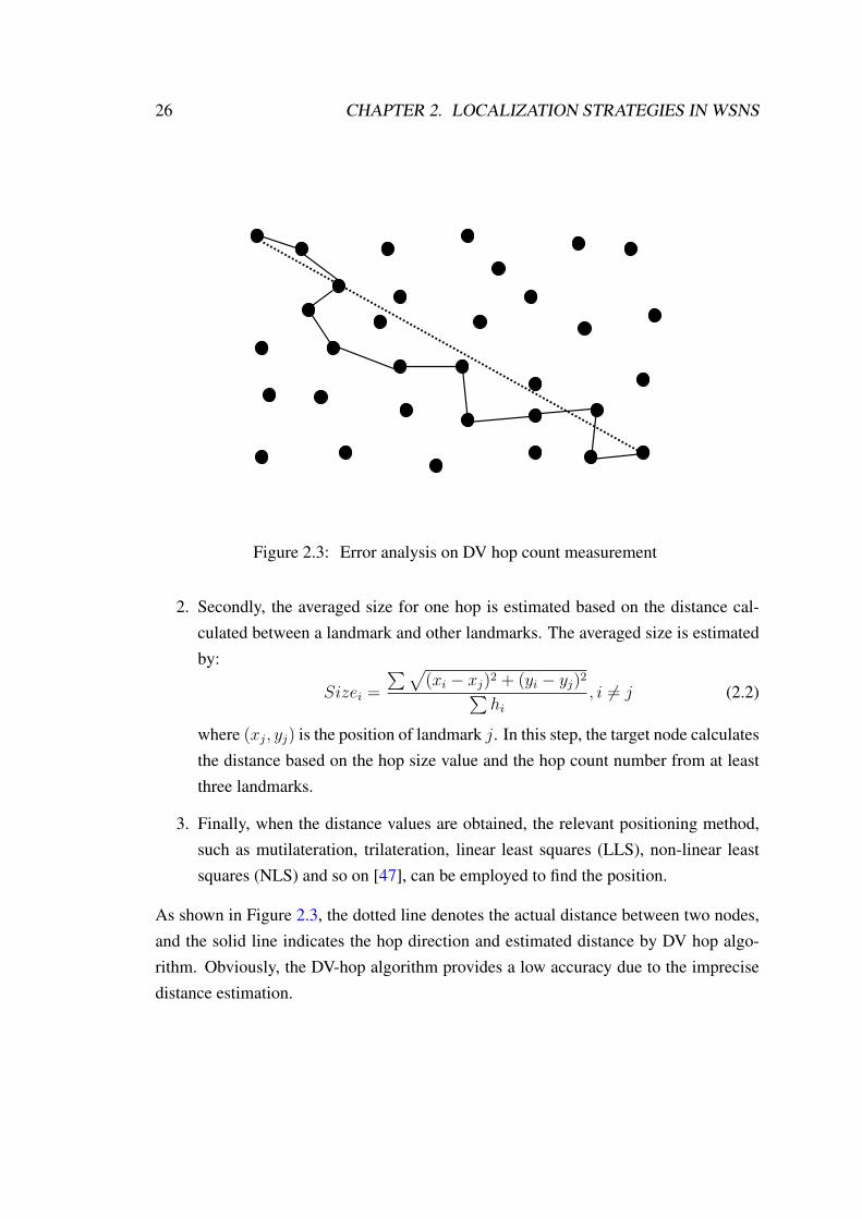
Figure 2.3: Error analysis on DV hop count measurement
2. Secondly, the averaged size for one hop is estimated based on the distance cal-culated between a landmark and other landmarks. The averaged size is estimatedby:
Sizei =
∑√(xi − xj)2 + (yi − yj)2∑
hi, i 6= j (2.2)
where (xj, yj) is the position of landmark j. In this step, the target node calculatesthe distance based on the hop size value and the hop count number from at leastthree landmarks.
3. Finally, when the distance values are obtained, the relevant positioning method,such as mutilateration, trilateration, linear least squares (LLS), non-linear leastsquares (NLS) and so on [47], can be employed to find the position.
As shown in Figure 2.3, the dotted line denotes the actual distance between two nodes,and the solid line indicates the hop direction and estimated distance by DV hop algo-rithm. Obviously, the DV-hop algorithm provides a low accuracy due to the imprecisedistance estimation.

2.4. EXTRA MODULES FREE APPROACHES 27
A high density nodes deployment can provide a better accuracy. However, owing toits simplicity, this method can be applied into some rough localization.
2.4.1.2 APIT
APIT is a range free localization algorithm, presented in [48]. The core idea ofthis method is to associate Point-In-Triangulation Test (PIT) with area-based schemeto search the most likely target position. PIT is adopted for narrowing the possibleregion where the target is located. We assume that many anchor nodes, whose locationis known by other means, are scattered in a wireless sensor networks. As illustratedin Figure 2.4, in every trial, three anchors are selected to form a triangle and whetherthe position of the target is in this triangle or not is decided. This process is repeateduntil all the triangles are considered. After finishing all the tests, the center point ofintersection area will be regarded as the estimated position. The localization accuracyof APIT depends on the test number which is directly related with the anchor number.Unavoidably, the power and time consumptions increase with number of anchors [49].
Figure 2.4: Principle of APIT algorithm
28 CHAPTER 2. LOCALIZATION STRATEGIES IN WSNS
2.4.1.3 Centroid algorithm
Centroid localization algorithms estimate the position via geometric relationship be-tween the landmarks and the unknown nodes, instead of calculating the correspondingdistance. These algorithms are suitable for the wireless sensor networks with a certainnumber of landmarks whose positions are recognized by other complementary schemes.Periodical packets containing position information are broadcasted among the networks.When the number of received packets exceed a predefined threshold value, a stabletransmission link is established between a node and a landmark. An unknown nodewill be connected with many landmarks. Assuming that the number of landmarks ismore than 3, a polygon is formed by these landmarks. Then, the centroid position isconsidered as the unknown node location.
As illustrated in Figure 2.5, scholars presented centroid localization algorithm basedon tetrahedron. A tetrahedron is limited by four anchor nodes L1, L2, L3, L4, whichare connected with the target to be localized. Then, the centroid of this tetrahedronis considered as the coordinates of the target. In [50], simulations were performed tocompare this method and the classical centroid algorithm. The results indicate that thetetrahedron algorithm gives a higher accuracy than the traditional method in spite thatlarger calculation time is required due to many estimation rounds. Other researchers in[51, 52, 53, 54] tried to improve the centroid algorithm by assigning weighted factors toeach anchors or associating correction schemes to reduce the localization error.
2.4.2 Range based methods
Contrary to the previous methods, range based methods perform position computa-tion after distance estimation. These methods involves two stages: distance measure-ment and position calculation.
Many techniques have been employed for distance measurement, for example, thetechniques based on time of arrival (TOA), time difference of arrival (TDOA), angle ofarrival (AOA) and received signal strength indicator (RSSI) [55]. After acquiring thedistance measurement, geometric relationship is used to compute the node position bytriangulation, multilateration, trilateration, hyperbolic and so on.
In the next section, these techniques are discussed in detail.

2.4. EXTRA MODULES FREE APPROACHES 29
1L
2L
3L
4L
M
O
D
Figure 2.5: Diagram of tetrahedron algorithm
2.4.2.1 Distance measurement techniques
Firstly, we will present the methods that can be used for the distance measurementstep. These methods are based on the measurement of the angle or distance, includingTOA, TDOA, RSSI and AOA.
TOA
In TOA and TDOA methods, the distance is ranged from the transmission time be-tween the transmitter and the receiver [56]. The time of flight (TOF) recorded betweentwo terminals can be is used to estimate the distance by a simple multiplication by thetransmitting velocity. The schemes for measuring elapsed time are classified into twocategories: one-way scheme and two-way scheme.
In one-way scheme, the transmitter sends signal to the receiver and the time delay
30 CHAPTER 2. LOCALIZATION STRATEGIES IN WSNS
for this transmission is measured. The transmitter sends message at time t1 and thereceiver gets the message at time t2. Then a decoding delay or synchronization time tcis required to accomplish the time record.
Therefore, the time delay τ can be written:
τ = (t2 + tc)− t1 (2.3)
The one-way scheme is simpler, but it is essential to synchronize the two termi-nal clocks to reduce the errors. High accurate clock synchronization is a challengingtask and clock bias results in measurement errors. This remark explains why two-wayscheme is generally privileged.
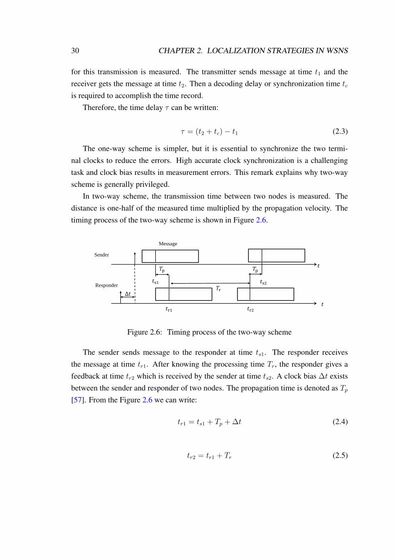
In two-way scheme, the transmission time between two nodes is measured. Thedistance is one-half of the measured time multiplied by the propagation velocity. Thetiming process of the two-way scheme is shown in Figure 2.6.
Sender
Responder 𝑡s1 𝑡s2
𝑡r1 𝑡r2
𝑡
𝑇r
𝑇p 𝑇p
Message
𝑡
∆𝑡
Figure 2.6: Timing process of the two-way scheme
The sender sends message to the responder at time ts1. The responder receivesthe message at time tr1. After knowing the processing time Tr, the responder gives afeedback at time tr2 which is received by the sender at time ts2. A clock bias ∆t existsbetween the sender and responder of two nodes. The propagation time is denoted as Tp[57]. From the Figure 2.6 we can write:
tr1 = ts1 + Tp + ∆t (2.4)
tr2 = tr1 + Tr (2.5)

2.4. EXTRA MODULES FREE APPROACHES 31
Finally,ts2 = tr2 + Tp −∆t (2.6)
Then by subtracting ts2 and ts1, we get the result
ts2 − ts1 = 2Tp + Tr. (2.7)
Then time Tp can be calculated by
Tp =ts2 − ts1 − Tr
2. (2.8)
As shown in the previous equation, the clock bias ∆t is eliminated by this process.
In two-way scheme, the transmission time is obtained by recording packet receivingand sending times. In spite that this two-way scheme does not need clock synchroniza-tion, inaccurate packet processing time in terminals results in measurement errors.
An alternative method called TDOA is proposed to measure time difference betweentwo propagation processes [58]. A typical TDOA system will be discussed in detail inthe following.
TDOA
The key concept of TDOA-based localization technique is to determine the locationof the source by evaluating the difference in arrival time of the signal at spatially sepa-rated base stations [59]. As shown in Figure 2.7, there are three signal receivers: RX1,RX2, and RX3, whose coordinates are known as (x1, y1), (x2, y2) and (x3, y3). The ob-jective is to determine the position of the transmitter with unknown coordinates (x, y).The reception times in RX1, RX2 and RX3 are respectively t1, t2 and t3. This valuescan be combined to obtain the following equation [60]:
√(x− x2)2 + (y − y2)2 −
√(x− x1)2 + (y − y1)2 = c× (t2 − t1)√
(x− x3)2 + (y − y3)2 −√
(x− x1)2 + (y − y1)2 = c× (t3 − t1)(2.9)
where c is the speed of light.
By solving the above nonlinear equations, the position of TX can be determined.

32 CHAPTER 2. LOCALIZATION STRATEGIES IN WSNS
RX2
TX
RX1 RX3
(𝑥1, 𝑦1 )
(𝑥2, 𝑦2 )
(𝑥3, 𝑦3 ) 𝑡1
𝑡2
𝑡3
Figure 2.7: Terminals deployment of TDOA method
The main drawback of the TDOA technique is that the reception time difference canbe fairly small, especially in short distance measurement, and the distance estimationis not precise [61]. To overcome this problem, the electromagnetic waves can be re-placed by acoustic waves. The propagation velocity is much smaller and thus the timedifferences are largely increased.
As seen in Figure 2.8, ultrasound/acoustic and RF modules are simultaneously usedin transmitter and receiver. The principle is to measure the time difference between thepropagation times of the acoustic and radio signals [62].
In the initial localization step, the transmitter sends at time t0 the radio signal whichis received by the receiver at time tradio. After a fixed time delay tdelay, the transmittersends the acoustic signal which is received at time tsound. Figure 2.9 shows the timedelay computation model for this type of TDOA [63]. The two received times can bewritten :
tradio = t0 +d
vradio(2.10)
andtsound = t0 + tdelay +
d
vsound(2.11)
where d is the distance between the transmitter and the receiver and vradio and vsound
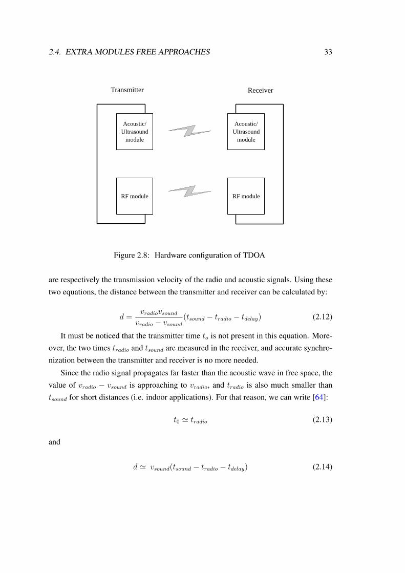
2.4. EXTRA MODULES FREE APPROACHES 33
Acoustic/
Ultrasound
module
Acoustic/
Ultrasound
module
RF module RF module
Transmitter Receiver
Figure 2.8: Hardware configuration of TDOA
are respectively the transmission velocity of the radio and acoustic signals. Using thesetwo equations, the distance between the transmitter and receiver can be calculated by:
d =vradiovsoundvradio − vsound
(tsound − tradio − tdelay) (2.12)
It must be noticed that the transmitter time to is not present in this equation. More-over, the two times tradio and tsound are measured in the receiver, and accurate synchro-nization between the transmitter and receiver is no more needed.
Since the radio signal propagates far faster than the acoustic wave in free space, thevalue of vradio − vsound is approaching to vradio, and tradio is also much smaller thantsound for short distances (i.e. indoor applications). For that reason, we can write [64]:
t0 ' tradio (2.13)
and
d ' vsound(tsound − tradio − tdelay) (2.14)

34 CHAPTER 2. LOCALIZATION STRATEGIES IN WSNS
where tsound and tradio are measured at the receiver. There is no need to synchronize thetransmitter and receiver.
Transmitter
Receiver
Acoustic RF
t𝑟𝑎𝑑𝑖𝑜
t𝑑𝑒𝑙𝑎𝑦
t𝑠𝑜𝑢𝑛𝑑
t0
Figure 2.9: Time delay computation model for TDOA
RSSI
The RSSI, which denotes the Received signal strength indicator, is a measurement ofthe receiver signal power. It is available in most of receivers and can be used for distancemeasurement as it can be expected that its value decreases with the distance [65]. ManyRSSI based algorithms have been presented for unknown target localization in wirelesssensor networks. To characterize the relationship between the received signal strengthand transmission distance, several path loss models are built based on experimental data.In free space propagation, the relationship between signal strength and transmissiondistance is expressed by Friis equation as [66]:
Pr(d) =PtGtGrλ
2
4π2dηL, (2.15)
where– Pr and Pt are respectively the received and transmit powers,– Gt and Gr are the antenna gains of the transmitter and receiver,– L is the system loss,– d is the radio transmission distance,– η is the path loss exponent equal to 2 for free space,

2.4. EXTRA MODULES FREE APPROACHES 35
– λ is the radio wavelength defined by
λ =c
f(2.16)
where c is the light speed and f is the signal frequency.
For simplicity, the values of Gt, Gr and L are set to 1. Equation (2.15) is simplifiedto:
Pr(d) =Ptλ
2
4π2dη(2.17)
From the relationship between the transmitted and received powers, we can definethe path loss PL which denotes the power attenuation during the propagation [67]:
PL =PtPr
= (2π
λ)2dη (2.18)
Substituting (2.16) into (2.18), we get:
PL =PtPr
= (2π
c)2f 2dη (2.19)
This equation indicates that the pass loss is determined by two factors: radio fre-quency f and transmission distance d. Path loss increases with frequency f and distanced.
The path loss exponent η is determined by the transmission environment. In usualenvironments, the free space assumption is no longer verified. Multi-path and shadow-ing have great impact on factor η. A large number of experiments indicate that the valueof η is generally between 2 and 4 [68].
A simplified formula for RSSI computation is proposed in [69]:
Pr =Pt(d0)
dη(2.20)
where d0 is a reference distance usually equals to one meter. On the study of the receivedpower in the receiver, the relation between RSSI and distance is interpreted as [70]:
Pr(d) = Pr(d0) + 10ηlog(d
d0) +Xσ (2.21)
36 CHAPTER 2. LOCALIZATION STRATEGIES IN WSNS
where the powers are expressed in dBm and Xσ is zero mean Gaussian distributed ran-dom variable whose mean value is zero. This variable reflects the local variations of thereceived power due to fading and shadowing [71].
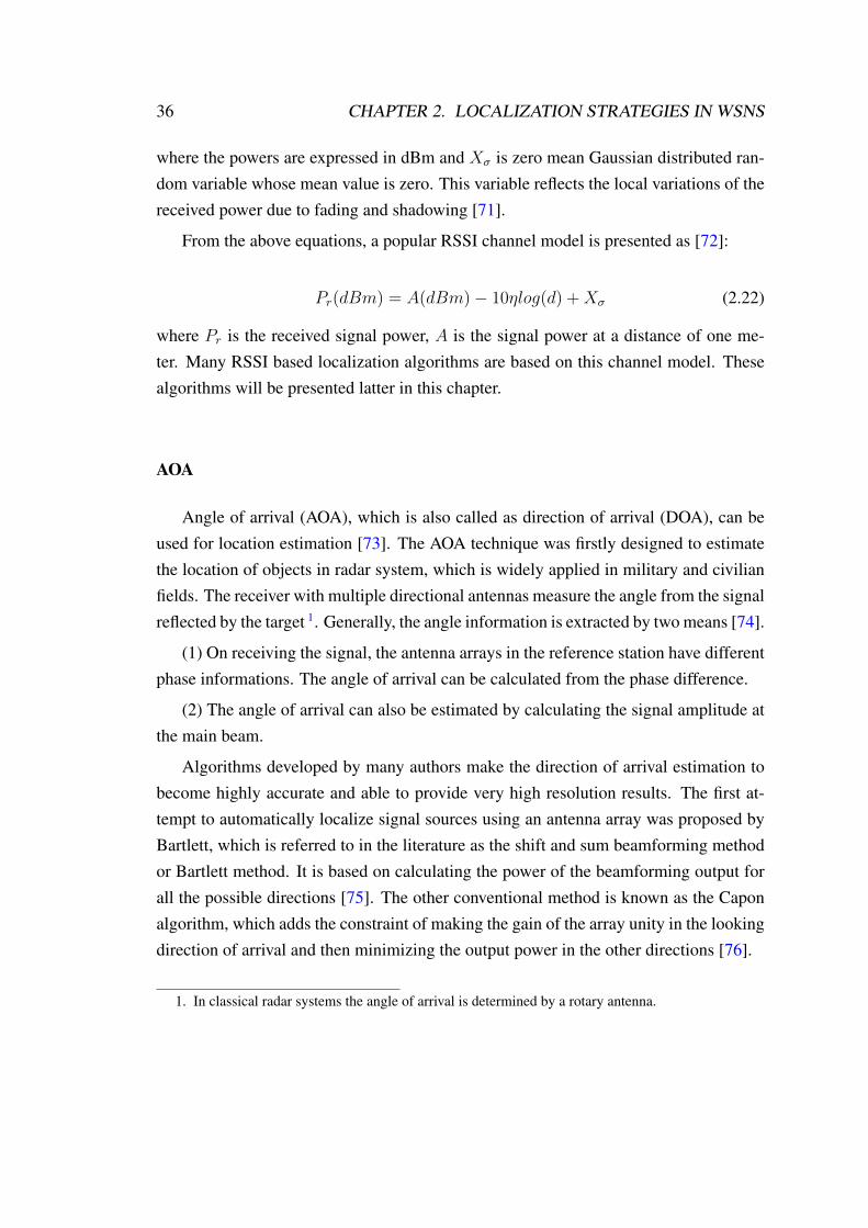
From the above equations, a popular RSSI channel model is presented as [72]:
Pr(dBm) = A(dBm)− 10ηlog(d) +Xσ (2.22)
where Pr is the received signal power, A is the signal power at a distance of one me-ter. Many RSSI based localization algorithms are based on this channel model. Thesealgorithms will be presented latter in this chapter.
AOA
Angle of arrival (AOA), which is also called as direction of arrival (DOA), can beused for location estimation [73]. The AOA technique was firstly designed to estimatethe location of objects in radar system, which is widely applied in military and civilianfields. The receiver with multiple directional antennas measure the angle from the signalreflected by the target 1. Generally, the angle information is extracted by two means [74].
(1) On receiving the signal, the antenna arrays in the reference station have differentphase informations. The angle of arrival can be calculated from the phase difference.
(2) The angle of arrival can also be estimated by calculating the signal amplitude atthe main beam.
Algorithms developed by many authors make the direction of arrival estimation tobecome highly accurate and able to provide very high resolution results. The first at-tempt to automatically localize signal sources using an antenna array was proposed byBartlett, which is referred to in the literature as the shift and sum beamforming methodor Bartlett method. It is based on calculating the power of the beamforming output forall the possible directions [75]. The other conventional method is known as the Caponalgorithm, which adds the constraint of making the gain of the array unity in the lookingdirection of arrival and then minimizing the output power in the other directions [76].
1. In classical radar systems the angle of arrival is determined by a rotary antenna.

2.4. EXTRA MODULES FREE APPROACHES 37
2.4.2.2 Location calculation
In the previous section, the methods to estimate the angle or distance, have beendiscussed. However, these informations need to be further processed by positioningalgorithms to find the coordinates of the object.
The objective of the following sections is to present the algorithms that can be usedto calculate the position, such as Triangulation, Multilateration, Trilateration, linearleast squares (LLS), non linear least squares (NLS), projection onto convex sets (POCS)and semidefinite programming (SDP) [77].
Triangulation
T
(x, y)
BS
θ𝑖
X
Y
(x𝑖 , y𝑖)
Figure 2.10: Angle of arrival measurement.
When the angle of arrival is obtained, triangulation algorithm can be used for loca-tion estimation. As illustrated in Figure 2.10, the transmitter T sends signal to the basestation i. The angle of arrival θi is given by:
tanθi = (y − yix− xi
) (2.23)
where (xi, yi) is the coordinates of the base station i; (x, y) is the coordinates of trans-

38 CHAPTER 2. LOCALIZATION STRATEGIES IN WSNS
mitter T.
In triangulation, at least two base stations are needed for two-dimensional localiza-tion. The principle of triangulation is shown in Figure 2.11. The location of transmitterT can be computed from the two angles θ1 and θ2 by:
T
(x, y)
BS1
θ1
X
Y
(x1, y1) BS2 (x2, y2)
θ2
Figure 2.11: Triangulation
x =L tan(θ2)
tan(θ2)− tan(θ1)
y =L tan(θ1)tan(θ2)
tan(θ2)− tan(θ1)
(2.24)
where L is the distance between the two base stations, which can be calculated by:
L =√
(x1 − x2)2 + (y1 − y2)2 (2.25)
The accuracy of triangulation relies heavily on the measured angle of arrival. Im-proving the measurement precision on arrived direction is a way to guarantee a higheraccuracy. Meanwhile, employing more base stations can also enhance the localizationperformance.

2.4. EXTRA MODULES FREE APPROACHES 39
Compared to TOA method, AOA method has the following advantages. Time syn-chronization is not required for measuring angle of arrival. The error caused by timemeasurement inaccuracy is avoidable. Less base stations are needed to estimate the po-sition in triangulation method. To find the position of one target, AOA needs two basestations but TOA needs at least three base stations with known position. Moreover, basestations can measure the arrived angle from the target without the cooperation of thetarget, which reduces the communication overhead and makes the localization processless complex.
However, the drawback in AOA method may cause some limitations when it is ap-plied in practical localization process. When the distance between the target and basestation is large, the measured angle value is not accurate due to the varying transmissioncharacteristics in long path. It is hard to overcome this problem and the localizationperformance is reduced. Meanwhile, directional antennas or antenna array in base sta-tions will bring additional cost for localization system. In view of these features, AOAmethod is more applicable in radar localization system.
Multilateration
Multilateration is a popular method for finding the position of a target. In thismethod, at least three anchor nodes are needed for 2-D space localization. The equationsfor multilateration is expressed as:
(x− x1)2 + (y − y1)2 = d21
(x− x2)2 + (y − y2)2 = d22...
......
(x− xN)2 + (y − yN)2 = d2N
(2.26)
where (x, y) is the coordinates of the reference or unknown nodes, (x1, y1), (x2, y2),· · · , (xN , yN) are the coordinates of the N anchors. Then, this non-linear system ofequations must be solved by adequate methods to obtain the unknowns x and y.
In real environment, the distance measured from signal information is inaccurate dueto multi-path, reflection, shadowing and noise impact. Consequently, the position of thetarget can not be calculated exactly by multilateration. To find an optimal position,

40 CHAPTER 2. LOCALIZATION STRATEGIES IN WSNS
LLS, NLS and POCS methods have been employed and associated with multilateration.These methods will be elaborated in the following sections.
Trilateration
Anchor nodes
(x1, y1)
Unknown node
(x2, y2)
(x3, y3) (x, y)
Figure 2.12: Trilateration
As shown in Figure 2.12, when the number of anchors is 3, the multilateration is alsocalled trilateration. Under minimum anchor configuration, the position can be foundfrom three anchors, if they are not deployed in straight line. The relationship betweenthe unknown node and three anchor nodes is written by [78]:
(x− x1)2 + (y − y1)2 = d21
(x− x2)2 + (y − y2)2 = d22
(x− x3)2 + (y − y3)2 = d23
(2.27)
where (x, y) are the coordinates of the reference or unknown nodes, (x1, y1), (x2, y2),(x3, y3) are the coordinates of the three anchors. By subtracting the first equation tothe others, the system of equations (2.27) can be transformed into the following matrix
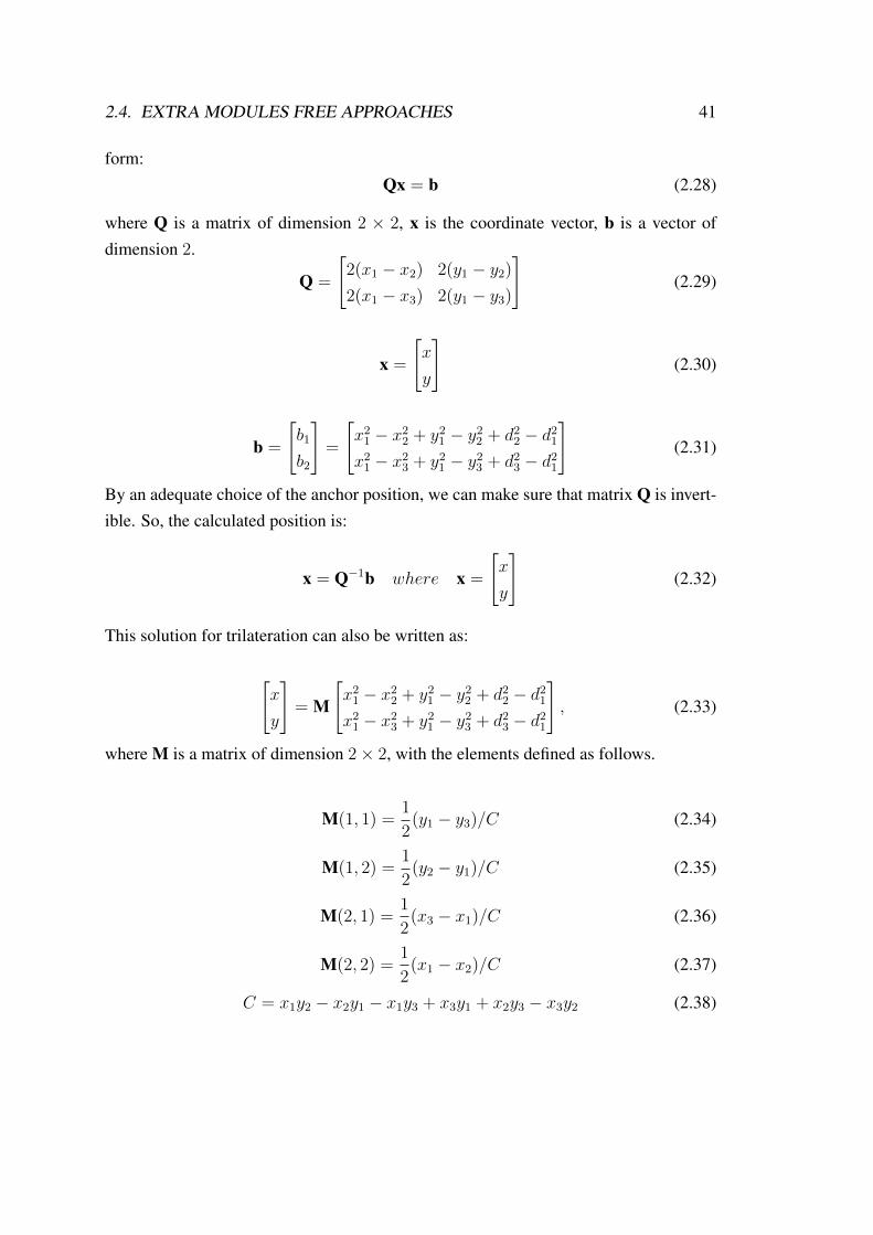
2.4. EXTRA MODULES FREE APPROACHES 41
form:Qx = b (2.28)
where Q is a matrix of dimension 2 × 2, x is the coordinate vector, b is a vector ofdimension 2.
Q =
[2(x1 − x2) 2(y1 − y2)2(x1 − x3) 2(y1 − y3)
](2.29)
x =
[x
y
](2.30)
b =
[b1
b2
]=
[x21 − x22 + y21 − y22 + d22 − d21x21 − x23 + y21 − y23 + d23 − d21
](2.31)
By an adequate choice of the anchor position, we can make sure that matrix Q is invert-ible. So, the calculated position is:
x = Q−1b where x =
[x
y
](2.32)
This solution for trilateration can also be written as:
[x
y
]= M
[x21 − x22 + y21 − y22 + d22 − d21x21 − x23 + y21 − y23 + d23 − d21
], (2.33)
where M is a matrix of dimension 2× 2, with the elements defined as follows.
M(1, 1) =1
2(y1 − y3)/C (2.34)
M(1, 2) =1
2(y2 − y1)/C (2.35)
M(2, 1) =1
2(x3 − x1)/C (2.36)
M(2, 2) =1
2(x1 − x2)/C (2.37)
C = x1y2 − x2y1 − x1y3 + x3y1 + x2y3 − x3y2 (2.38)

42 CHAPTER 2. LOCALIZATION STRATEGIES IN WSNS
Hyperbolic method
When the distances from the base stations to the target are obtained, the hyperbolicmethod can also be used to calculate the position of the target by mathematical relation-ship [79]. In geometry, there is a condition that the distance difference from one pointto other two predefined points is a constant. All points meeting this condition will forma hyperbola. On the basis of hyperbola principle, two base stations can be set on twofoci and the target is contained in the hyperbola.
T
(x, y)
BS1 (x1, y1)
BS2
(x2, y2)
d1 d2
Figure 2.13: Hyperbolic method
As shown in Figure 2.13, two base stations are on two foci of hyperbola. Theircoordinates are (x1, y1) and (x2, y2). The position of the transmitter to be localized isdenoted as (x, y). The relationship among the related positions are listed as follows:
x2
a2− y2
b2= 1 (2.39)
a2 = (∆d
2)2 (2.40)
b2 = (D
2)2 − a2 (2.41)
where a and b are two parameters for hyperbola equation, which can be provided by themeasured distances. D is the distance between the two base stations. ∆d is the distance
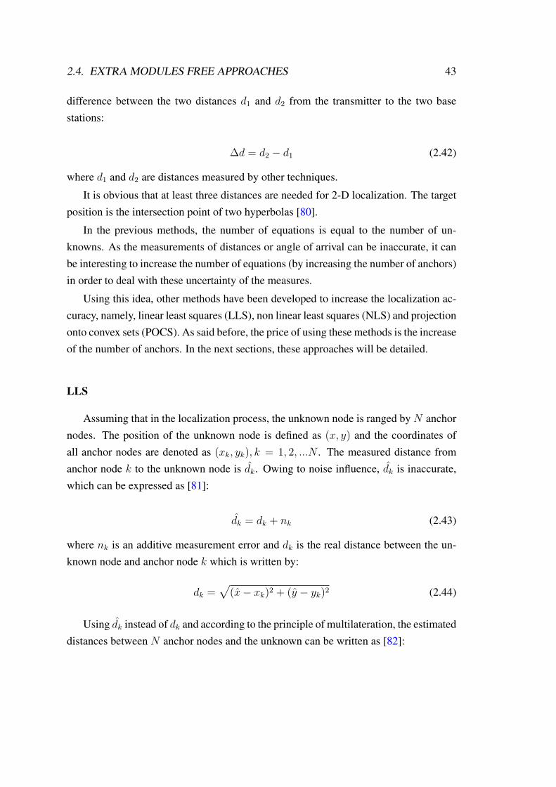
2.4. EXTRA MODULES FREE APPROACHES 43
difference between the two distances d1 and d2 from the transmitter to the two basestations:
∆d = d2 − d1 (2.42)
where d1 and d2 are distances measured by other techniques.
It is obvious that at least three distances are needed for 2-D localization. The targetposition is the intersection point of two hyperbolas [80].
In the previous methods, the number of equations is equal to the number of un-knowns. As the measurements of distances or angle of arrival can be inaccurate, it canbe interesting to increase the number of equations (by increasing the number of anchors)in order to deal with these uncertainty of the measures.
Using this idea, other methods have been developed to increase the localization ac-curacy, namely, linear least squares (LLS), non linear least squares (NLS) and projectiononto convex sets (POCS). As said before, the price of using these methods is the increaseof the number of anchors. In the next sections, these approaches will be detailed.
LLS
Assuming that in the localization process, the unknown node is ranged by N anchornodes. The position of the unknown node is defined as (x, y) and the coordinates ofall anchor nodes are denoted as (xk, yk), k = 1, 2, ...N . The measured distance fromanchor node k to the unknown node is dk. Owing to noise influence, dk is inaccurate,which can be expressed as [81]:
dk = dk + nk (2.43)
where nk is an additive measurement error and dk is the real distance between the un-known node and anchor node k which is written by:
dk =√
(x− xk)2 + (y − yk)2 (2.44)
Using dk instead of dk and according to the principle of multilateration, the estimateddistances between N anchor nodes and the unknown can be written as [82]:
44 CHAPTER 2. LOCALIZATION STRATEGIES IN WSNS
(x− x1)2 + (y − y1)2 = d21 (2.45)
(x− x2)2 + (y − y2)2 = d22 (2.46)
.
.
.
(x− xN)2 + (y − yN)2 = d2N (2.47)
where (x, y) is the estimated position and d1, d2, ..., dN are the measured distances.
Similarly to the trilateration method, these equations are rewritten as [83]:
x21 − x22 − 2(x1 − x2)x+ y21 − y22 − 2(y1 − y2)y = d21 − d22 (2.48)
x21 − x23 − 2(x1 − x3)x+ y21 − y23 − 2(y1 − y3)y = d21 − d23 (2.49)
.
.
.
x21 − x2N − 2(x1 − xN)x+ y21 − y2N − 2(y1 − yN)y = d21 − d2N (2.50)
These equations can be transformed into the following matrix form [84]:
Q1x = b (2.51)
where Q1 is a matrix of dimension (N − 1)× 2, x is the coordinate vector, b is a vectorof dimension (N − 1).

2.4. EXTRA MODULES FREE APPROACHES 45
Q1 =
2(x1 − x2) 2(y1 − y2)2(x1 − x3) 2(y1 − y3)
......
2(x1 − xN) 2(y1 − yN)
(2.52)
x =
[x
y
](2.53)
b =
x21 − x22 + y21 − y22 + d22 − d21x21 − x23 + y21 − y23 + d23 − d21
...x21 − x2N + y21 − y2N + d2N − d21
(2.54)
We obtain an overdetermined system (N−1) equations and two unknowns with N > 3.Equation (2.51) can be solved by the following linear least squared problem [85]:
Min‖Q1x− b‖2 (2.55)
The solution is given by:
x = (QT1 Q1)
−1QT1 b where x =
[x
y
](2.56)
(x, y) is the best position obtained by LLS.
NLS
This localization issue can be also settled by nonlinear least squares (NLS) approach[86]. Considering that the N anchors are included in the networks and their positionsare known as xk = (xk, yk), the cost function of the NLS method is expressed as:
x = arg minx∈R2
N∑k=1
[‖x− xk‖ − dk]2 (2.57)

46 CHAPTER 2. LOCALIZATION STRATEGIES IN WSNS
D1
D2
D3
D4
D
Figure 2.14: Projection onto Convex Sets
where (xk, yk) is the center position of each circle and dk is the estimated distancecorresponding to each circle.
The meaning of this optimization problem is that we want to minimize the squareerror between the estimated distances and the distances between anchors and node. Tosolve this minimization function defined by (2.57), interior point method, sequentialquadratic programming method (SQP), trust region reflective method, active set methodand so on can be selected and employed [87].
POCS
A shortcoming of NLS method is the possible inaccuracy caused by the existence ofsaddle points and local minimums [88]. To search the optimal position in the possibleareas, an alternative called projection onto convex sets (POCS) method is applied intotarget localization .

2.4. EXTRA MODULES FREE APPROACHES 47
According to the previous assumption, the N anchor nodes estimate the distanceto the target. N circles with center (xk, yk) are generated by anchor nodes. For eachmeasured distance, a disc can be defined as:
Dk = {x ∈ R2 ‖x− xk‖ ≤ dk k = 1, 2..., N} (2.58)
Generally, the target is located in the intersection region of the N discs. The inter-section region is defined by:
x ∈ D =⋂
k=1,2...,N
Dk (2.59)
The localization problem is searching a position in this intersection region, whichis denoted as D, as shown in Figure 2.14. As for this set D, in the presence of mea-surement noise, set D is equal to ∅. Considering this possible condition, the optimalposition estimated by POCS minimizes the sum distances to sets Dk. The minimizationformulation is expressed as [89]:
x = arg minx∈R2
N∑k=1
‖x− PDk(x)‖ (2.60)
where PDk(x) is the orthogonal projection of x onto sets Dk, defined as:
PDk(x) = arg minyk∈R2
N∑k=1
‖x− yk‖ (2.61)
where yk denotes all the points determined by the estimated distance dk.
Similarly, to solve the minimization function defined by (2.60), interior point method,sequential quadratic programming method (SQP), trust region reflective method, activeset method and so on can be selected and employed.
SDP
SDP relaxation can also be applied to solve the localization problem in wireless sen-sor works [90]. In the localization problem, non-convex constraints will give difficultiesin optimization and reduce the localization accuracy. These constraints can be relaxedinto semidefinite program which can approximate the position efficiently. According to

48 CHAPTER 2. LOCALIZATION STRATEGIES IN WSNS
the above definition, the relationship between the unknown node position x and anchornodes position xk is expressed as [91]:
‖ x− xk ‖2= d2k k = 1, 2..., N (2.62)
where x and xk are denoted as:
x =
[x
y
](2.63)
xk =
[xk
yk
](2.64)
The minimization formulation is expressed as:
x = arg minx∈R2
N∑k=1
[‖x− xk‖ − dk]2 (2.65)
The constraints defined by (2.62) can also be written as matrix form:
(−xk
1
)T( I2 xxT g
)(−xk
1
)= d2k (2.66)
where I2 is an identity matrix with dimension 2× 2, which is written as:
I2 =
(1 0
0 1
)(2.67)
and g is defined as:g = xTx = x2 + y2 (2.68)
Relax the above equations into a semidefinite program: change the constraint g =
xTx in (2.68) to g � xTx. This expression can be also modified as:
Z =
(I2 xxT g
)� 0 (2.69)
Equation (2.69) means matrix Z is a positive semidefinite matrix. Then the con-
2.5. RSSI-BASED LOCALIZATION ALGORITHMS 49
straints can also be written as its standard form:(−xk
1
)TZ(−xk
1
)= d2k (2.70)
The minimization formulation in (2.65) is modified as:
Z = arg minZ∈R2
N∑k=1
{(−xk
1
)TZ(−xk
1
)− d2k
}(2.71)
Similarly, to solve the minimization function defined by (2.71), interior point method,sequential quadratic programming method (SQP), trust region reflective method, activeset method and so on can be selected and employed.
2.5 RSSI-based localization algorithms
RSSI is a measurement of the power of the radio frequency signal received by anode, an access point or a router. This information is useful for determining if thereis enough signal to get a good wireless connection. RSSI is a term used to measurethe relative quality of a received signal to a client device, but has no absolute value.The IEEE 802.11 standard specifies that RSSI is quantified using a scale from 0 to 255and that each chipset manufacturer can define their own maximum RSSI value. RSSIis available in most communication system: WiFi, Zigbee, Bluetooth etc. A detailedexplanation of RSSI will be presented in Chapter 3.
In RSSI-based localization algorithm, accurately estimating the distance from thereceived signal strength value is significant to the localization precision. There existmainly two types of RSSI based methods in the open literature. One is calibratingthe channel model by RSSI value, with the help of some reference nodes. The otheris building a RSSI fingerprint database for the localization area. Both methods haveadvantages and disadvantages. In order to calibrate the channel model, the algorithmrequires multiple iterative computations, so large amount of energy is consumed. Onthe other hand, pre-established RSSI fingerprint does not need a large number of on-line operations. Therefore the localization efficiency is better. In the following section,several RSSI based localization algorithms will be presented.

50 CHAPTER 2. LOCALIZATION STRATEGIES IN WSNS
2.5.1 Channel model based methods
RongHou Wu et al. [92] analyzed the main impact factors on RSSI value. Theirstudy indicates that the multipath fading and complex environments have a significantimpact on RSSI value. Through many experiments, they got the following conclusions.RSSI value has nothing to do with the measurement time. When enlarging the distancebetween the receive and the transmitter, the RSSI value is changed drastically. Whenplacing some objects in the transmission path, the RSSI will decrease. The RSSI valuehas no regularity features in frequency domain. There is no relationship between thevariance of RSSI and the transmission power. The variance is mainly determined by theenvironment complexity.
In [93], Li proposed an algorithm based on least square estimator to find RSSI chan-nel model parameters. The simulation results indicate that the proposed algorithm canperform localization in variable environments.
A. Bahillo et al. [94] proposed a hybrid localization method which employs RSSIvalue and round-trip time (RTT) simultaneously. The RSSI value is used to estimate thedistance and RTT is a complementary information for channel refinement. To increasethe localization accuracy, the median filter is adopted for removing some outliers [95].Simulation results show that this hybrid localization algorithm is superior over someRSSI based methods.
In [96], B. Mukhopadhyay, S. Sarangi and S. Kar adopted three different estimatorsto calculate and predict the position of the unknown node. Besides static nodes, theyalso attempted to determine the position of mobile sensor nodes. From their localizationresults, the proposed estimators are efficient and have the least RMSE value.
To obtain a better localization performance, scholars proposed many algorithms toimprove the distance estimation. F. Subhan, S. Ahmed and K. Ashraf [97] proposed agradient based RSSI filter to acquire smooth value for increasing the localization ac-curacy. In their simulation, they compare the proposed gradient filter and the Kalmanfilter. Y. Tian, Z. Tang and Y. Yu [98] developed a third-order polynomial RSSI modelfor distance estimation. F. Yaghoubi and B. Maham [99] presented a new metric to esti-mate localization error bound in WSNs. They use an experimental lognormal path losschannel model to evaluate their approach. In [100], the authors proposed to associateNon linear Least Squares (NLS) and multilateration to find optimal position.

2.5. RSSI-BASED LOCALIZATION ALGORITHMS 51
2.5.2 Fingerprint based methods
B. Turgut and R. P. Martin [101] proposed a novel method based on RSSI valueacquired from many anchor nodes in indoor environment. They draw RSSI surface foreach anchor node from a large number of training data. After completing the wholeRSSI surface, they extract the line with same RSSI value for each anchor nodes. Theydeduce from this study an indoor RSSI map data for the area of interest. In the localiza-tion process, the device measures the RSSI value from all the anchor nodes and get thecorresponding same RSSI line from the map. Among all the lines, the most likely in-tersection point is found. They also presented a recursive method to search the optimalposition of the unknown device. Based on experiments data, this method gives a betterlocalization performance than some current localization methods.
Yin, J et al. [102] presented a method to draw the relationship between the radiomap and the time dimension to weaken the influence of the external environment vari-ability. Instead of updating the signal maps continuously, they deploy specific devicesin the location area which can be treated as reference nodes. On the basis of the analysisand calculation of the reference nodes, a signal map is built for the location estimationof the unknown node within this region. In their approach, a signal map together withthe signal characteristics from both the reference nodes and the unknown target is con-structed. During the localization stage, regression models are used to forecast the mostlikely coordinates of the mobile nodes.
According to the required accuracy, time constraints and complex environmentalconditions, some tradeoff should be made. In [103], De Morqes et al. proposed a systemfor detecting and localizing unknown wireless devices, without additional assistancefrom human beings or other remote clients. They build an architecture based on wirelesssniffers which can be used for measuring the signal feature, such as the wireless signalaverage energy, the received signal strength indicator (RSSI), signal propagation delayand so on. In this way, with the help of the existing WLAN or GSM infrastructure in thevicinity of the deployed networks, some special equipment is no longer a must and themonitoring costs are reduced. In [104], they presented a new RSSI fingerprint model.The developed model is applied to indoor WIFI localization system. The simulationresults show that this model is superior over the traditional map models.

52 CHAPTER 2. LOCALIZATION STRATEGIES IN WSNS
2.6 Conclusion
In this chapter, the localization principle and main algorithms have been discussed.A classification of localization strategies in WSNs has been provided, and some typicalapproaches have been detailed.
The localization means, such as, GPS method, cellular network method, infrareddevice method, ultrasonic wave method, and micro inertial navigation method havebeen introduced. The methods for measuring the angle or distance, including TOA,TDOA, RSSI and AOA, have been presented in detail. In addition, the positioning algo-rithms such as Triangulation, Multilateration, Trilateration, linear least squares (LLS),non linear least squares (NLS), projection onto convex sets (POCS) and semidefiniteprogramming (SDP) have been introduced.
Finally, the state of the art of RSSI based methods has been presented, including thechannel model based methods and the fingerprint based methods.
In our study, we focus on indoor localization algorithm based on RSSI channelmodel. So the first step is to characterize and model the RSSI. This is the main ob-jective of the next chapter.
3RSSI channel model
In this thesis, we have chosen the RSSI based localization methods due to the fol-lowing reasons:
(1) Most of the wireless communications networks provide a straightforward ac-cess to the RSSI values, which has made the RSSI-based localization one of the mostattractive network-based localization approaches.
(2) The advantage of the RSSI-based localization is that it can be implemented eas-ily on low-cost, battery-powered nodes with small memory size and low processingcapabilities.
As seen in the previous chapter, some localization algorithms estimate the distancesbased on RSSI channel model. It is essential to construct an accurate RSSI channelmodel in practical application. In this chapter, the theoretical channel model for distanceestimation will be discussed. To characterize RSSI channel model, an experimentallocalization system is designed. Based on the acquired RSSI data, an experimentalchannel model is deduced.
53

54 CHAPTER 3. RSSI CHANNEL MODEL
3.1 Theoretical channel model
Model-based RSSI localization techniques have been proposed in the literature fordifferent radio technologies [105]. Among the number of channel models proposed foroutdoor and indoor environments (Nakagami, Rayleigh, Ricean, etc.), the most popularchannel model for RSSI-based localization, thanks to its simplicity, is the lognormalshadowing path loss model [106], which expresses the following relation between thereceived power and the transmitter-receiver distance:
RSSI(dBm) = A(dBm)− 10ηlog(d) + v (3.1)
where A is a constant term which accounts for the transmission power of the node to belocalized, d is the distance between transmitter and receiver, η is the path loss exponentand v is a zero-mean Gaussian random variable.
Suppose that the distance estimation is based on M samples of RSSI(k,i), whichrepresents the ith RSSI sample measured by the kth anchor node. Then, according to(3.1), we have:
RSSI(k,i) = Ak − 10ηklog(dk) + v(k,i) (3.2)
where dk is the distance from the unknown node to the kth anchor node, Ak and ηk arethe model parameters of the kth anchor, v(k,i) is a zero-mean white Gaussian randomvariable with standard deviation σk.
In the channel model, the noise is assumed to be Gaussian distributed. When avariable is Gaussian distributed, its mean value is equal to its median value. However,in practical condition, where some outliers may exist, it is better to use the median valueto estimate the distance since it is more robust to outliers.
For getting a good performance, the median value of RSSI(k,i) is used to obtain thedistance estimate:
dk = 10Ak−RSSIk
10ηk (3.3)
where RSSIk, the median RSSI value measured by the kth anchor, is given by:
RSSIk = Median{RSSI(k,i), i = 1, · · · ,M} (3.4)

3.2. EXPERIMENT SETUP 55
Finally, the estimated position is calculated by the multilateration method.
3.2 Experiment setup
Sensing Unit Processing Unit Communication Unit
Storage
Processor Transceiver Sensor ADC
Power Unit
Figure 3.1: Typical sensor node architecture
Generally, many sensor nodes are deployed as a part of WSNs in a monitored regionfor collecting specific information. As illustrated in Figure 3.1, a typical sensor nodeincludes four modules: sensing unit, processing unit, communication unit and powerunit [107]. Sensing unit includes two parts: sensors and analog-to-digital converter(ADC). A variety of sensors, for example, light sensor, temperature sensor, humiditysensor, pressure sensor and so on, are included in the sensor nodes for acquiring relevantinformation. The analog signal is transformed into digital signal by an ADC beforebeing processed and stored. Processing unit consists of processor and memory. Aftermeasured by sensor module, the related data are processed in the processor and savedin the memory if needed. Data transmission is performed by the transceiver. The powerunit supplies energy to the other three units. These four parts work cooperatively toaccomplish data collection, processing and transmission.
At present, there exist many sensor node platforms, such as Raspberry Pi, MicaZ,TelosB, Iris, Cricket, Lotus and so on. The main features of these sensor node platformsare illustrated in Table 3.1.

56 CHAPTER 3. RSSI CHANNEL MODEL
Figure 3.2: Raspberry Pi model A
Table 3.1: Comparison of sensor node platforms
Name Processor RAM Operating system Cost ($)
Raspberry PiARM
BCM2835256-512
MRASPBIAN 25-35
MicaZ ATMEGA128 4 KTINY OS,
MOTE RUNNER99
TelosB TI MSP430 10 KTINY OS,
MANTISOS99
Iris ATMEGA1281 8KTINY OS,
MOTE RUNNER115
Cricket ATMEGA128L 4 K TINY OS 225
LotusARM NXPLPC1758
64 K RTOS, TINY OS 300
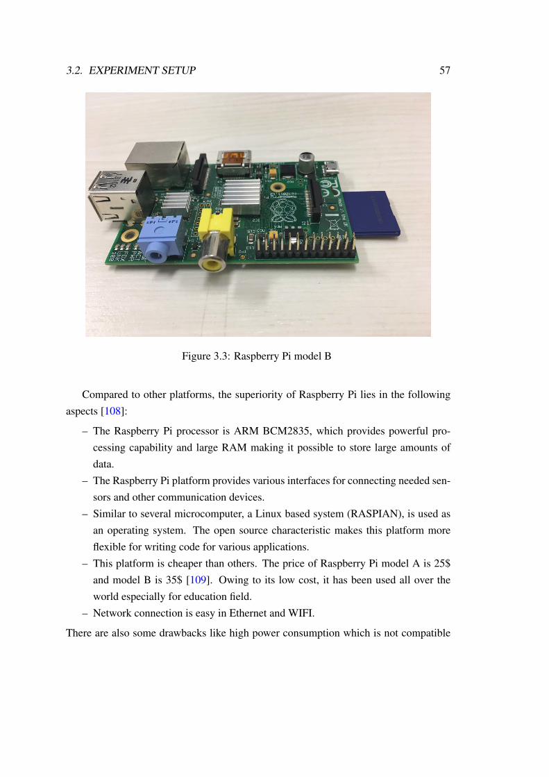
3.2. EXPERIMENT SETUP 57
Figure 3.3: Raspberry Pi model B
Compared to other platforms, the superiority of Raspberry Pi lies in the followingaspects [108]:
– The Raspberry Pi processor is ARM BCM2835, which provides powerful pro-cessing capability and large RAM making it possible to store large amounts ofdata.
– The Raspberry Pi platform provides various interfaces for connecting needed sen-sors and other communication devices.
– Similar to several microcomputer, a Linux based system (RASPIAN), is used asan operating system. The open source characteristic makes this platform moreflexible for writing code for various applications.
– This platform is cheaper than others. The price of Raspberry Pi model A is 25$and model B is 35$ [109]. Owing to its low cost, it has been used all over theworld especially for education field.
– Network connection is easy in Ethernet and WIFI.
There are also some drawbacks like high power consumption which is not compatible
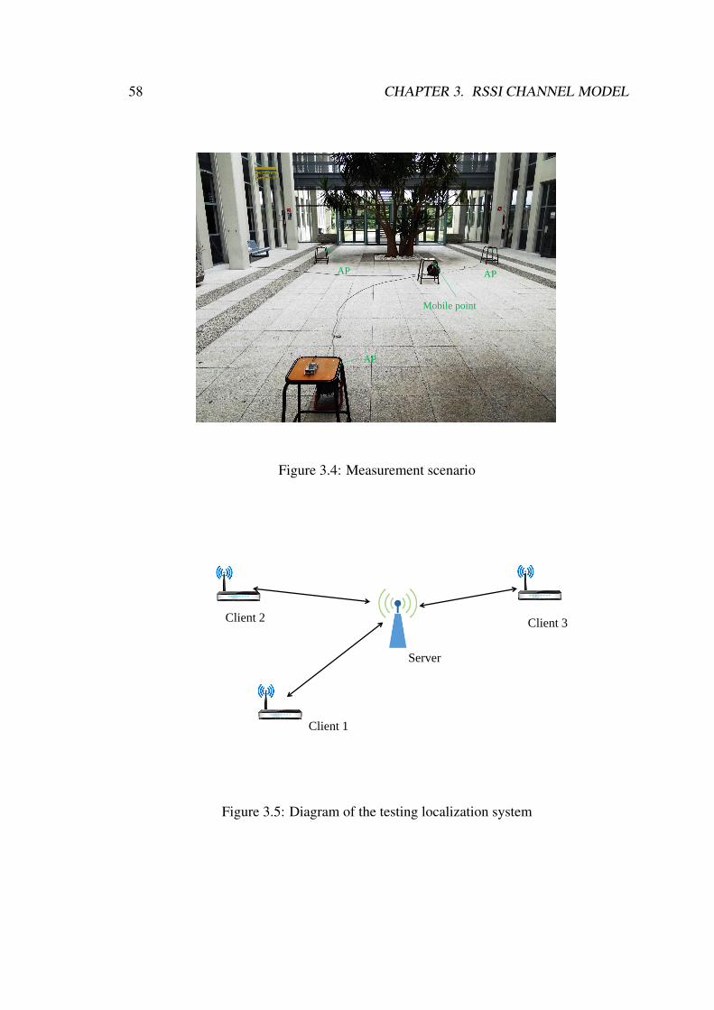
58 CHAPTER 3. RSSI CHANNEL MODEL
AP AP
Mobile point
AP
Figure 3.4: Measurement scenario
Server
Client 1
Client 3 Client 2
Figure 3.5: Diagram of the testing localization system

3.2. EXPERIMENT SETUP 59
with energy efficient sensor nodes.In our experiment, the Raspberry Pi is adopted to build the localization system.
Raspberry Pi model A is shown in Figure 3.2, which is configured as an access pointin our localization system and Raspberry Pi model B is shown in Figure 3.3, which isdefined as a mobile node. The experiment has been done in a large hall. The testingscene is shown in Figure 3.4. The experimental testbed has been build using three wifiaccess points (AP) and a mobile wifi point. The three wifi access points represent thethree anchor nodes and the mobile wifi point is considered as the unknown node.
Table 3.2: Convertion relationship between percentage value and dBm by Cisco(%) dBm (%) dBm (%) dBm (%) dBm (%) dBm0 -113 21 -91 42 -68 63 -44 84 -221 -112 22 -90 43 -67 64 -44 85 -202 -111 23 -89 44 -65 65 -43 86 -193 -110 24 -88 45 -64 66 -42 87 -184 -109 25 -87 46 -63 67 -42 88 -175 -108 26 -86 47 -62 68 -41 89 -166 -107 27 -85 48 -60 69 -40 90 -157 -106 28 -84 49 -59 70 -39 91 -148 -105 29 -83 50 -58 71 -38 92 -139 -104 30 -82 51 -56 72 -37 93 -1210 -103 31 -81 52 -55 73 -35 94 -1011 -102 32 -80 53 -53 74 -34 95 -1011 -101 33 -79 54 -52 75 -33 96 -1013 -99 34 -78 55 -50 76 -32 97 -1014 -98 35 -77 56 -50 77 -30 98 -1015 -97 36 -75 57 -49 78 -29 99 -1016 -96 37 -74 58 -48 79 -28 100 -1017 -95 38 -73 59 -48 80 -2718 -94 39 -72 60 -47 81 -2519 -93 40 -70 61 -46 82 -2420 -92 41 -69 62 -45 83 -23
The schematic diagram of the testing localization system is shown in Figure 3.5. Inthis diagram, the mobile point can be considered as a server and three access points canbe regarded as three clients.
The RSSI data acquisition process can be divided into the following procedures:(1) Server initialization: the server starts up and waits clients to join.
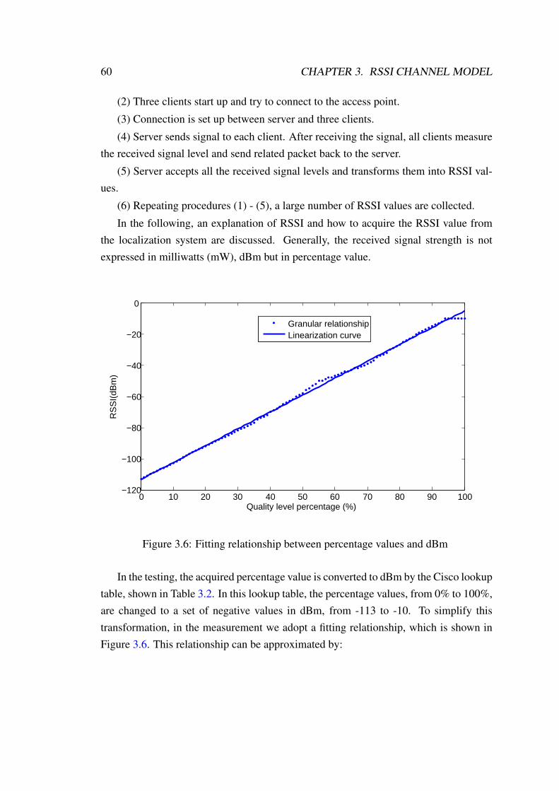
60 CHAPTER 3. RSSI CHANNEL MODEL
(2) Three clients start up and try to connect to the access point.
(3) Connection is set up between server and three clients.
(4) Server sends signal to each client. After receiving the signal, all clients measurethe received signal level and send related packet back to the server.
(5) Server accepts all the received signal levels and transforms them into RSSI val-ues.
(6) Repeating procedures (1) - (5), a large number of RSSI values are collected.
In the following, an explanation of RSSI and how to acquire the RSSI value fromthe localization system are discussed. Generally, the received signal strength is notexpressed in milliwatts (mW), dBm but in percentage value.
0 10 20 30 40 50 60 70 80 90 100−120
−100
−80
−60
−40
−20
0
Quality level percentage (%)
RS
SI(
dBm
)
Granular relationshipLinearization curve
Figure 3.6: Fitting relationship between percentage values and dBm
In the testing, the acquired percentage value is converted to dBm by the Cisco lookuptable, shown in Table 3.2. In this lookup table, the percentage values, from 0% to 100%,are changed to a set of negative values in dBm, from -113 to -10. To simplify thistransformation, in the measurement we adopt a fitting relationship, which is shown inFigure 3.6. This relationship can be approximated by:

3.3. EXPERIMENTAL CHANNEL MODEL 61
P (dBm) = 108.42percentage
100− 113.41 (3.5)
Table 3.3: Packet read from interface wlan0Interface Status link level noise
wlan0 0000 80 70% -256
To acquire RSSI values, we have created a python program to read the quality levelvalue. The data packets are illustrated in the Table 3.3. Among these data, the signallevel can be extracted and converted to values in dBm.
3.3 Experimental channel model
To characterize the RSSI model in an indoor environment, measurements have beenrealized. The experiment has been done in a large hall. The testing scene is shownin Figure 3.4. The experimental testbed has been build using three wifi access points(AP) and a mobile wifi device. To establish the practical channel model in this hall,many measurements have been performed on different positions. To acquire a largernumber of RSSI values, for each distance, the direction of the mobile point is changed30 times. Repeating this measurement process, a large number of RSSI data are obtainedby changing the distance from 1 meter to 10 meters with interval of 0.5 meters.
Based on the measured RSSI data, the median RSSI is calculated for one distance.Figure 3.7 presents the measured mean RSSI as function of the distance. As expected,we can find that the mean RSSI value decreases with the distance. From these resultswe can deduce the following channel model:
RSSIk = −9.40− 22.7log(dk) + vk (3.6)
with vk a zero-mean random variable with standard deviation σk. Therefore, based onthe measured data,Ak = −9.40, ηk = 2.27 can be deduced for the experimental channelmodel.
Meanwhile, the standard deviation of the noise for each distance can be estimated
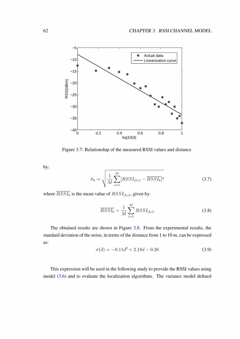
62 CHAPTER 3. RSSI CHANNEL MODEL
0 0.2 0.4 0.6 0.8 1−40
−35
−30
−25
−20
−15
−10
−5
log10(d)
RS
SI(
dBm
)
Actual dataLinearization curve
Figure 3.7: Relationship of the measured RSSI values and distance
by:
σk =
√√√√ 1
M
M∑i=1
[RSSI(k,i) −RSSIk]2 (3.7)
where RSSIk is the mean value of RSSI(k,i), given by:
RSSIk =1
M
M∑i=1
RSSI(k,i) (3.8)
The obtained results are shown in Figure 3.8. From the experimental results, thestandard deviation of the noise, in terms of the distance from 1 to 10 m, can be expressedas:
σ(d) = −0.11d2 + 2.18d− 0.38 (3.9)
This expression will be used in the following study to provide the RSSI values usingmodel (3.6) and to evaluate the localization algorithms. The variance model defined

3.3. EXPERIMENTAL CHANNEL MODEL 63
1 2 3 4 5 6 7 8 9 100
1
2
3
4
5
6
7
8
9
10
Distance (d)[m]
Sta
ndar
d de
viat
ion(
σ)
Measured dataApproximated curves
Figure 3.8: Relationship of the noise standard deviation and distance for measured data
by (3.9) is of course specific to our measurement condition but indicates that the RSSIvariance tends to increase with distance which has been already observed in some works[110]. It is worth noting that the relationship between the noise variance and distancedepends on the environment size and complexity.
Table 3.4: Environment information for four cases
Case Length(m) Width(m) Height(m)Obstaclenumber
Case1 15 8 5 0Case2 30 10 5.5 0Case3 15 8 5 2Case4 30 10 5.5 2
To confirm this trend, simulation is done using a ray tracing system for an environ-ment similar to the experimental environment. We have designed a ray tracing systemwhose simulation scenario is shown in Figure 3.9. As illustrated in this simulation sce-nario, there is a simulated workshop with two obstacles in it. A transmitter denoted byTX , sends signal to a mobile receiver denoted by RX , which moves from position 1

64 CHAPTER 3. RSSI CHANNEL MODEL
Figure 3.9: Simulation scenario of ray tracing system
to position 2. In the simulation, the median RSSI value is calculated based on thesesimulated data. The relationship between the distance and standard deviation of noisefor four cases are observed.
In this simulation, four cases are considered to observe different environment con-ditions. In the first two cases, we observe the relationship between the RSSI values anddistance with no obstacle in the room. In others cases, we change the room size or puttwo obstacles in it. The detailed information for these four cases is illustrated in Table3.4. In the simulation, for one position, 30 different RSSI values are measured and 180positions are considered by changing the distance from 1 meter to 10 meters with inter-val of 0.05 meters. Similarly, the median RSSI is calculated for one distance and therelationship between the distance and RSSI is plotted for four cases. These results areshown in Figure 3.10, Figure 3.11, Figure 3.12 and Figure 3.13.
Moreover, the linear approximation for the four cases is plotted in Figure 3.14.Based on these simulated RSSI data, the values of parameters A and η for all casesare estimated and given in Table 3.5.
From these results, we can compare the parameters for four cases. In the first and

3.3. EXPERIMENTAL CHANNEL MODEL 65
0 0.2 0.4 0.6 0.8 1−125
−120
−115
−110
−105
−100
log10(d)
RS
SI(
dBm
)
Simulated dataLinearization curve
Figure 3.10: Relationship of the simulated RSSI values and distance for case 1
0 0.2 0.4 0.6 0.8 1−125
−120
−115
−110
−105
−100
−95
log10(d)
RS
SI(
dBm
)
Simulated dataLinearization curve
Figure 3.11: Relationship of the simulated RSSI values and distance for case 2

66 CHAPTER 3. RSSI CHANNEL MODEL
0 0.2 0.4 0.6 0.8 1−130
−125
−120
−115
−110
−105
−100
−95
log10(d)
RS
SI(
dBm
)
Simulated dataLinearization curve
Figure 3.12: Relationship of the simulated RSSI values and distance for case 3
0 0.2 0.4 0.6 0.8 1−125
−120
−115
−110
−105
−100
−95
log10(d)
RS
SI(
dBm
)
Simulated dataLinearization curve
Figure 3.13: Relationship of the simulated RSSI values and distance for case 4

3.3. EXPERIMENTAL CHANNEL MODEL 67
0 0.1 0.2 0.3 0.4 0.5 0.6 0.7 0.8 0.9 1−120
−115
−110
−105
−100
−95
log10(d)
RS
SI(
dBm
)
Case 1Case 2Case 3Case 4
Figure 3.14: Comparison of the linearizion curves for four cases
Table 3.5: Different parameter values for four cases
Case A(dBm) η
Case1 -100.20 1.95Case2 -99.99 1.99Case3 -99.92 2.01Case4 -99.70 2.04
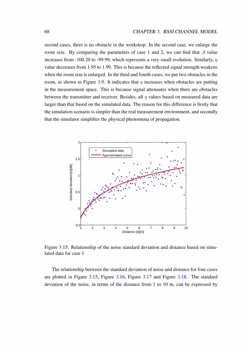
68 CHAPTER 3. RSSI CHANNEL MODEL
second cases, there is no obstacle in the workshop. In the second case, we enlarge theroom size. By comparing the parameters of case 1 and 2, we can find that A valueincreases from -100.20 to -99.99, which represents a very small evolution. Similarly, ηvalue decreases from 1.95 to 1.99. This is because the reflected signal strength weakenswhen the room size is enlarged. In the third and fourth cases, we put two obstacles in theroom, as shown in Figure 3.9. It indicates that η increases when obstacles are puttingin the measurement space. This is because signal attenuates when there are obstaclesbetween the transmitter and receiver. Besides, all η values based on measured data arelarger than that based on the simulated data. The reason for this difference is firstly thatthe simulation scenario is simpler than the real measurement environment, and secondlythat the simulator simplifies the physical phenomena of propagation.
1 2 3 4 5 6 7 8 9 10−0.5
0
0.5
1
1.5
2
Distance (d)[m]
Sta
ndar
d de
viat
ion(
σ)[d
B]
Simulated dataApproximated curve
Figure 3.15: Relationship of the noise standard deviation and distance based on simu-lated data for case 1
The relationship between the standard deviation of noise and distance for four casesare plotted in Figure 3.15, Figure 3.16, Figure 3.17 and Figure 3.18. The standarddeviation of the noise, in terms of the distance from 1 to 10 m, can be expressed by

3.3. EXPERIMENTAL CHANNEL MODEL 69
1 2 3 4 5 6 7 8 9 10−0.5
0
0.5
1
1.5
2
Distance (d)[m]
Sta
ndar
d de
viat
ion(
σ)[d
B]
Simulated dataApproximated curve
Figure 3.16: Relationship between the noise standard deviation and distance based onsimulated data for case 2
1 2 3 4 5 6 7 8 9 10−0.5
0
0.5
1
1.5
2
2.5
Distance (d)[m]
Sta
ndar
d de
viat
ion(
σ)[d
B]
Simulated dataApproximated curve
Figure 3.17: Relationship between the noise standard deviation and distance based onsimulated data for case 3
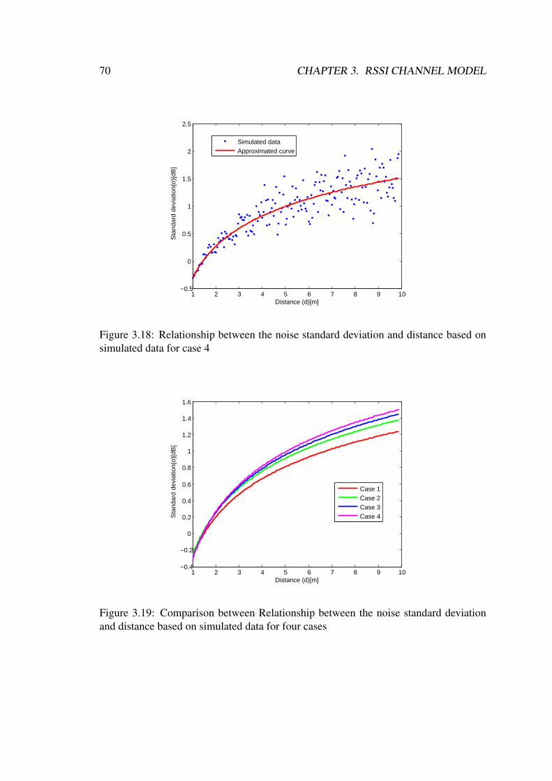
70 CHAPTER 3. RSSI CHANNEL MODEL
1 2 3 4 5 6 7 8 9 10−0.5
0
0.5
1
1.5
2
2.5
Distance (d)[m]
Sta
ndar
d de
viat
ion(
σ)[d
B]
Simulated dataApproximated curve
Figure 3.18: Relationship between the noise standard deviation and distance based onsimulated data for case 4
1 2 3 4 5 6 7 8 9 10−0.4
−0.2
0
0.2
0.4
0.6
0.8
1
1.2
1.4
1.6
Distance (d)[m]
Sta
ndar
d de
viat
ion(
σ)[d
B]
Case 1Case 2Case 3Case 4
Figure 3.19: Comparison between Relationship between the noise standard deviationand distance based on simulated data for four cases

3.4. CONCLUSION 71
(3.10) for case 1, (3.11) for case 2, (3.12) for case 3 and (3.13) for case 4 respectively.
σ(d) = −0.13d2 + 1.66d− 0.29 (3.10)
σ(d) = −0.13d2 + 1.78d− 0.27 (3.11)
σ(d) = −0.13d2 + 1.89d− 0.30 (3.12)
σ(d) = −0.15d2 + 1.96d− 0.31 (3.13)
From the above analysis on the simulated RSSI data, it can be observed that thereal and simulated data have a similar tendency in terms of the relationship betweenthe noise standard deviation and distance. The noise standard deviation increases withdistance. However, due to the complex environment, the standard deviation based onreal data is larger than the simulated data.
3.4 Conclusion
In this chapter, the lognormal shadowing path loss model which is employed as thetheoretical channel model for distance estimation has been introduced. In the experi-ment, the Raspberry Pi is adopted to build the localization system. The experiment hasbeen done in a large hall. To establish the practical channel model in this hall, manymeasurements have been performed on different positions. Based on the acquired RSSIdata, an experimental channel model has been constructed. To confirm this trend, simu-lation has done using a ray tracing system for an environment similar to the experimentalenvironment.
In the following chapter, three proposed localization algorithms: Three minimumDistances Method (TDM), Weighted Three minimum distances Method (WTM) andWeight values Adjustment Method (WAM) based on NLS and multilateration will bedeveloped. The comparison of TDM, WTM, WAM, LLS, NLS and POCS in terms ofthe localization accuracy and calculation time will be presented.


4Localization algorithms
The last chapter has shown that the relationship between the RSSI value and distancecan be written as:
RSSI(dBm) = A(dBm)− 10ηlog(d) + v (4.1)
where A and η are channel parameters whose values change with the environment andv is a noise whose variance is also largely variable. So the RSSI is not a reliable infor-mation to deduce the distance. The objective of this chapter is to propose and evaluatesome localization algorithms by taking into account the low accuracy of distances de-duced from RSSI measurements. Three approaches called three minimum distancesmethod (TDM), weighted three minimum distances method (WTM) and weight valuesadjustment method (WAM) are proposed. Using the testbed described in Chapter 3, ex-perimental channel model is deduced in order to verify the performance of the proposedalgorithms in realistic conditions. In the following parts, the proposed localization al-gorithms are detailed and performance comparison is presented.
73

74 CHAPTER 4. LOCALIZATION ALGORITHMS
4.1 Distance estimation from RSSI
All the proposed algorithms are based on the distance estimated from RSSI. So thefirst step of the study is to define a method to do this estimation and to evaluate thedistance accuracy.
Suppose that the distance estimation is based on M samples of RSSI(k,i), whichrepresents the ith RSSI sample measured by the kth anchor node.
For getting a good performance, the mean value of RSSI(k,i) is used to obtain thedistance estimate:
dk = 10Ak−RSSIk
10ηk (4.2)
where RSSIk, the mean RSSI value measured by the kth anchor, is given by:
RSSIk =1
M
M∑i=1
RSSI(k,i) (4.3)
It should be noticed that the mean value can be replaced by the median value inpractical situations with the advantage that the median value is less sensitive to outlets.In our model, because the RSSI(k,i) are Gaussian distributed, the mean value is equalto the median value.
Using channel model defined by (3.2) and substituting (4.3) to (4.2), we can deducethe estimated distance as:
dk = dk10− 1
10ηk
1M
M∑i=1
v(k,i)(4.4)
If the noise is small or the number of samples M is large, the estimated dk can beapproximated by:
dk ' dk[1−ln10
10ηk
1
M
M∑i=1
v(k,i)] (4.5)
Then the measurement error can be evaluated by the following additive noise:
ne = −dkln10
10ηk
1
M
M∑i=1
v(k,i) (4.6)
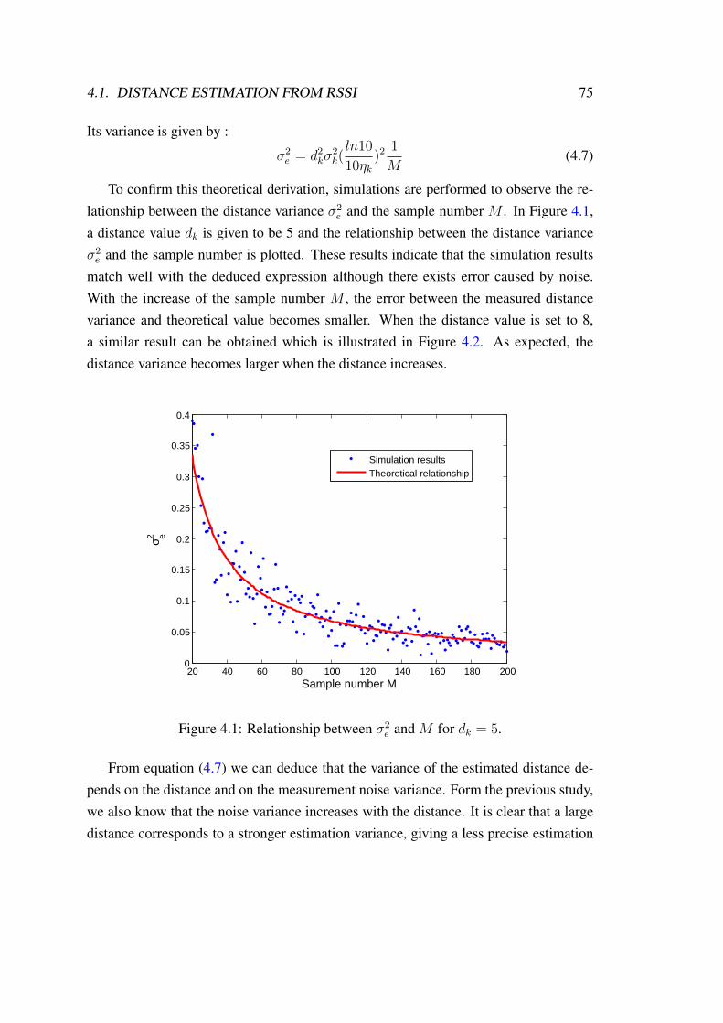
4.1. DISTANCE ESTIMATION FROM RSSI 75
Its variance is given by :
σ2e = d2kσ
2k(ln10
10ηk)2
1
M(4.7)
To confirm this theoretical derivation, simulations are performed to observe the re-lationship between the distance variance σ2
e and the sample number M . In Figure 4.1,a distance value dk is given to be 5 and the relationship between the distance varianceσ2e and the sample number is plotted. These results indicate that the simulation results
match well with the deduced expression although there exists error caused by noise.With the increase of the sample number M , the error between the measured distancevariance and theoretical value becomes smaller. When the distance value is set to 8,a similar result can be obtained which is illustrated in Figure 4.2. As expected, thedistance variance becomes larger when the distance increases.
20 40 60 80 100 120 140 160 180 2000
0.05
0.1
0.15
0.2
0.25
0.3
0.35
0.4
Sample number M
σe2
Simulation resultsTheoretical relationship
Figure 4.1: Relationship between σ2e and M for dk = 5.
From equation (4.7) we can deduce that the variance of the estimated distance de-pends on the distance and on the measurement noise variance. Form the previous study,we also know that the noise variance increases with the distance. It is clear that a largedistance corresponds to a stronger estimation variance, giving a less precise estimation

76 CHAPTER 4. LOCALIZATION ALGORITHMS
20 40 60 80 100 120 140 160 180 2000
0.2
0.4
0.6
0.8
1
1.2
1.4
Sample number M
σe2
Simulation resultsTheoretical relationship
Figure 4.2: Relationship between σ2e and M for dk = 8.
of the distance. Expression (4.7) provides some guidances to reduce the localizationerror, such as using the smallest distance from the unknown node to anchor nodes orincreasing the sample number M . Another strategy is to exploit this property in the def-inition of the localization algorithms, which will be described in the following sections.
4.2 Localization methods
4.2.1 Multilateration
The multilateration algorithm is a basic positioning method, widely used in manylocalization systems [111]. In this algorithm, at least three anchor nodes are needed fortwo dimension localization. The position of the anchor nodes is assumed to be known.The relationship between the unknown node position and N anchor nodes positions can
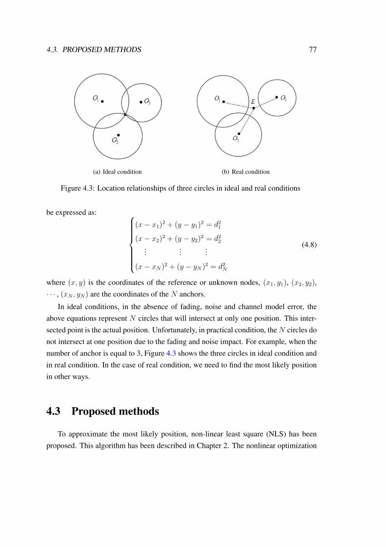
4.3. PROPOSED METHODS 77
(a) Ideal condition (b) Real condition
Figure 4.3: Location relationships of three circles in ideal and real conditions
be expressed as:
(x− x1)2 + (y − y1)2 = d21
(x− x2)2 + (y − y2)2 = d22...
......
(x− xN)2 + (y − yN)2 = d2N
(4.8)
where (x, y) is the coordinates of the reference or unknown nodes, (x1, y1), (x2, y2),· · · , (xN , yN) are the coordinates of the N anchors.
In ideal conditions, in the absence of fading, noise and channel model error, theabove equations represent N circles that will intersect at only one position. This inter-sected point is the actual position. Unfortunately, in practical condition, theN circles donot intersect at one position due to the fading and noise impact. For example, when thenumber of anchor is equal to 3, Figure 4.3 shows the three circles in ideal condition andin real condition. In the case of real condition, we need to find the most likely positionin other ways.
4.3 Proposed methods
To approximate the most likely position, non-linear least square (NLS) has beenproposed. This algorithm has been described in Chapter 2. The nonlinear optimization
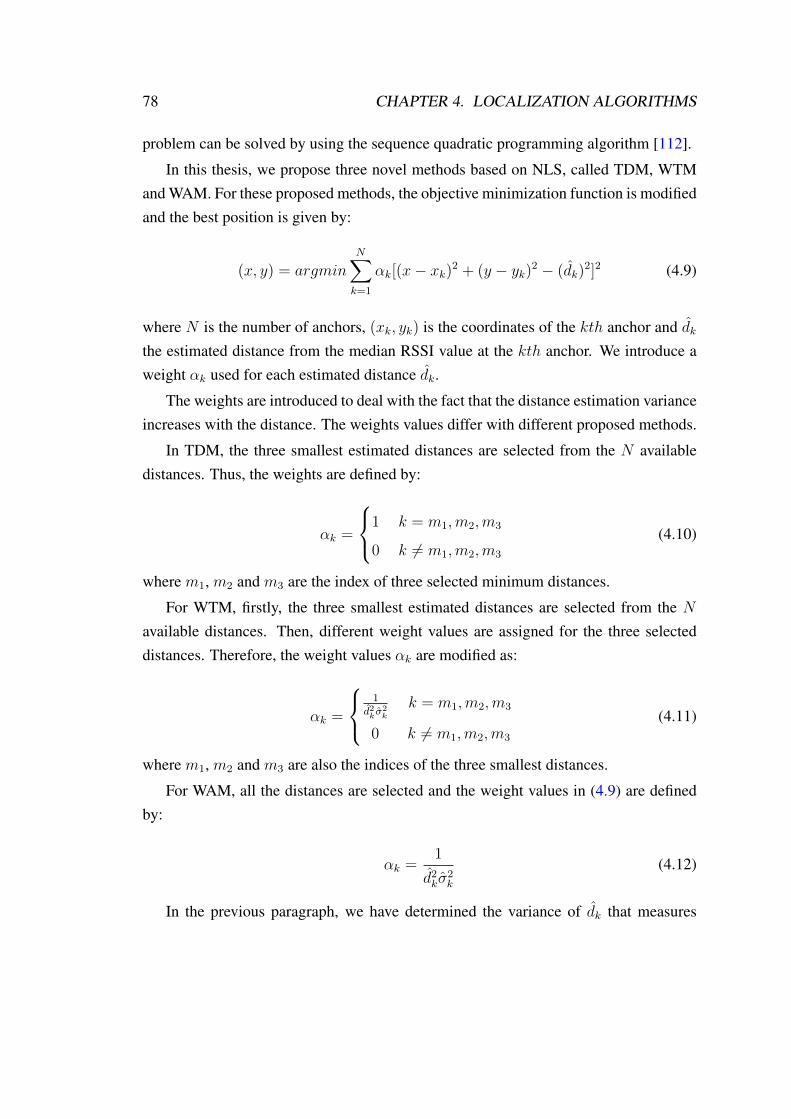
78 CHAPTER 4. LOCALIZATION ALGORITHMS
problem can be solved by using the sequence quadratic programming algorithm [112].
In this thesis, we propose three novel methods based on NLS, called TDM, WTMand WAM. For these proposed methods, the objective minimization function is modifiedand the best position is given by:
(x, y) = argminN∑k=1
αk[(x− xk)2 + (y − yk)2 − (dk)2]2 (4.9)
where N is the number of anchors, (xk, yk) is the coordinates of the kth anchor and dkthe estimated distance from the median RSSI value at the kth anchor. We introduce aweight αk used for each estimated distance dk.
The weights are introduced to deal with the fact that the distance estimation varianceincreases with the distance. The weights values differ with different proposed methods.
In TDM, the three smallest estimated distances are selected from the N availabledistances. Thus, the weights are defined by:
αk =
1 k = m1,m2,m3
0 k 6= m1,m2,m3
(4.10)
where m1, m2 and m3 are the index of three selected minimum distances.
For WTM, firstly, the three smallest estimated distances are selected from the Navailable distances. Then, different weight values are assigned for the three selecteddistances. Therefore, the weight values αk are modified as:
αk =
1
d2kσ2k
k = m1,m2,m3
0 k 6= m1,m2,m3
(4.11)
where m1, m2 and m3 are also the indices of the three smallest distances.
For WAM, all the distances are selected and the weight values in (4.9) are definedby:
αk =1
d2kσ2k
(4.12)
In the previous paragraph, we have determined the variance of dk that measures

4.4. SIMULATION AND LOCALIZATION PERFORMANCE 79
the dispersion of the estimated distance around the true distance. The values of theweights are chosen to be proportional to the inverse of this variance in (4.7). Hence,the uncertainty of the measured distances can be taken into account in the objectivefunction.
The six different methods based on multilateration: TDM, WTM, WAM, LLS, NLSand POCS will be evaluated in the following section. Furthermore, the accuracy andcalculation time of these six methods will be compared.
4.4 Simulation and localization performance
Figure 4.4: Grid defining the intersection positions and anchor nodes positions
After acquiring the channel model from the experimental data, the whole localiza-tion process can be evaluated in a given region. As shown in Figure 4.4, eight anchornodes are set in the predefined positions with coordinates A(0, 6), B(0, 0), C(6, 0),D(6, 6), E(0, 3), F (3, 0), G(6, 3), H(3, 6). In the coordinate scale, 1 denotes 1 meter.When the number of anchors is three, the anchor nodes are located at A, B, and C.
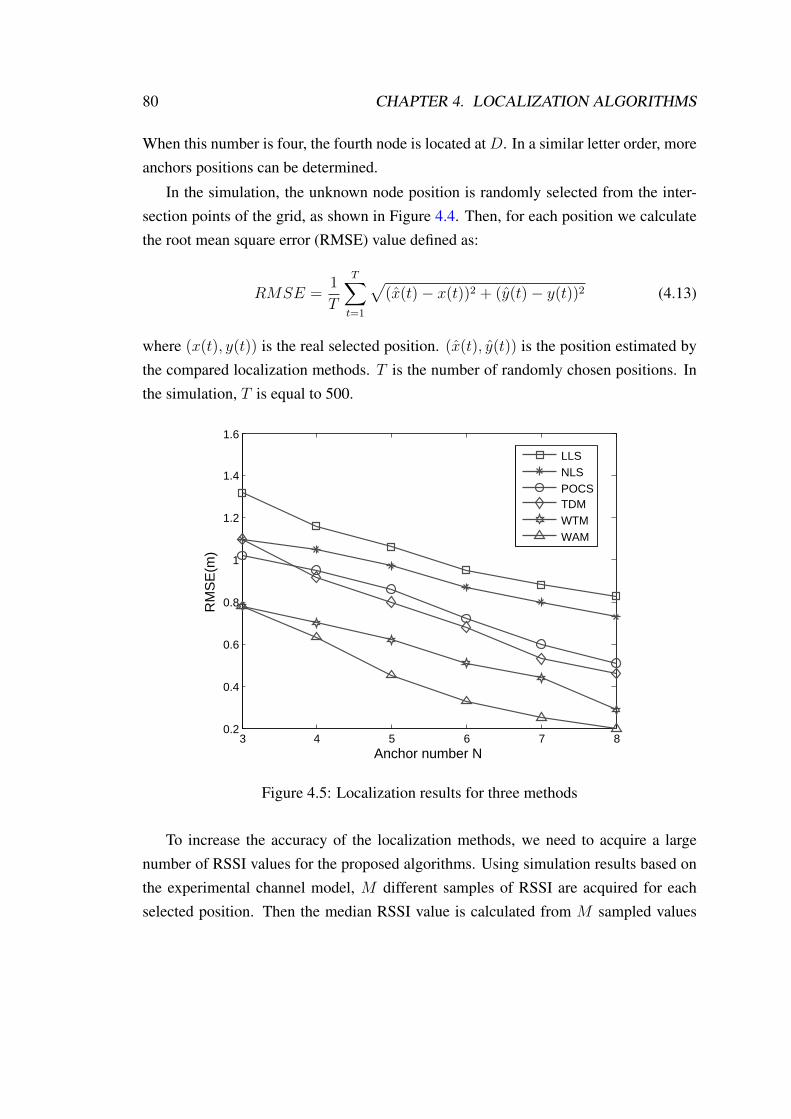
80 CHAPTER 4. LOCALIZATION ALGORITHMS
When this number is four, the fourth node is located at D. In a similar letter order, moreanchors positions can be determined.
In the simulation, the unknown node position is randomly selected from the inter-section points of the grid, as shown in Figure 4.4. Then, for each position we calculatethe root mean square error (RMSE) value defined as:
RMSE =1
T
T∑t=1
√(x(t)− x(t))2 + (y(t)− y(t))2 (4.13)
where (x(t), y(t)) is the real selected position. (x(t), y(t)) is the position estimated bythe compared localization methods. T is the number of randomly chosen positions. Inthe simulation, T is equal to 500.
3 4 5 6 7 80.2
0.4
0.6
0.8
1
1.2
1.4
1.6
Anchor number N
RM
SE
(m)
LLSNLSPOCSTDMWTMWAM
Figure 4.5: Localization results for three methods
To increase the accuracy of the localization methods, we need to acquire a largenumber of RSSI values for the proposed algorithms. Using simulation results based onthe experimental channel model, M different samples of RSSI are acquired for eachselected position. Then the median RSSI value is calculated from M sampled values
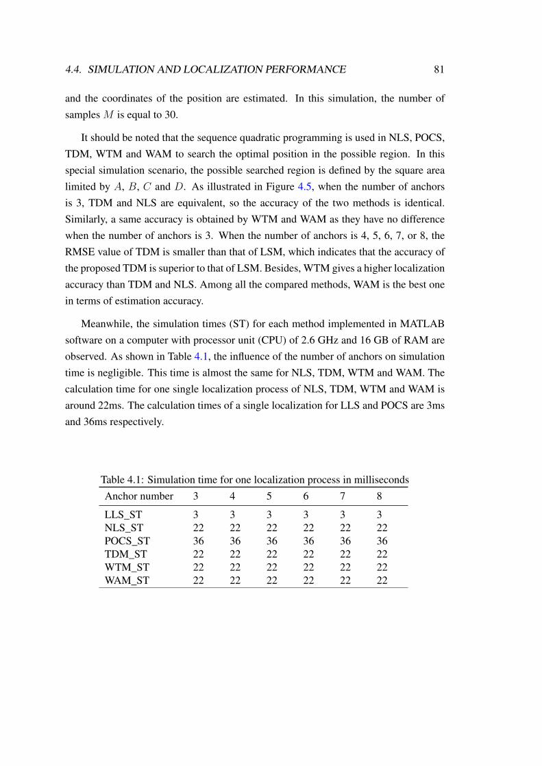
4.4. SIMULATION AND LOCALIZATION PERFORMANCE 81
and the coordinates of the position are estimated. In this simulation, the number ofsamples M is equal to 30.
It should be noted that the sequence quadratic programming is used in NLS, POCS,TDM, WTM and WAM to search the optimal position in the possible region. In thisspecial simulation scenario, the possible searched region is defined by the square arealimited by A, B, C and D. As illustrated in Figure 4.5, when the number of anchorsis 3, TDM and NLS are equivalent, so the accuracy of the two methods is identical.Similarly, a same accuracy is obtained by WTM and WAM as they have no differencewhen the number of anchors is 3. When the number of anchors is 4, 5, 6, 7, or 8, theRMSE value of TDM is smaller than that of LSM, which indicates that the accuracy ofthe proposed TDM is superior to that of LSM. Besides, WTM gives a higher localizationaccuracy than TDM and NLS. Among all the compared methods, WAM is the best onein terms of estimation accuracy.
Meanwhile, the simulation times (ST) for each method implemented in MATLABsoftware on a computer with processor unit (CPU) of 2.6 GHz and 16 GB of RAM areobserved. As shown in Table 4.1, the influence of the number of anchors on simulationtime is negligible. This time is almost the same for NLS, TDM, WTM and WAM. Thecalculation time for one single localization process of NLS, TDM, WTM and WAM isaround 22ms. The calculation times of a single localization for LLS and POCS are 3msand 36ms respectively.
Table 4.1: Simulation time for one localization process in millisecondsAnchor number 3 4 5 6 7 8
LLS_ST 3 3 3 3 3 3NLS_ST 22 22 22 22 22 22POCS_ST 36 36 36 36 36 36TDM_ST 22 22 22 22 22 22WTM_ST 22 22 22 22 22 22WAM_ST 22 22 22 22 22 22

82 CHAPTER 4. LOCALIZATION ALGORITHMS
4.5 Conclusion
In this chapter, three proposed localization algorithms: Three minimum DistancesMethod (TDM), Weighted Three minimum distances Method (WTM) and Weight val-ues Adjustment Method (WAM) based on NLS and multilateration have been described.For getting a good performance, the median RSSI value is used to obtain the distanceestimate. Multilateration is adopted in the position process. The comparison of TDM,WTM, WAM, LLS, NLS and POCS in terms of localization accuracy and calculationtime has been presented.
In this chapter, we have assumed that the channel parameters (A and η) are perfectlyknown. The error in distance estimation is due to the noise v. In a real application, theseparameters will change with time. Therefore, it is necessary to learn these parameters.In the next chapter, we will develop methods to acquire and track the evolution of thechannel model.

5Tracking strategy
In our work, we consider the localization of the target when the environment changesfrequently and RSSI channel model parameters have variation. Different from the ex-isting channel model based algorithms, we reduce the localization error caused fromparameter variation by a grid based learning and tracking strategy. In the context ofapplications where the positions are constrained on a grid, a novel tracking strategy isproposed to determine the real position and obtain the actual parameters in the moni-tored region. Based on practical data acquired from the testbed described in Chapter3, an experimental channel model is constructed to provide RSSI values and verify theproposed tracking strategy. The simulation results show a good behavior of the pro-posed tracking strategy in presence of space-time variation of the propagation channel.Compared with the existing RSSI based algorithms, the proposed tracking strategy ex-hibits better localization accuracy but consumes more calculation time. In addition, atracking test is performed to validate the effectiveness of the proposed tracking strategy.
In the next sections, the proposed parameter tracking strategy and localization algo-rithm will be described. Localization and tracking results for assessing the performanceof the proposed technique and analyzing its limitation will be provided. Furthermore,the localization performance comparison and tracking test will be presented.
83
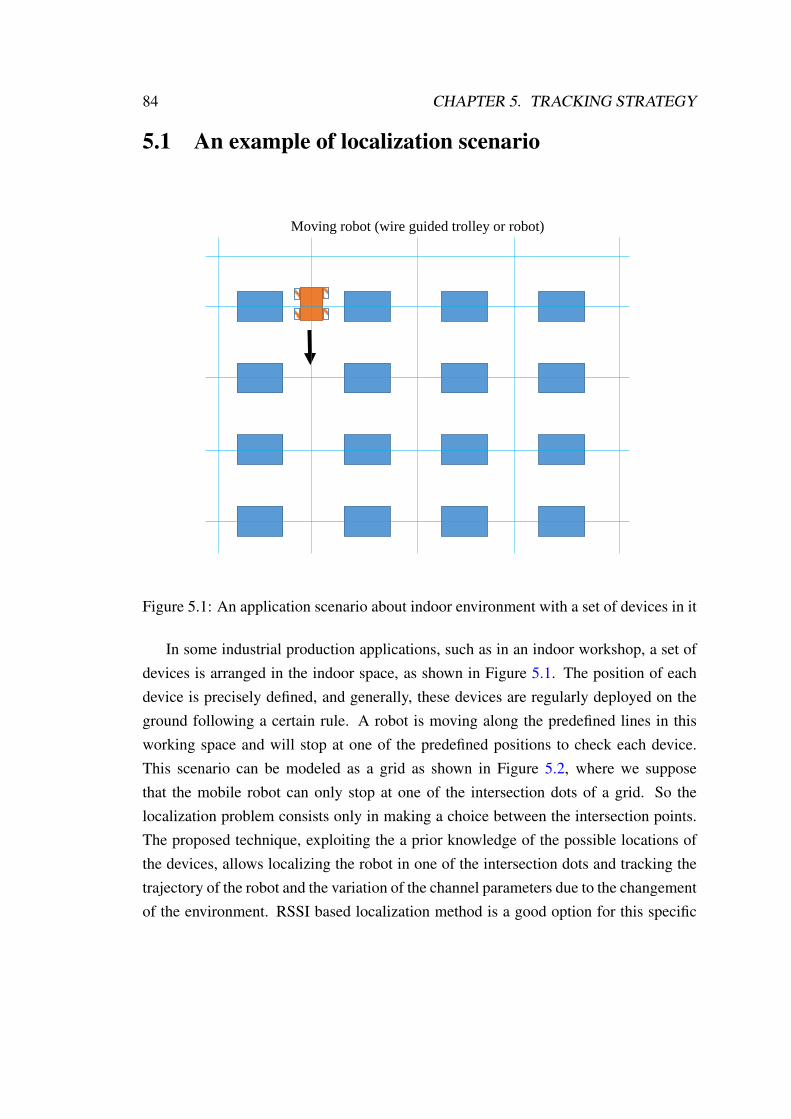
84 CHAPTER 5. TRACKING STRATEGY
5.1 An example of localization scenario
Moving robot (wire guided trolley or robot)
Figure 5.1: An application scenario about indoor environment with a set of devices in it
In some industrial production applications, such as in an indoor workshop, a set ofdevices is arranged in the indoor space, as shown in Figure 5.1. The position of eachdevice is precisely defined, and generally, these devices are regularly deployed on theground following a certain rule. A robot is moving along the predefined lines in thisworking space and will stop at one of the predefined positions to check each device.This scenario can be modeled as a grid as shown in Figure 5.2, where we supposethat the mobile robot can only stop at one of the intersection dots of a grid. So thelocalization problem consists only in making a choice between the intersection points.The proposed technique, exploiting the a prior knowledge of the possible locations ofthe devices, allows localizing the robot in one of the intersection dots and tracking thetrajectory of the robot and the variation of the channel parameters due to the changementof the environment. RSSI based localization method is a good option for this specific

5.1. AN EXAMPLE OF LOCALIZATION SCENARIO 85
application but we have to check that
(1) errors due to the channel model inaccuracy are less than the grid resolution,
(2) small position error correction is possible and can be used to track in real timethe channel variations.
These two conditions will be developed later in the following section. Without lossof generality, we consider in this study that the size of the grid is 10m× 10m. Anchorsare placed on three dots, whose coordinates are (0, 0), (0, 10), (10, 0), respectively. Inthe coordinate scale, 1 denotes 1 meter. There exists a reference node in the center ofthis region, whose position is (5, 5).
D
G
A
10
y
x
0
1
1
2
3
5
6
4
2
3
5
4
6
0
1
2
3
4
5
6
7
8
9
10
1
2
3
4
5
6
7
8
9
B
C
E
H
F
Figure 5.2: Grid defining the possible positions
86 CHAPTER 5. TRACKING STRATEGY
5.2 Distance estimation
Suppose that the distance estimation is based on M samples of RSSI(k,i), whichrepresents the ith RSSI sample measured by the kth anchor node. For getting a goodperformance, the median value of RSSI(k,i) is used to obtain the distance estimate:
dk = 10Ak−RSSIk
10ηk (5.1)
where RSSIk, the median RSSI value measured by the kth anchor, is given by:
RSSIk = Median{RSSI(k,i), i = 1, · · · ,M} (5.2)
5.3 Trilateration algorithm
In Chapter 2, many positioning methods have been described. Compared to otheroptimization methods, trilateration algorithm can compute the position directly andquickly on condition that three anchors are non-linearly placed. Therefore, in the pro-posed tracking strategy, to reduce the calculation time, the trilateration algorithm isemployed to calculate the position. The trilateration algorithm is a basic positioningmethod, widely used in many localization systems [113]. In this algorithm, at leastthree anchor nodes are needed for positioning the target. The position of the anchornodes is assumed to be known. As presented in Chapter 2, the relationship between theunknown node position and three anchor node positions can be expressed as [114]:
(x− x1)2 + (y − y1)2 + (z − z1)2 = d21
(x− x2)2 + (y − y2)2 + (z − z2)2 = d22
(x− x3)2 + (y − y3)2 + (z − z3)2 = d23
(5.3)
where (x, y, z) are the coordinates of the reference or unknown node, (x1, y1, z1), (x2, y2, z2),(x3, y3, z3) are the coordinates of the three anchors. Equations (5.3) can be written intothe following matrix form:
Qx = b (5.4)
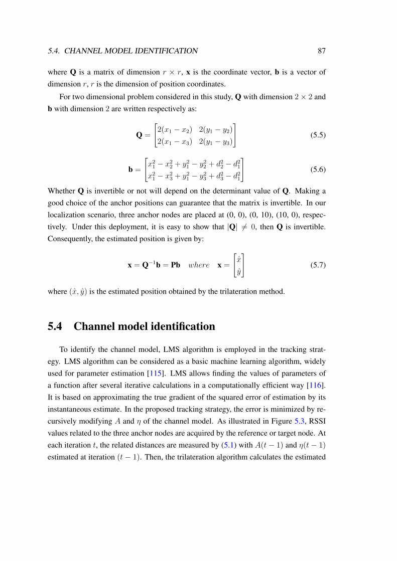
5.4. CHANNEL MODEL IDENTIFICATION 87
where Q is a matrix of dimension r × r, x is the coordinate vector, b is a vector ofdimension r, r is the dimension of position coordinates.
For two dimensional problem considered in this study, Q with dimension 2× 2 andb with dimension 2 are written respectively as:
Q =
[2(x1 − x2) 2(y1 − y2)2(x1 − x3) 2(y1 − y3)
](5.5)
b =
[x21 − x22 + y21 − y22 + d22 − d21x21 − x23 + y21 − y23 + d23 − d21
](5.6)
Whether Q is invertible or not will depend on the determinant value of Q. Making agood choice of the anchor positions can guarantee that the matrix is invertible. In ourlocalization scenario, three anchor nodes are placed at (0, 0), (0, 10), (10, 0), respec-tively. Under this deployment, it is easy to show that |Q| 6= 0, then Q is invertible.Consequently, the estimated position is given by:
x = Q−1b = Pb where x =
[x
y
](5.7)
where (x, y) is the estimated position obtained by the trilateration method.
5.4 Channel model identification
To identify the channel model, LMS algorithm is employed in the tracking strat-egy. LMS algorithm can be considered as a basic machine learning algorithm, widelyused for parameter estimation [115]. LMS allows finding the values of parameters ofa function after several iterative calculations in a computationally efficient way [116].It is based on approximating the true gradient of the squared error of estimation by itsinstantaneous estimate. In the proposed tracking strategy, the error is minimized by re-cursively modifying A and η of the channel model. As illustrated in Figure 5.3, RSSIvalues related to the three anchor nodes are acquired by the reference or target node. Ateach iteration t, the related distances are measured by (5.1) with A(t− 1) and η(t− 1)
estimated at iteration (t − 1). Then, the trilateration algorithm calculates the estimated

88 CHAPTER 5. TRACKING STRATEGY
position (x(t), y(t)). With the known real position of reference point (x, y), the local-ization error is formulated as:
ε(t) =√
(x(t)− x(t))2 + (y(t)− y(t))2 (5.8)
where t denotes the iteration number.
This error serves as the input to the LMS algorithm, by adaptively minimizing thelocalization error, we obtain η as follows:
η(t) = η(t− 1)− µη∂ε(t)2
∂η(5.9)
The derivative of ε(t)2 with respect to η is:
∂ε(t)2
∂η=∂[(x(t)− x(t))2 + (y(t)− y(t))2]
∂η
= 2[x(t)− x(t)]∂x(t)
∂η+ 2[y(t)− y(t)]
∂y(t)
∂η
(5.10)
The derivatives of the estimated position x(t) and y(t) with respect to η are given by:
∂x(t)
∂η= −2P(1, 1)d1
∂d1∂η
+ 2P(1, 1)d2∂d2∂η
−2P(1, 2)d1∂d1∂η
+ 2P(1, 2)d3∂d3∂η
(5.11)
∂y(t)
∂η= −2P(2, 1)d1
∂d1∂η
+ 2P(2, 1)d2∂d2∂η
−2P(2, 2)d1∂d1∂η
+ 2P(2, 2)d3∂d3∂η
(5.12)
∂dk∂η
= −ln(10)10A−RSSIk
10ηA−RSSIk
10
1
η2(5.13)
Similarly, we can get A from the following equation:
A(t) = A(t− 1)− µA∂ε(t)2
∂A(5.14)

5.5. TRACKING STRATEGY 89
The derivative of ε(t)2 with respect to A is:
∂ε(t)2
∂A=∂[(x(t)− x(t))2 + (y(t)− y(t))2]
∂A
= 2[x(t)− x(t)]∂x(t)
∂A+ 2[y(t)− y(t)]
∂y(t)
∂A
(5.15)
The derivatives of the estimated position x(t) and y(t) with respect to A are givenby:
∂x(t)
∂A= −2P(1, 1)d1
∂d1∂A
+ 2P(1, 1)d2∂d2∂A
−2P(1, 2)d1∂d1∂A
+ 2P(1, 2)d3∂d3∂A
(5.16)
∂y(t)
∂A= −2P(2, 1)d1
∂d1∂A
+ 2P(2, 1)d2∂d2∂A
−2P(2, 2)d1∂d1∂A
+ 2P(2, 2)d3∂d3∂A
(5.17)
∂dk∂A
= ln(10)10A−RSSIk
10η1
10η(5.18)
where µη and µA are the adaptation step size, which can be adjusted experimentally.
5.5 Tracking strategy
The whole proposed tracking strategy and localization process are illustrated in Fig-ure 5.3. In the proposed algorithm, this task is done in two steps: an initial channelestimation using a reference node followed by a tracking procedure using a grid correc-tion based on the constrained positions.
In the first step, the mobile robot is positioned at a reference point whose positionis known. Then the trilateration algorithm is used to estimate the location and LMS isemployed to find the channel parameters A and η which minimize the positioning error.
After the acquisition step, a grid correction strategy is adopted for the localizationand channel variation tracking. We subdivide this step into the following procedures.
1. Based on A and η obtained in the acquisition step, we estimate the unknown nodeposition denoted by (x, y).

90 CHAPTER 5. TRACKING STRATEGY
2. After getting (x, y), we calculate all the distance values between (x, y) and theintersection points in the grid. The nearest intersection point will be selected as the mostlikely position, whose coordinates are (x, y).
3. Knowing the most likely position (x, y), we use LMS to track the space and timeevolution of the channel parameters, the tracked parameters are denoted by A and η.
4. These procedures can be repeated in real time.The process can be easily extended to a scenario where there are also non-anchor
nodes in fixed positions that first localize themselves and then contribute to the tracking.
Figure 5.3: Diagram of tracking principle
5.6 Localization results
After acquiring the channel model from the experimental data, we can evaluate thelocalization process using simulation. As shown in Figure 5.2, we set three anchornodes in the three predefined positions with coordinates A(0, 10), B(0, 0), C(10, 0),respectively. In the simulation, the unknown node position is randomly selected fromthe intersection points of the grid. Then, for each position we calculate the RMSE valuedefined as [117]:
RMSE =1
T
T∑t=1
√(x(t)− x(t))2 + (y(t)− y(t))2 (5.19)
where (x(t), y(t)) is the actual selected position. (x(t), y(t)) is the position estimatedby the trilateration method. T is the number of randomly chosen positions. In the

5.7. PARAMETER CONVERGENCE 91
simulation, T is equal to 500.
Table 5.1: Localization accuracySample number M 30 50 200 300 500 1000
RMSE (m) 0.78 0.56 0.33 0.25 0.14 0.10
As illustrated in Table 5.1, with the increase of sample numberM , the RMSE valuesof localization algorithm decrease, which indicates that the accuracy of localization getsbetter. To guarantee the efficiency of the tracking strategy, in the following tracking stepand simulations, the sample number M is set to 300.
5.7 Parameter convergence
0 50 100 150 200 250 300 350 400 4502.18
2.2
2.22
2.24
2.26
2.28
2.3
N(localization times)
η
Figure 5.4: Convergence process of η.
In the acquisition step, the actual values of A and η are −10dBm and 2.24 respec-tively, and the initial values are −9dBm and 2.28. As illustrated in Figure 5.4 andFigure 5.5, after the acquisition step, with the help of trilateration and LMS methods,

92 CHAPTER 5. TRACKING STRATEGY
0 50 100 150 200 250 300 350 400 450−11.5
−11
−10.5
−10
−9.5
−9
N(localization times)
A(d
Bm
)
Figure 5.5: Convergence process of A
we can obtain A value very close to −10dBm. Similarly, the obtained η value is veryclose to 2.24. Furthermore, in the tracking step, we suppose that the true value of A is−11dBm and the true value of η is 2.20. In the same manner, we can get A value veryclose to −11dBm and η value very close to 2.20. So, the proposed strategy can trackthe variation of the parameters in the monitored region.
5.8 Limitation analysis
However, there exists a limitation in the grid correction. If the localization error islarger than the grid step size, it is no more guaranteed that the correction strategy willbe efficient. Therefore, we need to analyse the relationship between the step size andparameter variation which gives us a criterion to choose an appropriate step size value.The localization error is defined as [118]:
ε(t) =√
(x(t)− x(t))2 + (y(t)− y(t))2 (5.20)
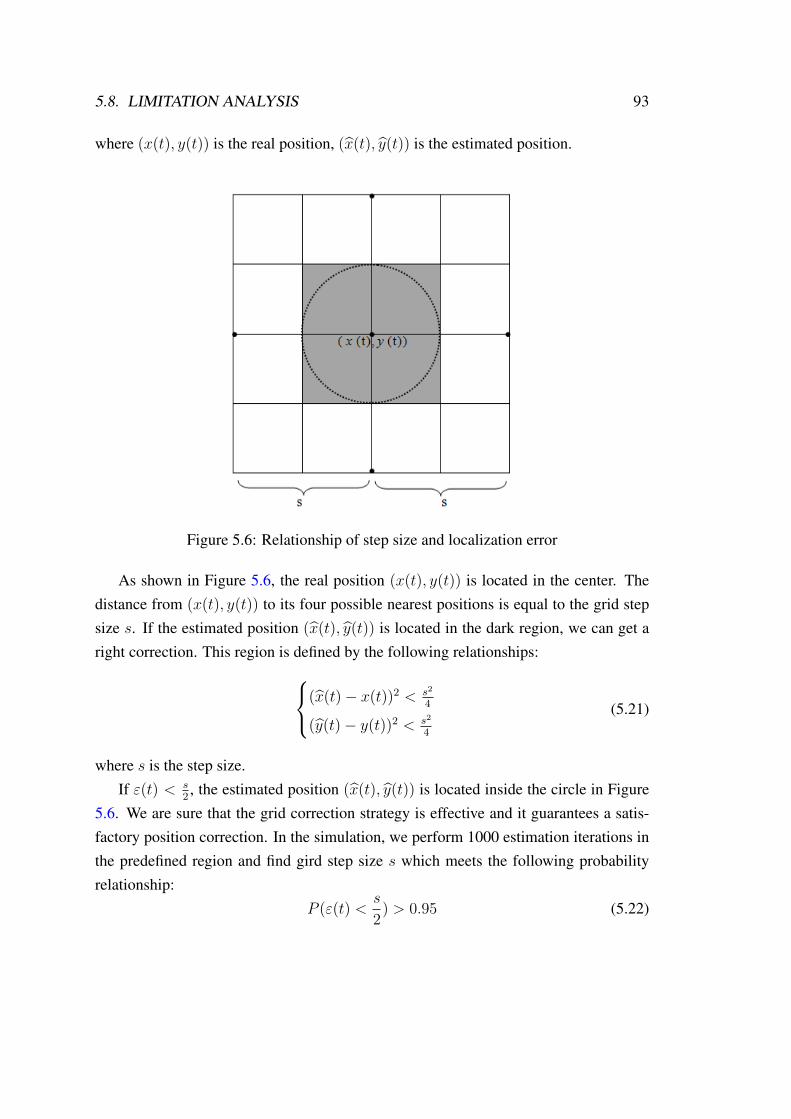
5.8. LIMITATION ANALYSIS 93
where (x(t), y(t)) is the real position, (x(t), y(t)) is the estimated position.
Figure 5.6: Relationship of step size and localization error
As shown in Figure 5.6, the real position (x(t), y(t)) is located in the center. Thedistance from (x(t), y(t)) to its four possible nearest positions is equal to the grid stepsize s. If the estimated position (x(t), y(t)) is located in the dark region, we can get aright correction. This region is defined by the following relationships:(x(t)− x(t))2 < s2
4
(y(t)− y(t))2 < s2
4
(5.21)
where s is the step size.If ε(t) < s
2, the estimated position (x(t), y(t)) is located inside the circle in Figure
5.6. We are sure that the grid correction strategy is effective and it guarantees a satis-factory position correction. In the simulation, we perform 1000 estimation iterations inthe predefined region and find gird step size s which meets the following probabilityrelationship:
P (ε(t) <s
2) > 0.95 (5.22)
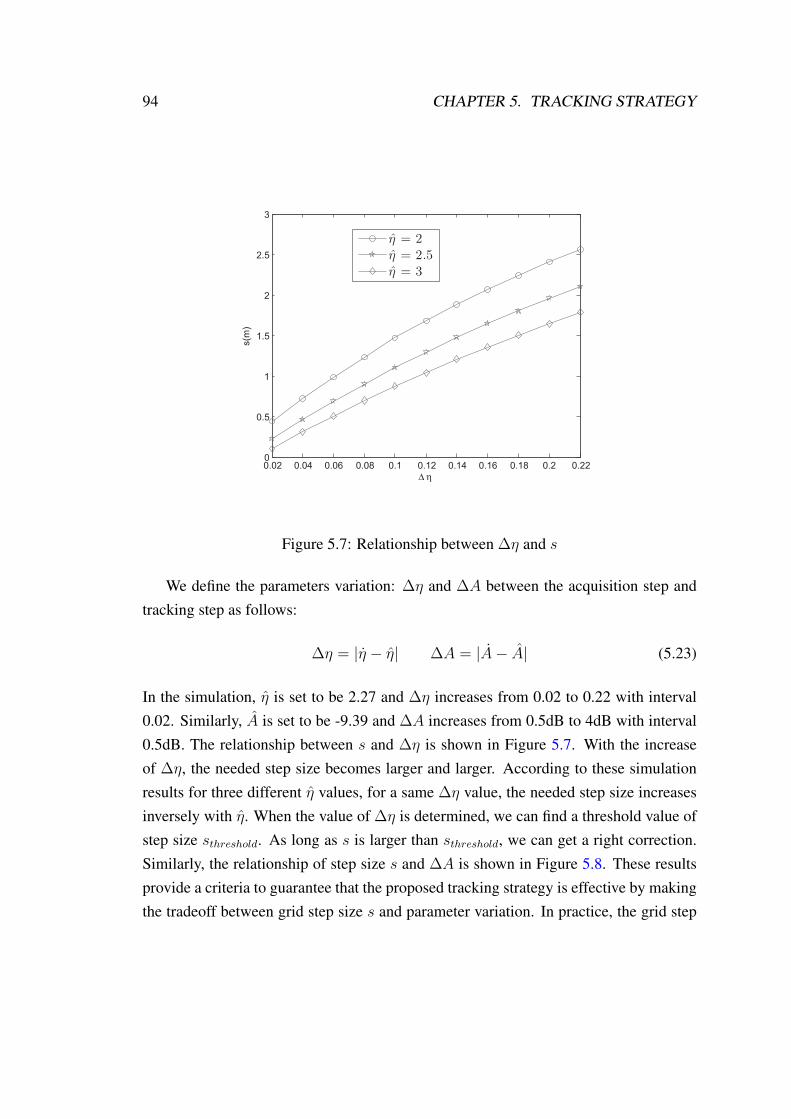
94 CHAPTER 5. TRACKING STRATEGY
0.02 0.04 0.06 0.08 0.1 0.12 0.14 0.16 0.18 0.2 0.220
0.5
1
1.5
2
2.5
3
Δ η
s(m
)η = 2
η = 2.5
η = 3
Figure 5.7: Relationship between ∆η and s
We define the parameters variation: ∆η and ∆A between the acquisition step andtracking step as follows:
∆η = |η − η| ∆A = |A− A| (5.23)
In the simulation, η is set to be 2.27 and ∆η increases from 0.02 to 0.22 with interval0.02. Similarly, A is set to be -9.39 and ∆A increases from 0.5dB to 4dB with interval0.5dB. The relationship between s and ∆η is shown in Figure 5.7. With the increaseof ∆η, the needed step size becomes larger and larger. According to these simulationresults for three different η values, for a same ∆η value, the needed step size increasesinversely with η. When the value of ∆η is determined, we can find a threshold value ofstep size sthreshold. As long as s is larger than sthreshold, we can get a right correction.Similarly, the relationship of step size s and ∆A is shown in Figure 5.8. These resultsprovide a criteria to guarantee that the proposed tracking strategy is effective by makingthe tradeoff between grid step size s and parameter variation. In practice, the grid step

5.9. PERFORMANCE COMPARISON 95
0.5 1 1.5 2 2.5 3 3.5 40
1
2
3
4
5
6
7
8
9
10
Δ A(dB)
s(m
)A = -20 dBm
A = -15 dBm
A = -10 dBm
Figure 5.8: Relationship between ∆A and s
size is fixed by the application, this calculation could give us a mean to make an alarmon the possible failure of the tracking strategy by estimating the variation of parameters∆η and ∆A in the monitored region.
5.9 Performance comparison
In this part, the localization performance of the proposed tracking strategy is com-pared with SDP [119] and WLS [120] in terms of accuracy and computational complex-ity. The channel model parameters in (3.2) and the standard deviation of noise in (3.9)deduced from the experimental data are used to provide RSSI values for assessing thecompared algorithms. In the simulation, we suppose that the channel parameters arevarying between the acquisition step and tracking step. In the proposed tracking strat-egy, the positioning is performed by trilateration after obtaining the tracked parametersA and η. The number of iterations is set to be 50 for the proposed tracking strategy inthese accuracy comparisons. In the simulation, the unknown node position is randomly

96 CHAPTER 5. TRACKING STRATEGY
selected from the intersection points of the grid, as illustrated in Figure 5.2.
In the simulation, ∆η varies from 0.004 to 0.04 with interval 0.004. As shown inFigure 5.9, the RMSE value of the proposed method is noticeably smaller than that ofSDP and WLS. When ∆A varies from 0.1dB to 1.0dB with interval 0.1dB, the simu-lation results are shown in Figure 5.10. Similarly, the proposed method exhibits betterperformance than SDP and WLS. The simulation results show that SDP and WLS givelow localization accuracy in case of parameter variation. In fact, the localization errorincreases with ∆η and ∆A, due to the increase in the estimated distance error. By in-versing the channel model, the distance is estimated from (4.2). We can find that theestimated distance error increases with the increase of the variation of model param-eters. So, the localization error also increases with ∆η and ∆A. Therefore, the SDPand WLS can not provide good localization accuracy when the model parameters arechanged. On the contrary, the proposed tracking strategy can track the parameters firstlyand then perform the localization by trilateration. Therefore, the proposed method cangive a higher accuracy.
0 4 8 12 16 20 24 28 32 36 400
0.5
1
1.5
2
2.5
3
3.5
4
Δ η× 10−3
RM
SE
(m)
Proposed methodWLSSDP
Figure 5.9: Localization accuracy for three compared methods when ∆η varies from0.004 to 0.04.
In order to compare the computational complexity of the three methods, the execu-
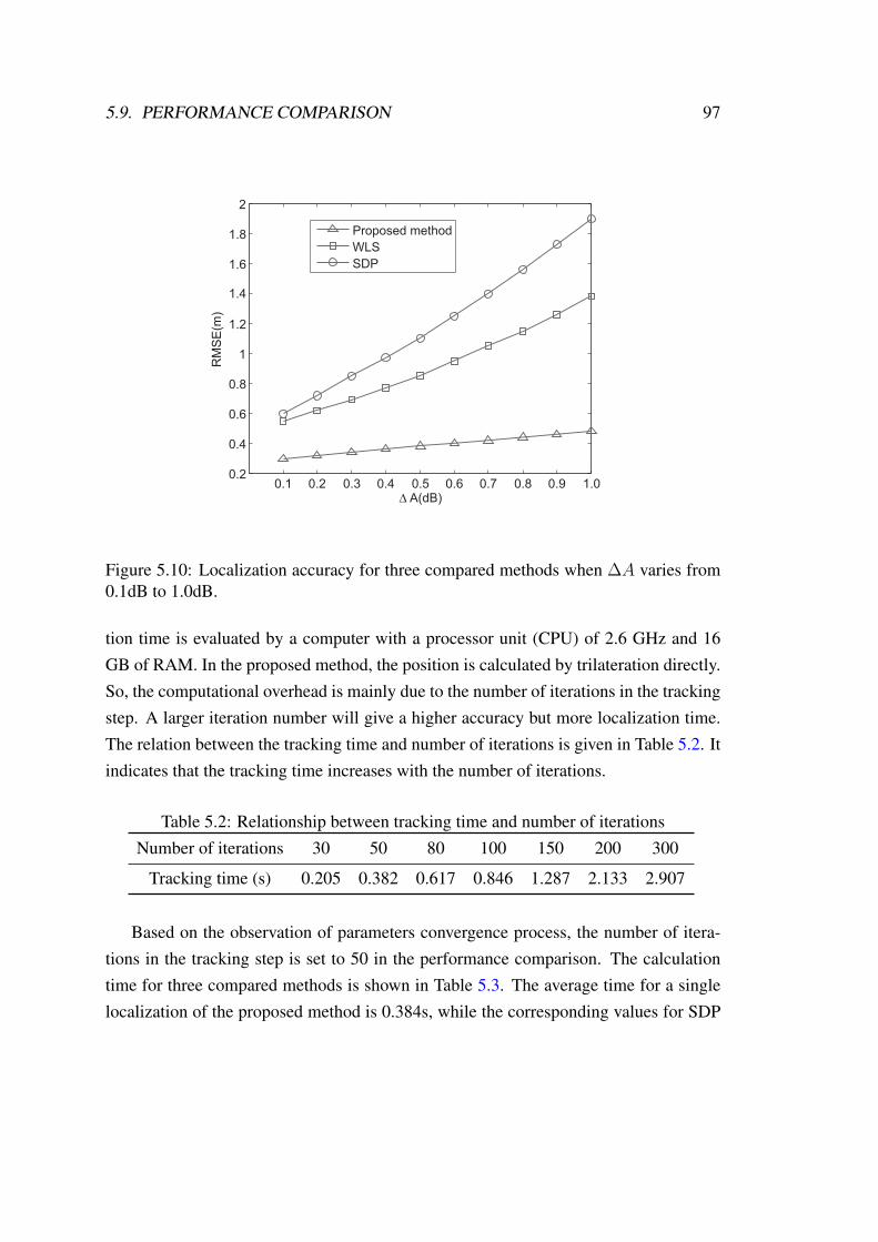
5.9. PERFORMANCE COMPARISON 97
0.1 0.2 0.3 0.4 0.5 0.6 0.7 0.8 0.9 1.00.2
0.4
0.6
0.8
1
1.2
1.4
1.6
1.8
2
Δ A(dB)
RM
SE
(m)
Proposed methodWLSSDP
Figure 5.10: Localization accuracy for three compared methods when ∆A varies from0.1dB to 1.0dB.
tion time is evaluated by a computer with a processor unit (CPU) of 2.6 GHz and 16GB of RAM. In the proposed method, the position is calculated by trilateration directly.So, the computational overhead is mainly due to the number of iterations in the trackingstep. A larger iteration number will give a higher accuracy but more localization time.The relation between the tracking time and number of iterations is given in Table 5.2. Itindicates that the tracking time increases with the number of iterations.
Table 5.2: Relationship between tracking time and number of iterationsNumber of iterations 30 50 80 100 150 200 300
Tracking time (s) 0.205 0.382 0.617 0.846 1.287 2.133 2.907
Based on the observation of parameters convergence process, the number of itera-tions in the tracking step is set to 50 in the performance comparison. The calculationtime for three compared methods is shown in Table 5.3. The average time for a singlelocalization of the proposed method is 0.384s, while the corresponding values for SDP

98 CHAPTER 5. TRACKING STRATEGY
and WLS are 0.032s and 0.024s respectively. We can find that the proposed methodrequires more calculation time than SDP and WLS, due to the tracking step. Moretracking iterations will cause more calculation time. The tradeoff between the local-ization accuracy and the calculation time can be made according to the performancerequirement.
Table 5.3: Calculation time for three compared methodsMethod Proposed method SDP WLS
Average time (s) 0.384 0.032 0.024
5.10 Tracking test
In the tracking test, a large number of measurements have been done in the indoorhall as shown in Figure 3.4. Firstly, the mobile point is placed at (5, 5). Position(5, 5) is considered as a reference point and 300 RSSI samples are acquired in thisposition. Based on these RSSI data, the acquired parameter values are A = −9.39 andη = 2.27. Hereafter, we placed the mobile point at positions (6, 5), (7, 5) and (8, 5) and300 RSSI values are acquired for each position. In the data collecting process, signaltransmission path is changed by modifying the device direction or putting obstacles inthe measurement scenario.
Table 5.4: Localization results and tracked parameters
Real position Estimated position A η
(6, 5) (6.12, 5.26) -9.35 2.26(7, 5) (6.98, 5.13) -9.41 2.28(8, 5) (8.20, 5.08) -9.32 2.25
Based on the acquired RSSI data for each position, the estimated positions andtracked parameters by the proposed method are given in Table 5.4. As shown in Table5.4, for position (6, 5), the estimated position is (6.12, 5.26). This estimated positionmeets the grid correction and tracking condition. By using LMS method, the trackedparameters are A = −9.35 and η = 2.26. Furthermore, similar results are obtained for
5.11. CONCLUSION 99
positions (7, 5) and (8, 5). These results show that the proposed tracking strategy canbe effective. When the mobile point is moving from position (6, 5) to position (8, 5),parameters A and η are changing. In this specific tracking test, the parameters variationis not very large. If the parameters are changing largely, the grid step size should beincreased to guarantee the effectiveness of the proposed tracking strategy, as shown insection 5.5.
5.11 Conclusion
In this chapter, a localization scenario with predefined constrained positions hasbeen described to show the applications of the proposed tracking strategy. To track thevariation of channel parameters, a novel tracking strategy with grid correction based onLMS has been developed to obtain the actual parameters in the monitored indoor re-gion. The experimental RSSI channel model has been used to provide the RSSI valuesand evaluate the tracking strategy. The localization algorithm based on the trilaterationalgorithm and LMS has been presented. The relationship between the localization ac-curacy and sample number of RSSI has been discussed. The simulation results showthe good behavior of the proposed tracking strategy in presence of space-time variationof the propagation channel. To deal with the limitation of the proposed grid correction,the relationship between the grid step size and parameter variation has been analyzed.Compared with the existing SDP and WLS, the proposed tracking strategy exhibits bet-ter localization accuracy but higher computational complexity. Moreover, the trackingtest allows validating the effectiveness of the proposed tracking strategy. In the follow-ing chapter, the thesis will be concluded and future works will be presented.


6Conclusions and perspectives
In this thesis, we focus on RSSI based localization algorithms for indoor applica-tions.
In Chapter 1, the concept and applications of WSNs are described, in addition the re-search direction, the contribution and the organization of the dissertation are described.
In Chapter 2, the state of the art for localization strategies is introduced. The lo-calization approaches in WSNs are classified into two categories: extra modules aidedapproaches and extra modules free approaches. The localization means, such as, GPSmethod cellular network method, infrared device method, ultrasonic wave method, andmicro inertial navigation method are introduced. The methods for measuring the angleor distance, including TOA, TDOA, RSSI and AOA, have been discussed. In addition,the positioning algorithms and optimization methods, such as Triangulation, Multilater-ation, Trilateration, linear least squares (LLS) , non linear least squares (NLS), projec-tion onto convex sets (POCS) and semidefinite programming (SDP) are presented.
Channel model is elaborated in Chapter 3. The experimental channel model is de-duced from RSSI data acquired by real localization system. An experimental local-ization system is built to get real RSSI data. From the observation of RSSI behavior,an experimental RSSI channel model is deduced, which is consistent to the popular
101
102 CHAPTER 6. CONCLUSIONS AND PERSPECTIVES
lognormal shadowing path loss model. Much more data are acquired to observe therelationship between the noise variance and distance. Based on the obtained data, it isindicated that the noise standard deviation increases with the distance. To confirm thistendency, a ray tracing system for an environment similar to the experimental environ-ment is designed to simulate the receiving and transmitting process of RSSI data.
In Chapter 4, three proposed localization algorithms: Three minimum DistancesMethod (TDM), Weighted Three minimum distances Method (WTM) and Weight val-ues Adjustment Method (WAM) based on NLS and multilateration are introduced. Forgetting a good performance, the median value of RSSI is used to obtain the distanceestimate. Multilateration is adopted in the position process. The comparison of TDM,WTM, WAM, LLS, NLS and POCS, in terms of localization accuracy and calculationtime, is presented.
To determine the real predefined position and obtain the actual parameters in themonitored region, a RSSI based parameter tracking strategy for constrained position lo-calization is proposed in Chapter 5. To estimate channel model parameters, Least MeanSquares method (LMS) is associated with the trilateration method. Quantitative criteriaare provided to guarantee the efficiency of the proposed tracking strategy by adjustinggrid resolution according to parameter variation. The simulation results show a goodbehavior of the proposed tracking strategy in presence of space-time variation of thepropagation channel. Compared with the existing SDP and WLS, the proposed track-ing strategy exhibits better localization accuracy but higher computational complexity.Moreover, the tracking test validates the effectiveness of the proposed tracking strategy.
Finally, future work directions are listed as follows:– A real localization scenario, not very different from the experimental setup, will
be constructed to evaluate the proposed tracking strategy and localization algo-rithms.
– In the tracking strategy, the grid can be replaced by other constraint, such as amap.
– Joint techniques will be considered to increase the localization accuracy and re-duce the calculation time. In the future, we will try to joint TOA, DOA and RSSItechniques together, such as exploring joint TOA/RSSI-based algorithm or jointDOA/RSSI-based algorithm, to get a better localization performance.

ARésumé en français des travauxprésentés
A.1 Introduction
Avec l’essor des standards de communications et les progrès d’intégration des sys-tèmes électronique, les réseaux de capteurs sans fils peuvent être couramment déployésdans de nombreuses applications. Lorsque les nœuds du réseau sont mobiles, leur posi-tion doit être estimée car la mesure d’une donnée physique est le plus souvent associéeà la localisation du capteur.
Pour répondre à cette problématique, cette thèse traite d’algorithmes de localisationbasés sur la mesure du RSSI (Received Signal Strength Indicator) dans le contexte desréseaux de capteurs sans fil. L’étude des caractéristiques du RSSI à partir d’un systèmede localisation expérimental permet de construire un modèle nécessaire à la définitionet à l’évaluation des algorithmes. Pour faire face à la faible précision des distances dé-duites du RSSI, nous proposons trois nouveaux algorithmes de localisation basés sur lamultilatération et exploitant des mesures de RSSI moyennées. Ces algorithmes prennenten compte les distances mesurées en fonction de leur fiabilité supposée. Nous dévelop-
103
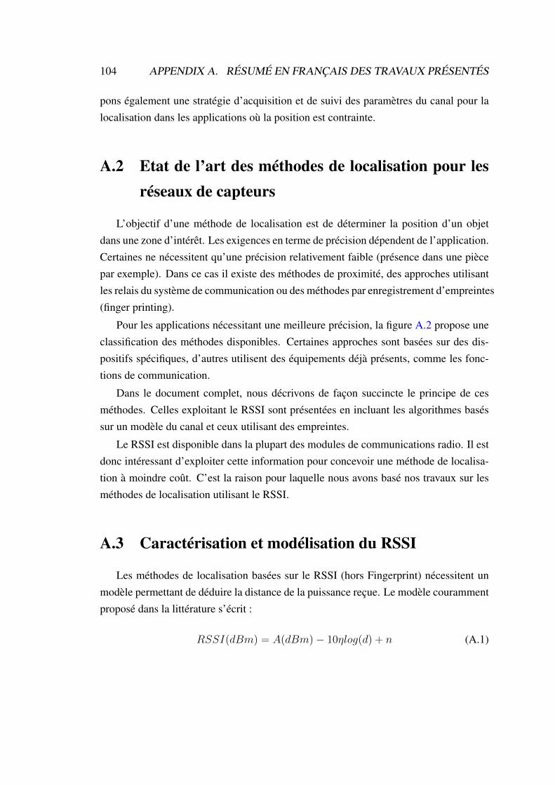
104 APPENDIX A. RÉSUMÉ EN FRANÇAIS DES TRAVAUX PRÉSENTÉS
pons également une stratégie d’acquisition et de suivi des paramètres du canal pour lalocalisation dans les applications où la position est contrainte.
A.2 Etat de l’art des méthodes de localisation pour lesréseaux de capteurs
L’objectif d’une méthode de localisation est de déterminer la position d’un objetdans une zone d’intérêt. Les exigences en terme de précision dépendent de l’application.Certaines ne nécessitent qu’une précision relativement faible (présence dans une piècepar exemple). Dans ce cas il existe des méthodes de proximité, des approches utilisantles relais du système de communication ou des méthodes par enregistrement d’empreintes(finger printing).
Pour les applications nécessitant une meilleure précision, la figure A.2 propose uneclassification des méthodes disponibles. Certaines approches sont basées sur des dis-positifs spécifiques, d’autres utilisent des équipements déjà présents, comme les fonc-tions de communication.
Dans le document complet, nous décrivons de façon succincte le principe de cesméthodes. Celles exploitant le RSSI sont présentées en incluant les algorithmes baséssur un modèle du canal et ceux utilisant des empreintes.
Le RSSI est disponible dans la plupart des modules de communications radio. Il estdonc intéressant d’exploiter cette information pour concevoir une méthode de localisa-tion à moindre coût. C’est la raison pour laquelle nous avons basé nos travaux sur lesméthodes de localisation utilisant le RSSI.
A.3 Caractérisation et modélisation du RSSI
Les méthodes de localisation basées sur le RSSI (hors Fingerprint) nécessitent unmodèle permettant de déduire la distance de la puissance reçue. Le modèle courammentproposé dans la littérature s’écrit :
RSSI(dBm) = A(dBm)− 10ηlog(d) + n (A.1)
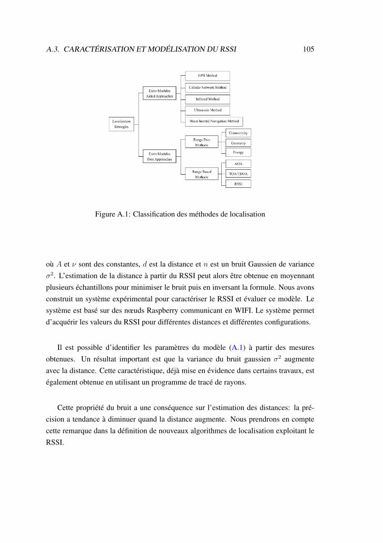
A.3. CARACTÉRISATION ET MODÉLISATION DU RSSI 105
Figure A.1: Classification des méthodes de localisation
où A et ν sont des constantes, d est la distance et n est un bruit Gaussien de varianceσ2. L’estimation de la distance à partir du RSSI peut alors être obtenue en moyennantplusieurs échantillons pour minimiser le bruit puis en inversant la formule. Nous avonsconstruit un système expérimental pour caractériser le RSSI et évaluer ce modèle. Lesystème est basé sur des nœuds Raspberry communicant en WIFI. Le système permetd’acquérir les valeurs du RSSI pour différentes distances et différentes configurations.
Il est possible d’identifier les paramètres du modèle (A.1) à partir des mesuresobtenues. Un résultat important est que la variance du bruit gaussien σ2 augmenteavec la distance. Cette caractéristique, déjà mise en évidence dans certains travaux, estégalement obtenue en utilisant un programme de tracé de rayons.
Cette propriété du bruit a une conséquence sur l’estimation des distances: la pré-cision a tendance à diminuer quand la distance augmente. Nous prendrons en comptecette remarque dans la définition de nouveaux algorithmes de localisation exploitant leRSSI.
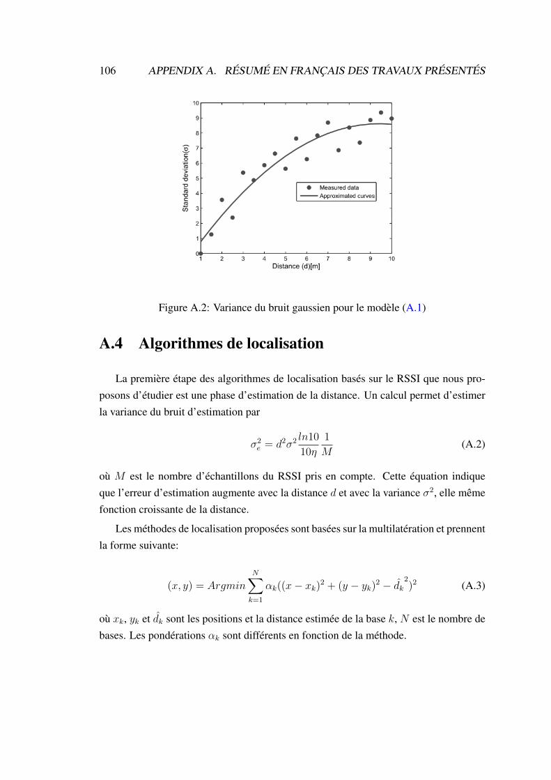
106 APPENDIX A. RÉSUMÉ EN FRANÇAIS DES TRAVAUX PRÉSENTÉS
Figure A.2: Variance du bruit gaussien pour le modèle (A.1)
A.4 Algorithmes de localisation
La première étape des algorithmes de localisation basés sur le RSSI que nous pro-posons d’étudier est une phase d’estimation de la distance. Un calcul permet d’estimerla variance du bruit d’estimation par
σ2e = d2σ2 ln10
10η
1
M(A.2)
où M est le nombre d’échantillons du RSSI pris en compte. Cette équation indiqueque l’erreur d’estimation augmente avec la distance d et avec la variance σ2, elle mêmefonction croissante de la distance.
Les méthodes de localisation proposées sont basées sur la multilatération et prennentla forme suivante:
(x, y) = Argmin
N∑k=1
αk((x− xk)2 + (y − yk)2 − dk2)2 (A.3)
où xk, yk et dk sont les positions et la distance estimée de la base k, N est le nombre debases. Les pondérations αk sont différents en fonction de la méthode.

A.5. STRATÉGIE DE POURSUITE 107
– La méthode TDM, sélectionne les trois plus faibles distances estimées.– La méthode WTM sélectionne les trois plus faibles distances estimées et leur
affecte des pondérations inversement proportionnelles au carré de la distance es-timée et à la variance du bruit estimée.
– La méthode WAM pondère toutes les distances estimées avec des pondérationsidentiques à la méthode WTM.
L’étude comparées des performances de ces méthodes et de méthodes concurrentes dela littérature montre que la méthode WAM fournit les meilleures performances sans quela complexité des calculs ne soit affectée.
A.5 Stratégie de poursuite
Dans les méthodes présentées, la précision du modèle liant le RSSI aux distancesest essentiel. Dans un environnement réel les paramètres de ce modèle vont varier defaçon importante en fonction de l’environnement. Dans cette partie nous proposons,dans un premier temps, d’utiliser une technique d’estimation des paramètres du modèlebasée sur l’algorithme LMS et la présence de nœuds de référence (dont la position estconnue). Nous proposons ensuite de réaliser une poursuite du modèle en supposant quela position du mobile est contrainte par exemple sur une grille.
Le principe est illustré à la figure A.3.– Au départ l’acquisition du modèle est effectuée sur un nœud de référence en util-
isant un algorithme LMS– Après cette phase d’acquisition, les distances sont estimées en utilisant le modèle
de RSSI courant.– L’algorithme de trilatération permet d’estimer la position.– Cette estimation est corrigée en tenant compte de la contrainte de la grille.– L’estimation corrigée est utilisée à l’entrée de l’algorithme LMS pour corriger le
modèle de RSSI.La correction de l’estimation de position n’est possible que si l’erreur d’estimation
initiale est inférieure à la résolution de la grille. Nous avons donc cherché la relationentre la variation des paramètres du modèle et l’erreur de position. On peut en dé-duire la résolution minimale de la grille admissible pour notre algorithme en fonctionde l’environnement.

108 APPENDIX A. RÉSUMÉ EN FRANÇAIS DES TRAVAUX PRÉSENTÉS
Figure A.3: Algorithme de localisation incluant l’estimation du modèle et la poursuite
Figure A.4: Résultats expérimentaux de l’algorithme de localisation incluantl’estimation du modèle et la poursuite
Une comparaison avec d’autres algorithmes n’incluant pas la poursuite du modèlemontre que, lorsque le canal varie, seul notre algorithme permet de maintenir de bonnesperformances. L’algorithme a été testé en utilisant notre système expérimental. Surun espace de 10x10 m2, le point de référence est placé en (5m, 5m). Une premièreacquisition du modèle est effectuée puis le nœud est déplacé. Le canal est modifié enplaçant des obstacles dans la zone de mesure. La résolution de la grille est de 1 m. Letableau de la figure A.4 fournit quelques résultats qui montrent le bon fonctionnementde notre algorithme avec des signaux réels.
A.6 Conclusion
L’objectif du travail présenté était d’étudier des techniques de localisation basées surla mesure du RSSI. Nous avons étudié expérimentalement les propriétés du RSSI et enavons déduit un modèle mettant en évidence le fait que la variance du bruit de mesuredu RSSI augmente avec la distance. Nous avons montré que la variance de l’estimationde la distance était inversement proportionnelle au carré de la distance et à la variance

A.6. CONCLUSION 109
du bruit de mesure. Nous avons proposé des algorithmes basés sur la multilatération etprenant en compte l’imprécision des distances déduites du RSSI. Nous nous sommesintéressés à du modèle de canal et à sa poursuite pour des scénarios d’application où lespositions est contraintes. L’algorithme proposé a été testé sur des données réelles.


List of Tables
3.1 Comparison of sensor node platforms . . . . . . . . . . . . . . . . . . 563.2 Convertion relationship between percentage value and dBm by Cisco . . 593.3 Packet read from interface wlan0 . . . . . . . . . . . . . . . . . . . . . 613.4 Environment information for four cases . . . . . . . . . . . . . . . . . 633.5 Different parameter values for four cases . . . . . . . . . . . . . . . . . 67
4.1 Simulation time for one localization process in milliseconds . . . . . . 81
5.1 Localization accuracy . . . . . . . . . . . . . . . . . . . . . . . . . . 915.2 Relationship between tracking time and number of iterations . . . . . . 975.3 Calculation time for three compared methods . . . . . . . . . . . . . . 985.4 Localization results and tracked parameters . . . . . . . . . . . . . . . 98
111


List of Figures
1.1 Architecture of a typical wireless sensor networks. . . . . . . . . . . . 12
1.2 Application classification for WSNs . . . . . . . . . . . . . . . . . . . 14
2.1 Two steps of localization process . . . . . . . . . . . . . . . . . . . . . 20
2.2 Application classification for WSNs . . . . . . . . . . . . . . . . . . . 21
2.3 Error analysis on DV hop count measurement . . . . . . . . . . . . . . 26
2.4 Principle of APIT algorithm . . . . . . . . . . . . . . . . . . . . . . . 27
2.5 Diagram of tetrahedron algorithm . . . . . . . . . . . . . . . . . . . . 29
2.6 Timing process of the two-way scheme . . . . . . . . . . . . . . . . . . 30
2.7 Terminals deployment of TDOA method . . . . . . . . . . . . . . . . . 32
2.8 Hardware configuration of TDOA . . . . . . . . . . . . . . . . . . . . 33
2.9 Time delay computation model for TDOA . . . . . . . . . . . . . . . . 34
2.10 Angle of arrival measurement. . . . . . . . . . . . . . . . . . . . . . . 37
2.11 Triangulation . . . . . . . . . . . . . . . . . . . . . . . . . . . . . . . 38
2.12 Trilateration . . . . . . . . . . . . . . . . . . . . . . . . . . . . . . . . 40
2.13 Hyperbolic method . . . . . . . . . . . . . . . . . . . . . . . . . . . . 42
2.14 Projection onto Convex Sets . . . . . . . . . . . . . . . . . . . . . . . 46
3.1 Typical sensor node architecture . . . . . . . . . . . . . . . . . . . . . 55
3.2 Raspberry Pi model A . . . . . . . . . . . . . . . . . . . . . . . . . . 56
3.3 Raspberry Pi model B . . . . . . . . . . . . . . . . . . . . . . . . . . 57
3.4 Measurement scenario . . . . . . . . . . . . . . . . . . . . . . . . . . 58
3.5 Diagram of the testing localization system . . . . . . . . . . . . . . . . 58
3.6 Fitting relationship between percentage values and dBm . . . . . . . . 60
3.7 Relationship of the measured RSSI values and distance . . . . . . . . . 62
113

114 LIST OF FIGURES
3.8 Relationship of the noise standard deviation and distance for measureddata . . . . . . . . . . . . . . . . . . . . . . . . . . . . . . . . . . . . 63
3.9 Simulation scenario of ray tracing system . . . . . . . . . . . . . . . . 643.10 Relationship of the simulated RSSI values and distance for case 1 . . . 653.11 Relationship of the simulated RSSI values and distance for case 2 . . . 653.12 Relationship of the simulated RSSI values and distance for case 3 . . . 663.13 Relationship of the simulated RSSI values and distance for case 4 . . . 663.14 Comparison of the linearizion curves for four cases . . . . . . . . . . . 673.15 Relationship of the noise standard deviation and distance based on sim-
ulated data for case 1 . . . . . . . . . . . . . . . . . . . . . . . . . . . 683.16 Relationship between the noise standard deviation and distance based
on simulated data for case 2 . . . . . . . . . . . . . . . . . . . . . . . 693.17 Relationship between the noise standard deviation and distance based
on simulated data for case 3 . . . . . . . . . . . . . . . . . . . . . . . 693.18 Relationship between the noise standard deviation and distance based
on simulated data for case 4 . . . . . . . . . . . . . . . . . . . . . . . 703.19 Comparison between Relationship between the noise standard deviation
and distance based on simulated data for four cases . . . . . . . . . . . 70
4.1 Relationship between σ2e and M for dk = 5. . . . . . . . . . . . . . . . 75
4.2 Relationship between σ2e and M for dk = 8. . . . . . . . . . . . . . . . 76
4.3 Location relationships of three circles in ideal and real conditions . . . 774.4 Grid defining the intersection positions and anchor nodes positions . . 794.5 Localization results for three methods . . . . . . . . . . . . . . . . . . 80
5.1 An application scenario about indoor environment with a set of devicesin it . . . . . . . . . . . . . . . . . . . . . . . . . . . . . . . . . . . . 84
5.2 Grid defining the possible positions . . . . . . . . . . . . . . . . . . . 855.3 Diagram of tracking principle . . . . . . . . . . . . . . . . . . . . . . 905.4 Convergence process of η. . . . . . . . . . . . . . . . . . . . . . . . . 915.5 Convergence process of A . . . . . . . . . . . . . . . . . . . . . . . . 925.6 Relationship of step size and localization error . . . . . . . . . . . . . . 935.7 Relationship between ∆η and s . . . . . . . . . . . . . . . . . . . . . . 945.8 Relationship between ∆A and s . . . . . . . . . . . . . . . . . . . . . 95

LIST OF FIGURES 115
5.9 Localization accuracy for three compared methods when ∆η varies from0.004 to 0.04. . . . . . . . . . . . . . . . . . . . . . . . . . . . . . . . 96
5.10 Localization accuracy for three compared methods when ∆A variesfrom 0.1dB to 1.0dB. . . . . . . . . . . . . . . . . . . . . . . . . . . . 97
A.1 Classification des méthodes de localisation . . . . . . . . . . . . . . . . 105A.2 Variance du bruit gaussien pour le modèle (A.1) . . . . . . . . . . . . . 106A.3 Algorithme de localisation incluant l’estimation du modèle et la poursuite108A.4 Résultats expérimentaux de l’algorithme de localisation incluant l’estimation
du modèle et la poursuite . . . . . . . . . . . . . . . . . . . . . . . . . 108

Publications
Journal1. A RSSI based parameter tracking strategy for constrained position localization,
Jinze Du, Jean-François Diouris and Yide Wang. EURASIP Journal on Advances inSignal Processing. 2017:77. DOI: 10.1186/s13634-017-0512-x
Conference1. An adaptive trilateration localization algorithm based on RSSI model Jinze Du,
Jean-François Diouris and Yide Wang. The third Sino-French Workshop on Informationand Communication Technologies (SIFWICT 2015), Jun 2015, Nantes, France.
2. Novel RSSI-Based Techniques for Indoor Localization, Jinze Du, Jean-FrançoisDiouris and Yide Wang. The IEEE Radio and Antenna Days of the Indian Ocean (RA-DIO), September 2017, Cape town, South Africa.
117


Bibliography
[1] Fredrik Gustafsson and Abdelhak M Zoubir, “Cooperative localization in wsnsusing gaussian mixture modeling: Distributed ecm algorithms,” IEEE Transac-
tions on Signal Processing, vol. 63, no. 6, pp. 1448–1463, 2014.
[2] Jennifer Yick, Biswanath Mukherjee, and Dipak Ghosal, “Wireless sensor net-work survey,” Computer networks, vol. 52, no. 12, pp. 2292–2330, 2008.
[3] Franck L Lewis et al., “Wireless sensor networks,” Smart environments: tech-
nologies, protocols, and applications, pp. 11–46, 2004.
[4] Alan Mainwaring, David Culler, Joseph Polastre, Robert Szewczyk, and JohnAnderson, “Wireless sensor networks for habitat monitoring,” in Proceedings of
the 1st ACM international workshop on Wireless sensor networks and applica-
tions. Acm, 2002, pp. 88–97.
[5] Joseph Polastre, Jason Hill, and David Culler, “Versatile low power media accessfor wireless sensor networks,” in Proceedings of the 2nd international conference
on Embedded networked sensor systems. ACM, 2004, pp. 95–107.
[6] Chris Otto, Aleksandar Milenkovic, Corey Sanders, and Emil Jovanov, “Systemarchitecture of a wireless body area sensor network for ubiquitous health moni-toring,” Journal of mobile multimedia, vol. 1, no. 4, pp. 307–326, 2006.
[7] Hermann Kopetz, “Internet of things,” in Real-time systems, pp. 307–323.Springer, 2011.
[8] Ian F Akyildiz, Weilian Su, Yogesh Sankarasubramaniam, and Erdal Cayirci, “Asurvey on sensor networks,” IEEE Communications magazine, vol. 40, no. 8, pp.102–114, 2002.
119

120 BIBLIOGRAPHY
[9] Ian F Akyildiz, Weilian Su, Yogesh Sankarasubramaniam, and Erdal Cayirci,“Wireless sensor networks: a survey,” Computer networks, vol. 38, no. 4, pp.393–422, 2002.
[10] V Paruchuri, Arjan Durresi, Durga S Dash, and Raj Jain, “Optimal floodingprotocol for routing in ad-hoc networks,” in Proceedings of the IEEE Conference
on Wireless Communications and Networking, 2003.
[11] Satish Verma and Wei Tsang Ooi, “Controlling gossip protocol infection patternusing adaptive fanout,” in Proceedings of 25th IEEE International Conference
on Distributed Computing Systems. IEEE, 2005, pp. 665–674.
[12] Chalermek Intanagonwiwat, Ramesh Govindan, and Deborah Estrin, “Directeddiffusion: a scalable and robust communication paradigm for sensor networks,”in Proceedings of the 6th annual international conference on Mobile computing
and networking. ACM, 2000, pp. 56–67.
[13] Kemal Akkaya and Mohamed Younis, “A survey on routing protocols for wirelesssensor networks,” Ad hoc networks, vol. 3, no. 3, pp. 325–349, 2005.
[14] Brad Karp and Hsiang-Tsung Kung, “Gpsr: Greedy perimeter stateless routingfor wireless networks,” in Proceedings of the 6th annual international conference
on Mobile computing and networking. ACM, 2000, pp. 243–254.
[15] Hu Junping, Jin Yuhui, and Dou Liang, “A time-based cluster-head selectionalgorithm for leach,” in Proceedings of the IEEE Symposium on Computers and
Communications. IEEE, 2008, pp. 1172–1176.
[16] Sachin Sharma, Dharmendra Kumar, and Rajesh Kumar, “Qos-based routingprotocol in wsn,” Advances in Wireless and Mobile Communications, vol. 1, no.1-3, pp. 51–57, 2008.
[17] Jiu-Bin Zhang, Pi-zhuang ZHANG, and Kun-kun DU, “Wireless sensor networkstime synchronization based on gps,” Transducer and Microsystem Technologies,vol. 28, pp. 31–33, 2009.
[18] Azzedine Boukerche, Horacio ABF Oliveira, Eduardo F Nakamura, and Anto-nio AF Loureiro, “Localization systems for wireless sensor networks,” IEEE
wireless Communications, vol. 14, no. 6, 2007.

BIBLIOGRAPHY 121
[19] Anindya S Paul and Eric A Wan, “Rssi-based indoor localization and trackingusing sigma-point kalman smoothers,” IEEE Journal of Selected Topics in Signal
Processing, vol. 3, no. 5, pp. 860–873, 2009.
[20] Mihaela I Chidean, Eduardo Morgado, Eduardo del Arco, Julio Ramiro-Bargueno, and Antonio J Caamaño, “Scalable data-coupled clustering for largescale wsn,” IEEE Transactions on Wireless Communications, vol. 14, no. 9, pp.4681–4694, 2015.
[21] Wendi B Heinzelman, Anantha P Chandrakasan, and Hari Balakrishnan, “Anapplication-specific protocol architecture for wireless microsensor networks,”IEEE Transactions on wireless communications, vol. 1, no. 4, pp. 660–670, 2002.
[22] Theodore S Rappaport et al., Wireless communications: principles and practice,vol. 2, prentice hall PTR New Jersey, 1996.
[23] Loukas Lazos and Radha Poovendran, “Serloc: Secure range-independent local-ization for wireless sensor networks,” in Proceedings of the 3rd ACM workshop
on Wireless security. ACM, 2004, pp. 21–30.
[24] Isaac Amundson and Xenofon Koutsoukos, “A survey on localization for mobilewireless sensor networks,” Mobile entity localization and tracking in GPS-less
environnments, pp. 235–254, 2009.
[25] Nabil M Drawil, Haitham M Amar, and Otman A Basir, “Gps localization accu-racy classification: A context-based approach,” IEEE Transactions on Intelligent
Transportation Systems, vol. 14, no. 1, pp. 262–273, 2013.
[26] Elliott Kaplan and Christopher Hegarty, Understanding GPS: principles and
applications, Artech house, 2005.
[27] Trevor M Ellis, R Barry Bousfield, Lucy A Bissett, Kitman C Dyrting, Geral-dine SM Luk, ST Tsim, Katharine Sturm-Ramirez, Robert G Webster, Yi Guan,and JS Malik Peiris, “Investigation of outbreaks of highly pathogenic h5n1 avianinfluenza in waterfowl and wild birds in hong kong in late 2002,” Avian Pathol-
ogy, vol. 33, no. 5, pp. 492–505, 2004.
[28] Alex Varshavsky, Mike Y Chen, Eyal de Lara, Jon Froehlich, Dirk Haehnel,Jeffrey Hightower, Anthony LaMarca, Fred Potter, Timothy Sohn, Karen Tang,et al., “Are gsm phones the solution for localization?,” in Proceedings of the 7th

122 BIBLIOGRAPHY
IEEE Workshop on Mobile Computing Systems and Applications. IEEE, 2005,pp. 34–42.
[29] Lucia J Zamorano, Lutz Nolte, A Majeed Kadi, and Zhaowei Jiang, “Interac-tive intraoperative localization using an infrared-based system.,” Neurological
research, vol. 15, no. 5, pp. 290–298, 1993.
[30] David J Schlegel, Douglas P Finkbeiner, and Marc Davis, “Maps of dust infraredemission for use in estimation of reddening and cosmic microwave backgroundradiation foregrounds,” The Astrophysical Journal, vol. 500, no. 2, pp. 525, 1998.
[31] Joseph L Rose and Peter B Nagy, “Ultrasonic waves in solid media,” The Journal
of the Acoustical Society of America, vol. 107, no. 4, pp. 1807–1808, 2000.
[32] MG Silk and KF Bainton, “The propagation in metal tubing of ultrasonic wavemodes equivalent to lamb waves,” Ultrasonics, vol. 17, no. 1, pp. 11–19, 1979.
[33] Oliver J Woodman, “An introduction to inertial navigation,” University of Cam-
bridge, Computer Laboratory, Tech. Rep. UCAMCL-TR-696, vol. 14, pp. 15,2007.
[34] John E Bortz, “A new mathematical formulation for strapdown inertial naviga-tion,” IEEE transactions on aerospace and electronic systems, , no. 1, pp. 61–66,1971.
[35] Sassan Alizadeh, Michael W Brandt, and Francis X Diebold, “Range-based es-timation of stochastic volatility models,” The Journal of Finance, vol. 57, no. 3,pp. 1047–1091, 2002.
[36] Mohsen Jamalabdollahi and Seyed Zekavat, “Toa ranging and layer thicknesscomputation in nonhomogeneous media,” IEEE Transactions on Geoscience and
Remote Sensing, vol. 55, no. 2, pp. 742–752, 2017.
[37] Amer Catovic and Zafer Sahinoglu, “The cramer-rao bounds of hybrid toa/rssand tdoa/rss location estimation schemes,” IEEE Communications Letters, vol.8, no. 10, pp. 626–628, 2004.
[38] Slavisa Tomic, Marko Beko, and Rui Dinis, “3-d target localization in wirelesssensor networks using rss and aoa measurements,” IEEE Transactions on Vehic-
ular Technology, vol. 66, no. 4, pp. 3197–3210, 2017.

BIBLIOGRAPHY 123
[39] Dragos Niculescu and Badri Nath, “Ad hoc positioning system (aps) using aoa,”in Proceedings of the Twenty-Second Annual Joint Conference of the IEEE Com-
puter and Communications. Ieee, 2003, vol. 3, pp. 1734–1743.
[40] Jose Velasco, Daniel Pizarro, Javier Macias-Guarasa, and Afsaneh Asaei, “Tdoamatrices: Algebraic properties and their application to robust denoising withmissing data,” IEEE Transactions on Signal Processing, vol. 64, no. 20, pp.5242–5254, 2016.
[41] Li Cong and Weihua Zhuang, “Non-line-of-sight error mitigation in tdoa mobilelocation,” in Proceedings of the IEEE Conference on Global Telecommunica-
tions. IEEE, 2001, vol. 1, pp. 680–684.
[42] Pooyan Abouzar, David G Michelson, and Maziyar Hamdi, “Rssi-based dis-tributed self-localization for wireless sensor networks used in precision agricul-ture,” IEEE Transactions on Wireless Communications, vol. 15, no. 10, pp. 6638–6650, 2016.
[43] Yayoi Sakiyama, Nguyen KN Thao, Nguyen M Giang, Shinji Miyadoh, Duong VHop, and Katsuhiko Ando, “Kineosporia babensis sp. nov., isolated from plantlitter in vietnam,” International journal of systematic and evolutionary microbi-
ology, vol. 59, no. 3, pp. 550–554, 2009.
[44] Daniel Butzke, Robert Hurwitz, Bernd Thiede, Sigrid Goedert, and ThomasRudel, “Cloning and biochemical characterization of apit, a new l-amino acidoxidase from aplysia punctata,” Toxicon, vol. 46, no. 5, pp. 479–489, 2005.
[45] S Chen, AW Palmer, KTV Grattan, and BT Meggitt, “Fringe order identifica-tion in optical fibre white-light interferometry using centroid algorithm method,”Electronics Letters, vol. 28, no. 6, pp. 553–555, 1992.
[46] Dragos Niculescu and Badri Nath, “Ad hoc positioning system (aps),” inProceedings of the IEEE Conference Global Telecommunications. IEEE, 2001,vol. 5, pp. 2926–2931.
[47] Luca Rigazio, Brice Tsakam, and J-C Junqua, “An optimal bhattacharyya cen-troid algorithm for gaussian clustering with applications in automatic speechrecognition,” in Proceedings of the IEEE International Conference on Acous-
tics, Speech, and Signal Processing. IEEE, 2000, vol. 3, pp. 1599–1602.

124 BIBLIOGRAPHY
[48] Tian He, Chengdu Huang, Brian M Blum, John A Stankovic, and Tarek F Ab-delzaher, “Range-free localization and its impact on large scale sensor networks,”ACM Transactions on Embedded Computing Systems (TECS), vol. 4, no. 4, pp.877–906, 2005.
[49] Hongbin Tan and Feng Liu, “Research and implementation of apit positioningalgorithm in wsn,” in Proceedings of the 9th IEEE International Conference on
Fuzzy Systems and Knowledge Discovery (FSKD), 2012, pp. 2212–2215.
[50] Nirupama Bulusu, John Heidemann, and Deborah Estrin, “Gps-less low-costoutdoor localization for very small devices,” IEEE personal communications,vol. 7, no. 5, pp. 28–34, 2000.
[51] Hongyang Chen, Pei Huang, Marcelo Martins, Hing Cheung So, and KaoruSezaki, “Novel centroid localization algorithm for three-dimensional wirelesssensor networks,” in Proceedings of the 4th International Conference on Wire-
less Communications, Networking and Mobile Computing. IEEE, 2008, pp. 1–4.
[52] Jan Blumenthal, Ralf Grossmann, Frank Golatowski, and Dirk Timmermann,“Weighted centroid localization in zigbee-based sensor networks,” in Proceed-
ings of the IEEE International Symposium on Intelligent Signal Processing.IEEE, 2007, pp. 1–6.
[53] Paolo Pivato, Luigi Palopoli, and Dario Petri, “Accuracy of rss-based centroidlocalization algorithms in an indoor environment,” IEEE Transactions on Instru-
mentation and Measurement, vol. 60, no. 10, pp. 3451–3460, 2011.
[54] Bo Zhu and Shu Chen, “An improved centroid localization algorithm for wirelesssensor network,” Chinese Journal of Sensors and Actuators, vol. 6, pp. 024, 2010.
[55] Guangjie Han, Huihui Xu, Trung Q Duong, Jinfang Jiang, and Takahiro Hara,“Localization algorithms of wireless sensor networks: a survey,” Telecommuni-
cation Systems, pp. 1–18, 2013.
[56] James J Caffery, “A new approach to the geometry of toa location,” in Proceed-
ings of the 52nd IEEE Conference on Vehicular Technology, 2000, vol. 4, pp.1943–1949.
[57] Ismail Guvenc and Chia-Chin Chong, “A survey on toa based wireless localiza-tion and nlos mitigation techniques,” IEEE Communications Surveys & Tutorials,vol. 11, no. 3, 2009.
BIBLIOGRAPHY 125
[58] Saipradeep Venkatraman, James Caffery, and Heung-Ryeol You, “A novel toa lo-cation algorithm using los range estimation for nlos environments,” IEEE Trans-
actions on Vehicular Technology, vol. 53, no. 5, pp. 1515–1524, 2004.
[59] Jan-Jaap Van de Beek, Magnus Sandell, and Per Ola Borjesson, “Ml estimationof time and frequency offset in ofdm systems,” IEEE transactions on signal
processing, vol. 45, no. 7, pp. 1800–1805, 1997.
[60] Paul C Chestnut, “Emitter location accuracy using tdoa and differential doppler,”IEEE Transactions on Aerospace and Electronic Systems, , no. 2, pp. 214–218,1982.
[61] Ryota Yamasaki, Atsushi Ogino, Tsuyoshi Tamaki, Takaki Uta, Naoto Mat-suzawa, and Takeshi Kato, “Tdoa location system for ieee 802.11 b wlan,” inProceedings of the IEEE Conference on Wireless Communications and Network-
ing, 2005, vol. 4, pp. 2338–2343.
[62] KC Ho, “Bias reduction for an explicit solution of source localization using tdoa,”IEEE Transactions on Signal Processing, vol. 60, no. 5, pp. 2101–2114, 2012.
[63] Kutluyil Dogancay and DA Gray, “Bias compensation for least-squares multi-pulse tdoa localization algorithms,” in Proceedings of the IEEE International
Conference on Intelligent Sensors, Sensor Networks and Information Processing,2005, pp. 51–56.
[64] Wing-Kin Ma, Ba-Ngu Vo, Sumeetpal S Singh, and Adrian Baddeley, “Trackingan unknown time-varying number of speakers using tdoa measurements: A ran-dom finite set approach,” IEEE Transactions on Signal Processing, vol. 54, no.9, pp. 3291–3304, 2006.
[65] Cesare Alippi and Giovanni Vanini, “A rssi-based and calibrated centralized lo-calization technique for wireless sensor networks,” in Proceedings of Fourth
Annual IEEE International Conference on Pervasive Computing and Communi-
cations Workshops. IEEE, 2006, pp. 5–pp.
[66] Ossi Kaltiokallio, Maurizio Bocca, and Lasse M Eriksson, “Distributed rssi pro-cessing for intrusion detection in indoor environments,” in Proceedings of the
9th ACM/IEEE International Conference on Information Processing in Sensor
Networks. ACM, 2010, pp. 404–405.

126 BIBLIOGRAPHY
[67] Ahmed Faheem, Reino Virrankoski, and Mohammed Elmusrati, “Improving rssibased distance estimation for 802.15. 4 wireless sensor networks,” in Proceedings
of the IEEE International Conference on Wireless Information Technology and
Systems (ICWITS). IEEE, 2010, pp. 1–4.
[68] Mohit Saxena, Puneet Gupta, and Bijendra Nath Jain, “Experimental analysisof rssi-based location estimation in wireless sensor networks,” in Proceedings
of the 3rd International Conference on Communication Systems Software and
Middleware and Workshops. IEEE, 2008, pp. 503–510.
[69] David C Jenn, “Transmission equation for multiple cooperative transmitters andcollective beamforming,” IEEE Antennas and Wireless Propagation Letters, vol.7, pp. 606–608, 2008.
[70] Chun-Pang Wu and Hen-Wai Tsao, “A 110-mhz 84-db cmos programmable gainamplifier with integrated rssi function,” IEEE Journal of Solid-State Circuits,vol. 40, no. 6, pp. 1249–1258, 2005.
[71] Hyo-Sung Ahn and Wonpil Yu, “Environmental-adaptive rssi-based indoor lo-calization,” IEEE Transactions on Automation Science and Engineering, vol. 6,no. 4, pp. 626–633, 2009.
[72] Yapeng Wang, Xu Yang, Yutian Zhao, Yue Liu, and Laurie Cuthbert, “Blue-tooth positioning using rssi and triangulation methods,” in Proceedings of the
IEEE Conference on Consumer Communications and Networking. IEEE, 2013,pp. 837–842.
[73] LC San Martin De Viale, AoA Viale, S Nacht, and M_ Grinstein, “Experimen-tal porphyria induced in rats by hexachloro-benzene. a study of the porphyrinsexcreted by urine,” Clinica Chimica Acta, vol. 28, no. 1, pp. 13–23, 1970.
[74] Abdalla OA Ahmed, Moawia M Mukhtar, Marly Kools-Sijmons, Ahmed H Fa-hal, Sybren de Hoog, Bert Gerrits van den Ende, Eduard E Zijlstra, Henri Ver-brugh, AM El Sir, Ahmed M Elhassan, et al., “Development of a species-specificpcr-restriction fragment length polymorphism analysis procedure for identifica-tion ofmadurella mycetomatis,” Journal of clinical microbiology, vol. 37, no. 10,pp. 3175–3178, 1999.
[75] Maurice S Bartlett, “Periodogram analysis and continuous spectra,” Biometrika,vol. 37, pp. 1–16, 1950.
BIBLIOGRAPHY 127
[76] Jack Capon, “High-resolution frequency-wavenumber spectrum analysis,” Pro-
ceedings of the IEEE, vol. 57, no. 8, pp. 1408–1418, 1969.
[77] Kenneth Levenberg, “A method for the solution of certain non-linear problemsin least squares,” Quarterly of applied mathematics, vol. 2, no. 2, pp. 164–168,1944.
[78] Eduardo Cassano, Francesco Florio, Floriano De Rango, and Salvatore Marano,“A performance comparison between roc-rssi and trilateration localization tech-niques for wpan sensor networks in a real outdoor testbed.,” in Proceedings of
the IEEE on Symposium Wireless Telecommunications, 2009, pp. 1–8.
[79] Yiu-Tong Chan and KC Ho, “A simple and efficient estimator for hyperboliclocation,” IEEE Transactions on signal processing, vol. 42, no. 8, pp. 1905–1915, 1994.
[80] Claes Johnson and Juhani Pitkäranta, “An analysis of the discontinuous galerkinmethod for a scalar hyperbolic equation,” Mathematics of computation, vol. 46,no. 173, pp. 1–26, 1986.
[81] Ismail Guvenc, Sinan Gezici, Fujio Watanabe, and Hiroshi Inamura, “Enhance-ments to linear least squares localization through reference selection and ml es-timation,” in Proceedings of the IEEE Conference on Wireless Communications
and Networking. IEEE, 2008, pp. 284–289.
[82] Nemai C Karmakar et al., “Chipless rfid tag localization,” IEEE Transactions on
Microwave Theory and Techniques, vol. 61, no. 11, pp. 4008–4017, 2013.
[83] Yue Wang, “Linear least squares localization in sensor networks,” Eurasip jour-
nal on wireless communications and networking, vol. 2015, no. 1, pp. 51, 2015.
[84] Hing Cheung So, “Source localization: Algorithms and analysis,” Handbook of
Position Location: Theory, Practice, and Advances, pp. 25–66, 2011.
[85] Sinan Gezici, Ismail Guvenc, and Zafer Sahinoglu, “On the performance of lin-ear least-squares estimation in wireless positioning systems,” in Proceedings of
the IEEE International Conference on Communications. IEEE, 2008, pp. 4203–4208.
[86] Patrizia Fanara, Mary R Hodel, Anita H Corbett, and Alec E Hodel, “Quantitativeanalysis of nuclear localization signal (nls)-importin α interaction through fluo-

128 BIBLIOGRAPHY
rescence depolarization evidence for auto-inhibitory regulation of nls binding,”Journal of Biological Chemistry, vol. 275, no. 28, pp. 21218–21223, 2000.
[87] Philip E Gill and Elizabeth Wong, “Sequential quadratic programming methods,”in Mixed integer nonlinear programming, pp. 147–224. Springer, 2012.
[88] Alfred O Hero and Doron Blatt, “Sensor network source localization via projec-tion onto convex sets (pocs),” in Proceedings of IEEE International Conference
on Acoustics, Speech, and Signal Processing. IEEE, 2005, vol. 3, pp. iii–689.
[89] Doron Blatt and Alfred O Hero, “Energy-based sensor network source localiza-tion via projection onto convex sets,” IEEE Transactions on Signal Processing,vol. 54, no. 9, pp. 3614–3619, 2006.
[90] Pratik Biswas and Yinyu Ye, “Semidefinite programming for ad hoc wirelesssensor network localization,” in Proceedings of the 3rd international symposium
on Information processing in sensor networks. ACM, 2004, pp. 46–54.
[91] Pratik Biswas, Tzu-Chen Lian, Ta-Chung Wang, and Yinyu Ye, “Semidefiniteprogramming based algorithms for sensor network localization,” ACM Transac-
tions on Sensor Networks (TOSN), vol. 2, no. 2, pp. 188–220, 2006.
[92] Rong-Hou Wu, Yang-Han Lee, Hsien-Wei Tseng, Yih-Guang Jan, and Ming-Hsueh Chuang, “Study of characteristics of rssi signal,” in Proceedings of the
IEEE International Conference on Industrial Technology. IEEE, 2008, pp. 1–3.
[93] Xinrong Li, “Rss-based location estimation with unknown pathloss model,”IEEE Transactions on Wireless Communications, vol. 5, no. 12, 2006.
[94] A Bahillo, S Mazuelas, J Prieto, P Fernandez, RM Lorenzo, and EJ Abril, “Hy-brid rss-rtt localization scheme for wireless networks,” in Proceedings of the
International Conference on Indoor Positioning and Indoor Navigation. IEEE,2010, pp. 1–7.
[95] Santiago Mazuelas, Alfonso Bahillo, Ruben M Lorenzo, Patricia Fernandez,Francisco A Lago, Eduardo Garcia, Juan Blas, and Evaristo J Abril, “Robust in-door positioning provided by real-time rssi values in unmodified wlan networks,”IEEE Journal of selected topics in signal processing, vol. 3, no. 5, pp. 821–831,2009.
BIBLIOGRAPHY 129
[96] Bodhibrata Mukhopadhyay, Sanat Sarangi, and Subrat Kar, “Performance evalu-ation of localization techniques in wireless sensor networks using rssi and lqi,” inProceedings of the Twenty First National Conference on Communications (NCC).IEEE, 2015, pp. 1–6.
[97] Fazli Subhan, Salman Ahmed, and Khalid Ashraf, “Extended gradient predictorand filter for smoothing rssi,” in Proceedings of 16th IEEE International Confer-
ence on Advanced Communication Technology (ICACT), 2014, pp. 1198–1202.
[98] Yong Tian, Zhenan Tang, and Yan Yu, “Third-order channel propagation model-based indoor adaptive localization algorithm for wireless sensor networks,” IEEE
Antennas and Wireless Propagation Letters, vol. 12, pp. 1578–1581, 2013.
[99] Forough Yaghoubi, Ali-Azam Abbasfar, and Behrouz Maham, “Energy-efficientrssi-based localization for wireless sensor networks,” IEEE Communications Let-
ters, vol. 18, no. 6, pp. 973–976, 2014.
[100] Reza Monir Vaghefi, Mohammad Reza Gholami, R Michael Buehrer, and Erik GStrom, “Cooperative received signal strength-based sensor localization with un-known transmit powers,” IEEE Transactions on Signal Processing, vol. 61, no.6, pp. 1389–1403, 2013.
[101] Begumhan Turgut and Richard P Martin, “Localization for indoor wireless net-works using minimum intersection areas of iso-rss lines,” in Proceedings of the
32nd IEEE Conference on Local Computer Networks. IEEE, 2007, pp. 962–972.
[102] Jie Yin, Qiang Yang, and Lionel Ni, “Adaptive temporal radio maps for indoorlocation estimation,” in Proceedings of the Third IEEE International Conference
on Pervasive Computing and Communications. IEEE, 2005, pp. 85–94.
[103] Luís Felipe M de Moraes and Bruno Astuto A Nunes, “Calibration-free wlanlocation system based on dynamic mapping of signal strength,” in Proceedings
of the 4th ACM international workshop on Mobility management and wireless
access. ACM, 2006, pp. 92–99.
[104] Julie Yixuan Zhu, Anny Xijia Zheng, Jialing Xu, and Victor OK Li, “Spatio-temporal (st) similarity model for constructing wifi-based rssi fingerprinting mapfor indoor localization,” in Proceedings of the International Conference on In-
door Positioning and Indoor Navigation (IPIN). IEEE, 2014, pp. 678–684.

130 BIBLIOGRAPHY
[105] Bodhibrata Mukhopadhyay, Sanat Sarangi, and Subrat Kar, “Novel rssi evalua-tion models for accurate indoor localization with sensor networks,” in Proceed-
ings of the Twentieth National Conference on Communications (NCC). IEEE,2014, pp. 1–6.
[106] Seon Yeong Han, Nael B Abu-Ghazaleh, and Dongman Lee, “Efficient and con-sistent path loss model for mobile network simulation,” Biological Cybernetics,vol. 24, no. 3, pp. 1774–1786, 2016.
[107] Vladimir Vujovic and Mirjana Maksimovic, “Raspberry pi as a wireless sensornode: performances and constraints,” in Proceedings of the 37th International
Convention on Information and Communication Technology, Electronics and Mi-
croelectronics (MIPRO). IEEE, 2014, pp. 1013–1018.
[108] Sheikh Ferdoush and Xinrong Li, “Wireless sensor network system design usingraspberry pi and arduino for environmental monitoring applications,” Procedia
Computer Science, vol. 34, pp. 103–110, 2014.
[109] Fung Po Tso, David R White, Simon Jouet, Jeremy Singer, and Dimitrios PPezaros, “The glasgow raspberry pi cloud: A scale model for cloud computinginfrastructures,” in Proceedings of the 33rd International Conference on Dis-
tributed Computing Systems Workshops (ICDCSW). IEEE, 2013, pp. 108–112.
[110] Jiuqiang Xu, Wei Liu, Fenggao Lang, Yuanyuan Zhang, and Chenglong Wang,“Distance measurement model based on rssi in wsn,” Wireless Sensor Network,vol. 2, no. 08, pp. 606, 2010.
[111] Jungang Zheng, Chengdong Wu, Hao Chu, and Peng Ji, “Localization algorithmbased on rssi and distance geometry constrain for wireless sensor network,” inProceedings of the International Conference on Electrical and Control Engineer-
ing (ICECE). IEEE, 2010, pp. 2836–2839.
[112] Mohammad Reza Gholami, Erik G Ström, Henk Wymeersch, and Mats Ryd-ström, “On geometric upper bounds for positioning algorithms in wireless sensornetworks,” Signal Processing, vol. 111, pp. 179–193, 2015.
[113] Quentin H Spencer, Brian D Jeffs, Michael A Jensen, and A Lee Swindlehurst,“Modeling the statistical time and angle of arrival characteristics of an indoormultipath channel,” IEEE Journal on Selected areas in communications, vol. 18,no. 3, pp. 347–360, 2000.
BIBLIOGRAPHY 131
[114] Safa Hamdoun, Abderrezak Rachedi, and Abderrahim Benslimane, “Compara-tive analysis of rssi-based indoor localization when using multiple antennas inwireless sensor networks,” in Proceedings of the International Conference on
Selected Topics in Mobile and Wireless Networking (MoWNeT). IEEE, 2013, pp.146–151.
[115] Paula Tarrío, Ana M Bernardos, and José R Casar, “Weighted least squares tech-niques for improved received signal strength based localization,” Sensors, vol.11, no. 9, pp. 8569–8592, 2011.
[116] Vijendra Mishra and Gaurav Chaitanya, “Analysis of lms, rls and smi algorithmon the basis of physical parameters for smart antenna,” in Proceedings of the
IEEE Conference on IT in Business, Industry and Government (CSIBIG). IEEE,2014, pp. 1–4.
[117] Yue Wang and KC Ho, “An asymptotically efficient estimator in closed-formfor 3-d aoa localization using a sensor network,” IEEE Transactions on Wireless
Communications, vol. 14, no. 12, pp. 6524–6535, 2015.
[118] Cort J Willmott and Kenji Matsuura, “Advantages of the mean absolute error(mae) over the root mean square error (rmse) in assessing average model perfor-mance,” Climate research, vol. 30, no. 1, pp. 79–82, 2005.
[119] Robin Wentao Ouyang, Albert Kai-Sun Wong, and Chin-Tau Lea, “Receivedsignal strength-based wireless localization via semidefinite programming: Non-cooperative and cooperative schemes,” IEEE Transactions on Vehicular Technol-
ogy, vol. 59, no. 3, pp. 1307–1318, 2010.
[120] Gang Wang, H Chen, Youming Li, and Ming Jin, “On received-signal-strengthbased localization with unknown transmit power and path loss exponent,” IEEE
Wireless Communications Letters, vol. 1, no. 5, pp. 536–539, 2012.


Thèse de Doctorat
Jinze DUIntérieur Techniques de localisation pour les réseaux de capteurs sans fil
Indoor localization techniques for wireless sensor networks
RésuméCette thèse traite d’algorithmes de localisation baséssur la mesure du RSSI (Received Signal StrengthIndicator) pour des applications intérieures dans desréseaux de capteurs sans fil. L’étude descaractéristiques du RSSI à partir d’un système delocalisation expérimental, permet de construire unmodèle de canal RSSI de type atténuation lognormale.Pour faire face à la faible précision des distancesdéduites de RSSI, nous proposons trois nouveauxalgorithmes de localisation à l’intérieur des bâtimentsbasés sur la multilatération et les mesures de RSSImoyennées. Ces algorithmes pondèrent les distancesmesurées en fonction de leur fiabilité supposée. Nousdéveloppons également, une stratégie d’acquisition etde suivi des paramètres du canal pour la localisationdans des applications où la position est contrainte.Pour estimer les paramètres du modèle de canal, laméthode des moindres carrés moyens (LMS) estassociée à une méthode de trilatération. Des critèresquantitatifs sont fournis pour garantir l’efficacité de lastratégie de suivi en proposant un compromis entre larésolution de la contrainte et la variation desparamètres du modèle. Les résultats de simulationmontrent un bon comportement de la stratégie depoursuite proposée en présence d’une variationspatio-temporelle du canal de propagation. Parrapport aux algorithmes existants, une meilleureprécision de localisation est obtenue au prix d’un peuplus de temps de calcul. La stratégie proposée estégalement testée expérimentalement.
AbstractIn this thesis, the author focused on RSSI basedlocalization algorithms for indoor applications inwireless sensor networks. Firstly, from the observationof RSSI behavior based on an experimentallocalization system, an experimental RSSI channelmodel is deduced, which is consistent to the popularlognormal shadowing path loss model. Secondly, thisthesis proposes three indoor localization algorithmsbased on multilateration and averaged RSSI. In thesealgorithms, the measured distances are weightedaccording to their assumed accuracy. Lastly, a RSSIbased parameter tracking strategy for constrainedposition localization is proposed. To estimate channelmodel parameters, least mean squares method (LMS)is associated with the trilateration method.Quantitative criteria are provided to guarantee theefficiency of the proposed tracking strategy byproviding a tradeoff between the constraint resolutionand parameter variation. The simulation results showa good behavior of the proposed tracking strategy inpresence of space-time variation of the propagationchannel. Compared with the existing RSSI basedalgorithms, the proposed tracking strategy exhibitsbetter localization accuracy but consumes morecalculation time. In addition, experimental tracking testis performed to validate the effectiveness of theproposed tracking strategy.
Mots clésLocalisation, RSSI, Réseau de capteurs dans fils,Trilatération, Poursuite.
Key WordsLocalization, RSSI, WSNs, Trilateration, Tracking.
UNIVERSITÉ BRETAGNE LOIRE