Improving the time resolution of surfzone bathymetryusing in situ altimeters

Melissa Moulton & Steve Elgar & Britt Raubenheimer

Received: 14 September 2013 /Accepted: 25 March 2014# Springer-Verlag Berlin Heidelberg 2014

Abstract Surfzone bathymetry often is resolved poorly intime because watercraft surveys cannot be performed whenwaves are large, and remote sensing techniques have limitedvertical accuracy. However, accurate high-frequency bathy-metric information at fixed locations can be obtained fromaltimeters that sample nearly continuously, even duringstorms. A method is developed to generate temporally andspatially dense maps of evolving surfzone bathymetry byupdating infrequent spatially dense watercraft surveys withthe bathymetric changemeasured by a spatially sparse array ofnearly continuously sampling altimeters. The update methodis applied to observations of the evolution of shore-perpendicular rip current channels (dredged in Duck, NC,2012) and shore-parallel sandbars (observed in Duck, NC,1994). The updated maps are compared with maps made bytemporally interpolating the watercraft surveys, and withmaps made by spatially interpolating the altimeter measure-ments at any given time. Updated maps of the surfzone ripchannels and sandbars are more accurate than maps obtainedby using either only watercraft surveys or only the altimetermeasurements. Hourly altimeter-updated bathymetric esti-mates of five rip channels show rapid migration and infillevents not resolved by watercraft surveys alone. For a 2-month observational record of sandbars, altimeter-updatedmaps every 6 h between nearly daily surveys improve thetime resolution of rapid bar-migration events.

Keywords Altimeters . Bathymetric surveys . Rip channels .

Rip currents . Sandbars . Surf zone

1 Introduction

Surfzone bathymetry controls wave shoaling, refraction, andbreaking, and consequently affects wave-driven setup, near-shore currents, and the transport of nutrients, biota, and sed-iment. On energetic sandy coastlines, the seafloor can evolvedramatically within several hours. Cusps and channels asso-ciated with rip currents (Chen et al. 1999; Haller et al. 2002;MacMahan et al. 2006; Austin et al. 2010; Dalrymple et al.2011; and many others) migrate and flatten quickly in thepresence of wave-driven alongshore flows (Falqués et al.2000; van Enckevort and Ruessink 2003; Garnier et al.2013), and sandbars migrate rapidly offshore during storms(Thornton et al. 1996; Gallagher et al. 1998a; Hsu et al. 2006;and many others). Nearshore hydrodynamic model results aresensitive to bathymetry (Plant et al. 2002, 2009), and often thelargest model errors are associated with poor temporal resolu-tion of bathymetric changes (Wilson et al. 2010). Obtainingsurfzone bathymetry with sufficient spatial and temporal sam-pling for developing, testing, and improving models, especial-ly during energetic conditions, is challenging.

Watercraft with surveying equipment are used to map thesurfzone seafloor with high spatial resolution (Birkemeier andMason 1984; MacMahan 2001; Dugan et al. 2001; Lippmannand Smith 2008), but these techniques usually are restricted tocalm conditions preceding and following storms, and thus thetemporal evolution of the largest bathymetric changes is notresolved well. During times when waves and bubbles preventwatercraft surveys, observations of evolving bathymetry maybe obtained by remote sensing techniques (Holman and Haller2013). By taking advantage of the depth-dependence of wavespeed and dissipation (van Dongeren et al. 2008; Holman et al.2013) and by assimilating in situ observations (Wilson et al.2010; Birrien et al. 2013), video observations may be used toestimate bathymetry at low cost and with reasonable verticalaccuracy (roughly 0.5 m, Holman and Haller 2013), which has

Responsible Editor: Bruno Castelle

This article is part of the Topical Collection on the 7th InternationalConference on Coastal Dynamics in Arcachon, France 24-28 June 2013

M. Moulton (*) : S. Elgar :B. RaubenheimerWoods Hole Oceanographic Institution, Woods Hole, MA, USAe-mail: melissarmoulton@gmail.com

Ocean DynamicsDOI 10.1007/s10236-014-0715-8

allowed for long-term monitoring of changes in the position ofnearshore sand bars and rip current channels (Lippmann andHolman 1989; Holman et al. 1993; Holland et al. 1997;Ruessink et al. 2000; van Enckevort et al. 2004; Holmanet al. 2006; Gallop et al. 2011; and many others). However,remotely sensed bathymetric inversion techniques usually arelimited to timescales of several days or longer and to spatialscales of 10 m or greater (van Dongeren et al. 2008; Holmanet al. 2013), and for some studies video observationsmay not beavailable or may not provide sufficient vertical accuracy.

In contrast, in situ altimeters provide accurate, nearly con-tinuous estimates of the distance between the sensor and theseafloor (Gallagher et al. 1996, 1998a, b). Usually, altimetersare deployed at a limited number of locations, and thus maynot resolve the spatial structure of the seafloor evolution,while watercraft surveys offer good spatial resolution, but ata limited number of times. Combining the two data sets shouldproduce higher temporal resolution maps of the seafloor thanobtained with infrequent spatially dense watercraft surveys,and higher spatial resolutionmaps than obtained with spatiallysparse altimeters. Data with irregular sampling and errors maybe combined with interpolation and mapping techniques(Ooyama 1987; Plant et al. 2002) and data assimilationmethods (van Dongeren et al. 2008; Holman et al. 2013;Wilson et al. 2010; Birrien et al. 2013). Here, a method ispresented that seeks an accurate estimate of a spatiallysmoothed bathymetry by updating spatially dense watercraftsurveys with temporally continuous, spatially sparse altimeterestimates of seafloor elevation change. The method is tested fortwo datasets that span a wide range of variability in the surfzone, including observations of migrating and filling shore-perpendicular rip channels dredged on a sandy ocean beachnear Duck, NC in 2012, and observations of a migrating shore-parallel sandbar near Duck, NC in 1994. The methods used formeasuring (Section 2) and mapping (Section 3) surfzone ba-thymetry are described, and are tested and applied for the ripchannel (Section 4) and sandbar (Section 5) datasets, and theresults are discussed and summarized (Section 6).

2 Direct estimation of seafloor location

2.1 Vehicle surveys

Small personal watercraft can navigate effectively in shallowwater under moderate waves, and when equipped with GPSand bottom-finding sonar can be used to map surfzone ba-thymetry (MacMahan 2001; Dugan et al. 2001; Lippmann andSmith 2008). A jetski (waverunner) was used in the 2012Duck, NC experiment discussed in Section 4. Typically, wa-tercraft surveys are performed along cross- and alongshoretracks, with spacing between tracks and sample density alongtracks dependent on the experimental design and survey

system. The horizontal accuracy of differential GPS systemsis about 0.25 to 0.50 m. The vertical accuracy from individualbed-level estimates from acoustic pings is about 0.05 to0.10 m (this includes 0.02–0.04 m errors in GPS verticalestimates, and 0.03–0.06 m errors in the estimate of thedistance from the transducer to the bed, but does not includethe effects of short-horizontal-scale features such as wave-orbital ripples and megaripples). Watercraft provide estimatesof the seafloor location over a wide area in a relatively shorttime, but often are less effective in the surf zone because theapproximately 10 km/h speed precludes averaging (at any onelocation) of many acoustic returns, some of which can beobscured by breaking-wave induced bubbles.

In contrast with acoustic systems that are degraded bybubbles, amphibious vehicles can be used to map the seaflooreven in an active surf zone. For the 1994 Duck, NC experi-ment described in Section 5, the CRAB, a tall three-wheeledvehicle that is tracked with a laser survey system (Birkemeierand Mason 1984) was used to map the seafloor. The CRABoperates from above the high-tide line to 8-m water depth inwaves up to 2 m high, travels at up to 4 km/h, has verticalaccuracy of 0.03 to 0.10 m, and has a horizontal resolution ofroughly 8 m (the spacing between the wheels) (Birkemeierand Mason 1984).

2.2 Fixed altimeters

Fixed acoustic devices (altimeters) also may be used to findthe seafloor (Gallagher et al. 1996). Altimeters can be de-ployed during calm conditions, and continue to sample duringlarge wave events when watercraft cannot operate. Moreover,by sampling relatively rapidly at one location, the acousticreturns from a fixed altimeter can be used to find the seaflooreven if bubbles obscure the signal most of the time or if thetransducer is coming in and out of the water in wave troughs atlow tide. Altimeters have been used to investigate sandbarevolution (Gallagher et al. 1998a; Elgar et al. 2001; Hoefeland Elgar 2003; Henderson et al. 2004; Hsu et al. 2006; andmany others), bottom roughness (Feddersen et al. 2003;Gallagher et al. 2005), and bedforms (Gallagher et al.1998b). Although fixed altimeters can find the seafloor inthe surf zone, it is difficult to deploy and maintain more thana few dozen instruments (resulting in limited spatial resolu-tion) for more than a few months. Altimeter estimates of theseafloor location can be biased owing to survey errors in thevertical elevation of the acoustic transducers (0.04–0.10m). Inaddition, there are randomly distributed errors owing to thefinite bin size of the acoustic returns and to the algorithm usedto detect the bottom in a time series of noisy acoustic returns.

In the 2012 Duck, NC experiment, single-beam acousticaltimeters recently developed at the Woods Hole Oceano-graphic Institution (WHOI altimeter, 1 MHz beam, 2 Hz echoamplitude averaged to 1 min, 0.01 m vertical bins) were used

Ocean Dynamics

to monitor changes in the surfzone seafloor. During a perfor-mance test, a WHOI altimeter deployed on a pipe in the surfzone found the distance from the transducer to the bed (Fig. 1)with roughly 0.05 m accuracy even in the presence of bubblesin a saturated surf zone (offshore significant wave height of2.5 m, surfzone wave height of 1.5 m). Older versions of thealtimeters (used in the 1994 Duck, NC experiment) performedwell during large storms with offshore wave heights greaterthan 4.0 m (Gallagher et al. 1996, 1998a).

The backscatter strength from acoustic Doppler currentprofilers (ADCP) also may be used to find the seafloor. Forexample, a Nortek Aquadopp (three 2 MHz beams, 1-min-average echo amplitude in 0.10m bins averaged over the threebeams) sampling in a saturated surf zone (during the 2012,Duck NC experiment) usually found the bottom within onebin (Moulton et al. 2013), although the bottom signal wasweaker and less robust to bubbles than the signal from thefaster-sampling WHOI Altimeter.

3 Bathymetric mapping methods

3.1 Spatially dense watercraft surveys

The time to complete a watercraft survey is short relative to thetimescale of morphological evolution, and thus the bed-levelestimates are treated as a snapshot of the bathymetry at time tS,where tS is the time of the middle of the survey. At each surveytime tS, there is a spatially dense and irregularly sampled set ofbed-level observations. The observations can be interpolated toform an estimate of the bathymetry ZS(x,y,tS) at a set of regu-larly spaced spatial coordinates (x,y). If multiple surveys areavailable, the time evolution of the bathymetry could be esti-mated by interpolating in both space and time to form atestimate of the bathymetry ZS(x,y,t) at a set of times t. Properties(e.g., smoothness, agreement with observations) of the mappedbathymetry ZS may be controlled by the choice of interpolationweights in space and time (see Appendix).

For the watercraft survey data presented here, spatial inter-polation weights are chosen with a scale-controlled objectivemapping method (Ooyama 1987; Plant et al. 1999) to accountfor unresolved features such as ripples and megaripples. Theinterpolation weights are found assuming a Gaussian covari-ance function with scales Lx (in the cross-shore) and Ly (in thealongshore), a spatially and temporally uniform variance VS

(the average variance estimated from all observations), and anobservation error εO. The observation error εO includes themeasurement error in the bed level estimated by each acousticreturn, plus the root-mean-square (rms) amplitude of featureswith length scales less than Lx and Ly (see Appendix). Fordense sampling (many observations within a radius Lx or Ly),computation timemay be reduced by binning the observationsprior to mapping, where the error for each binned value isestimated assuming each bottom return is an independentbathymetric estimate. A mean beach slope (computed fromall observations) is removed from the observations beforemapping, and added back after mapping, such that the esti-mate approaches the mean profile far from observations (seeAppendix). The resulting maps are a smooth estimate of thebathymetry resolving scales greater than or equal to Lx and Ly.A map of the estimated errors εS(x,y,tS) is computed for eachwatercraft survey map (see Appendix). The bathymetry at anarbitrary time ZS(x,y,t) can be estimated by linearly interpo-lating (inverse separation weighting, see Appendix) betweentwo surveys.

3.2 Temporally dense altimeter bed levels

Altimeters sample nearly continuously, providing temporallydense estimates of the seafloor location. At each altimeterlocation (xA,yA), where xA and yA are the cross- and alongshorecoordinates of the altimeter, there is an estimate of the bedlevel at a set of times. Interpolation is used to compute anestimate of the bathymetry ZA(x,y,t) on a regular grid (x,y) at aset of times t, and properties of the bathymetric estimate arecontrolled by the choice of the interpolation weights, whichare found with a scale-controlled objective mapping method.To reduce computation time, the spatiotemporal interpolationis separated into two steps by assuming space-time separabil-ity of the covariance (effectively ignoring small and poorlyconstrained space-time interactions in the covariance betweenthe widely separated altimeters) (Genton 2007). First, thealtimeter bed levels are interpolated in time to yield ZT(xA,yA,t). The interpolation is performed assuming a Gaussiantemporal covariance with timescale T, a spatially and tempo-rally uniform variance VT (the average variance estimatedfrom all observations, equal to VS), and measurement rmserror εrms (the error in the estimate of the distance from thetransducer to the bed plus the rms amplitude of unresolvedscales). A linear trend is removed from the time series prior tointerpolating, and added back after interpolating. If the

a b

Fig. 1 Amplitude of acoustic returns from the WHOI altimeter (colorscale on right) as a function of depth below the altimeter (Δz) and timefor (a) 7 days (black curve is seafloor location) and (b) 3 min of data. The* on the time axis of (a) (between time=4 and time=5 days) correspondsto the time of the time series in (b)

Ocean Dynamics

timescale T is chosen to be larger than the time between bed-level estimates and larger than the period of migratingbedforms, the temporal interpolation step leads to smoothedtime series with rms error εT(xA,yA,t)<εrms owing to averagingover random measurement errors and migrating ripples. Abias error εbias (associated with measurements of the verticalelevation of the transducer) is added to the error estimate forthe interpolated time series. Next, at each time, the time-interpolated bed-level estimates are interpolated in space as-suming a Gaussian spatial covariance with scales Lx and Ly, aspatially and temporally uniform variance VA (equal to VS),and a measurement error εT(xA,yA,t)+εbias. A mean beachslope (computed from all observations) is removed from theobservations before interpolation, and added back after inter-polation, such that the estimate approaches the mean profilefar from observations (see Appendix). Ideally, altimeter arraysare designed such that sensors are spaced more densely thanone half of the decorrelation scale of the features of interest,but logistical difficulties often lead to undersampling, and thusthere are regions far from altimeters where insufficient bathy-metric information is available (and interpolation weightsapproach zero). The spatial interpolation yields a set of mapsZA(x,y,t) and an error estimate εA(x,y,t).

3.3 Update method for combining all observations

At the times of surveys, it is expected that the spatiallyinterpolated watercraft surveys are the best estimate of thebathymetry, because the maps made from the spatially densesurvey data have smaller errors than the interpolated altimeterdata. In between the survey times, the temporally interpolatedsurveys are a good estimate of bathymetry that changes rough-ly constantly in time. However, nearshore bathymetric evolu-tion can be highly variable in time, including rapid and largechanges during storms when watercraft surveying is not pos-sible. The altimeter maps resolve variable (and rapid) rates ofchange, but have larger vertical errors than the survey maps,which have no bias and average bed-level estimates over asmall area. Alternatively, watercraft survey and altimeter bed-level estimates can be combined to create a single set of mapswith known accuracy. One approach is to use space-timeobjective mapping (Bretherton et al. 1976; Ooyama 1987;Rybicki and Press 1992; Plant et al. 1999, 2002) of all thebed-level estimates. Here, an alternative approach is presentedthat “updates” infrequent watercraft surveys with altimeterdata. The spatial pattern of seafloor change is estimated usingaltimeter data, and added to the mapped watercraft surveys toyield an updated bathymetric estimate at another time. Unlikespace-time objective mapping, the maps made using the up-date method are equal to the spatially mapped surveys at thesurvey times, and by using the bed-level change estimated byaltimeters, rather than the bed level itself, bias errors in thealtimeter bed-level estimates are removed.

To implement the update method, first the bed-level changeCA at each time t before or after each survey time tS isestimated from the time-mapped altimeter time series:

CA xA; yA; tS ; tð Þ ¼ ZA xA; yA; tð Þ − ZA xA; yA; tSð Þ ð1Þ

The error in the change signal εCA(xA,yA, t) is as-sumed to be equal to the error in the mapped timeseries, εCA(xA,yA, t)=εT(xA,yA, t). Next, at each time, thechange estimates are mapped in space assuming aGaussian covariance with length scales Lx and Ly, a spatiallyuniform variance VC [estimated from the change CA(xA,yA,tS,t) between tS and t], and an observation error εCA. No mean ortrend is removed from CA(xA,yA,tS,t) prior to mapping, so thatthe change signal estimate approaches zero far from observa-tions. This process yields a gridded estimate of the changeC(x,y,tS,t) since each survey with estimated errors εC(x,y,tS,t).

Each mapped spatially dense survey is “updated” to othertimes by adding the mapped change:

ZU x; y; tS ; tð Þ ¼ ZS x; y; tSð Þ þ C x; y; tS ; tð Þ ð2Þ

The error of the updated map is estimated as a sum of theerrors of the survey and the change signal:

εU x; y; tS ; tð Þ ¼ εS x; y; tSð Þ þ εC x; y; tS ; tð Þ ð3Þ

The method described in Eq. 2 “updates” a spatially densesurvey either forward or backward in time to form an estimateof the bathymetry at another time. This method is referred toas the forward-backward update method.

When multiple dense surveys are available, a weighted-update method may be used. The bathymetry at each timeZUW(x,y,t) is computed as a weighted sum of the maps up-dated from each survey:

ZUW x; y; tð Þ ¼XtS

W ZS x; y; tSð Þ þ C x; y; tS ; tð Þ½ � ð4Þ

whereW are the weights. The errors are estimated as a weight-ed sum of the errors of the updated maps:

εUW x; y; tð Þ ¼XtS

W εS x; y; tSð Þ þ εC x; y; tS ; tð Þ½ � ð5Þ

The weights chosen here are proportional to the time sep-aration between the time of interest t and the survey times tS,with the weights for the surveys immediately preceding andfollowing the time t summing to one, and all other surveysweighted zero. For this choice of inverse distance weighting,the bathymetric estimate at survey times is equal to ZS(x,y,tS).Between survey times, the bed-level estimate approaches themapped altimeter bed-level estimate at time t plus a weighted

Ocean Dynamics

offset between the mapped altimeter bed-level estimates andthe surveys at the nearest survey times [note that C(x,y,tS,t)≈ZA(x,y,t)−ZA(x,y,tS)]. The bathymetric estimate far (severaltimes Lx or Ly) from altimeters approaches a weighted sumof the surveys (note that the mapped C(x,y,tS,t) approacheszero far from the altimeters).

3.4 Method assessment

In addition to comparing the estimated interpolation errors, themethods are tested by comparing the mapped estimates withan independent estimate of the true bathymetry. A mappedsurvey at a particular survey time is set aside as independent“ground truth” for the methods attempting to reconstruct thebathymetry at that time. Comparisons are made only in theregion for which the surveys have errors below a specifiedthreshold (in regions with poor survey coverage, the mappedsurvey may not be an accurate representation of the truebathymetry). At each time, the differences (at the set of spatialmapping coordinates) between the true bathymetry and amapped bathymetric estimate are referred to as the “recon-struction residuals,” and the rms residuals are referred to as the“reconstruction errors” εR. The average reconstruction errorover all comparisons is denoted �εR. For the forward-backwardupdatemethod (Eq. 2), only one watercraft survey is usedwiththe altimeters to estimate the bathymetry, and all other surveysare used as ground truth. For the weighted-update method(Eq. 4), as well as for temporally interpolating between twodense surveys, the ground truth survey is one that was

obtained between two other surveys that are used to recon-struct the bathymetry at any time between them. Thus, anycombination of three surveys can be used to test the weighted-update and the temporal interpolation methods. The first andlast surveys are used to estimate the bathymetry at the time ofthe middle survey, which is the ground truth.

4 Rip channel bathymetric estimates

4.1 Overview of field observations and mapping of dredgedrip channels

The propellers from a Vietnam-era landing craft were used todredge large shore-perpendicular channels in 1- to 3-m waterdepth on a long straight Atlantic Ocean beach at the US ArmyCorps of Engineers Field Research Facility near Duck, NC,USA. Five channels were dredged in July and August 2012(Fig. 2 shows two of the five channels). Pressure sensorscolocated with current meters (both sampled at 2 Hz) andcurrent profilers (1-min averages) were deployed near thebed in and outside of the channels (Fig. 2), and bathymetricevolution was recorded by a watercraft survey system andaltimeters. The channels were on average 2-m deep, 30-mwide in the alongshore, and 50-m long in the cross-shore.The ambient bathymetry was either a terrace (e.g., Fig. 2c, d,e, f) or a small sandbar (0.5–1 m trough to crest) (e.g.,Fig. 2a,b on the south side of the channel), and the averagetidal range was 1 m. Bedforms observed by divers and

b c

100 150 200 620

670

720d

Alo

ngsh

ore

coor

dina

te (

m)

100 150 200

e

Cross−shore coordinate (m)

100 150 200

f

Map

ping

err

or (

m)

0

0.05

0.1

0.15

0.2

0.25

0.3

620

670

720aN

Fig. 2 Contours of mapped water depth (relative to mean sea level, blackcurves every 0.5 m in depth, the thick curves are −1.5 m) and estimatedinterpolation errors (colors, scale on right) from watercraft surveys forchannels dredged on 18 July (top row: a, b, c) and 24 July 2012 (bottomrow: d, e, f) as a function of cross- and alongshore coordinate, with theshoreline on the left side of each panel and north toward the top. Thesurvey times for the first dredged channel are a 18 July 18:00 EDT(shortly after dredging), b 20 July 10:00, and c 23 July 12:00. The survey

times for the second dredged channel are d 24 July 12:00 (shortly afterdredging), e 26 July 14:00, and f 27 July 15:00.Crosses show positions ofaltimeters, which were colocated with a pressure gauge and a currentmeter or current profiler. Three other dredged channels (not shown) hadarrays similar to the channel dredged on 24 July (d, e, f). For all surveymaps, the errors usually are 0.01–0.05 cm, except near the shorelinewhere the density of survey tracks (not shown) was reduced and errorsare as great at 0.3 m

Ocean Dynamics

documented in detail for previous studies at this site includedsmall wave ripples and larger-scale megaripples with heightsof order 0.1–0.5 m (rms amplitude ~0.1 m), horizontal lengthscales of order 1–10 m, and propagation speeds of 0.3–1.2 m/h (Gallagher et al. 1998b, 2005). Significant waveheights [4 times the standard deviation (std dev) of sea-surface-elevation fluctuations in the frequency (f) band 0.05<f<0.30 Hz] just offshore of the channels ranged from 0.5 to1.5 m and wave directions (Kuik et al. 1988) ranged fromapproximately −35° to +35° relative to shore normal. Both ripcurrent circulation patterns (0.1 to 1.0 m/s hour-averagedjet speeds) and alongshore flows over the channels (0.1 to1.0 m/s hour-averaged speeds) were observed, and the ba-thymetry tended to evolve rapidly in response to the largerwaves and stronger flows (Moulton et al. 2013).

Surveys were performed daily with a personal watercraft(waverunner) except when waves were too large for safeoperations. The 24 personal watercraft surveys for the fivechannel experiments (three surveys each for the two channelsshown in Fig. 2, and six surveys each for the other threechannels) spanned roughly 200 m in the alongshore (centeredat the channels), and extended from the mean shoreline (sur-veys usually were performed at high tide) to about 100 to200 m offshore (Moulton et al. 2013). The 1- to 3-h-longsurveys were conducted along cross- and alongshore orientedtracks, each separated by approximately 5 m with a sampleevery 0.1 m along each track.

To study the coupled evolution of the channels and flows,the survey data were mapped (Fig. 2) to a 2-m spatial grid (x,y) spanning 100 m in the alongshore (centered at the channels)and 100 m in the cross-shore (approximately from the meanshoreline to 3-m water depth). The surveys were mapped as adeviation from an average linear beach slope for each channellocation (average slopes found from a fit to all observationsfor each channel location ranged from 0.019 to 0.025). Tospeed the computations, raw survey data were averaged over2×2 m bins prior to mapping. The error in each bin is esti-mated as the sample error divided by the square root of thenumber of observations in the bin. The binned data weremapped using scale-controlled objective mapping with Lx=Ly= 9 m, VS= 0.08 m2, and an observation error (prior tobinning) of εO= 0.20 m. The decorrelation scales are foundfrom Gaussian fits to the autocovariance of cross- and along-shore bathymetric profiles, and on average were 5 m in thecross-shore (std dev=2 m) and 6 m in the alongshore (stddev=2 m). Across the deepest channel cross-sections, thealongshore decorrelation scale is on average 9 m (std dev=2 m). Here, Lx=Ly= 9m are used in the mapping to resolve therip channels and smooth over smaller features (megaripplewavelengths may be 1–10 m). The variance VS is the averagevariance of the deviations of smooth bathymetric estimatesfrom the mean beach slope (estimated using all observations).The observation error εO was chosen to account for vertical

errors in the bed location (0.10 m) and for the amplitude ofunresolved features (0.10 m rms bedform amplitude). Theresult is 24 bathymetric estimates (at the survey times) ZS(x,y,tS) (Fig. 2, contours) and a corresponding set of error esti-mates εS(x,y,tS) (Fig. 2, colors). The errors for the surveys aresmall (~0.02 m) except near the shoreline where survey tracksare sparse or absent. An estimate of the bathymetry betweensurvey times on a 1-h time (t) grid [ZS(x,y,t)] spanning theobservational record was found using the temporal-inverse-distance weighting described in Section 3.1. The error in ZS(x,y,t) is expected to be equal to εS(x,y,tS) at the survey times andincrease quadratically with increasing time separation fromsurveys, and thus to become larger than the signal variancewhen more than one decorrelation time scale away from anysurvey (e.g., Mastroianni and Milovanović 2008), but noformal error estimate is made here.

Estimates of the seafloor elevation were obtained everyminute from an array of altimeters (as few as 6 and as manyas 14 sensors) with roughly 5 to 30 m spacing centered at thechannel (arrays for two channels are shown in Fig. 2, the threechannels not shown had 10–14 altimeters in an array similar tothat shown in Fig. 2d, e, f). The arrays were designed toresolve the flows and bathymetry in the rip channels [expectedto have scales of O(10 m) in the cross- and alongshore direc-tions] and on the adjacent cross-shore terrace and bar structure[expected to have scales of O(10 m) in the cross-shore andscales of O(50 m) or longer in the alongshore far from thechannels]. Sensors were spaced most densely across the chan-nels, where the flows and bathymetry were expected to varymost rapidly in space and time. Two types of acoustic altim-eters were deployed. At most locations, the bed level wasestimated with the single-beam acoustic altimeters recentlydeveloped at WHOI, and at a few locations the bed elevationwas estimated using a downward-looking Nortek Aquadoppprofiler mounted above the seafloor. The altimeter time seriesare mapped in time to the 1-h grid t with a scale-controlledobjective mapping method with T= 6 h, VT= 0.08 m2 (theaverage variance estimated from all observations), and mea-surement rms error εrms= 0.10 m (assumed the same for bothtypes of altimeters). The timescale Twas chosen to resolve thefastest migration events, and is large enough to average overseveral periods of most migrating bedforms [although somebedformsmay take as long as 36 h to pass under each altimeter(Gallagher et al. 2005)]. The temporal mapping step led tosmoothed time series with rms error εT~ 0.013 m <εrms. Thiserror may be an underestimate if there are large megaripples(the analysis assumes that the observation errors are correlatedon scales smaller than T, which is not the case for long, slow-moving bedforms). A bias error (error in the mean, owing toGPS and hand-measurement errors) εbias= 0.10 m is added tothe error estimate for each mapped altimeter time series. Thetime-mapped bed-level estimates are mapped in space (usingthe same grid as the mapped surveys) as a deviation from a

Ocean Dynamics

linear beach slope (same as the slope removed in the mappedsurveys) assuming a Gaussian spatial covariance with scalesLx=Ly= 9m,VA= 0.08m2, and measurement error [εT+εbias]~0.11 m. The resulting maps ZA(x,y,t) have estimated errorsεA(x,y,t) ranging from ~0.1 m near the altimeter locations to~0.3 m far from the altimeters.

The survey and altimeter data are combined using theweighted-update method described in Section 3.3, yieldinggridded (2 m, 1 h) estimates of the bathymetry ZUW(x,y,t) andthe associated error εUW(x,y,t). The weighted-update mapshave errors that are equal to the survey errors at survey timesεUW(x,y, tS)=εS(x,y, tS), and are smallest near the altimeterlocations at all other times. The size of the errors in theupdated maps increases with time since a watercraft survey,and is scaled by the variance of the change since the nearestsurveys. To test the update method, all possible forward-backward update maps ZU(x,y,tS,t) [and the correspondingerror estimate εU(x,y,tS,t)] (Eq. 2, using each survey) and alltestable weighted-update maps (Eq. 4, using the first and thirdsurvey for all possible sets of three surveys) are computed. Forcomparison with the weighted-update maps, all testable time-interpolated surveys are computed.

4.2 Assessment of rip channel maps

The accuracy of maps made with watercraft surveys alone(Section 3.2), altimeters alone (Section 3.3), and surveysupdated with altimeter-estimated change (Section 3.4) isassessed for the 24 watercraft surveys (three surveys for eachof two channels, and six surveys each for the other threechannels) of evolving rip channels. First, the forward-backward updated maps are assessed and compared with thealtimeter maps. Next, the weighted-update maps are assessedand compared with the forward-backward updated maps, thealtimeter maps, and time-interpolation of surveys. The errorsare computed in the region for which survey errors are smallerthan 0.05 m (regions near the shoreline with large surveyerrors are excluded).

There are 51 pairs (and thus 102 test cases by goingforward or backward in time) of temporally separated water-craft surveys, where one survey in the pair is used with Eq. 2to estimate the bathymetry at the time of the other survey,which is used as ground truth to test the estimate. In addition,bathymetry estimated from altimeter bed levels at the time ofthe ground truth survey was compared with the ground truth.The forward-backward updated maps have smaller averagereconstruction errors (εR,U= 0.14 m) than the altimeter maps(εR,A= 0.18 m). The average rms difference between the pairsof spatially dense surveys is 0.15 m.

There are 62 sets of three temporally separated wa-tercraft surveys, where the first and third survey areused to estimate the bathymetry at the time of thesecond survey (the ground truth), using inverse-time

weighting of the watercraft surveys or by updating withaltimeter information either forward in time from thefirst survey (“forward updated map”), backward in timefrom the third survey (“backward updated map”), or aweighted combination (Eq. 4). In addition, at the timeof the second survey, an altimeter-based estimate of thebathymetry was compared with the second survey. Theweighted-update maps have average reconstruction er-rors (� �������������εR,UW = 0.08 m) that are smaller than errors inthe forward and backward updated maps ( ����������εR ,U=0 . 1 2 m ) , t h e a l t im e t e r - i n t e r p o l a t i o n m a p s(��������εR,A= 0.16 m), and temporal interpolation between sur-veys (��������εR,S= 0.09 m). The average rms difference be-tween final and initial spatially dense surveys is 0.19 m.

As an example, the bathymetry surveyed on 26 July(Fig. 3a) is estimated from a survey 2 days earlier (24 July12:00, Fig. 2d) and a survey 1 day later (27 July 15:00, Fig. 2f)using the weighted-update (Eq. 4) (Fig. 3b) and altimeter-interpolation (Fig. 3c) methods. The weighted-update maphas smaller errors (Fig. 3b, colors) than the altimeter-interpolation map (Fig. 3c, colors). The rms change betweenthe 24 and 27 July surveys was 0.29 m (Fig. 3d). The averageresiduals (difference from the ground truth survey) for theupdated map (Fig. 3e) [0.11 m, similar to the average estimat-ed errors (0.14 m) for the updated map] are smaller than theaverage residuals for the altimeter map (Fig. 3f) [0.21 m,similar to the average estimated errors (0.26 m) for the altim-eter map]. The spatial pattern of the residuals (Fig. 3e, f,colors) is not consistent with the error estimate (Fig. 3b, c, colors), likely because the bathymetry varies morerapidly in time (Fig. 3d) and space (Fig. 3a, comparerelatively uniform shoals with the channel) near thechannels and the shoreline than elsewhere, in contrastwith the assumption of a uniform signal variance. Themapping methods and error estimates may be improvedby estimating a non-uniform spatial variance (larger atthe channel position). However, the channels migrate,and thus a non-uniform spatial variance that is accurateat one time may be a poor estimate at another time.

To study the evolution of the channels with highertemporal resolution, channel cross-sections (depth versusalongshore coordinate) are extracted from the two-dimensional maps (at the cross-shore coordinate nearestthe densest cross-channel altimeter spacing) for each ofthe mapping methods, resulting in an estimate of thechannel cross-section every hour for each channel andeach method. The cross-sectional profiles may have dif-ferent error statistics than the two-dimensional maps,because the sensor-spacing is denser on average, andthe bathymetry may vary more rapidly in space and timefor the cross-section of a deep section of the channelthan for the full two-dimensional domain. Similar to thetwo-dimensional maps, the accuracy of the one-

Ocean Dynamics

dimensional cross-section estimates was compared fortime-interpolation of surveys, mapping of altimeter data,and the forward-backward and weighted-update methods.

For the 51 pairs of temporally separated watercraft surveys(102 comparisons), the forward-backward updated maps haveslightly smaller average reconstruction errors (����������εR,U = 0.17 m)than the altimeter maps (��������εR,A = 0.18 m). The average rmsdifference between final and initial spatially dense surveys is0.20 m. For the 62 sets of three temporally separated water-craft surveys, the weighted-update maps have average recon-struction errors (� �������������εR,UW = 0.10 m) that are smaller than theforward and backward updated maps (��������εR,U = 0.15), the altim-eter maps (��������εR,A = 0.15 m), and the weighted surveys ��������εR,S =

0.11 m). The average rms difference between pairs of spatiallydense surveys is 0.24 m.

The three methods (weighted-update, altimeter-interpolation, and time-interpolation of dense surveys) areused to reconstruct the bathymetry on 30 June (Fig. 4). Thesurvey on 30 June (Fig. 4, solid black curve) has small errors(Fig. 4, gray shading around black curve), and thus is a goodrepresentation of the true bathymetry. The surveys completed28 June (Fig. 4, dashed black curve) and 5 July (Fig. 4, dottedblack curve) are used with altimeter change estimates in theweighted-update method (Eq. 4) to produce estimates of thebathymetry (Fig. 4, blue curve) and associated errors (Fig. 4,blue shading). Altimeter interpolation also is used to estimate

740760780800820840

−2.6

−2.4

−2.2

−2

−1.8

−1.6

−1.4

−1.2

Dep

th (

m, r

elat

ive

to m

ean

sea

leve

l)

Alongshore coordinate (m)

Altimeter positions Survey: 28 June 13:00 Survey: 05 July 12:00 Survey: 30 June 07:00 Altimeters: 30 June 07:00 Updated: 30 June 07:00 Survey Interp: 30 June 07:00

Fig. 4 Depth of seafloor acrossthe channel versus alongshorecoordinate from watercraftsurveys on 28 June 13:00 (blackdashed curve), 30 June 07:00(ground truth, solid black curve),and 5 July 12:00 (dotted blackcurve), and estimated for 30 June07:00 using the weighted-update(blue curve), altimeter-interpolation (red curve), andtime-interpolation of the 28 Juneand 05 July surveys (green curve).Shaded areas are 1 std dev errorsfor the estimated bathymetries.Crosses show alongshorepositions of altimeters

b c

100 150 200 620

670

720d

Alo

ngsh

ore

coor

dina

te (

m)

100 150 200

e

Cross−shore coordinate (m)

100 150 200

f

Map

ping

err

or (

m)

0

0.05

0.1

0.15

0.2

0.25

0.3

620

670

720aN

Fig. 3 Contours of mapped water depth (relative to mean sea level, blackcurves every 0.5 m in depth, the thick contours are −1.5 m) and errors(colors, scale on right) on 26 July 14:00 for a a mapped watercraft survey,b a weighted-update map (surveys at 24 July 12:00 and 27 July 15:00 areused to form the estimate, see Fig. 2d, f), and c an altimeter map. d Themapped watercraft survey on 26 July 14:00 (black contours) and the

magnitude of change between the surveys on 24 July 12:00 and 27 July15:00, and (e and f) contours of water depth (black contours) andmagnitude of residuals with the survey on 26 July 14:00 using (e) aweighted-update map and (f) an altimeter map. All maps are a function ofcross- and alongshore coordinate, with the shoreline on the left side ofeach panel. Crosses show positions of altimeters

Ocean Dynamics

the bathymetry on 30 June (Fig. 4, red curve) and associatederrors (Fig. 4, red shading). Interpolating between the sur-veys on 28 June and 5 July (Fig. 4, green curve) is similarto the weighted-update method (Fig. 4, blue curve). Therms reconstruction error (rms difference with the surveyon 30 June) for the weighted-update map is 0.07 m (sim-ilar to the average estimated error 0.08 m), for the altim-eter maps is 0.15 m (similar to the average estimated error0.22 m), and for the time-interpolation of surveys is0.07 m. The rms difference between the surveys on 28June and 05 July is 0.21 m.

4.3 Application of update method to rip channel cross-sectionevolution

The cross-sections of the hourly updated maps can be used toinvestigate the temporal evolution of the channels between thespatially dense surveys. For the channel dredged on 18 July,dense surveys show that the channel filled and moved north-ward (toward larger alongshore coordinate) between 20 and23 July (Fig. 2, compare panels b and c). However, thesesurveys do not resolve the higher-frequency temporal changescaused by the relatively large waves and rip current that wereobserved during the several days between dense surveys. Inthe absence of additional information, it must be assumed thebathymetry evolved uniformly between the times of the densesurveys. In contrast, the cross-sections estimated by updatingdense surveys with changes observed by the altimeters (Fig. 5,gray curves are every 3 h) indicate that the rates of channelinfill and migration (Fig. 6) varied non-uniformly in time.

Gaussian fits to hourly updated cross-sections are used as aproxy to determine the channel position (Fig. 6a, usuallywithin one grid cell of the location of the minimum of theprofile) and channel depth (Fig. 6b), and (not shown) channelwidth and ambient bed elevation. Confidence intervals (grayshading in Fig. 6) are found from the distribution of parame-ters from a series of fits to 300 curves generated by summingthe updated maps with random errors drawn from aGaussian distribution with std dev given by the estimat-ed mapping rms error.

Flows in the rip channel fluctuated with the tidal elevation,with the highest flows occurring near low tide when wavebreaking was strongest on the shallow sides. When the chan-nel center moved north of the mid-way point between thecenter and the northern sensor (Fig. 6a, 21–23 July), themaximum measured offshore-directed flow (not shown) alsomoved north, from near the center of the channel (y=662 m)on 21 July to the northern edge of the channel (y=674 m)(Moulton et al. 2013). The channel filled by almost 1 m duringthe 27 h that the channel center migrated north (from 21 July12:00 until 22 July 15:00, Figs. 5 and 6). Significant waveheights just offshore of the channel were between 0.5 and1.0 m, and wave directions were within 15° of shore normalbetween 21 July 15:00 and 22 July 06:00, but were moreobliquely incident (roughly 35° from the south) duringthe previous and following 24 h. The channel may havemigrated owing to alongshore divergences in sedimenttransport by alongshore flows over the channel, and thecoupled morphologic and hydrodynamic changes will bethe subject of a future study.

640650660670680690

−3

−2.5

−2

−1.5

−1

Dep

th (

m, r

elat

ive

to m

ean

sea

leve

l)

Alongshore coordinate (m)

N

Altimeter positions Survey: 18 July 18:00 Channel position: 18 July 18:00 Survey: 20 July 10:00 Channel position: 20 July 10:00 Survey: 23 July 12:00 Channel position: 23 July 12:00 Updated maps: 3 hrs Updated map: 21 July 12:00 Channel position: 21 July 12:00 Updated map: 21 July 15:00 Channel position: 21 July 15:00 Updated map: 21 July 18:00 Channel position: 21 July 18:00

Fig. 5 Depth of the seafloor across the channel versus alongshore coor-dinate. The solid black curve is the cross-section from the watercraftsurvey on 18 July 18:00, the dashed black curve is from the survey on20 July 10:00, and the dotted black curve is from the survey on 23 July12:00. Gray, red, green, and blue curves are cross-sections using theweighted-update method every 3 h between 18 July 18:00 and 23 July12:00. The channel fills and migrates northward most rapidly on 21 July

from 12:00 (red curve), through 15:00 (green curve), and until 18:00 (bluecurve). Crosses at depth=−1 m are alongshore positions of altimeters, andthe other symbols below the crosses are the alongshore position of thechannel (estimated by fit to a Gaussian) for surveys (circle and triangles)and updated maps for 21 July 12:00 (red star), 15:00 (green diamond),and 18:00 (blue square)

Ocean Dynamics

5 Sandbar profile estimates

5.1 Overview of field observations and mapping of naturalsandbars

To investigate sandbar migration, 24 spatially dense cross-shore bathymetry profiles were obtained with the CRABsurvey system (Birkemeier and Mason 1984) between 25August and 26 October 1994 at Duck, NC (Thornton et al.1996; Gallagher et al. 1998a; Birkemeier et al. 2001; andmany others). The surveys extended from above the high-tide line to roughly 4-m water depth (Fig. 7), with a sampleapproximately every 1 m along the cross-shore track. Inaddition, bed levels were estimated every 3 h at 10 locations(crosses in Fig. 7) along the transect with altimeters (similar tothe WHOI Altimeters described in Section 2.2) (Gallagheret al. 1996, 1998a). The altimeters were colocated with pres-sure and velocity sensors. The sensor locations were chosenbased on estimates of the cross-shore variability of the near-shore processes investigated. Offshore significant waveheights ranged from 0.5 to 4.0 m. The sandbar was 30 to80 m wide, 0.5 to 1 m high, and migrated both onshore (e.g.,Fig. 7, between 7 and 30 September) and offshore (e.g., Fig. 7,between 25August and 7 September). The crest of the sandbarmigrated more than 100 m in the cross-shore, between 1.5-and 2.5-m water depths (Fig. 7). Bedforms included small

wave-orbital ripples and megaripples with heights of order0.1–0.5 m (rms amplitude ~0.1 m), horizontal length scales oforder 1–10 m, and propagation speeds of 0.3–1.2 m/h(Gallagher et al. 1998a, b, 2005).

The 24 CRAB surveys are mapped as a deviation from asmoothed mean profile (Plant et al. 1999) to a 5-m spatial gridx spanning 350 m in the cross-shore from x= 100 m to x=450m. The data weremapped using scale-controlled objectivemapping with Lx= 17 m, VS= 0.10 m2, and an observationerror of εO= 0.20 m. For cross-shore profiles, the alongshorecoordinate y is fixed. The decorrelation scales of the sandbarsare found from Gaussian fits to the autocovariance of thebathymetric profiles, and on average were 17 m (std dev7 m), a scale that resolves the sandbar, while averaging oversmaller features. The varianceVS is the average variance of thedeviations of smooth bathymetric estimates from thesmoothed mean profile (estimated using all observations).The observation error εO was chosen to account for verticalerrors in the bed location (0.10 m) and the amplitude ofunresolved features (0.10 m rms bedform amplitude). Theresult is 24 bathymetric estimates (at the survey times) ZS(x,tS) (e.g., Fig. 7, curves) and a corresponding set of errorestimates εS(x,tS) (e.g., Fig. 7, shaded error bars). The errors[εS(x,tS)] for the surveys are small (~0.05m, Fig. 7), except fora few cases when survey tracks did not fill the mappingdomain and the estimate approaches the mean profile. In those

662

664

666

668

670

672

674

Alo

ngsh

ore

posi

tion

(m)

a

N

19 20 21 22 23

1

1.5

2

Dep

th (

m)

b

Date in July 2012

Altimeter positions Survey: 18 July 18:00 Survey: 20 July 10:00 Survey: 23 July 12:00 Updated maps: 3 hrs Updated map: 21 July 12:00 Updated map: 21 July 15:00 Updated map: 21 July 18:00

Fig. 6 a Alongshore position ofthe channel center and b channeldepth based on altimeter-updatedcross-sections (curves withshaded 95 % confidence interval)and watercraft surveys (circlesand triangles) versus time (date inJuly, labeled tick marks at 00:00).Crosses on the y-axis in (a) showalongshore positions (y=662 andy=674 m) of the two nearestaltimeters. The most rapid changein the channel (infill andnorthward migration, found fromGaussian fits, also see Fig. 5)occurred beginning 21 July fromapproximately 12:00 (red star),through 15:00 (green diamond),until 18:00 (blue square)

Ocean Dynamics

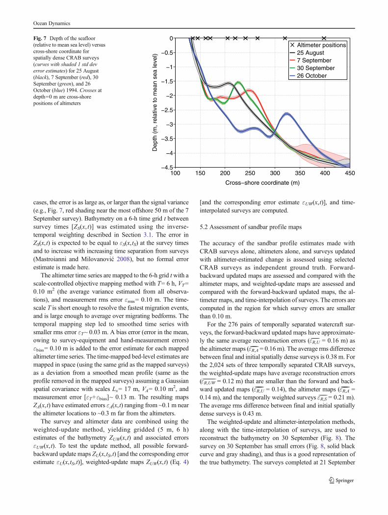
cases, the error is as large as, or larger than the signal variance(e.g., Fig. 7, red shading near the most offshore 50 m of the 7September survey). Bathymetry on a 6-h time grid t betweensurvey times [ZS(x, t)] was estimated using the inverse-temporal weighting described in Section 3.1. The error inZS(x,t) is expected to be equal to εS(x,tS) at the survey timesand to increase with increasing time separation from surveys(Mastroianni and Milovanović 2008), but no formal errorestimate is made here.

The altimeter time series are mapped to the 6-h grid twith ascale-controlled objective mapping method with T= 6 h, VT=0.10 m2 (the average variance estimated from all observa-tions), and measurement rms error εrms= 0.10 m. The time-scale T is short enough to resolve the fastest migration events,and is large enough to average over migrating bedforms. Thetemporal mapping step led to smoothed time series withsmaller rms error εT~ 0.03 m. A bias error (error in the mean,owing to survey-equipment and hand-measurement errors)εbias= 0.10 m is added to the error estimate for each mappedaltimeter time series. The time-mapped bed-level estimates aremapped in space (using the same grid as the mapped surveys)as a deviation from a smoothed mean profile (same as theprofile removed in the mapped surveys) assuming a Gaussianspatial covariance with scales Lx= 17 m, VA= 0.10 m2, andmeasurement error [εT+εbias]~ 0.13 m. The resulting mapsZA(x,t) have estimated errors εA(x,t) ranging from ~0.1 m nearthe altimeter locations to ~0.3 m far from the altimeters.

The survey and altimeter data are combined using theweighted-update method, yielding gridded (5 m, 6 h)estimates of the bathymetry ZUW(x,t) and associated errorsεUW(x,t). To test the update method, all possible forward-backward update maps ZU(x,tS,t) [and the corresponding errorestimate εU(x,tS,t)], weighted-update maps ZUW(x,t) (Eq. 4)

[and the corresponding error estimate εUW(x,t)], and time-interpolated surveys are computed.

5.2 Assessment of sandbar profile maps

The accuracy of the sandbar profile estimates made withCRAB surveys alone, altimeters alone, and surveys updatedwith altimeter-estimated change is assessed using selectedCRAB surveys as independent ground truth. Forward-backward updated maps are assessed and compared with thealtimeter maps, and weighted-update maps are assessed andcompared with the forward-backward updated maps, the al-timeter maps, and time-interpolation of surveys. The errors arecomputed in the region for which survey errors are smallerthan 0.10 m.

For the 276 pairs of temporally separated watercraft sur-veys, the forward-backward updated maps have approximate-ly the same average reconstruction errors (��������εR,U = 0.16 m) asthe altimeter maps (��������εR,A = 0.16m). The average rms differencebetween final and initial spatially dense surveys is 0.38 m. Forthe 2,024 sets of three temporally separated CRAB surveys,the weighted-update maps have average reconstruction errors(� �������������εR,UW = 0.12 m) that are smaller than the forward and back-ward updated maps (��������εR,U = 0.14), the altimeter maps (��������εR,A =0.14 m), and the temporally weighted surveys ��������εR,S = 0.21 m).The average rms difference between final and initial spatiallydense surveys is 0.43 m.

The weighted-update and altimeter-interpolation methods,along with the time-interpolation of surveys, are used toreconstruct the bathymetry on 30 September (Fig. 8). Thesurvey on 30 September has small errors (Fig. 8, solid blackcurve and gray shading), and thus is a good representation ofthe true bathymetry. The surveys completed at 21 September

100 150 200 250 300 350 400 450−4.5

−4

−3.5

−3

−2.5

−2

−1.5

−1

−0.5

0

Dep

th (

m, r

elat

ive

to m

ean

sea

leve

l)

Cross−shore coordinate (m)

Altimeter positions 25 August 7 September 30 September 26 October

Fig. 7 Depth of the seafloor(relative to mean sea level) versuscross-shore coordinate forspatially dense CRAB surveys(curves with shaded 1 std deverror estimates) for 25 August(black), 7 September (red), 30September (green), and 26October (blue) 1994. Crosses atdepth=0 m are cross-shorepositions of altimeters

Ocean Dynamics

(Fig. 8, dashed black curve) and 4 October (Fig. 8, dottedblack curve) are used with altimeter change estimates in theweighted-update method to produce estimates of the bathym-etry (Fig. 8, blue curve) and associated errors (Fig. 8, blueshading). The time-interpolated survey estimate using the 30September and 4 October surveys also is shown (Fig. 8, greencurve), and altimeter interpolation also is used to estimate thebathymetry on 30 September (Fig. 8, red curve) and associat-ed errors (Fig. 8, red shading). The rms reconstruction error(rms difference with the survey on 26 September) for theweighted-update map is 0.08 m [smaller than the averageestimated interpolation error (Eq. 12) 0.25m], for the altimetermaps is 0.12 m (smaller than the average estimated error0.21 m), and for the time-interpolation of surveys is 0.13 m.The rms difference between the surveys on 21 and 30 Sep-tember is 0.16 m, and between the surveys on 30 Septemberand 4 October is 0.14 m.

5.3 Application to sandbar migration

The weighted-update maps improve the temporal resolutionof the evolving cross-shore profile, both during rapid bar-migration events and during times when conditions precludedCRAB surveys (often simultaneous with rapid bar migration)(Fig. 9). Gaussian fits (summed with a linear beach profile) to6-h updated profiles are used as a proxy to determine thesandbar crest position (usually within one or two grid cellsof the location of the maximum of a detrended profile, Figs. 9and 10). Confidence intervals (gray shading in Fig. 10) are

found from the distribution of parameters from a series of fitsto 300 curves generated by summing the updated maps withrandom errors drawn from a Gaussian distribution with stddev given by the estimated mapping rms error. Infrequentdense surveys show the sandbar migrated about 40 m offshorebetween 25 August and 7 September (triangles in Figs. 9 and10). Interpolating between the CRAB surveys assumes themigration was constant in time. However, the updated mapssuggest that the offshoremigration occurred rapidly between 2and 6 September (Fig. 10) during a nor'easter storm [3 msignificant wave height in 8 m depth (Gallagher et al.1998a)], and was preceded by more than 1 week of slowonshore migration (Fig. 10, 25 August to 2 September). Sim-ilarly, during a second nor'easter [14 to 17 October, 4 msignificant wave height in 8 m depth (Gallagher et al.1998a)] the updated maps suggest more rapid migration on15 October than would be inferred from interpolation of theCRAB surveys on 14 and 18 October (Fig. 10). Between 15and 17 October, large waves precluded CRAB surveys of thesandbar.

6 Discussion and summary

Interpolating in time between two spatially dense surveysproduces accurate maps of the seafloor assuming the bathym-etry changes uniformly in time (for some of the rip channelsand some of the bar migration events, e.g., compare greenwith blue curves in Fig. 4). However, surfzone bathymetry

150 200 250 300 350

−0.8

−0.6

−0.4

−0.2

0

0.2

0.4

0.6

0.8

Dep

th (

m, r

elat

ive

to m

ean

prof

ile)

Cross−shore coordinate (m)

offshore

Altimeter positions Survey: 21 September Survey: 4 October Survey: 30 September Altimeters: 30 September Updated: 30 September Survey Interp: 30 September

Fig. 8 Depth of the seafloor (relative to a smoothed mean profile that isremoved from each map) versus cross-shore coordinate from CRABsurveys on 21 September (dashed black curve), 30 September (groundtruth, solid black curve), and 4 October (dotted black curve), and esti-mated for 30 September using the weighted-update (solid blue curve),

altimeter-interpolation (red solid curve), and time-interpolation of the 21September and 4 October CRAB surveys (green solid curve) methods.Shaded areas are 1 std dev error estimates (errors for 21 September and 4October are similar to the gray shading shown for 30 September) and theestimated bathymetries. Crosses show cross-shore positions of altimeters

Ocean Dynamics

often evolves rapidly and non-uniformly when large waves,strong currents, and breaking wave-generated bubbles pre-clude spatially dense bathymetric surveys (e.g., with water-craft), and temporal interpolation is not accurate [e.g., the

migration of the channel (July 21.5 in Fig. 6) and the sandbar(2 to 6 September in Fig. 10) in big waves]. In contrast, fixedaltimeters can estimate bed levels in the presence of largewaves and many bubbles. An array of altimeters sampling

170 190 210 230 250 270 290 310 330

−0.2

0

0.2

0.4

0.6

0.8

1

Dep

th (

m, r

elat

ive

to m

ean

prof

ile)

Cross−shore coordinate (m)

offshore

Altimeter positions Survey: 25 Aug Bar position: 25 Aug Survey: 7 Sep Bar position: 7 Sep Updated maps: 12 hrs Updated map: 2 Sep Bar position: 2 Sep Updated map: 4 Sep Bar position: 4 Sep Updated map: 6 Sep Bar position: 6 Sep

Fig. 9 Depth of seafloor (relative to a smoothed mean profile that isremoved from each map) across the sandbar versus cross-shore coordi-nate (the shoreline is near cross-shore coordinate 100 m). The solid blackcurve is the initial watercraft survey on 25 August 1994, and the dottedblack curve is the survey on 7 September. Gray, red, green, and bluecurves are cross-shore profiles using the weighted-update method every12 h between 25 August and 7 September. The sandbar migrated most

rapidly on 2 September (red curve), through 4 September (green curve),and until 6 September (blue curve).Crosses at depth=1 m are cross-shorepositions of altimeters, and the symbols below the crosses are the bar crestposition (estimated by a fit to a linear slope plus a Gaussian) for surveyson 25 August (upright triangle) and 7 September (inverse triangle) andupdated maps for 2 (red star), 4 (green diamond), and 6 September (bluesquare)

15 Aug 25 Aug 4 Sep 14 Sep 24 Sep 4 Oct 14 Oct 24 Oct

200

250

300

350

400

Cro

ss−

shor

e po

sitio

n (m

)

Date in 1994

offshore

Altimeter positions Surveys Survey: 25 Aug Survey: 7 Sep Updated maps: 12 hrs Updated map: 2 Sep Updated map: 4 Sep Updated map: 6 Sep

Fig. 10 Cross-shore position of the sandbar crest based on altimeter-updated profiles every 3 h (gray curve with shaded 95 % confidenceinterval) and on spatially dense CRAB surveys (black circles andtriangles) versus time. The shoreline is near cross-shore position 100 m.Crosses along the y-axis are cross-shore positions of the altimeters. A

rapid bar migration event (also see Fig. 9) occurred from 2 to 6 Septem-ber, between the surveys on 25 August (upright triangle) and 7 Septem-ber (inverse triangle). The bar cross-shore position moved rapidly startingon 2 September (red star), through 4 September (green diamond), until 6September (blue square)

Ocean Dynamics

continuously can be used to make spatially interpolated bed-level maps at any given time, and may resolve the spatialstructure of the bathymetry with reasonable accuracy if altim-eter spacing is smaller than the spatial decorrelation scales ofthe features of interest. However, altimeter spacing can berelatively sparse and the altimeter bed-level estimates can bebiased. Here, bed-level estimates from spatially dense, butinfrequent surveys were combined with accretion and erosionestimates from spatially sparse, but nearly continuously sam-pling altimeters to form a bathymetric estimate that is moreaccurate than either temporally interpolating between twodense surveys or spatially interpolating between the fixedaltimeters (e.g., Figs. 6 and 10). In studies for which thebathymetric estimate does not need to be independent ofhydrodynamic measurements, additional improvements maybe made by assimilating hydrodynamic measurements(Wilson et al. 2010; Birrien et al. 2013) along with altimeterbed levels or change signals.

The accuracy of the mapped altimeter change (and there-fore of the updated maps) and of the mapped altimeter bedlevels is sensitive to the trend removed from the observationsprior to mapping (and subsequently added back to the mappedestimate), owing to the tendency of objectively mapped esti-mates to approach zero far from information (Rybicki andPress 1992, also see Appendix). This tendency can beexploited to improve accuracy where there is insufficientinformation. Here, the mapped altimeter bed levels far frominstrument locations approached a mean beach slope (for therip channels) or a smoothed mean profile (for the sandbars).The mean slope and smoothed mean profile were found usingthe dense survey data, so the altimeter bed-level estimates arenot strictly independent of the dense surveys. For the maps ofbed-level change from altimeters used in the update method,no mean or trend was removed, and thus the estimated changeis zero far from altimeters. There are alternatives that may bemore appropriate in other applications, such as allowing thechange signal estimate far from sensors to approach the aver-age change.

Although interpolation weights estimated assuming spa-tially uniform and temporally constant Gaussian covariancefunctions produced relatively accurate seafloor maps, the pat-terns of the estimated mapping errors and the errors found inthe reconstruction tests did not agree, perhaps because thebathymetry evolves more rapidly and with larger amplitudenear the shore and when waves are large. Choosing spatiallyand temporally variable covariance functions may producemore accurate bathymetric and error estimates. Further inves-tigation of the sensitivity of the estimated and reconstructionerrors to the covariance estimates is needed to guide theselection of interpolation weights.

Here, the observations of changes in bed level at thelocations of fixed altimeters were mapped and added tomaps made from occasional spatially dense surveys. When

multiple dense surveys were available, updated maps madefrom each survey were combined in a weighted average.For evolving dredged channels and natural sandbars in thesurf zone, the updated maps are a better estimate of thebathymetry than maps made by spatially interpolating al-timeter estimates of the bed level or by temporally inter-polating dense surveys.

Acknowledgments The US Army Corps of Engineers Field ResearchFacility (Duck, NC, USA) provided excellent logistical support for boththe 1994 and 2012 datasets.We thank Brian Scarborough and Jason Pipesfor driving the landing craft and making depressions in the surfzoneseafloor, and Jesse McNinch and the FRF team for their generous hospi-tality. We also thank Bill Boyd, David Clark, Danik Forsman, DanaGiffen, Levi Gorrell, Jeff Hansen, Julia Hopkins, Sean Kilgallin, ChristenRivera-Erick, Jenna Walker, Anna Wargula, Regina Yopak, and SethZippel for their tenacity in the field. Peter Traykovski and Fred Jaffredesigned and built the WHOI altimeters. Falk Feddersen, EdithGallagher, Robert Guza, Thomas Herbers, the Scripps Center for CoastalStudies field crew, and many others helped gather the Duck94 data. Thiswork was funded by the Office of the Assistant Secretary of Defense forResearch and Engineering, a National Defense Science and EngineeringGraduate Fellowship, A National Science Foundation Graduate ResearchFellowship, the National Science Foundation, and the Office of NavalResearch.

Appendix: Interpolation and mapping of irregularlysampled observations

Often, a set of bed-level observations z(xj,yj,tj), where xj and yjare the cross- and alongshore coordinates of the jth observa-tion made at time tj, are mapped using linear interpolation to aregular spatial (xi,yi) and temporal (ti) grid:

Z xi; yi; tið Þ ¼Xj

W ijz x j; y j; t j� �

ð6Þ

where Z is the linearly interpolated bed-level elevation esti-mate at a set of “mapping coordinates” (xi,yi,ti) and Wij is theweight of the jth observation at the ith mapping coordinate.

One common choice of interpolation weights is inverseseparation weighting, e.g., in time:

Wij ¼ A ti−t j�� ��−1 ð7Þ

The factor A (which may be a function of the observationand mapping coordinates) is sometimes set such that the onlyobservations with nonzero weights are those immediatelypreceding and following the mapping coordinate, and maybe normalized by the sum of the weights such that weights ateach mapping coordinate sum to one.

Other mapping methods take advantage of knowledge ofthe signal covariance to seek an estimate of the bathymetrythat minimizes the root-mean-square (rms) difference between

Ocean Dynamics

the true and the mapped bathymetry (Bretherton et al. 1976).Optimal weights are:

Wij ¼Xj0

Pj0 j� �−1

Rj0i ð8Þ

where Pj 'j is the covariance between observed elevations atlocations with indices j' and j, Rj 'i is the covariance betweenobserved and mapped elevations, and [ ]−1 is the matrixinverse. This method is referred to as objective mapping oroptimal interpolation. Often a Gaussian model for the covari-ance is used for mapping either in space or in time, e.g., in onedimension:

Rmn ¼ Vexp −pm−pnð Þ22L2

!ð9Þ

where V is the estimated signal variance, p is the spatial or timecoordinate, m and n are arbitrary indices, and L is adecorrelation length or time scale. The covariance betweenall observed elevations is:

Pj0 j ¼ Rj0 j þ ε2O xj; y j; t j� �

δ j0 j ð10Þ

where εO(xj,yj,tj) is the rms observational error associatedwiththe jth observation. It is assumed that observation errors areuncorrelated with errors at other locations and times (the deltafunction δj 'j=0 if j '≠j,and δj 'j=1 if j '=j).

Often a mean or trend M is removed before mapping andthen added back in after mapping (this can be considered ascale separation):

Z xi; yi; tið Þ ¼Xj

W ij z x j; y j; t j� �

−Mh i

þM ð11Þ

The functionMmay be an estimate of the true signal mean,a linear trend, a higher-order trend, or an ensemble-averagedestimate of a mean state. The choice becomes particularlyimportant for data that are under-sampled because far fromobservations the interpolation weights tend to approach zero,and thus the bathymetric estimate approachesM (Rybicki andPress 1992).

The estimated interpolation error is:

ε xi; yi; tið Þ ¼ V−Xj

W ijRij ð12Þ

If there are small-scale features (e.g., ripples, megaripples,cusps) that are not resolved by the surveys (e.g., there isaliasing owing to undersampling) or are not desired in theestimate of the bathymetry (e.g., considered noise), weightsmay be derived to minimize the rms difference between themapped bathymetry and a filtered (e.g., smoothed) true ba-thymetry (Ooyama 1987; Plant et al. 1999). When seeking the

optimal estimate of smoothed bathymetry, smoothed covari-ance functions of the true bathymetry (Ooyama 1987) areused. Here, the covariance function is assumed to be a Gauss-ian (Eq. 10) with the scale L set to the smoothing scale (aresolvable scale of interest) and the signal variance V set to theestimated variance of the smoothed bathymetry. In the pres-ence of unresolved scales, εO should include both the rmsmeasurement error and an rms estimate of the error associatedwith unresolved scales (e.g., the rms amplitude of bedforms).The results are optimal only if the covariance function ischosen correctly (e.g., a spatially variable covariance functioncould be used), but more detailed information about the truebathymetry would be needed to improve the covariance func-tion estimate, and it is expected that the interpolation errors arenot highly sensitive to errors in the choice of covariancefunction (Rybicki and Press 1992).

References

AustinM, Scott T, Brown J, Brown J,MacMahan J,MasselinkG, RussellP (2010) Temporal observations of rip current circulation on amacro-tidal beach. Cont Shelf Res 30:1149–1165. doi:10.1016/j.csr.2010.03.005

Birkemeier WA, Mason C (1984) The CRAB: A unique nearshoresurveying vehicle. J Surv Eng 110(1):1–7. doi:10.1061/(ASCE)0733-9453(1984)110:1(1)

Birkemeier WA, Long C, Hathaway K (2001) DELILAH, DUCK94 &SandyDuck: Three Nearshore Field Experiments. Coast Eng ProcASCE 1(25):4052–4065. doi:10.9753/icce.v25

Birrien F, Castelle B, Marieu V, Dubarbier B (2013) On a data-modelassimilation method to inverse wave-dominated beach bathymetryusing heterogeneous video-derived observations. Ocean Eng 73:126–138. doi:10.1016/j.oceaneng.2013.08.002

Bretherton FP, Davis RE, Fandry CB (1976) A technique for objectiveanalysis and design of oceanographic experiments applied toMODE-73. Deep-Sea Res 23:559–582. doi:10.1016/0011-7471(76)90001-2

Chen Q, Dalrymple R, Kirby J, Kennedy A, Haller M (1999) Boussinesqmodeling of a rip current system. J Geophys Res 104(C9):20617–20637. doi:10.1029/1999JC900154

Dalrymple R, MacMahan J, Reniers A, Nelko V (2011) Rip currents.Annu Rev Fluid Mech 43:551–581. doi:10.1146/annurev-fluid-122109-160733

Dugan J, Morris W, Vierra K, Piotrowski C, Farruggia G, Campion D(2001) Jetski-based nearshore bathymetric and current survey sys-tem. J Coast Res 17(4):900–908

Elgar S, Gallagher EL, Guza RT (2001) Nearshore sandbar migra-tion. J Geophys Res 106:11623–11627. doi:10.1029/2000jc000389

Falqués A, Coco G, Huntley DA (2000) A mechanism for the generationof wave-driven rhythmic patterns in the surf zone. J Geophys Res105(C10):24071–24088. doi:10.1029/2000JC900100

Feddersen F, Gallagher EL, Guza RT, Elgar S (2003) The dragcoefficient, bottom roughness, and wave breaking in the near-shore. Coast Eng 48:189–195. doi:10.1016/s0378-3839(03)00026-7

Gallagher E, BoydW, Elgar S, Guza R,WoodwardB (1996) Performanceof a sonar altimeter in the nearshore. Mar Geol 133:241–248. doi:10.1016/0025-3227(96)00018-7

Ocean Dynamics

Gallagher E, Elgar S, Guza R (1998a) Observations of sand bar evolutionon a natural beach. J Geophys Res 103:3203–3215. doi:10.1029/97JC02765

Gallagher E, Elgar S, Thornton E (1998b) Megaripple migration in anatural surfzone. Nature 394:165–168. doi:10.1038/28139

Gallagher EL, Elgar S, Guza RT, Thornton EB (2005) Estimating near-shore bedform amplitudes with altimeters. Mar Geol 216(1):51–57.doi:10.1016/j.margeo.2005.01.005

Gallop SL, Bryan KR, Coco G, Stephens SA (2011) Storm-driven chang-es in rip channel patterns on an embayed beach. Geomorphology127:179–188. doi:10.1016/j.geomorph.2010.12.014

Garnier R, Falqués A, Calvete D, Thiébot J, Ribas F (2013) Amechanismfor sandbar straightening by oblique wave incidence. Geophys ResLett 40. doi:10.1002/grl.50464

Genton MG (2007) Separable approximations of space-time covariancematrices. Environmetrics 18(7):681–695. doi:10.1002/env.854

Haller M, Dalrymple R, Svendsen I (2002) Experimental study of near-shore dynamics on a barred beach with rip channels. J Geophys Res107(C6):3061. doi:10.1029/2001JC000955

Henderson S, Allen J, Newberger P (2004) Nearshore sandbar migrationpredicted by an eddy-diffusive boundary layer model. J GeophysRes 109. doi:10.1029/2003JC002137

Hoefel F, Elgar S (2003) Wave-induced sediment transport and sandbarmigration. Science 299:1885–1887. doi:10.1126/science.1081448

Holland KT, Holman RA, Lippmann TC, Stanley J, Plant N (1997)Practical use of video imagery in nearshore oceanographicfield studies. IEEE J Ocean Eng 22:81–92. doi:10.1109/48.557542

Holman RA, Haller MC (2013) Remote sensing of the nearshore. AnnRev Mar Sci 5(1):95–113. doi:10.1146/annurev-marine-121211-172408

Holman RA, Sallenger AH, Lippmann TC, Haines JW (1993) Theapplication of video image processing to the study of nearshoreprocesses. Oceanography 6:78–85. doi:10.5670/oceanog.1993.02

Holman RA, Symonds G, Thornton EB, Ranasinghe R (2006) Ripspacing and persistence on an embayed beach. J Geophys Res111:C01006. doi:10.1029/2005JC002965

Holman R, Plant N, Holland T (2013) cBathy: a robust algorithm forestimating nearshore bathymetry. J Geophys Res 118:2595–2609.doi:10.1002/jgrc.20199

Hsu T-J, Elgar S, Guza R (2006) Wave-induced sediment transport andonshore sandbar migration. Coast Eng 53:817–824. doi:10.1016/j.coastaleng.2006.04.003

Kuik A, van Vledder G, Holthuijsen L (1988) A method for the routineanalysis of pitch-and-roll buoy wave data. J Phys Oceanogr 18:1020–1034. doi:10.1175/1520-0485(1988)018<1020:AMFTRA>2.0.CO;2

Lippmann T, Holman R (1989) Quantification of sand-bar morphology: avideo technique based on wave dissipation. J Geophys Res 94(C1):995–1011. doi:10.1029/JC094iC01p00995

Lippmann T, Smith G (2008) Shallow surveying in hazardous waters.Shallow Water Survey Conf, Durham, NH, USA

MacMahan J (2001) Hydrographic surveying from personal watercraft. JSurv Eng 127(1):12–24. doi:10.1061/(ASCE)0733-9453(2001)127:1(12)

MacMahan J, Thornton E, Reniers A (2006) Rip current review. CoastEng 53:191–208. doi:10.1016/j.coastaleng.2005.10.009

Mastroianni G, Milovanović GV (2008) Interpolation processes: basictheory and applications. Springer, Berlin. doi:10.1007/978-3-540-68349-0

Moulton M, Elgar S, Raubenheimer B (2013) Structure and evolution ofdredged rip channels. Proc of Coastal Dynamics ’13, ASCE,Arcachon, Fr. 1263–1274

Ooyama KV (1987) Scale-controlled objective analysis. Mon WeatherRev 115:2479–2506. doi :10 .1175/1520-0493(1987)115<2479:SCOA>2.0.CO;2

Plant NG, Holman RA, Freilich MH (1999) A simple model for interan-nual sandbar behavior. J Geophys Res 104(C7):15755–15776. doi:10.1029/1999JC900112

Plant NG, Holland KT, Puleo JA (2002) Analysis of the scale errors innearshore bathymetric data. Mar Geol 191:71–86. doi:10.1016/S0025-3227(02)00497-8

Plant NG, Edwards K, Kaihatu J, Veeramony J, Hsu L, Holland K (2009)The effect of bathymetric filtering on nearshore process modelresults. Coast Eng 56:484–493. doi:10.1016/j.coastaleng.2008.10.010

Ruessink BG, van Enckevork IMJ, Kingston KS, Davidson MA (2000)Analysis of observed two- and three-dimensional nearshore barbehavior. Mar Geol 169:161–183. doi:10.1016/S0025-3227(00)00060-8

Rybicki GB, Press WH (1992) Interpolation, realization, and reconstruc-tion of noisy, irregularly sampled data. Astrophys J 398:169–176

Thornton E, Humiston R, Birkemeier W (1996) Bar/trough generation ona natural beach. J Geophys Res 101(C5):12097–12110. doi:10.1029/96JC00209

van Dongeren A, Plant N, Cohen A, Roelvink D, Haller MC, Catalán P(2008) Beach Wizard: nearshore bathymetry estimation throughassimilation of model computations and remote observations.Coastal Eng 55(12):1016–1027. doi:10.1016/j.coastaleng.2008.04.011

van Enckevort IMJ, Ruessink BG (2003) Video observations of nearshorebar behaviour. Part 2: alongshore non-uniform variability.Continental Shelf Res 23:513–532. doi:10.1016/S0278-4343(02)00235-2

van Enckevort IMJ, Ruessink BG, Coco G, Suzuki K, Turner IL, PlantNG, Holman RA (2004) Observations of nearshore crescentic sand-bars. J Geophys Res 109, C06028. doi:10.1029/2003JC002214

Wilson GW, Özkan-Haller HT, Holman RA (2010) Data assimilation andbathymetric inversion in a two-dimensional horizontal surf zonemodel. J Geophys Res 115, C12057. doi:10.1029/2010JC006286

Ocean Dynamics