Australian Bathymetry and Topography Grid · PDF fileIn previous Australian bathymetry grids single beam has been included particularly for ... Australian Bathymetry and Topography

G E O S C I E N C E A U S T R A L I A

T.G. Whiteway

APPLYING GEOSCIENCE TO AUSTR ALIA’S MOST IMPORTANT CHALLENGES

Record

2009/21

Australian Bathymetry and Topography Grid June 2009

GeoCat # 67703

Australian Bathymetry and Topography Grid, June 2009 GEOSCIENCE AUSTRALIA RECORD 2009/21 by T.G. Whiteway1

1. Petroleum and Marine Division, Geoscience Australia, GPO Box 378, Canberra ACT 2601

Department of Industry, Tourism & Resources Minister for Resources, Energy & Tourism: The Hon. Martin Ferguson, AM, MP Secretary: Mr John Pierce Geoscience Australia Chief Executive Officer: Dr Neil Williams,PSM © Commonwealth of Australia, 2009 This work is copyright. Apart from any fair dealings for the purpose of study, research, criticism, or review, as permitted under the Copyright Act 1968, no part may be reproduced by any process without written permission. Copyright is the responsibility of the Chief Executive Officer, Geoscience Australia. Requests and enquiries should be directed to the Chief Executive Officer, Geoscience Australia, GPO Box 378 Canberra ACT 2601. Geoscience Australia has tried to make the information in this product as accurate as possible. However, it does not guarantee that the information is totally accurate or complete. Therefore, you should not solely rely on this information when making a commercial decision. ISSN 1448-2177 ISBN 978-1-921498-89-3 web ISBN 978-1-921498-89-6 DVD ISBN 978-1-921498-84-8 hardcopy GeoCat # 67703 Bibliographic reference: Whiteway, T.G., 2009. Australian Bathymetry and Topography Grid, June 2009. Geoscience Australia Record 2009/21. 46pp.

Australian Bathymetry and Topography Grid – June 2009

Table of Contents TABLE OF CONTENTS III

1. ABSTRACT 1

IMPORTANT INFORMATION 1

2. INTRODUCTION 2

3. INPUT DATASETS 3

SINGLE BEAM DATA 3 MULTIBEAM (SWATH) BATHYMETRY 4 DIGITAL BATHYMETRY FROM NATMAP 1:250,000 SERIES AND AHS FAIRSHEETS 4 LASER AIRBORNE DEPTH SOUNDER 5 SATELLITE MEASUREMENTS – ETOPOV2G AND ETOPO1 5 AUSTRALIAN TOPOGRAPHY 6 NEW ZEALAND TOPOGRAHY 6 SRTM DEM 6 CHRISMAS, COCOS AND LORD HOWE ISLAND BATHYMETRIC GRIDS 7 GRID FOR THE GULF OF PAPUA AND ADJACENT AREAS 7

4. THE PROCESS 9

STEP 1 – AREA OF INTEREST 12 STEP 2 – DATA PREPARATION 12 STEP 3 – IMPORT DATA INTO INTREPID™ DATABASES BASED ON TILES 13 STEP 4 – CREATE TILE GRIDS, CLIP AND MERGE TILED GRIDS INTO A SINGLE GRID 14 STEP 5 – CLEANING SURVEYS GRID 16 STEP 6 – FILLING ON-SHELF ZONES AND HOLES 16 STEP 7 – MOSAICING ALL GRIDS 17 STEP 8 – CLEANING THE MOSAICED GRID 17 STEP 9 – FINAL ADDITIONS 18 STEP 10 – FINAL CLEANING PROCESS 18 STEP 11 – FINAL PREPARATION OF PRODUCTS 18

5. FINAL PRODUCTS 19

2009 BATHYMETRIC GRID OF AUSTRALIA 19 LINEAGE SHAPEFILE 23

6. 2005 AND 2009 BATHYMETRIC GRIDS – A COMPARISON 24

NEW DATA 24 REVISED ETOPO DATA 28 INTERPOLATION ARTEFACTS 29 METHEDOLOGY ARTEFACTS 32 ERRANEOUS DATA 34

7. CONCLUSION 37

8. ACKNOWLEDGMENTS 38

iii


9. REFERENCES 38

10. OTHER DATA SOURCES 39

APPENDIX 1 – MULTIBEAM SURVEYS 40

APPENDIX 2 – SRTM DEM METADATA 46

iv


1

1. Abstract In 2005 Geoscience Australia and the National Oceans Office undertook a joint project to produce a consistent, high-quality 9 arc second (0.0025° or ~250m at the equator) bathymetric grid for Australian waters. In 2009 a number of new datasets were included in an updated version of the grid. The 2009 bathymetric grid of Australia has been produced to include recently acquired datasets, and solutions to issues identified in the previous version. The revised grid has the same extents as its 2005 counterpart, including the Australian water column jurisdiction lying between 92˚ E and 172˚ E, and 8˚ S and 60˚ S. The waters adjacent to the continent of Australia and Tasmania are included, as are areas surrounding Macquarie Island, and the Australian Territories of Norfolk Island, Christmas Island, and Cocos (Keeling) Islands. The area selected does not include Australia's marine jurisdiction offshore from the Territory of Heard and McDonald Islands and the Australian Antarctic Territory. This report details the datasets and procedures used to produce the 2009 bathymetric grid of Australia. As per the 2005 grid, the 0.0025 decimal degree (dd) resolution is only supported where direct bathymetric observations are sufficiently dense (e.g. where swath bathymetry data or digitised chart data exist) (Webster and Petkovic, 2005). In areas where no sounding data are available (in waters off the Australian shelf), the grid is based on the 2 arc minute ETOPO (Smith and Sandwell, 1997) and 1 arc minute ETOPO (Amante and Eakins, 2008) satellite derived bathymetry. The topographic data (on shore data) is based on the revised Australian 0.0025dd topography grid (Geoscience Australia, 2008), the 0.0025dd NZ topography grid (Geographx, 2008) and the 90m SRTM DEM (Jarvis et al, 2008). The final dataset has been provided in ESRI grid and ER Mapper (ers) formats. An associated shapefile has been produced so that the user can identify the input datasets that were used in the final grid.

IMPORTANT INFORMATION

This grid is not suitable for use as an aid to navigation, or to replace any products produced by the Australian Hydrographic Service. Geoscience Australia produces the 0.0025dd bathymetric grid of Australia specifically to provide regional and local broad scale context for scientific and industry projects, and public education. The 0.0025dd grid size is, in many regions of this grid, far in excess of the optimal grid size for some of the input data used. On parts of the continental shelf it may be possible to produce grids at higher resolution, especially where LADS or multibeam surveys exist. However these surveys typically only cover small areas and hence do not warrant the production a regional scale grid at less than 0.0025dd. There are a number of bathymetric datasets that have not been included in this grid for various reasons. Comments or queries about the data included in the grid (or excluded) can be directed to: [email protected].

mailto:[email protected]


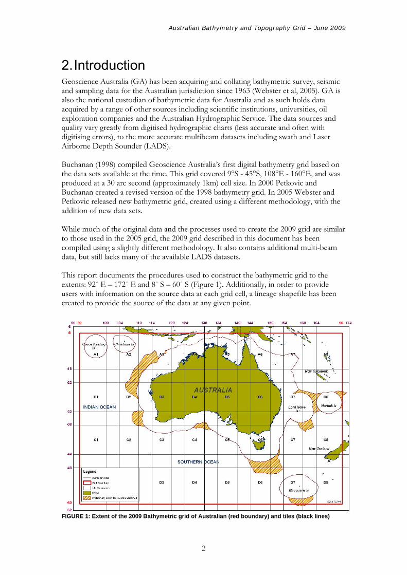
2. Introduction Geoscience Australia (GA) has been acquiring and collating bathymetric survey, seismic and sampling data for the Australian jurisdiction since 1963 (Webster et al, 2005). GA is also the national custodian of bathymetric data for Australia and as such holds data acquired by a range of other sources including scientific institutions, universities, oil exploration companies and the Australian Hydrographic Service. The data sources and quality vary greatly from digitised hydrographic charts (less accurate and often with digitising errors), to the more accurate multibeam datasets including swath and Laser Airborne Depth Sounder (LADS). Buchanan (1998) compiled Geoscience Australia’s first digital bathymetry grid based on the data sets available at the time. This grid covered 9°S - 45°S, 108°E - 160°E, and was produced at a 30 arc second (approximately 1km) cell size. In 2000 Petkovic and Buchanan created a revised version of the 1998 bathymetry grid. In 2005 Webster and Petkovic released new bathymetric grid, created using a different methodology, with the addition of new data sets. While much of the original data and the processes used to create the 2009 grid are similar to those used in the 2005 grid, the 2009 grid described in this document has been compiled using a slightly different methodology. It also contains additional multi-beam data, but still lacks many of the available LADS datasets. This report documents the procedures used to construct the bathymetric grid to the extents: 92˚ E – 172˚ E and 8˚ S – 60˚ S (Figure 1). Additionally, in order to provide users with information on the source data at each grid cell, a lineage shapefile has been created to provide the source of the data at any given point.

FIGURE 1: Extent of the 2009 Bathymetric grid of Australian (red boundary) and tiles (black lines)

2


3. Input Datasets The following text describes each dataset used in the production of the 2009 grid. The input datasets used to create the final grid varied greatly in resolution, source and data type. In this revised version of the Australian bathymetry grid the following datasets were used:

• Multibeam • Fairsheets and 1:250,000 Series • Laser Airborne Depth Sounder (LADS) (Only those LADS datasets that had

previously been converted from LAT were used in this grid) • Satellite altimetry measurements – ETOPO2v2g • Australian topography • New Zealand topography • SRTM DEM

Single beam datasets were not used in the creation of the 2009 grid (see below). All datasets once gridded were shifted to ensure cell alignment matched the Australian DEM prior to mosaicing to ensure the accuracy of the Australian DEM was maintained. Methodologies used in these processes are outlined in Part 4.

SINGLE BEAM DATA

Measurements of water depth particularly in deep oceans were nearly impossible to gather prior to the development of echosounder tools. Echosounders are a form of active sonar that create a sound (or ping) that is bounced off the ocean floor. On the ping’s return, the transducer (antenna) receives the signal and based on the speed of return and the known speed of sound through the water column, the water depth is calculated. Single beam echo sounders collect bathymetry data along a ships path (often referred to as ship track data). In previous Australian bathymetry grids single beam has been included particularly for areas of deep ocean where there are limited other sources of data. In the 2009 grid, the single beam dataset was considered for inclusion, but was not used due to issues emerging from its use in previous grids, specifically:

• The inclusion of single beam data in previous grids has resulted in lines/stripes of high resolution data running through the lower resolution ETOPO data. This causes artefacts that look like channels and ridges running through the grid

• There are also issues associated with the quality of the raw data. These include: - levelling and historic navigation issues which means the data is often

inaccurate, and; - limited time available to clean the data, which means ‘dirty’ areas of data

in the single beam datasets still exist. Additionally, a majority of the single beam data covers the shelf. In the majority of shelf areas, there are better quality datasets available including multibeam and LADS that can be used to produce a more accurate and consistent grid. The compliment of issues surrounding the use of the single beam data has led to its exclusion from the 2009 version of the grid.

3


MULTIBEAM (SWATH) BATHYMETRY

Multibeam echosounders map the seabed using a ‘fan-shaped swath’ of sonar beams. This allows for large areas of seabed to be mapped in a relatively short time, making them a more efficient tool than single beam echosounders. Multibeam or swath datasets are an extremely valuable source of bathymetric data, providing highly accurate broad coverage for both on and off shelf areas. As the national custodian for bathymetric data, GA holds data from government organisations, academic and foreign institution multi-beam survey data. Appendix 1 lists the swath surveys used in this grid (Figure 5). All GA swath datasets are initially cleaned in CARIS HIPS/SIPS software and are exported as xyz files for use in gridding packages. The swath datasets used in this grid have not been decimated or averaged prior to gridding.

DIGITAL BATHYMETRY FROM NATMAP 1:250,000 SERIES AND AHS FAIRSHEETS

The following section has been extracted from Webster and Petkovic (2005). “In 1994, GA received a set of charts from the Australian Hydrographic Service, Royal Australian Navy (AHS), sourced from the NATMAP 1:250,000 bathymetric series. These charts included contours on the face of the map and soundings as spot depths on the back. The spot depths for a subset of the charts, mainly for the NW Shelf and Gulf of Carpentaria, were captured digitally by the AHS, and these data were provided to GA. The digitisation of the remainder of the charts was continued by GA and completed in 2001. At the request of GA, the AHS provided an additional set of charts as scanned images for the shelf in selected regions. These 'fairsheets' displayed hand-written spot depths for surveys completed over various periods of time. To save costs the fairsheets were digitised selectively, leaving out near coastal data points, and, as a general rule, digitising lines to a minimum spacing of 2 nautical miles (~3.7 km). Some charts of high interest to clients were digitised in entirety. There are 1049 charts in the collection.” These raw datasets have been collected in a range of different Datums, and due to time constraints many of these have not been converted back to a single datum (MSL). The raw data points are stored in GA’s Oracle database and can be extracted by location as required.

4


LASER AIRBORNE DEPTH SOUNDER

The following section has been extracted from Webster and Petkovic (2005). “The AHS has been operating its Laser Airborne Depth Sounder (LADS) systems since 1993. The system uses red and green laser light emitted from a stabilised platform inside a fixed wing aircraft. The light pulses reflected from the sea surface (red) and sea floor (green) are separately detected, and the time difference between the sea surface and sea floor returns allows calculation of the water depth. Data are typically acquired at a rate of 900 soundings in a 240 m wide x 5 m long swath per second. The system works best in clean water of the pristine coral reefs of the Coral Sea down to 70m depth. Shallower maximum depths are achieved in other areas, such as Great Barrier Reef, Bass Strait, Timor Sea (40-50m), South Australia (30-35m), Torres Strait (15-25m), and anywhere waters are not clear.” The LADS data is of particular importance to the large scale 0.0025° bathymetry grid because;

• it fills the area between the coastline (Australian DEM) and the offshore datasets such as swath, and

• it provides excellent edge boundaries for reefs, coastlines and islands. “AHS provided GA with LADS data around Australia, including 1773 LADS datasets. In order to be included in the gridding process, each dataset needed to be converted from HTF format into XYZ, be datum converted from LAT to MSL and, each dataset needed to be imported into Intrepid™ as an Intrepid™ database. Due to time constraints only the LADS data used previously in the 2005 Australian bathymetry grid was used for this grid. The LADS datasets used included data from Queensland waters particularly around the Great Barrier Reef.” Only limited LADS datasets were used in the production of the 2009 grid due to the limited coverage they provide, and lack of conversion time and storage available to convert these datasets from the LAT to MSL Datum.

SATELLITE MEASUREMENTS – ETOPOV2G AND ETOPO1

The 2 arc minute ETOPO2v2g (U.S. Department of Commerce, 2006) data based on predicted bathymetry from satellite altimetry (Smith and Sandwell, 1997) was used as base data for the grid where more accurate data sources were not available (i.e. for much of the deep ocean). In 2008 during development of the revised Australian bathymetric grid, a 1 arc minute version of ETOPO, ETOPO1 (Amante and Eakins, 2008) was released. In the Australian region, this dataset is based primarily on GEBCO estimated Seafloor bathymetry. It was used as a late inclusion to replace data in the top left of the Australian bathymetry grid where both he Australian, and ETOPO2v2g data were inaccurate. The ETOPO grids were resampled to 0.0025dd using a bilinear conversion as the nearest neighbour method created grid artefacts including striations. In the 2009 version of the grid the ETOPO data appears to be less smooth and less detailed than the ETOPO data in the 2005 bathymetry grid. In the 2005 bathymetry grid the ETOPO data was re-

5


interpolated in Intrepid, in the 2009 version there was no interpolation in order to keep the values consistent with those produced in the original ETOPO data. This predicted bathymetry (Figure 2) was included in areas where the high-resolution data (swath and digitised charts) were not available, and was not used on the Australian shelf. All other datasets were mosaiced on top of the ETOPO data. The predicted bathymetry contributes the characteristic artefact of rippled noise which has a wavelength of about 25km and amplitude of about 200m in the deep water.

AUSTRALIAN TOPOGRAPHY

The Australian 9" DEM (Geoscience Australia, 2008) (Figure 3) was used as the topographic dataset for the Australian Continent and surrounding islands. This is GA’s 4th edition DEM and has been calculated using ANUDEM v 5.2.2.

FIGURE 2: ETOPO2v2g (U.S. Department of Commerce, 2006)

NEW ZEALAND TOPOGRAHY

The 250m New Zealand DEM was sourced from Geographx (NZ) Ltd (2008) in Ascii format, non-projected, NZ Mercator datum (Figure 3). The projection of this dataset was modified to WGS84 and, as with the Australian DEM, was then directly mosaiced over the other datasets without feathering or smoothing.

SRTM DEM

The 90m Shuttle Radar Topography Mission (SRTM) DEM (Figure 3) was sourced for the southern areas of Papua New Guinea and Indonesia from the CGIAR Consortium

6


for Spatial Information (CIGAR-CSI) in the WGS84 datum in the ASCII format. The individual datasets were mosaiced and then resampled to 0.0025dd using ArcGIS nearest neighbour method, and values below 0m were removed so that only land based values were used. The SRTM data was then directly mosaiced over the other datasets without feathering or smoothing.

FIGURE 3: Australian (GA, 2008), NZ (Geographx, 2008) and SRTM (Jervis et al., 2008) Digital Elevation Models (DEM’s) used in the production of the 2009 bathymetric grid of Australia

CHRISMAS, COCOS AND LORD HOWE ISLAND BATHYMETRIC GRIDS

For the Christmas, Cocos and Lord Howe Islands, bathymetric grids had been produced with hand edited data. Fledermaus with the 3D editor were used to compare input data points, and points not consistent with the higher accuracy datasets (swath and LADS) were deleted prior to gridding. The island datasets have been gridded in Intrepid and have been incorporated into the revised bathymetry grid to improve accuracy in these regions.

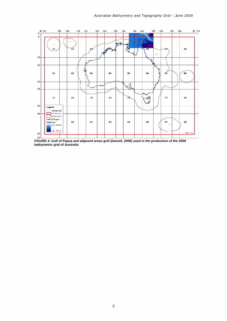
GRID FOR THE GULF OF PAPUA AND ADJACENT AREAS

The grid in the region of the Gulf of Papua (Figure 4) was created using a combination of processes from GMT (Generic Mapping Tools) to average the input data points and ANUDEM to grid the final product (Daniell, 2008). The Gulf of Papua grid comprises the following input datasets:

• Multibeam sonar • Australian Hydrographic Service (AHS) Fair sheet and survey data • Ship Track and Miscellaneous data (including external surveys) • SRTM • Landsat derived Bathymetry

7


FIGURE 4: Gulf of Papua and adjacent areas grid (Daniell, 2008) used in the production of the 2009 bathymetric grid of Australia

8


4. The Process A number of programs were used to create the 2009 revised Australian bathymetry grid, in particular:

• ArcGIS for review of gridded data, mosaicing without feathering and the creation of the lineage shapefile.

• ER Mapper for gridding replacement data in problem areas, and for data review. • Intrepid™ for initial raw data editing for Fairsheets, gridding and mosaicing with

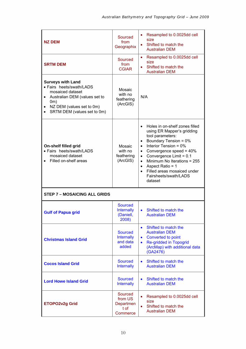
feathering. The process used to develop the grid is summarised in Table 1, which defines an eleven step sequence. Table 1 – Summary of steps and processes used to create the 2009 bathymetric grid

STEP / INTERIM GRID PROCESSES

ANALYSIS TYPE

INPUT PARAMETERS

STEP 1 – AREA OF INTEREST

STEP 2 – DATA PREPARATION

STEP 3 – IMPORT DATA INTO INTREPID™ DATABASES

STEP 4 – CREATE TILE GRIDS, CLIP AND MERGE TILED GRIDS INTO A SINGLE GRID

Surveys grid LADS Swath Fairsheets with AHD Datum Fairsheets with Non-AHD

datums Fairsheets with Unknown

datums Reef s lines

Gridded together

(Intrepid™) Tiles

clipped and mosaiced in ArcGIS

Cell Size = 0.0025 Minimum Curvature tension =

0.5 Maximum Iterations = 100 Maximum Residual = 1.0 m Extrapolation = 10 cells Additional Smoothing = No Initial Cell Assignment =

Nearest Neighbour Output Precision =

IEEE4ByteReal

STEP 5 – CLEANING SURVEY GRIDS

Surveys grid cleaned Cleaned in ER Mapper

Erroneous data set to null using region editing

STEP 6 – FILLING ON-SHELF ZONES AND HOLES

Australian DEM Sourced Internally

9


NZ DEM Sourced

from Geographix

Resampled to 0.0025dd cell size

Shifted to match the Australian DEM

SRTM DEM Sourced

from CGIAR



Surveys with Land Fairs heets/swath/LADS

mosaiced dataset Australian DEM (values set to

0m) NZ DEM (values set to 0m) SRTM DEM (values set to 0m)

Mosaic with no

feathering (ArcGIS)

N/A

On-shelf filled grid Fairs heets/swath/LADS

mosaiced dataset Filled on-shelf areas

Mosaic with no

feathering (ArcGIS)

Holes in on-shelf zones filled using ER Mapper’s gridding tool parameters:

Boundary Tension = 0% Interior Tension = 0% Convergence speed = 40% Convergence Limit = 0.1 Minimum No Iterations = 255 Aspect Ratio = 1 Filled areas mosaiced under

Fairsheets/swath/LADS dataset

STEP 7 – MOSAICING ALL GRIDS

Gulf of Papua grid

Sourced Internally (Daniell, 2008)


Christmas Island Grid

Sourced Internally and data

added


Converted to point Re-gridded in Topogrid

(ArcMap) with additional data (GA2476)

Cocos Island Grid Sourced Internally


Lord Howe Island Grid Sourced Internally


ETOPO2v2g Grid

Sourced from US

Department of

Commerce



10


Higher accuracy grid Gulf of Papua grid Christmas, Cocos and Lord

Howe Island grids On-shelf filled

Mosaic with no

feathering (ArcGIS)

N/A

Higher accuracy and ETOPO2v2g Higher accuracy grid ETOPO2v2g

Mosaic with no

feathering (ArcGIS)

N/A

High resolution/ETOPO2v2g and Land Australi an DEM NZ DEM SRTM

Mosaic with no

feathering (ArcGIS)

N/A

STEP 8 – CLEANING MOSAICED GRID

Cleaned grid High resolution/ETOPO2v2g and

Land

Cleaned in ER Mapper


Holes filled using ER Mapper’s gridding tool parameters:

Boundary Tension = 0% Interior Tension = 0% Convergence speed = 40% Convergence Limit = 0.1 Minimum No Iterations = 255 Aspect Ratio = 1

Cleaned mosaiced grid High resolution/ETOPO2v2g and

Land cleaned Fill areas

Mosaic with no

feathering (ArcGIS)

N/A

STEP 9 – FINAL ADDITIONS

Final Additions Cleaned mosaiced grid GA2476 leg 3 GA2447 GA2413

Mosaic with no

feathering (ArcGIS)

N/A

STEP 10 – CLEANING FINAL ADDIITIONS GRID

ETOPO1 Grid

Sourced from US

Department of

Commerce



11


Addition of ETOPO1 data Final Additions grid

Mosaic with no

feathering (ArcGIS)

N/A

Cleaned grid Final Additions grid

Cleaned in ER Mapper


Holes filled using ER Mapper’s gridding tool parameters:

Boundary Tension = 0% Interior Tension = 0% Convergence speed = 40% Convergence Limit = 0.1 Minimum No Iterations = 255 Aspect Ratio = 1

Cleaned mosaiced final grid Final Additions Grid Fill areas

Mosaic with no

feathering (ArcGIS)

N/A

STEP 11 – FINAL PREPARATION OF PRODUCTS

Integer grid Integer

(ArcGIS)

Grid values set to integer, as the cell size and data quality does not support sub-metre accuracy

Clipped grid Clip

(ArcGIS) Grid clipped to final extents

(9°S - 45°S, 108°E - 160°E)

STEP 1 – AREA OF INTEREST

The Area of Interest was defined to match the 2005 Bathymetry grid. Two degrees were added to each edge of the grid and removed at the end of processing to reduce edge effects. In figure 1 the outer red boundary represents the final outer boundary of the grid. The initial grids were interpolated to the outer black boundary prior to clipping.

AOI extents: 92, 172, -8, -60 Extended AOI extents: 90, 174, -6, -62

STEP 2 – DATA PREPARATION

Raw Data

Raw data points used in this grid included swath, fairsheets and LADS datasets. Due to the large extent of raw data and limited computing capacity, the area of interest was divided into 32 tiles, 14 degrees wide by 11 degrees long, with 4 degrees of overlap (trimmed before merging). All raw datasets were converted to XYZ files from the

12


database (in tiles as represented in figure 1), and each input dataset was exported to XYZ format on a tile by tile basis.

ETOPO2v2g

ETOPO2v2g has a cell size of 0.033dd. In order to incorporate the data into the bathymetry grid the data was resampled to a 0.0025dd cell size using bilinear interpolation in ArcGIS. The bilinear interpolation process interpolates the new values of each smaller cell using a bilinear function. Original values of the ETOPO2v2g data have not been preserved, as a result.

ETOPO1

ETOPO1 has a cell size of 0.0167dd. In order to incorporate the data into the bathymetry grid the data was resampled to a 0.0025dd cell size using bilinear interpolation in ArcGIS. The bilinear interpolation process interpolates the new values of each smaller cell using a bilinear function. Original values of the ETOPO2v2g data have not been preserved, as a result.

Australian Topography

The Australian topography grid required no conversions and was used as the base grid to which all other grid were shifted to maintain a single cell configuration throughout the processing.

New Zealand Topography

The projection of this dataset was modified from NZ Mercator datum to WGS84. Values below 0m were removed so that only land based values were used.

SRTM DEM

The SRTM data was downloaded as individual blocks of data. These datasets were mosaiced and then resampled from a cell size of 0.00083dd to 0.0025dd using ArcGIS nearest neighbour method. Values below 0m were removed so that only land based values were used.

Christmas, Cocos and Lord Howe Island Bathymetric grids

The Christmas, Cocos and Lord Howe Island Bathymetric grids required no conversions.

Gulf of Papua and Adjacent Areas Bathymetric grid

The Gulf of Papua and Adjacent Areas Bathymetric grid required no conversions.

STEP 3 – IMPORT DATA INTO INTREPID™ DATABASES BASED ON TILES

Each raw XYZ file was imported into an Intrepid™ database using WGS84 datum with geodetic projection. Intrepid was chosen because it is widely used within GA as a geophysical processing tool, and the gridding tool allows considerable flexibility of parameter control, grid masking, and auxiliary operations such as stitching, merging and editing (Billings and Fitzgerald, 1998).

13


STEP 4 – CREATE TILE GRIDS, CLIP AND MERGE TILED GRIDS INTO A SINGLE GRID

Gridding

The datasets gridded in this process included: • Multibeam – swath • Fairsheets with AHD Datum • Fairsheets with Non-AHD datums • Fairsheets with Unknown datums • LADS

The multibeam, fairsheet and LADS datasets were gridded together to minimise the propagation of edge effects where the different datasets meet. The grids were computed using Intrepid software, which requires data to be present in an Intrepid database or set of databases. “Intrepid was chosen because of its ease of use with large datasets, its combination of GUI and batch operation, fine control over parameter setting, large user base within the organisation, associated grid manipulation utilities, and mature version history. To create the present grid Intrepid was used in batch mode accessing several databases sequentially. These same databases can be updated as the need requires, and grids of any specification can be created from them. Intrepid was originally designed to deal with potential field data, and uses the minimum curvature algorithm which is not well suited to topography. Other software such as that of Hutchinson (1989) deals effectively with stream-lines and roughness, for example, but doesn’t allow masking, which is essential to the present task. In order to simulate the roughness of topographic character in Intrepid, the minimum curvature tension parameter was set to mid-way between pure minimum curvature and pure minimum potential. This avoids some of the over-shoot that results from minimum curvature surface fitting in areas of poor control, while at the same time doesn’t produce severe cusps at data points. Inspection of test grids indicates that this compromise setting gives sufficiently smooth results yet retains some of the characteristic roughness of topographic data. Billings and Fitzgerald (1998) discuss some of Intrepid’s gridding options and its limitations. The main gridding parameters are given in the table below.” (Webster and Petkovic, 2005)

14


Table 2 - Gridding parameter settings for Intrepid

Parameter Value Latitude range 8° S – 60° S

Longitude range 92° E – 172° E Cell size 0.0025° (9”)

Minimum curvature tension 0.5 Maximum iterations 100 Maximum residual 1.0 m

Extrapolation 10 cells (~1.5 km) Setting no-data areas to null Yes

Additional Smoothing No Initial cell assignment nearest neighbour

Output precision IEEE4ByteReal

Clip and Mosaic

Each grid was clipped in ArcGIS to remove the 2 degrees of excess (or 4 degrees of overlap) per tile. The final clipped grids were then mosaiced together using the ‘mosaic to new raster’ function in ArcGIS (Table 1). This is a direct overlay process with no feathering or smoothing used to produce a grid of the entire area (figure 5). The final grid mosaiced in this process is from here on called the ‘surveys grid’.

FIGURE 5: Surveys grid

15


STEP 5 – CLEANING SURVEYS GRID

All grids created from raw data had data errors that required editing or removal. In the case of Fairsheet data there were a number of digitising errors (in the raw data) that were identified after the first gridding process. These included extreme low and high points in areas of gentle slope. The erroneous points identified were checked against the original Fairsheets (which have previously been scanned and rectified). Where a digitising error was confirmed, the point was corrected (through editing in Intrepid™) prior to gridding, and the Australian Hydrographic Office was sent the x, y and z coordinates of any digitising errors for review. In all other datasets the raw data was not modified due to the dataset size. The size of the datasets meant that editing program (Intrepid™) could not handle the datasets without regular crashing. Therefore, inaccurate data areas identified in any dataset (including some unresolved areas in the Fairsheets) were removed from the grided datasets using a clip process. The removal of inaccurate data was undertaken in two steps:

1. For each grid the areas where data values were less than -9999m depth or greater than 1000m were set to null.

2. For each dataset a vector file (ER Mapper) of data errors to be removed was created, and used to clip out errors using the region set to null.

STEP 6 – FILLING ON-SHELF ZONES AND HOLES

In the on-shelf zone of Australia, and in some off-shelf areas, the data was dense enough that there were only small holes with no data coverage. In initial versions of the bathymetric grid, the ETOPO data was mosaiced behind the greater accuracy datasets to fill these gaps. However, in many cases the ETOPO data was vastly different to the higher quality data and caused spurious holes or ridges. Consequently in this version of the grid, areas where on-shelf gaps occurred were filled with data interpolated in ER Mapper™. In previous versions there have also been issues caused by filling holes through interpolation that are connected to land areas. When ER Mapper interpolates between high land values and low ocean values the interpolation can create areas where ocean values are higher than the land. In order to minimise these issues in this version of the grid, all values of the land grids (including Australia, SRTM and New Zealand) were set to 0m. These grids were then mosaiced (with no feathering) into the swath/LADS/fairsheets combination to set a value of 0m on the coast. An interpolation process was then run to fill the gaps between the sea values and land values. The use of this process creates a secondary artefact in that there will always be a smooth interpolation from ocean values to the land (i.e.) deep water drop offs may be removed. However, this process does remove the occurrence of land values (i.e. > 0m) in the ocean area. The collection of data along the coast (both land and ocean) is vitally important to reduce errors in this part of the grid for future products.

16


A number of interpolation methods and input parameters were trialled including tin to raster and topo to raster in ArcGIS, Intrepid’s nearest neighbour interpolation and ER Mapper’s tin and minimum curvature interpolation techniques. The process selected was minimum curvature interpolation in ER Mapper. This process was able to grid large datasets effectively and created fewer artefacts than many other interpolation options. A number of parameters for the minimum curvature technique were also trialled. The final parameters chosen minimised the tension requirements while ensuring that the tension was great enough to prevent the data from fluctuating wildly, as per the ER Mapper default values.

• Boundary Tension = 0% • Interior Tension = 0% • Convergence speed = 40% • Convergence Limit = 0.1 • Minimum No Iterations = 255 • Aspect Ration = 1

The Minimum Curvature interpolation process re-interpolates all input data. Consequently the data from the interpolated grids was used to fill the holes only.

STEP 7 – MOSAICING ALL GRIDS

Grids were mosaiced with the highest accuracy grids on top and the lowest accuracy on the bottom. All grids were shifted prior to mosaicing to match the Australian DEM to ensure that both major products released from Geoscience Australia have common topography. Note that as a result the NZ DEM and SRTM DEM datasets will have been shifted slightly and will not line up perfectly with their original location. In this grid the Gulf of Papua, Lord Howe, Christmas Island, ETOPO2v2g and Cocos Island grids were mosaiced with the surveys grid with a feathering process to reduce edge effects. The feathering process smooths the edges so that one grid mosaics with another grid without the large steps seen when no feathering is applied. The feathering process has been minimised so that only cells adjacent to the joins are feathered. The parameters used were:

• Overlap limit = 20m • Filter length = 2500m • Smoothing iterations = 100 • Smoothing residual = 1

All other grids (New Zealand Digital Elevation Models, the SRTM DEM) were mosaiced without feathering. These grids were directly overlaid with no smoothing to retain cliff lines and their original data values. If smoothing were undertaken on the DEM, cliff edges would be smoothed as part of the process.

STEP 8 – CLEANING THE MOSAICED GRID

Following the completion of a mosaiced version of the bathymetry grid, a number of edge effects and flaws in theof data required editing. These areas of data were located and set to no-data using region identification in ER Mapper. The holes created were then

17


interpolated using the ER Mapper Gridding tool (with parameters as set in Step 7) and these fill areas were mosaiced with no feathering.

STEP 9 – FINAL ADDITIONS

On completion of the grid three additional datasets were identified that needed to be added. These datasets (GA2413, GA2477 and GA2476 – Leg3) were mosaiced into the final dataset without feathering in ArcGIS.

STEP 10 – FINAL CLEANING PROCESS

Following addition of new datasets a final version of cleaning was undertaken to ensure that there were no remaining edge effects or errors. The cleaning process was undertaken as per those outlined in Step 7. Additionally in this step the top left section of the grid was removed and replaced with ETOPO1. ETOPO1 is a newly released version of ETOPO data that has higher accuracy, including data in regions plagued by poor data in ETOPOv2g. This data was used to fill areas where both swath and ETOPO2v2g datasets had inaccuracies.

STEP 11 – FINAL PREPARATION OF PRODUCTS

The final version of the bathymetry grid was converted to an integer grid as the 0.0025dd resolution and source accuracy of the data does not support higher accuracy. This version was then clipped to the required extent and projected to WGS84. The final 9” grid was then re-produced in ER Mapper, ESRI grid and ASCII XYZ formats.

18


5. Final Products 2009 BATHYMETRIC GRID OF AUSTRALIA

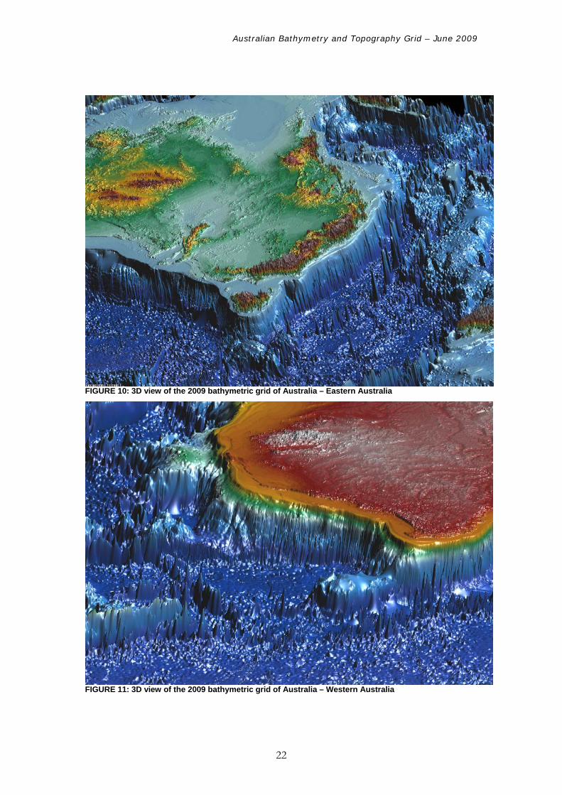
The 2009 bathymetric grid of Australia has been produced for modelling, visualisation and map presentation (Figure 6 through 11). Each dataset was gridded at 0.0025dd without smoothing, and overlayed with the best accuracy grids (swath) on top, and the least accurate (ETOPO) grid at the bottom (without feathering).The terrain models for Australia, New Zealand and Indonesia / Papua New Guinea have been directly overlaid with no smoothing to retain the raw data for each grid.

FIGURE 6: 2009 bathymetric grid of Australia

19


FIGURE 7: 2009 bathymetric grid of Australia - Queensland

FIGURE 8: 2009 bathymetric grid of Australia – north-west Australia

20


21

FIGURE 9: 3D view of the 2009 bathymetric grid of Australia – Western Australia


22

FIGURE 11: 3D view of the 2009 bathymetric grid of Australia – Western Australia

FIGURE 10: 3D view of the 2009 bathymetric grid of Australia – Eastern Australia


LINEAGE SHAPEFILE

An associated dataset, the lineage shapefile, was created to show the source input datasets for each part of the final grid (Figure 12). The shapefile was created by converting each grid to an integer grid, and mosaicing these in the same order as the grids were mosaiced to produce the 2009 bathymetry grid. The mosaiced grid was then exported to shapefile. Note that there has been a smoothing process applied to the edges of the swath, fairsheets, LADS and around the island grids to allow for streamlined gradient between each data type. As such the areas where edges of each different dataset meet will not exactly replicate the original data sources in these locations.

FIGURE 12: Lineage shapefile for the 2009 bathymetric grid of Australia

23


6. 2005 and 2009 Bathymetric Grids – A Comparison

In creating a revised bathymetric grid, a number of requirements were met. The following outlines the differences between the 2005 and 2009 bathymetric grids of Australia, particularly focussing on the required outcomes for the 2009 grid.

NEW DATA

The 2009 grid incorporates a number of new datasets where available. In particular a number of new Swath datasets were included as illustrated in figures 13 and 14. However no new LADS datasets were included in this grid due to time constraints.

a.

b.

FIGURE 13: Addition of Swath data off the East Australian shelf in the 2009 grid (b) (2005 grid (a))

24


a.

b.

FIGURE 14: Addition of Swath data from Survey GA 2476 in the 2009 grid (b) (2005 grid (a))

25


A range of improved DEMS were also used in the creation of this grid. The latest DEMs including the new 2008 Australian DEM, the SRTM DEM (figure 15b) and the 250m New Zealand DEM were resampled to match the cell size of the Australian DEM, and were mosaiced directly over the final dataset to give continuity and improved land data accuracy.

a.

b.

FIGURE 15: Inclusion of high quality DEMs increased the overall quality as seen with the inclusion of the SRTM DEM in the Indonesian area in the 2009 grid (b) (2005 grid (a))

26


Additionally, a number of higher accuracy bathymetric datasets were also incorporated. Grids produced in separate processes for the Lord Howe Island (figure 16), Gulf of Papua and Christmas Island were a vast improvement on previous grids of these areas. The new datasets were directly overlaid to provide higher quality data for these areas.

a.

b.

FIGURE 16: Addition of a higher accuracy grids in the 2009 grid (b), including the Lord Howe Island grid in the image above, increased the overall quality (2005 grid (a))

27


REVISED ETOPO DATA

ETOPO2v2g and ETOPO1 datasets were used as background datasets in the 2009 version of the bathymetric grid of Australia. In the 2005 grid the ETOPO data was resampled to a 0.0025dd cell size using an interpolation process that smoothed the data and added apparent detail (figure 17a). In the 2009 grid the ETOPO data was resampled to 0.0025dd using a bilinear process to minimise interpolation. This means that the ETOPO data in the 2009 grid is coarser and seems to have less detail. However it is more true to its original source (figure 17).

a.

b.

FIGURE 17: The ETOPO data in the 2005 (a) grid is much smoother and appears to show more detail than the 2009 (b) grid as it has been interpolated using a different method.

28


INTERPOLATION ARTEFACTS

In the 2005 grid a number of coastline interpolation artefacts appeared particularly along the Queensland coastline (figures 18 and 19). In the 2009 grid, coastal bathymetry data was interpolated to meet a DEM with a flat height of 0m. This forced the interpolation to maintain an even rise, minimising interpolation artefacts around the coastline.

a.

b.

FIGURE 18: Removal of interpolation artefacts in the 2009 grid (b) (2005 grid (a))

29


a.

b.

FIGURE 19: Removal of interpolation artefacts in the 2009 grid (b) (2005 grid (a))

30


There were also areas in the 2005 grid where interpolation processes had been used on the Australian DEM, causing smoothing of the final terrain data (figure 20). These interpolation artefacts were removed by directly overlaying the DEM data for each terrain over the bathymetry data.

a.

b.

FIGURE 20: Removal of interpolation errors over the DEM from the 2005 grid (a) (2009 grid (b))

31


METHEDOLOGY ARTEFACTS

When two different quality datasets are gridded together and one has higher values than the other (effects of positional accuracy, depth accuracy, datum issues etc) the interpolation package will interpolate to make the edges of the grids meet. Therefore highs will drop off quickly to meet low values and vice versa (figure 21a).

a.

b.

FIGURE 21: The interpolation process for the 2005 grid (a) in many cases produced a longed (less sharp) boundary between the different data types compared to mosaicing and feathering method used in the 2009 grid (b). In the 2009 grid a different process was applied to allow the production of a shapefile showing the general input dataset for each of the grid cells. The process involved

32


gridding like accuracy datasets in the same process, and feather mosaicing them with other datasets that had been gridded together. This differed from previous grids where all datasets were gridded together. For this reason, there are smoothing artefacts around sections of data that were mosaiced, similar to those seen when all datasets are interpolated together (figure 21b). However, in the 2009 grid, in some areas they will appear sharper, as the boundary change distance has been minimised to avoid smoothing through other higher accuracy datasets.

33


ERRANEOUS DATA

A range of errors including irregular ship track lines, Swath spikes, ETOPO gravity anomaly highs and Fairsheets digitising errors were identified in the 2005 grid. Generally these errors are products of the raw data, causing high and low anomalies (figure 22), lines of erroneous data (figure 23) and large scale interpolation artefacts (figure 24). Where identified these errors were removed through editing the output grid. However, the en mass errors seen in the single beam data meant that this entire dataset was removed prior to interpolation.

a.

b.

FIGURE 22: Removal of spurious highs and lows seen in the 2005 grid (a) (2009 grid (b))

34


a.

b.

FIGURE 23: Removal of ship track errors seen in the 2005 grid (a) (2009 grid (b))

35


a.

b.

FIGURE 24: Removal of data processing errors seen in the 2005 grid (a) (2009 grid (b))

36


7. Conclusion The 2009 iteration of the bathymetric grid has addressed a range of issues seen in the 2005 version, and has included a number of new datasets. The production of an associated lineage file provides users with an indication of the source of the raw data. The 2009 bathymetry grid provides excellent regional context, and the greater volume of higher accuracy data on the shelf provides an improving local context. However, the production of an Australian region bathymetric grid should be seen as an iterative process of review and re-compilation to fully exploit the latest methods for managing and gridding new data.

37


8. Acknowledgments The following people provided advice, data and information during the process: Mike Sexton, Cameron Mitchell, Cameron Buchanan, Peter Milligan, Murray Woods, Mark Webster, Andrea Cortese, James Daniell, Michael Morse, Peter Petkovic, George Bernadel and Richard Mileczko.

9. References Amante, C. and B. W. Eakins, ETOPO1 1 Arc-Minute Global Relief Model: Procedures, Data Sources and Analysis, National Geophysical Data Center, NESDIS, NOAA, U.S. Department of Commerce, Boulder, CO, August 2008. Billings, S.D. and D.J. FitzGerald, 1998. An integrated framework for interpolating airborne geophysical data with special reference to radiometrics. Exploration Geophysics, 29, 284-289. Buchanan, C., 1998. 30 arc second gridded bathymetry. GA - Geoscience Australia, CD-ROM. Carroll, D., (ed), 1996. Geodata 9 second DEM user guide. Australian Surveying & Land Information Group, Canberra. Daniell, J. J., 2008. Development of a bathymetric grid for the Gulf of Papua and adjacent areas: A note describing its development, J. Geophys. Res., 113, F01S15, doi:10.1029/2006JF000673. Geographx, 2008. New Zealand 250m Digital Elevation Model, available from http://www.geographx.co.nz/downloads.html Geoscience Australia, 2008. GEODATA 9 Second DEM and D8, Version 3 and Flow Direction Grid 2008, Data User Guide, Canberra, Australia, available from http://www.ga.gov.au/nmd/products/digidat/dem_9s.jsp Jarvis A., H.I. Reuter, A. Nelson, E. Guevara, 2008. Hole-filled seamless SRTM data V4, International Centre for Tropical Agriculture (CIAT), available from http://srtm.csi.cgiar.org. Petkovic, P. and C. Buchanan, 2002. Australian bathymetry and topography grid (January 2002). [CDROM]. Canberra: Geoscience Australia. Smith, W. H. F., and D. T. Sandwell, 1997. Global seafloor topography from satellite altimetry and ship depth soundings, Science, v. 277, p. 1957-1962, 26 Sept., 1997. Webster, M.A., and P. Petkovic, 2005. Australian Bathymetry and Topography Grid, June 2005. Record 2005/12.

38

http://www.geographx.co.nz/downloads.html

http://www.ga.gov.au/nmd/products/digidat/dem_9s.jsp

http://srtm.csi.cgiar.org/


10. Other Data Sources ETOPOv2g

U.S. Department of Commerce National Oceanic and Atmospheric Administration National Environmental Satellite, Data, and Information Service National Geophysical Data Centre http://www.ngdc.noaa.gov/mgg/fliers/06mgg01.html

ETOPO1

U.S. Department of Commerce National Oceanic and Atmospheric Administration National Environmental Satellite, Data, and Information Service National Geophysical Data Centre http://www.ngdc.noaa.gov/mgg/global/global.html

NZ 250m DEM

Geographx The Dominican Observatory 34 Slamanca Rd Kelburn Wellington New Zealand http://www.geographx.co.nz/downloads.html

SRTM 90m DEM

CGIAR Consortium for Spatial Information http://srtm.csi.cgiar.org/

COCOS, CHRISTMAS AND LORD HOWE ISLAND BATHYMETRIC GRIDS

R. Mleczko Risk and Impact Analysis Group Geoscience Australia GPO Box 378, Canberra, ACT, 2601

GULF OF PAPUA AND ADJACENT AREAS GRID

J. Daniell Seabed Mapping and Characterisation Group Marine Geoscience and Environment Group Geoscience Australia GPO Box 378, Canberra, ACT, 2601

39

http://www.ngdc.noaa.gov/mgg/fliers/06mgg01.html

http://www.ngdc.noaa.gov/mgg/global/global.html

http://www.geographx.co.nz/downloads.html

http://srtm.csi.cgiar.org/


40

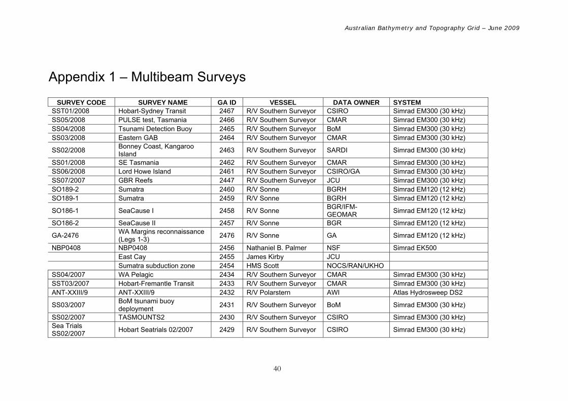
Appendix 1 – Multibeam Surveys

SURVEY CODE SURVEY NAME GA ID VESSEL DATA OWNER SYSTEM SST01/2008 Hobart-Sydney Transit 2467 R/V Southern Surveyor CSIRO Simrad EM300 (30 kHz) SS05/2008 PULSE test, Tasmania 2466 R/V Southern Surveyor CMAR Simrad EM300 (30 kHz) SS04/2008 Tsunami Detection Buoy 2465 R/V Southern Surveyor BoM Simrad EM300 (30 kHz) SS03/2008 Eastern GAB 2464 R/V Southern Surveyor CMAR Simrad EM300 (30 kHz)

SS02/2008 Bonney Coast, Kangaroo Island 2463 R/V Southern Surveyor SARDI Simrad EM300 (30 kHz)

SS01/2008 SE Tasmania 2462 R/V Southern Surveyor CMAR Simrad EM300 (30 kHz) SS06/2008 Lord Howe Island 2461 R/V Southern Surveyor CSIRO/GA Simrad EM300 (30 kHz) SS07/2007 GBR Reefs 2447 R/V Southern Surveyor JCU Simrad EM300 (30 kHz) SO189-2 Sumatra 2460 R/V Sonne BGRH Simrad EM120 (12 kHz) SO189-1 Sumatra 2459 R/V Sonne BGRH Simrad EM120 (12 kHz)

SO186-1 SeaCause I 2458 R/V Sonne BGR/IFM-GEOMAR Simrad EM120 (12 kHz)

SO186-2 SeaCause II 2457 R/V Sonne BGR Simrad EM120 (12 kHz)

GA-2476 WA Margins reconnaissance (Legs 1-3) 2476 R/V Sonne GA Simrad EM120 (12 kHz)

NBP0408 NBP0408 2456 Nathaniel B. Palmer NSF Simrad EK500 East Cay 2455 James Kirby JCU Sumatra subduction zone 2454 HMS Scott NOCS/RAN/UKHO SS04/2007 WA Pelagic 2434 R/V Southern Surveyor CMAR Simrad EM300 (30 kHz) SST03/2007 Hobart-Fremantle Transit 2433 R/V Southern Surveyor CMAR Simrad EM300 (30 kHz) ANT-XXIII/9 ANT-XXIII/9 2432 R/V Polarstern AWI Atlas Hydrosweep DS2

SS03/2007 BoM tsunami buoy deployment 2431 R/V Southern Surveyor BoM Simrad EM300 (30 kHz)

SS02/2007 TASMOUNTS2 2430 R/V Southern Surveyor CSIRO Simrad EM300 (30 kHz) Sea Trials SS02/2007 Hobart Seatrials 02/2007 2429 R/V Southern Surveyor CSIRO Simrad EM300 (30 kHz)


SO-94 SO-94 2428 R/V Sonne IFM GEOMAR Atlas Hydrosweep DS SO-113_2 SO-113 L2 2427 R/V Sonne IFM GEOMAR Atlas Hydrosweep DS KR9813 KR9813 2426 R/V Kairei JAMSTEC SST02/2007 Lacepede Shelf 2425 R/V Southern Surveyor GA Simrad EM300 (30 kHz) SS01/2007 Bight Basin 2424 R/V Southern Surveyor GA Simrad EM300 (30 kHz) SST01/2007 SSTransit 01/2007 2423 R/V Southern Surveyor GA/CSIRO Simrad EM300 (30 kHz) YK01-15 YK01-15 2422 S/V Yokosuka JAMSTEC Seabeam 2112 (12 kHz) YK01-14 YK01-14 2421 S/V Yokosuka JAMSTEC Seabeam 2112 (12 kHz) YK02-07 YK02-07 2420 S/V Yokosuka JAMSTEC Seabeam 2112 (12 kHz) SO-190Transit SO-190T 2418 R/V Sonne IFM GEOMAR Simrad EM-120 (12 kHz) SS09/2006 LHRIDGE 2416 R/V Southern Surveyor UNSW Simrad EM300 (30 kHz) SS11/2006 Tasmounts1 2415 R/V Southern Surveyor CMAR/DEH Simrad EM300 (30 kHz) SST03/2006 SSTransit03/2006 2414 R/V Southern Surveyor GA Simrad EM300 (30 kHz) SS10/2006 NSW Slopes 2413 R/V Southern Surveyor GA Simrad EM300 (30 kHz) MR04-01 MR04-01 2412 R/V Mirai JAMSTEC Seabeam 2112 (12 kHz) SST02/2006 SSTransit 02/2006 2411 R/V Southern Surveyor UNSW Simrad EM300 (30 kHz) SST01/2006 SSTransit 01/2006 2409 R/V Southern Surveyor GA Simrad EM300 (30 kHz) SS06/2006 Rowley Shoals 2408 R/V Southern Surveyor GA Simrad EM300 (30 kHz) SS05/2006 Meso_Eddies 2406 R/V Southern Surveyor UWA Simrad EM300 (30 kHz) MR03K04L5 MR03K04_Leg5 2405 R/V Mirai JAMSTEC Seabeam 2112 (12 kHz) NBP0501 NBP0501 2404 R/V Nathaniel B Palmer NSF Simrad EM-120 (12 kHz) SS03/2006 TRULL06 2402 R/V Southern Surveyor UTAS Simrad EM300 (30 kHz) Hobart Trials 2401 R/V Southern Surveyor CSIRO Simrad EM300 (30 kHz) SS04/2006 Leeuwin Currents 2400 R/V Southern Surveyor UWA Simrad EM300 (30 kHz) J.K_11/04 2399 James Kirby JCU Reson Seabat 8101 MOGAM06 2398 R/V OGS Explora OGS Reson Seabat 8150 (12 kHz) SS02/2006 Palaeo Murrays 2397 R/V Southern Surveyor ANU Simrad EM300 (30 kHz) VT82 (MD153L2?) AUSFAIR_GAB Transit 2396 R/V Marion Dufresne IPEV Thompson Marconi TSM 5265 MD153 AUSFAIR_ZoNeco12 2395 R/V Marion Dufresne IPEV Thompson Marconi TSM 5265 MD152 TAS-NZ Transit 2394 R/V Marion Dufresne IPEV Thompson Marconi TSM 5265 MR04K03L2 MR04K03_Leg2 2393 R/V Mirai JAMSTEC Seabeam 2112 (12 kHz)

41


EW9510 EW9510 2392 R/V Maurice Ewing LDEO Thompson Marconi TSM 5265 EW0002 EW0002 2391 R/V Maurice Ewing LDEO Thompson Marconi TSM 5265 SS10/2005 Wabio_2 2390 R/V Southern Surveyor CSIRO Simrad EM300 (30 kHz)

NBP0406 NBP0406 2389 R/V Nathaniel B Palmer US Antarctic Program Simrad EM-120 (12 kHz)

MR00K07L2 MR00K07_Leg2 2388 R/V Mirai JAMSTEC Seabeam 2112 (12 kHz) MR01K05L2 MR01K05_Leg2 2387 R/V Mirai JAMSTEC Seabeam 2112 (12 kHz) MR02K04L2 MR02K04_Leg2 2386 R/V Mirai JAMSTEC Seabeam 2112 (12 kHz) MR03K03L2 MR03K03_Leg2 2385 R/V Mirai JAMSTEC Seabeam 2112 (12 kHz) MR03K04L1 MR03K04_Leg1 2384 R/V Mirai JAMSTEC Seabeam 2112 (12 kHz) SS09/2005 Naturaliste Rocks 2383 R/V Southern Surveyor UWA Simrad EM300 (30 kHz) MD148 PECTEN 2382 R/V Marion Dufresne SydneyUni/IPEV Thompson Marconi TSM 5265 SWS2003 2381 Conference Dataset Various SS06/2005 Cornea-Cartier 2375 R/V Southern Surveyor AIMS/ANU Simrad EM300 (30 kHz) MANAUTE MANAUTE 2374 N.O. L'Atalante IFREMER Simrad EM-12D (12 kHz) Sydney Woolongong Transit 2373 HMAS Melville RAN Atlas-Fansweep (20 -100) VANC29MV VANC29 2372 R/V Melville SIO Seabeam 2000 (12 kHz) VANC25MV VANC25 2371 R/V Melville SIO Seabeam 2000 (12 kHz) VANC22MV VANC22 2370 R/V Melville SIO Seabeam 2000 (12 kHz) VANC21MV VANC21 2369 R/V Melville SIO Seabeam 2000 (12 kHz) VANC15MV VANC15 2368 R/V Melville SIO Seabeam 2000 (12 kHz) EW0112 EW0112 2367 R/V Ewing LDEO Atlas Hydrosweep EW9910 EW9910 2364 R/V Ewing LDEO Atlas Hydrosweep SS09/2004 SS200409 2363 R/V Southern Surveyor Uni of Sydney Simrad EM300 (30 kHz) Topas Trials 2361 R/V Southern Surveyor GA Simrad EM300 (30 kHz) SS11/2004 Notove 2360 R/V Southern Surveyor ANU Simrad EM300 (30 kHz) SS10/2004 N_Fiji_1 2359 R/V Southern Surveyor UTAS Simrad EM300 (30 kHz) SS07/2004 WinterEnv 2358 R/V Southern Surveyor CSIRO Simrad EM300 (30 kHz) SS06/2004 Cotrove 2357 R/V Southern Surveyor ANU Simrad EM300 (30 kHz) Sydney Hobart Transit 2356 R/V Southern Surveyor CSIRO Simrad EM300 (30 kHz) SS04/2004 S E Ecosystems 2355 R/V Southern Surveyor CSIRO Simrad EM300 (30 kHz)

42


EM300 Trials 2354 R/V Southern Surveyor CSIRO Simrad EM300 (30 kHz) BHP_HIRES 2353 BHPP Rottnest 2352 HMAS Cook RAN-JCU Seabeam (12 kHz) Albany 2351 HMAS Cook RAN-JCU Seabeam (12 kHz) Adelaide 2350 HMAS Cook RAN-JCU Seabeam (12 kHz) Eaxa 2349 HMAS Cook RAN-JCU Seabeam (12 kHz) GBR 2348 HMAS Cook RAN-JCU Seabeam (12 kHz) ASHMORE 2347 HMAS Leeuwin RAN Atlas-Fansweep (20 -100) AUSTREA3 AUSTREA3 2346 N.O. L'Atalante LINZ/IFREMER Simrad EM-12D (12 kHz) VANC30MV VANC30 2343 R/V Melville SIO Seabeam 2000 (12 kHz) VANC28MV VANC28 2342 R/V Melville SIO Seabeam 2000 (12 kHz) VANC27MV VANC27 2341 R/V Melville SIO Seabeam 2000 (12 kHz) VANC26MV VANC26 2340 R/V Melville SIO Seabeam 2000 (12 kHz) VANC24MV VANC24 2339 R/V Melville SIO Seabeam 2000 (12 kHz) VANC23MV VANC23 2338 R/V Melville SIO Seabeam 2000 (12 kHz) VANC20MV VANC20 2337 R/V Melville SIO Seabeam 2000 (12 kHz) VANC19MV VANC19 2336 R/V Melville SIO Seabeam 2000 (12 kHz) VANC16MV VANC16 2333 R/V Melville SIO Seabeam 2000 (12 kHz) VANC14MV VANC14 2332 R/V Melville SIO Seabeam 2000 (12 kHz) VANC12MV VANC12 2331 R/V Melville SIO Seabeam 2000 (12 kHz) VANC11MV VANC11 2330 R/V Melville SIO Seabeam 2000 (12 kHz) VANC10MV VANC10 2329 R/V Melville SIO Seabeam 2000 (12 kHz) NBP0209 NBP0209 2328 R/V Nathaniel B Palmer NSF Simrad EM-120 (12 kHz) NBP0008 NBP0008 2327 R/V Nathaniel B Palmer NSF Seabeam 2112 (12kHz) NBP9603a NBP9603a 2326 R/V Nathaniel B Palmer NSF Seabeam 2112 (12kHz) EW0003 EW0003 2325 R/V Ewing LDEO Atlas Hydrosweep EW9914 EW9914 2324 R/V Ewing LDEO Atlas Hydrosweep EW9912 EW9912 2323 R/V Ewing LDEO Atlas Hydrosweep EW9911 EW9911 2322 R/V Ewing LDEO Atlas Hydrosweep EW9512 EW9512 2321 R/V Ewing LDEO Atlas Hydrosweep EW9511 EW9511 2320 R/V Ewing LDEO Atlas Hydrosweep

43


TAN0308 NORFANZ 2312 R/V R/V Tangaroa NIWA Simrad EM-300 (30 kHz) MR03K04L6 MR03K04_Leg6 2309 R/V Mirai JAMSTEC Seabeam 2112 (12 kHz) SO 168 ZEALANDIA 2308 R/V Sonne IFM GEOMAR Simrad EM-120 (12 kHz) EW0201 EW0201 2306 R/V Ewing LDEO Atlas Hydrosweep EW0114 EW0114 2305 R/V Ewing LDEO Atlas Hydrosweep KIWI10RR KIWI10RR 2304 R/V Roger Revelle SIO Seabeam 2112 (12 kHz) NBP9801 NBP9801 2101 R/V Nathaniel B Palmer NSF Seabeam 2112 (12kHz) BMRG08MV BMRG08MV 2007 R/V Melville SIO Seabeam 2000 (12 kHz) MW9304 MW9304 1969 R/V Moana Wave SOEST MR1 NBP9702 NBP9702 1824 R/V Nathaniel B Palmer NSF Seabeam 2112 (12kHz) EW9513 EW9513 1705 R/V Ewing LDEO Atlas Hydrosweep SOJN06MV SOJN06MV 1435 R/V Melville SIO Seabeam 2000 (12 kHz) SOJN04MV SOJN04MV 1431 R/V Melville SIO Seabeam 2000 (12 kHz) WEST10MV WEST10MV 1274 R/V Melville SIO Seabeam 2000 (12 kHz) BMRG07MV BMRG07MV 1273 R/V Melville SIO Seabeam 2000 (12 kHz) WEST12MV WEST12MV 1266 R/V Melville SIO Seabeam 2000 (12 kHz) WEST11MV WEST11MV 1265 R/V Melville SIO Seabeam 2000 (12 kHz) EW9203 EW9203 1212 R/V Ewing LDEO Atlas Hydrosweep EW9202 EW9202 1211 R/V Ewing LDEO Atlas Hydrosweep KN145L12 Wombat Plateau 1180 R/V Knorr WHOI Seabeam 2112 (12 kHz) KN145L4 Perth Canyon 1179 R/V Knorr WHOI Seabeam 2112 (12 kHz) SOJN08MV SOJN08MV 1178 R/V Melville SIO Seabeam 2000 (12 kHz) SOJN05MV SOJN05MV 1175 R/V Melville SIO Seabeam 2000 (12 kHz) BMRG05MV BMRG05MV 1173 R/V Melville SIO Seabeam 2000 (12 kHz) BMRG04MV BMRG04MV 1172 R/V Melville SIO Seabeam 2000 (12 kHz) WEST09MV WEST09MV 1166 R/V Melville SIO Seabeam 2000 (12 kHz) BMRG06MV BMRG06MV 1154 R/V Melville SIO Seabeam 2000 (12 kHz) WEST08MV WEST08MV 1153 R/V Melville SIO Seabeam 2000 (12 kHz) WEST06MV WEST06MV 1152 R/V Melville SIO Seabeam 2000 (12 kHz) WEST05MV WEST05MV 1149 R/V Melville SIO Seabeam 2000 (12 kHz) SS07/2005 Wabio 296 R/V Southern Surveyor CSIRO Simrad EM300 (30 kHz)

44


SS01/2005 Fraser2 295 R/V Southern Surveyor Uni of Newcastle Simrad EM300 (30 kHz) SS08/2005 Mentelle 293 R/V Southern Surveyor GA Simrad EM300 (30 kHz) SS03/2005 Carpbio 283 R/V Southern Surveyor CSIRO/GA Simrad EM300 (30 kHz) SS05/2005 Arafura 282 R/V Southern Surveyor GA/NOO Simrad EM300 (30 kHz) SS04/2005 Carpreefs2 276 R/V Southern Surveyor GA Simrad EM300 (30 kHz) SS02/2005 Mellish 274 R/V Southern Surveyor GA Simrad EM300 (30 kHz) SS05/2004 Kenn Plateau 270 R/V Southern Surveyor GA Simrad EM300 (30 kHz) SS03/2004 Bremer 265 R/V Southern Surveyor GA Simrad EM300 (30 kHz) VANC13MV VANC13 247 R/V Melville SIO Seabeam 2000 (12 kHz) MD131 AUSCAN2 245 R/V Marion Dufresne AGSO Thompson Marconi TSM 5265 SS04/2003 Carpreefs1 238 R/V Southern Surveyor GA Reson 8101 (240 kHz) MD130 AUSCAN1 236 R/V Marion Dufresne AGSO Thompson Marconi TSM 5265 EW0113 EW0113 235 R/V Ewing LDEO Atlas Hydrosweep FR01/02 Torres Strait 234 R/V Franklin GA Reson 8101 (240 kHz) HI339G New Zealand Star Banks 233 HMAS Melville RAN Atlas Fansweep 20 (100kHz) SS01/2000 Bioview 224 R/V Southern Surveyor CSIRO Simrad EM1002 (100kHz) AUSTREA2 AUSTREA2 223 N.O. L'Atalante GA/NOO Simrad EM-12D (12 kHz) AUSTREA1 AUSTREA1 222 N.O. L'Atalante AGSO Simrad EM-12D (12 kHz) FAUST2 FAUST2 221 N.O. L'Atalante GA/Uni of Paris VI Simrad EM-12D (12 kHz) ZoNeco5 ZoNeco5 220 N.O. L'Atalante AGSO Simrad EM-12D (12 kHz) SO 136 TASQWA 212 R/V Sonne AGSO Atlas Hydrosweep (15.5 kHz) SOJN07MV SOJN07MV 210 R/V Melville SIO Seabeam 2000 (12 kHz) MD110 Margau 208 R/V Marion Dufresne IPEV/GA Thompson Marconi TSM 5265 ADEDAV ADEDAV 157 N.O. L'Atalante GA/IFREMER Simrad EM-12D (12 kHz) TASMANTE TASMANTE 125 N.O. L'Atalante GA/IFREMER Simrad EM-12D (12 kHz) RS9401 Macquarie Ridge 124 R/V Rig Seismic AGSO MR1 TRANSNOR TRANSNOR 123 N.O. L'Atalante IFREMER Simrad EM-12D (12 kHz)

45


46

Appendix 2 – SRTM DEM Metadata PROCESSED SRTM DATA VERSION 4

The data distributed here are in ARC GRID, ARC ASCII and Geotiff format, in decimal degrees and datum WGS84. They are derived from the USGS/NASA SRTM data. CIAT have processed this data to provide seamless continuous topography surfaces. Areas with regions of no data in the original SRTM data have been filled using interpolation methods described by Reuter et al. (2007).

DISTRIBUTION

Users are prohibited from any commercial, non-free resale, or redistribution without explicit written permission from CIA. Users should acknowledge CIAT as the source used in the creation of any reports, publications, new data sets, derived products, or services resulting from the use of this data set. CIAT also request reprints of any publications and notification of any redistributing efforts. For commercial access to the data, send requests to Andy Jarvis ([email protected]).

NO WARRANTY OR LIABILITY

CIAT provides these data without any warranty of any kind whatsoever, either express or implied, including warranties of merchantability and fitness for a particular purpose. CIAT shall not be liable for incidental, consequential, or special damages arising out of the use of any data.

ACKNOWLEDGMENT AND CITATION

We kindly ask any users to cite this data in any published material produced using this data, and if possible link web pages to the CIAT-CSI SRTM website (http://srtm.csi.cgiar.org). Citations should be made as follows: Jarvis A., H.I. Reuter, A. Nelson, E. Guevara, 2008, Hole-filled seamless SRTM data V4, International Centre for Tropical Agriculture (CIAT), available from http://srtm.csi.cgiar.org.

REFERENCES

Reuter H.I, A. Nelson, A. Jarvis, 2007, An evaluation of void filling interpolation methods for SRTM data, International Journal of Geographic Information Science, 21:9, 983-1008.

Documents

Australian Bathymetry and Topography Grid · PDF fileIn previous Australian bathymetry grids single beam has been included particularly for ... Australian Bathymetry and Topography