Lidar and Pressure Measurements of Inner-Surfzone Waves and Setup

K. L. BRODIE

Coastal and Hydraulics Laboratory, U.S. Army Engineer Research and Development Center, Duck, North Carolina

B. RAUBENHEIMER AND STEVE ELGAR

Woods Hole Oceanographic Institution, Woods Hole, Massachusetts

R. K. SLOCUM AND J. E. MCNINCH

Coastal and Hydraulics Laboratory, U.S. Army Engineer Research and Development Center, Duck, North Carolina

(Manuscript received 9 December 2014, in final form 10 July 2015)

ABSTRACT

Observations of waves and setup on a steep, sandy beach are used to identify and assess potential appli-

cations of spatially dense lidarmeasurements for studying inner-surf and swash-zone hydrodynamics. There is

good agreement between lidar- and pressure-based estimates of water levels (r25 0.98, rmse5 0.05m), setup

(r2 5 0.92, rmse5 0.03m), infragravity wave heights (r2 5 0.91, rmse5 0.03m), swell–sea wave heights (r2 50.87, rmse 5 0.07m), and energy density spectra. Lidar observations did not degrade with range (up to 65m

offshore of the lidar) when there was sufficient foam present on the water surface to generate returns, sug-

gesting that for narrow-beam 1550-nm light, spatially varying spot size, grazing angle affects, and linear

interpolation (to estimate the water surface over areas without returns) are not large sources of error.

Consistent with prior studies, the lidar and pressure observations indicate that standing infragravity waves

dominate inner-surf and swash energy at low frequencies and progressive swell–sea waves dominate at higher

frequencies. The spatially dense lidar measurements enable estimates of reflection coefficients from pairs of

locations at a range of spatial lags (thus spanning a wide range of frequencies or wavelengths). Reflection is

high at low frequencies, increases with beach slope, and decreases with increasing offshore wave height,

consistent with prior studies. Lidar data also indicate that wave asymmetry increases rapidly across the inner

surf and swash. The comparisons with pressure measurements and with theory demonstrate that lidar mea-

sures inner-surf waves and setup accurately, and can be used for studies of inner-surf and swash-zone

hydrodynamics.

1. Introduction

The maximum run-up elevation, defined as the high-

est location the ocean water reaches on the beach, af-

fects storm impacts on coasts (Sallenger 2000; Stockdon

et al. 2007; Masselink and van Heteren 2014). The

maximum run-up level depends on (i) the increase in the

mean sea level owing to breaking waves (known as wave

setup) and (ii) the excursion of the wave-driven ocean–

beach intersection (known as swash). These processes

are affected by the transformation of infragravity and

swell–sea waves across the surfzone and the bathymetry

of the surfzone and foreshore. Wave setup can be sig-

nificant, exceeding 1m during storms, and alongshore

gradients in wave setup, resulting from alongshore var-

iations in wave forcing, can drive significant alongshore

currents (Putrevu et al. 1995; Haller et al. 2002; Haas

et al. 2003; Apotsos et al. 2008; Hansen et al. 2014). In-

fragravity waves may become trapped within the inner

surfzone, inducing spatial variations in sediment trans-

port direction associated with nodes and antinodes

within the standing wave field (Beach and Sternberg

1988; Aagaard and Greenwood 1994). Bathymetric

evolution of the inner surfzone can be rapid, varying in

both space and time over the course of a storm, as cross-

shore undertow, alongshore currents, and oscillatory

incident- and infragravity-wave-driven flows interact

Corresponding author address:Katherine L. Brodie, Coastal and

Hydraulics Laboratory, U.S. Army Engineer Research and De-

velopment Center, 1261 Duck Rd., Duck, NC 27949.

E-mail: katherine.l.brodie@usace.army.mil

OCTOBER 2015 BROD IE ET AL . 1945

DOI: 10.1175/JTECH-D-14-00222.1

� 2015 American Meteorological Society

with each other and with evolving morphology to

change sediment transport magnitude and direction

(Aagaard and Greenwood 1994; Houser et al. 2006;

Houser and Greenwood 2007). Accurate measure-

ments of these inner-surf and swash-zone hydrody-

namic processes, as well as bathymetric change, are

critical to improving models for nearshore hydrody-

namics, the resulting sediment transport, and the

erosion and recovery of coasts during and following

storms (van Rooijen et al. 2012; Kobayashi and

Jung 2012).

Setup and surfzone waves typically have been mea-

sured using nearbed pressure sensors (Guza and Thornton

1982; King et al. 1990; Lentz and Raubenheimer 1999;

Raubenheimer et al. 2001; Apotsos et al. 2008), nearbed

manometer tubes (Nielsen 1988; Jafari et al. 2012), or

surface-piercing resistance wire gauges (Battjes and Stive

1985). Setup in the swash zone also has been measured

using video-based tracking of thewater–beach intersection

(Holman and Sallenger 1985). More recently, processes in

the swash zone have been observed with laser techniques

(Blenkinsopp et al. 2010; Brodie et al. 2012; Almeida et al.

2013; Vousdoukas et al. 2014).

A lidar scanner can be mounted above the water on

the beach or dune, enabling remote measurements of

the water surface and the uncovered beach between

swashes. Thus, lidar can be set up rapidly before a

storm, or in locations with large plunging waves, for

which deployment of in situ sensors is difficult. The

water surface elevation is measured directly, and thus

attenuation through the water column need not be

considered (as it is for nearbed sensors), and sand-level

changes can be measured when the beach is uncovered

by swashes. Laser scanners accurately measure the

subaerial beach topography in and shoreward of the

swash zone in large-scale laboratory (Almeida et al.

2013; Vousdoukas et al. 2014) and field (Brodie et al.

2012) studies. Lidar estimates of swash heights and

excursions agree well with pressure and video esti-

mates (Blenkinsopp et al. 2010; Almeida et al. 2013;

Vousdoukas et al. 2014). Instantaneous swash profiles

measured with a lidar were correlated with those from

an array of ultrasonic sensors (Puleo et al. 2014).

Inner-surf wave heights estimated with lidar in large-

scale laboratory studies are within about 10% of

in situ measurements (Blenkinsopp et al. 2012;

Vousdoukas et al. 2014). However, there have been

few field evaluations of lidar measurements of waves

and water levels offshore of the swash zone. Here, low-

grazing angle lidar is used in the field to measure

the water surface from the swash across the inner surf-

zone. Lidar- and pressure-sensor-based observational

estimates of wave statistics, spectra, and setup are

compared with each other. Potential applications of the

spatially dense lidar observations for investigating inner

surf-zone hydrodynamics also are explored.

2. Field site and instrumentation

Observations of waves in the inner surf and swash,

mean water levels, and swash-zone sand levels were

acquired from 26 October to 7 November 2011 on a

sandyAtlantic Ocean beach near Duck, North Carolina,

using a combination of in situ pressure gauges and a lidar

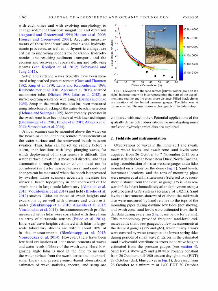
mounted on a tower on the dune (Fig. 1). Sand levels,

instrument locations, and the tops of mounting pipes

weremeasured at all in situ sensors (referred to by cross-

shore distance from the lidar, so gauge g25 is 25m sea-

ward of the lidar) immediately after deployment using a

postprocessed GPS system (accuracy of 0.02m). Sand

levels at instruments shoreward of about the midswash

also were measured by hand relative to the tops of the

mounting pipes during daytime low tides (not shown),

and swash-zone sand levels were estimated from the li-

dar data during every run (Fig. 1; see below for details).

This methodology provided frequent sand-level esti-

mates at the shallowest gauges, but fewmeasurements at

the deepest gauges (g55 and g65), which nearly always

were covered by water (except at the lowest spring tides

during periods of small waves). Errors in the estimated

sand levels could contribute to errors in the wave heights

estimated from the pressure gauges (see section 4).

Sand levels above g25 and g30 were roughly constant

from 26 October until 0800 eastern daylight time (EDT)

28 October (dark blue curves in Fig. 1), decreased from

28 October to a minimum at 1400 EDT 30 October

FIG. 1. Elevation of the sand surface [curves, colors (scale on the

right) indicate time with blue representing the start of the experi-

ment and red the end] vs cross-shore distance. Filled black circles

are locations of the buried pressure gauges. The lidar was at

distance 5 0m. The inset shows a photograph of the lidar setup.

1946 JOURNAL OF ATMOSPHER IC AND OCEAN IC TECHNOLOGY VOLUME 32

(blue through green curves), and then increased until

0700 EDT 3 November (green through orange-red

curves), before decreasing at the end of the experi-

ment (5 November, dark red curve). Sand levels above

the offshore gauges (g35–g65) were measured more

intermittently by the lidar, but they typically increased

from the start of the experiment until 1400 EDT

29 October (blue through cyan curves), and then de-

creased until 0100 EDT 2 November (green through

yellow curves), before increasing through the end of

the experiment (5 November, orange through red

curves). Beach slope, defined as the best-fit linear trend

within the swash zone, ranged between 0.02 and 0.17

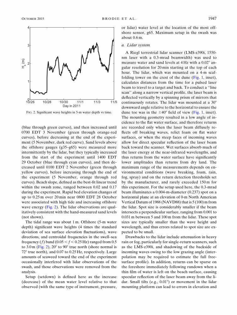
during the experiment. Rapid bed elevation changes of

up to 0.25m over 20min near 0800 EDT 28 October

were associated with high tide and increasing offshore

wave energy (Fig. 2). The lidar observations are qual-

itatively consistent with the hand-measured sand levels

(not shown).

The tidal range was about 1m. Offshore (5-m water

depth) significant wave heights (4 times the standard

deviation of sea surface elevation fluctuations), wave

directions, and centroidal frequencies in the swell–sea

frequency ( f) band (0.05, f, 0.25Hz) ranged from 0.5

to 3.0m (Fig. 2), 208 to 908 true north (shore normal is

728 true north), and 0.07 to 0.25Hz, respectively. Large

amounts of seaweed toward the end of the experiment

occasionally interfered with lidar observations of the

swash, and those observations were removed from the

analysis.

Setup (setdown) is defined here as the increase

(decrease) of the mean water level relative to that

observed (with the same type of instrument, pressure,

or lidar) water level at the location of the most off-

shore sensor, g65. Maximum setup in the swash was

about 0.6m.

a. Lidar system

A Riegl terrestrial lidar scanner (LMS-z390i, 1550-

nm laser with a 0.3-mrad beamwidth) was used to

measure water and sand levels at 4Hz with a 0.028 an-gular resolution for 20min starting at the top of each

hour. The lidar, which was mounted on a 4-m scaf-

folding tower on the crest of the dune (Fig. 1, inset),

calculates distances from the time for a pulsed laser

beam to travel to a target and back. To conduct a ‘‘line

scan’’ along a narrow vertical profile, the laser beam is

deflected vertically by a spinning prism of mirrors that

continuously rotates. The lidar was mounted at a 308downward angle relative to the horizontal to ensure the

dune toe was in the 6408 field of view (Fig. 1, inset).

The mounting geometry resulted in a low angle of in-

cidence to the flat water surface, and therefore returns

are recorded only when the laser beam diffusely re-

flects off breaking waves, relict foam on flat water

surfaces, or when the steep faces of incoming waves

allow for direct specular reflection of the laser beam

back toward the scanner. Wet surfaces absorb much of

the laser energy at the near-infrared wavelengths, and

thus returns from the water surface have significantly

lower amplitudes than returns from dry land. The

maximum range of the measurements depends on en-

vironmental conditions (wave breaking, foam, rain,

fog, spray) and on the return detection thresholds set

by the manufacturer, and rarely exceeded 150m for

this experiment. For the setup used here, the 0.3-mrad

beam illuminates a 0.004-m-diameter (0.237) spot on a

horizontal plane at an elevation of 0-m North American

Vertical Datum of 1988 (NAVD88) that is 5 (100)m from

the lidar. Spot size is considerably smaller if the beam

intersects a perpendicular surface, ranging from 0.001 to

0.031m between 5 and 100m from the lidar. These spot

sizes are typically smaller than the wave height and

wavelength, and thus errors related to spot size are ex-

pected to be small.

Drawbacks to the lidar include attenuation in heavy

rain or fog, particularly for single-return scanners, such

as the LMS-z390i, and shadowing of the backside of

incoming waves owing to the low grazing angle (inter-

polation may be required to estimate the full free-

surface profile). In addition, returns can be sparse on

the foreshore immediately following rundown when a

thin film of water is left on the beach surface, causing

specular reflection of the laser beam away from the li-

dar. Small tilts (e.g., 0.018) or movement in the lidar

mounting platform can lead to errors in elevation and

FIG. 2. Significant wave heights in 5-m water depth vs time.

OCTOBER 2015 BROD IE ET AL . 1947

position of the water and sand surfaces, especially at

long ranges. Techniques to measure and correct for

these small-scale changes in orientation of the scanner

using coregistration algorithms will be discussed in

future work, and were not applied in this study. Here,

field precision was roughly 60.015m, about twice the

manufacturer specifications, and was determined by

analyzing time series of lidar returns from the station-

ary dry beach.

To estimate foreshore slopes, run-up, and wave sta-

tistics, data were transformed from the scanner co-

ordinate system (angle and range) to rectified Cartesian

coordinates (local coordinates for the horizontal and

NAVD88 coordinates for the vertical) using a trans-

formation matrix determined from scans of GPS-

surveyed reflectors. Time differences between the first

and last data point within a single line scan are small

(0.12 s), and therefore all points within that scan were

assigned the same time. Each line scan was then inter-

polated to 0.10-m resolution in the cross-shore. To sep-

arate foreshore points from water surface points, the

line-scan elevation data were analyzed similarly to an

Argus wave run-up time stack (Holman et al. 1993), but

instead of identifying a color threshold, an elevation

threshold was used. Sand-level changes on the lower

foreshore occur on the time scale of infragravity and

swell–sea waves (Howd and Holman 1987), and thus

running minimum filters with time windows ranging

from 1.2 to 30.0 s were used to generate multiple tem-

porally varying minimum surfaces. Each minimum

surface was subtracted from the original line-scan

elevation data, and the resulting difference maps for

all minimum surfaces were averaged. For each line

scan, the most shoreward location with an elevation

. 0.015m above the average minimum surface was

identified as the run-up–beach intersection (the maxi-

mum run-up location), with seaward points classified as

water and landward points identified as the foreshore.

The run-up extraction algorithm correctly separated

water and land points only 85% of the time, because

relict foam or seaweed often interfered with the digi-

tizing, and therefore each collection was checked by

hand to ensure proper separation of water and land

points. A ‘‘mean foreshore profile’’ for each 20-min

collection was calculated by averaging the in-

stantaneous foreshore elevations (land points) at each

cross-shore location over the 20-min collection and

was used to update pressure sensor burial mea-

surements when applicable (see below).

For spectral and time series analysis, each 20-min lidar

collection was divided and segmented into two 512-s

(8.5min) sections. Mean water level is defined as the

time-averaged water level for each section of data.

Significant wave heights in the total (0.004 , f ,0.250Hz), infragravity (0.004 , f , 0.050Hz), and

swell–sea (0.050 , f , 0.250Hz) bands were estimated

from the area under the frequency spectrum.

b. In situ pressure gauges

The pressure sensors were buried (initially about

0.50–0.75m) to avoid flow-induced deviations from hy-

drostatic pressure (Raubenheimer et al. 2001). Pressure

measurements were collected at 2Hz for 51.2min,

starting at the top of each hour. Mean water levels were

calculated from the surveyed sensor location and the

time-averaged 512-s pressure measurements assuming

hydrostatic pressure and a water density of 1020kgm23.

Results were not sensitive to the chosen density value in

these shallow-water depths. Effects of temperature

changes on the pressure measurements were compen-

sated with internal temperature sensors. Pressure gauge

g35 did not start operating until 1 November.

TheGPS-measured vertical locations of g35, g45, and

g55 were adjusted (by less than 0.05m) to ensure that

the mean sea level was ‘‘flat’’ with respect to g65 over

the 512-s runs starting 1934 EDT 26 October, 0800

EDT 27 October, and 2025 EDT 27 October, when tide

levels were high and offshore wave heights (in 5-m

water depth) were less than 0.35m. Comparisons of

hand-measured sand level above the buried pressure

gauges with ‘‘sand level’’ estimated from the observa-

tions between swashes assuming hydrostatic pressure

and saturated sand agreed within the measurement

error of ;0.02m for these techniques (Raubenheimer

et al. 2001).

Sea surface fluctuations were estimated from the

pressuremeasurements using linear wave and poroelastic

theories to account for the attenuation of pressure fluc-

tuations through the water and the saturated sand above

the buried sensors, respectively [Raubenheimer et al.

1998, Eq. (5)]. Similar to the lidar observations, signifi-

cant wave heights in the total, infragravity, and swell–sea

bands were estimated from the frequency spectrum.

Water and burial depths were estimated from the sand

levels determined by the lidar and by handmeasurements

at in situ gauges in the swash at low tide.

3. Lidar–pressure comparisons

For comparison with the in situ measurements, the

lidar time series were decimated to 2Hz prior to

frequency-domain filtering and prior to estimating water

levels or wave heights. Only the two 512-s sections of

in situ data that were collected at the top of each hour

are included in the comparisons. If the beach is not

saturated, then a pressure gauge will measure the

1948 JOURNAL OF ATMOSPHER IC AND OCEAN IC TECHNOLOGY VOLUME 32

groundwater pressure head, rather than the height of the

swash or wave above the beach. Therefore, comparisons

were conducted only for locations offshore of the mean

swash (see section 4). For comparing water levels, setup,

and wave heights, the lidar and the pressure-gauge data

were time synced using cross correlation to correct for

clock drift, and squared correlation (r2), root-mean-square

error (rmse), mean bias, and best-fit linear slope statistics

were calculated on overlapping portions of the time series

(Table 1).

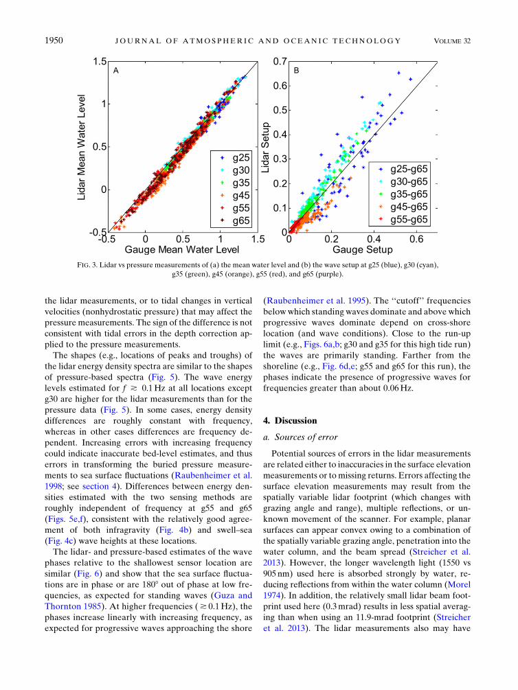
Mean water levels (relative to NAVD88) measured

with the lidar and with the pressure gauge (Fig. 3a) are

well correlated (r2 5 0.98; Table 1). The mean water

level estimated with the lidar is slightly lower (bias

of 20.07m; Table 1) than that estimated with the pres-

sure gauges, especially for the most offshore locations

and lowest water levels, possibly owing to a small tilt

in the lidar tower over the course of the experiment

that was not accounted for in the processing. Alter-

natively, the pressure measurements may be over-

estimating the mean water level owing to slight errors

in the measured vertical location of the instruments or

the process for adjusting those locations to provide a

flat sea surface (see section 2b). Although laboratory

comparisons of lidar with in situ sensors have suggested

that lidar may underestimate slightly the mean water

level (Vousdoukas et al. 2014), especially when looking

toward the oncoming waves (Blenkinsopp et al. 2012),

the cause of the (small) water-level differences shown

here is unclear (see section 4).

The lidar and pressure-estimated setup (Fig. 3b) are

well correlated (r2 5 0.92; Table 1). The low bias in the

setup measurements suggests the cause of the bias in

mean water level (Fig. 3a; Table 1) is specific to the instru-

ment type (e.g., either a consistent error in processing

methods for all pressure gauges, or a consistent error in

all the lidar measurements). However, the percent dif-

ferences in the setup estimates can be significant, par-

ticularly for g25, which was often in the swash zone.

For example, for a pressure-estimated setup of about

0.2 m (which is large offshore of the swash zone;

Raubenheimer et al. 2001), the corresponding lidar es-

timate can range from 0.1 to 0.3m (Fig. 3b). In addition,

the setup estimated by the lidar typically is a few centi-

meters lower (higher) than that estimated with the

pressure gauges at g45 (g30 and g35), possibly owing to

errors in the vertical locations of the pressure gauges

(and thus to the pressure-estimated setup), or to dif-

ferences in lidar reflectivity or shadowing by waves be-

tween the inner surf and swash.

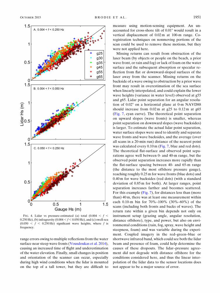
Significant wave heights (Fig. 4a) estimated with the

pressure gauges and lidar agree well (r25 0.85; Table 1).

Relative to the pressure gauge, the lidar-based wave

height estimates are slightly low at g65 and g55 and high

at g25–g45. The higher lidar estimates of wave height at

the shallower gauges may be owing to the presence of an

aerated wave roller, which would increase the elevation

of the water surface measured by the lidar, while not

affecting the pressure measured by the gauge signifi-

cantly. The lidar- and pressure-based infragravity wave

heights (Fig. 4b) are somewhat more correlated (r2 50.91; Table 1) than the total significant wave heights

(r2 5 0.85; Table 1). However, the lidar estimates are

biased high relative to the pressure estimates at g25

(Fig. 4b, blue symbols; mean difference of 0.08). In the

swell–sea band (Fig. 4c), lidar- and pressure-based es-

timates of wave height are well correlated (r2 5 0.87;

Table 1). However, the agreement is gauge dependent

(Table 1). For example, differences increase with in-

creasing wave height at g35, g45, g55, and g65 (best-fit

linear slopes . 1.0; Table 1). Lidar and pressure esti-

mates are somewhat less correlated at g25 (r2 5 0.77;

Table 1), and lidar estimates are biased high at the

shallow gauges g25, g30, and g35 (offsets of 0.10, 0.04,

and 0.09 respectively; Table 1) and low at the offshore

gauges g55 and g65 (offsets of 20.04 and 20.06 re-

spectively; Table 1). The low estimates by the lidar at the

most offshore gauges may be owing to shadowing and

drop outs in the far range of the lidar, whereas lower

correlations at g25 may be related to water table effects

within the swash zone (see section 4). Swell–sea wave

height at a fixed location increases with increasing water

depth, and thus the differences between the lidar- and

pressure-based swell–sea wave heights also fluctuate

with tidal level (not shown). The causes of these fluc-

tuations are not clear, but they could include tidal

changes in grazing angle, wave steepness, breaking wave

type or shape, foaminess, and reflectivity that may affect

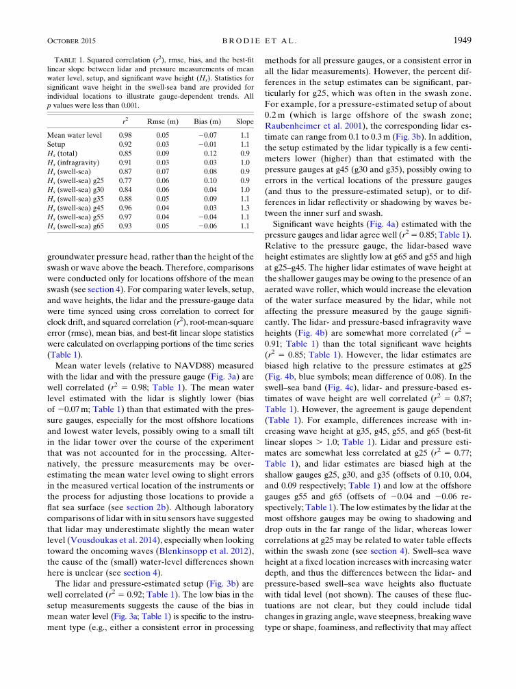
TABLE 1. Squared correlation (r2), rmse, bias, and the best-fit

linear slope between lidar and pressure measurements of mean

water level, setup, and significant wave height (Hs). Statistics for

significant wave height in the swell-sea band are provided for

individual locations to illustrate gauge-dependent trends. All

p values were less than 0.001.

r2 Rmse (m) Bias (m) Slope

Mean water level 0.98 0.05 20.07 1.1

Setup 0.92 0.03 20.01 1.1

Hs (total) 0.85 0.09 0.12 0.9

Hs (infragravity) 0.91 0.03 0.03 1.0

Hs (swell-sea) 0.87 0.07 0.08 0.9

Hs (swell-sea) g25 0.77 0.06 0.10 0.9

Hs (swell-sea) g30 0.84 0.06 0.04 1.0

Hs (swell-sea) g35 0.88 0.05 0.09 1.1

Hs (swell-sea) g45 0.96 0.04 0.03 1.3

Hs (swell-sea) g55 0.97 0.04 20.04 1.1

Hs (swell-sea) g65 0.93 0.05 20.06 1.1

OCTOBER 2015 BROD IE ET AL . 1949

the lidar measurements, or to tidal changes in vertical

velocities (nonhydrostatic pressure) that may affect the

pressure measurements. The sign of the difference is not

consistent with tidal errors in the depth correction ap-

plied to the pressure measurements.

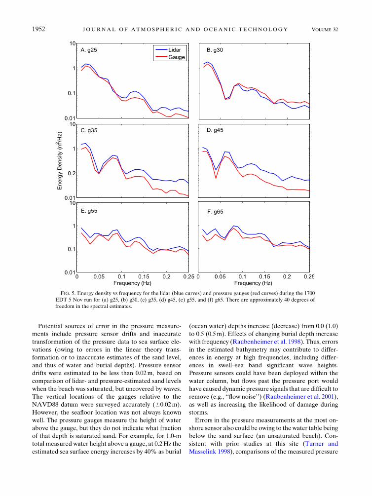
The shapes (e.g., locations of peaks and troughs) of

the lidar energy density spectra are similar to the shapes

of pressure-based spectra (Fig. 5). The wave energy

levels estimated for f * 0.1Hz at all locations except

g30 are higher for the lidar measurements than for the

pressure data (Fig. 5). In some cases, energy density

differences are roughly constant with frequency,

whereas in other cases differences are frequency de-

pendent. Increasing errors with increasing frequency

could indicate inaccurate bed-level estimates, and thus

errors in transforming the buried pressure measure-

ments to sea surface fluctuations (Raubenheimer et al.

1998; see section 4). Differences between energy den-

sities estimated with the two sensing methods are

roughly independent of frequency at g55 and g65

(Figs. 5e,f), consistent with the relatively good agree-

ment of both infragravity (Fig. 4b) and swell–sea

(Fig. 4c) wave heights at these locations.

The lidar- and pressure-based estimates of the wave

phases relative to the shallowest sensor location are

similar (Fig. 6) and show that the sea surface fluctua-

tions are in phase or are 1808 out of phase at low fre-

quencies, as expected for standing waves (Guza and

Thornton 1985). At higher frequencies (* 0.1Hz), the

phases increase linearly with increasing frequency, as

expected for progressive waves approaching the shore

(Raubenheimer et al. 1995). The ‘‘cutoff’’ frequencies

below which standing waves dominate and above which

progressive waves dominate depend on cross-shore

location (and wave conditions). Close to the run-up

limit (e.g., Figs. 6a,b; g30 and g35 for this high tide run)

the waves are primarily standing. Farther from the

shoreline (e.g., Fig. 6d,e; g55 and g65 for this run), the

phases indicate the presence of progressive waves for

frequencies greater than about 0.06Hz.

4. Discussion

a. Sources of error

Potential sources of errors in the lidar measurements

are related either to inaccuracies in the surface elevation

measurements or to missing returns. Errors affecting the

surface elevation measurements may result from the

spatially variable lidar footprint (which changes with

grazing angle and range), multiple reflections, or un-

known movement of the scanner. For example, planar

surfaces can appear convex owing to a combination of

the spatially variable grazing angle, penetration into the

water column, and the beam spread (Streicher et al.

2013). However, the longer wavelength light (1550 vs

905 nm) used here is absorbed strongly by water, re-

ducing reflections from within the water column (Morel

1974). In addition, the relatively small lidar beam foot-

print used here (0.3mrad) results in less spatial averag-

ing than when using an 11.9-mrad footprint (Streicher

et al. 2013). The lidar measurements also may have

FIG. 3. Lidar vs pressure measurements of (a) the mean water level and (b) the wave setup at g25 (blue), g30 (cyan),

g35 (green), g45 (orange), g55 (red), and g65 (purple).

1950 JOURNAL OF ATMOSPHER IC AND OCEAN IC TECHNOLOGY VOLUME 32

range errors owing tomultiple reflections from the water

surface near steep wave fronts (Vousdoukas et al. 2014),

causing an increased time of flight and underestimation

of the water elevation. Finally, small changes in position

and orientation of the scanner can occur, especially

during high wind conditions when the lidar is mounted

on the top of a tall tower, but they are difficult to

measure using motion-sensing equipment. An un-

accounted for cross-shore tilt of 0.018 would result in a

vertical displacement of 0.02m at 100-m range. Co-

registration techniques on nonmoving portions of the

scan could be used to remove these motions, but they

were not applied here.

Missing returns can result from obstruction of the

laser beam (by objects or people on the beach, a prior

wave front, or rain and fog) or lack of foam on the water

surface and the subsequent absorption or specular re-

flection from flat or downward-sloped surfaces of the

laser away from the scanner. Missing returns on the

backside of a wave owing to obstruction by a prior wave

front may result in overestimation of the sea surface

when linearly interpolated, and could explain the lower

wave heights (variance in water level) observed at g55

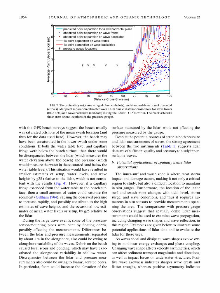
and g65. Lidar point separation for an angular resolu-

tion of 0.028 on a horizontal plane at 0-m NAVD88

should increase from 0.02m at g25 to 0.12m at g65

(Fig. 7, cyan curve). The theoretical point separation

on upward slopes (wave fronts) is smaller, whereas

point separation on downward slopes (wave backsides)

is larger. To estimate the actual lidar point separation,

water surface slopes were used to identify and separate

wave fronts and wave backsides, and the average (over

all scans in a 20-min run) distance of the nearest point

was calculated every 0.10m (Fig. 7, blue and red dots).

The theoretical flat-surface and observed point sepa-

rations agree well between 0- and 40-m range, but the

observed point separation increases more rapidly than

the flat-surface spacing between 40- and 65-m range

(the distance to the most offshore pressure gauge),

reaching roughly 0.25m for wave fronts (blue dots) and

0.40m for wave backsides (red dots) (with a standard

deviation of 0.85m for both). At larger ranges, point

separation increases farther and becomes scattered.

For this example (Fig. 7), for distances less than (more

than) 40m, there was at least one measurement within

each 0.10-m bin for 70%–100% (30%–60%) of the

scans (including both fronts and backs of waves). The

return rate within a given bin depends not only on

instrument setup (grazing angle, angular resolution,

distance offshore), type, and power, but also on envi-

ronmental conditions (rain, fog, spray, wave height and

steepness, foam) and was variable during the experi-

ment. Coupled imagery in the red–green–blue or

shortwave infrared band, which could see both the lidar

beam and presence of foam, could help determine the

causes of these dropouts. The lidar–pressure agree-

ment did not degrade with distance offshore for the

conditions considered here, and thus the linear inter-

polation of the lidar data to the sensor locations does

not appear to be a major source of error.

FIG. 4. Lidar vs pressure-estimated (a) total (0.004 , f ,0.250Hz), (b) infragravity (0.004, f, 0.050Hz), and (c) swell-sea

(0.050 , f , 0.250Hz) significant wave heights, where f is

frequency.

OCTOBER 2015 BROD IE ET AL . 1951

Potential sources of error in the pressure measure-

ments include pressure sensor drifts and inaccurate

transformation of the pressure data to sea surface ele-

vations (owing to errors in the linear theory trans-

formation or to inaccurate estimates of the sand level,

and thus of water and burial depths). Pressure sensor

drifts were estimated to be less than 0.02m, based on

comparison of lidar- and pressure-estimated sand levels

when the beach was saturated, but uncovered by waves.

The vertical locations of the gauges relative to the

NAVD88 datum were surveyed accurately (60.02m).

However, the seafloor location was not always known

well. The pressure gauges measure the height of water

above the gauge, but they do not indicate what fraction

of that depth is saturated sand. For example, for 1.0-m

total measured water height above a gauge, at 0.2Hz the

estimated sea surface energy increases by 40% as burial

(ocean water) depths increase (decrease) from 0.0 (1.0)

to 0.5 (0.5m). Effects of changing burial depth increase

with frequency (Raubenheimer et al. 1998). Thus, errors

in the estimated bathymetry may contribute to differ-

ences in energy at high frequencies, including differ-

ences in swell–sea band significant wave heights.

Pressure sensors could have been deployed within the

water column, but flows past the pressure port would

have caused dynamic pressure signals that are difficult to

remove (e.g., ‘‘flow noise’’) (Raubenheimer et al. 2001),

as well as increasing the likelihood of damage during

storms.

Errors in the pressure measurements at the most on-

shore sensor also could be owing to the water table being

below the sand surface (an unsaturated beach). Con-

sistent with prior studies at this site (Turner and

Masselink 1998), comparisons of the measured pressure

FIG. 5. Energy density vs frequency for the lidar (blue curves) and pressure gauges (red curves) during the 1700

EDT 5 Nov run for (a) g25, (b) g30, (c) g35, (d) g45, (e) g55, and (f) g65. There are approximately 40 degrees of

freedom in the spectral estimates.

1952 JOURNAL OF ATMOSPHER IC AND OCEAN IC TECHNOLOGY VOLUME 32

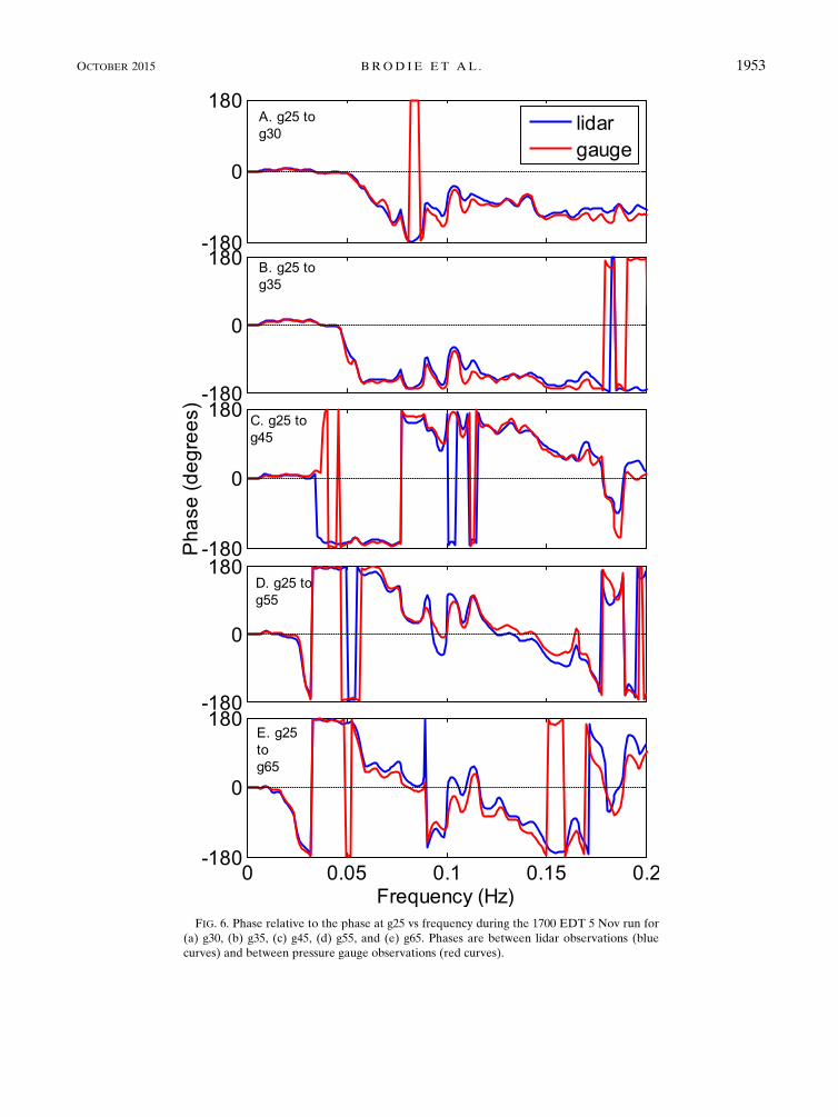
FIG. 6. Phase relative to the phase at g25 vs frequency during the 1700 EDT 5 Nov run for

(a) g30, (b) g35, (c) g45, (d) g55, and (e) g65. Phases are between lidar observations (blue

curves) and between pressure gauge observations (red curves).

OCTOBER 2015 BROD IE ET AL . 1953

with the GPS beach surveys suggest the beach usually

was saturated offshore of the mean swash location (and

thus for the data used here). However, the beach may

have been unsaturated in the lower swash under some

conditions. If both the water table level and capillary

fringe were below the beach surface, then there would

be discrepancies between the lidar (which measures the

water elevation above the beach) and pressure (which

wouldmeasure the water in the saturated sand below the

water table level). This situation would have resulted in

smaller estimates of setup, water levels, and wave

heights by g25 relative to the lidar, which is not consis-

tent with the results (Fig. 4). However, if a capillary

fringe extended from the water table to the beach sur-

face, then a small amount of water could saturate the

sediment (Gillham 1984), causing the observed pressure

to increase rapidly, and possibly contribute to the high

estimates of wave heights, and the occasional low esti-

mates of mean water levels or setup, by g25 relative to

the lidar.

During the large wave events, some of the pressure-

sensor-mounting pipes were bent by floating debris,

possibly affecting the measurements. Differences be-

tween the lidar and pressure measurements, separated

by about 1m in the alongshore, also could be owing to

alongshore variability of the waves. Debris on the beach

caused local scour and ponding, which may have exac-

erbated the alongshore variability in shallow water.

Discrepancies between the lidar and pressure mea-

surements also could be owing to foamy, aerated bores.

In particular, foam could increase the elevation of the

surface measured by the lidar, while not affecting the

pressure measured by the gauge.

Despite the potential sources of error in both pressure

and lidar measurements of waves, the strong agreement

between the two instruments (Table 1) suggests lidar

data are of sufficient quality and accuracy to study inner-

surfzone waves.

b. Potential applications of spatially dense lidarobservations

The inner-surf and swash zone is where most storm

impact and damage occurs, making it not only a critical

region to study, but also a difficult location to maintain

in situ gauges. Furthermore, the location of the inner

surf and swash zone changes with tidal level, storm

surge, and wave conditions, and thus it requires nu-

merous in situ sensors to provide measurements span-

ning the area. The comparisons with pressure-gauge

observations suggest that spatially dense lidar mea-

surements could be used to examine wave propagation,

including changing wave shapes and wave reflection, in

this region. Examples are given below to illustrate some

potential applications of lidar data and to evaluate the

lidar for these uses.

As waves shoal and dissipate, wave shapes evolve ow-

ing to nonlinear energy exchanges and phase coupling.

Changing wave shape affects velocity asymmetries, which

can affect sediment transport magnitudes and directions,

as well as impact forces on underwater structures. Posi-

tive wave skewness indicates sharper wave crests and

flatter troughs, whereas positive asymmetry indicates

FIG. 7. Theoretical (cyan), run-averaged observed (dots), and standard deviation of observed

(curves) lidar point separation estimated over 0.1-m bins vs distance cross-shore for wave fronts

(blue dots) and wave backsides (red dots) during the 1700 EDT 5 Nov run. The black asterisks

show cross-shore locations of the pressure gauges.

1954 JOURNAL OF ATMOSPHER IC AND OCEAN IC TECHNOLOGY VOLUME 32

steep front faces and more gently sloped rear faces

(Masuda and Kuo 1981; Elgar and Guza 1985a; Doering

and Bowen 1995). The cross-shore trends in pressure-

and lidar-based skewness and asymmetry qualitatively

are consistent with each other, and with earlier results.

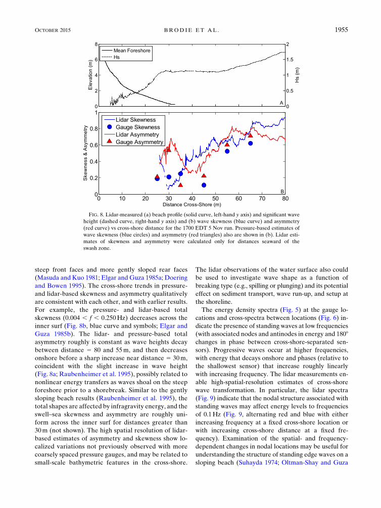
For example, the pressure- and lidar-based total

skewness (0.004 , f , 0.250Hz) decreases across the

inner surf (Fig. 8b, blue curve and symbols; Elgar and

Guza 1985b). The lidar- and pressure-based total

asymmetry roughly is constant as wave heights decay

between distance 5 80 and 55m, and then decreases

onshore before a sharp increase near distance 5 30m,

coincident with the slight increase in wave height

(Fig. 8a; Raubenheimer et al. 1995), possibly related to

nonlinear energy transfers as waves shoal on the steep

foreshore prior to a shorebreak. Similar to the gently

sloping beach results (Raubenheimer et al. 1995), the

total shapes are affected by infragravity energy, and the

swell–sea skewness and asymmetry are roughly uni-

form across the inner surf for distances greater than

30m (not shown). The high spatial resolution of lidar-

based estimates of asymmetry and skewness show lo-

calized variations not previously observed with more

coarsely spaced pressure gauges, and may be related to

small-scale bathymetric features in the cross-shore.

The lidar observations of the water surface also could

be used to investigate wave shape as a function of

breaking type (e.g., spilling or plunging) and its potential

effect on sediment transport, wave run-up, and setup at

the shoreline.

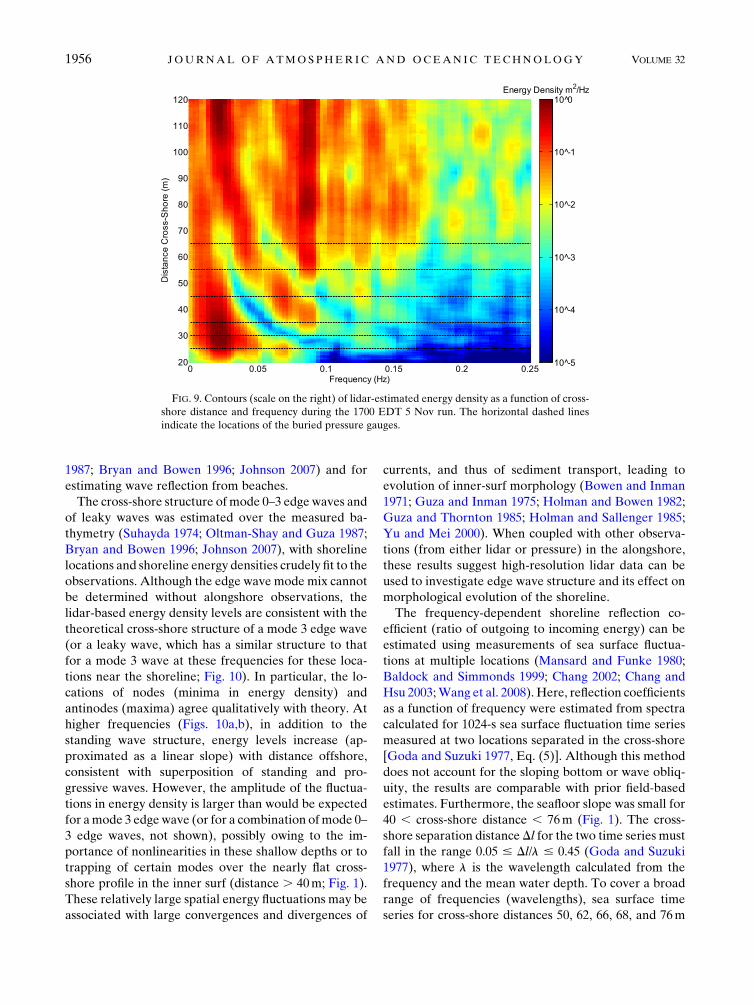
The energy density spectra (Fig. 5) at the gauge lo-

cations and cross-spectra between locations (Fig. 6) in-

dicate the presence of standing waves at low frequencies

(with associated nodes and antinodes in energy and 1808changes in phase between cross-shore-separated sen-

sors). Progressive waves occur at higher frequencies,

with energy that decays onshore and phases (relative to

the shallowest sensor) that increase roughly linearly

with increasing frequency. The lidar measurements en-

able high-spatial-resolution estimates of cross-shore

wave transformation. In particular, the lidar spectra

(Fig. 9) indicate that the nodal structure associated with

standing waves may affect energy levels to frequencies

of 0.1Hz (Fig. 9, alternating red and blue with either

increasing frequency at a fixed cross-shore location or

with increasing cross-shore distance at a fixed fre-

quency). Examination of the spatial- and frequency-

dependent changes in nodal locations may be useful for

understanding the structure of standing edge waves on a

sloping beach (Suhayda 1974; Oltman-Shay and Guza

FIG. 8. Lidar-measured (a) beach profile (solid curve, left-hand y axis) and significant wave

height (dashed curve, right-hand y axis) and (b) wave skewness (blue curve) and asymmetry

(red curve) vs cross-shore distance for the 1700 EDT 5 Nov run. Pressure-based estimates of

wave skewness (blue circles) and asymmetry (red triangles) also are shown in (b). Lidar esti-

mates of skewness and asymmetry were calculated only for distances seaward of the

swash zone.

OCTOBER 2015 BROD IE ET AL . 1955

1987; Bryan and Bowen 1996; Johnson 2007) and for

estimating wave reflection from beaches.

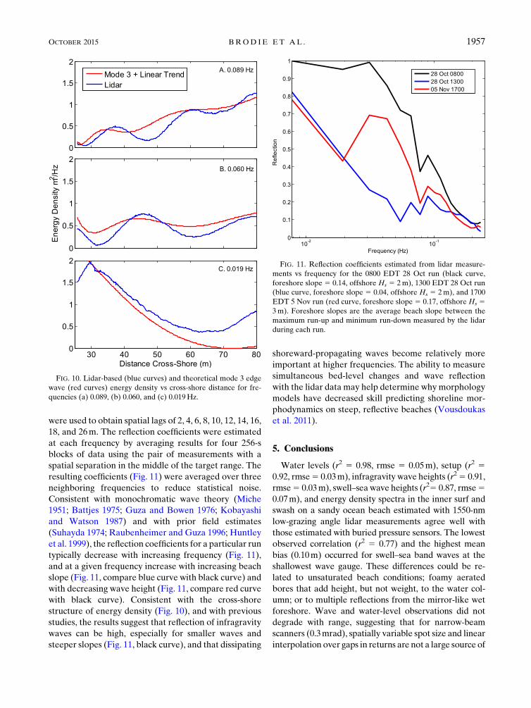
The cross-shore structure ofmode 0–3 edge waves and

of leaky waves was estimated over the measured ba-

thymetry (Suhayda 1974; Oltman-Shay and Guza 1987;

Bryan and Bowen 1996; Johnson 2007), with shoreline

locations and shoreline energy densities crudely fit to the

observations. Although the edge wave mode mix cannot

be determined without alongshore observations, the

lidar-based energy density levels are consistent with the

theoretical cross-shore structure of a mode 3 edge wave

(or a leaky wave, which has a similar structure to that

for a mode 3 wave at these frequencies for these loca-

tions near the shoreline; Fig. 10). In particular, the lo-

cations of nodes (minima in energy density) and

antinodes (maxima) agree qualitatively with theory. At

higher frequencies (Figs. 10a,b), in addition to the

standing wave structure, energy levels increase (ap-

proximated as a linear slope) with distance offshore,

consistent with superposition of standing and pro-

gressive waves. However, the amplitude of the fluctua-

tions in energy density is larger than would be expected

for amode 3 edgewave (or for a combination ofmode 0–

3 edge waves, not shown), possibly owing to the im-

portance of nonlinearities in these shallow depths or to

trapping of certain modes over the nearly flat cross-

shore profile in the inner surf (distance . 40m; Fig. 1).

These relatively large spatial energy fluctuations may be

associated with large convergences and divergences of

currents, and thus of sediment transport, leading to

evolution of inner-surf morphology (Bowen and Inman

1971; Guza and Inman 1975; Holman and Bowen 1982;

Guza and Thornton 1985; Holman and Sallenger 1985;

Yu and Mei 2000). When coupled with other observa-

tions (from either lidar or pressure) in the alongshore,

these results suggest high-resolution lidar data can be

used to investigate edge wave structure and its effect on

morphological evolution of the shoreline.

The frequency-dependent shoreline reflection co-

efficient (ratio of outgoing to incoming energy) can be

estimated using measurements of sea surface fluctua-

tions at multiple locations (Mansard and Funke 1980;

Baldock and Simmonds 1999; Chang 2002; Chang and

Hsu 2003;Wang et al. 2008). Here, reflection coefficients

as a function of frequency were estimated from spectra

calculated for 1024-s sea surface fluctuation time series

measured at two locations separated in the cross-shore

[Goda and Suzuki 1977, Eq. (5)]. Although this method

does not account for the sloping bottom or wave obliq-

uity, the results are comparable with prior field-based

estimates. Furthermore, the seafloor slope was small for

40 , cross-shore distance , 76m (Fig. 1). The cross-

shore separation distance Dl for the two time series must

fall in the range 0.05 # Dl/l # 0.45 (Goda and Suzuki

1977), where l is the wavelength calculated from the

frequency and the mean water depth. To cover a broad

range of frequencies (wavelengths), sea surface time

series for cross-shore distances 50, 62, 66, 68, and 76m

FIG. 9. Contours (scale on the right) of lidar-estimated energy density as a function of cross-

shore distance and frequency during the 1700 EDT 5 Nov run. The horizontal dashed lines

indicate the locations of the buried pressure gauges.

1956 JOURNAL OF ATMOSPHER IC AND OCEAN IC TECHNOLOGY VOLUME 32

were used to obtain spatial lags of 2, 4, 6, 8, 10, 12, 14, 16,

18, and 26m. The reflection coefficients were estimated

at each frequency by averaging results for four 256-s

blocks of data using the pair of measurements with a

spatial separation in the middle of the target range. The

resulting coefficients (Fig. 11) were averaged over three

neighboring frequencies to reduce statistical noise.

Consistent with monochromatic wave theory (Miche

1951; Battjes 1975; Guza and Bowen 1976; Kobayashi

and Watson 1987) and with prior field estimates

(Suhayda 1974; Raubenheimer and Guza 1996; Huntley

et al. 1999), the reflection coefficients for a particular run

typically decrease with increasing frequency (Fig. 11),

and at a given frequency increase with increasing beach

slope (Fig. 11, compare blue curve with black curve) and

with decreasing wave height (Fig. 11, compare red curve

with black curve). Consistent with the cross-shore

structure of energy density (Fig. 10), and with previous

studies, the results suggest that reflection of infragravity

waves can be high, especially for smaller waves and

steeper slopes (Fig. 11, black curve), and that dissipating

shoreward-propagating waves become relatively more

important at higher frequencies. The ability to measure

simultaneous bed-level changes and wave reflection

with the lidar data may help determine why morphology

models have decreased skill predicting shoreline mor-

phodynamics on steep, reflective beaches (Vousdoukas

et al. 2011).

5. Conclusions

Water levels (r2 5 0.98, rmse 5 0.05m), setup (r2 50.92, rmse5 0.03m), infragravity wave heights (r25 0.91,

rmse5 0.03m), swell–sea wave heights (r25 0.87, rmse50.07m), and energy density spectra in the inner surf and

swash on a sandy ocean beach estimated with 1550-nm

low-grazing angle lidar measurements agree well with

those estimated with buried pressure sensors. The lowest

observed correlation (r2 5 0.77) and the highest mean

bias (0.10m) occurred for swell–sea band waves at the

shallowest wave gauge. These differences could be re-

lated to unsaturated beach conditions; foamy aerated

bores that add height, but not weight, to the water col-

umn; or to multiple reflections from the mirror-like wet

foreshore. Wave and water-level observations did not

degrade with range, suggesting that for narrow-beam

scanners (0.3mrad), spatially variable spot size and linear

interpolation over gaps in returns are not a large source of

FIG. 10. Lidar-based (blue curves) and theoretical mode 3 edge

wave (red curves) energy density vs cross-shore distance for fre-

quencies (a) 0.089, (b) 0.060, and (c) 0.019Hz.

FIG. 11. Reflection coefficients estimated from lidar measure-

ments vs frequency for the 0800 EDT 28 Oct run (black curve,

foreshore slope 5 0.14, offshore Hs 5 2m), 1300 EDT 28 Oct run

(blue curve, foreshore slope 5 0.04, offshore Hs 5 2m), and 1700

EDT 5 Nov run (red curve, foreshore slope 5 0.17, offshore Hs 53m). Foreshore slopes are the average beach slope between the

maximum run-up and minimum run-down measured by the lidar

during each run.

OCTOBER 2015 BROD IE ET AL . 1957

error for these conditions. The maximum range of the

lidar observations and percentage of pulses returned

were dependent on environmental conditions (foam,

wave heights, rain, fog, spray), with the maximum range

for this scanner over this time period reaching 150m. The

lidar and pressure observations indicate that standing

infragravity waves dominate the energy at low frequen-

cies and progressive swell–sea waves dominate at higher

frequencies, consistent with prior studies. Reflection co-

efficients, estimated from lidar measurements at pairs of

locations with different spatial lags to cover a wide range

of frequencies (or wavelengths), are high at low fre-

quencies, increase with beach slope, and decrease with

increasing offshore wave height. Lidar data suggest that

wave asymmetry increases rapidly just offshore of the

swash. Drawbacks to the lidar include degraded perfor-

mance during heavy rain and the potential for rectifica-

tion errors at far range from uncorrected sensor

movement. The comparisons with pressure measure-

ments presented here, prior studies, and theory demon-

strate that lidar measures inner-surf waves and setup

accurately, and can be a useful tool for investigating

inner-surf and swash zone hydrodynamics.

Acknowledgments. We thank Brian Scarborough,

Jason Pipes, and Mark Preisser for erecting the lidar

scaffolding, for operating the jetting equipment used to

deploy and recover the instruments, and for clearing huge

piles of sea grass off the beach; Dan Freer for electronics

support; Seth Zippel for programming the pressure

gauges and for retrieving the data; and Danik Forsman,

Melissa Moulton, Jenna Walker, and Regina Yopak for

assisting throughout the field study. Funding was provided

by the USACE Coastal Field Data Collection (CFDC)

and Coastal Ocean Data Systems (CODS) programs, the

Office of Naval Research, the National Science Founda-

tion, and the Assistant Secretary of Defense (R&E).

REFERENCES

Aagaard, T., and B. Greenwood, 1994: Suspended sediment trans-

port and the role of infragravity waves in a barred surf zone.

Mar. Geol., 118, 23–48, doi:10.1016/0025-3227(94)90111-2.

Almeida, L. P., G. Masselink, P. E. Russell, M. Davidson, T. Poate,

R.Mccall, C. Blenkinsopp, and I. L. Turner, 2013:Observations

of the swash zone on a gravel beach during a stormusing a laser-

scanner (Lidar). J. Coastal Res., 65, 636–641, doi:10.2112/

SI65-108.1.

Apotsos, A., B. Raubenheimer, S. Elgar, and R. T. Guza, 2008:

Wave-driven setup and alongshore flows observed onshore of a

submarine canyon. J. Geophys. Res., 113, C07025, doi:10.1029/

2007JC004514.

Baldock, T.E., andD. J. Simmonds, 1999: Separation of incident and

reflected waves over sloping bathymetry.Coastal Eng., 38, 167–

176, doi:10.1016/S0378-3839(99)00046-0.

Battjes, J. A., 1975: Surf similarity. Proceedings of the 14th Con-

ference on Coastal Engineering, Vol. 1, ASCE, 466–480.

——, and M. J. F. Stive, 1985: Calibration and verification of a

dissipation model for random breaking waves. J. Geophys.

Res., 90, 9159–9167, doi:10.1029/JC090iC05p09159.

Beach, R. A., and R. W. Sternberg, 1988: Suspended sediment trans-

port in the surf zone:Response to cross-shore infragravitymotion.

Mar. Geol., 80, 61–79, doi:10.1016/0025-3227(88)90072-2.

Blenkinsopp, C. E.,M.A.Mole, I. L. Turner, andW. L. Peirson, 2010:

Measurements of the time-varying free-surface profile across the

swash zone obtained using an industrial LIDAR. Coastal Eng.,

57, 1059–1065, doi:10.1016/j.coastaleng.2010.07.001.——, I. L. Turner, M. J. Allis, W. L. Peirson, and L. E. Garden,

2012: Application of LiDAR technology for measurement of

time-varying free-surface profiles in a laboratory wave flume.

Coastal Eng., 68, 1–5, doi:10.1016/j.coastaleng.2012.04.006.

Bowen,A. J., andD. L. Inman, 1971: Edgewaves and crescentic bars.

J. Geophys. Res., 76, 8662–8671, doi:10.1029/JC076i036p08662.Brodie, K. L., R. K. Slocum, and J. E. McNinch, 2012: New insights

into the physical drivers of wave runup from a continuously

operating terrestrial laser scanner. 2012 Oceans, IEEE, 8 pp.,

doi:10.1109/OCEANS.2012.6404955.

Bryan, K. R., and A. J. Bowen, 1996: Edge wave trapping and

amplification on barred beaches. J. Geophys. Res., 101, 6543–

6552, doi:10.1029/95JC03627.

Chang, H. K., 2002: A three-point method for separating incident and

reflectedwaves over a sloping bed.ChinaOceanEng., 16, 499–512.

——, and T. W. Hsu, 2003: A two-point method for estimating

wave reflection over a sloping beach. Ocean Eng., 30, 1833–

1847, doi:10.1016/S0029-8018(03)00017-9.

Doering, J. C., and A. J. Bowen, 1995: Parameterization of orbital ve-

locity asymmetries of shoaling and breaking waves using bispectral

analysis.CoastalEng.,26, 15–33, doi:10.1016/0378-3839(95)00007-X.

Elgar, S., andR. T.Guza, 1985a:Observations of bispectra of shoaling

surface gravity waves. J. Fluid Mech., 161, 425–448, doi:10.1017/

S0022112085003007.

——, and ——, 1985b: Shoaling gravity waves: Comparisons be-

tween field observations, linear theory, and a nonlinearmodel.

J. Fluid Mech., 158, 47–70, doi:10.1017/S0022112085002543.

Gillham, R. W., 1984: The capillary fringe and its effect on water-table

response. J. Hydrol., 67, 307–324, doi:10.1016/0022-1694(84)90248-8.Goda, Y., and Y. Suzuki, 1977: Estimation of incident and reflected

waves in random wave experiments. Proceedings of the 15th

Coastal Engineering Conference, Vol. 1, ASCE, 828–845.

Guza, R. T., and D. L. Inman, 1975: Edge waves and beach cusps.

J. Geophys. Res., 80, 2997–3012, doi:10.1029/JC080i021p02997.

——, and A. J. Bowen, 1976: Resonant interactions for waves

breaking on a beach. Proceedings of the 15th Conference on

Coastal Engineering, Vol. 1, ASCE, 560–579.

——, andE. B. Thornton, 1982: Swash oscillations on a natural beach.

J. Geophys. Res., 87, 483–491, doi:10.1029/JC087iC01p00483.

——, and ——, 1985: Observations of surf beat. J. Geophys. Res.,

90, 3161–3172, doi:10.1029/JC090iC02p03161.Haas, K. A., I. A. Svendsen, M. C. Haller, and Q. Zhao, 2003:

Quasi-three dimensional modeling of rip current systems.

J. Geophys. Res., 108, 3217, doi:10.1029/2002JC001355.

Haller, M. C., R. A. Dalrymple, and I. A. Svendsen, 2002: Experi-

mental study of nearshore dynamics on a barred beach with rip

channels. J. Geophys. Res., 107, 3061, doi:10.1029/2001JC000955.Hansen, J., T. T. Janssen, B. Raubenheimer, F. Shi, P. Barnard, and

I. Jones, 2014: Observations of surfzone alongshore pressure

gradients onshore of an ebb-tidal delta. Coastal Eng., 91, 251–

260, doi:10.1016/j.coastaleng.2014.05.010.

1958 JOURNAL OF ATMOSPHER IC AND OCEAN IC TECHNOLOGY VOLUME 32

Holman, R. A., and A. J. Bowen, 1982: Bars, bumps and holes:

Models for the generation of complex beach topography.

J. Geophys. Res., 87, 457–468, doi:10.1029/JC087iC01p00457.

——, andA.H. Sallenger, 1985: Setup and swash on a natural beach.

J. Geophys. Res., 90, 945–953, doi:10.1029/JC090iC01p00945.

Holman, R., A. Sallenger, T. Lippmann, and J. Haines, 1993: The

application of video image processing to the study of nearshore

processes.Oceanography, 6, 78–85, doi:10.5670/oceanog.1993.02.Houser, C., and B. Greenwood, 2007: Onshore migration of a

swash bar during a storm. J. Coastal Res., 23, 1–14, doi:10.2112/

03-0135.1.

——, ——, and T. Aagaard, 2006: Divergent response of an inter-

tidal swash bar. Earth Surf. Processes Landforms, 31, 1775–

1791, doi:10.1002/esp.1365.

Howd, P. A., and R. A. Holman, 1987: A simple model of beach

foreshore response to long-period waves. Mar. Geol., 78, 11–

22, doi:10.1016/0025-3227(87)90065-X.

Huntley, D. A., D. Simmonds, and R. Tatavarti, 1999: Use of

collocated sensors to measure coastal wave reflection.

J. Waterw. Port Coastal Ocean Eng., 125, 46–52, doi:10.1061/

(ASCE)0733-950X(1999)125:1(46).

Jafari, A., N. Cartwright, and P. Nielsen, 2012: Manometer tubes for

monitoring coastal water levels: New frequency response factors.

Coastal Eng., 66, 35–39, doi:10.1016/j.coastaleng.2012.03.010.

Johnson, R. S., 2007: Edge waves: theories past and present.Philos.

Trans. Roy. Soc. London, 365A, doi:10.1098/rsta.2007.2013.

King, B. A., M. W. L. Blackley, A. P. Carr, and P. J. Hardcastle, 1990:

Observations of wave-induced setup on a natural beach.

J.Geophys.Res., 95, 22 289–22 297, doi:10.1029/JC095iC12p22289.

Kobayashi, N., and K. D.Watson, 1987:Wave reflection and runup

on smooth slopes. Coastal Hydrodynamics: Proceedings of a

Conference Sponsored by the Waterway, Port, Coastal and

Ocean Division of the American Society of Civil Engineers,

R. A. Dalrymple, Ed., ASCE, 548–563.

——, and H. Jung, 2012: Beach erosion and recovery. J. Waterw.

Port Coastal Ocean Eng., 138, 473–483, doi:10.1061/

(ASCE)WW.1943-5460.0000147.

Lentz, S., and B. Raubenheimer, 1999: Field observations of wave

setup. J. Geophys. Res., 104, 25 867–25 875, doi:10.1029/

1999JC900239.

Mansard, E. P. D., and E. R. Funke, 1980: The measurement of

incident and reflected spectra using a least squares method.

17th International Conference on Coastal Engineering, B. L.

Edge, Ed., ASCE, 154–172.

Masselink,G., andS. vanHeteren, 2014:Responseofwave-dominated

and mixed-energy barriers to storms. Mar. Geol., 352, 321–347,

doi:10.1016/j.margeo.2013.11.004.

Masuda, A., and Y.-Y. Kuo, 1981: A note on the imaginary part

of bispectra. Deep-Sea Res., 28A, 213–222, doi:10.1016/

0198-0149(81)90063-7.

Miche, R., 1951: Le pouvoir réfléchissant des ouvrages maritimes

exposés à l’action de la houle.Ann.PontsChaussees, 121, 285–319.Morel, A., 1974: Optical properties of pure water and pure sea

water.Optical Aspects of Oceanography, N. G. Jerlov and E.S.

Nielson, Eds., Academic Press Inc., 1–24.

Nielsen, P., 1988:Wave setup:Afield study. J.Geophys.Res.,93, 15 643–15 652, doi:10.1029/JC093iC12p15643.

Oltman-Shay, J., and R. T. Guza, 1987: Infragravity edge wave obser-

vations on twoCaliforniabeaches. J. Phys.Oceanogr.,17, 644–663,

doi:10.1175/1520-0485(1987)017,0644:IEWOOT.2.0.CO;2.

Puleo, J. A., and Coauthors, 2014: A comprehensive field study of

swash-zone processes. I: Experimental design with examples

of hydrodynamic and sediment transport measurements.

J. Waterw. Port Coastal Ocean Eng., 140, 14–28, doi:10.1061/

(ASCE)WW.1943-5460.0000210.

Putrevu, U., J. Oltman-Shay, and I. A. Svendsen, 1995: Effect of

alongshore nonuniformities on longshore current predictions.

J. Geophys. Res., 100, 16 119–16 130, doi:10.1029/95JC01459.

Raubenheimer, B., andR. T.Guza, 1996:Observations and predictions

of run-up. J. Geophys. Res., 101, 25 575–25 587, doi:10.1029/

96JC02432.

——, ——, S. Elgar, and N. Kobayashi, 1995: Swash on a gently

sloping beach. J. Geophys. Res., 100, 8751–8760, doi:10.1029/

95JC00232.

——, S. Elgar, and R. T. Guza, 1998: Estimating wave heights from

pressuremeasured ina sandbed. J.Waterw.PortCoast.OceanEng.,

124, 151–154, doi:10.1061/(ASCE)0733-950X(1998)124:3(151).

——,R. T.Guza, and S. Elgar, 2001: Field observations of wave-driven

setdown and setup. J. Geophys. Res., 106, 4629–4638, doi:10.1029/

2000JC000572.

Sallenger, A. H., Jr., 2000: Storm impact scale for barrier islands.

J. Coastal Res., 16, 890–895.

Stockdon,H. F., A. H. Sallenger, R.A.Holman, and P.A.Howd, 2007:

A simple model for the spatially-variable coastal response to hur-

ricanes.Mar. Geol., 238, 1–20, doi:10.1016/j.margeo.2006.11.004.

Streicher, M., B. Hofland, and R. C. Linderbergh, 2013: Laser

ranging for monitoring water waves in the newDeltares Delta

Flume. ISPRS Workshop Laser Scanning 2013, M. Scaioni

et al., Eds., Vol. II-5/W2, ISPRS, 265–270.

Suhayda, J. N., 1974: Standing waves on beaches. J. Geophys. Res.,

79, 3065–3071, doi:10.1029/JC079i021p03065.Turner, I. L., andG.Masselink, 1998: Swash infiltration-exfiltration

and sediment transport. J. Geophys. Res., 103, 30 813–30 824,

doi:10.1029/98JC02606.

vanRooijen, A. Reniers, J. van Thiel deVries, C. Blenkinsopp, and

R. McCall, 2012: Modeling swash zone sediment transport at

Truc Vert Beach. 33rd Conference on Coastal Engineering

2012, P. Lynett and J. McKee Smith, Eds., Vol. 4, ICCE, 3265–

3276.

Vousdoukas,M. I., L. P. Almeida, andÓ. Ferreira, 2011:Modelling

storm-induced beach morphological change in a meso-tidal,

reflective beach using XBeach. J. Coastal Res., 64, 1960–1920.——, T. Kirupakaramoorthy, H. Oumeraci, M. de la Torre,

F. Wübbold, B. Wagner, and S. Schimmels, 2014: The role of

combined laser scanning and video techniques in monitoring

wave-by-wave swash zone processes. Coastal Eng., 83, 150–165, doi:10.1016/j.coastaleng.2013.10.013.

Wang, S.-K., T.-W. Hsu,W.-K.Weng, and S.-H. Ou, 2008: A three-

point method for estimating wave reflection of obliquely in-

cident waves over a sloping bottom.Coastal Eng., 55, 125–138,

doi:10.1016/j.coastaleng.2007.09.002.

Yu, J., and C. C. Mei, 2000: Formation of sand bars under

surface waves. J. Fluid Mech., 416, 315–348, doi:10.1017/S0022112000001063.

OCTOBER 2015 BROD IE ET AL . 1959