Embed Size (px)
Citation preview
Improved Understanding of Performance of Local Controls
Linking the above and below Ground Components of Urban
Flood Flows
Submitted by
Istvan Galambos
to the
University of Exeter
as a thesis for the degree of
Doctor of Philosophy in Engineering
July 2012
This thesis is available for Library use on the understanding that it is copyright
material and that no quotation from the thesis may be published without proper
acknowledgement.
I certify that all material in this thesis which is not my own work has been
identified and that no material has previously been submitted and approved for
the award of a degree by this or any other University.

2
...dedicated to my family, with love and gratitude...
3
Abstract
This work is devoted to investigation of the flow interaction between above and
below ground drainage systems through gullies. Nowadays frequent flood events
reinforce the need for using accurate models to simulate flooding and help urban
drainage engineers. A source of uncertainty in these models is the lack of
understanding of the complex interactions between the above and below ground
drainage systems.
The work is divided into two distinct parts. The first one focuses on the
development of the solution method. The method is based on the unstructured,
two- and three-dimensional finite volume method using the Volume of Fluid
(VOF) surface capturing technique. A novel method used to link the 3D and 2D
domains is developed in order to reduce the simulation time.
The second part concentrates on the validation and implementation of the
Computational Fluid Dynamics (CFD) model. The simulation results have been
compared against 1:1 scale experimental tests. The agreement between the
predictions and the experimental data is found to be satisfactory. The CFD
simulation of the different flow configurations for a gully provides a detailed
insight into the dynamics of the flow. The computational results provide all the
flow details which are inaccessible by present experimental techniques and they
are used to prove theoretical assumptions which are important for flood
modelling and gully design.

4
Acknowledgements
First of all I would like to express my gratitude to my supervisors, Dr Slobodan
Djordjevic and Dr Gavin Tabor for their support and guidance throughout my
research carried out at the University of Exeter during the past four years. I
appreciate their valuable guidance on the subject and the freedom that gave me
to develop my own interests.
I am deeply grateful for Prof. Adrian Saul, Naridah Sabtu and Gavin Sailor for
the provision of experimental data. I am thankful to Dr Zeljko Tukovic for
helping me clarify many tricky numerical issues. Valuable suggestions of Dr
Hrvoje Jasak are gratefully acknowledged.
The research presented in this Thesis was funded through the Flood Risk
Management Research Consortium (FRMRC) Research Priority Area X Urban
Flood Management, which was lead by Professor Adrian Saul. The Consortium
was funded by the UK Engineering and Physical Sciences Research Council
under grant GR/S76304/01, jointly with the UK Natural Environment Research
Council, the Department of Environment, Food and Rural Affairs, The
Environment Agency of England and Wales, the Scottish Executive, the Rivers
Agency (Northern Ireland) and the UK Water Industry Research.
5
Table of Contents
Contents
Chapter 1 Introduction ..................................................................................... 17
1.1 Motivation ........................................................................................ 18
1.2 Objectives ......................................................................................... 19
1.3 Structure of thesis ............................................................................ 20
Chapter 2 Previous and Related Studies ........................................................... 21
2.1 Grate Inlet ........................................................................................ 21
2.2 Discharge Coefficient ........................................................................ 27
2.3 Linking surface and sub-surface networks ........................................ 32
2.4 CFD Modelling ................................................................................. 35
2.5 Conclusion ........................................................................................ 38
Chapter 3 Description of Physical Experiments completed in the Sheffield
Laboratory........................................................................................ 41
3.1 Experimental rig ............................................................................... 41
3.1.1 Testing platform ............................................................................ 41
3.1.2 Gully and grates ............................................................................ 43
6
3.1.3 Pressure transducer and point-gauge ............................................. 45
3.2 Terminal system ............................................................................... 46
3.3 Intermediate system ......................................................................... 47
3.4 Surcharged system ............................................................................ 48
3.5 Testing protocol ............................................................................... 49
Chapter 4 CFD Modelling ................................................................................. 50
4.1 Interface capturing methods ............................................................. 52
4.2 Mathematical model ......................................................................... 58
4.2.1 Navier-Stokes equations ................................................................. 58
4.2.2 Turbulence modelling .................................................................... 60
4.2.3 Final form of equations .................................................................. 63
4.2.4 Initial and boundary conditions ..................................................... 65
4.3 Numerical Model .............................................................................. 67
4.3.1 Introduction ................................................................................... 67
4.3.2 Full 3D model ................................................................................ 68
4.3.3 Novel nested 2D/3D approach ....................................................... 82
4.4 Mesh Creation .................................................................................. 94
4.4.1 Tetrahedral mesh ........................................................................... 97
4.4.2 Hybrid mesh .................................................................................. 97
4.4.3 Mesh quality ................................................................................ 100
7
Chapter 5 Results............................................................................................ 104
5.1 CFD Model validation .................................................................... 104
5.1.1 Flow into gully ............................................................................ 105
5.1.2 Surcharged gully .......................................................................... 122
5.2 CFD model application for flow into and from gully ...................... 125
5.3 Interception capacity ...................................................................... 129
5.3.1 Factors affecting grating efficiency .............................................. 136
5.4 Surcharging conditions ................................................................... 142
5.5 Discharge coefficient calculation ..................................................... 146
Chapter 6 Discussion and Conclusion ............................................................. 156
References ....................................................................................................... 161
8
List of Tables
Table 3.1 – Physical properties of applied grates ............................................. 44
Table 4.1 – Physical properties of modelled grates .......................................... 98
Table 4.2 – Mesh properties with different grates ............................................. 99
Table 5.1 – Descriptive statistics of depth measurement (intermediate condition,
inflow = 26.9 l/s) ......................................................................... 113
Table 5.2 – Results of model validation, 2D/3D model ................................... 118
Table 5.3 – Regression summary of kinetic energy and momentum coefficient
calculation for investigated sections ............................................. 153
9
List of Figures
Figure 2.1 – Explanatory diagram for weir equation ......................................... 22
Figure 2.2 – Elements of bypassing flow ........................................................... 25
Figure 2.3 – The combined Head-Discharge relationship for manholes/inlets
(Allitt, et al., 2009) ...................................................................... 39
Figure 3.1 – Experimental rig (viewed from downstream, gully left) ................ 42
Figure 3.2 – Experimental rig for sloping conditions ......................................... 42
Figure 3.3 – Dimensions of gully pot (Milton Precast) ...................................... 43
Figure 3.4 – Properties of grates (Sain-Gobain Pipelines, 2007) ........................ 44
Figure 3.5 – Location of pressure transducers ................................................... 45
Figure 3.6 – Point-gauge equipment .................................................................. 46
Figure 3.7 – Schematic of terminal system ........................................................ 46
Figure 3.8 – Schematic of intermediate system ................................................. 47
Figure 3.9 – Schematic of surcharged system .................................................... 48
Figure 4.1 – Interface capturing methods .......................................................... 53
Figure 4.2 – Numerical diffusion of volume fraction in VOF ............................. 55
Figure 4.3 – Control volume.............................................................................. 69
Figure 4.4 – Velocity calculation on 2D domain................................................ 84
Figure 4.5 – Control surface .............................................................................. 84
Figure 4.6 – Edge-face mapping ........................................................................ 90
Figure 4.7 – Transfer the water level from 2D to 3D ........................................ 91
Figure 4.8 – Velocity transmission from 2D to 3D ............................................ 91
Figure 4.9 – Schematic for momentum calculation on 2D domain .................... 92
10
Figure 4.10 – Transfer water level from 3D to 2D ............................................ 93
Figure 4.11 – Parts of hybrid mesh: brown area hexahedral, grey area
tetrahedral ................................................................................... 96
Figure 4.12 – Mesh of grates used in numerical simulation (Waterflow used in
laboratory experiment) ................................................................. 98
Figure 4.13 – Mesh quality parameters: a) skewness equiangle b) skewness
equivolume c) volume ratio d) aspect ratio ................................ 103
Figure 5.1 – Monitoring location: (a) preliminary test and (b) final test ........ 105
Figure 5.2 – Progress of flow in time (full 3D model) ..................................... 107
Figure 5.3 – Modelled tail water (flow direction from left to right), full 3D
model ......................................................................................... 107
Figure 5.4 – Observed tail water (looking downstream) .................................. 107
Figure 5.5 – Velocity distribution and ridge formation above gully inlet (the
unit of velocity is m/s), full 3D model ....................................... 108
Figure 5.6 – Observed and modelled water levels upstream of gully (from up to
down: 0.9 m, 0.6 m and 0.3 m upstream from gully), full 3D model
................................................................................................... 109
Figure 5.7 – Measured depth time series at monitoring locations D1-D6
(intermediate conditions, inflow = 26.9 l/s) ............................... 111
Figure 5.8 – Histograms of depth for six monitoring locations (D1-D6)
(intermediate condition, inflow = 26.9 l/s) ................................ 112
Figure 5.9 – Location of water surface variation, full 3D model ...................... 114
11
Figure 5.10 – Location of water surface variation from University of Sheffield
Laboratory’s photo ..................................................................... 115
Figure 5.11 – Comparison of observed and modelled depth (intermediate
condition, inflow = 26.9 l/s), 2D/3D model ............................... 116
Figure 5.12 – Comparison of observed and modelled depth (intermediate
condition, inflow = 36.71 l/s), 2D/3D model ............................. 117
Figure 5.13 – Highly turbulent inflow ............................................................. 118
Figure 5.14 – Comparison of observed and modelled depth (intermediate
condition, inflow = 6 l/s), full 3D model.................................... 119
Figure 5.15 – Comparison of observed and modelled depth (intermediate
condition, inflow = 19.9 l/s), full 3D model ............................... 120
Figure 5.16 – Comparison of observed and modelled depth (intermediate
condition, inflow = 36.71 l/s), full 3D model ............................. 120
Figure 5.17 – Comparison of observed and modelled depth (intermediate
condition, inflow = 6 l/s), 2D/3D model ................................... 121
Figure 5.18 – Comparison of observed and modelled depth (intermediate
condition, inflow = 19.9 l/s), 2D/3D model ............................... 121
Figure 5.19 – Visual comparison of simulated and observed water surface
features, surcharged conditions, flow rate = 13.89 l/s ................ 123
Figure 5.20 – Comparison of observed and modelled depth (surcharge condition,
inflow=13.89 l/s) ........................................................................ 124
Figure 5.21 – Waterflow “S” grate and its mesh ............................................. 127
Figure 5.22 – Watershed grate and its mesh ................................................... 127
12
Figure 5.23 – Briflow grate and its mesh ........................................................ 127
Figure 5.24 – Snapshots of the simulation of intermediate condition (not at
same time intervals), full 3D model ........................................... 128
Figure 5.25 – Components of bypassing flow .................................................. 130
Figure 5.26 – Bypassing flow rate with constant and variable K1 parameter .. 132
Figure 5.27 – Intercepted flow rate vs. depth Briflow grating ......................... 134
Figure 5.28 – Intercepted flow vs. depth Watershed grating ........................... 134
Figure 5.29 – Intercepted flow vs. depth for Waterflow grating ...................... 135
Figure 5.30 – Simulated and calculated efficiency for Waterflow grating ........ 135
Figure 5.31 – Flow pattern at different cross-falls: (a) 1:20, (b) 1:60 and (c)
1:200 ........................................................................................... 137
Figure 5.32 – Notation for investigation the effect of cross-fall on intercepted
flow ............................................................................................ 138
Figure 5.33 – Distribution of intercepted flow with different cross-falls .......... 139
Figure 5.34 – Percentage of intercepted flow for the three edges of inlet ........ 140
Figure 5.35 – Total flow vs. intercepted flow for different gratings ................. 142
Figure 5.36 – Snapshots of sudden surcharging gully (snapshot in every 0.2s) 144
Figure 5.37 – Velocity distribution in surcharging gully, surcharge
flow = 35.25 l/s .......................................................................... 145
Figure 5.38 – Surcharge flow vs. depth over grating ....................................... 146
Figure 5.39 – Comparison of simulated and calculated kinetic energy coefficient
at upstream section (S1) ............................................................ 151
13
Figure 5.40 – Comparison of simulated and calculated kinetic energy coefficient
at outer edge section (S2) .......................................................... 152
Figure 5.41 – Comparison of simulated and calculated kinetic energy coefficient
at downstream section (S3) ........................................................ 152
Figure 5.42 – Simulated vs. calculated values of kinematic energy coefficient. 154
Figure 5.43 – Simulated vs. calculated values of momentum coefficient ......... 154
Figure 5.44 – Calculated and observed discharge coefficient ........................... 155
14
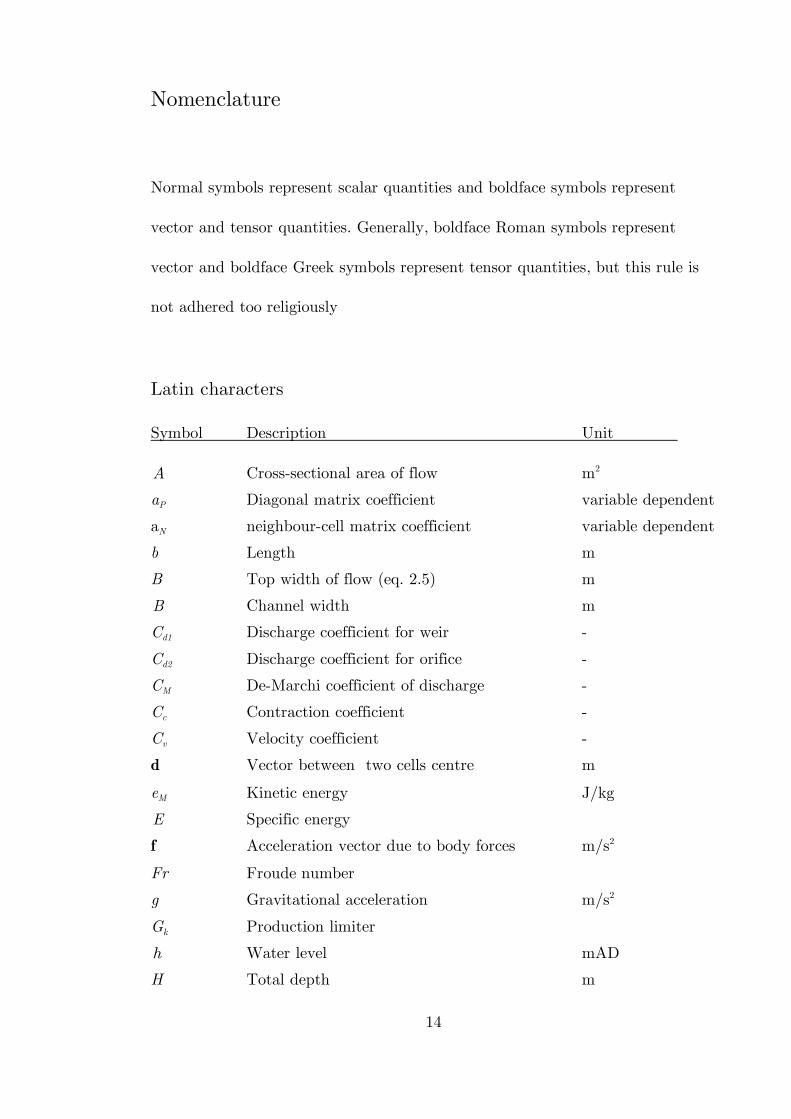
Nomenclature
Normal symbols represent scalar quantities and boldface symbols represent
vector and tensor quantities. Generally, boldface Roman symbols represent
vector and boldface Greek symbols represent tensor quantities, but this rule is
not adhered too religiously
Latin characters
Symbol Description Unit
A Cross-sectional area of flow m2
aP Diagonal matrix coefficient variable dependent
aN neighbour-cell matrix coefficient variable dependent
b Length m
B Top width of flow (eq. 2.5) m
B Channel width m
Cd1 Discharge coefficient for weir -
Cd2 Discharge coefficient for orifice -
CM De-Marchi coefficient of discharge -
Cc Contraction coefficient -
Cv Velocity coefficient -
d Vector between two cells centre m
eM Kinetic energy J/kg
E Specific energy
f Acceleration vector due to body forces m/s2
Fr Froude number
g Gravitational acceleration m/s2
Gk Production limiter
h Water level mAD
H Total depth m
15
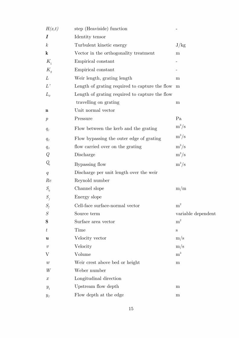
H(x,t) step (Heaviside) function -
I Identity tensor
k Turbulent kinetic energy J/kg
k Vector in the orthogonality treatment m
1K Empirical constant -
2K Empirical constant -
L Weir length, grating length m
L’ Length of grating required to capture the flow m
L0 Length of grating required to capture the flow
travelling on grating m
n Unit normal vector
p Pressure Pa
q1 Flow between the kerb and the grating m3/s
q2 Flow bypassing the outer edge of grating m3/s
q3 flow carried over on the grating m3/s Q Discharge m3/s
bQ Bypassing flow m3/s
q Discharge per unit length over the weir
Re Reynold number
0S Channel slope m/m
fS Energy slope
Sf Cell-face surface-normal vector m2
S Source term variable dependent
S Surface area vector m2
t Time s
u Velocity vector m/s
v Velocity m/s
V Volume m3
w Weir crest above bed or height m
W Weber number
x Longitudinal direction
1y Upstream flow depth m
y2 Flow depth at the edge m
16
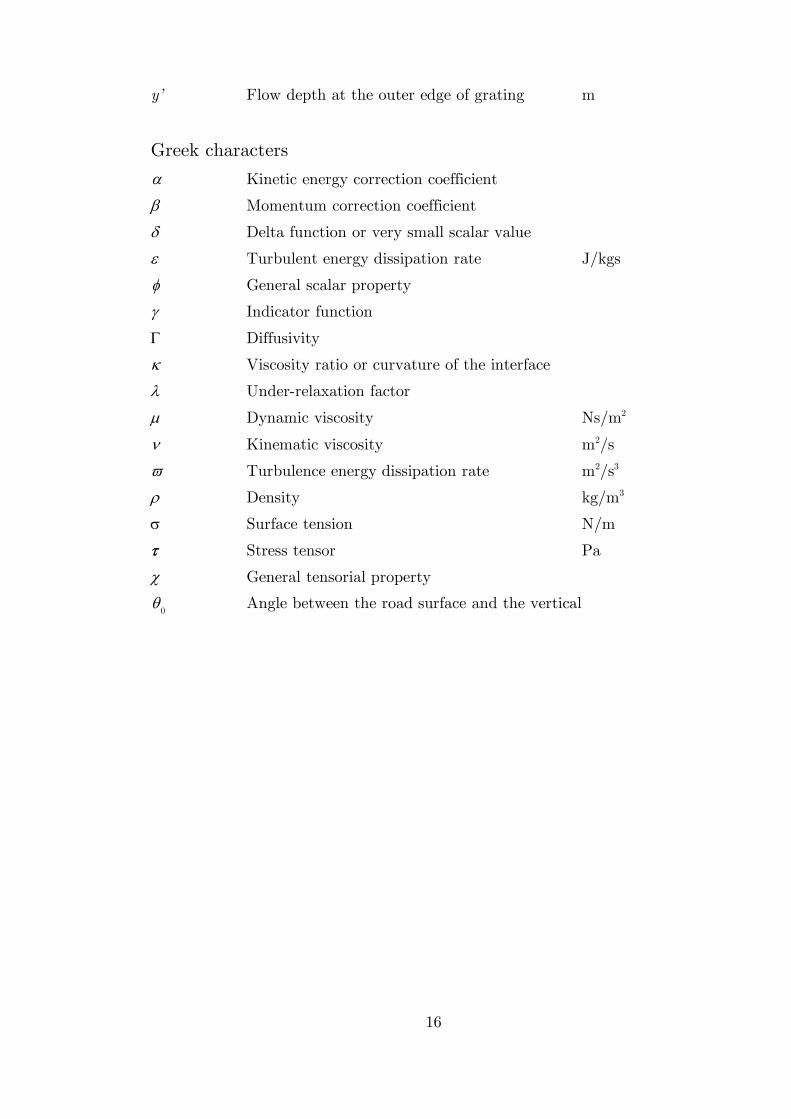
y’ Flow depth at the outer edge of grating m
Greek characters Kinetic energy correction coefficient
Momentum correction coefficient
Delta function or very small scalar value
Turbulent energy dissipation rate J/kgs
General scalar property
Indicator function
Diffusivity
Viscosity ratio or curvature of the interface
Under-relaxation factor
Dynamic viscosity Ns/m2
Kinematic viscosity m2/s
Turbulence energy dissipation rate m2/s3
Density kg/m3
Surface tension N/m
Stress tensor Pa
General tensorial property
0 Angle between the road surface and the vertical
17
Chapter 1
Introduction
Storm water collection and conveyance systems are critical components of urban
drainage systems. Proper design and management of these systems are essential
to minimize flood damage and disruptions in urban areas during storm events.
Runoff water must be captured mainly by gully inlets. To locate and size these
inlets properly, designers need reliable information on their hydraulic
performance. Nowadays frequent flood events reinforce the need for using
accurate models to simulate flooding and help urban drainage engineers. A
source of uncertainty in these models is the lack of understanding of the
complex interactions between the above and below ground drainage systems.
Such knowledge is essential for enhanced calibration and verification of 1D-2D
hydrodynamic modelling approaches (Leandro, et al., 2009). However, general
references in this subject disregard the complexity of the interaction between
these two systems. They assume the inlet capacity is controlled solely by the
inlet type and the flow on the surface (Almedeij & Houghtalen, 2003) or by
gully efficiency (Balmforth, et al., 2006). The geometry of the inlet below
ground is considered irrelevant. The most common way in which this element
has been modelled is either as a weir or as an orifice, or as a combination of
these. However, none of these elements are representative of the real flow
18
conditions. Moreover, the real linking elements include not only the surface
inlet, but also the pipe inlet and its connections, the gully pot and the buried
sewer pipe connections (Djordjevic, 2009).
1.1 Motivation
The Foresight Future Flooding study (Evans, et al., 2004a) (Evans, et al.,
2004b), highlighted the lack of accurate tools and methodologies for the
prediction of the cause and extent of urban flooding, and of urban flood
impacts. The report also promoted the development of an integrated approach
to flood modelling to support accurate analysis of integrated portfolios of flood
management responses. The UK flooding in summer 2007 was a wakeup call to
challenge scientists and experts to face this problem. The need for investment in
developing flood modelling tools became an essential task. There has been
significant development of urban flood modelling tools in last few years. These
models have been developed to interact the flood flows between the above and
below ground drainage systems. The major deficiency in their application relates
to the way in which the flows enter the below ground system through
inlets/gullies on the catchment surface and, subsequently, when the below
ground drainage system is full, how the flows exit through the gullies onto the
catchment surface.
Until recently, drainage system models have assumed that there is a “free”
connection between the urban surface and the below ground system and vice
versa, but it is becoming increasingly evident that this is not the case. In some
19
areas there is a significant lack of gullies whilst at other locations the gullies
may be partially or completely blocked. The way in which these gulley
inlets/outlets are described (free discharge, partially or fully blocked) is
therefore critical to the accurate prediction of the hydraulic performance of the
system. There is a need therefore to better describe the performance of such
types of gulley system commonly found in practice. Such understanding is
essential to improve the crude representation and uncertainty of existing
techniques. This need has also been identified by researchers and the developers
of urban flood risk software.
1.2 Objectives
The overall objective of the research described in this thesis was to improve
understanding of the interaction between above and below ground elements of
urban flood models. The present research focuses on the hydraulics of gully
flows. The aim of this study was divided into a number of specific objectives
which are presented below:
Evaluate the application of CFD modelling for simulating flow into and
from gullies;
Examine flow patterns and flow regimes around the gully;
Develop and test a novel algorithm to link 2D and 3D Computational
Fluid Dynamics models;
Application of CFD modelling to generate new knowledge for improving
urban flood models;
20
Provide a basis of generalizing hydraulic descriptions for gully flow.
1.3 Structure of thesis
This thesis is divided in six chapters including this introduction.
In Chapter 2 a review of relevant literature is provided. The review covers the
main areas of research addressed including grate inlet hydraulics, discharge
coefficient, linking surface and subsurface networks, CFD modelling applied in
urban drainage.
Chapter 3 provides the description of full scale physical experiment (completed
in Sheffield Laboratory) to mimic the hydraulic interaction between the above
and below ground drainage system via gully inlet.
In Chapter 4 the mathematical and numerical models are described. A novel
methodology, based on finite volume discretization, to link the 3D and 2D
domain is proposed.
In Chapter 5 implementation of the proposed model is presented. Both flow into
gully and surcharged gully are investigated with the numerical model.
Conventional and new methods developed for calculation of discharge coefficient
and estimation of bypassing flow rate are presented in this chapter.
In Chapter 6 the key findings of this thesis are summarised and relevant
conclusions are drawn. The novel aspects introduced in this thesis are
highlighted, followed by possible directions of future research to enhance and
extend the methodologies presented.
21
Chapter 2
Previous and Related Studies
An overview of the literature relevant to this study is presented next. In the
first section the studies related to grate inlets are reviewed.
2.1 Grate Inlet
The studies on grate inlets covered multiple interesting fields. Most researchers
were keen to investigate the effectiveness of the grate inlet (Larson, 1947), (Li,
et al., 1951), (Li, et al., 1954), others proposed several potential modifications
on the existing grate inlet designs (Almedeij & Houghtalen, 2003), (Guo, 2000a)
(Guo, 2000b). This section does not attempt to review all of the research and
literature related to the street inlets but focuses on grate inlets without
depression that are located on a gutter.
The literature indicates that there are many factors that contribute to the
performance of a gully inlet:
the type and shape of the grating;
the transversal and longitudinal street slopes;
the width and depth of the approaching flow;
the depth and velocity of flow over the grating;
22
the presence of vortices;
the accumulation of debris.
Depending upon the depth of flow, grate inlets operate under three different
conditions of flow:
1. weir flow;
2. transitional flow, indefinable flow because of vortices and other
disturbances;
3. orifice flow.
The inlet may operate like a weir when the water depth is shallow, or like an
orifice when it is submerged (Guo, 1997) (Guo, 2000a) (Guo, 2000b) (Guo,
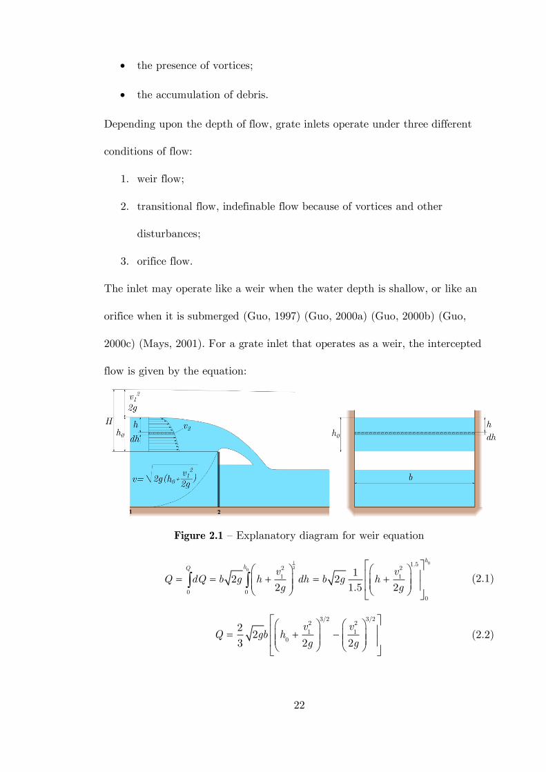
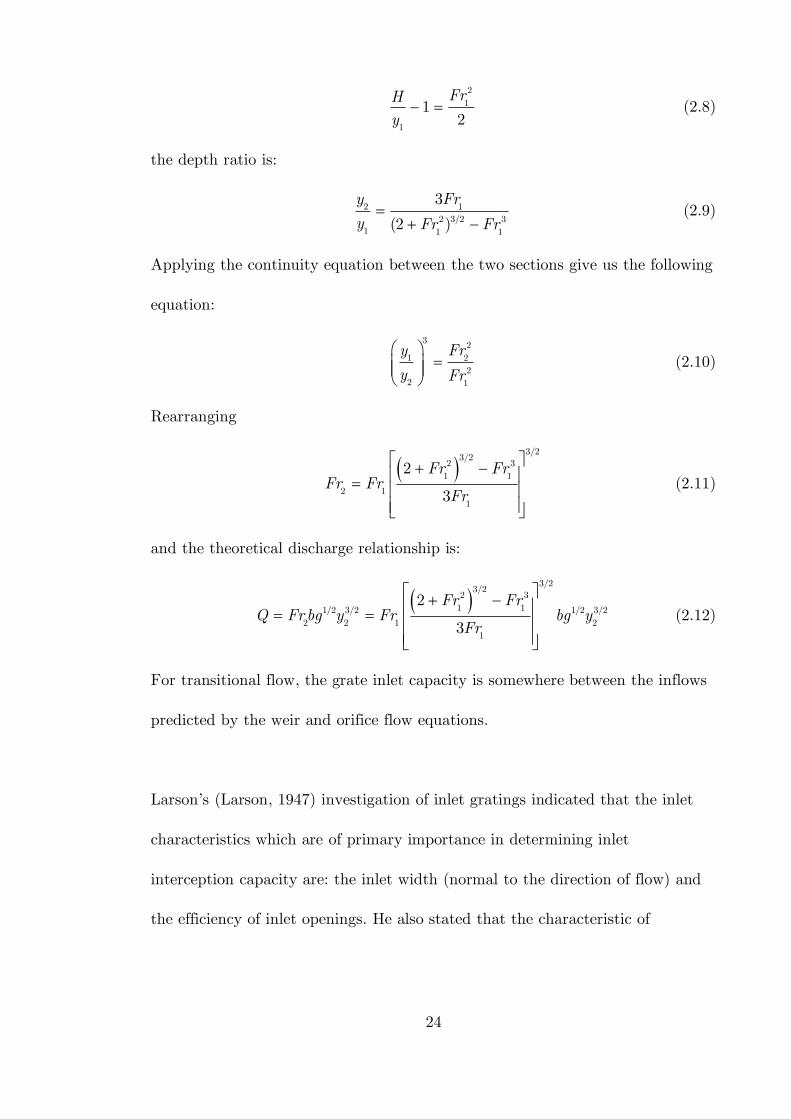
2000c) (Mays, 2001). For a grate inlet that operates as a weir, the intercepted
flow is given by the equation:
Figure 2.1 – Explanatory diagram for weir equation
1 020
1.52 2
1 1
0 00
12 2
2 1.5 2
hhQ v v
Q dQ b g h dh b g hg g
(2.1)
3/2 3/22 2
1 10
22
3 2 2
v vQ gb h
g g
(2.2)
23
where, b is the width of weir, h0 is the water level above weir crest level, v is
flow velocity and g is the gravitational acceleration.
Introducing the discharge coefficient to incorporate the local losses:
3/2 3/22 2
1 11 0
22
3 2 2d
v vQ C gb h
g g
(2.3)
In case of small velocity the term
3/22
1
2
v
g
is negligible or can be included in
discharge coefficient (Cd1), therefore:
3/2
1 1
22
3dQ C gbH (2.4)
The flow over the gully inlet can be assumed to be similar to the flow over the
weir, in which case h0=y1. In accordance with the procedure applied to compute
the discharge: zero pressure distribution, parallel streamlines and neglecting the
contraction of the nappe is assumed:
1
3/2 3/2
10
2 22 ( ) ( )
3
y
c
b gQ C g H z bdz H H y
(2.5)
sC is a contraction coefficient, equal to the ratio between the two cross-section
area, z is the vertical distance measured from reference level. Taking into
account the convergence of streamlines and rearranging the equation leads to:
3/2 3/2211/2 3/2 1/2 3/2
11 1
2 2[ ( ) ]
3
yb gQH H y
ybg y bg y (2.6)
Introducing 1/2 3/2
1 1/Fr Q bg y we obtain:
3/2 3/2
21
1 1 1
2 21
3
y H HFr
y y y
(2.7)
Considering that
24
2
1
1
12
FrH
y (2.8)
the depth ratio is:
2 12 3/2 3
1 1 1
3
(2 )
y Fr
y Fr Fr
(2.9)
Applying the continuity equation between the two sections give us the following
equation:
3 2
1 22
2 1
y Fr
y Fr
(2.10)
Rearranging
3/23/2
2 3
1 1
2 11
2
3
Fr FrFr Fr
Fr
(2.11)
and the theoretical discharge relationship is:
3/23/2
2 31 11/2 3/2 1/2 3/2
2 2 1 21
2
3
Fr FrQ Frbg y Fr bg y
Fr
(2.12)
For transitional flow, the grate inlet capacity is somewhere between the inflows
predicted by the weir and orifice flow equations.
Larson’s (Larson, 1947) investigation of inlet gratings indicated that the inlet
characteristics which are of primary importance in determining inlet
interception capacity are: the inlet width (normal to the direction of flow) and
the efficiency of inlet openings. He also stated that the characteristic of
25
approach flow has a significant effect on efficiency. His tests showed that high
velocities tend to decrease the inlet capacity due to splashing.
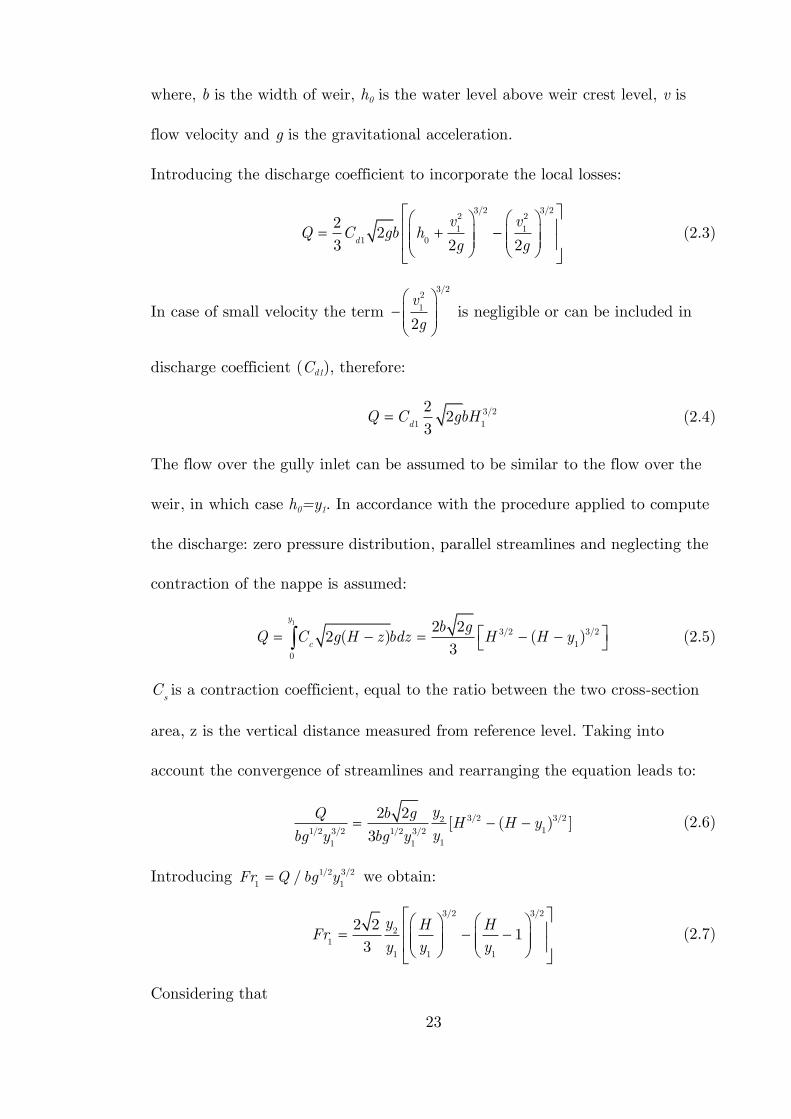
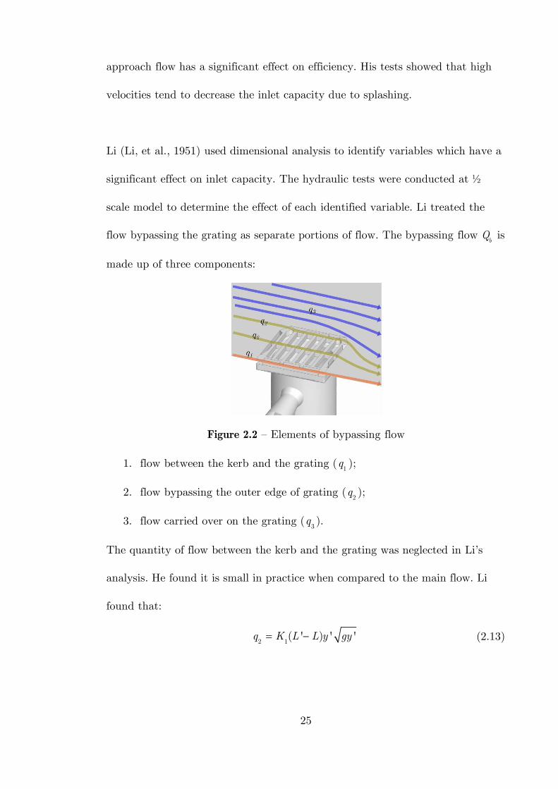
Li (Li, et al., 1951) used dimensional analysis to identify variables which have a
significant effect on inlet capacity. The hydraulic tests were conducted at ½
scale model to determine the effect of each identified variable. Li treated the
flow bypassing the grating as separate portions of flow. The bypassing flow bQ is
made up of three components:
Figure 2.2 – Elements of bypassing flow
1. flow between the kerb and the grating (1q );
2. flow bypassing the outer edge of grating (2q );
3. flow carried over on the grating (3q ).
The quantity of flow between the kerb and the grating was neglected in Li’s
analysis. He found it is small in practice when compared to the main flow. Li
found that:
2 1( ' ) ' 'q K L L y gy (2.13)
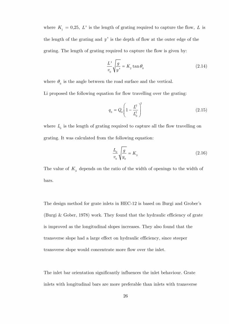
26
where 1K = 0,25, 'L is the length of grating required to capture the flow, L is
the length of the grating and 'y is the depth of flow at the outer edge of the
grating. The length of grating required to capture the flow is given by:
2 0
0
'tan
'
L gK
v y (2.14)
where 0
is the angle between the road surface and the vertical.
Li proposed the following equation for flow travelling over the grating:
22
3 0 2
0
1L
q QL
(2.15)
where 0L is the length of grating required to capture all the flow travelling on
grating. It was calculated from the following equation:
03
0 0
L gK
v y (2.16)
The value of 3K depends on the ratio of the width of openings to the width of
bars.
The design method for grate inlets in HEC-12 is based on Burgi and Grober’s
(Burgi & Gober, 1978) work. They found that the hydraulic efficiency of grate
is improved as the longitudinal slopes increases. They also found that the
transverse slope had a large effect on hydraulic efficiency, since steeper
transverse slope would concentrate more flow over the inlet.
The inlet bar orientation significantly influences the inlet behaviour. Grate
inlets with longitudinal bars are more preferable than inlets with transverse
27
bars. The transverse bars reduce the effectiveness of the grating because they
reduce the effective length of the grating and increase the splashing across the
inlet. The study of John Hopkins University (John Hopkins University, 1956)
showed that short and wide grating is more effective for general street
conditions than long and narrow grating. Bourchard and Towsend (Bourchard
& Towsend, 1984) investigation of inlet bar orientation indicated that inlets
with transverse bars (90°) are the least effective. Inlets with 135° opening
showed good correlation with longitudinal bars for low discharges but less
effective for high discharges. The study involved full scale model with different
inlet patterns, in which the bar orientation were ranged from 0° to 165° at 15°
intervals.
2.2 Discharge Coefficient
Johnson’s study (Johnson, 2000) showed that the important variable governing
discharge over weirs was Ht/w. The use of this variable, coupled with the
inclusion of the weir height in the velocity head, resulted in the formulation of a
single curve rather than a family of curves. He also pointed out that the
importance of the velocity head should not be neglected.
Kindsvater and Carter (Sturm, 2001) proposed that the effect of Reynolds and
Weber number should be included in the discharge equation.
28
Johnson (Johnson, 2000) and Rehbock (Rehbock, 1929) research showed that
the transverse length of the weir has little influence on the discharge coefficient,
and this is valid for surface roughness of the weir as well.
Flow over the grating represents a typical example of spatially varied flow with
decreasing discharge. Several authors proposed equations for spatially varied
flow profile. The dynamic equation of spatially varied flow for over a weir is
0 2
2
31
f
Q dQS S
dxgAdy
dx Q B
gA
(2.17)
Subramanya (Subramanya & Awashty, 1972), El-Khasab and Smith (El-Kashab
& Smith, 1976), Ranga Raju (Ranga Raju, et al., 1979), Hager (Hager, 1987)
and Singh (Singh, et al., 1994) used experimental results to evaluate the
rectangular weir equation. Swamee (Swamee, et al., 1994) developed elementary
discharge coefficients that are related to the discharge through an elementary
strip along the side weir.
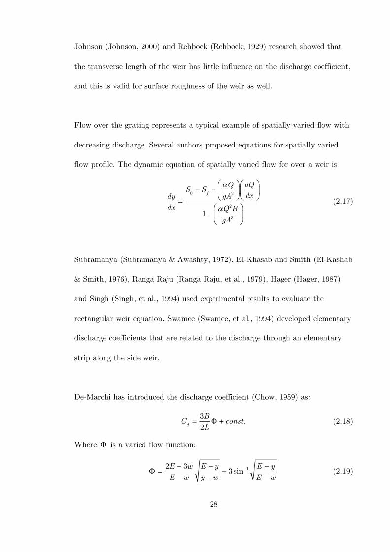
De-Marchi has introduced the discharge coefficient (Chow, 1959) as:
3
.2d
BC const
L (2.18)
Where is a varied flow function:
12 33sin
E w E y E y
E w y w E w
(2.19)
29
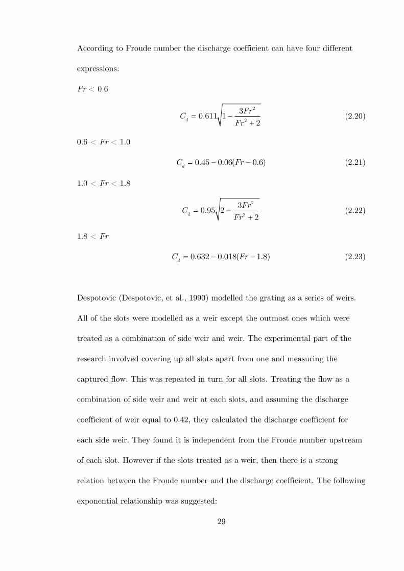
According to Froude number the discharge coefficient can have four different
expressions:
Fr < 0.6
2
2
30.611 1
2d
FrC
Fr
(2.20)
0.6 < Fr < 1.0
0.45 0.06( 0.6)dC Fr (2.21)
1.0 < Fr < 1.8
2
2
30.95 2
2d
FrC
Fr
(2.22)
1.8 < Fr
0.632 0.018( 1.8)dC Fr (2.23)
Despotovic (Despotovic, et al., 1990) modelled the grating as a series of weirs.
All of the slots were modelled as a weir except the outmost ones which were
treated as a combination of side weir and weir. The experimental part of the
research involved covering up all slots apart from one and measuring the
captured flow. This was repeated in turn for all slots. Treating the flow as a
combination of side weir and weir at each slots, and assuming the discharge
coefficient of weir equal to 0.42, they calculated the discharge coefficient for
each side weir. They found it is independent from the Froude number upstream
of each slot. However if the slots treated as a weir, then there is a strong
relation between the Froude number and the discharge coefficient. The following
exponential relationship was suggested:
30
exp( 0.453 0.226)dC Fr (2.24)
Tomanovic (Tomanovic, et al., 1990) applied the above equation for grating in
their study and obtained good results at lower cross-falls and flow rates.
Borghei (Borghei, et al., 1999) conducted more than 250 laboratory tests to find
the influence of the flow hydraulics and the geometric, channel, and weir shapes
on the discharge coefficient. The results show that for subcritical flow the
De-Marchi assumption of constant energy is acceptable. He found that the
De-Marchi discharge coefficient is a function of the upstream Froude number
and the ratios of weir height to upstream depth and weir length to channel
width. Borghei proposed the following equation for calculation of discharge
coefficient:
1
1
0.7 0.48 0.3 0.06M
w LC Fr
y B (2.25)
Matthew (Matthew, 1963) outlined a simple theory which clearly explains the
influence of surface tension, viscosity and streamline geometry on discharge
coefficient. Martino and Ragone (Martino & Ragone, 1984) conducted a
comprehensive study on the effect of surface tension and viscosity on discharge
coefficient.
The study stated that an increase in the influence of surface tension (or
reduction in Weber number) will engender an increment in the coefficient of
contraction exceeding the decrement in that of velocity, but only for values of
Weber number above a certain threshold, which is a function of both slot
31
breadth and the head. Below the threshold the decrements in the velocity
coefficient exceed the increments of the contraction coefficient due to viscosity
and to surface tension. Increase in the influence of viscosity (or reduction in
Reynolds number) implies an increment in the contraction coefficient, always
prevailing over the decrement in that velocity arising from the loss of head due
to viscous drag.
Similarly to Martino’s research the models proposed by Kindsvater (Kindsvater
& Carter, 1957), Getti (Ghetti, 1966), Gavis (Gavis, 1964), Linquist (Linquist,
1929), Datei (Datei, 1966) and Sarginson (Sarginson, 1972) give valuable
information on the effect of surface tension and viscosity on discharge
coefficient.
De Martino’s (De Martino & Ragone, 1979) study concluded that both viscosity
and surface tension have each opposite effects on the contraction coefficient Ce
and velocity coefficient Cv. The investigation concentrated on Reynolds and
Weber numbers and found that reduction in the Reynolds number accompanied
by an increase in Ce and decrease in Cv. Similar effects are also caused by an
increase in surface tension (a decrease in the Weber number). The fact that Ce
and Cv tend to increase and decrease respectively, for an increase in either
viscosity or surface tension accounts for the possible arising of conditions when,
for values of the Reynolds and Weber numbers below a certain threshold (i.e..
for the slots investigated, for low head values), the reductions in the velocity

32
coefficient prevail on the increments in the contraction coefficient, so that the
discharge coefficient (the product of Ce and Cv) will tend to decrease.
The existence of such conditions was also confirmed by Swift (Swift, 1926) and
surmised by Sarpkaya (Sarpkaya, 1958) as well.
Honar (Honar & Keshavarzi, 2008) conducted more than 90 laboratory tests to
develop a model for estimation of discharge coefficient in rounded-edge entrance
shape and find the influence of non-dimensional hydraulic parameters on the
discharge coefficient. It was found that under subcritical flow condition the
rounded-edge entrance discharges 10% more flow rate than the squared edge
entrance.
2.3 Linking surface and sub-surface networks
The interaction between surface and subsurface drainage network is
complicated, while knowledge of their hydraulic characteristics is very limited.
A general hydraulic description is yet to be derived. Current practices of gully
designs mostly rely on empirical relations from a limited number of
experimental studies. Further study to advance the knowledge of gully
hydraulics is necessary and valuable, especially when existing drainage systems
are challenged today by a combination of urban growth, ageing of sewers and
climate change.
Poor knowledge of the hydraulic behaviour of surface drainage structures could
produce unreliable simulations from storm water management models (Russo, et
33
al., 2005) (Gomez & Russo, 2011). Kidd and Helliwell (1977) described the
urban runoff process as a two-phase phenomenon including a surface phase and
an underground phase. They recognized the complex interactions between these
two phases and stated “there is no clear-cut interface between the two phases”.
Inasmuch as the inlet efficiency governs the amount of water that can enter the
drainage system, the above surface and below surface elements cannot be
considered separately. Nowadays the lack of knowledge about the hydraulic
behaviour of these types of structures has not been fully overcome (Gomez &
Russo, 2011).
Three different linkage types are available for dynamically linking the 1D and
2D storm water management models:
1. Point to point link: is a standard link type, coupling between a
computational point in the 1D model and a computational point in the
2D model. It can be used to couple upstream river branch to a
downstream flood plain.
2. Lateral link: couples the 1D model with 2D domain over a part of the
river system. The flow is described through a weir equation in each
linked grid point. This type of link can be used for simulation of
overtopping levees
3. Structure link: uses 1D model in a 2D domain to model flow through a
structure, which is –usually- defined in the 1D model. This type of link is
useful for modelling small features which cannot be adequately resolved
using the typical grid size of the 2D domain.
34
With the increasing requirements for integrated modelling, particularly 1D to
2D linking for surface water flooding, a need has arisen to provide a unit to
simulate discharge through a manhole or gully from a surcharged culvert.
In ISIS (www.halcrow.com/isis) the manhole outlet can be connected to a
dummy boundary unit for linking to TUFLOW (www.tuflow.com), or to a
reservoir to represent overland storage. The manhole unit can also incorporate
an energy loss term, governed by Bernoulli's equation. TUFLOW has a similar
connection to ESTRY as it has to ISIS.
HEC-HMS (www.hec.usace.army.mil/software/hec-hms/)was designed to
simulate rainfall-runoff process. The inlet can be represented as a flow diversion
and its hydraulic efficiency can be described with the approaching flow –
intercepted flow curve.
SWMM (Storm Water Management Model) is a dynamic rainfall-runoff
simulation model (www.epa.gov./athens/wwqtsc/html/swmm.html). The
routing part of the software transports the runoff through a system of pipes and
channels using kinematic or dynamic wave. The hydraulic behaviour of the
street is described as an open channel and the inlet is characterised as a divider
node describe by hydraulic efficiency data. This is represented by the ratio
between total discharge approaching to the inlet and captured flow.
MOUSE (www.dhisoftware.com) is a comprehensive surface runoff, open
channel flow and pipe flow modelling package. The behaviour of street inlets
can be described with flow depth using the weir equation.
35
Many different techniques exist to connect the 1D and 2D domains via gullies or
manholes. The most frequently used representation of street inlets in numerical
models can be summarized as:
Diversion elements characterized by inflow-captured flow table;
Diver nodes characterized by inflow-outflow table;
Weir equation;
Orifice equation;
Combination of orifice and weir equation;
Efficiency-head curve.
2.4 CFD Modelling
Due to the limitation with experimental investigation numerical models seem to
be a reliable alternative for studying gully hydraulic performance. Compared to
conventional measurements methods, a significant advantage of Computational
Fluid Dynamics (CFD) model is the reduction in both the time and cost that
are typically required to investigate gully flow. Another important factor, that
it can be applied to different environmental condition including those that could
not be modelled under laboratory conditions. It has been widely accepted that a
good numerical model can be complementary to experimental tests. CFD is a
tool that has tended to be used in “high-tech” industries. However,
computational power has become more affordable and CFD is getting more
frequently used in urban drainage. The published information shows that CFD
36
is most commonly applied in order to gain detailed design knowledge or to
evaluate structural or operational variables (Jarman, et al., 2008).
Huang (Huang, et al., 2002) and Shakibainia (Shakibainia, et al., 2010) used
three-dimensional models to compute flow characteristics in 90 junction and
showed that most flow structures observed experimentally were accurately
simulated.
Fang (Fang, et al., 2010) investigated the efficiency of curb inlets using three-
dimensional CFD model. The model used a finite-volume-finite-difference
method to discretise the 3D Reynolds Averaged Navier-Stokes equations in fixed
Eulerian rectangular grid system. Simulation runs were performed for 1.52 m
and 4.56 m opening at various longitudinal and cross slopes. Simulated
intercepted flow rate agreed well with laboratory test. The simulation results
were used to develop a linear regression equation between inlet efficiency and
water spread.
Stovin (Stovin & Saul, 1998), Cullivan (Cullivan, et al., 2004) and Schuetz
(Schuetz, et al., n.d.) have used CFD technique to investigate particle tracking
in order to assess the separation efficiency in CSO tanks.
Fach (Fach, et al., 2009) study is focused on the development of rating curves
exemplarily for CSO structures using three-dimensional CFD model. The study
showed that discharge determined by using the standard weir equation together
with sonic water depth measurement can significantly differ from the discharge
based on CFD simulation. Especially, for side weirs which did not correspond to
37
the standard weir layout, the results from the CFD model were closer to the
reality than the simplified standard weir equation.
The prediction of the water surface profile is fundamental in urban drainage
modelling. However this is absent from the majority of the studies in which the
free surface was assumed as flat and fixed. Jarman et al (Jarman, et al., 2008)
reviewed CFD studies where water surface profiles were not predicted as a part
of the solution process. The free surface was approximated by a fixed, horizontal
frictionless boundary, predefined as part of model geometry. The investigated
models were concerned with the application of CFD for engineering objectives
rather than with the development of modelling methodology. The investigation
concluded that this type of approach is reducing the computational effort but is
not always appropriate.
A similar approach in numerical simulation of free surface flow is when the
water surface is replaced by a rigid lid (Mignot, et al., 2012). This is valid only
if the free surface does not change much along the domain. In the case of this
study the rigid lid approximation likely introduced nonphysical errors.
Ismail and Nikraz (Ismail & Nikraz, 2008) conducted an experimental and
numerical analysis to establish the hydraulic characteristics and pollution
removal efficiency of the cylindrical screen of VersaTrap. It has been designed
to remove suspended solids, floatables and sediments from the storm water and
to prevent re-entrainment. A three-dimensional model was constructed using
tetrahedral meshes comprising of 268000 computational cells. Inlet flow rates

38
(11, 13 and 20 l/s) were defined by uniform velocities across the inlet plane.
System outlets were defined with a pressure outlet corresponding to atmospheric
pressure, representing a free outflow. The VOF model was used to determine
the hydraulic characteristics and Eulerian-Eulerian model was used to obtain
the efficiency of the system. The simulated peak flow was similar to the
experimental results within an error of 22%.
More literature on CFD modelling will be reviewed when CFD methods are
introduced with more detail in Chapter 4.
2.5 Conclusion
Urban storm water collection and conveyance systems are critical components of
the urban drainage. Proper design of these systems is essential to minimize flood
damage and disruptions in urban areas during storm events. Excess water must
be captured mainly by gully inlets. To locate and size these inlets properly,
designers need reliable information on their hydraulic performance.
Despite of many theoretical and experimental studies carried out on weir,
orifice, free overfall, manhole and gully grating the flow calculation for gratings
has not been completely solved. As discussed above the general references
disregard the interaction between the above and below ground elements of
linked 2D/1D or 1D model. None of the expressions presented this chapter are
directly valid for modelling the link between surface and sub-surface flow. Most
39
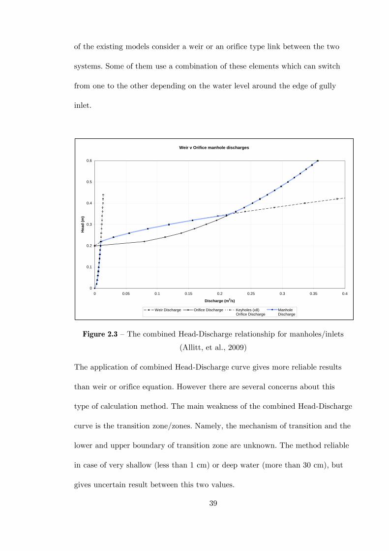
of the existing models consider a weir or an orifice type link between the two
systems. Some of them use a combination of these elements which can switch
from one to the other depending on the water level around the edge of gully
inlet.
Figure 2.3 – The combined Head-Discharge relationship for manholes/inlets
(Allitt, et al., 2009)
The application of combined Head-Discharge curve gives more reliable results
than weir or orifice equation. However there are several concerns about this
type of calculation method. The main weakness of the combined Head-Discharge
curve is the transition zone/zones. Namely, the mechanism of transition and the
lower and upper boundary of transition zone are unknown. The method reliable
in case of very shallow (less than 1 cm) or deep water (more than 30 cm), but
gives uncertain result between this two values.
Weir v Orifice manhole discharges
0
0.1
0.2
0.3
0.4
0.5
0.6
0 0.05 0.1 0.15 0.2 0.25 0.3 0.35 0.4
Discharge (m2/s)
He
ad
(m
)
Weir Discharge Orifice Discharge Keyholes (x8)Orifice Discharge
ManholeDischarge
40
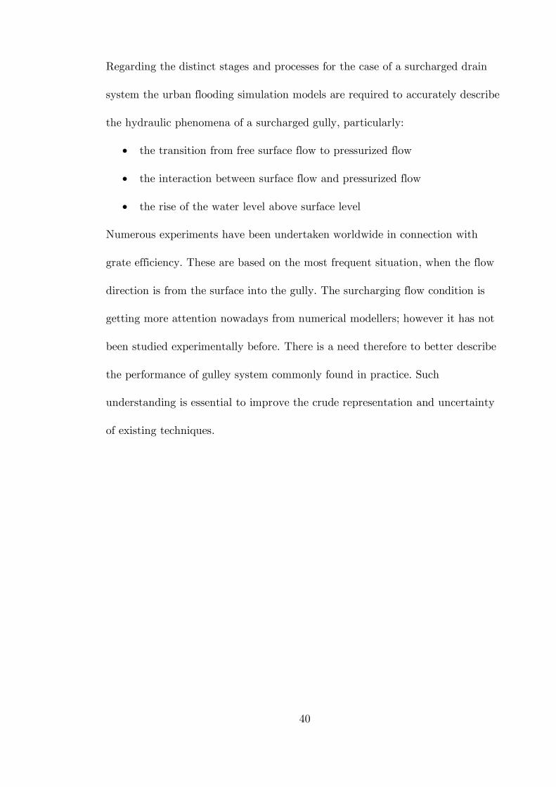
Regarding the distinct stages and processes for the case of a surcharged drain
system the urban flooding simulation models are required to accurately describe
the hydraulic phenomena of a surcharged gully, particularly:
the transition from free surface flow to pressurized flow
the interaction between surface flow and pressurized flow
the rise of the water level above surface level
Numerous experiments have been undertaken worldwide in connection with
grate efficiency. These are based on the most frequent situation, when the flow
direction is from the surface into the gully. The surcharging flow condition is
getting more attention nowadays from numerical modellers; however it has not
been studied experimentally before. There is a need therefore to better describe
the performance of gulley system commonly found in practice. Such
understanding is essential to improve the crude representation and uncertainty
of existing techniques.
41
Chapter 3
Description of Physical Experiments completed in
the Sheffield Laboratory
A full scale laboratory system has been built at the Water Engineering
Laboratory of University of Sheffield to mimic the hydraulic interaction between
the above and below ground drainage system via a gully inlet. The physical
experiments are not the subject of this thesis but they are used to test the CFD
modelling approach; therefore they are described here without too much detail.
A comprehensive overview of the physical experiments and analysis of results is
given by Sabtu (Sabtu, 2012).
3.1 Experimental rig
3.1.1 Testing platform
The testing platform is a 4.27 m long and 1.83 m wide rectangular area with
inlet and outlet tanks of either end of the platform that are each equipped with
sluice gates to control the flow rate onto the testing platform. Both the outlet
tank and the outflow from the gully are connected to a measuring tank which
allows flow rate measurements to be taken. The dimension for the inlet and
outlet tank itself is 2.44 m x 0.61 m. The flow for this system is provided by an
overhead tank and is circulated through the entire system before being
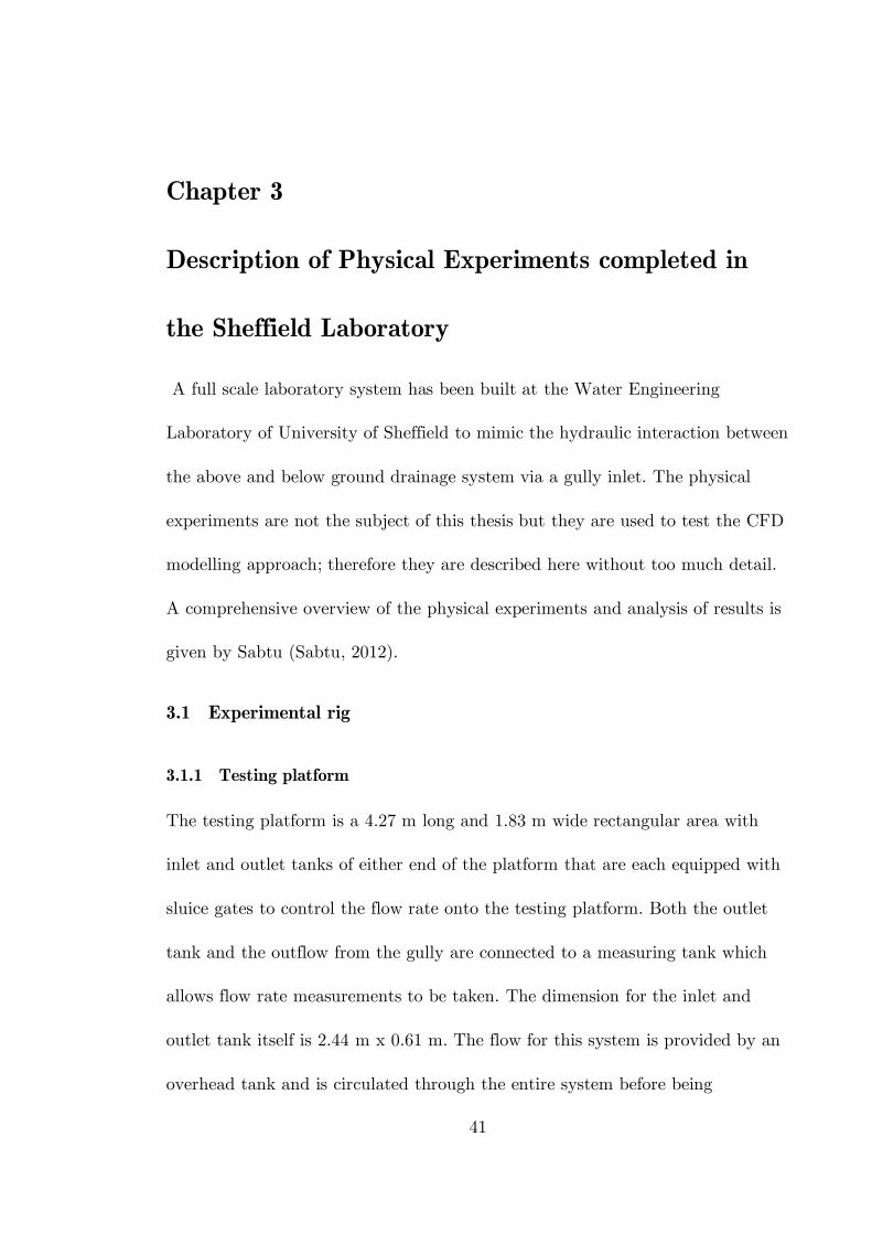
42
transferred into a sump to be pumped back to the overhead tank again (Sabtu,
2012).
Figure 3.1 – Experimental rig (viewed from downstream, gully left)
The testing platform was designed as a flatbed representing non-sloping road
conditions (Figure 3.1). Longitudinal slopes were later incorporated. For sloping
tests, the width of the testing platform has been halved (Figure 3.2) due to the
difficulty of depth measurement of very shallow flow.
Figure 3.2 – Experimental rig for sloping conditions
43
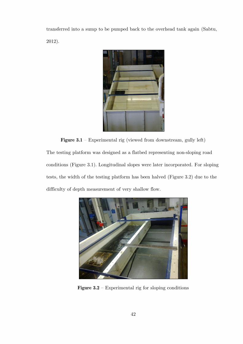
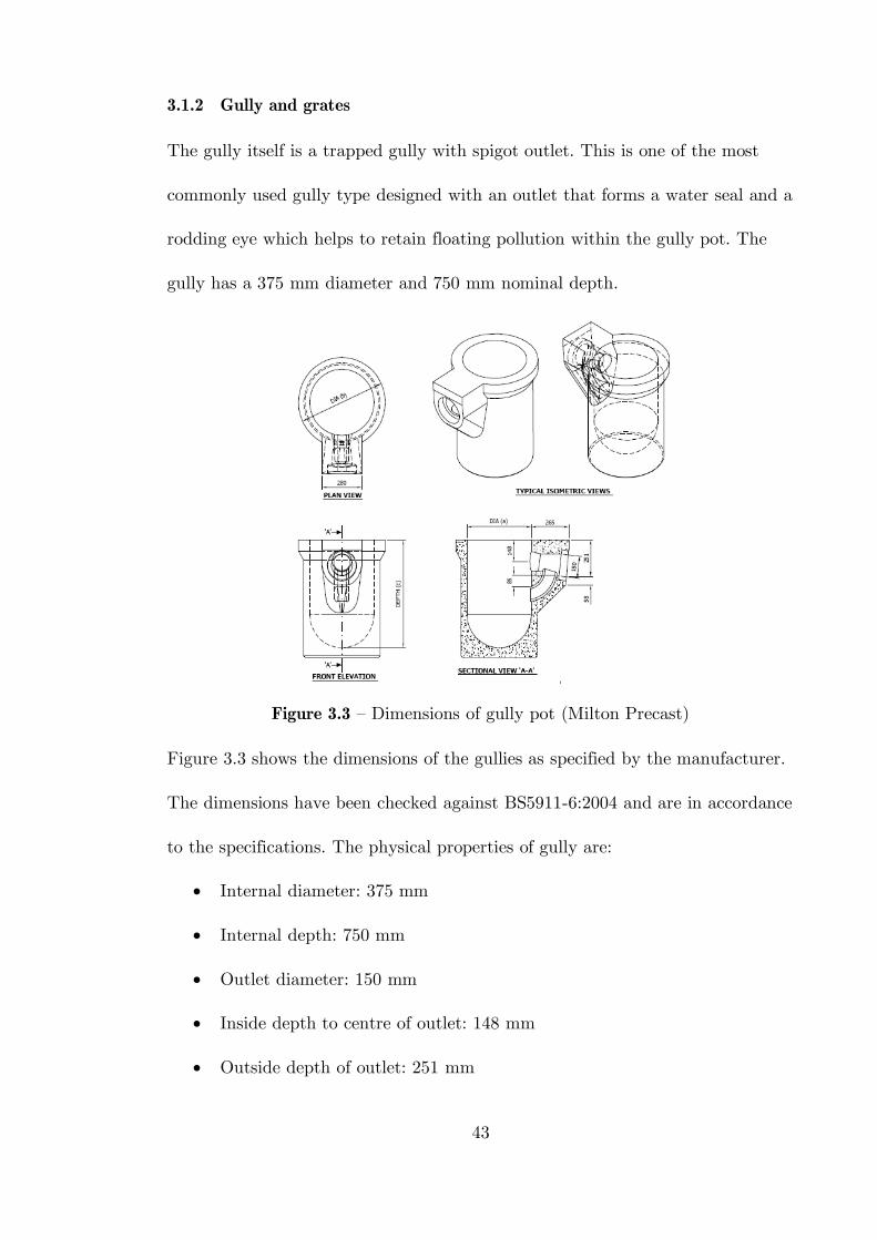
3.1.2 Gully and grates
The gully itself is a trapped gully with spigot outlet. This is one of the most
commonly used gully type designed with an outlet that forms a water seal and a
rodding eye which helps to retain floating pollution within the gully pot. The
gully has a 375 mm diameter and 750 mm nominal depth.
Figure 3.3 – Dimensions of gully pot (Milton Precast)
Figure 3.3 shows the dimensions of the gullies as specified by the manufacturer.
The dimensions have been checked against BS5911-6:2004 and are in accordance
to the specifications. The physical properties of gully are:
Internal diameter: 375 mm
Internal depth: 750 mm
Outlet diameter: 150 mm
Inside depth to centre of outlet: 148 mm
Outside depth of outlet: 251 mm
44
flow direction
Dimension of riser: 85 mm
Depth of water seal: 85 mm
Weight: 180 kg
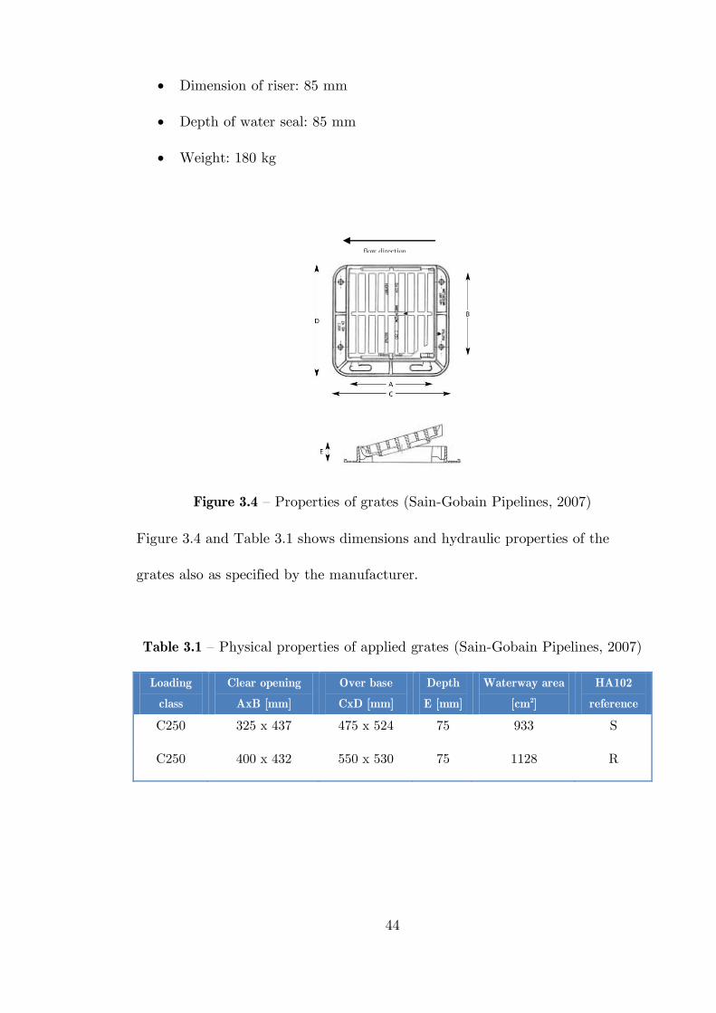
Figure 3.4 – Properties of grates (Sain-Gobain Pipelines, 2007)
Figure 3.4 and Table 3.1 shows dimensions and hydraulic properties of the
grates also as specified by the manufacturer.
Table 3.1 – Physical properties of applied grates (Sain-Gobain Pipelines, 2007)
Loading
class
Clear opening
AxB [mm]
Over base
CxD [mm]
Depth
E [mm]
Waterway area
[cm2]
HA102
reference
C250 325 x 437 475 x 524 75 933 S
C250 400 x 432 550 x 530 75 1128 R
45
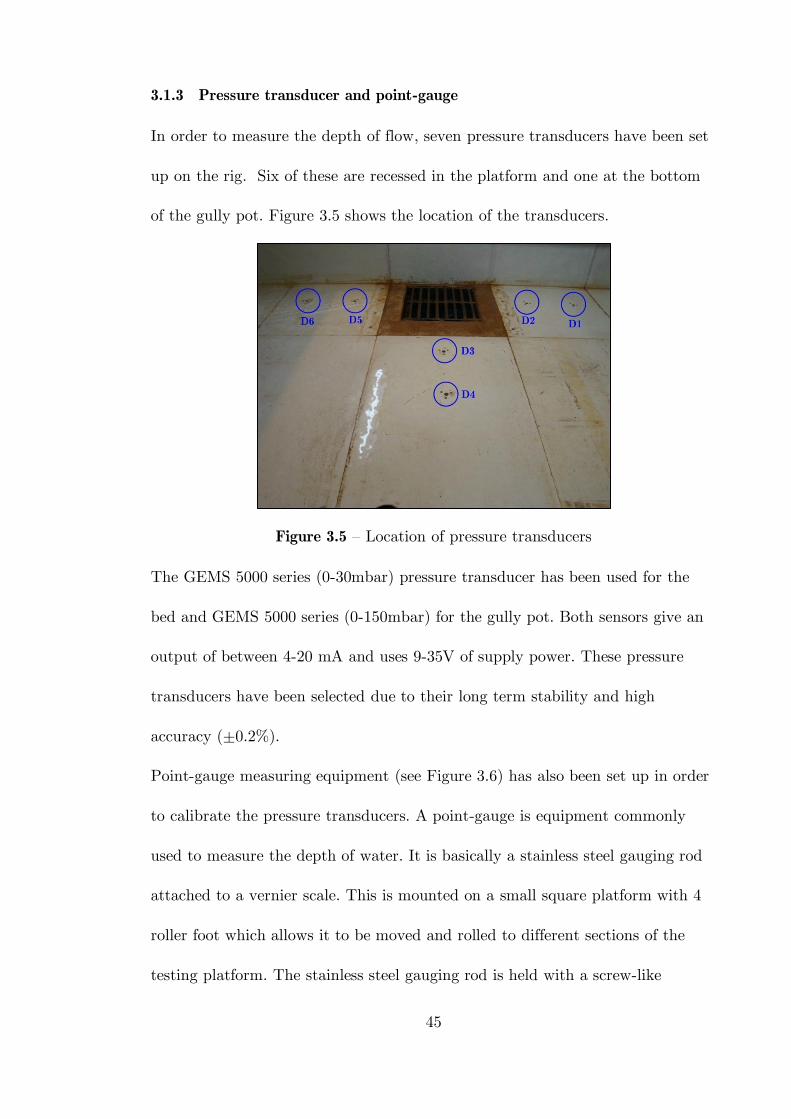
3.1.3 Pressure transducer and point-gauge
In order to measure the depth of flow, seven pressure transducers have been set
up on the rig. Six of these are recessed in the platform and one at the bottom
of the gully pot. Figure 3.5 shows the location of the transducers.
Figure 3.5 – Location of pressure transducers
The GEMS 5000 series (0-30mbar) pressure transducer has been used for the
bed and GEMS 5000 series (0-150mbar) for the gully pot. Both sensors give an
output of between 4-20 mA and uses 9-35V of supply power. These pressure
transducers have been selected due to their long term stability and high
accuracy (±0.2%).
Point-gauge measuring equipment (see Figure 3.6) has also been set up in order
to calibrate the pressure transducers. A point-gauge is equipment commonly
used to measure the depth of water. It is basically a stainless steel gauging rod
attached to a vernier scale. This is mounted on a small square platform with 4
roller foot which allows it to be moved and rolled to different sections of the
testing platform. The stainless steel gauging rod is held with a screw-like
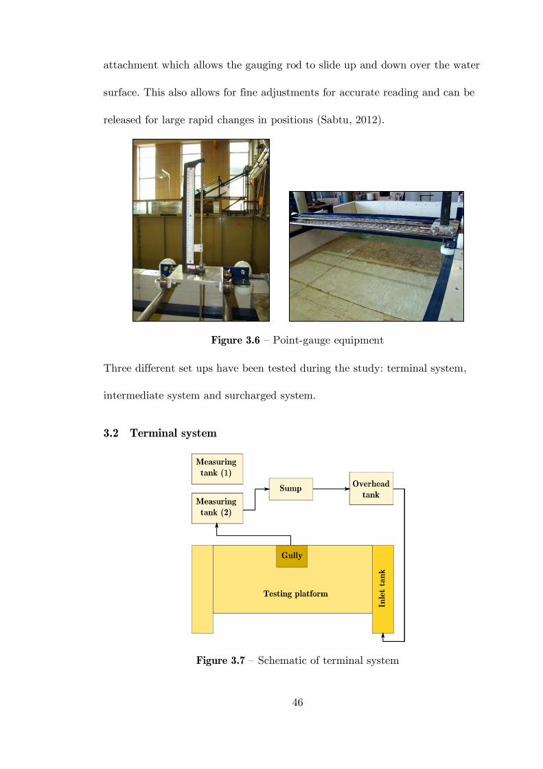
46
attachment which allows the gauging rod to slide up and down over the water
surface. This also allows for fine adjustments for accurate reading and can be
released for large rapid changes in positions (Sabtu, 2012).
Figure 3.6 – Point-gauge equipment
Three different set ups have been tested during the study: terminal system,
intermediate system and surcharged system.
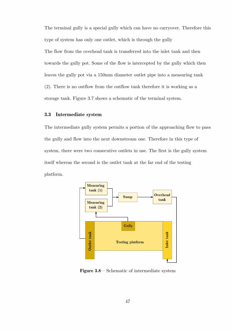
3.2 Terminal system
Figure 3.7 – Schematic of terminal system
47
The terminal gully is a special gully which can have no carryover. Therefore this
type of system has only one outlet, which is through the gully
The flow from the overhead tank is transferred into the inlet tank and then
towards the gully pot. Some of the flow is intercepted by the gully which then
leaves the gully pot via a 150mm diameter outlet pipe into a measuring tank
(2). There is no outflow from the outflow tank therefore it is working as a
storage tank. Figure 3.7 shows a schematic of the terminal system.
3.3 Intermediate system
The intermediate gully system permits a portion of the approaching flow to pass
the gully and flow into the next downstream one. Therefore in this type of
system, there were two consecutive outlets in use. The first is the gully system
itself whereas the second is the outlet tank at the far end of the testing
platform.
Figure 3.8 – Schematic of intermediate system
48
The basic of the system is the same as a terminal system where the only
difference is that the bypassed flow is not passed back onto the testing platform.
Instead, it is collected separately in measuring tank (1) (Sabtu, 2012). Figure
3.8 shows the schematics of the intermediate system.
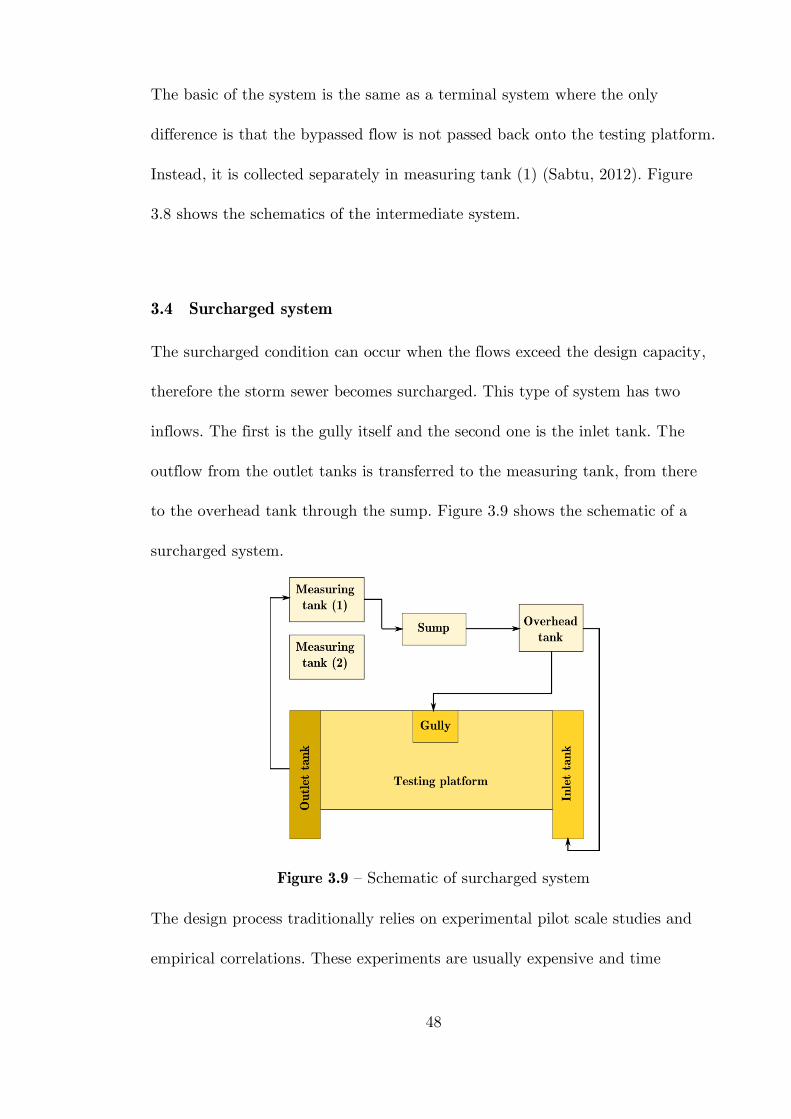
3.4 Surcharged system
The surcharged condition can occur when the flows exceed the design capacity,
therefore the storm sewer becomes surcharged. This type of system has two
inflows. The first is the gully itself and the second one is the inlet tank. The
outflow from the outlet tanks is transferred to the measuring tank, from there
to the overhead tank through the sump. Figure 3.9 shows the schematic of a
surcharged system.
Figure 3.9 – Schematic of surcharged system
The design process traditionally relies on experimental pilot scale studies and
empirical correlations. These experiments are usually expensive and time
49
consuming. Furthermore, the use of pilot scale studies requires the use of scaling
laws to the full-size plant, which may not be well established. In addition the
disruption caused by the installation of the measuring device is often
intolerable.
3.5 Testing protocol
As a first step of the experimental test the transducers were installed and
calibrated. After the calibration the rig was tested without grate later with
grates. Terminal, intermediate and surcharge conditions were tested with 0%
longitudinal and 0% cross-slopes. After the first phase of experimental tests the
rig has been modified: (a) 1:30 longitudinal slop was introduced, (b) rig width
has been halved. The testing protocol established the following conditions:
Total discharge approaching to inlet – Terminal system: 15 l/s, 21 l/s,
26 l/s, 30 l/s, 33 and 36 l/s;
Total discharge approaching to inlet – Intermediate system: 6.0 l/s,
10.5 l/s, 19.9 l/s, 23.8 l/s, 26.9 l/s, 29.6 l/s, 33 l/s;
Surcharging discharge: 1 l/s, 3 l/s, 5 l/s, 10 l/s and 14 l/s;
Longitudinal slope: flat and 1:100;
Cross-slope: flat and 1:30;
Gratings: without grate, Waterflow “S” and Waterflow “R”;
Other condition: with rodding eye and without rodding eye.
50
Chapter 4
CFD Modelling
Free surface flows appear nowadays in many engineering and mathematical
problem. In the last few years many numerical methods have been developed for
the simulation of free-surface flows. A free surface is an interface between a
liquid and a gas in which the gas can only apply a pressure on the liquid. Free
surface flow is an especially difficult class of flows with moving boundaries. The
position of the boundary is known only at the beginning of simulation, its
location at later times has to be determined as part of the solution procedure.
The flow of immiscible fluids can be divided into three groups based on the
interfacial structures: (1) segregated flow, (2) mixed flow and (3) dispersed flow.
This study deals with the segregated type flow. Three different free surface
computation methodologies can be distinguished in modelling of segregated flow,
each of which treats the interfacial jump in a different way (Ferziger & Peric,
1996), (Ubbink, 1997):
1) Interface tracking methods: interface is represented and tracked explicitly
either by marking it with special marker points, or by attaching it to a mesh
surface which is forced to move with the interface.

51
a) Mesh based tracking:
i) Moving mesh method: directly align the phase interface with the edges
of computation mesh cells, which then distracts as the interface
evolves;
ii) Front tracking method: the interface is represented by an additional
two dimensional mesh being superimposed on a fixed three
dimensional mesh;
b) Marker based tracking: the interface is tracked by directly marking it
using massless marker particles;
2) Interface capturing methods: either side of the interface are marked with
massless particles or an indicator function. This class can be divided into
two sub-classes:
a) Marker based capturing: the interface is captured by marker particles
attached to one of the phases in order to gather information about
interfacial morphology from their distribution in the phase volume;
b) Indicator based capturing: a scalar indicator function is used to
distinguish between two different fluids. The indicator function can be
either a scalar step function representing the volume fraction of the space
occupied by one of the fluids (Volume of Fluid) or a smooth function
(Level Set) encompassing a pre-specified iso-surface which identifies the
interface. Two main approaches can be distinguished in indicator based
capturing:
52
i) Single fluid (mixture) approach: the two phases treated as a mixture
having one velocity and pressure. Material properties like viscosities
and densities are taken into account as mixture quantities. This
approach enforces particular properties within the phase, while
fostering a smooth transition across the interface.
ii) Two fluid approach: opposite to single fluid approach the two phases
are treated separately, both having its own velocity and pressure
field. A field belong to one of the phases is consistently transferred to
a fictitious field using the indicator parameter.
3) Hybrid methods: apply elements from both interface capturing and interface
tracking methods. Many combination of above mentioned approaches have
been developed in last decade with the aim of improving deficiencies of the
phase modelling approach.
4.1 Interface capturing methods
The interface capturing methods use an Eulerian mesh, which is fixed in space.
In contrast to interface tracking these approaches do not define the interface as
a sharp boundary as the exact position of the interface is not known explicitly;
therefore special techniques need to be applied to capture the interface. This is
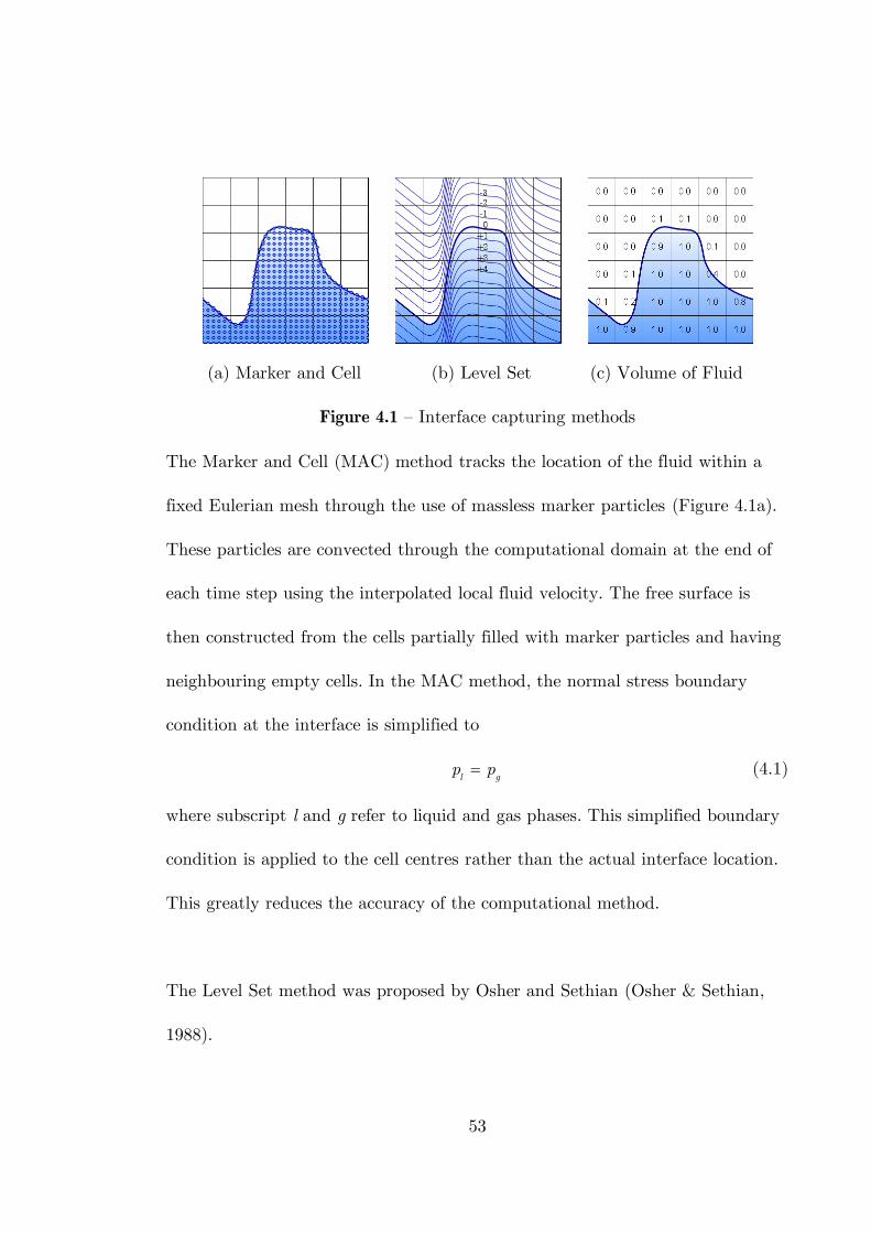
commonly achieved with the following methods (Figure 4.1):
Marker and Cell method
Level Set function
Volume of Fluid method
53
(a) Marker and Cell (b) Level Set (c) Volume of Fluid
Figure 4.1 – Interface capturing methods
The Marker and Cell (MAC) method tracks the location of the fluid within a
fixed Eulerian mesh through the use of massless marker particles (Figure 4.1a).
These particles are convected through the computational domain at the end of
each time step using the interpolated local fluid velocity. The free surface is
then constructed from the cells partially filled with marker particles and having
neighbouring empty cells. In the MAC method, the normal stress boundary
condition at the interface is simplified to
l gp p (4.1)
where subscript l and g refer to liquid and gas phases. This simplified boundary
condition is applied to the cell centres rather than the actual interface location.
This greatly reduces the accuracy of the computational method.
The Level Set method was proposed by Osher and Sethian (Osher & Sethian,
1988).
54
A continuous function is initialized throughout the computational domain as
signed distance from the interface. The function is positive in one phase and
negative in the other. The zero level represents the free surface (Figure 4.1b).
The movement of the interface is calculated by solving the transport equation
for the level set function:
0t
v (4.2)
This equation is derived from the assumption that each particle of liquid moves
with the liquid velocity along the characteristic curves. In the Level Set
approach (4.2) is transformed by setting N
v v to obtain a Hamilton-
Jacobi equation:
0Nt
v (4.3)
where vN is the normal velocity along the gradient . Many numerical
algorithms have been developed to solve (4.3). The most used algorithms are
the ENO (Essentially Non-Oscillatory) and WENO (Weighted Essentially Non-
Oscillatory) introduced by Osher and Sethian (Osher & Sethian, 1988) and
modified by Jiang (Jiang & Peng, 2000) and Croce (Croce, et al., 2004).
The well known drawbacks of the Level Set approach are the degeneration of
and that the method is not mass conservative. Therefore it requires a re-
initialization procedure in every time step to keep the accuracy of
approximation of the interface.
55
The MAC method has evolved into the Volume of Fluid (VOF) method which
can be looked upon as the limit when the number of marker particle becomes
infinite. The original VOF method was proposed by Hirt and Nichols (Hirt &
Nichols, 1981) and represents a compressive scheme with the donor-acceptor
technique for the approximation of fluxes to be advected through cell faces and
it reconstructs the interface as a piecewise constant line segments aligned with
the mesh. The VOF belongs to the Eulerian methods and is based on a scalar
indicator function. The value of the indicator function is equal to one if the cell
is full with fluid, while a zero value would indicate that the cell contained no
fluid (Figure 4.1c). The cells with values between one and zero must contain the
free surface.
Volume of Fluid method is perhaps the most widely used method for free
surface flows despite the difficulties which have to be overcome, namely: how to
advect the interface without diffusing, dispersing or wrinkling it (Ubbink & Issa,
1999). The computation of curvature is difficult, because it involves the
derivitives at the interface of the non-smooth function. The advection of the
characteristic function introduces numerical diffusion which is results in a
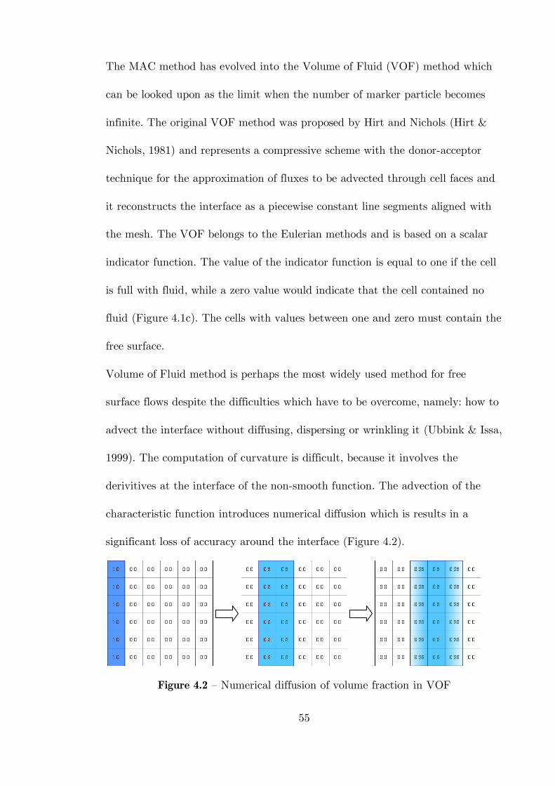
significant loss of accuracy around the interface (Figure 4.2).
Figure 4.2 – Numerical diffusion of volume fraction in VOF
56
Numerous techniques have been investigated to reduce the numerical diffusion.
One of the most common is the Simple Line Interface Calculation (SLIC)
proposed by Noh and Woodward (Noh & Woodward, 1976). This technique
approximates the interface in each cell as a line parallel with one of the
coordinate axes. The direction and position of the line are deduced from the
values of the volume fraction of liquid in the cell and certain neighbourhood of
the cell considered. Another commonly used technique is the Piecewise Linear
Interface Calculation (PLIC). This geometric algorithm has been developed to
increase order of the convergence of SLIC for interface reconstruction. In this
technique all the line directions are allowed for a line in one cell to construct the
interface. Similarly to SLIC, the volume fraction of liquid in the cell in and its
neighbourhood are taken into account. Both of these techniques do not
reconstruct the interface as a series of connected line segments but rather a
discontinuous chain of segments. This can lead to isolated, separated fluid
bodies or disconnected free surfaces.
Several reconstruction methods have been developed to eliminate the drawbacks
of the above mentioned algorithms. The direction-split algorithm, developed by
Rudman (Rudman, 1997), is based on the flux corrected transport method
without explicit interface reconstruction. The idea is to determine intermediate
values for the phase fraction by using diffusive low order schemes and correct
them by applying high order anti-diffusive fluxes. Scardovelli (Scardovelli &
Zaleski, 2003) used a quadratic least-square fit to approximate the interface.
Later this method was improved by Aulisa (Aulisa, et al., 2003). Renardy
57
(Renardy & Renardy, 2002) proposed a method where the interface is
reconstructed locally with a smooth parabolic function, the result of least-square
minimization. This method gives very good results in case of spurious currents
which are introduced by numerical algorithms.
The Volume of Fluid method is more economical than MAC as only one value is
needed for each cell. Another advantage of VOF is that only a scalar convective
equation needs to be solved to propagate the volume fraction through the
computational domain. Normal differencing schemes applied to the volume
fraction convection equation introduce too much numerical diffusion and smear
the interface over several cells. To avoid this effect special care needs to be
taken to minimise the numerical diffusion.
Several improvements have been introduced in the VOF method due to its
popularity. Rider and Kothe (Rider & Kothe, 1998) developed a PLIC
(piecewise linear interface calculation) method and a multidimensional unsplit
time integration scheme. Harvie and Fletcher (Harvie & Fletcher, 2000)
introduced a new VOF advection algorithm that uses a PLIC method coupled
to a fully multidimensional cell face flux integration technique. Lopez proposed
an improved VOF method based on multidimensional advection using edge-
matched flux polygons and spline-based interface reconstruction. Numerous
hybrid methods that combine the characteristics of VOF, Level Set and front
tracking methods have been proposed by researchers (Aulisa, et al., 2003),
(Enright, et al., 2002) (Sussman & Pucket, 2000). In the last few years, there
58
have been successful attempts to simplify VOF procedures by introducing
smooth basis functions (Pan & Chang, 2000), (Xiao, et al., 2005), (Yoloi, 2007).
These better represent the discontinuity on the mesh but do not require
geometric reconstruction.
4.2 Mathematical model
The fluid flow is mathematically described by three conservation laws, namely:
(1) the conservation of mass, (2) conservation of momentum and (3)
conservation of energy.
4.2.1 Navier-Stokes equations
The equations describing fluid flows were derived independently by Claude-Luis
Navier and George Gabriel Stokes. The equations are an extension of the Euler
equations and include the effect of viscosity. These equations describe how the
velocity, pressure, temperature and density of moving fluid are related:
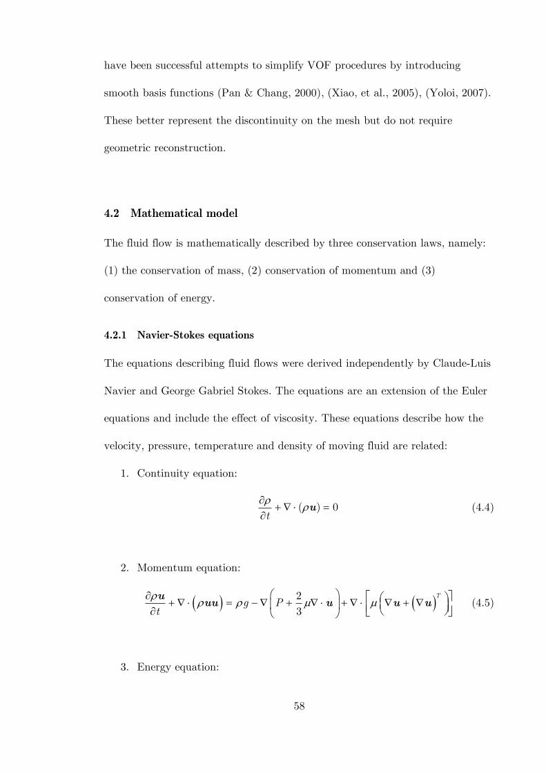
1. Continuity equation:
( ) 0t
u (4.4)
2. Momentum equation:
2
3
Tg P
t
uuu u u u (4.5)
3. Energy equation:
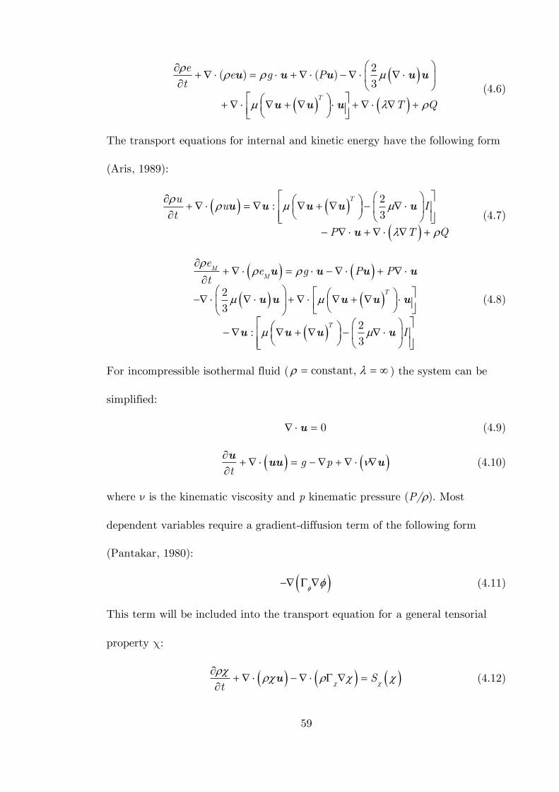
59
2( ) ( )
3
T
ee g P
t
T Q
u u u u u
u u u
(4.6)
The transport equations for internal and kinetic energy have the following form
(Aris, 1989):
2:
3
Tuu I
t
P T Q
u u u u u
u
(4.7)
2
3
2 :
3
MM
T
T
ee g P P
t
I
u u u u
u u u u u
u u u u
(4.8)
For incompressible isothermal fluid ( constant, ) the system can be
simplified:
0 u (4.9)
g pt
uuu u (4.10)
where is the kinematic viscosity and p kinematic pressure (P/). Most
dependent variables require a gradient-diffusion term of the following form
(Pantakar, 1980):
(4.11)
This term will be included into the transport equation for a general tensorial
property :
St
u (4.12)
60
4.2.2 Turbulence modelling
Turbulence is one of the most challenging problems in fluid dynamics.
The distinction between laminar, transitional and turbulent flow is not
unambiguous. Sometimes the flow appears in different states depending on the
location of the area of interest. The simplest way around this problem is to
calculate the flow as turbulent. The turbulent nature of the flow plays a crucial
part in the determination of relevant engineering parameters.
The most straightforward approach to the solution of turbulence is Direct
Numerical Simulation (DNS), which directly solves the Navier-Stokes equations.
Despite the performance of modern supercomputers a direct simulation of
turbulence by the time-dependent Navier-Stokes equation is applicable only to
relatively simple flow problems. To calculate the flow in other more realistic
cases, the complexity of the problem has to be reduced. This reduction is
carried out by applying an averaging operation to the Navier-Stokes equations.
The classical averaging method is the ensemble average, which produces the
Reynolds Averaged Navier-Stokes equations (RANS).
The most commonly used turbulence model in environmental CFD is the
standard k-ε model, since it has proven to be quite stable and often produces
reasonably realistic results. Many researchers have shown that the standard k-ε
turbulence model often produces a high turbulent viscosity and is not able to
capture the proper behaviour of turbulent boundary layers up to separation
61
(Bates, et al., 2005) (ERCOFTAC, 2000). The weaknesses of the standard k-ε
model can be summarized as follows:
Laminar and transitional regimes of flow cannot be modelled with the
standard k-ε model;
Regions of recirculation in a swirling flow are under-estimated;
The turbulent kinetic energy is over-predicted in regions of flow
impingement and reattachment leading to poor prediction of the
development of flow around leading edges;
Flow separation from surfaces under the action of adverse pressure
gradients is poorly predicted;
Flow recovery following re-attachment is poorly predicted;
Turbulence driven secondary flows in straight ducts of non-circular cross
section are not predicted at all.
Finally, considering the pros and cons of different methods, the k-ω turbulence
model was chosen for the turbulence modelling. This solves one equation for
turbulent kinetic energy and a second equation for the specific turbulent
dissipation rate (or turbulent frequency). The disadvantage of k-ω model is that
it requires fine mesh resolution near the wall. The advantages of k-ω turbulence
model are that it:
Allows for a more accurate near wall treatment;
Demonstrates superior performance for wall-bounded and low Reynolds
number flows;
Shows potential for predicting transition;
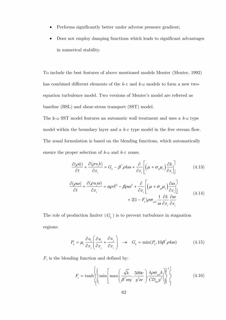
62
Performs significantly better under adverse pressure gradient;
Does not employ damping functions which leads to significant advantages
in numerical stability.
To include the best features of above mentioned models Menter (Menter, 1992)
has combined different elements of the k-ε and k-ω models to form a new two-
equation turbulence model. Two versions of Menter’s model are referred as
baseline (BSL) and shear-stress transport (SST) model.
The k-ω SST model features an automatic wall treatment and uses a k-ω type
model within the boundary layer and a k-ε type model in the free stream flow.
The zonal formulation is based on the blending functions, which automatically
ensure the proper selection of k-ω and k-ε zones.
*( )( ) ik k t
i i i
u kk kG k
t x x x
(4.13)
2 2
1 2
( )( )
1 2(1 )
it
i i i
i i
uS
t x x x
kF
x x
(4.14)
The role of production limiter (kG ) is to prevent turbulence in stagnation
regions:
* min( ,10 )ji ik t k k
j j i
uu uP G P k
x x x
(4.15)
F1 is the blending function and defined by:
4
21 * 2 2
4500tanh min max , ,
k
kkF
y y CD y
(4.16)
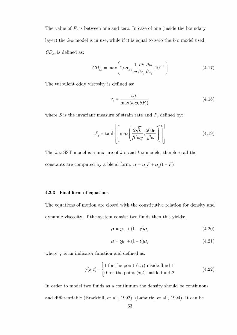
63
The value of F1 is between one and zero. In case of one (inside the boundary
layer) the k-ω model is in use, while if it is equal to zero the k-ε model used.
CDkω is defined as:
102
1max 2 ,10
ki i
kCD
x x
(4.17)
The turbulent eddy viscosity is defined as:
1
1 2max( , )t
a k
a SF
(4.18)
where S is the invariant measure of strain rate and F2 defined by:
2
2 * 2
2 500tanh max ,
kF
y y
(4.19)
The k-ω SST model is a mixture of k-ε and k-ω models; therefore all the
constants are computed by a blend form: 1 2
(1 )F F
4.2.3 Final form of equations
The equations of motion are closed with the constitutive relation for density and
dynamic viscosity. If the system consist two fluids then this yields:
1 2
(1 ) (4.20)
1 2
(1 ) (4.21)
where γ is an indicator function and defined as:
1 for the point ( , ) inside fluid 1
( , )0 for the point ( , ) inside fluid 2
x tx t
x t
(4.22)
In order to model two fluids as a continuum the density should be continuous
and differentiable (Brackbill, et al., 1992), (Lafaurie, et al., 1994). It can be
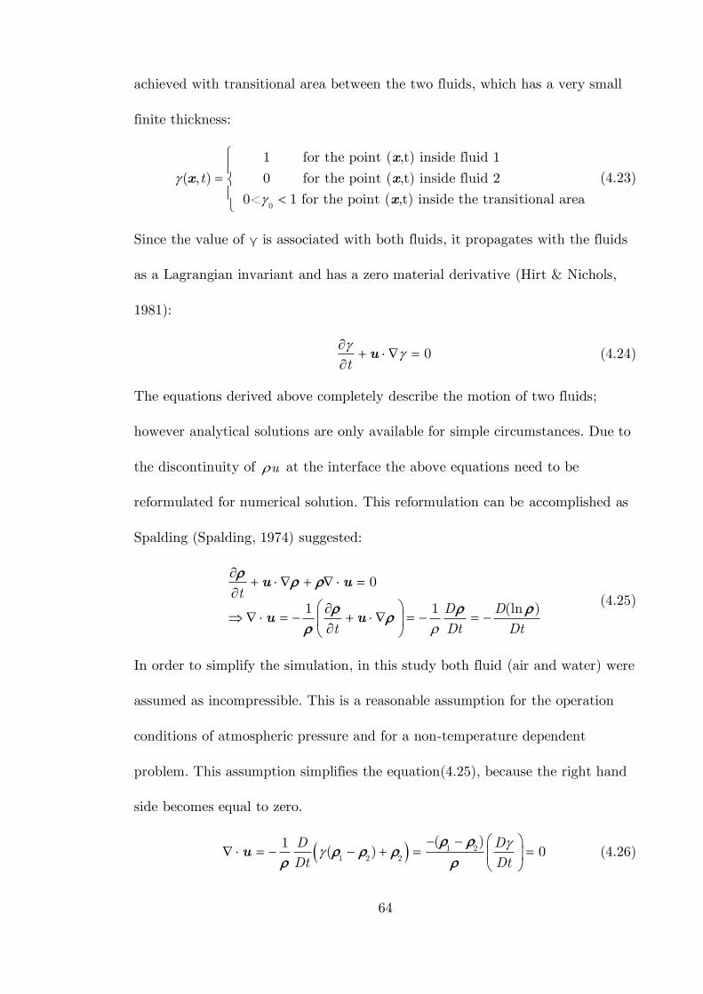
64
achieved with transitional area between the two fluids, which has a very small
finite thickness:
0
1 for the point ( ,t) inside fluid 1
( , ) 0 for the point ( ,t) inside fluid 2
0< 1 for the point ( ,t) inside the transitional area
t
x
x x
x
(4.23)
Since the value of γ is associated with both fluids, it propagates with the fluids
as a Lagrangian invariant and has a zero material derivative (Hirt & Nichols,
1981):
0t
u (4.24)
The equations derived above completely describe the motion of two fluids;
however analytical solutions are only available for simple circumstances. Due to
the discontinuity of u at the interface the above equations need to be
reformulated for numerical solution. This reformulation can be accomplished as
Spalding (Spalding, 1974) suggested:
0
1 1 (ln )t
D D
t Dt Dt
u u
u u
(4.25)
In order to simplify the simulation, in this study both fluid (air and water) were
assumed as incompressible. This is a reasonable assumption for the operation
conditions of atmospheric pressure and for a non-temperature dependent
problem. This assumption simplifies the equation(4.25), because the right hand
side becomes equal to zero.
1 21 2 2
( )1( ) 0
D D
Dt Dt
u
(4.26)
65
It is better to rearrange the transport equation for finite volume discretization
using the identity u u u and the incompressibility condition:
0t
u (4.27)
The momentum equation can also be simplified using the incompressibility
condition:
P g ft
u
u u u u
(4.28)
where fis the surface tension source term.
The final form continuity equation for incompressible flow, momentum equation
and α transport equation need to be solved simultaneously together with the
constitutive relations for density and dynamic viscosity.
4.2.4 Initial and boundary conditions
Regardless of the numerical methodology chosen to solve the governing
equations, suitable initial and boundary conditions have to be specified. The
initial conditions determine the state of fluid at time t=0, or at first step of an
iterative scheme.
Since the governing equations are a mixture of elliptic, parabolic and hyperbolic
behaviour, boundary conditions must be specified at each point of the closed
solution domain. Boundary conditions (BC) can be divided into two types:
Dirichlet BCs prescribe the value of the dependent variable on the
boundary and are therefore termed “fixed value”;
von Neumann BCs prescribe the gradient of the variable normal to the
boundary and are therefore termed “fixed gradient”
66
The most common physical boundary conditions in the discretised equation of
the finite volume are (Versteeg & Malalasekera, 2007):
Inlet boundary: The most common method is to fix the inlet velocity. Another
option is to specify the upstream stagnation pressure and velocity magnitude.
For this study, just like all multiphase flow modelling, this implies that the inlet
condition of the indicator function needs to be fixed.
Outlet boundary: It is vital that the outlet boundary condition is always
selected on the basis it has a weak influence on the upstream flow. It should be
placed as far away as possible from the region of interest and should be avoided
in regions of strong geometrical changes. The most common physical condition
for internal flows is to fix the downstream static pressure and zero gradient
condition is applied to the velocities. Another commonly used approach is when
the first row of cells next to the boundary is used to construct the velocity
distribution. The boundary velocities are then scaled according to this velocity
profile. If the boundary is placed where variation in the flow is small, then a
zero gradient condition to the indicator function can be applied.
Solid wall boundary: The normal velocity is zero; therefore no mass or other
convective flux can penetrate the solid body. The other variables at the wall,
the tangential velocity and pressure have to be determined by extrapolation
from the interior boundary.
Symmetry plane boundary: The surface normal gradients of all scalar fields are
zero at the symmetry plane, thus the convection flux through the symmetry is
67
zero as well. Viscous stress of velocity component parallel to the boundary is
zero.
The correct implementation of boundary condition is crucial point of every flow
solver. The accuracy of the solution is strongly depends on a proper physical
and numerical treatment of boundaries (Blazek, 2001). Furthermore the
robustness and convergence speed are considerably influenced.
4.3 Numerical Model
4.3.1 Introduction
This Section describes the procedure by which the equations presented in
Section 4.1 are solved numerically. The discretization used in the present study
is the well established finite volume method (Versteeg & Malalasekera, 2007),
(Blazek, 2001), (Hirsch, 2007). Finite volume method became popular in CFD
as a result of two advantages:
1. it ensures that the discretization is conservative (mass, momentum and
energy are conserved in a discrete sense);
2. it does not require coordinate transformation in order to be applied on
irregular meshes.
While the first property usually can be obtained using the finite difference
formulation, it is obtained naturally from the finite volume method. The second
property means that the finite volume method can be applied on unstructured
mesh consisting of arbitrary polyhedral. This increased flexibility is a great
advantage in generating a mesh for arbitrary geometries.
68
The finite volume method subdivides the flow domain into small control
volumes. The transport equations are integrated over the control volumes by
approximating the variation of flow properties between mesh points with
piecewise profiles. These piecewise approximations – or differencing schemes –
are constructed to support physical flow behaviour such as convection or
diffusion.
The solution procedure can be divided into three parts:
1. Discretization of solution domain into control volumes;
2. Numerical solution procedure;
3. Post processing where the results of the simulation are checked and
contour, vector plots prepared.
4.3.2 Full 3D model
4.3.2.1 Spatial discretization
The main advantage of the finite volume method is that the spatial
discretization is carried out directly in the physical space. In other words, there
are no problems with any transformation between coordinate systems, as in the
case of finite difference method (Blazek, 2001). There are several possibilities of
defining the shape and position of the control volume. Two basic approaches
can be distinguished: cell-centred scheme and cell-vertex scheme. The cell-
centred scheme, when the flow quantities are stored at the centroids of the
control volumes. In case of cell-vertex scheme the flow variables are stored at
the mesh points. The approach used in this study the so called co-located
variable arrangement (Peric, 1985) where all the flow properties are defined at
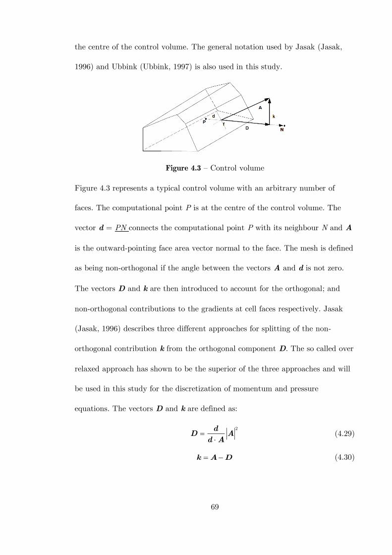
69
the centre of the control volume. The general notation used by Jasak (Jasak,
1996) and Ubbink (Ubbink, 1997) is also used in this study.
Figure 4.3 – Control volume
Figure 4.3 represents a typical control volume with an arbitrary number of
faces. The computational point P is at the centre of the control volume. The
vector d = PN connects the computational point P with its neighbour N and A
is the outward-pointing face area vector normal to the face. The mesh is defined
as being non-orthogonal if the angle between the vectors A and d is not zero.
The vectors D and k are then introduced to account for the orthogonal; and
non-orthogonal contributions to the gradients at cell faces respectively. Jasak
(Jasak, 1996) describes three different approaches for splitting of the non-
orthogonal contribution k from the orthogonal component D. The so called over
relaxed approach has shown to be the superior of the three approaches and will
be used in this study for the discretization of momentum and pressure
equations. The vectors D and k are defined as:
2
dD A
d A (4.29)
k A D (4.30)
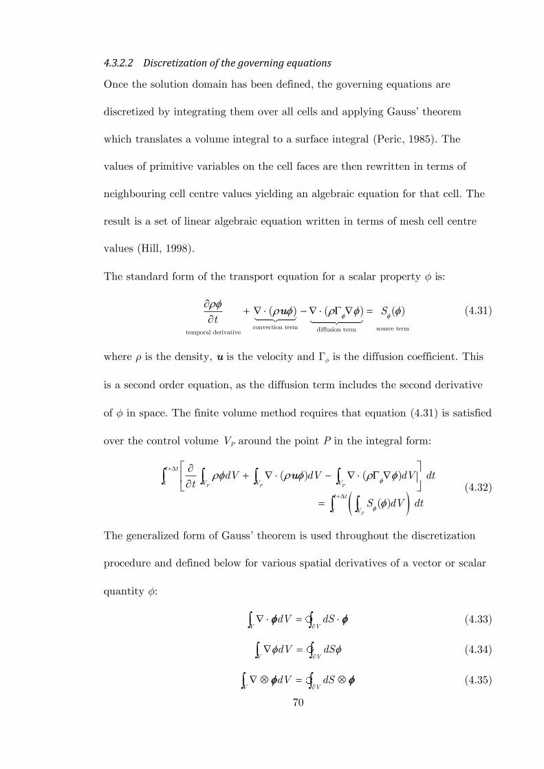
70
4.3.2.2 Discretization of the governing equations
Once the solution domain has been defined, the governing equations are
discretized by integrating them over all cells and applying Gauss’ theorem
which translates a volume integral to a surface integral (Peric, 1985). The
values of primitive variables on the cell faces are then rewritten in terms of
neighbouring cell centre values yielding an algebraic equation for that cell. The
result is a set of linear algebraic equation written in terms of mesh cell centre
values (Hill, 1998).
The standard form of the transport equation for a scalar property is:
convection term source termdiffusion termtemporal derivative
( ) ( ) ( )St
u (4.31)
where is the density, u is the velocity and is the diffusion coefficient. This
is a second order equation, as the diffusion term includes the second derivative
of in space. The finite volume method requires that equation (4.31) is satisfied
over the control volume VP around the point P in the integral form:
( ) ( )
( )
P P P
P
t t
t V V V
t t
t V
dV dV dV dtt
S dV dt
u (4.32)
The generalized form of Gauss’ theorem is used throughout the discretization
procedure and defined below for various spatial derivatives of a vector or scalar
quantity :
V V
dV dS
(4.33)
V VdV dS
(4.34)
V V
dV dS
(4.35)
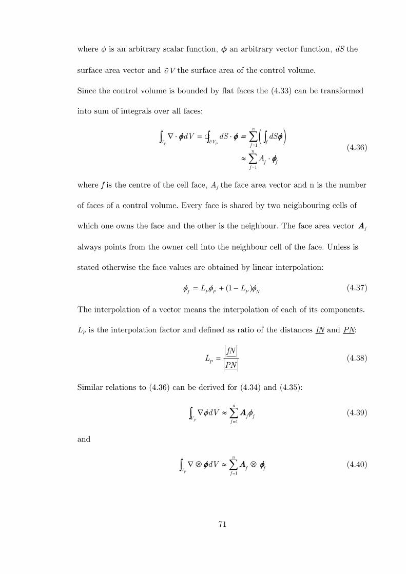
71
where is an arbitrary scalar function, an arbitrary vector function, dS the
surface area vector and V the surface area of the control volume.
Since the control volume is bounded by flat faces the (4.33) can be transformed
into sum of integrals over all faces:
1
1
P P
n
V V ffn
f ff
dV dS dS
A
(4.36)
where f is the centre of the cell face, Af the face area vector and n is the number
of faces of a control volume. Every face is shared by two neighbouring cells of
which one owns the face and the other is the neighbour. The face area vector Af
always points from the owner cell into the neighbour cell of the face. Unless is
stated otherwise the face values are obtained by linear interpolation:
(1 )f P P P NL L (4.37)
The interpolation of a vector means the interpolation of each of its components.
LP is the interpolation factor and defined as ratio of the distances fN and PN:
P
fNL
PN (4.38)
Similar relations to (4.36) can be derived for (4.34) and (4.35):
1P
n
f fVf
dV
A (4.39)
and
1
P
n
f fVf
dV
A (4.40)
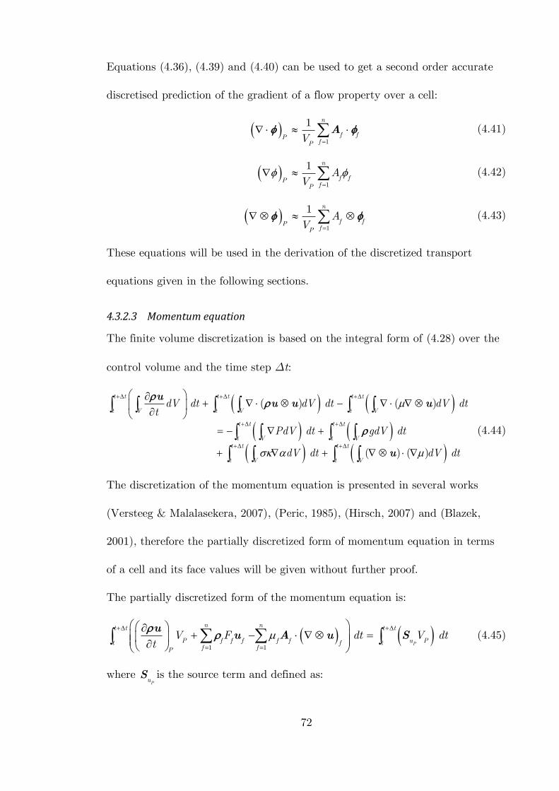
72
Equations (4.36), (4.39) and (4.40) can be used to get a second order accurate
discretised prediction of the gradient of a flow property over a cell:
1
1 n
f fPfP
V
A (4.41)
1
1 n
f fPfP
AV
(4.42)
1
1 n
f fPfP
AV
(4.43)
These equations will be used in the derivation of the discretized transport
equations given in the following sections.
4.3.2.3 Momentum equation
The finite volume discretization is based on the integral form of (4.28) over the
control volume and the time step t:
( ) ( )
( ) ( )
t t t t t t
t V t V t V
t t t t
t V t Vt t t t
t V t V
dV dt dV dt dV dtt
PdV dt gdV dt
dV dt dV
uu u u
u
dt
(4.44)
The discretization of the momentum equation is presented in several works
(Versteeg & Malalasekera, 2007), (Peric, 1985), (Hirsch, 2007) and (Blazek,
2001), therefore the partially discretized form of momentum equation in terms
of a cell and its face values will be given without further proof.
The partially discretized form of the momentum equation is:
1 1
P
n nt t t t
P f f f f f u Pt tff fP
V F dt V dtt
uu A u S
(4.45)
where PuS is the source term and defined as:
73
Pu P PP P P P
P g S u (4.46)
The terms of interest in the above equation are the convection, diffusion and
curvature terms. These terms are discussed in the following sections. The
gradients over a cell of different flow properties can be calculated according to
equations (4.42) and (4.43).
4.3.2.3.1 Convection term
The finite volume discretization of the convection term yields:
( ) ( )
( )
Pf fV
f
f f ff
f ff
dV
u A u
A u
F
(4.47)
where Ff is the face mass flux through the face:
( )f f f
F A u (4.48)
The cell face flux is calculated by the solution algorithm. The cell face average
value (f) is determined from the cell nodal values via the differencing scheme.
Jasak (Jasak, 1996) analysed a number of differencing schemes in terms of
boundedness, stability, accuracy and required computational resource.
Considering the advantage and disadvantage of different differencing schemes
the upwind (Pantakar, 1980) and Gamma (Jasak, 1996) schemes have been
chosen for this study. The Gamma scheme guaranties a bounded solution whilst
minimising the numerical diffusion of sharp changes in gradient of the variable.
The upwind scheme determines the value of at the cell face by considering the
direction of flow is normal to the cell face. The value at the cell face is equal to
the value of the cell node from the upwind direction:
74
max ,0 max ,0f f P N F F F (4.49)
where the subscript P and N indicates the current and neighbouring cell values.
The Gamma scheme is a high resolution second order convection-diffusion
differencing scheme based on the Normalised Variable Diagram (NVD)
(Leonard, 1991), specially developed for unstructured meshes. The magnitude
(u) of the velocity vector (u) is defined as:
for 0 or 1
1( ) for 1
2
1 for 02 2
D D D
f D A D
D DD A D
u u u
u u u k u
u uu u u k
k k
(4.50)
where k is prescribed constant with a value between 0 and 0.5. The
recommended value is 0.1. The subscripts D and A are determined by the
direction of flow:
0 & or 0 &f fF D P A N F D N A P (4.51)
The decision factor Du is defined as:
12( )A D
DD
u uu
u
d (4.52)
and calculated according to (4.42):
1
1( )
n
D f ffD
u uV
A (4.53)
4.3.2.3.2 Diffusion term
The diffusion term will be discretised in a similar way. Using the assumption of
linear variation of :
75
1
( ) ( )P
n
f f fVf
dV
u A u (4.54)
where the dynamic viscosity at the face (f) is calculated by linear interpolation
with LP calculated from (4.38):
(1 )f P P P NL L (4.55)
For an orthogonal mesh, the calculation of the gradient at the cell face is
relatively straightforward using the nodal values straddling the cell face.
Considering (4.29) and Af=Df then it is possible for an orthogonal mesh to use
the following expression for the dot product between the face area vector and
the velocity gradient at the face:
( ) ( ) N Pf f f f f
f
u uA u D u D
d (4.56)
If the mesh is non-orthogonal it is necessary to introduce an additional term to
compensate the non-orthogonal contribution. This is done by Af=Df+kf, the
over relaxed non orthogonal decomposition of the face area vector (Jasak, 1996),
(Ubbink, 1997):
orthogonal contribution non-orthogonal correction
( ) ( ) ( )f f f f f f A u D u k u (4.57)
In this case the orthogonal correction is treated explicitly.
4.3.2.3.3 Source term
Terms of the general transport equation which cannot be treated as convective
or diffusive term are included in the source term. The source term S(), can be
a general function of . The treatment of these terms follows the work of
76
Pantakar (Pantakar, 1980), in which the source terms are linearized before the
actual discretization:
( )S Su Sp (4.58)
where Su and Sp can also depend on . Integration of (4.58) over the control
volume yields:
( )P
P P PVS dV SuV SpV (4.59)
Su is directly added to any existing source term. If Sp is negative, then it can be
added to the central coefficient of the solution matrix increasing its diagonal
dominance and enhancing the stability of the solution (Brennan, 2001). If it is
positive then it is solved explicitly.
4.3.2.4 Temporal discretization
Early applications of CFD were mostly focused on steady state solutions. These
have a benefit of being easier to solve in terms of complexity and computer
requirements. Nowadays the attention is being focused on unsteady simulation.
In these cases, in addition to the question of spatial discretization, there is the
question of temporal discretization.
In the previous Section we have described the discretization of the volume
integrals in the standard transport equation in integral form:
( ) ( )
( )
P P P
P
t t
t V V V
t t
t V
dV dV dV dtt
S dV dt
u (4.32)
Assuming that the control volume does not change in time, the equation (4.32)
can be written as:
77
( ) ( )
( )
t t
P f f f ftf fP
t t
P P Pt
V F dtt
SuV SpV dt
A (4.60)
This expression is usually referred to as a “semi-discretized” form of the
transport equation (Hirsch, 2007). The temporal integrals and time derivative
can be calculated directly as:
n n o oP P P P
Pt t
(4.61)
1
( ) ( )2
t t o n
tt dt t
(4.62)
where
( )
( )
n
o
t t
t
(4.63)
Assuming that the density and diffusivity do not change in time, equations
(4.60), (4.61) and (4.62) give:
1 1( ) ( )
2 21 1
( ) ( )2 2
1 1
2 2
n on nP P P P
P f f f ff f
o of f f f
f f
n oP P P P P
V Ft
F
SuV SpV SpV
A
A (4.64)
Since f
and ( )f
also depends on values of in the surrounding cells (4.64)
produces an algebraic equation:
n nP P N N
N
a a Su (4.65)
where the subscript N denotes the nearest neighbours.
It is useful to present the discretised momentum equation as:
78
( ) 1
( )P P
n PP P
P P
Pa a
H u
u (4.66)
where PP Pa a and:
( ) nP N N P
N
a Su H u u (4.67)
This formulation of the discretized momentum equation will be used for the
derivation of the pressure equation.
4.3.2.5 Pressure equation
The pressure equation is derived from the incompressibility condition and the
discretized momentum equation. The discretized continuity equation has the
following form:
0f fV
f
dV u A u (4.68)
The discretized momentum equation (4.66) is used to predict the face value of
the velocity. This is done by isolating the contribution of the pressure from
(4.66) when interpolating it to the face. The contribution of the pressure
gradient at the face is then added explicitly to uf by calculating it directly from
the pressure values at the nodes sharing the face. The face value of velocity is:
( ) 1
( )f f
P Pf
Pa a
H uu (4.69)
The face values other than pressure gradient are calculated by using linear
interpolation:
( ) ( ) ( )
(1 )P P
P P Pf P N
L La a a
H u H u H u (4.70)
1 1 1
(1 )P P
P P Pf P N
L La a a
(4.71)
79
Substitution of uf from (4.69) into (4.68) gives:
1 ( )
( )f f f
f fP Pf f
Pa a
H uA A (4.72)
Taking into account the orthogonal and non-orthogonal contribution of
neighbours, the pressure gradient over the faces can be calculated similarly to
diffusion term. Using the over relaxed non-orthogonal decomposition of the face
area vector:
orthogonal contribution non-orthogonal correction
( ) ( ) ( )f f f f f f
P P P A D k (4.73)
The orthogonal contribution is given by:
( ) N Pf f f
f
P PP
D D
d (4.74)
and the non orthogonal correction is:
1 1
( ) (1 )f f f P f f P f f
f fP Nf N
P L P L PV V
k k A A (4.75)
The non-orthogonal correction is treated explicitly by adding it to the source
term:
1
( )f f
f P f
P Spa
D (4.76)
where
( ) 1
( )f f f
f fP Pf f
Sp Pa a
H uA k (4.77)
Now it is possible to reformulate the pressure equation:
P P N N
N
a P a P Sp (4.78)
80
4.3.2.6 Solution algorithm
The fluid in this study assumed to be Newtonian and incompressible. It follows
there is no explicit equation for pressure, therefore special care needs to be
taken to avoid de-coupling of pressure from velocity. It can be done by deriving
the discretized pressure equation from a semi-discretized momentum equation,
using the continuity restriction of a divergence free velocity field. The solution
procedure applied in this study is based on PISO algorithm.
4.3.2.6.1 Pressure-velocity coupling with PISO
Pressure Implicit with Splitting of Operators (PISO) algorithm is a pressure-
velocity treatment for transient flow calculation proposed by Issa (Issa, 1986).
PISO is a segregated approach for solving the Navier-Stokes equations, where
pressure and velocity are treated sequentially using the predictor-corrector
procedure. The summary of the algorithm is presented by Jasak (Jasak, 1996)
and Rusche (Rusche, 2002).
The pressure-velocity coupling is applied in three main steps:
1. Momentum predictor step: the pressure is used to solve the momentum
equation and obtain the first approximation of velocity. The first
approximation of velocity is not satisfies the continuity restriction.
2. Pressure solution step: the matrix of pressure equation is assembled and
solved to get the new estimation for the pressure.
3. Explicit velocity correction step: the pressure obtained in previous step is
used to calculate the conservative volumetric fluxes and reconstruct the
velocities which are consistent with the pressure field.
81
The velocity depends on the pressure field and the contribution from the
updated velocities of neighbouring cells. Therefore the last two steps are
repeated until the predefined tolerance condition is satisfied. When the PISO
loop is finished the velocity is corrected with the correct pressure gradient.
4.3.2.6.2 Solution of linear equation systems
The discretization procedure converts every partial differential into a system of
linear algebraic equation. Each governing equation has its own unique linear
equation system; however they all have the same general form:
n nP P N N
N
a a b (4.79)
in matrix notation:
A b (4.80)
The diagonal elements of matrix A contain aP, while the off diagonal elements
of A contain aN. Φ is the array of unknown and b is the source array.
Equation (4.80) is solved with an iterative procedure. This procedure starts with
an initial guess and improves the solution in every iteration until satisfy the
prescribed condition, which is the difference between two consecutive solution.
The convergence rate can be improved by applying preconditioning matrix. In
this study, for symmetric matrixes the Preconditioned Conjugate Gradient
(PCG) solver with Diagonal-based Incomplete Cholesky (DIC) preconditioner
was used. For asymmetric matrixes the Preconditioned Bi-Conjugate Gradient
(PBiCG) with Diagonal-based Incomplete Lower-Upper (DILU) preconditioner
was applied.
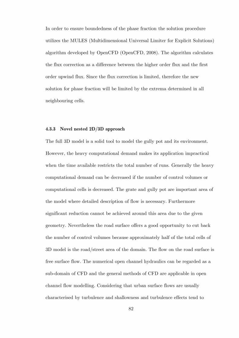
82
In order to ensure boundedness of the phase fraction the solution procedure
utilizes the MULES (Multidimensional Universal Limiter for Explicit Solutions)
algorithm developed by OpenCFD (OpenCFD, 2008). The algorithm calculates
the flux correction as a difference between the higher order flux and the first
order upwind flux. Since the flux correction is limited, therefore the new
solution for phase fraction will be limited by the extrema determined in all
neighbouring cells.
4.3.3 Novel nested 2D/3D approach
The full 3D model is a solid tool to model the gully pot and its environment.
However, the heavy computational demand makes its application impractical
when the time available restricts the total number of runs. Generally the heavy
computational demand can be decreased if the number of control volumes or
computational cells is decreased. The grate and gully pot are important area of
the model where detailed description of flow is necessary. Furthermore
significant reduction cannot be achieved around this area due to the given
geometry. Nevertheless the road surface offers a good opportunity to cut back
the number of control volumes because approximately half of the total cells of
3D model is the road/street area of the domain. The flow on the road surface is
free surface flow. The numerical open channel hydraulics can be regarded as a
sub-domain of CFD and the general methods of CFD are applicable in open
channel flow modelling. Considering that urban surface flows are usually
characterised by turbulence and shallowness and turbulence effects tend to
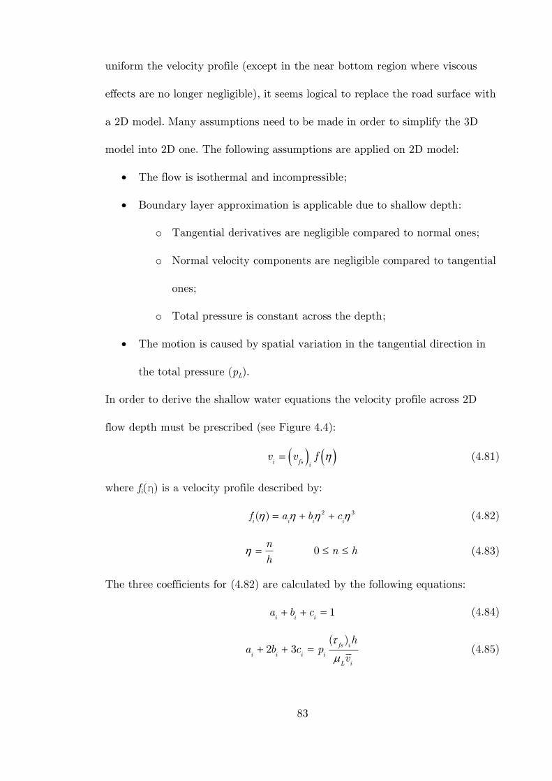
83
uniform the velocity profile (except in the near bottom region where viscous
effects are no longer negligible), it seems logical to replace the road surface with
a 2D model. Many assumptions need to be made in order to simplify the 3D
model into 2D one. The following assumptions are applied on 2D model:
The flow is isothermal and incompressible;
Boundary layer approximation is applicable due to shallow depth:
o Tangential derivatives are negligible compared to normal ones;
o Normal velocity components are negligible compared to tangential
ones;
o Total pressure is constant across the depth;
The motion is caused by spatial variation in the tangential direction in
the total pressure (pL).
In order to derive the shallow water equations the velocity profile across 2D
flow depth must be prescribed (see Figure 4.4):
i fs iv v f (4.81)
where fi(η) is a velocity profile described by:
2 3( )i i i if a b c (4.82)
0n
n hh
(4.83)
The three coefficients for (4.82) are calculated by the following equations:
1i i ia b c (4.84)
( )
2 3 fs i
i i i iL i
ha b c p
v
(4.85)
84
2
2 ii s L L ti i
L i
p hb p g
v
(4.86)
Figure 4.4 – Velocity calculation on 2D domain
4.3.3.1 Spatial discretization
Discretization of the spatial domain results in a two-dimensional computational
grid, which consists of a finite number of non-overlapping control surfaces.
Figure 4.5 – Control surface
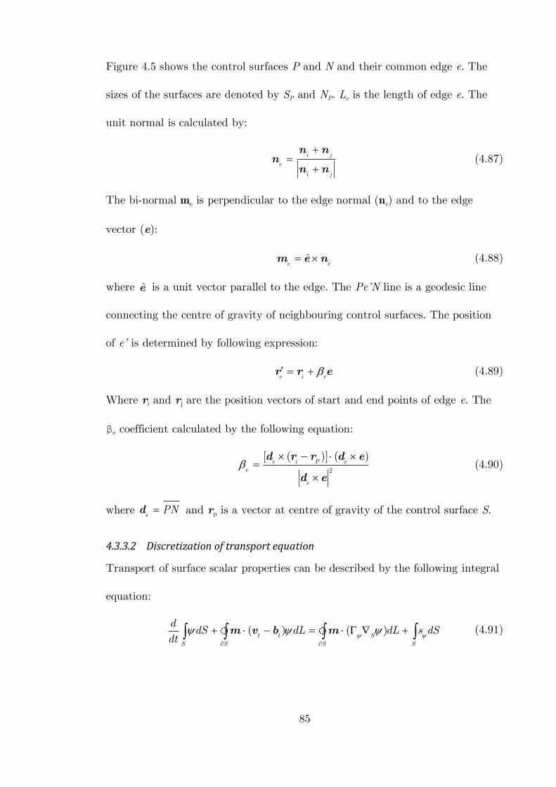
85
Figure 4.5 shows the control surfaces P and N and their common edge e. The
sizes of the surfaces are denoted by SP and NP. Le is the length of edge e. The
unit normal is calculated by:
i j
e
i j
n nn
n n (4.87)
The bi-normal me is perpendicular to the edge normal (ne) and to the edge
vector (e):
ˆe e m e n (4.88)
where e is a unit vector parallel to the edge. The Pe’N line is a geodesic line
connecting the centre of gravity of neighbouring control surfaces. The position
of e’ is determined by following expression:
e i e
r r e (4.89)
Where ri and rj are the position vectors of start and end points of edge e. The
βe coefficient calculated by the following equation:
2
[ ( )] ( )e i P e
e
e
d r r d e
d e (4.90)
where ePNd and rp is a vector at centre of gravity of the control surface S.
4.3.3.2 Discretization of transport equation
Transport of surface scalar properties can be described by the following integral
equation:
( ) ( )t t S
S S S S
ddS dL dL s dS
dt
m v b m (4.91)
86
Similarly to the volume 3D method, the transport equation must be satisfied for
each control surface element. Accordingly, the spatial integrals in equation
(4.91) should be integrated in the control surface SP.
( )P P P P
t SS S S S
ddS dL dL s dS
dt
m v m (4.92)
Spatial discretization of (4.92) was carried out assuming linear distribution of
the variables on the control surface P:
( ) ( ) ( )P P S P
r r r (4.93)
Assuming linear distribution of ψ in time and space is sufficient to achieve a
second order accuracy of the discretization method.
4.3.3.3 Discretization of spatial integrals
Taking into account that the control area is limited by straight edges, the line
integral over the boundary of control surface can be written as the sum of edges
line integrals:
( ) ( )P e
eS L
dL dL r r (4.94)
Applying the rules of central point:
( )e
e eL
dL L r (4.95)
where ( )e e
r
4.3.3.3.1 Convection term
Discretization of convective term is carried out using (4.94) and (4.95):
87
( )
P
t e t e e eeS
e ee
dL L
s
m v m v (4.96)
where ( )e e t e es Lm v
The value of ψ on edge e is calculated from the values of the centre points of
adjacent control surface. Using central discretization scheme the value of ψ on
the edge is calculated as follows:
(1 )e x P x Ne e (4.97)
where the interpolation factor ex defined as the ratio of eN and PN :
x
eNe
PN (4.98)
4.3.3.3.2 Diffusion term
Using (4.94) and (4.95) the discretised diffusion term can be expressed as
follows:
( ) ( )
= ( ) ( )
S e S e eeS
e e e S ee
dL L
L
m m
m (4.99)
where ( )e S e
m is a normal surface gradient of ψ on edge e.
Discretization of the surface normal gradient depends on the othogonality of the
grid. In this study an orthogonal grid has been used for the 2D domain;
therefore there is no need to go into the details of the non-orthogonality issue.
In the case of an orthogonal grid the normal surface gradient of ψ on edge e is:
( ) N Pe S e
PNL
m (4.100)
and
88
1
( ) ( )S P P P e e e
eP
LS
I n n m (4.101)
where ψe is value of ψ on the edge of control surface from the previous iteration.
4.3.3.4 Temporal discretization
After spatial discretization the transport equation has the following form:
( ) ( ) ( )P P e e e e e s e u P p P P
e e
dS s L s S s S
dt m (4.102)
Using the implicit Gear method for time discretization a fully discretised
transport equation has the following form:
3 4
( ) ( )
n n o o oo ooP p P P P P n n
e ee
n n n n n n n n ne e e s e u P p P P
e
S S Ss
tL s S s S
m (4.103)
4.3.3.5 Solution of linear equation systems
Taking into account that , n ne e
m and ( )ns e do not depend on the value of ψ
at the centre of adjacent control surface at the time tn, similarly to 3D model
the linear equations has the following from:
n nP P N N P
N
a a r (4.104)
In case of combined convection discretization and the Gear time discretization
method the coefficients and the right side of the equation are defined by the
following expression:
3
1 max sgn ,02
( )
nn n n n nP
P e f e e xe
nen n n n
e e p Pne
e
Sa s s e
t
L s S
d
(4.105)
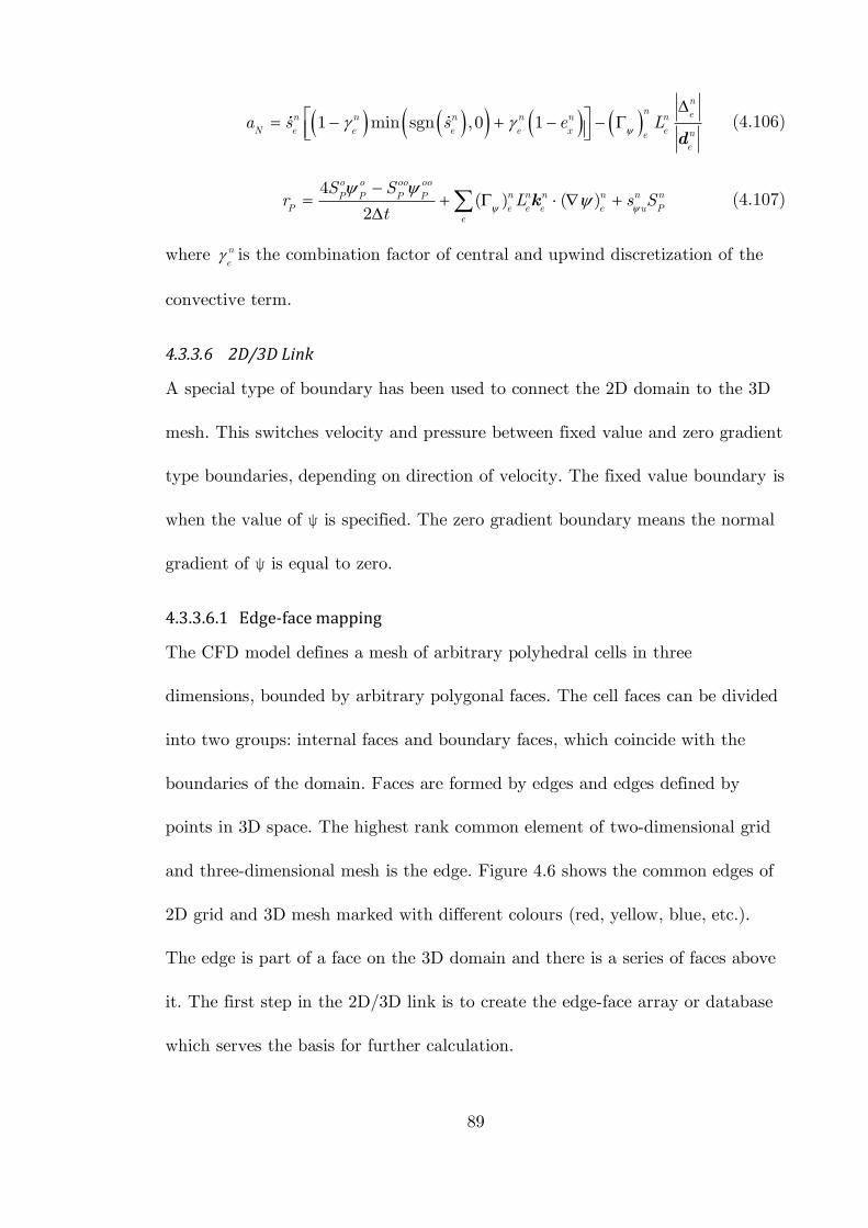
89
1 min sgn ,0 1
nn en n n n n n
N e e e e x e nee
a s s e L
d
(4.106)
4
( ) ( )2
o o oo oon n n n n nP P P P
P e e e e u Pe
S Sr L s S
t
k (4.107)
where ne is the combination factor of central and upwind discretization of the
convective term.
4.3.3.6 2D/3D Link
A special type of boundary has been used to connect the 2D domain to the 3D
mesh. This switches velocity and pressure between fixed value and zero gradient
type boundaries, depending on direction of velocity. The fixed value boundary is
when the value of ψ is specified. The zero gradient boundary means the normal
gradient of ψ is equal to zero.
4.3.3.6.1 Edge-face mapping
The CFD model defines a mesh of arbitrary polyhedral cells in three
dimensions, bounded by arbitrary polygonal faces. The cell faces can be divided
into two groups: internal faces and boundary faces, which coincide with the
boundaries of the domain. Faces are formed by edges and edges defined by
points in 3D space. The highest rank common element of two-dimensional grid
and three-dimensional mesh is the edge. Figure 4.6 shows the common edges of
2D grid and 3D mesh marked with different colours (red, yellow, blue, etc.).
The edge is part of a face on the 3D domain and there is a series of faces above
it. The first step in the 2D/3D link is to create the edge-face array or database
which serves the basis for further calculation.
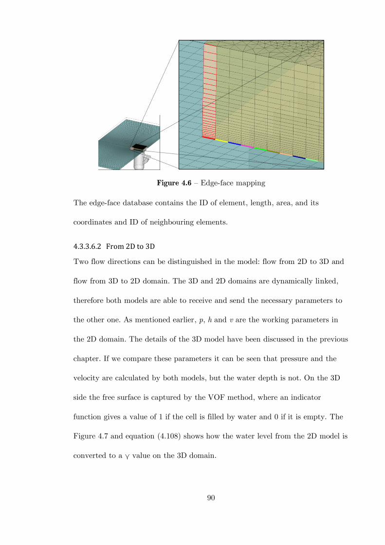
90
Figure 4.6 – Edge-face mapping
The edge-face database contains the ID of element, length, area, and its
coordinates and ID of neighbouring elements.
4.3.3.6.2 From 2D to 3D
Two flow directions can be distinguished in the model: flow from 2D to 3D and
flow from 3D to 2D domain. The 3D and 2D domains are dynamically linked,
therefore both models are able to receive and send the necessary parameters to
the other one. As mentioned earlier, p, h and v are the working parameters in
the 2D domain. The details of the 3D model have been discussed in the previous
chapter. If we compare these parameters it can be seen that pressure and the
velocity are calculated by both models, but the water depth is not. On the 3D
side the free surface is captured by the VOF method, where an indicator
function gives a value of 1 if the cell is filled by water and 0 if it is empty. The
Figure 4.7 and equation (4.108) shows how the water level from the 2D model is
converted to a γ value on the 3D domain.
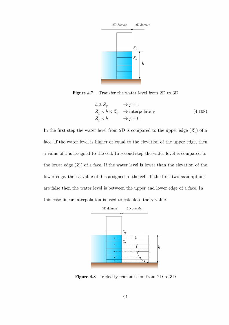
91
Figure 4.7 – Transfer the water level from 2D to 3D
1
interpolate
0
U
L U
L
h Z
Z h Z
Z h
(4.108)
In the first step the water level from 2D is compared to the upper edge (ZU) of a
face. If the water level is higher or equal to the elevation of the upper edge, then
a value of 1 is assigned to the cell. In second step the water level is compared to
the lower edge (ZL) of a face. If the water level is lower than the elevation of the
lower edge, then a value of 0 is assigned to the cell. If the first two assumptions
are false then the water level is between the upper and lower edge of a face. In
this case linear interpolation is used to calculate the γ value.
Figure 4.8 – Velocity transmission from 2D to 3D
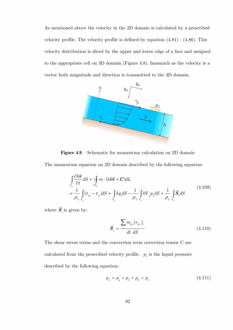
92
As mentioned above the velocity in the 2D domain is calculated by a prescribed
velocity profile. The velocity profile is defined by equation (4.81) - (4.86). This
velocity distribution is sliced by the upper and lower edge of a face and assigned
to the appropriate cell on 3D domain (Figure 4.8). Inasmuch as the velocity is a
vector both magnitude and direction is transmitted to the 3D domain.
Figure 4.9 – Schematic for momentum calculation on 2D domain
The momentum equation on 2D domain described by the following equation:
( )
1 1 1( )
w w
w w w w
S S
fs w t s L vS S S SL L L
hdS m h dLt
dS hg dS h p dS dS
vvv C
S (4.109)
where vS is given by:
, ,( )
d i d i ti
v
m v
dt dS
S (4.110)
The shear stress terms and the convection term correction tensor C are
calculated from the prescribed velocity profile. pL is the liquid pressure
described by the following equation:
L g d hp p p p p
(4.111)
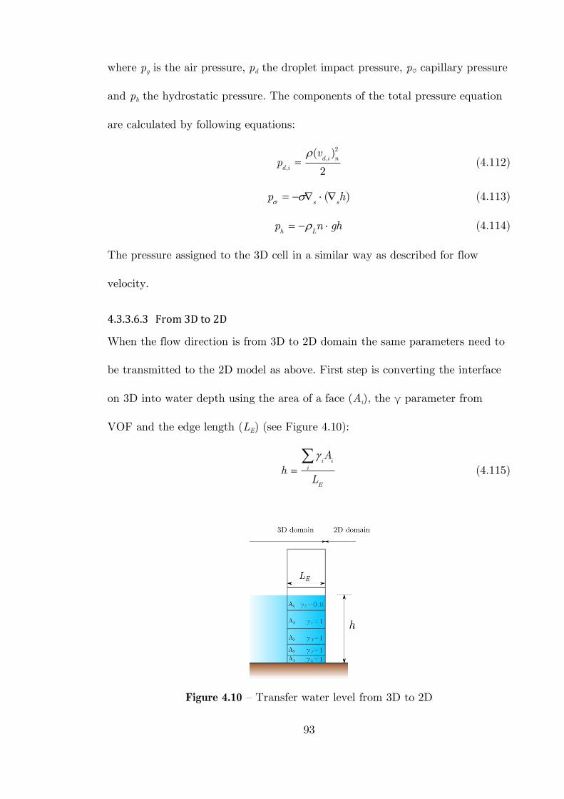
93
where pg is the air pressure, pd the droplet impact pressure, pσ capillary pressure
and ph the hydrostatic pressure. The components of the total pressure equation
are calculated by following equations:
2
,
,
( )
2d i n
d i
vp
(4.112)
( )s s
p h
(4.113)
h Lp n gh (4.114)
The pressure assigned to the 3D cell in a similar way as described for flow
velocity.
4.3.3.6.3 From 3D to 2D
When the flow direction is from 3D to 2D domain the same parameters need to
be transmitted to the 2D model as above. First step is converting the interface
on 3D into water depth using the area of a face (Ai), the γ parameter from
VOF and the edge length (LE) (see Figure 4.10):
i i
i
E
Ah
L
(4.115)
Figure 4.10 – Transfer water level from 3D to 2D
94
In the case of the velocity, the necessary parameters for equation (4.81) - (4.86)
are calculated by 3D model except v . The following equation is used to
calculate the average velocity:
0
1 hv vdhh
(4.116)
4.4 Mesh Creation
Once the problem has been specified an appropriate set of governing equations
and boundary conditions have been selected. Next step is dividing the flow
domain into cells. The design and construction of a quality mesh is crucial to
the success of CFD analysis. The mesh has a significant impact on the rate of
convergence, solution accuracy and CPU time required. Many different meshing
strategies exist, including structured, unstructured, hybrid, composite and
overlapping grids. The choices of numerical method and gridding strategy are
strongly interdependent.
Traditionally, grids have been divided into structured and unstructured grids.
The structured grids are built up from quadrilateral elements. Therefore the
structured grids have a well defined structure, from which the neighbours of a
particular volume can be readily deduced on the basis of the location of the
volume in the structure. Usually, a structured grid requires less memory and has
better numerical properties. However it is difficult to mesh complex geometries
using structured meshes.
The structured meshes have the following characteristics in common:
A simple data structure is used to describe the mesh;
95
All cells have a similar shape;
Cell faces and edges can be mapped to lie parallel to coordinate axes;
Mesh quality deteriorates with increasing complexity of the domain
One characteristic used to distinguish between structured and unstructured
meshes is the existence of an obvious mapping between logical space and
physical space for the mesh (Hansen, et al., 2005). Unstructured grids are built
from different elements, mainly from triangular ones. In case of unstructured
grids the volumes can be ordered arbitrarily. The connections between the
neighbours have to be defined explicitly.
The unstructured meshes have the following properties in common:
The data structures is more complex;
Cells have variable local topology and size;
Cell faces and edges do not have an implied orientation;
Mesh quality remains high as the domain complexity increase.
The meshing process can be divided into the following steps:
1. Geometry definition
2. Geometry decomposition
3. Mesh generation
4. Checking mesh quality, refining
5. Definition of boundary conditions
In the phase of defining the mesh we need to take into account whether the
solver is uses a cell centred or a node centred algorithm. A cell centred solver
creates control volumes that are completely identical to the grid. A node
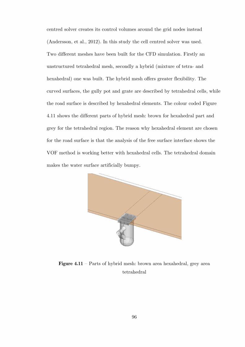
96
centred solver creates its control volumes around the grid nodes instead
(Andersson, et al., 2012). In this study the cell centred solver was used.
Two different meshes have been built for the CFD simulation. Firstly an
unstructured tetrahedral mesh, secondly a hybrid (mixture of tetra- and
hexahedral) one was built. The hybrid mesh offers greater flexibility. The
curved surfaces, the gully pot and grate are described by tetrahedral cells, while
the road surface is described by hexahedral elements. The colour coded Figure
4.11 shows the different parts of hybrid mesh: brown for hexahedral part and
grey for the tetrahedral region. The reason why hexahedral element are chosen
for the road surface is that the analysis of the free surface interface shows the
VOF method is working better with hexahedral cells. The tetrahedral domain
makes the water surface artificially bumpy.
Figure 4.11 – Parts of hybrid mesh: brown area hexahedral, grey area
tetrahedral
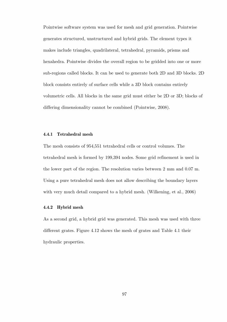
97
Pointwise software system was used for mesh and grid generation. Pointwise
generates structured, unstructured and hybrid grids. The element types it
makes include triangles, quadrilateral, tetrahedral, pyramids, prisms and
hexahedra. Pointwise divides the overall region to be gridded into one or more
sub-regions called blocks. It can be used to generate both 2D and 3D blocks. 2D
block consists entirely of surface cells while a 3D block contains entirely
volumetric cells. All blocks in the same grid must either be 2D or 3D; blocks of
differing dimensionality cannot be combined (Pointwise, 2008).
4.4.1 Tetrahedral mesh
The mesh consists of 954,551 tetrahedral cells or control volumes. The
tetrahedral mesh is formed by 199,394 nodes. Some grid refinement is used in
the lower part of the region. The resolution varies between 2 mm and 0.07 m.
Using a pure tetrahedral mesh does not allow describing the boundary layers
with very much detail compared to a hybrid mesh. (Wilkening, et al., 2006)
4.4.2 Hybrid mesh
As a second grid, a hybrid grid was generated. This mesh was used with three
different grates. Figure 4.12 shows the mesh of grates and Table 4.1 their
hydraulic properties.
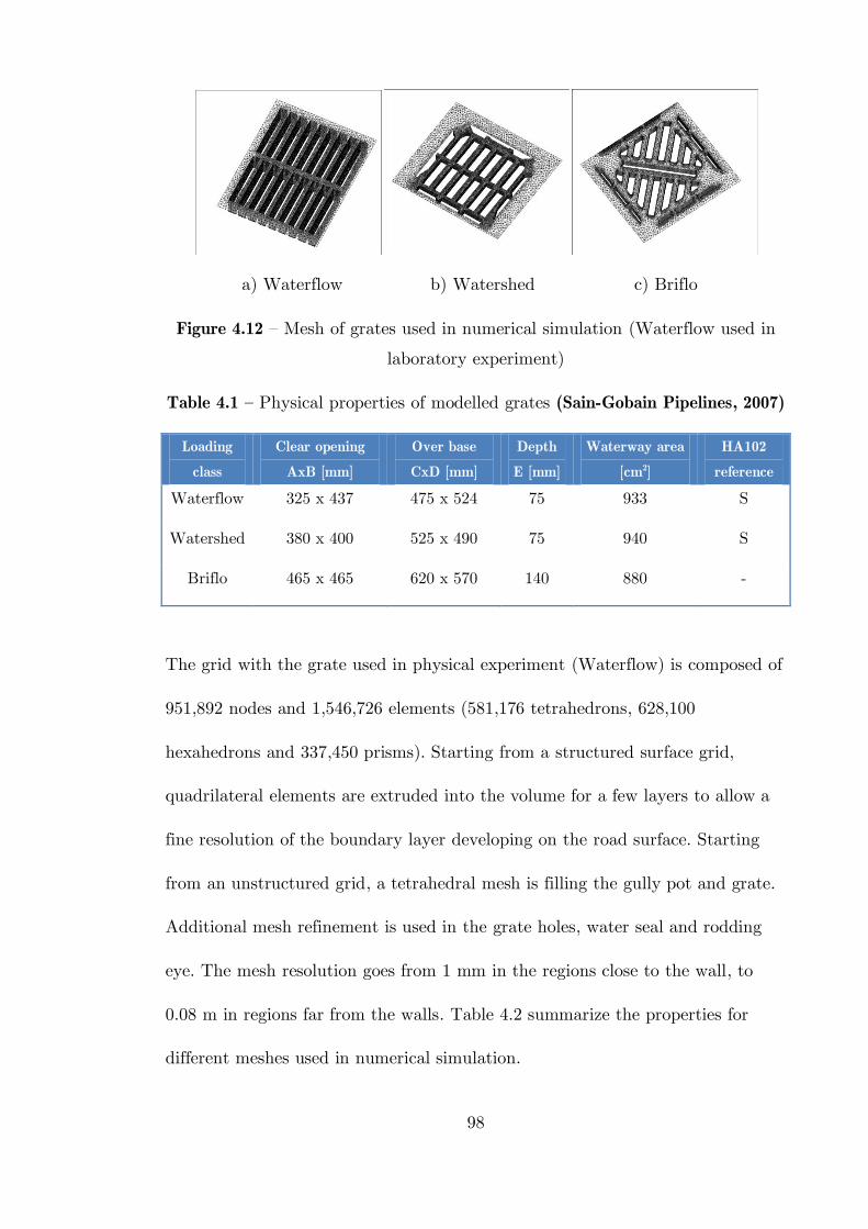
98
a) Waterflow b) Watershed c) Briflo
Figure 4.12 – Mesh of grates used in numerical simulation (Waterflow used in
laboratory experiment)
Table 4.1 – Physical properties of modelled grates (Sain-Gobain Pipelines, 2007)
Loading
class
Clear opening
AxB [mm]
Over base
CxD [mm]
Depth
E [mm]
Waterway area
[cm2]
HA102
reference
Waterflow 325 x 437 475 x 524 75 933 S
Watershed 380 x 400 525 x 490 75 940 S
Briflo 465 x 465 620 x 570 140 880 -
The grid with the grate used in physical experiment (Waterflow) is composed of
951,892 nodes and 1,546,726 elements (581,176 tetrahedrons, 628,100
hexahedrons and 337,450 prisms). Starting from a structured surface grid,
quadrilateral elements are extruded into the volume for a few layers to allow a
fine resolution of the boundary layer developing on the road surface. Starting
from an unstructured grid, a tetrahedral mesh is filling the gully pot and grate.
Additional mesh refinement is used in the grate holes, water seal and rodding
eye. The mesh resolution goes from 1 mm in the regions close to the wall, to
0.08 m in regions far from the walls. Table 4.2 summarize the properties for
different meshes used in numerical simulation.
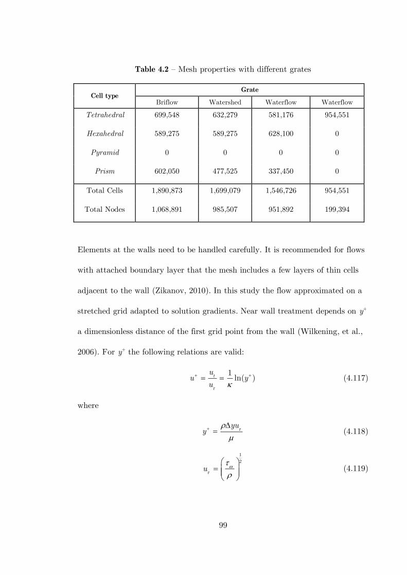
99
Table 4.2 – Mesh properties with different grates
Cell type Grate
Briflow Watershed Waterflow Waterflow
Tetrahedral 699,548 632,279 581,176 954,551
Hexahedral 589,275 589,275 628,100 0
Pyramid 0 0 0 0
Prism 602,050 477,525 337,450 0
Total Cells 1,890,873 1,699,079 1,546,726 954,551
Total Nodes 1,068,891 985,507 951,892 199,394
Elements at the walls need to be handled carefully. It is recommended for flows
with attached boundary layer that the mesh includes a few layers of thin cells
adjacent to the wall (Zikanov, 2010). In this study the flow approximated on a
stretched grid adapted to solution gradients. Near wall treatment depends on y+
a dimensionless distance of the first grid point from the wall (Wilkening, et al.,
2006). For y+ the following relations are valid:
1
ln( )tu
u yu
(4.117)
where
yu
y
(4.118)
1
2
u
(4.119)
100
u+ is the near wall velocity, uτ is the friction velocity ut is the known velocity
tangent to the wall at a distance of y from the wall, κ is the Von Karman
constant. The optimal value of y+ is lies between 5 and 10 (Andersson, et al.,
2012). As the k-ω SST turbulence model is used at walls an automatic near wall
treatment is enforced. If y+ is outside the desired range a special treatment is
applied. This has the advantage that it prevents the regeneration and
adjustment of mesh to y+ according to the geometrical and flow conditions.
4.4.3 Mesh quality
Appropriate choice of mesh type depends on the geometric complexity of
computational domain, the flow field and cell element types supported by
solver. Preparing a good initial mesh usually requires the pre-knowledge or
insight to the expected properties of the flow. The general way to eliminate the
errors is to embrace the procedure of successive refinement of an initial mesh
until certain key results shows no appreciable changes. An important aspect of
the mesh generation is choosing the appropriate size of the mesh element. The
general rule is that no fluid particle should advance through multiple mesh
elements in one time step.
In addition to mesh density the quality of a mesh depends on various criteria
such as the shape of the cells (aspect ratio, skewness, included angle of adjacent
faces), distance of cell faces from boundaries or spatial distribution of cell sizes.
The most common sources of errors are:
Mesh too coarse;
High skewness;
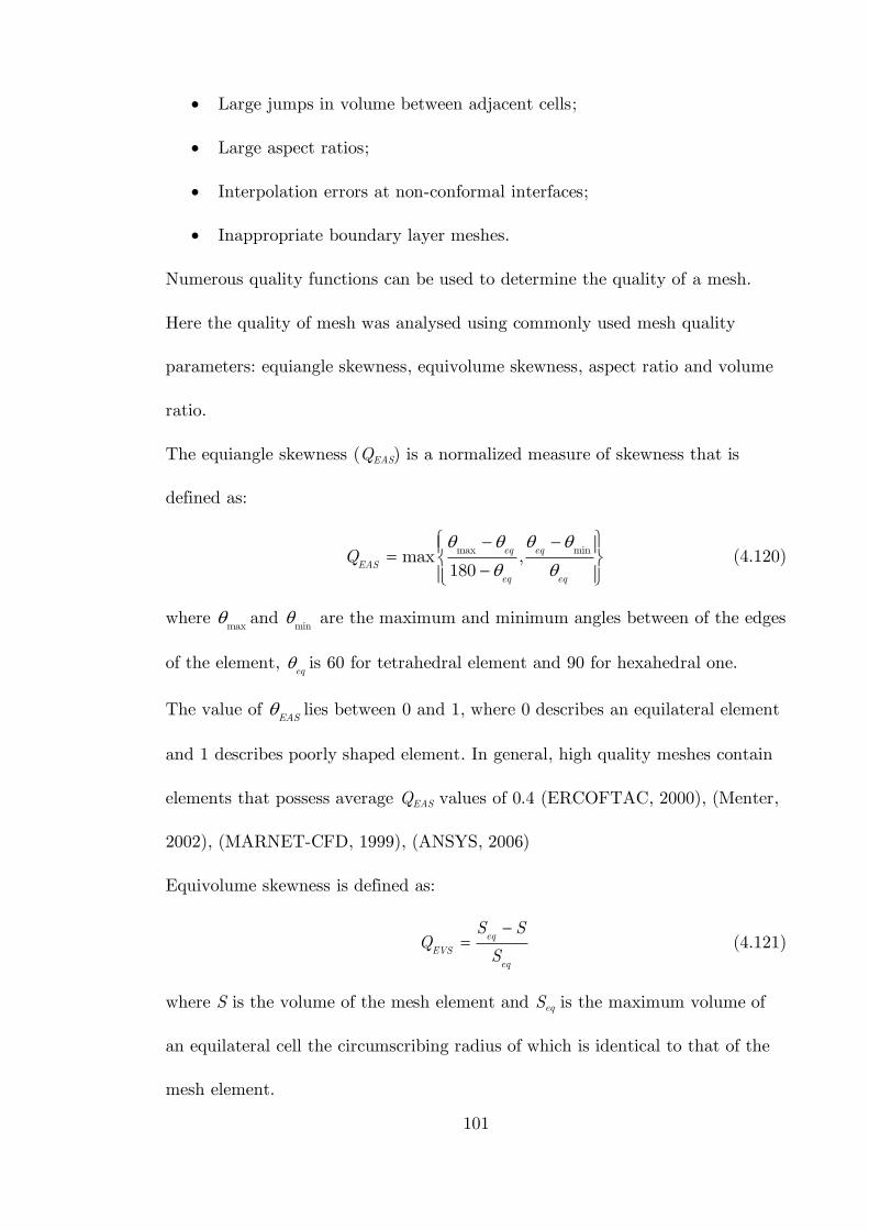
101
Large jumps in volume between adjacent cells;
Large aspect ratios;
Interpolation errors at non-conformal interfaces;
Inappropriate boundary layer meshes.
Numerous quality functions can be used to determine the quality of a mesh.
Here the quality of mesh was analysed using commonly used mesh quality
parameters: equiangle skewness, equivolume skewness, aspect ratio and volume
ratio.
The equiangle skewness (QEAS) is a normalized measure of skewness that is
defined as:
max minmax ,180
eq eq
EASeq eq
Q
(4.120)
where max and
min are the maximum and minimum angles between of the edges
of the element, eq is 60 for tetrahedral element and 90 for hexahedral one.
The value of EAS lies between 0 and 1, where 0 describes an equilateral element
and 1 describes poorly shaped element. In general, high quality meshes contain
elements that possess average QEAS values of 0.4 (ERCOFTAC, 2000), (Menter,
2002), (MARNET-CFD, 1999), (ANSYS, 2006)
Equivolume skewness is defined as:
eq
EVSeq
S SQ
S
(4.121)
where S is the volume of the mesh element and Seq is the maximum volume of
an equilateral cell the circumscribing radius of which is identical to that of the
mesh element.
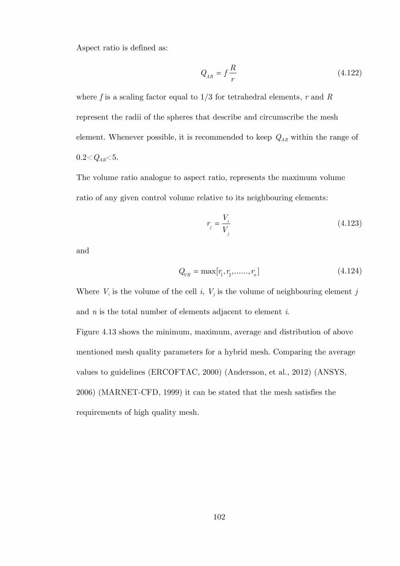
102
Aspect ratio is defined as:
AR
RQ f
r (4.122)
where f is a scaling factor equal to 1/3 for tetrahedral elements, r and R
represent the radii of the spheres that describe and circumscribe the mesh
element. Whenever possible, it is recommended to keep QAR within the range of
0.2<QAR<5.
The volume ratio analogue to aspect ratio, represents the maximum volume
ratio of any given control volume relative to its neighbouring elements:
ij
j
VrV
(4.123)
and
1 2
max[ , ,......, ]VR nQ r r r (4.124)
Where Vi is the volume of the cell i, Vj is the volume of neighbouring element j
and n is the total number of elements adjacent to element i.
Figure 4.13 shows the minimum, maximum, average and distribution of above
mentioned mesh quality parameters for a hybrid mesh. Comparing the average
values to guidelines (ERCOFTAC, 2000) (Andersson, et al., 2012) (ANSYS,
2006) (MARNET-CFD, 1999) it can be stated that the mesh satisfies the
requirements of high quality mesh.
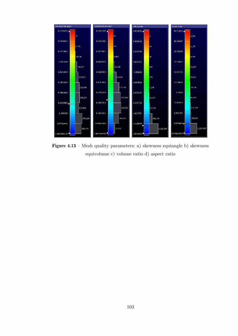
103
Figure 4.13 – Mesh quality parameters: a) skewness equiangle b) skewness
equivolume c) volume ratio d) aspect ratio
104
Chapter 5
Results
5.1 CFD Model validation
The CFD model is, like any other mathematical model, a simplified
representation of a complex physical process. The results obtained are therefore
based on many assumptions and are dependent upon the ability of the program
to successfully and accurately assimilate vast quantities of data and solve highly
complex mathematical problems. Model validation is a necessary requirement
for model application.
The effect of grid density was conducted by comparing the fine mesh results to
the ones obtained on a coarser mesh. There results were found to be close at
most locations, thought the finer mesh results gave better agreement in some
areas.
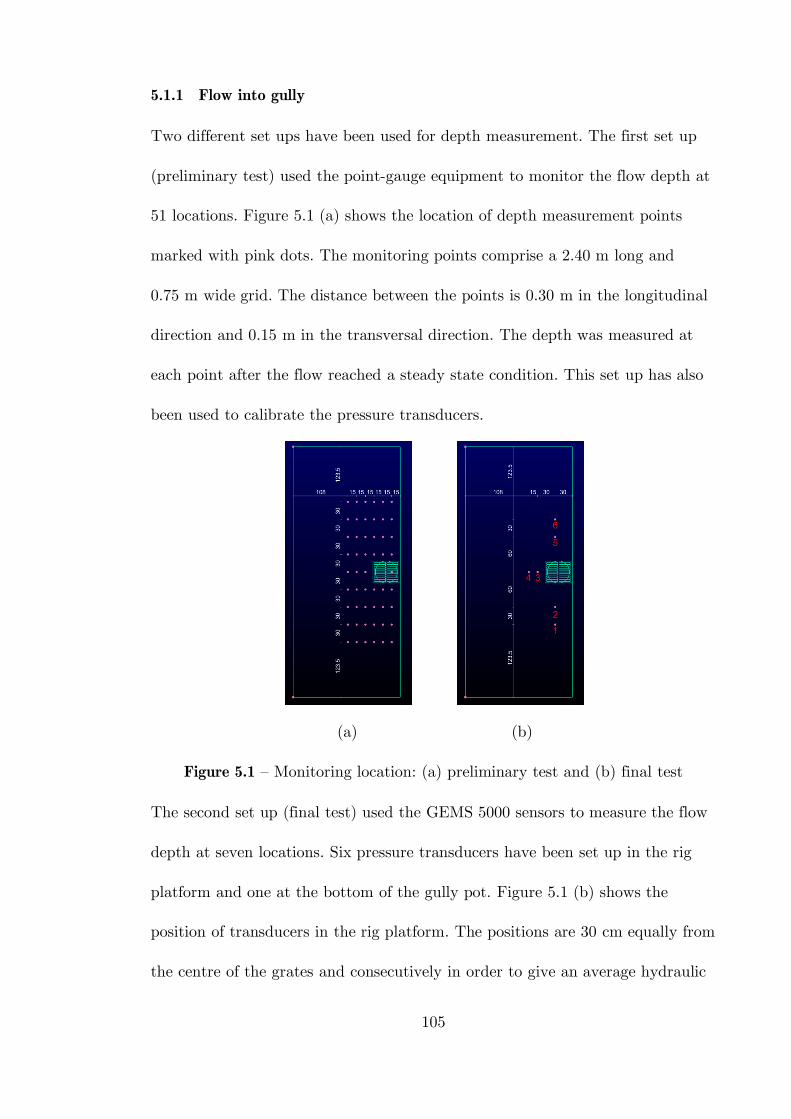
105
5.1.1 Flow into gully
Two different set ups have been used for depth measurement. The first set up
(preliminary test) used the point-gauge equipment to monitor the flow depth at
51 locations. Figure 5.1 (a) shows the location of depth measurement points
marked with pink dots. The monitoring points comprise a 2.40 m long and
0.75 m wide grid. The distance between the points is 0.30 m in the longitudinal
direction and 0.15 m in the transversal direction. The depth was measured at
each point after the flow reached a steady state condition. This set up has also
been used to calibrate the pressure transducers.
(a) (b)
Figure 5.1 – Monitoring location: (a) preliminary test and (b) final test
The second set up (final test) used the GEMS 5000 sensors to measure the flow
depth at seven locations. Six pressure transducers have been set up in the rig
platform and one at the bottom of the gully pot. Figure 5.1 (b) shows the
position of transducers in the rig platform. The positions are 30 cm equally from
the centre of the grates and consecutively in order to give an average hydraulic
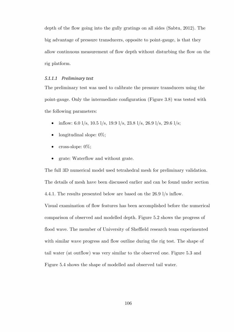
106
depth of the flow going into the gully gratings on all sides (Sabtu, 2012). The
big advantage of pressure transducers, opposite to point-gauge, is that they
allow continuous measurement of flow depth without disturbing the flow on the
rig platform.
5.1.1.1 Preliminary test
The preliminary test was used to calibrate the pressure transducers using the
point-gauge. Only the intermediate configuration (Figure 3.8) was tested with
the following parameters:
inflow: 6.0 l/s, 10.5 l/s, 19.9 l/s, 23.8 l/s, 26.9 l/s, 29.6 l/s;
longitudinal slope: 0%;
cross-slope: 0%;
grate: Waterflow and without grate.
The full 3D numerical model used tetrahedral mesh for preliminary validation.
The details of mesh have been discussed earlier and can be found under section
4.4.1. The results presented below are based on the 26.9 l/s inflow.
Visual examination of flow features has been accomplished before the numerical
comparison of observed and modelled depth. Figure 5.2 shows the progress of
flood wave. The member of University of Sheffield research team experimented
with similar wave progress and flow outline during the rig test. The shape of
tail water (at outflow) was very similar to the observed one. Figure 5.3 and
Figure 5.4 shows the shape of modelled and observed tail water.
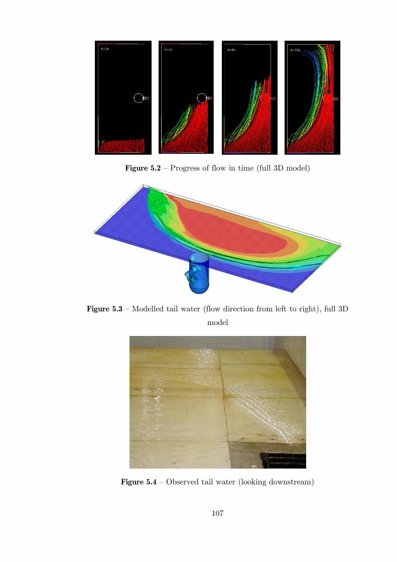
107
Figure 5.2 – Progress of flow in time (full 3D model)
Figure 5.3 – Modelled tail water (flow direction from left to right), full 3D
model
Figure 5.4 – Observed tail water (looking downstream)
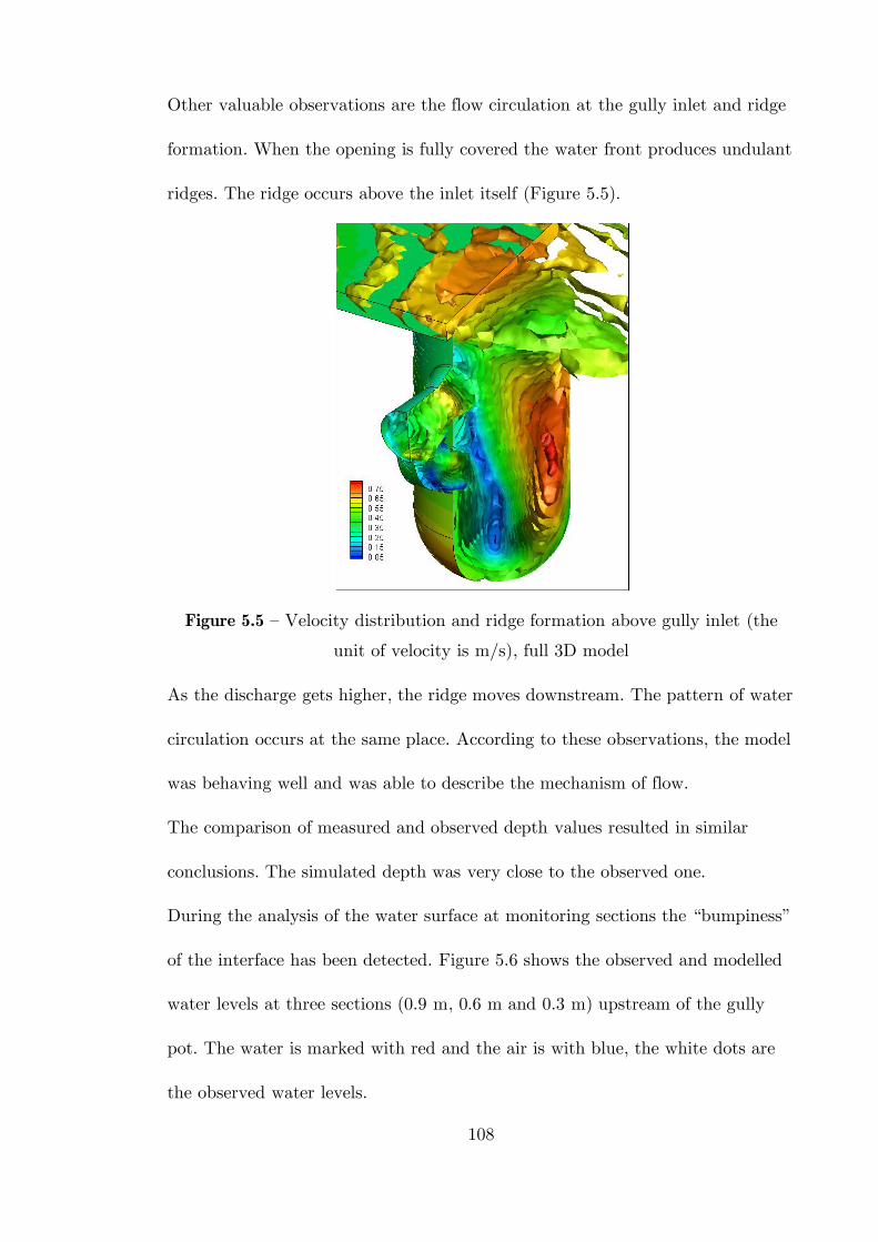
108
Other valuable observations are the flow circulation at the gully inlet and ridge
formation. When the opening is fully covered the water front produces undulant
ridges. The ridge occurs above the inlet itself (Figure 5.5).
Figure 5.5 – Velocity distribution and ridge formation above gully inlet (the
unit of velocity is m/s), full 3D model
As the discharge gets higher, the ridge moves downstream. The pattern of water
circulation occurs at the same place. According to these observations, the model
was behaving well and was able to describe the mechanism of flow.
The comparison of measured and observed depth values resulted in similar
conclusions. The simulated depth was very close to the observed one.
During the analysis of the water surface at monitoring sections the “bumpiness”
of the interface has been detected. Figure 5.6 shows the observed and modelled
water levels at three sections (0.9 m, 0.6 m and 0.3 m) upstream of the gully
pot. The water is marked with red and the air is with blue, the white dots are
the observed water levels.
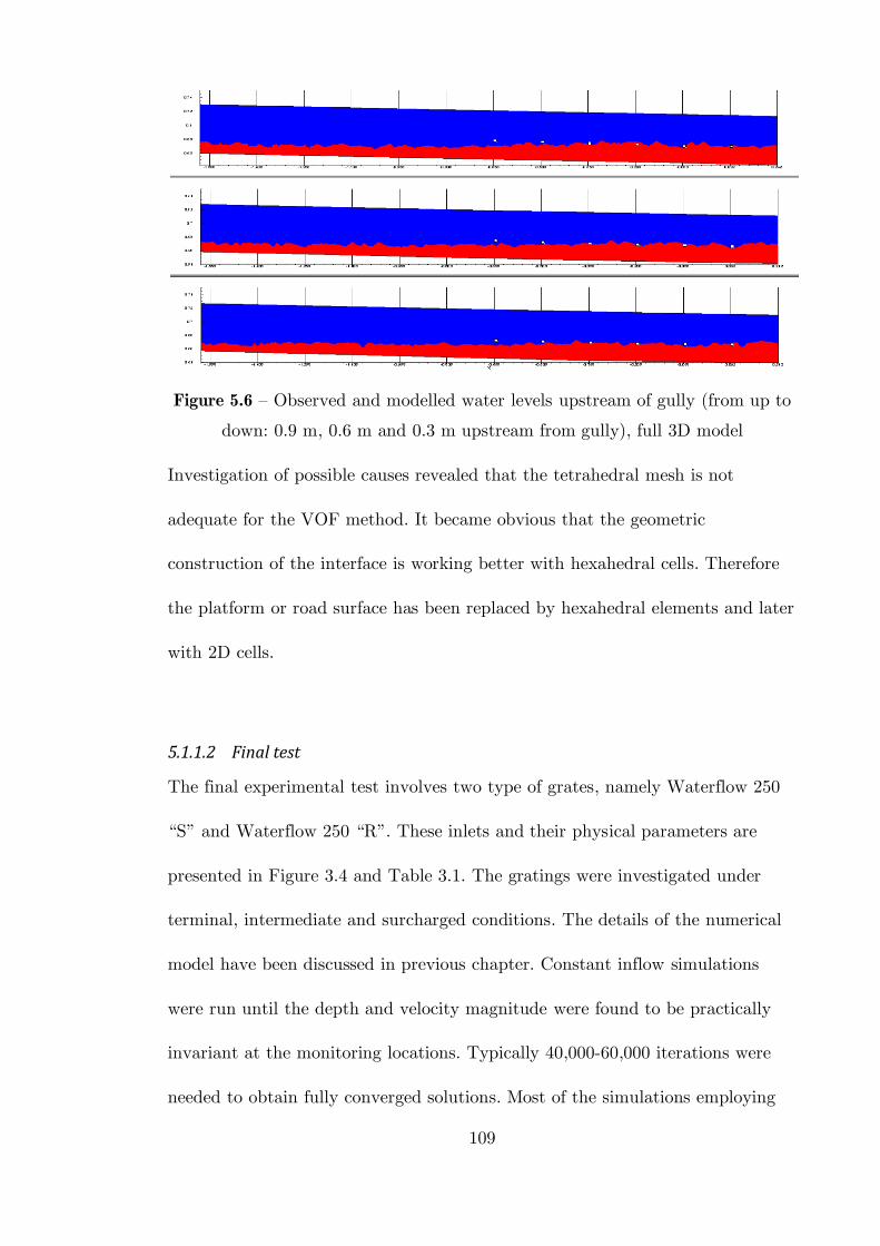
109
Figure 5.6 – Observed and modelled water levels upstream of gully (from up to
down: 0.9 m, 0.6 m and 0.3 m upstream from gully), full 3D model
Investigation of possible causes revealed that the tetrahedral mesh is not
adequate for the VOF method. It became obvious that the geometric
construction of the interface is working better with hexahedral cells. Therefore
the platform or road surface has been replaced by hexahedral elements and later
with 2D cells.
5.1.1.2 Final test
The final experimental test involves two type of grates, namely Waterflow 250
“S” and Waterflow 250 “R”. These inlets and their physical parameters are
presented in Figure 3.4 and Table 3.1. The gratings were investigated under
terminal, intermediate and surcharged conditions. The details of the numerical
model have been discussed in previous chapter. Constant inflow simulations
were run until the depth and velocity magnitude were found to be practically
invariant at the monitoring locations. Typically 40,000-60,000 iterations were
needed to obtain fully converged solutions. Most of the simulations employing
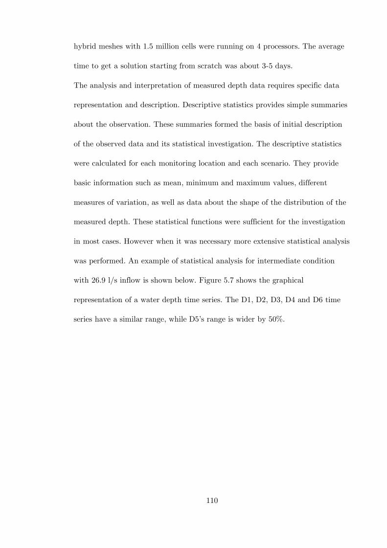
110
hybrid meshes with 1.5 million cells were running on 4 processors. The average
time to get a solution starting from scratch was about 3-5 days.
The analysis and interpretation of measured depth data requires specific data
representation and description. Descriptive statistics provides simple summaries
about the observation. These summaries formed the basis of initial description
of the observed data and its statistical investigation. The descriptive statistics
were calculated for each monitoring location and each scenario. They provide
basic information such as mean, minimum and maximum values, different
measures of variation, as well as data about the shape of the distribution of the
measured depth. These statistical functions were sufficient for the investigation
in most cases. However when it was necessary more extensive statistical analysis
was performed. An example of statistical analysis for intermediate condition
with 26.9 l/s inflow is shown below. Figure 5.7 shows the graphical
representation of a water depth time series. The D1, D2, D3, D4 and D6 time
series have a similar range, while D5’s range is wider by 50%.
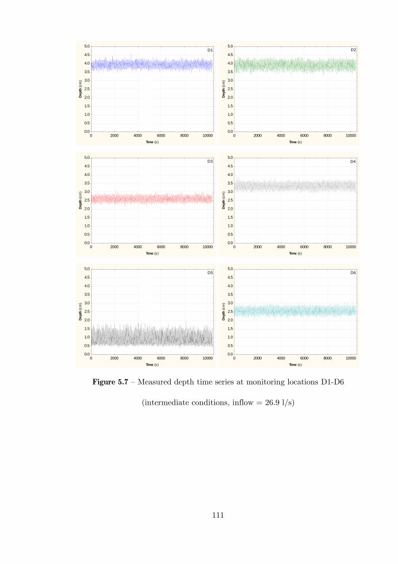
111
0 2000 4000 6000 8000 10000
Time (s)
0.0
0.5
1.0
1.5
2.0
2.5
3.0
3.5
4.0
4.5
5.0
De
pth
(c
m)
D1
0 2000 4000 6000 8000 10000
Time (s)
0.0
0.5
1.0
1.5
2.0
2.5
3.0
3.5
4.0
4.5
5.0
De
pth
(c
m)
D2
0 2000 4000 6000 8000 10000
Time (s)
0.0
0.5
1.0
1.5
2.0
2.5
3.0
3.5
4.0
4.5
5.0
De
pth
(c
m)
D3
0 2000 4000 6000 8000 10000
Time (s)
0.0
0.5
1.0
1.5
2.0
2.5
3.0
3.5
4.0
4.5
5.0
De
pth
(c
m)
D4
0 2000 4000 6000 8000 10000
Time (s)
0.0
0.5
1.0
1.5
2.0
2.5
3.0
3.5
4.0
4.5
5.0
De
pth
(c
m)
D5
0 2000 4000 6000 8000 10000
Time (s)
0.0
0.5
1.0
1.5
2.0
2.5
3.0
3.5
4.0
4.5
5.0
De
pth
(c
m)
D6
Figure 5.7 – Measured depth time series at monitoring locations D1-D6
(intermediate conditions, inflow = 26.9 l/s)
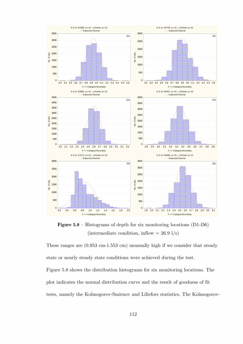
112
K-S d=.04385, p<.01 ; Lilliefors p<.01
Expected Normal
3.3 3.4 3.5 3.6 3.7 3.8 3.9 4.0 4.1 4.2 4.3 4.4 4.5 4.6
X <= Category Boundary
0
500
1000
1500
2000
2500
3000
3500
No
. o
f o
bs
.
D1
K-S d=.03745, p<.01 ; Lilliefors p<.01
Expected Normal
3.2 3.3 3.4 3.5 3.6 3.7 3.8 3.9 4.0 4.1 4.2 4.3 4.4 4.5
X <= Category Boundary
0
500
1000
1500
2000
2500
3000
No
. o
f o
bs
.
D2
K-S d=.03982, p<.01 ; Lilliefors p<.01
Expected Normal
2.0 2.1 2.2 2.3 2.4 2.5 2.6 2.7 2.8 2.9 3.0 3.1 3.2
X <= Category Boundary
0
500
1000
1500
2000
2500
3000
3500
4000
4500
No
. o
f o
bs
.
D3
K-S d=.04057, p<.01 ; Lilliefors p<.01
Expected Normal
2.8 2.9 3.0 3.1 3.2 3.3 3.4 3.5 3.6 3.7 3.8 3.9
X <= Category Boundary
0
500
1000
1500
2000
2500
3000
3500
4000
No
. o
f o
bs
.
D4
K-S d=.12274, p<.01 ; Lilliefors p<.01
Expected Normal
0.2 0.4 0.6 0.8 1.0 1.2 1.4 1.6 1.8 2.0
X <= Category Boundary
0
500
1000
1500
2000
2500
3000
No
. o
f o
bs
.
D5
K-S d=.03680, p<.01 ; Lilliefors p<.01
Expected Normal
1.9 2.0 2.1 2.2 2.3 2.4 2.5 2.6 2.7 2.8 2.9 3.0 3.1
X <= Category Boundary
0
500
1000
1500
2000
2500
3000
3500
No
. o
f o
bs
.
D6
Figure 5.8 – Histograms of depth for six monitoring locations (D1-D6)
(intermediate condition, inflow = 26.9 l/s)
These ranges are (0.953 cm-1.553 cm) unusually high if we consider that steady
state or nearly steady state conditions were achieved during the test.
Figure 5.8 shows the distribution histograms for six monitoring locations. The
plot indicates the normal distribution curve and the result of goodness of fit
tests, namely the Kolmogorov-Smirnov and Liliefors statistics. The Kolmogorov-
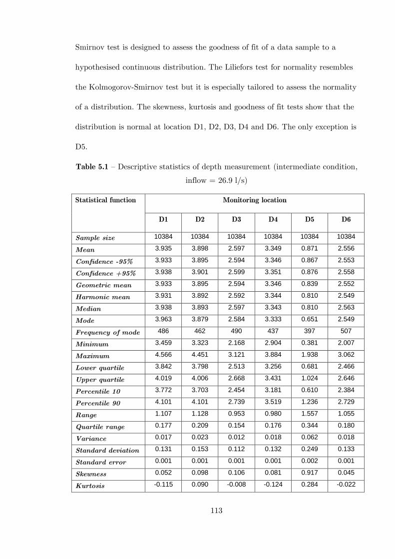
113
Smirnov test is designed to assess the goodness of fit of a data sample to a
hypothesised continuous distribution. The Liliefors test for normality resembles
the Kolmogorov-Smirnov test but it is especially tailored to assess the normality
of a distribution. The skewness, kurtosis and goodness of fit tests show that the
distribution is normal at location D1, D2, D3, D4 and D6. The only exception is
D5.
Table 5.1 – Descriptive statistics of depth measurement (intermediate condition,
inflow = 26.9 l/s)
Statistical function Monitoring location
D1 D2 D3 D4 D5 D6
Sample size 10384 10384 10384 10384 10384 10384
Mean 3.935 3.898 2.597 3.349 0.871 2.556
Confidence -95% 3.933 3.895 2.594 3.346 0.867 2.553
Confidence +95% 3.938 3.901 2.599 3.351 0.876 2.558
Geometric mean 3.933 3.895 2.594 3.346 0.839 2.552
Harmonic mean 3.931 3.892 2.592 3.344 0.810 2.549
Median 3.938 3.893 2.597 3.343 0.810 2.563
Mode 3.963 3.879 2.584 3.333 0.651 2.549
Frequency of mode 486 462 490 437 397 507
Minimum 3.459 3.323 2.168 2.904 0.381 2.007
Maximum 4.566 4.451 3.121 3.884 1.938 3.062
Lower quartile 3.842 3.798 2.513 3.256 0.681 2.466
Upper quartile 4.019 4.006 2.668 3.431 1.024 2.646
Percentile 10 3.772 3.703 2.454 3.181 0.610 2.384
Percentile 90 4.101 4.101 2.739 3.519 1.236 2.729
Range 1.107 1.128 0.953 0.980 1.557 1.055
Quartile range 0.177 0.209 0.154 0.176 0.344 0.180
Variance 0.017 0.023 0.012 0.018 0.062 0.018
Standard deviation 0.131 0.153 0.112 0.132 0.249 0.133
Standard error 0.001 0.001 0.001 0.001 0.002 0.001
Skewness 0.052 0.098 0.106 0.081 0.917 0.045
Kurtosis -0.115 0.090 -0.008 -0.124 0.284 -0.022
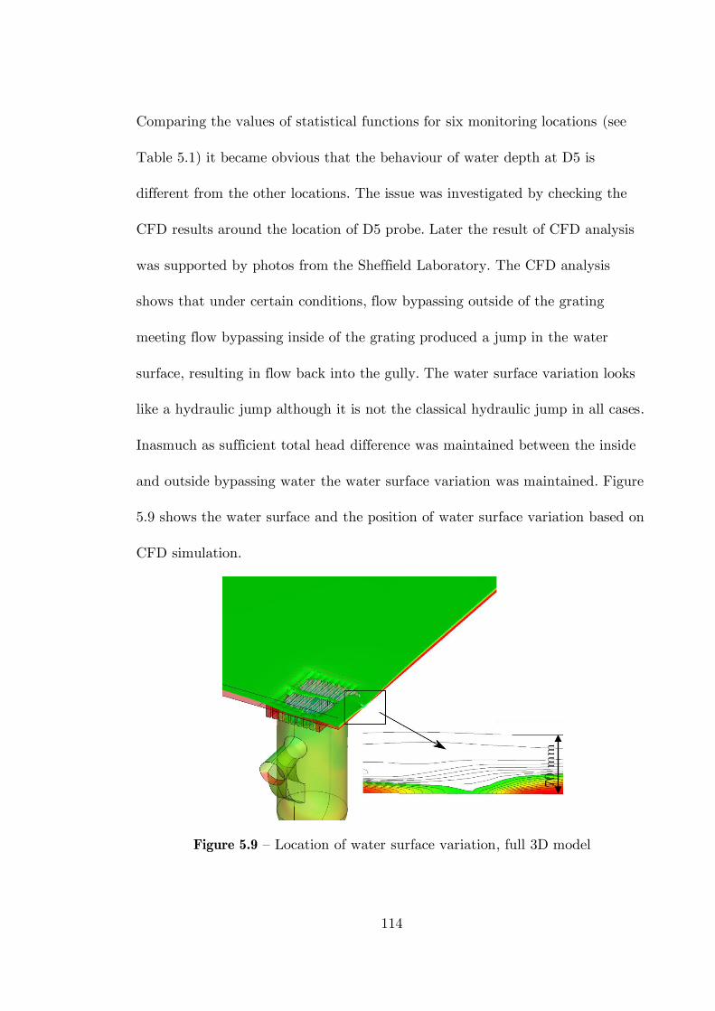
114
Comparing the values of statistical functions for six monitoring locations (see
Table 5.1) it became obvious that the behaviour of water depth at D5 is
different from the other locations. The issue was investigated by checking the
CFD results around the location of D5 probe. Later the result of CFD analysis
was supported by photos from the Sheffield Laboratory. The CFD analysis
shows that under certain conditions, flow bypassing outside of the grating
meeting flow bypassing inside of the grating produced a jump in the water
surface, resulting in flow back into the gully. The water surface variation looks
like a hydraulic jump although it is not the classical hydraulic jump in all cases.
Inasmuch as sufficient total head difference was maintained between the inside
and outside bypassing water the water surface variation was maintained. Figure
5.9 shows the water surface and the position of water surface variation based on
CFD simulation.
Figure 5.9 – Location of water surface variation, full 3D model
70 m
m
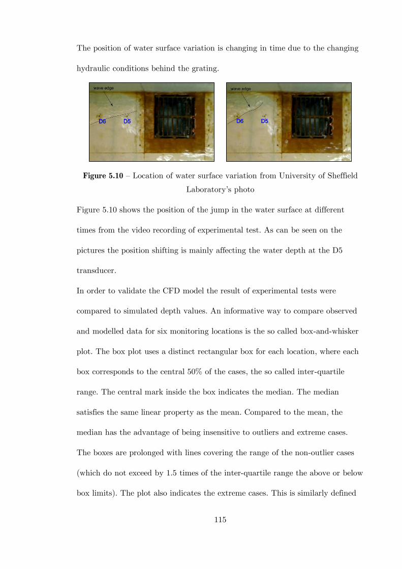
115
The position of water surface variation is changing in time due to the changing
hydraulic conditions behind the grating.
Figure 5.10 – Location of water surface variation from University of Sheffield
Laboratory’s photo
Figure 5.10 shows the position of the jump in the water surface at different
times from the video recording of experimental test. As can be seen on the
pictures the position shifting is mainly affecting the water depth at the D5
transducer.
In order to validate the CFD model the result of experimental tests were
compared to simulated depth values. An informative way to compare observed
and modelled data for six monitoring locations is the so called box-and-whisker
plot. The box plot uses a distinct rectangular box for each location, where each
box corresponds to the central 50% of the cases, the so called inter-quartile
range. The central mark inside the box indicates the median. The median
satisfies the same linear property as the mean. Compared to the mean, the
median has the advantage of being insensitive to outliers and extreme cases.
The boxes are prolonged with lines covering the range of the non-outlier cases
(which do not exceed by 1.5 times of the inter-quartile range the above or below
box limits). The plot also indicates the extreme cases. This is similarly defined
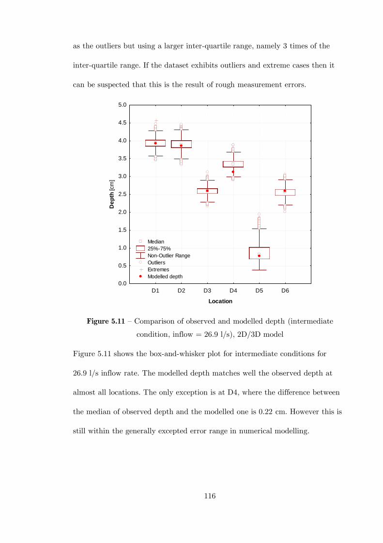
116
as the outliers but using a larger inter-quartile range, namely 3 times of the
inter-quartile range. If the dataset exhibits outliers and extreme cases then it
can be suspected that this is the result of rough measurement errors.
D1 D2 D3 D4 D5 D6
Location
0.0
0.5
1.0
1.5
2.0
2.5
3.0
3.5
4.0
4.5
5.0D
ep
th [cm
]
Median
25%-75%
Non-Outlier Range
Outliers
Extremes
Modelled depth
Figure 5.11 – Comparison of observed and modelled depth (intermediate
condition, inflow = 26.9 l/s), 2D/3D model
Figure 5.11 shows the box-and-whisker plot for intermediate conditions for
26.9 l/s inflow rate. The modelled depth matches well the observed depth at
almost all locations. The only exception is at D4, where the difference between
the median of observed depth and the modelled one is 0.22 cm. However this is
still within the generally excepted error range in numerical modelling.
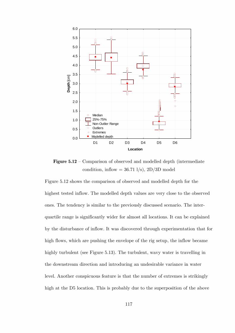
117
D1 D2 D3 D4 D5 D6
Location
0.0
0.5
1.0
1.5
2.0
2.5
3.0
3.5
4.0
4.5
5.0
5.5
6.0
De
pth
[cm
]
Median
25%-75%
Non-Outlier Range
Outliers
Extremes
Modelled depth
Figure 5.12 – Comparison of observed and modelled depth (intermediate
condition, inflow = 36.71 l/s), 2D/3D model
Figure 5.12 shows the comparison of observed and modelled depth for the
highest tested inflow. The modelled depth values are very close to the observed
ones. The tendency is similar to the previously discussed scenario. The inter-
quartile range is significantly wider for almost all locations. It can be explained
by the disturbance of inflow. It was discovered through experimentation that for
high flows, which are pushing the envelope of the rig setup, the inflow became
highly turbulent (see Figure 5.13). The turbulent, wavy water is travelling in
the downstream direction and introducing an undesirable variance in water
level. Another conspicuous feature is that the number of extremes is strikingly
high at the D5 location. This is probably due to the superposition of the above
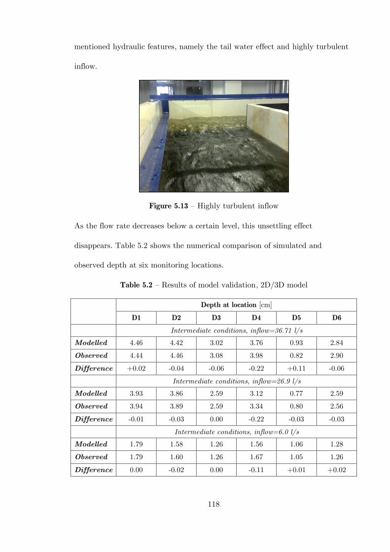
118
mentioned hydraulic features, namely the tail water effect and highly turbulent
inflow.
Figure 5.13 – Highly turbulent inflow
As the flow rate decreases below a certain level, this unsettling effect
disappears. Table 5.2 shows the numerical comparison of simulated and
observed depth at six monitoring locations.
Table 5.2 – Results of model validation, 2D/3D model
Depth at location [cm]
D1 D2 D3 D4 D5 D6
Intermediate conditions, inflow=36.71 l/s
Modelled 4.46 4.42 3.02 3.76 0.93 2.84
Observed 4.44 4.46 3.08 3.98 0.82 2.90
Difference +0.02 -0.04 -0.06 -0.22 +0.11 -0.06
Intermediate conditions, inflow=26.9 l/s
Modelled 3.93 3.86 2.59 3.12 0.77 2.59
Observed 3.94 3.89 2.59 3.34 0.80 2.56
Difference -0.01 -0.03 0.00 -0.22 -0.03 -0.03
Intermediate conditions, inflow=6.0 l/s
Modelled 1.79 1.58 1.26 1.56 1.06 1.28
Observed 1.79 1.60 1.26 1.67 1.05 1.26
Difference 0.00 -0.02 0.00 -0.11 +0.01 +0.02
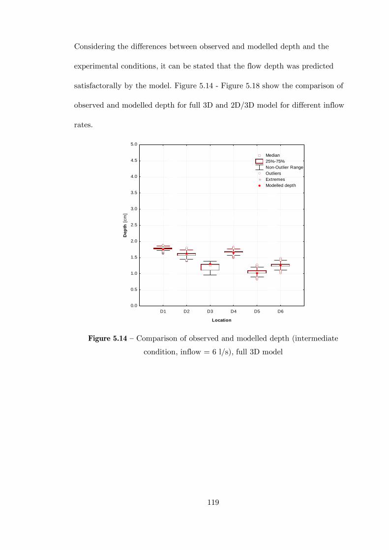
119
Considering the differences between observed and modelled depth and the
experimental conditions, it can be stated that the flow depth was predicted
satisfactorally by the model. Figure 5.14 - Figure 5.18 show the comparison of
observed and modelled depth for full 3D and 2D/3D model for different inflow
rates.
D1 D2 D3 D4 D5 D6
Location
0.0
0.5
1.0
1.5
2.0
2.5
3.0
3.5
4.0
4.5
5.0
Dep
th [
cm
]
Median
25%-75%
Non-Outlier Range
Outliers
Extremes
Modelled depth
Figure 5.14 – Comparison of observed and modelled depth (intermediate
condition, inflow = 6 l/s), full 3D model
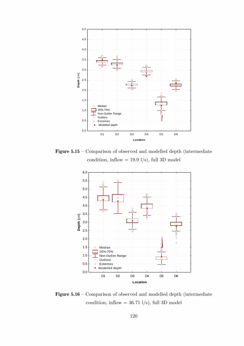
120
D1 D2 D3 D4 D5 D6
Location
0.0
0.5
1.0
1.5
2.0
2.5
3.0
3.5
4.0
4.5
5.0
Dep
th [
cm
]
Median
25%-75%
Non-Outlier Range
Outliers
Extremes
Modelled depth
Figure 5.15 – Comparison of observed and modelled depth (intermediate
condition, inflow = 19.9 l/s), full 3D model
D1 D2 D3 D4 D5 D6
Location
0.0
0.5
1.0
1.5
2.0
2.5
3.0
3.5
4.0
4.5
5.0
5.5
6.0
Dep
th [cm
]
Median
25%-75%
Non-Outlier Range
Outliers
Extremes
Modelled depth
Figure 5.16 – Comparison of observed and modelled depth (intermediate
condition, inflow = 36.71 l/s), full 3D model
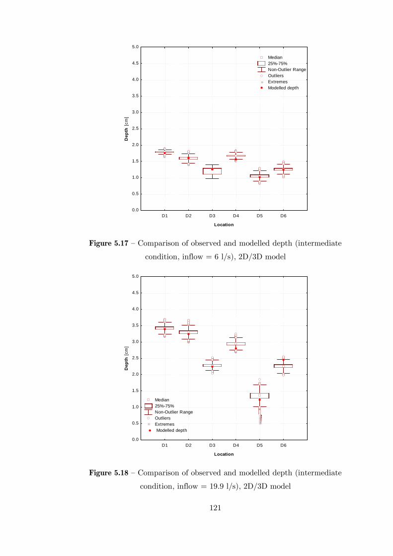
121
D1 D2 D3 D4 D5 D6
Location
0.0
0.5
1.0
1.5
2.0
2.5
3.0
3.5
4.0
4.5
5.0
Dep
th [
cm
]
Median
25%-75%
Non-Outlier Range
Outliers
Extremes
Modelled depth
Figure 5.17 – Comparison of observed and modelled depth (intermediate
condition, inflow = 6 l/s), 2D/3D model
D1 D2 D3 D4 D5 D6
Location
0.0
0.5
1.0
1.5
2.0
2.5
3.0
3.5
4.0
4.5
5.0
Dep
th [
cm
]
Median
25%-75%
Non-Outlier Range
Outliers
Extremes
Modelled depth
Figure 5.18 – Comparison of observed and modelled depth (intermediate
condition, inflow = 19.9 l/s), 2D/3D model
122
5.1.2 Surcharged gully
According to EN 752 “flooding” describes a “condition where wastewater
and/or surface water escapes from or cannot enter a drain or sewer system and
either remains on the surface or enters buildings”. The term “surcharge” is
defined as a “condition in which wastewater and/or surface water is held under
pressure within a gravity drain or sewer systems, but does not escape to the
surface to cause flooding”. Eventually surcharge conditions may lead to a rise of
water level above the surface. In this case the water escapes from the drain
system or prevents surface water from entering into the drain system (Schmitt,
et al., 2004). The surcharging condition has occurred more frequently in the last
decade causing severe disruption of urban transport. However, to the author's
knowledge no studies have been carried out to quantify this effect.
The details of surcharging conditions were discussed in Chapter 3. Figure 3.9
shows the schematic of surcharged system. The validation started with visual
comparison of water surface obtained from physical experiment and CFD
modelling. Figure 5.19 shows the modelled and observed surcharging water
levels. The visual comparison of water surface features is challenging due to the
transparency of the water. However it can be stated that the modelled water
surface is similar to the observed one.
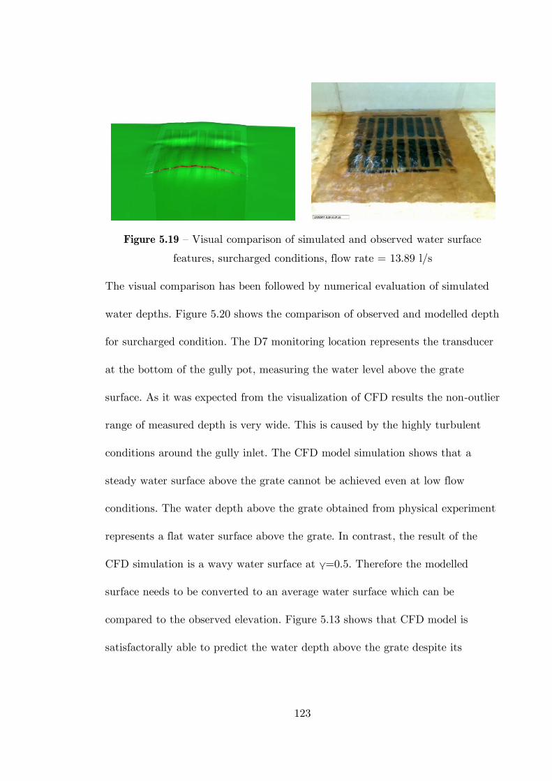
123
Figure 5.19 – Visual comparison of simulated and observed water surface
features, surcharged conditions, flow rate = 13.89 l/s
The visual comparison has been followed by numerical evaluation of simulated
water depths. Figure 5.20 shows the comparison of observed and modelled depth
for surcharged condition. The D7 monitoring location represents the transducer
at the bottom of the gully pot, measuring the water level above the grate
surface. As it was expected from the visualization of CFD results the non-outlier
range of measured depth is very wide. This is caused by the highly turbulent
conditions around the gully inlet. The CFD model simulation shows that a
steady water surface above the grate cannot be achieved even at low flow
conditions. The water depth above the grate obtained from physical experiment
represents a flat water surface above the grate. In contrast, the result of the
CFD simulation is a wavy water surface at γ=0.5. Therefore the modelled
surface needs to be converted to an average water surface which can be
compared to the observed elevation. Figure 5.13 shows that CFD model is
satisfactorally able to predict the water depth above the grate despite its
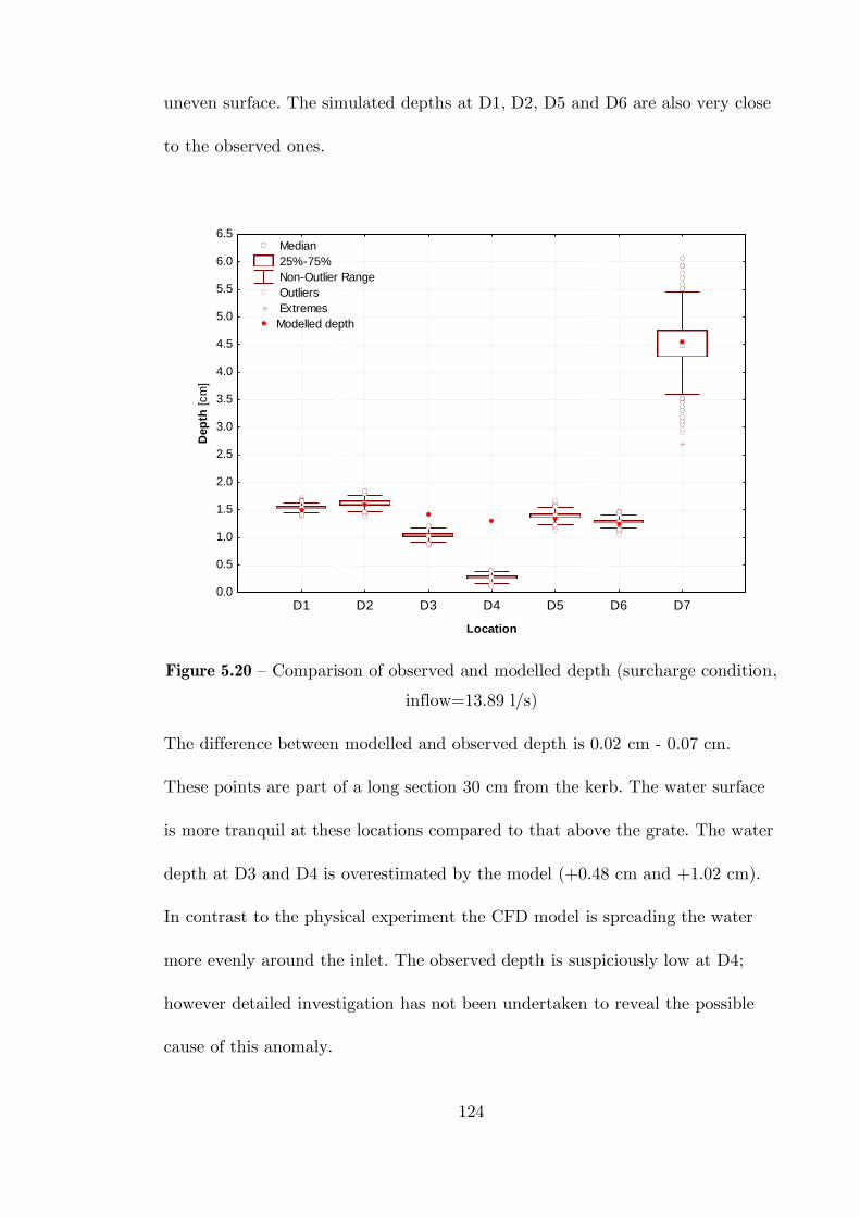
124
uneven surface. The simulated depths at D1, D2, D5 and D6 are also very close
to the observed ones.
D1 D2 D3 D4 D5 D6 D7
Location
0.0
0.5
1.0
1.5
2.0
2.5
3.0
3.5
4.0
4.5
5.0
5.5
6.0
6.5
Dep
th [cm
]
Median
25%-75%
Non-Outlier Range
Outliers
Extremes
Modelled depth
Figure 5.20 – Comparison of observed and modelled depth (surcharge condition,
inflow=13.89 l/s)
The difference between modelled and observed depth is 0.02 cm - 0.07 cm.
These points are part of a long section 30 cm from the kerb. The water surface
is more tranquil at these locations compared to that above the grate. The water
depth at D3 and D4 is overestimated by the model (+0.48 cm and +1.02 cm).
In contrast to the physical experiment the CFD model is spreading the water
more evenly around the inlet. The observed depth is suspiciously low at D4;
however detailed investigation has not been undertaken to reveal the possible
cause of this anomaly.
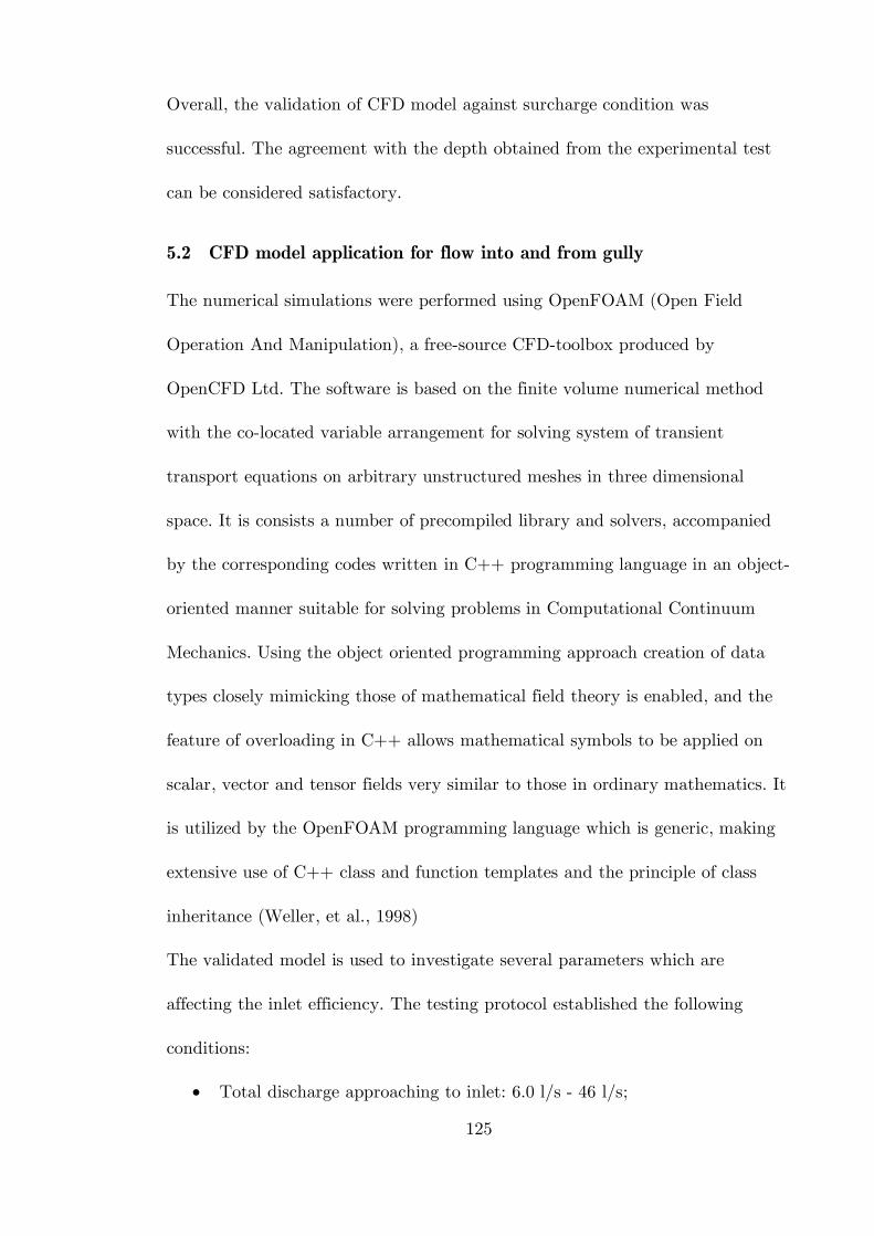
125
Overall, the validation of CFD model against surcharge condition was
successful. The agreement with the depth obtained from the experimental test
can be considered satisfactory.
5.2 CFD model application for flow into and from gully
The numerical simulations were performed using OpenFOAM (Open Field
Operation And Manipulation), a free-source CFD-toolbox produced by
OpenCFD Ltd. The software is based on the finite volume numerical method
with the co-located variable arrangement for solving system of transient
transport equations on arbitrary unstructured meshes in three dimensional
space. It is consists a number of precompiled library and solvers, accompanied
by the corresponding codes written in C++ programming language in an object-
oriented manner suitable for solving problems in Computational Continuum
Mechanics. Using the object oriented programming approach creation of data
types closely mimicking those of mathematical field theory is enabled, and the
feature of overloading in C++ allows mathematical symbols to be applied on
scalar, vector and tensor fields very similar to those in ordinary mathematics. It
is utilized by the OpenFOAM programming language which is generic, making
extensive use of C++ class and function templates and the principle of class
inheritance (Weller, et al., 1998)
The validated model is used to investigate several parameters which are
affecting the inlet efficiency. The testing protocol established the following
conditions:
Total discharge approaching to inlet: 6.0 l/s - 46 l/s;
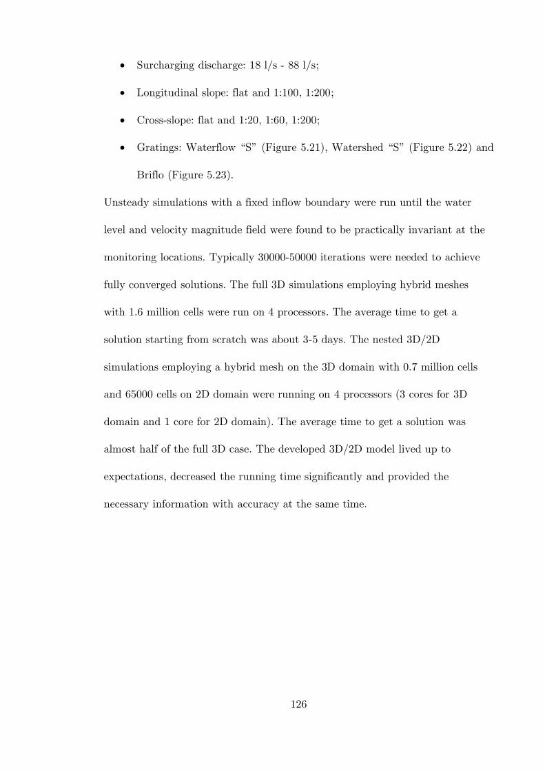
126
Surcharging discharge: 18 l/s - 88 l/s;
Longitudinal slope: flat and 1:100, 1:200;
Cross-slope: flat and 1:20, 1:60, 1:200;
Gratings: Waterflow “S” (Figure 5.21), Watershed “S” (Figure 5.22) and
Briflo (Figure 5.23).
Unsteady simulations with a fixed inflow boundary were run until the water
level and velocity magnitude field were found to be practically invariant at the
monitoring locations. Typically 30000-50000 iterations were needed to achieve
fully converged solutions. The full 3D simulations employing hybrid meshes
with 1.6 million cells were run on 4 processors. The average time to get a
solution starting from scratch was about 3-5 days. The nested 3D/2D
simulations employing a hybrid mesh on the 3D domain with 0.7 million cells
and 65000 cells on 2D domain were running on 4 processors (3 cores for 3D
domain and 1 core for 2D domain). The average time to get a solution was
almost half of the full 3D case. The developed 3D/2D model lived up to
expectations, decreased the running time significantly and provided the
necessary information with accuracy at the same time.
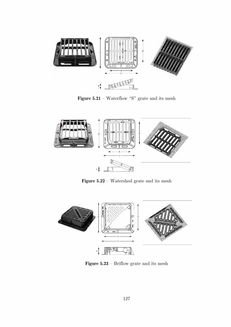
127
Figure 5.21 – Waterflow “S” grate and its mesh
Figure 5.22 – Watershed grate and its mesh
Figure 5.23 – Briflow grate and its mesh
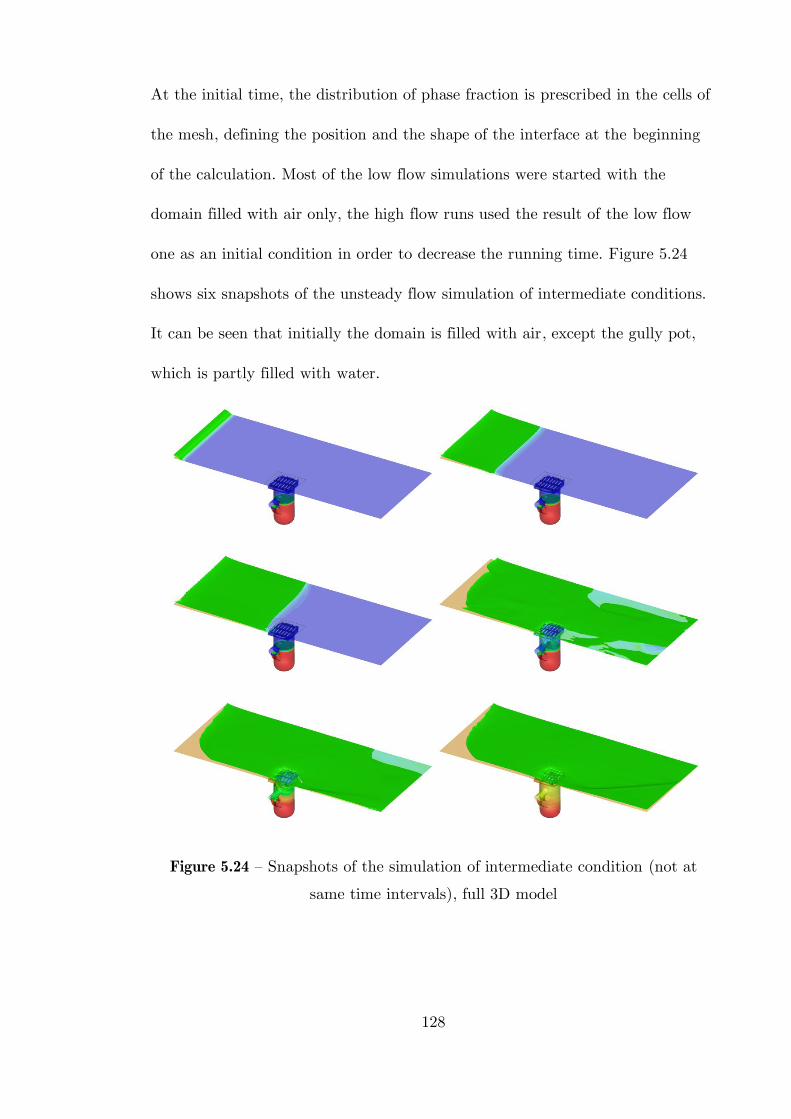
128
At the initial time, the distribution of phase fraction is prescribed in the cells of
the mesh, defining the position and the shape of the interface at the beginning
of the calculation. Most of the low flow simulations were started with the
domain filled with air only, the high flow runs used the result of the low flow
one as an initial condition in order to decrease the running time. Figure 5.24
shows six snapshots of the unsteady flow simulation of intermediate conditions.
It can be seen that initially the domain is filled with air, except the gully pot,
which is partly filled with water.
Figure 5.24 – Snapshots of the simulation of intermediate condition (not at
same time intervals), full 3D model
129
The aim of this initial condition for the gully was to reduce the filling time of
gully pot hereby decreasing the running time.
The water is entering the plate at the left edge and flowing to right. The front
wave remains almost perpendicular to the curb due to the flat long slope and
cross slope (first row picture one and picture two, second row picture one). One
part of the approaching front is captured by the gully; the other part passes the
outside edge of the grating and between the grating and the kerb (second row,
second picture). The captured water increases the water level in the gully and
starts to flow out through the connected pipe (row three picture one). The last
picture shows the final state of the simulation.
5.3 Interception capacity
Inlet interception capacity (Qi) is the flow intercepted by an inlet under given
conditions. The efficiency of an inlet (E) is the percent of total flow that the
inlet intercepts for those conditions. The efficiency of an inlet changes with
changes in cross slope, longitudinal slope, approaching flow and road roughness.
The interception capacity of an inlet increases with increasing flow rates,
however the efficiency decreases with increasing flow rates (Brown, et al., 2001).
The efficiency is defined by the following equation:
iQ
EQ
(5.1)
where E is the inlet efficiency, Q is the approaching flow and Qi is the
intercepted flow. The non intercepted flow is termed bypass flow and defined
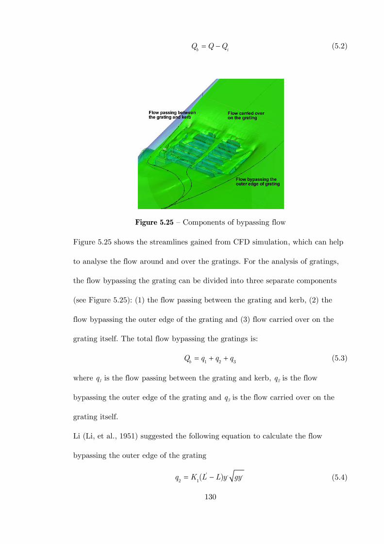
130
b iQ Q Q (5.2)
Figure 5.25 – Components of bypassing flow
Figure 5.25 shows the streamlines gained from CFD simulation, which can help
to analyse the flow around and over the gratings. For the analysis of gratings,
the flow bypassing the grating can be divided into three separate components
(see Figure 5.25): (1) the flow passing between the grating and kerb, (2) the
flow bypassing the outer edge of the grating and (3) flow carried over on the
grating itself. The total flow bypassing the gratings is:
1 2 3b
Q q q q (5.3)
where q1 is the flow passing between the grating and kerb, q2 is the flow
bypassing the outer edge of the grating and q3 is the flow carried over on the
grating itself.
Li (Li, et al., 1951) suggested the following equation to calculate the flow
bypassing the outer edge of the grating
' , ,2 1
( )q K L L y gy (5.4)
131
where K1 = 0.25, L’ is the length of grating required to capture the outer
portion of flow, L is the length of grating at outer edge, y’ is the depth at the
outer edge of grating. L’ is given by:
'
2 0,0
tanL g
Kv y
(5.5)
K2 = 1.2, tan 0
is the cross-slope of road surface, v0 is the average velocity at
the outer edge of grating.
These equations have been compared with CFD modelling results for
intermediate conditions. In the case of terminal and surcharging conditions the
term bypassing flow is difficult to interpret; therefore the results from these
were not included in the investigation. The investigation focussed on the
applicability and validity of the above equation. Different sloping conditions and
inflows were tested and it was found that the included parameters give sufficient
information to calculate the bypassing flow rate at the outer edge of the gully.
The evaluation of two constants K1 and K2 revealed that neither of them can be
considered as constant. The K1 parameter is a function of cross-slope described
by the following equation:
1
0
11.891exp 0.0067
tanK
(5.6)
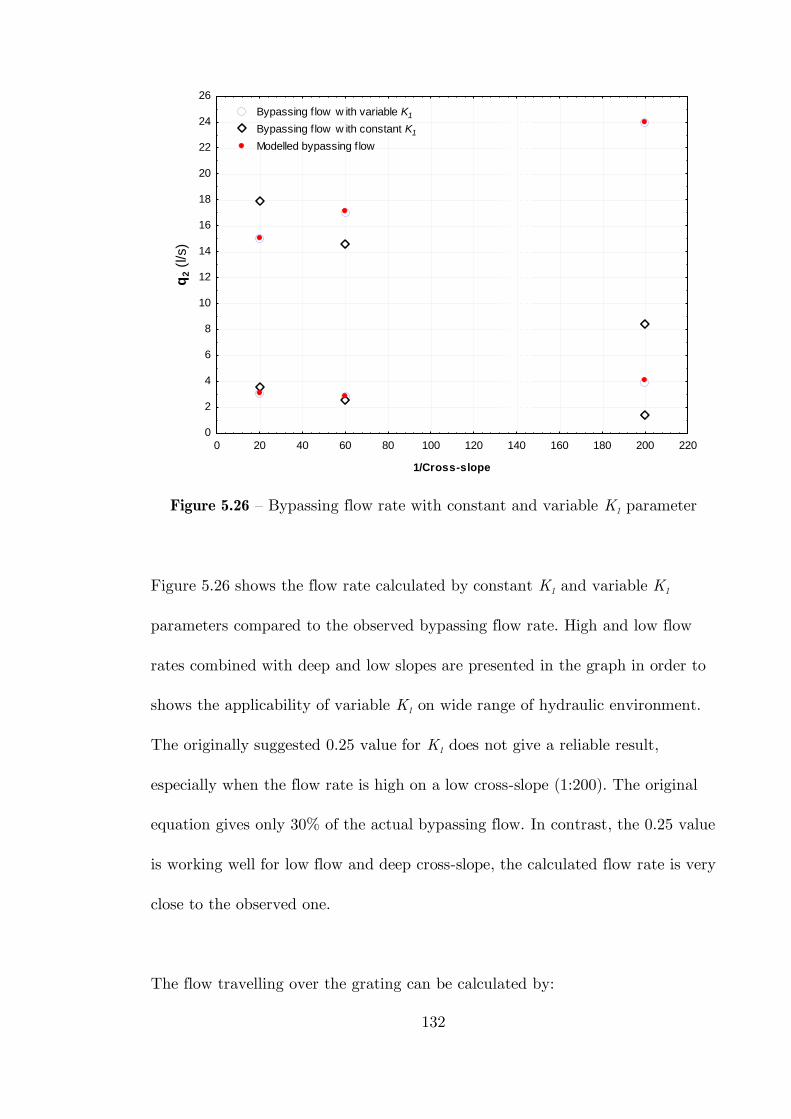
132
0 20 40 60 80 100 120 140 160 180 200 220
1/Cross-slope
0
2
4
6
8
10
12
14
16
18
20
22
24
26
q2 (
l/s)
Bypassing f low w ith variable K1
Bypassing f low w ith constant K1
Modelled bypassing f low
Figure 5.26 – Bypassing flow rate with constant and variable K1 parameter
Figure 5.26 shows the flow rate calculated by constant K1 and variable K1
parameters compared to the observed bypassing flow rate. High and low flow
rates combined with deep and low slopes are presented in the graph in order to
shows the applicability of variable K1 on wide range of hydraulic environment.
The originally suggested 0.25 value for K1 does not give a reliable result,
especially when the flow rate is high on a low cross-slope (1:200). The original
equation gives only 30% of the actual bypassing flow. In contrast, the 0.25 value
is working well for low flow and deep cross-slope, the calculated flow rate is very
close to the observed one.
The flow travelling over the grating can be calculated by:
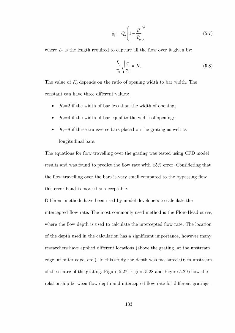
133
22
3 0 20
1L
q QL
(5.7)
where L0 is the length required to capture all the flow over it given by:
03
0 0
L gK
v y (5.8)
The value of K3 depends on the ratio of opening width to bar width. The
constant can have three different values:
K3=2 if the width of bar less than the width of opening;
K3=4 if the width of bar equal to the width of opening;
K3=8 if three transverse bars placed on the grating as well as
longitudinal bars.
The equations for flow travelling over the grating was tested using CFD model
results and was found to predict the flow rate with ±5% error. Considering that
the flow travelling over the bars is very small compared to the bypassing flow
this error band is more than acceptable.
Different methods have been used by model developers to calculate the
intercepted flow rate. The most commonly used method is the Flow-Head curve,
where the flow depth is used to calculate the intercepted flow rate. The location
of the depth used in the calculation has a significant importance, however many
researchers have applied different locations (above the grating, at the upstream
edge, at outer edge, etc.). In this study the depth was measured 0.6 m upstream
of the centre of the grating. Figure 5.27, Figure 5.28 and Figure 5.29 show the
relationship between flow depth and intercepted flow rate for different gratings.
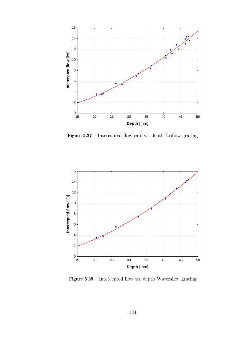
134
15 20 25 30 35 40 45 50
Depth [mm]
0
2
4
6
8
10
12
14
16
Inte
rcep
ted
flo
w [
l/s]
Figure 5.27 – Intercepted flow rate vs. depth Briflow grating
15 20 25 30 35 40 45 50
Depth [mm]
0
2
4
6
8
10
12
14
16
Inte
rcep
ted
flo
w [
l/s]
Figure 5.28 – Intercepted flow vs. depth Watershed grating
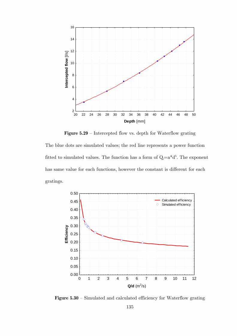
135
20 22 24 26 28 30 32 34 36 38 40 42 44 46 48 50
Depth [mm]
2
4
6
8
10
12
14
16
Inte
rcep
ted
flo
w [
l/s]
Figure 5.29 – Intercepted flow vs. depth for Waterflow grating
The blue dots are simulated values; the red line represents a power function
fitted to simulated values. The function has a form of Qi=a*db. The exponent
has same value for each functions, however the constant is different for each
gratings.
0 1 2 3 4 5 6 7 8 9 10 11 12
Q/d (m2/s)
0.00
0.05
0.10
0.15
0.20
0.25
0.30
0.35
0.40
0.45
0.50
Eff
icie
ncy
Calculated eff iciency
Simulated efficiency
Figure 5.30 – Simulated and calculated efficiency for Waterflow grating
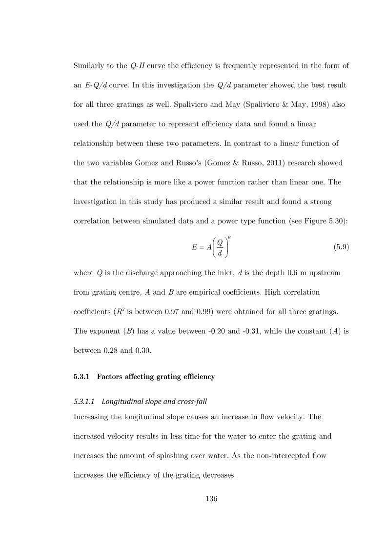
136
Similarly to the Q-H curve the efficiency is frequently represented in the form of
an E-Q/d curve. In this investigation the Q/d parameter showed the best result
for all three gratings as well. Spaliviero and May (Spaliviero & May, 1998) also
used the Q/d parameter to represent efficiency data and found a linear
relationship between these two parameters. In contrast to a linear function of
the two variables Gomez and Russo’s (Gomez & Russo, 2011) research showed
that the relationship is more like a power function rather than linear one. The
investigation in this study has produced a similar result and found a strong
correlation between simulated data and a power type function (see Figure 5.30):
B
QE A
d
(5.9)
where Q is the discharge approaching the inlet, d is the depth 0.6 m upstream
from grating centre, A and B are empirical coefficients. High correlation
coefficients (R2 is between 0.97 and 0.99) were obtained for all three gratings.
The exponent (B) has a value between -0.20 and -0.31, while the constant (A) is
between 0.28 and 0.30.
5.3.1 Factors affecting grating efficiency
5.3.1.1 Longitudinal slope and cross-fall
Increasing the longitudinal slope causes an increase in flow velocity. The
increased velocity results in less time for the water to enter the grating and
increases the amount of splashing over water. As the non-intercepted flow
increases the efficiency of the grating decreases.
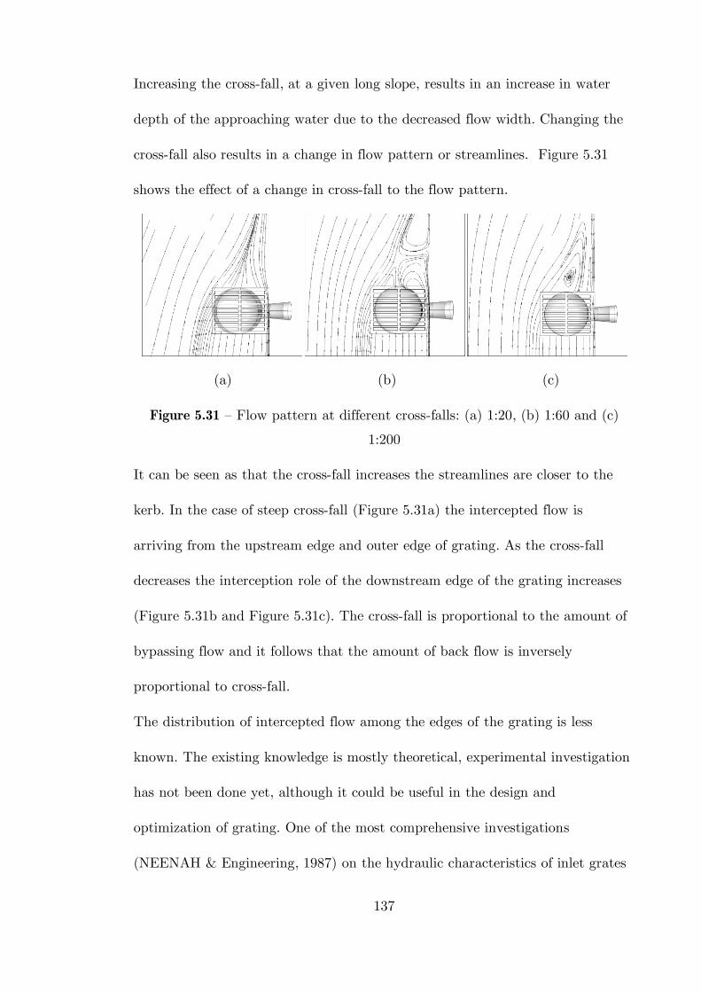
137
Increasing the cross-fall, at a given long slope, results in an increase in water
depth of the approaching water due to the decreased flow width. Changing the
cross-fall also results in a change in flow pattern or streamlines. Figure 5.31
shows the effect of a change in cross-fall to the flow pattern.
(a) (b) (c)
Figure 5.31 – Flow pattern at different cross-falls: (a) 1:20, (b) 1:60 and (c)
1:200
It can be seen as that the cross-fall increases the streamlines are closer to the
kerb. In the case of steep cross-fall (Figure 5.31a) the intercepted flow is
arriving from the upstream edge and outer edge of grating. As the cross-fall
decreases the interception role of the downstream edge of the grating increases
(Figure 5.31b and Figure 5.31c). The cross-fall is proportional to the amount of
bypassing flow and it follows that the amount of back flow is inversely
proportional to cross-fall.
The distribution of intercepted flow among the edges of the grating is less
known. The existing knowledge is mostly theoretical, experimental investigation
has not been done yet, although it could be useful in the design and
optimization of grating. One of the most comprehensive investigations
(NEENAH & Engineering, 1987) on the hydraulic characteristics of inlet grates
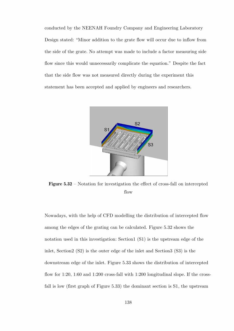
138
conducted by the NEENAH Foundry Company and Engineering Laboratory
Design stated: “Minor addition to the grate flow will occur due to inflow from
the side of the grate. No attempt was made to include a factor measuring side
flow since this would unnecessarily complicate the equation.” Despite the fact
that the side flow was not measured directly during the experiment this
statement has been accepted and applied by engineers and researchers.
Figure 5.32 – Notation for investigation the effect of cross-fall on intercepted
flow
Nowadays, with the help of CFD modelling the distribution of intercepted flow
among the edges of the grating can be calculated. Figure 5.32 shows the
notation used in this investigation: Section1 (S1) is the upstream edge of the
inlet, Section2 (S2) is the outer edge of the inlet and Section3 (S3) is the
downstream edge of the inlet. Figure 5.33 shows the distribution of intercepted
flow for 1:20, 1:60 and 1:200 cross-fall with 1:200 longitudinal slope. If the cross-
fall is low (first graph of Figure 5.33) the dominant section is S1, the upstream
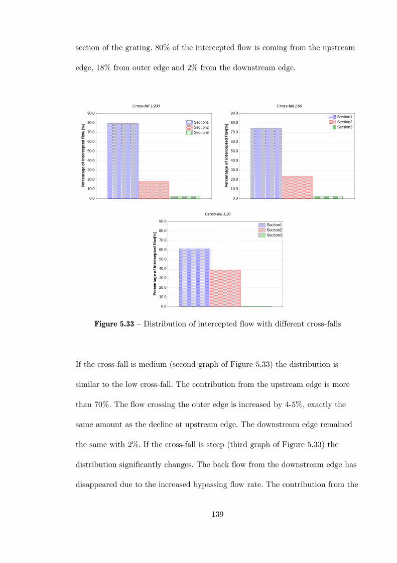
139
section of the grating. 80% of the intercepted flow is coming from the upstream
edge, 18% from outer edge and 2% from the downstream edge.
Cross-fall 1:200
0.0
10.0
20.0
30.0
40.0
50.0
60.0
70.0
80.0
90.0
Perc
en
tag
e o
f in
terc
ep
ted
flo
w [%
] Section1
Section2
Section3
Cross-fall 1:60
0.0
10.0
20.0
30.0
40.0
50.0
60.0
70.0
80.0
90.0
Perc
en
tag
e o
f in
terc
ep
ted
flo
w [%
]
Section1
Section2
Section3
Cross-fall 1:20
0.0
10.0
20.0
30.0
40.0
50.0
60.0
70.0
80.0
90.0
Perc
en
tag
e o
f in
terc
ep
ted
flo
w [%
]
Section1
Section2
Section3
Figure 5.33 – Distribution of intercepted flow with different cross-falls
If the cross-fall is medium (second graph of Figure 5.33) the distribution is
similar to the low cross-fall. The contribution from the upstream edge is more
than 70%. The flow crossing the outer edge is increased by 4-5%, exactly the
same amount as the decline at upstream edge. The downstream edge remained
the same with 2%. If the cross-fall is steep (third graph of Figure 5.33) the
distribution significantly changes. The back flow from the downstream edge has
disappeared due to the increased bypassing flow rate. The contribution from the
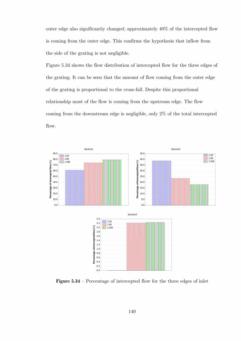
140
outer edge also significantly changed; approximately 40% of the intercepted flow
is coming from the outer edge. This confirms the hypothesis that inflow from
the side of the grating is not negligible.
Figure 5.34 shows the flow distribution of intercepted flow for the three edges of
the grating. It can be seen that the amount of flow coming from the outer edge
of the grating is proportional to the cross-fall. Despite this proportional
relationship most of the flow is coming from the upstream edge. The flow
coming from the downstream edge is negligible, only 2% of the total intercepted
flow.
Section1
0.0
10.0
20.0
30.0
40.0
50.0
60.0
70.0
80.0
90.0
Perc
en
tag
e o
f in
terc
ep
ted
flo
w [%
]
1:20
1:60
1:200
Section2
0.0
5.0
10.0
15.0
20.0
25.0
30.0
35.0
40.0
45.0
Perc
en
tag
e o
f in
terc
ep
ted
flo
w [%
]
1:20
1:60
1:200
Section3
0.0
0.2
0.4
0.6
0.8
1.0
1.2
1.4
1.6
1.8
2.0
2.2
2.4
Perc
en
tag
e o
f in
terc
ep
ted
flo
w [%
]
1:20
1:60
1:200
Figure 5.34 – Percentage of intercepted flow for the three edges of inlet
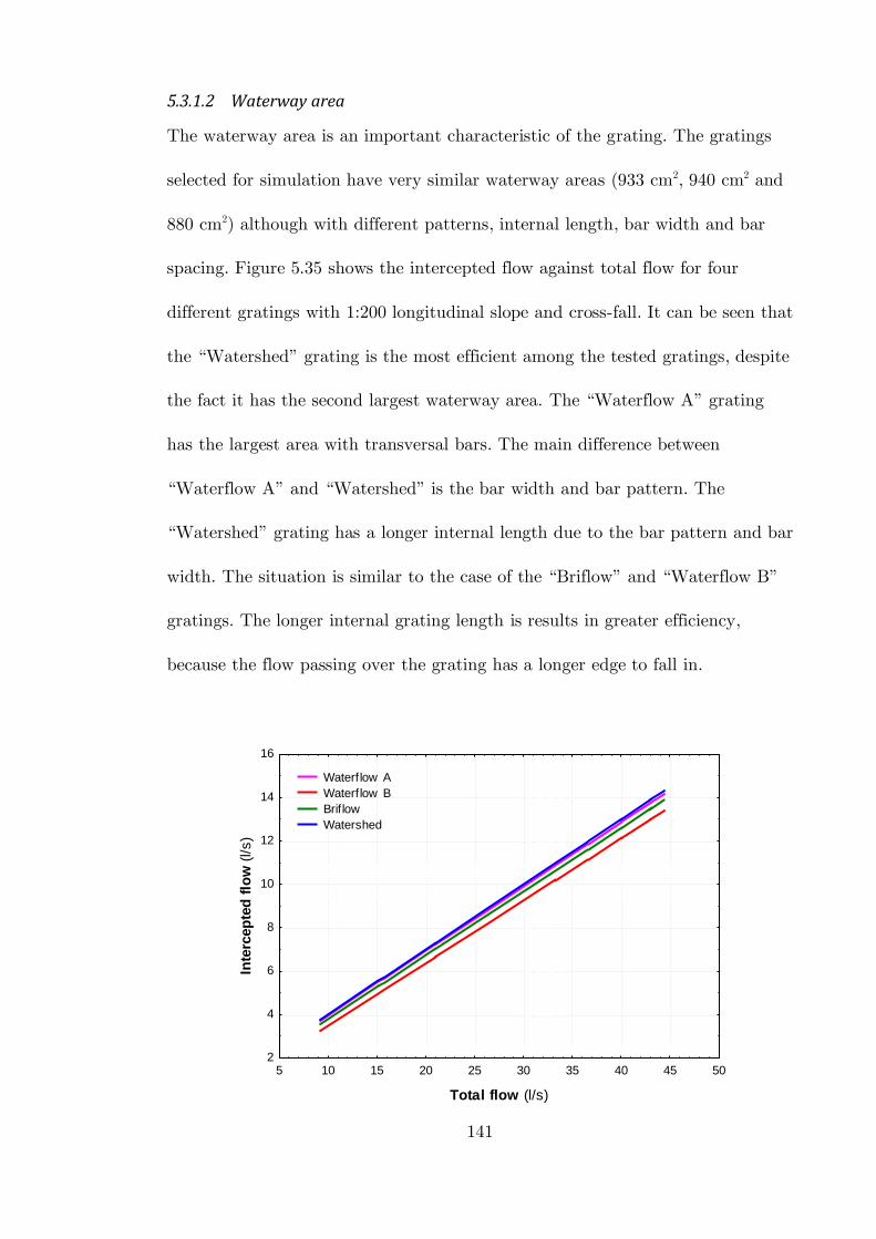
141
5.3.1.2 Waterway area
The waterway area is an important characteristic of the grating. The gratings
selected for simulation have very similar waterway areas (933 cm2, 940 cm2 and
880 cm2) although with different patterns, internal length, bar width and bar
spacing. Figure 5.35 shows the intercepted flow against total flow for four
different gratings with 1:200 longitudinal slope and cross-fall. It can be seen that
the “Watershed” grating is the most efficient among the tested gratings, despite
the fact it has the second largest waterway area. The “Waterflow A” grating
has the largest area with transversal bars. The main difference between
“Waterflow A” and “Watershed” is the bar width and bar pattern. The
“Watershed” grating has a longer internal length due to the bar pattern and bar
width. The situation is similar to the case of the “Briflow” and “Waterflow B”
gratings. The longer internal grating length is results in greater efficiency,
because the flow passing over the grating has a longer edge to fall in.
5 10 15 20 25 30 35 40 45 50
Total flow (l/s)
2
4
6
8
10
12
14
16
Inte
rcep
ted
flo
w (
l/s)
Waterf low A
Waterf low B
Brif low
Watershed
142
Figure 5.35 – Total flow vs. intercepted flow for different gratings
5.4 Surcharging conditions
Regarding the distinct stages and processes for the case of a surcharged drain
system the urban flooding simulation models are required to accurately describe
the hydraulic phenomena of a surcharged gully, particularly:
the transition from free surface flow to pressurized flow
the interaction between surface flow and pressurized flow
the rise of the water level above surface level
Numerous experiments have been undertaken worldwide in connection with
grate efficiency. All the experiments related to gratings/gullies are based on the
most frequent situation, when the flow direction is from the surface into the
gully. In this study surcharging conditions have also been investigated. This
type of flow condition is getting more attention nowadays from numerical
modellers; however it has not been studied experimentally before.
Figure 5.36 shows fifteen snapshots of the unsteady flow simulation following
sudden short-lived surcharging of the gully. The extent of the road surface and
the height of the cube are only a cropped portion of the computational domain
that extends further through the top and the three sides. The cube selected here
is just for the presentation of results. It can be seen that the simulation starts
with an empty domain. Initially the gully is empty and the road surface is dry.
143
Once the water starts entering the gully from the pipe connection underneath
(first row, second image), the water leaves the gully through the inlet grating in
a fashion that reflects the water pressure distribution within the gully.
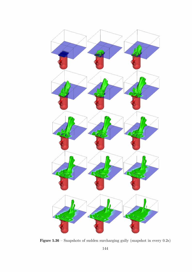
144
Figure 5.36 – Snapshots of sudden surcharging gully (snapshot in every 0.2s)
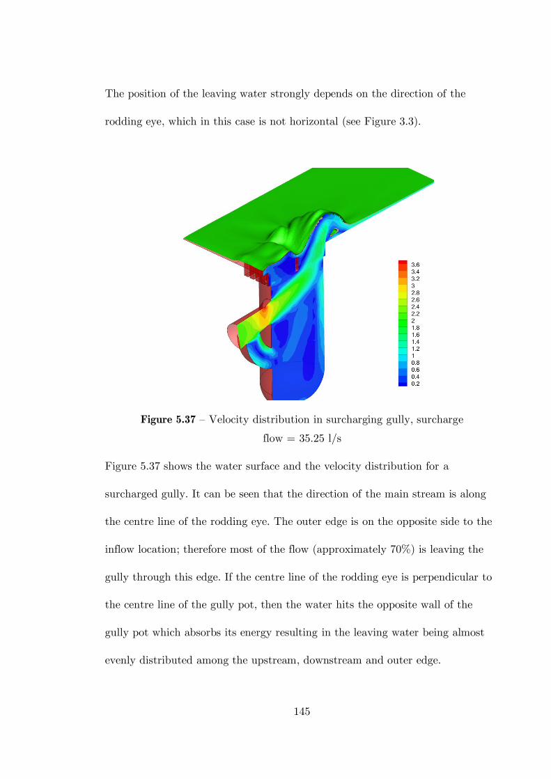
145
The position of the leaving water strongly depends on the direction of the
rodding eye, which in this case is not horizontal (see Figure 3.3).
Figure 5.37 – Velocity distribution in surcharging gully, surcharge
flow = 35.25 l/s
Figure 5.37 shows the water surface and the velocity distribution for a
surcharged gully. It can be seen that the direction of the main stream is along
the centre line of the rodding eye. The outer edge is on the opposite side to the
inflow location; therefore most of the flow (approximately 70%) is leaving the
gully through this edge. If the centre line of the rodding eye is perpendicular to
the centre line of the gully pot, then the water hits the opposite wall of the
gully pot which absorbs its energy resulting in the leaving water being almost
evenly distributed among the upstream, downstream and outer edge.
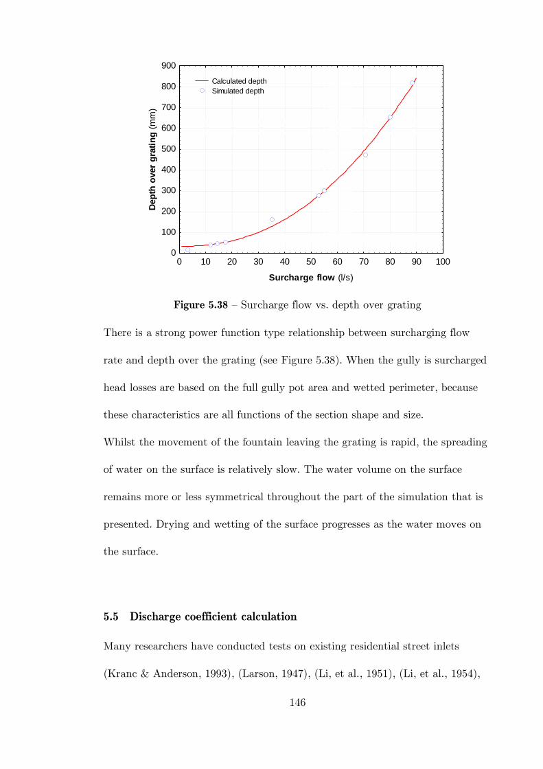
146
0 10 20 30 40 50 60 70 80 90 100
Surcharge flow (l/s)
0
100
200
300
400
500
600
700
800
900
Dep
th o
ver
gra
tin
g (
mm
)
Calculated depth
Simulated depth
Figure 5.38 – Surcharge flow vs. depth over grating
There is a strong power function type relationship between surcharging flow
rate and depth over the grating (see Figure 5.38). When the gully is surcharged
head losses are based on the full gully pot area and wetted perimeter, because
these characteristics are all functions of the section shape and size.
Whilst the movement of the fountain leaving the grating is rapid, the spreading
of water on the surface is relatively slow. The water volume on the surface
remains more or less symmetrical throughout the part of the simulation that is
presented. Drying and wetting of the surface progresses as the water moves on
the surface.
5.5 Discharge coefficient calculation
Many researchers have conducted tests on existing residential street inlets
(Kranc & Anderson, 1993), (Larson, 1947), (Li, et al., 1951), (Li, et al., 1954),
147
(McEnroe, et al., 1999), (Valentin & Russo, 2007). Their results are not
generally applicable unless similar conditions are applied. Even interpolation of
the existing results is believed to be difficult.
Flow over the grate represents a typical example of spatially varied flow with
decreasing discharge. Several authors have proposed equations for spatially
varied flow profiles relating the intercepted flow to the specific energy or flow
depth (Mostkow, 1957), (Noseda, 1956), (Subramanya & Senputa, 1981). These
studies considered only the frontal flow for the calculation of discharge
coefficient.
The inlet may operate like a weir when the water depth is shallow, or like an
orifice when it is submerged (Guo, 1997), (Guo, 2000a), (Guo, 2000b), (Guo,
2000c), (Mays, 2001). For a grate inlet that operates as a weir, the intercepted
flow is given by the following equation:
0120
32 2 21 1
0 0
0
12 2
2 1.5 2
h
hQ
i
v vQ dQ b g h dh b g h
g g
(5.10)
3/2 3/22 21 1
0
22
3 2 2i
v vQ gb h
g g
(5.11)
Introducing the discharge coefficient to incorporate the local losses:
3/2 3/22 21 1
1 0
22
3 2 2i d
v vQ C gb h
g g
(5.12)
In case of small velocity the
3/221
2
v
g
term is negligible or can be included in
the discharge coefficient, therefore:
148
3/21 1
22
3i dQ C gbH (5.13)
where Qi is the discharge intercepted by the inlet, Cd1, is the weir discharge
coefficient, which has a value between 0.6 - 0.7 (Butler & Davies, 2004), b is the
length of the inlet and H1 is the total head of water over the inlet. The key issue
is the location where H1 is measured (McEnroe, et al., 1999). The location of the
critical-flow section depends on the geometry of the surrounding area of the
inlet opening. Critical-flow does not necessarily occur at the perimeter of the
inlet opening. In some cases, the exact location H1 is uncertain and must be
estimated.
Rehbock found experimentally that:
1
10.611 0.08
305d
HC
W H (5.14)
The above equation neglects the viscous and surface tension effects, therefore is
only valid when the total head is not small. Based on Rehbock’s research many
investigators have confirmed the value of 0.611. Most design procedures assume
a constant value for the discharge coefficient regardless of the characteristics of
the flow. Experience has shown that the discharge coefficient is unlikely to be
invariant at all flow rates. Preliminary investigation shows that in contrast a
variable discharge coefficient can help to establish better design criteria for gully
inlets (Galambos, et al., 2009).
The intercepted discharge can be calculated using the kinetic energy coefficient
(), momentum coefficient () and the energy loss between the two sections
(hL):
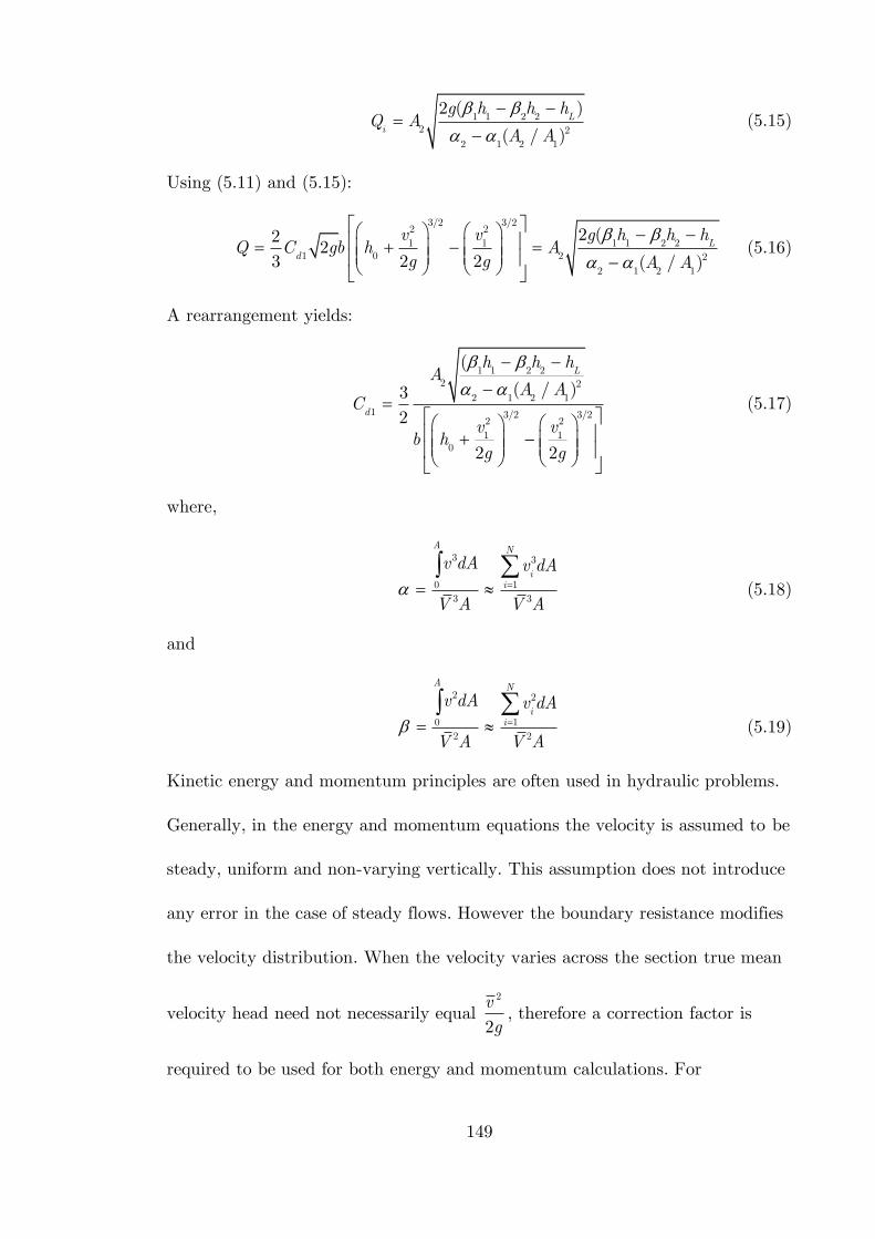
149
1 1 2 22 2
2 1 2 1
2 ( )
( / )L
i
g h h hQ A
A A
(5.15)
Using (5.11) and (5.15):
3/2 3/22 21 1 1 1 2 2
1 0 2 22 1 2 1
2 (22
3 2 2 ( / )L
d
v v g h h hQ C gb h A
g g A A
(5.16)
A rearrangement yields:
1 1 2 22 2
2 1 2 1
1 3/2 3/22 21 1
0
(
( / )3
2
2 2
L
d
h h hA
A AC
v vb h
g g
(5.17)
where,
3 3
0 13 3
A N
ii
v dA v dA
V A V A
(5.18)
and
2 2
0 12 2
A N
ii
v dA v dA
V A V A
(5.19)
Kinetic energy and momentum principles are often used in hydraulic problems.
Generally, in the energy and momentum equations the velocity is assumed to be
steady, uniform and non-varying vertically. This assumption does not introduce
any error in the case of steady flows. However the boundary resistance modifies
the velocity distribution. When the velocity varies across the section true mean
velocity head need not necessarily equal 2
2
v
g, therefore a correction factor is
required to be used for both energy and momentum calculations. For
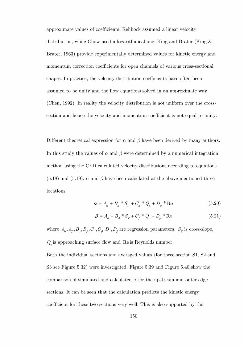
150
approximate values of coefficients, Rehbock assumed a linear velocity
distribution, while Chow used a logarithmical one. King and Brater (King &
Brater, 1963) provide experimentally determined values for kinetic energy and
momentum correction coefficients for open channels of various cross-sectional
shapes. In practice, the velocity distribution coefficients have often been
assumed to be unity and the flow equations solved in an approximate way
(Chen, 1992). In reality the velocity distribution is not uniform over the cross-
section and hence the velocity and momentum coefficient is not equal to unity.
Different theoretical expression for and have been derived by many authors.
In this study the values of and were determined by a numerical integration
method using the CFD calculated velocity distributions according to equations
(5.18) and (5.19). and have been calculated at the above mentioned three
locations.
* * * ReT u
A B S C Q D
(5.20)
* * * ReT u
A B S C Q D
(5.21)
where , , , , , , ,A A B B C C D D
are regression parameters, TS is cross-slope,
uQ is approaching surface flow and Re is Reynolds number.
Both the individual sections and averaged values (for three section S1, S2 and
S3 see Figure 5.32) were investigated. Figure 5.39 and Figure 5.40 show the
comparison of simulated and calculated for the upstream and outer edge
sections. It can be seen that the calculation predicts the kinetic energy
coefficient for these two sections very well. This is also supported by the
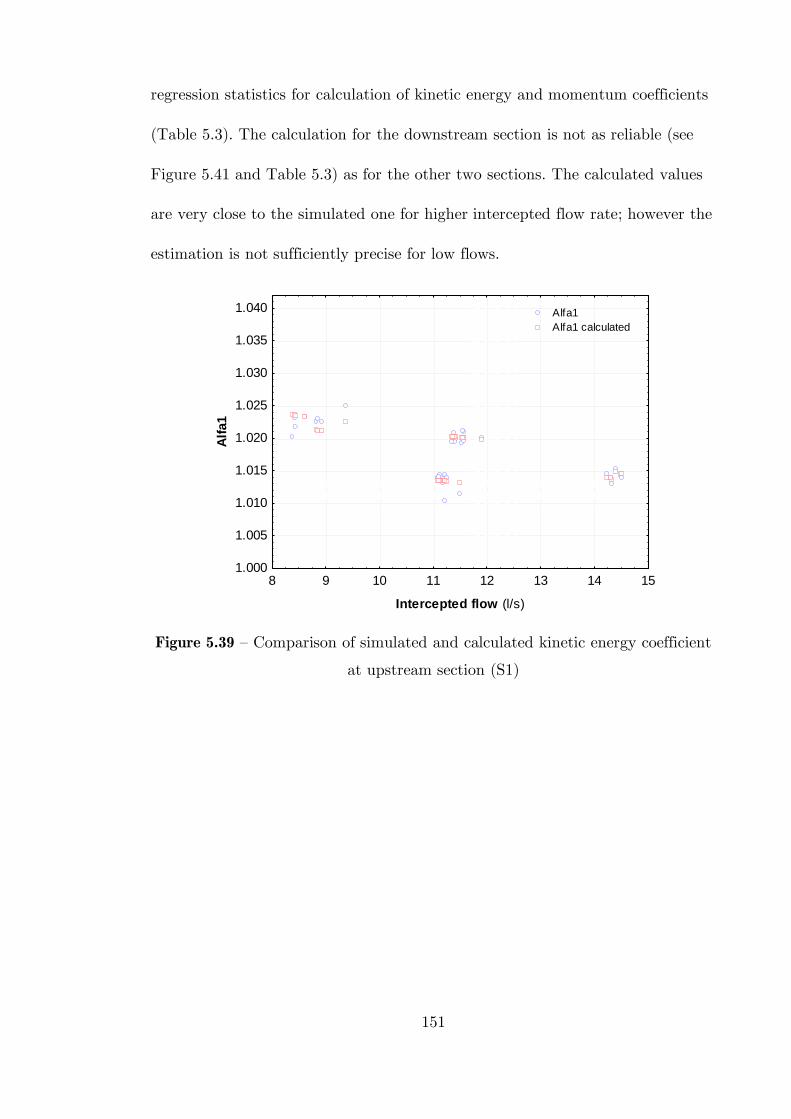
151
regression statistics for calculation of kinetic energy and momentum coefficients
(Table 5.3). The calculation for the downstream section is not as reliable (see
Figure 5.41 and Table 5.3) as for the other two sections. The calculated values
are very close to the simulated one for higher intercepted flow rate; however the
estimation is not sufficiently precise for low flows.
8 9 10 11 12 13 14 15
Intercepted flow (l/s)
1.000
1.005
1.010
1.015
1.020
1.025
1.030
1.035
1.040
Alf
a1
Alfa1
Alfa1 calculated
Figure 5.39 – Comparison of simulated and calculated kinetic energy coefficient
at upstream section (S1)
152
8 9 10 11 12 13 14 15
Intercepted flow (l/s)
1.000
1.005
1.010
1.015
1.020
1.025
1.030
1.035
1.040
Alf
a2
Alfa2
Alfa2 calculated
Figure 5.40 – Comparison of simulated and calculated kinetic energy coefficient
at outer edge section (S2)
8 9 10 11 12 13 14 15
Intercepted flow (l/s)
1.000
1.200
1.400
1.600
1.800
2.000
2.200
2.400
2.600
Alf
a3
Alfa3
Alfa3 calculated
Figure 5.41 – Comparison of simulated and calculated kinetic energy coefficient
at downstream section (S3)
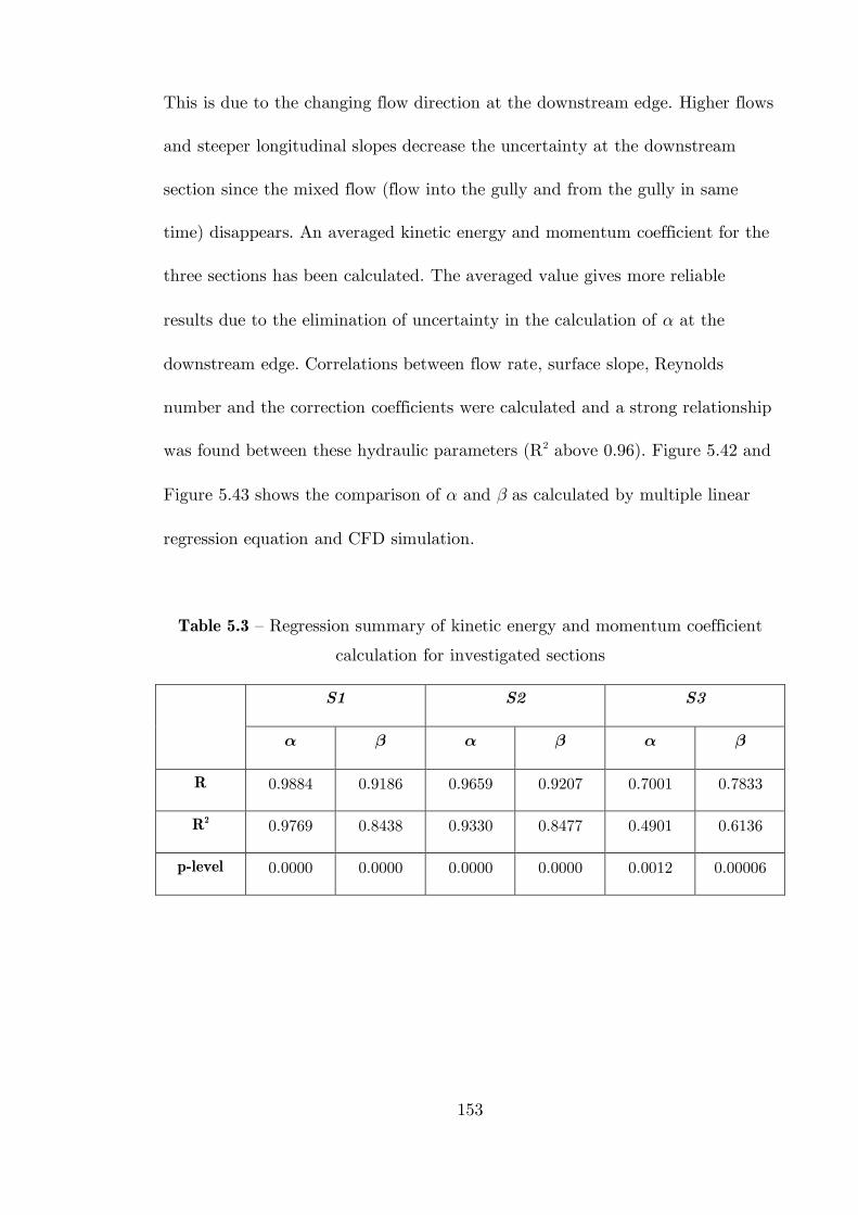
153
This is due to the changing flow direction at the downstream edge. Higher flows
and steeper longitudinal slopes decrease the uncertainty at the downstream
section since the mixed flow (flow into the gully and from the gully in same
time) disappears. An averaged kinetic energy and momentum coefficient for the
three sections has been calculated. The averaged value gives more reliable
results due to the elimination of uncertainty in the calculation of at the
downstream edge. Correlations between flow rate, surface slope, Reynolds
number and the correction coefficients were calculated and a strong relationship
was found between these hydraulic parameters (R2 above 0.96). Figure 5.42 and
Figure 5.43 shows the comparison of and as calculated by multiple linear
regression equation and CFD simulation.
Table 5.3 – Regression summary of kinetic energy and momentum coefficient
calculation for investigated sections
S1 S2 S3
R 0.9884 0.9186 0.9659 0.9207 0.7001 0.7833
R2 0.9769 0.8438 0.9330 0.8477 0.4901 0.6136
p-level 0.0000 0.0000 0.0000 0.0000 0.0012 0.00006
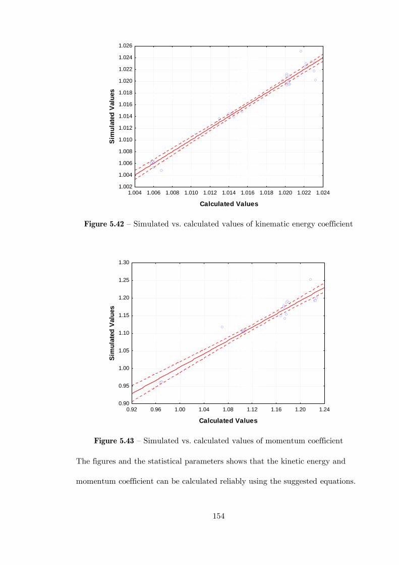
154
1.004 1.006 1.008 1.010 1.012 1.014 1.016 1.018 1.020 1.022 1.024
Calculated Values
1.002
1.004
1.006
1.008
1.010
1.012
1.014
1.016
1.018
1.020
1.022
1.024
1.026
Sim
ula
ted
Valu
es
Figure 5.42 – Simulated vs. calculated values of kinematic energy coefficient
0.92 0.96 1.00 1.04 1.08 1.12 1.16 1.20 1.24
Calculated Values
0.90
0.95
1.00
1.05
1.10
1.15
1.20
1.25
1.30
Sim
ula
ted
Valu
es
Figure 5.43 – Simulated vs. calculated values of momentum coefficient
The figures and the statistical parameters shows that the kinetic energy and
momentum coefficient can be calculated reliably using the suggested equations.
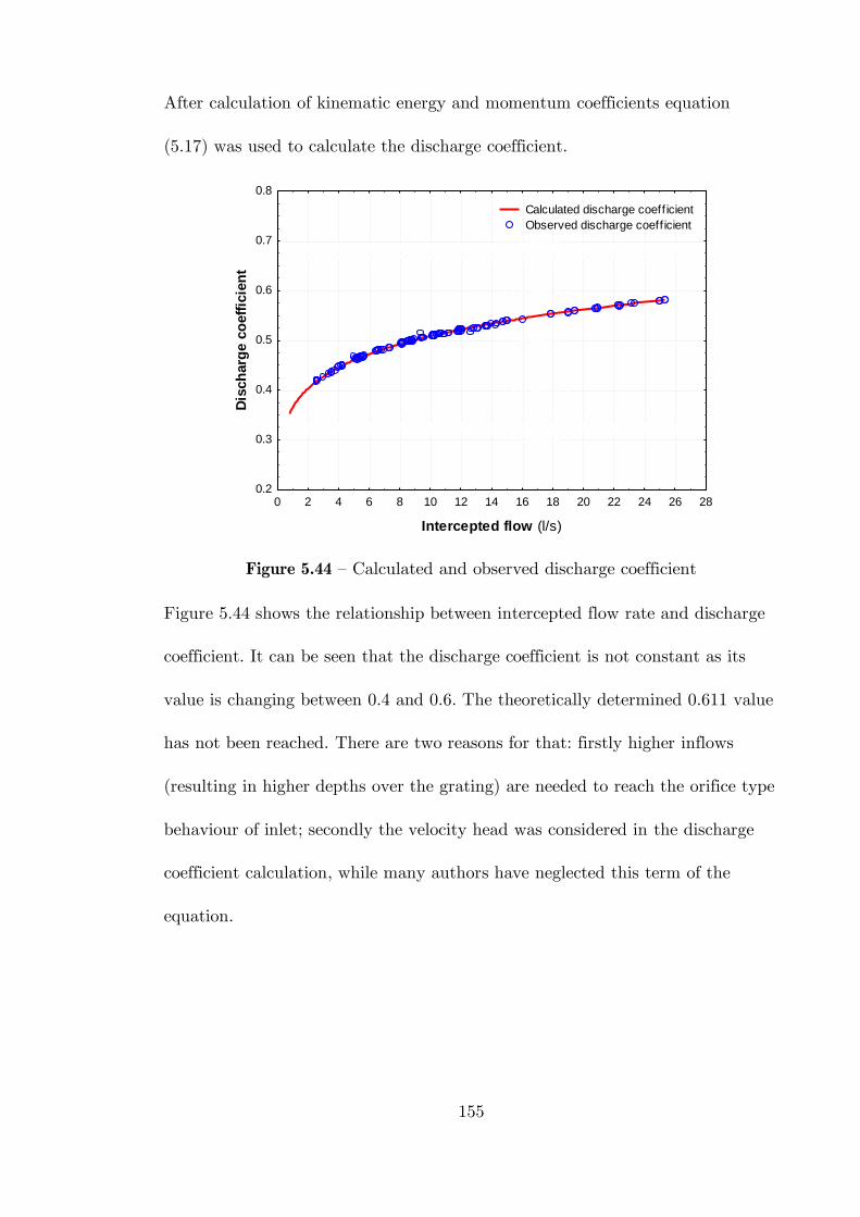
155
After calculation of kinematic energy and momentum coefficients equation
(5.17) was used to calculate the discharge coefficient.
0 2 4 6 8 10 12 14 16 18 20 22 24 26 28
Intercepted flow (l/s)
0.2
0.3
0.4
0.5
0.6
0.7
0.8
Dis
ch
arg
e c
oeff
icie
nt
Calculated discharge coeff icient
Observed discharge coeff icient
Figure 5.44 – Calculated and observed discharge coefficient
Figure 5.44 shows the relationship between intercepted flow rate and discharge
coefficient. It can be seen that the discharge coefficient is not constant as its
value is changing between 0.4 and 0.6. The theoretically determined 0.611 value
has not been reached. There are two reasons for that: firstly higher inflows
(resulting in higher depths over the grating) are needed to reach the orifice type
behaviour of inlet; secondly the velocity head was considered in the discharge
coefficient calculation, while many authors have neglected this term of the
equation.
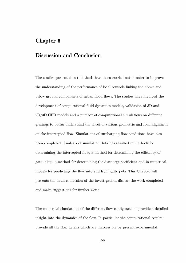
156
Chapter 6
Discussion and Conclusion
The studies presented in this thesis have been carried out in order to improve
the understanding of the performance of local controls linking the above and
below ground components of urban flood flows. The studies have involved the
development of computational fluid dynamics models, validation of 3D and
2D/3D CFD models and a number of computational simulations on different
gratings to better understand the effect of various geometric and road alignment
on the intercepted flow. Simulations of surcharging flow conditions have also
been completed. Analysis of simulation data has resulted in methods for
determining the intercepted flow, a method for determining the efficiency of
gate inlets, a method for determining the discharge coefficient and in numerical
models for predicting the flow into and from gully pots. This Chapter will
presents the main conclusion of the investigation, discuss the work completed
and make suggestions for further work.
The numerical simulations of the different flow configurations provide a detailed
insight into the dynamics of the flow. In particular the computational results
provide all the flow details which are inaccessible by present experimental
157
techniques. They are used to prove the theoretical assumptions and yield the
required information for analytical modelling.
This study shows that an advanced CFD model can be used to evaluate inlet
performance due to different inlet geometries, longitudinal slope and cross slope
instead of conducting large numbers of expensive laboratory tests.
The capabilities of interface capturing procedure based on Volume-of-Fluid
method were assessed. The three dimensional computational model for two-
phase flow with interface capturing was extended with two dimensional model
and a link between the two computational domains. A special type of boundary
has been used to connect the 2D and 3D domains. This switches velocity and
pressure between fixed value and zero gradient depending on the direction of
flow. The nesting has a significant positive effect on simulation time. Special
attention has been made to mesh generation because the design and
construction of a quality mesh is crucial to the success of the CFD analysis. The
advantages and disadvantages of different mesh types have been assessed.
The models were validated by comparing the computational results with
experimental results.
In Chapter 5 the distribution of intercepted flow among the edges of the grating
has been investigated and it was shown that the contribution to intercepted
flow from the outer edge of grating can be significant in certain conditions. This
result apparently contradicts the observations that led NEENAH Foundry
158
Company and Engineering Laboratory Design to suggest that a negligible
amount of the intercepted flow arrives through the outer edge of the inlet. It
was shown that the amount of flow arriving from the outer edge of the grating
is proportional to the cross-fall.
An improvement to the bypassing flow calculation was suggested. Different
sloping conditions and inflows were tested and it was found that the included
parameters give sufficient information to calculate the bypassing flow rate. It
was shown that the empirical constant K1 is a function of cross-slope.
Intercepted flow – depth functions were identified for three commonly used
gratings. The regression analysis showed that the suggested equation can
reliably predict the intercepted flow rate. Similarly to Q-H curve the Efficiency-
Q/d curve was identified for the selected gratings.
Factors affecting grating efficiency have been investigated and yielded the
following observations and conclusions. Under certain conditions a larger
opening does not increase the effectiveness of a grating. This is because the
dimensions and bar pattern influence the way that the flow is captured.
Streamlines for different cross-fall scenarios were calculated and its effect on
efficiency was investigated.
A regression relationship that related the approaching flow and water depth to
inlet efficiency was identified.
The surcharging condition has been investigated to better understand the
interaction between the surface and subsurface elements of urban flood models.
A surcharge flow – depth function was identified as part of the investigation.
159
A realistic value for the street inlet can be calculated for certain flow conditions.
The assumption that the discharge coefficient is constant and equal to 0.6 was
proven to be wrong. A methodology for calculation of variable discharge
coefficient was established.
Suggestions for further work
Numerical simulation of floods is very complex and interesting hydraulic
problem. However, modelling is not only the objective but has serious ambitions
in terms of reducing the flood consequences. All these problems are always
further intensified by the combined effect of climate change and population
growth. Below are listed some of the problems which could be in the focus of
research in the future.
Although the numerical models were validated successfully against water
depths data collected during experimental tests, it would be interesting
to make a further comparison of the velocity distribution at selected
sections.
Parasitic currents are attributed to the inaccurate determination of free
surface and this is commonly encountered in VOF method based
simulations. It has been found that the VOF method remain one of the
most suitable methods for interface capturing in the framework of finite
volume method without explicit free surface reconstruction. However,
possibilities for improvement of interface sharpness with level set method
should be further analysed.

160
The computational 2D/3D link should be further extended to include
tetrahedral type linkage, which would increase the flexibility and
probably the effectiveness of the existing link.
The gully inlets frequently blocked by debris. Proper design and
management of these systems are essential to minimize flood damage and
disruptions in urban areas during storm events. The effect of blockage
has not been tested either experimentally or numerically. The CFD
modelling of debris blockage and its effect on inlet efficiency would
generate valuable knowledge both for designers and modellers as well.
Similarly to debris, the sedimentation of gully pots and connected pipe
system is frequently causing flood damage and disruption of urban
transport. The developed multi-phase model can easily be extended into
three phase model (water, air and sediment), which would provide a
powerful tool to investigate the sedimentation process and could help to
develop sediment management methods.
The gratings has a significant effect on inlet efficiency. The applied CFD
model could help to develop hidrodynamically optimal gratings.
161
References
Almedeij, A. O.,Houghtalen, R. J. (2003): Urban hydrology: hydraulics and
storm water quality. John Wiley & Son.
Andersson, B. et al. (2012): Computational Fluid Dynamics for Engineers.
Cambridge: Cambridge University Press.
ANSYS (2006): Fluent 6.3 User Guide.
Aris, R. (1989): Vectors, tensors and the basic equations of fluid mechanics.
Dover Publications.
Aulisa, E., Manservisi, S., Scardovelli, R. (2003): A mixed markers and volume-
of-fluid method for the reconstruction and advection of interfaces in two-
phase and free boundary flows. Journal of Computational Physics, Volume
188, pp. 611-639.
Aulisa, E., Manservisi, S., Scardovelli, R. (2004): A geometrical area-preserving
volume-of-fluid advection method. Journal of Computational Physics,
Volume 192, pp. 355-364.
Balmforth, D., Digman, C., Kellagher, R., Butler, D. (2006): Design for
exceedence in urban drainage - good practice
Bates, P. D., Lane, S. N., Ferguson, R. I. (2005): Computational Fluid
Dynamics - Applications in Environmental Hydraulics.John Wiley & Sons
Ltd..
Blazek, J. (2001): Computational Fluid Dynamics: Principles and Applications.
Oxford: Elsevier.
Borghei, S. M., Jalili, M. R., Ghodsian, M. (1999): Discharge coefficient for
sharp-crested side weir in subcritical flow. Journal of Hydraulic
Engineering, 125(10), pp. 1051-1056.
Bourchard, M. G., Towsend, R. D. (1984): Laboratory tests on the influence of
grating pattern on street inlet hydraulics. Montreal, pp. 685-698.
162
Brackbill, J. U., Kothe, D. B., Zemach, C. (1992): A continuum method for
modelling surface tension. Journal of Computational Physics, Volume 100,
pp. 335-354.
Brennan, D. (2001): The numerical simulation of two-phase flows in settling
tanks, PhD thesis
Brown, S. A., Stein, S. M., Warner, J. C. (2001): Urban Drainage Design
Manual - Hydraulic Engineering Circular 22
Burgi, P. H., Gober, D. E. (1978): Hydraulic and Safety Characeristics of
Selected Grate Inlets. Transportation Research Record, Issue No. 685, pp.
29-31.
Butler, D., Davies, J. W. (2004): Urban Drainage. New York: Spon Press.
Buxton, A., Tait, S., Stovin, V., Saul, A. (2002). Developments in a
methodology for the design of engineered invert traps in combined sewer
systems. Water Science and Technology, 45(7), pp. 133-142.
Chen, C. L. (1992): Momntum and Energy Coefficient Based on Power-Law
Velocity Profile. ASCE Journal of Hydraulic Engineering, pp. 118 (11)
1571-1584.
Chow, V. T., 1959. Open channel hydraulics. New York: McGraw-Hill.
Croce, R., Griebel, M., Schweitzer, M. A. (2004): A Parallel Level-Set Approach
for Two-Phase Flow Problems with Surface Tension in Three Space
Dimensions
Cullivan, J. C., Williams, R. A., Dyakowski, T., Cross, C. R. (2004): New
understanding of a hydrocyclone field and separation mechanism from
computational fluid dynamics. Mineral Engineering, Volume 17, pp. 651-
660.
Datei, C. (1966): Remarks on the effects of surface tension on the shape of fluid
jets. Bressanone, NATO Advanced Study Institute.
163
De Martino, G. Ragone, A. (1979): L'influenza della viscosita e della tensione
superficiale sull'efflusso da lucci. Nouva Serie, Volume XXVIII.
Despotovic, J., Tomanovic, A., Batinic, B. (1990): Hydraulic explanation and
modelling of the capacity of urban storm drainage gutter pavment grate
inlets. Osaka, Japan, pp. 18-23.
Djordjevic, S. (2009): 1D, 2D and 3D modelling of urban flooding. Proceedings
of the 8th International Conference on Urban Drainage Modelling, Tokyo,
Japane
El-Kashab, A., Smith, K. V. H. (1976): Experimental investigation of flow over
side weirs. Journal of Hydraulic Engineering, 102(9), pp. 1255-1268.
Enright, D., Fedkiw, R., Ferziger, J., Mitchell, I. (2002): A hybrid particle level
set method for improved interface capturing. Journal of Computational
Physics, Volume 183, pp. 83-116.
ERCOFTAC (2000): Best Practice Guidlines for Industrial Computational
Fluid Dynamics of Single-Phase Flows, Lausanne
Evans, E. P., Ashley, R., Hall, J. W., Pennin-Rowsell, E. C., Saul, A., Sayers,
P. B., Thorne, C. R., Watkinson, A. (2004a): Foresight Flood and Coastal
Defence Project: Scientific Summary Vol. I, Future Risks and their drivers,
London, Office of Science and Technology.
Evans, E. P. , Ashley, R., Hall, J. W., Pennin-Rowsell, E. C., Saul, A., Sayers,
P. B., Thorne, C. R., Watkinson, A. (2004b): A Foresight Flood and
Coastal Defence Project: Scientific Summary: Volume 2, Managing future
risks, London, Office of Science and Technology.
Fach, S., Sitzenfrei, R., Rauch, W.(2009): Determining the spill flow discharge
of combined sewer overflows using rating curves based on computational
fluid dynamics instead of the standard weir equation. Water Science &
Technology, 60(12), pp. 3035-3043.
Fang, X., Jiang, S., Alam, S. R. (201): Numerical simulation of efficiency of
curb-opening inlets. Journal of Hydraulic Engineering, 136(1), pp. 62-66.
164
Ferziger, J. H., Peric, M. (1996): Computational methods for fluid dynamics.
Springer.
Galambos, I., Djordjevic, S., Tabor, G. (2009): FRMRC2 WP3.7 Improved
understanding of interaction between surface and underground drainage
systems, Progress Report, University of Exeter.
Gavis, J. (1964): Contribution of surface tension to expansion and contraction
of capillary jets. The Physics of Fluids.
Ghetti, A. (1966): Effects of surface tension on the shape of liquid jets.
Bressanone, NATO Advanced Study Institute.
Gomez, M., Russo, B. (2011): Methodology to estimate hydraulic efficiency of
drain inlets. Water Management, 164(WM2), pp. 81-90.
Guo, J. C. (1997): Street Hydraulics and Inlet Sizing, Littleton, Colorado:
Water Resources Publication.
Guo, J. C. (2000a): Design of grate inlets with clogging factor. Advances in
Environmental Research, pp. 4, 181-186.
Guo, J. C. (2000b): Street Storm Water Conveyance Capacity. ASCE Journal
of Irrigation and Drainage Engineering, pp. Vol. 126, No. 2.
Guo, J. C. (2000c): Street Storm Water Storage Capacity. Journal of
Environmental Research, pp. Vol. 27, No. 6.
Hager, W. H. (1987.):Lateral outflow over side weirs. 113(4), pp. 491-504.
Hansen, G. A., Douglass, R. W., Zardecki, A. (2005): Mesh enhancement.
London, Imperial College Press.
Harvie, D. J. E., Fletcher, D. F. (2000): A new volume of fluid advection
algorithm: the stream scheme. Journal of Computational Physics, Volume
162, pp. 1-32.
165
Harvie, D. J. E., Fletcher, D. F. (2001): A new volume of fluid advection
algorithm: The defined donating region scheme. International Journal for
Numerical Methods in Fluids, Volume 35, pp. 151-172.
Hill, D. P. (1998): The computer simulation of dispersed two-phase flows, PhD
thesis
Hirsch, C. (2007): Numerical Computation of Internal and External Flows.
Oxford: Elsevier.
Hirt, C. W., Nichols, B. D. (1981): Volume of fluid (VOF) method for the
dynamics of free boundaries. Journal of Computational Physics, Volume
39, pp. 201-225.
Honar, T., Keshavarzi, A. (2008): Effect of rounded-edge entrance on discharge
coefficient of side weir in rectangular channels. Irrigation and
drainage.Wiley Interscience
Huang, J. C., Weber, L. J., Lai, Y. G. (2002): Three dimensioanl numerical
study of flows in open channel junctions. Journal of Hydraulic
Engineering, 128(3), pp. 268-280.
Ismail, M., Nikraz, H. (2008): Experimental and Numerical Modeling of
VersaTrap Type G. Agricultural Engineering International, December,
Volume X..
Issa, R. I. (1986): Solution of the implicit discretized fluid flow equations by
operator-splitting. Journal of Computational Physics, Volume 62, pp. 40-
65.
Jarman, D. S., Faram, M. G., Butler, D., Tabor, G., Stovin, V. R., Burt, D.,
Thorp, E. (2008): Computational fluid dynamics as a tool for urban
drainage system analysis: A review of applications and best practice.
Proceedings of 11th International Conference on Urban Drainage,
Edinburgh, Scotland
Jasak, H. (1996). Error analysis and estimation for the finite volume method
with application to fluid flows, PhD thesis
166
Jiang, G. S., Peng, D. (2000): Weighted ENO Schemes for Hamilton-Jacobi
Equations. Journal of Scientific Computing, Issue 21, pp. 21-26.
John Hopkins University (1956): The design of storm-water inlets, Report of the
Storm Drainage Research Committe, Baltimore
Johnson, M. C. (2000): Discharge coefficient analysis for flat-topped and sharp-
crested weir. Irrigation Science, Volume 19, pp. 133-137.
Kindsvater, C. E., Carter, R. W. (1957): Discharge characteristics of rectangular
thin-plate weirs. Proceedings, December.Volume HY6.
King, H. W., Brater, E. F. (1963): Handbook of Hydraulics. New York:
McGraw-Hill.
Kranc, S. C., Anderson, M. W. (1993): Investigation Discharge through Grated
Inlets, Technical Report, University of South Florida.
Lafaurie, B., Nardone, C., Scardovelli, R., Zaleski, S., Zanetti, G. (1994):
Modelling merging and fragmentation in muliphase flows with SURFER.
Journal of Computational Physics, Volume 113, pp. 134-147.
Larson, C. L. (1947): Investigation of Flow Through Standard and Experimental
Grate Inlets for Street Gutters, Project Report, St. Antony Falls Hydraulic
Laboratory University of Minesota.
Leandro, J., Chen, A., Savic, D. A. (2009): Comparison of 1D/1D and 1D/2D
coupled (sewer/surface) hydraulic models for urban flood simulation.
Journal of Hydraulic Engineering ASCE, 135(6), pp. 495-504.
Leonard, B. P. (1991): The ULTIMATE conservative difference scheme applied
to unsteady one-dimensional advection. Computational Methods in Applied
Mechanics and Engineering, Volume 19, pp. 17-74.
Linquist, E. (1929): Precise weir measurement. Transaction, Volume 93.
Li, W. H., Geyer, J. C., Benton, G. S. (1951): Hydraulic Behaviour of Storm-
Water Inlets: I. Flow into Gutter Inlets in straight Gutter without
Depression. Sewage and Industrial Wastes, 23(1), pp. 34-46.
167
Li, W. H., Goodel, B. C., Geyer, J. C. (1954): Hydraulic Behavior of Storm-
Water Inlets: IV. Flow into Depressed Combination Inlets. Sewage and
Industrial Wastes, 26(8), pp. 967-975.
Lopez, J., Hernandez, J., Gomez, P., Faura, F. (2004): A volume of fluid
method based on multidimensional advection and spline interface
reconstruction. Journal of Computational Physics, Issue 195, pp. 718-742.
Mangani, L. (2008): Development and validation of an object oriented CFD
solver for heat transfer and combustion modeling in turbomachinery
applications, PhD thesis
MARNET-CFD, (1999): Best practice guidlines for marine application of
computational fluid dynamics,Project Report
Martino, G. D., Ragone, A. (1984): Effects of viscosity and surface tension on
slot weir flow. Journal of Hydraulic Research, 22(5), pp. 327-341.
Matthew, G. D. (1963): On the influence of curvature, surface tension and
viscosity on flow over round-crested weirs. Proceedings of the Institute of
Civil Engineering, ASCE, pp. 511-524.
Mays, L. R. (2001): Water Resources Engineering. New York: John Wiley &
Son.
McEnroe, B. M., Wade, R. P., Smith, A. K. (1999): Hydraulic performance of
curb and gutter inlets, Technical Report, Department of Civil and
Environmental Engineering University of Kansas
Menter, F. R. (1992): Assessment of higher order turbulence models for complex
two- and three-dimensional flowfields, Project Report, NASA-TM-103944,
National Aeronautics and Space Administration (NASA).
Menter, F. R. (2002): CFD Best Practice Guidlines for CFD Code Validation
for Reactor Safety Applications, Technical Report, FIKS-CT-2001-00154,
ECORA.
168
Mignot, E. Bonkadari, H., Knothe, P., Lipene Kouyi, G., Bessette, A., Riviere,
N., Bertrand-Krajewski, J. L., (2012): Experiments and 3D simulations of
flow structures in junctions and their influence on location of flow meters.
Water Science and Technology.
Mostkow, M. A. (1957): A theoretical study of bottom type water intakes. La
Houille Blanche, 4(12), pp. 570-580.
NEENAH Foundry Company, Engineering Laboratory Design (1987): Inlet
grate capacities for gutter flow and ponded water, Research Report
Noh, W. F., Woodward, P. (1976): SLIC (Simple Line Interface Calculations).
Lecture Notes in Physics, Volume 59, pp. 330-340.
Noseda, G. (1956): Correnti permanenti con portata progressivamente
decrescente, defluenti su griglie di fondo. L'Energia Electrica, 33(6), pp.
565-584.
OpenCFD (2008):OpenFOAM, The Open Source CFD Toolbox, User Guide
Osher, S. J., Sethian, J. (1988): Fronts Propagating with Curvature Dependent
Speed: Algorithms Based on Hamilton-Jacobi Formulations. Journal of
Computational Physics, Issue 79, pp. 12-49.
Osher, S., Sethian, J. A. (1988): Fronts propagating with curvature dependent
speed: Algorithms based on Hamilton-Jacobi formulations. Journal of
Computational Physics, Issue 79, pp. 12-49.
Pan, D., Chang, C. H. (2000): The capturing of free surfaces in incompressible
multi-fluid flows. International Journal of Numerical Methods in Fluids,
Volume 33, pp. 203-222.
Pantakar, S. V. (1980): Numerical heat transfer and fluid flow, Hemisphere
Publishing Corporation.
Peric, M. (1985): A finite volume method for the prediction of three-dimensional
flow in complex ducts, PhD thesis.
169
Pilliod, J. E., Pucket, E. G. (2004): Second-order accurate volume-of-fluid
algorithms for tracking material interfaces. Journal of Computational
Physics, Issue 199, pp. 465-502.
Pointwise (2008): Pointwise User Manual
Ranga Raju, K. G., Prasad, B., Gupta, S. K. (1979): Side weir in rectangular
channel. Journal of Hydraulic Division, 105(5), pp. 547-554.
Rehbock, T. (1929): Hydraulic laboratory practice. New York: American Society
of Mechanical Engineers
Renardy, Y., Renardy, M. (2002): PROST : A Parabolic Reconstruction of
Surface Tension for the Volume-Of-Fluid Method. Journal of
Computational Physics, Volume 183, pp. 400-421.
Rider, W. J., Kothe, D. B. (1998): Reconstructing volume tracking. Journal of
Computational Physics, Volume 141, pp. 112-152.
Rudman, M. (1997): Volume-tracking methods for interfacial flow calculations.
International Journal for Numerical Methods in Fluids, Volume 24, pp.
671-691.
Rusche, H. (2002): Computational Fluid Dynamics of dispersed two-phase flows
at high phase fractions, PhD thesis
Russo, B., Gomez, M., Martinez, P., Sanchez, H. (2005): Methodology to study
the surface runoff in urban streets and the design inlet systems.
Application in a real case study. Proceedings of the 10th International
Conference on Urban Drainage, Copenhagen, Denmark.
Sabtu, N. (2012): FRMRC2: Work Package 3.7, Progress Report
Sain-Gobain Pipelines (2007): Ductile Iron Access, Covers & Gratings - Product
Specification Guide, Catalogue
Sarginson, E. J. (1972): The influence of surface tension on weir flow. Journal of
Hydraulic Research, 10(4).
170
Sarpkaya, T. (1958): Discharge characteristics of rectangular thin-plate weirs.
Discussion Proceedings, Volume HY2, ASCE.
Scardovelli, R., Zaleski, S. (2003): Interface reconstruction with least-square fit
and split Eulerian–Lagragian advection. International Journal of
Numerical Methods in Fluids, Issue 41, pp. 251-274.
Schmitt, F., Milis, V., Bertrand-Krajewski, J. L., Laplace, D., Chebbo, G.
(1999): Numerical modelling of bed load sediment traps in sewer systems
by density currents. Water Science and Technology, 39(9), pp. 153-160.
Schmitt, T. G., Thomas, M., Ettrich, N. (2004): Analysis and modeling of
flooding in urban drainage systems. Journal of Hydrology, Issue 299, pp.
300-311.
Schuetz, S., Mayer, G., Bierdel, M., Piesche, M., (2004): Investigation on the
flow and separation behaviour of hydrocyclones using computational fluid
dynamics. International Journal of Mineral Processes, Volume 73, pp. 229-
237.
Shakibainia, A., Tabatabai, M. R., Zarrati, A. R. (2010): Three dimensional
numerical study of flow structure in channel confluence. Canadian Journal
of Civil Engineering, Issue 37, pp. 772-781.
Singh, R., Manivannan, D., Satyanarayana, T. (1994): Discharge coefficient of
rectangular side weirs. Journal of Irrigation and Drainage Engineering,
120(4), pp. 814-819.
Spalding, D. B. (1974): A method for computing steady and unsteady flow
possessing discontinuities of density, Research Report.
Spaliviero, F., May, R. W. (1998): Spacing of road gullies. Hydraulic
performance of BS EN 124 gully gratings, Technical Report, HR
Wallingford
Stovin, V. R., Saul, A. J. (1998): A computational fluid dynamics (CFD)
particle tracking approach to efficiency prediction. Water Science &
Technology, 37(1), pp. 285-293.
171
Sturm, T. W. (2001): Open Channel Hydraulics. International Edition, New
York: McGraw Hill.
Subramanya, K., Awashty, S. C. (1972): Spatially varied flow over side weirs.
Journal of Hydraulic Division, 98(1), pp. 1-10.
Subramanya, K., Senputa, D. (1981): Flow through bottom racks. Indian
Journal of Technology, 19(2), pp. 64-67.
Sussman, M., Pucket, E. G. (2000): A coupled level set and volume-of-fluid
method for computing 3 D and axisymmetric incompressible two-phase
flows. Journal of Computational Physics, Issue 162, pp. 301-337.
Swamee, P. K., Pathak, S. K., Mohan, M., Agrawal, S. K., Ali, M. S. (1994):
Subcritical flow over rectangular side weir. Journal of Hydraulic
Engineering, 120(1), pp. 212-217.
Swift, H. W. (1926): Orifice flow as effected by yviscosity and capillarity.
Philosophical Magazine, Issue 10.
Tomanovic, A., Despotovic, J., Batinic, B. (1990): Hidraulico objasnjenje
prijemne moc'I slivnika kisne kanalizaciie. Proceeding of 10th JDHI
Conference, Sarajevo, pp. 1-8, [in Serbo-Croat]
Ubbink, O. (1997): Numerical prediction of two fluid system with sharp
interface, PhD thesis
Ubbink, O., Issa, R. I. (1999): A method for capturing sharp fluid interface on
arbitrary meshes. Journal of Computational Physics, Volume 153, pp. 26-
50.
Valentin, M. G., Russo, B. (2007): Hydraulic Efficiency of Macro-inlets.
Proceedings of NOVATECH 2007
Versteeg, H. K., Malalasekera, W. (2007): An Introduction to Computational
Fluid Dynamics. Harlow, England: Pearson Education Limited.
172
Weller, H. G., Tabor, G., Jasak, H., Fureby, C. (1998): A tensorial approach to
computational continuum mechanics using object oriented techniques.
Computers in Physics, Volume 12, pp. 620-631,
Wilkening, H., Baraldi, D., Heitsch, M. (2006): On the importance of validation
when using commercial CFD codes in nuclear reactor safety. Proceedings
of CFD4NRS, Garching, pp. 525-538.
Xiao, F., Honma, Y., Kono, T. (2005): A simple algebraic interface-capturing
scheme using hyperbolic tangent function. International Journal for
Numerical Methods in Fluids, Volume 48, pp. 1023-1040.
Yoloi, K. (2007): Efficient implementation of THINC scheme: a simple and
practical smoothed VOF algorithm. Journal of Computational Physics,
Volume 226, pp. 1985-2002.
Youngs, D. L. (1982): Time-dependent multimaterial flow with large fluid
distortion. In: Numerical Methods for Fluid Dynamics. New York:
Academic Press, pp. 273-285.
Zikanov, O. (2010): Essential Computational Fluid Dynamics. New Jersey: John
Wiley & Sons.