Embed Size (px)
Citation preview
1
Towards Improved Understanding
of Mass Transport in Polymer
Electrolyte Membrane Water
Electrolysers
Maximilian Maier
Submitted in part fulfilment of the requirements for the degree of Doctor of Philosophy at
University College London (UCL)
Electrochemical Innovation Lab
Department of Chemical Engineering
University College London
2021


3
Declaration
I, Maximilian Maier confirm that the work presented in this thesis is my own. Where
information has been derived from other sources, I confirm that this has been indicated in
the thesis.
Signature
…………………………………..
Date
29/09/2021


5
Acknowledgements


7
I would like to express my deep and genuine gratitude towards my supervisor, Prof. Dan
Brett. Only his persuasiveness convinced me to actually move to London, and his passion
for science has kept me going throughout my PhD. I thank him for countless hours of
discussions, correcting my work, motivating me, and never doubting my decisions (at least
not openly). He has never held me back in my endeavours and put more resources at my
disposal than I could have ever reasonably used throughout the past years. It’s mostly due
to him that I thoroughly enjoyed my PhD and it was a time of great experiences.
I would also like to thank my second supervisor, Prof. Paul Shearing, for always being
available for help and advice, as well as keeping a watchful eye on my work whenever I
needed it. His comments during my transfer viva have helped me a lot in shaping this work.
My third supervisor, Dr. Gareth Hinds, was a great source of inspiration and always gave
me quick and brilliant feedback, indispensable for correcting my course of action and
turning my work into publishable results. Just as my other supervisors, I owe him deeply
felt gratitude for being patient with me and my work, and unrelentingly improving it along
the way.
Lastly, I would like to thank all my friends and colleagues in the EIL for countless hours of
fun and good discussions. Some people I have grown particularly fond of over the past
years, but I will refrain from naming them as I know they would make fun of me for doing
so.


9
Abstract

11
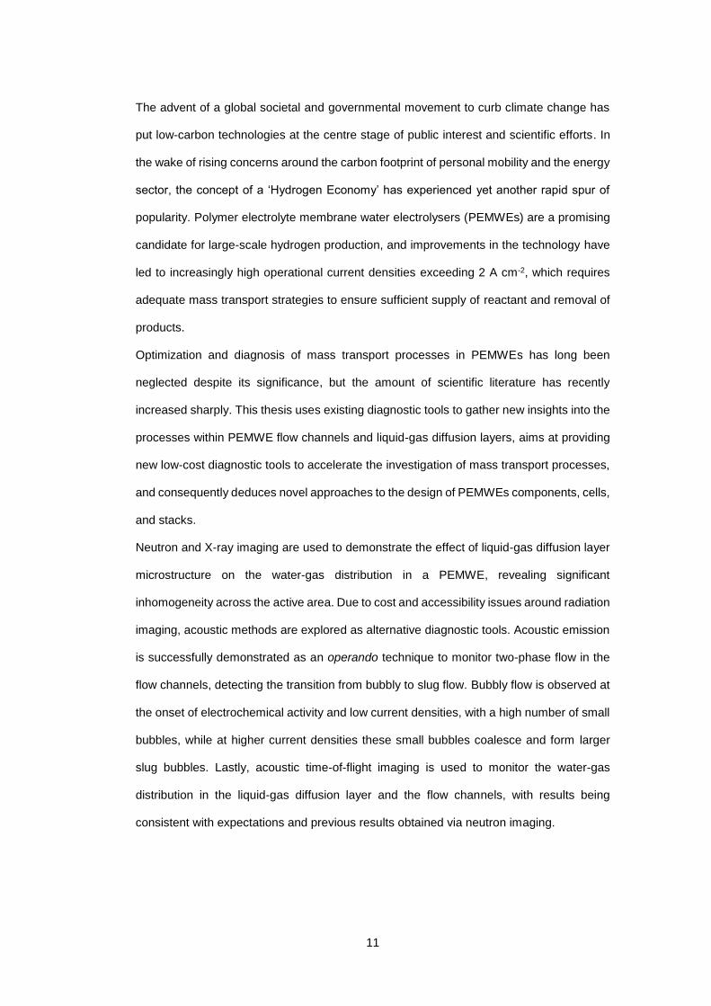
The advent of a global societal and governmental movement to curb climate change has
put low-carbon technologies at the centre stage of public interest and scientific efforts. In
the wake of rising concerns around the carbon footprint of personal mobility and the energy
sector, the concept of a ‘Hydrogen Economy’ has experienced yet another rapid spur of
popularity. Polymer electrolyte membrane water electrolysers (PEMWEs) are a promising
candidate for large-scale hydrogen production, and improvements in the technology have
led to increasingly high operational current densities exceeding 2 A cm-2, which requires
adequate mass transport strategies to ensure sufficient supply of reactant and removal of
products.
Optimization and diagnosis of mass transport processes in PEMWEs has long been
neglected despite its significance, but the amount of scientific literature has recently
increased sharply. This thesis uses existing diagnostic tools to gather new insights into the
processes within PEMWE flow channels and liquid-gas diffusion layers, aims at providing
new low-cost diagnostic tools to accelerate the investigation of mass transport processes,
and consequently deduces novel approaches to the design of PEMWEs components, cells,
and stacks.
Neutron and X-ray imaging are used to demonstrate the effect of liquid-gas diffusion layer
microstructure on the water-gas distribution in a PEMWE, revealing significant
inhomogeneity across the active area. Due to cost and accessibility issues around radiation
imaging, acoustic methods are explored as alternative diagnostic tools. Acoustic emission
is successfully demonstrated as an operando technique to monitor two-phase flow in the
flow channels, detecting the transition from bubbly to slug flow. Bubbly flow is observed at
the onset of electrochemical activity and low current densities, with a high number of small
bubbles, while at higher current densities these small bubbles coalesce and form larger
slug bubbles. Lastly, acoustic time-of-flight imaging is used to monitor the water-gas
distribution in the liquid-gas diffusion layer and the flow channels, with results being
consistent with expectations and previous results obtained via neutron imaging.


13
Impact Statement

15
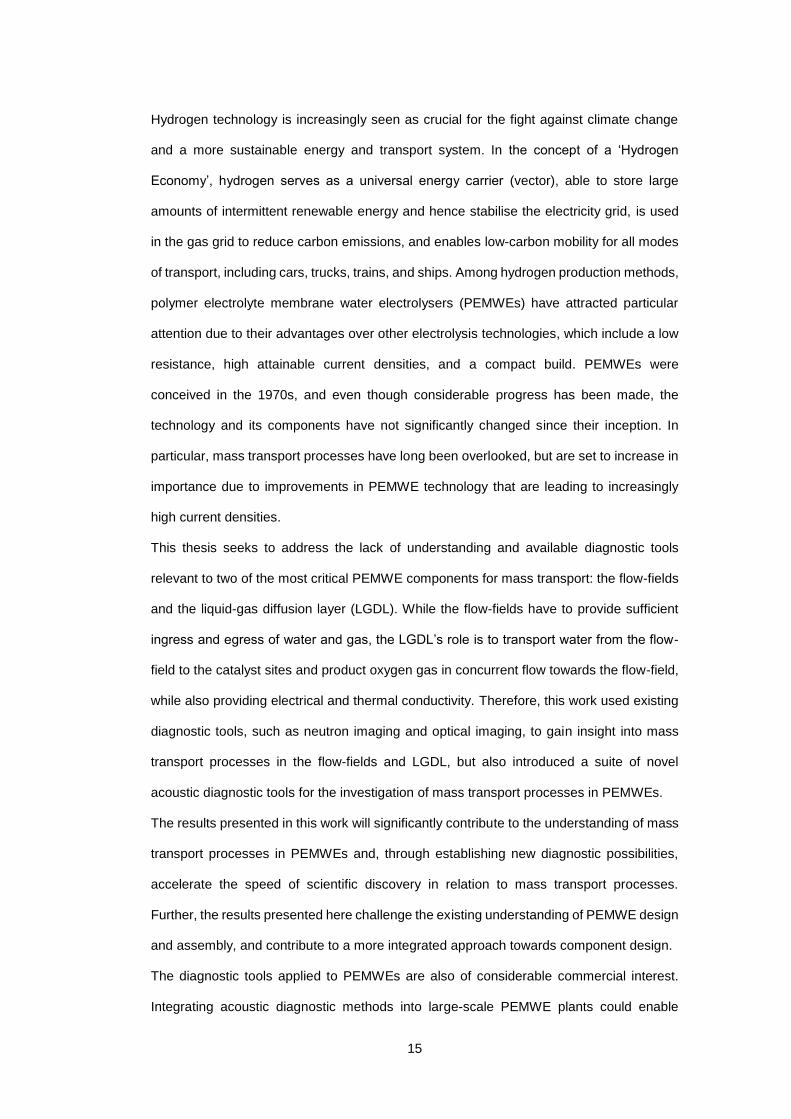
Hydrogen technology is increasingly seen as crucial for the fight against climate change
and a more sustainable energy and transport system. In the concept of a ‘Hydrogen
Economy’, hydrogen serves as a universal energy carrier (vector), able to store large
amounts of intermittent renewable energy and hence stabilise the electricity grid, is used
in the gas grid to reduce carbon emissions, and enables low-carbon mobility for all modes
of transport, including cars, trucks, trains, and ships. Among hydrogen production methods,
polymer electrolyte membrane water electrolysers (PEMWEs) have attracted particular
attention due to their advantages over other electrolysis technologies, which include a low
resistance, high attainable current densities, and a compact build. PEMWEs were
conceived in the 1970s, and even though considerable progress has been made, the
technology and its components have not significantly changed since their inception. In
particular, mass transport processes have long been overlooked, but are set to increase in
importance due to improvements in PEMWE technology that are leading to increasingly
high current densities.
This thesis seeks to address the lack of understanding and available diagnostic tools
relevant to two of the most critical PEMWE components for mass transport: the flow-fields
and the liquid-gas diffusion layer (LGDL). While the flow-fields have to provide sufficient
ingress and egress of water and gas, the LGDL’s role is to transport water from the flow-
field to the catalyst sites and product oxygen gas in concurrent flow towards the flow-field,
while also providing electrical and thermal conductivity. Therefore, this work used existing
diagnostic tools, such as neutron imaging and optical imaging, to gain insight into mass
transport processes in the flow-fields and LGDL, but also introduced a suite of novel
acoustic diagnostic tools for the investigation of mass transport processes in PEMWEs.
The results presented in this work will significantly contribute to the understanding of mass
transport processes in PEMWEs and, through establishing new diagnostic possibilities,
accelerate the speed of scientific discovery in relation to mass transport processes.
Further, the results presented here challenge the existing understanding of PEMWE design
and assembly, and contribute to a more integrated approach towards component design.
The diagnostic tools applied to PEMWEs are also of considerable commercial interest.
Integrating acoustic diagnostic methods into large-scale PEMWE plants could enable

16
optimized operation and real-time adjustment of local inefficiencies, such as bubble
blockage or insufficient water supply. Further, the two acoustic diagnostic tools investigated
in this work could successfully be employed for a range of applications in the chemical
industry, leveraging their demonstrated suitability to monitor multi-phase systems in real-
time, at low-cost, and in a non-destructive manner.
The results presented in this thesis have been disseminated in four first-author peer-
reviewed publications in internationally renowned journals, and conferences including the
235th ECS Meeting in Dallas (USA) and the 22nd World Hydrogen Economic Forum (WHEC)
in Rio de Janeiro (Brazil). Academic collaborators included researchers from the National
Physics Laboratory (UK), the Helmholtz Zentrum Berlin (Germany), and the School of
Chemistry at the University of New South Wales (Australia).

17
Table of Contents

19
Table of Contents Acknowledgements ................................................................................. 5
Abstract .................................................................................................... 9
Impact Statement ................................................................................... 13
Table of Contents ................................................................................... 17
List of Tables .......................................................................................... 23
List of Figures ........................................................................................ 27
List of Abbreviations and Nomenclature ............................................. 39
1 Introduction ..................................................................................... 45
1.1 Background ....................................................................................................... 47
1.2 PEM Water Electrolysers .................................................................................. 51
1.3 Mass Transport Limitations in PEMWEs ........................................................... 54
1.4 Research Motivation ......................................................................................... 55
1.5 Thesis Overview ................................................................................................ 57
2 Fundamentals of PEMWE Operation ............................................. 59
2.1 Overview ........................................................................................................... 61
2.2 PEMWE Cell Assembly ..................................................................................... 62
2.3 Sources of Voltage Loss in a PEMWE .............................................................. 65
2.4 PEMWE Catalysts and Membrane ................................................................... 68
2.4.1 Electrocatalysts ......................................................................................... 68
2.4.2 Membrane and Ionomer ............................................................................ 68
3 Literature Review ............................................................................ 71
3.1 Overview ........................................................................................................... 73
3.2 Mass Transport in the Flow Channels .............................................................. 74
3.2.1 Flow Regime ............................................................................................. 74
3.2.2 Mass Flux .................................................................................................. 75
3.2.3 Flow-Field Design and Diagnostics ........................................................... 79
3.2.4 Influence of the Flow Regime on Performance ......................................... 81
3.2.5 Two-Phase Modelling ................................................................................ 83
3.3 Mass Transport in the Liquid-Gas Diffusion Layer ............................................ 85
3.3.1 Liquid-Gas Diffusion Layer Materials ........................................................ 85
3.3.2 Micro-Porous Layers and Surface Modifications ...................................... 89
3.3.2.1 Micro-Porous Layers ............................................................................. 90
3.3.2.2 Surface and Structural Modifications .................................................... 91
20
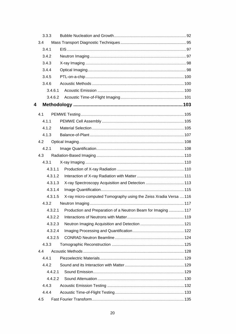
3.3.3 Bubble Nucleation and Growth .................................................................. 92
3.4 Mass Transport Diagnostic Techniques ............................................................ 95
3.4.1 EIS ............................................................................................................. 97
3.4.2 Neutron Imaging ........................................................................................ 97
3.4.3 X-ray Imaging ............................................................................................ 98
3.4.4 Optical Imaging .......................................................................................... 98
3.4.5 PTL-on-a-chip .......................................................................................... 100
3.4.6 Acoustic Methods .................................................................................... 100
3.4.6.1 Acoustic Emission ............................................................................... 100
3.4.6.2 Acoustic Time-of-Flight Imaging .......................................................... 101
4 Methodology .................................................................................. 103
4.1 PEMWE Testing .............................................................................................. 105
4.1.1 PEMWE Cell Assembly ........................................................................... 105
4.1.2 Material Selection .................................................................................... 105
4.1.3 Balance-of-Plant ...................................................................................... 107
4.2 Optical Imaging ................................................................................................ 108
4.2.1 Image Quantification ................................................................................ 108
4.3 Radiation-Based Imaging ................................................................................ 110
4.3.1 X-ray Imaging .......................................................................................... 110
4.3.1.1 Production of X-ray Radiation ............................................................. 110
4.3.1.2 Interaction of X-ray Radiation with Matter ........................................... 111
4.3.1.3 X-ray Spectroscopy Acquisition and Detection ................................... 113
4.3.1.4 Image Quantification ............................................................................ 115
4.3.1.5 X-ray micro-computed Tomography using the Zeiss Xradia Versa .... 116
4.3.2 Neutron Imaging ...................................................................................... 117
4.3.2.1 Production and Preparation of a Neutron Beam for Imaging .............. 117
4.3.2.2 Interactions of Neutrons with Matter .................................................... 119
4.3.2.3 Neutron Imaging Acquisition and Detection ........................................ 121
4.3.2.4 Imaging Processing and Quantification ............................................... 122
4.3.2.5 CONRAD Neutron Beamline ............................................................... 124
4.3.3 Tomographic Reconstruction .................................................................. 125
4.4 Acoustic Methods ............................................................................................ 128
4.4.1 Piezoelectric Materials............................................................................. 129
4.4.2 Sound and its Interaction with Matter ...................................................... 129
4.4.2.1 Sound Emission ................................................................................... 129
4.4.2.2 Sound Attenuation ............................................................................... 130
4.4.3 Acoustic Emission Testing ...................................................................... 132
4.4.4 Acoustic Time-of-Flight Testing ............................................................... 133
4.5 Fast Fourier Transform .................................................................................... 135
21
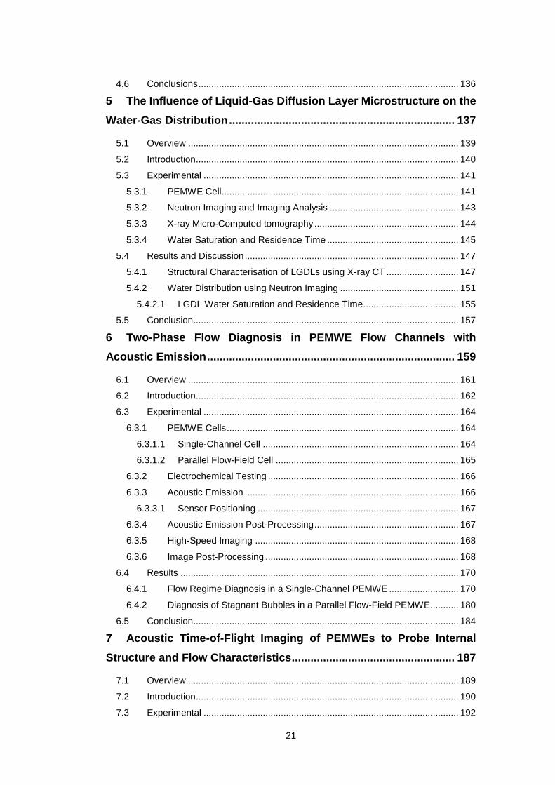
4.6 Conclusions ..................................................................................................... 136
5 The Influence of Liquid-Gas Diffusion Layer Microstructure on the
Water-Gas Distribution ........................................................................ 137
5.1 Overview ......................................................................................................... 139
5.2 Introduction ...................................................................................................... 140
5.3 Experimental ................................................................................................... 141
5.3.1 PEMWE Cell ............................................................................................ 141
5.3.2 Neutron Imaging and Imaging Analysis .................................................. 143
5.3.3 X-ray Micro-Computed tomography ........................................................ 144
5.3.4 Water Saturation and Residence Time ................................................... 145
5.4 Results and Discussion ................................................................................... 147
5.4.1 Structural Characterisation of LGDLs using X-ray CT ............................ 147
5.4.2 Water Distribution using Neutron Imaging .............................................. 151
5.4.2.1 LGDL Water Saturation and Residence Time ..................................... 155
5.5 Conclusion ....................................................................................................... 157
6 Two-Phase Flow Diagnosis in PEMWE Flow Channels with
Acoustic Emission ............................................................................... 159
6.1 Overview ......................................................................................................... 161
6.2 Introduction ...................................................................................................... 162
6.3 Experimental ................................................................................................... 164
6.3.1 PEMWE Cells .......................................................................................... 164
6.3.1.1 Single-Channel Cell ............................................................................ 164
6.3.1.2 Parallel Flow-Field Cell ....................................................................... 165
6.3.2 Electrochemical Testing .......................................................................... 166
6.3.3 Acoustic Emission ................................................................................... 166
6.3.3.1 Sensor Positioning .............................................................................. 167
6.3.4 Acoustic Emission Post-Processing ........................................................ 167
6.3.5 High-Speed Imaging ............................................................................... 168
6.3.6 Image Post-Processing ........................................................................... 168
6.4 Results ............................................................................................................ 170
6.4.1 Flow Regime Diagnosis in a Single-Channel PEMWE ........................... 170
6.4.2 Diagnosis of Stagnant Bubbles in a Parallel Flow-Field PEMWE ........... 180
6.5 Conclusion ....................................................................................................... 184
7 Acoustic Time-of-Flight Imaging of PEMWEs to Probe Internal
Structure and Flow Characteristics .................................................... 187
7.1 Overview ......................................................................................................... 189
7.2 Introduction ...................................................................................................... 190
7.3 Experimental ................................................................................................... 192
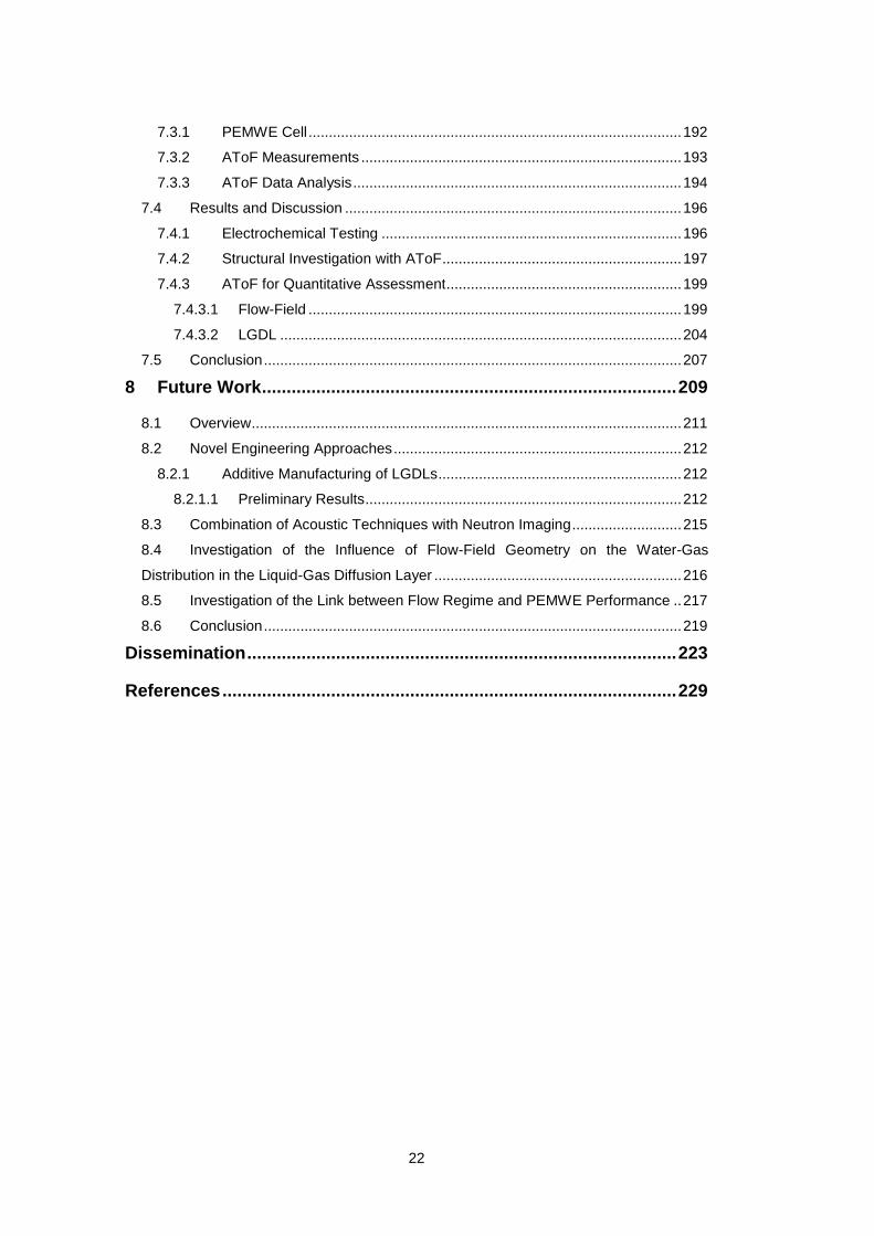
22
7.3.1 PEMWE Cell ............................................................................................ 192
7.3.2 AToF Measurements ............................................................................... 193
7.3.3 AToF Data Analysis ................................................................................. 194
7.4 Results and Discussion ................................................................................... 196
7.4.1 Electrochemical Testing .......................................................................... 196
7.4.2 Structural Investigation with AToF ........................................................... 197
7.4.3 AToF for Quantitative Assessment .......................................................... 199
7.4.3.1 Flow-Field ............................................................................................ 199
7.4.3.2 LGDL ................................................................................................... 204
7.5 Conclusion ....................................................................................................... 207
8 Future Work .................................................................................... 209
8.1 Overview .......................................................................................................... 211
8.2 Novel Engineering Approaches ....................................................................... 212
8.2.1 Additive Manufacturing of LGDLs ............................................................ 212
8.2.1.1 Preliminary Results .............................................................................. 212
8.3 Combination of Acoustic Techniques with Neutron Imaging ........................... 215
8.4 Investigation of the Influence of Flow-Field Geometry on the Water-Gas
Distribution in the Liquid-Gas Diffusion Layer ............................................................. 216
8.5 Investigation of the Link between Flow Regime and PEMWE Performance .. 217
8.6 Conclusion ....................................................................................................... 219
Dissemination ....................................................................................... 223
References ............................................................................................ 229

23
List of Tables

25
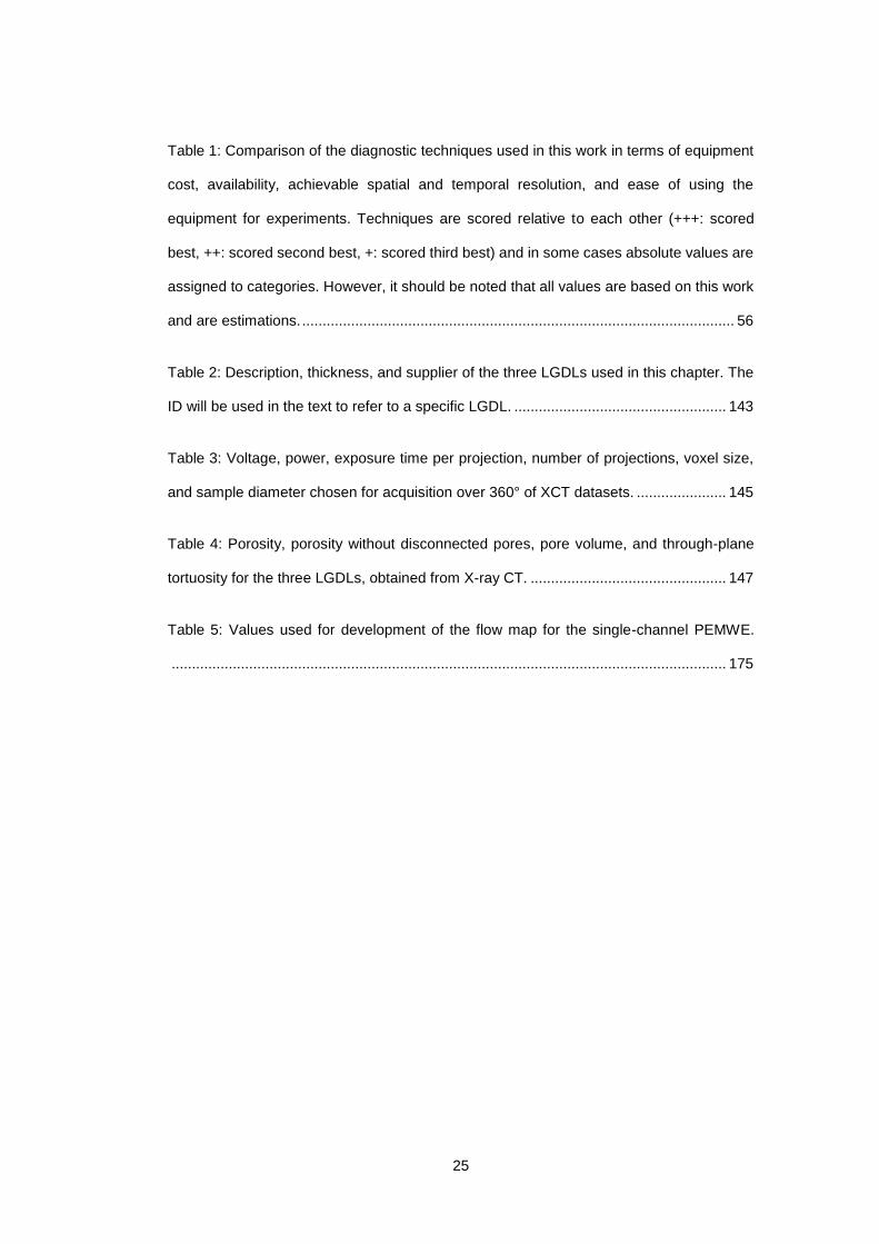
Table 1: Comparison of the diagnostic techniques used in this work in terms of equipment
cost, availability, achievable spatial and temporal resolution, and ease of using the
equipment for experiments. Techniques are scored relative to each other (+++: scored
best, ++: scored second best, +: scored third best) and in some cases absolute values are
assigned to categories. However, it should be noted that all values are based on this work
and are estimations. .......................................................................................................... 56
Table 2: Description, thickness, and supplier of the three LGDLs used in this chapter. The
ID will be used in the text to refer to a specific LGDL. .................................................... 143
Table 3: Voltage, power, exposure time per projection, number of projections, voxel size,
and sample diameter chosen for acquisition over 360° of XCT datasets. ...................... 145
Table 4: Porosity, porosity without disconnected pores, pore volume, and through-plane
tortuosity for the three LGDLs, obtained from X-ray CT. ................................................ 147
Table 5: Values used for development of the flow map for the single-channel PEMWE.
........................................................................................................................................ 175


27
List of Figures

29
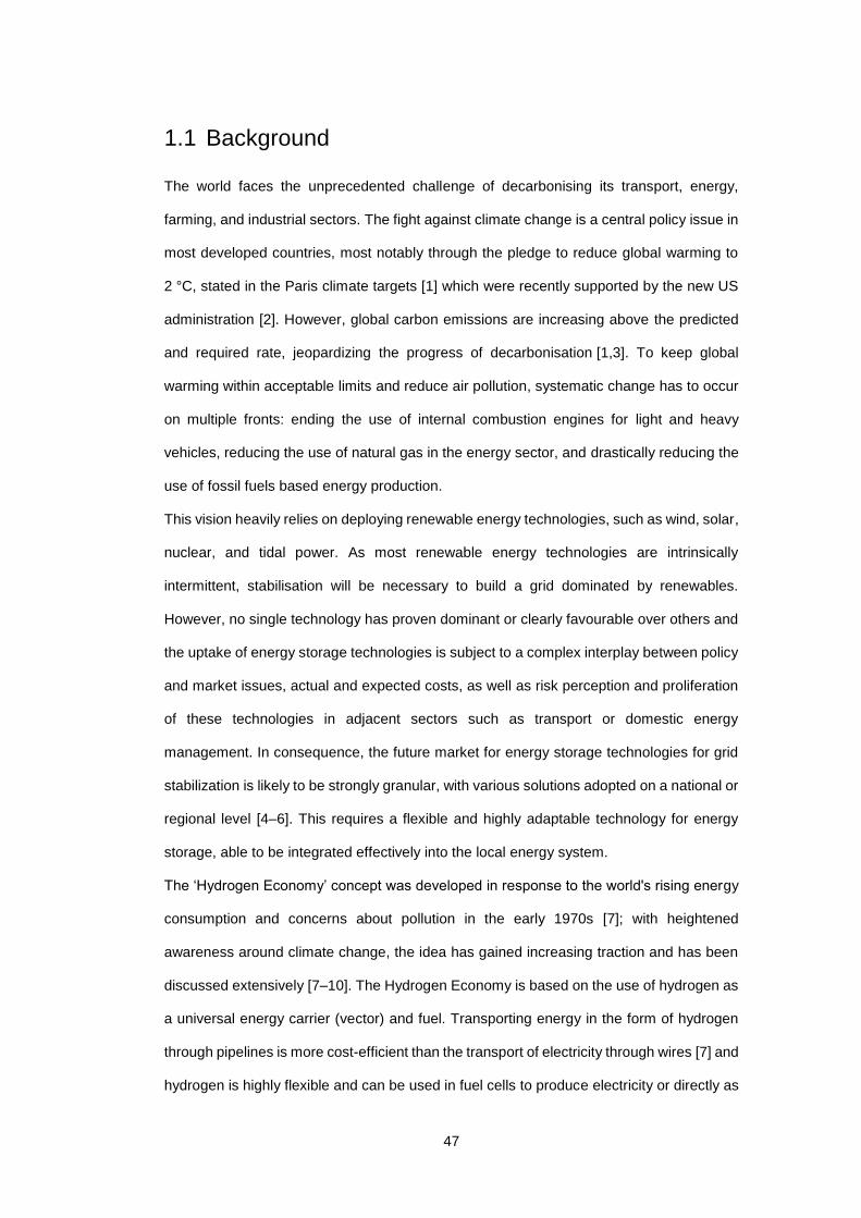
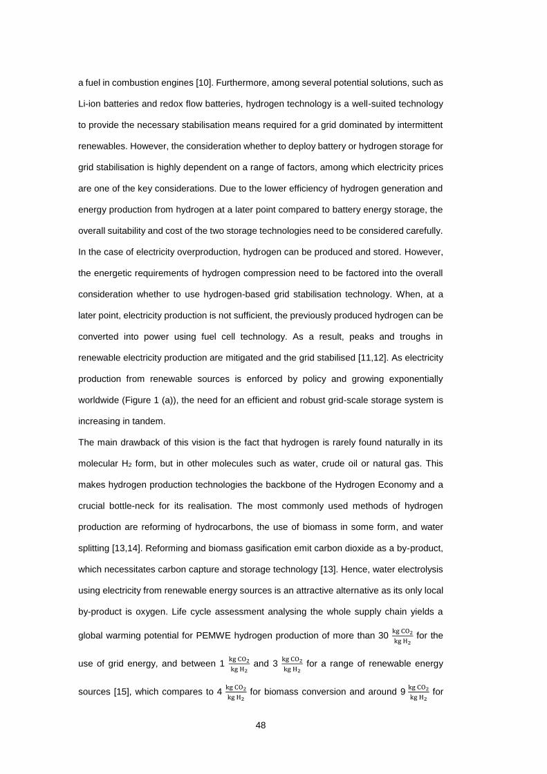
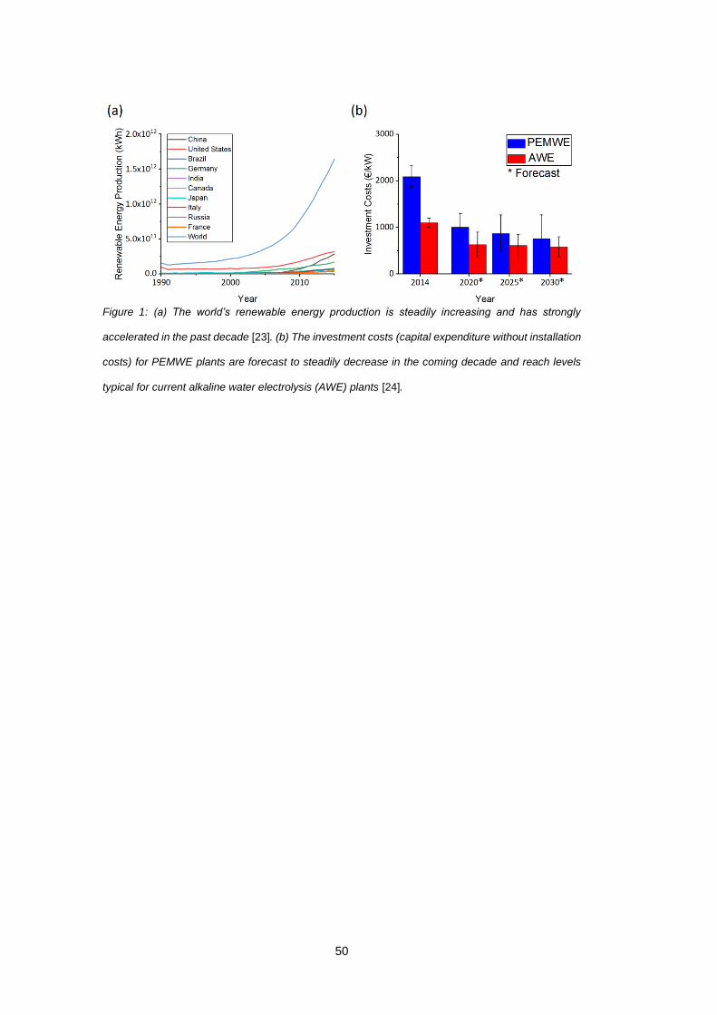
Figure 1: (a) The world’s renewable energy production is steadily increasing and has
strongly accelerated in the past decade [23]. (b) The investment costs (capital expenditure
without installation costs) for PEMWE plants are forecast to steadily decrease in the coming
decade and reach levels typical for current alkaline water electrolysis (AWE) plants [24].
.......................................................................................................................................... 50
Figure 2: (a) PEMWEs rely on a solid polymer membrane through which protons are
transported from the anode to the cathode, while for (b) alkaline water electrolysers (AWEs)
a liquid electrolyte is used and hydroxyl ions move from cathode to anode (adapted from
[18]). .................................................................................................................................. 51
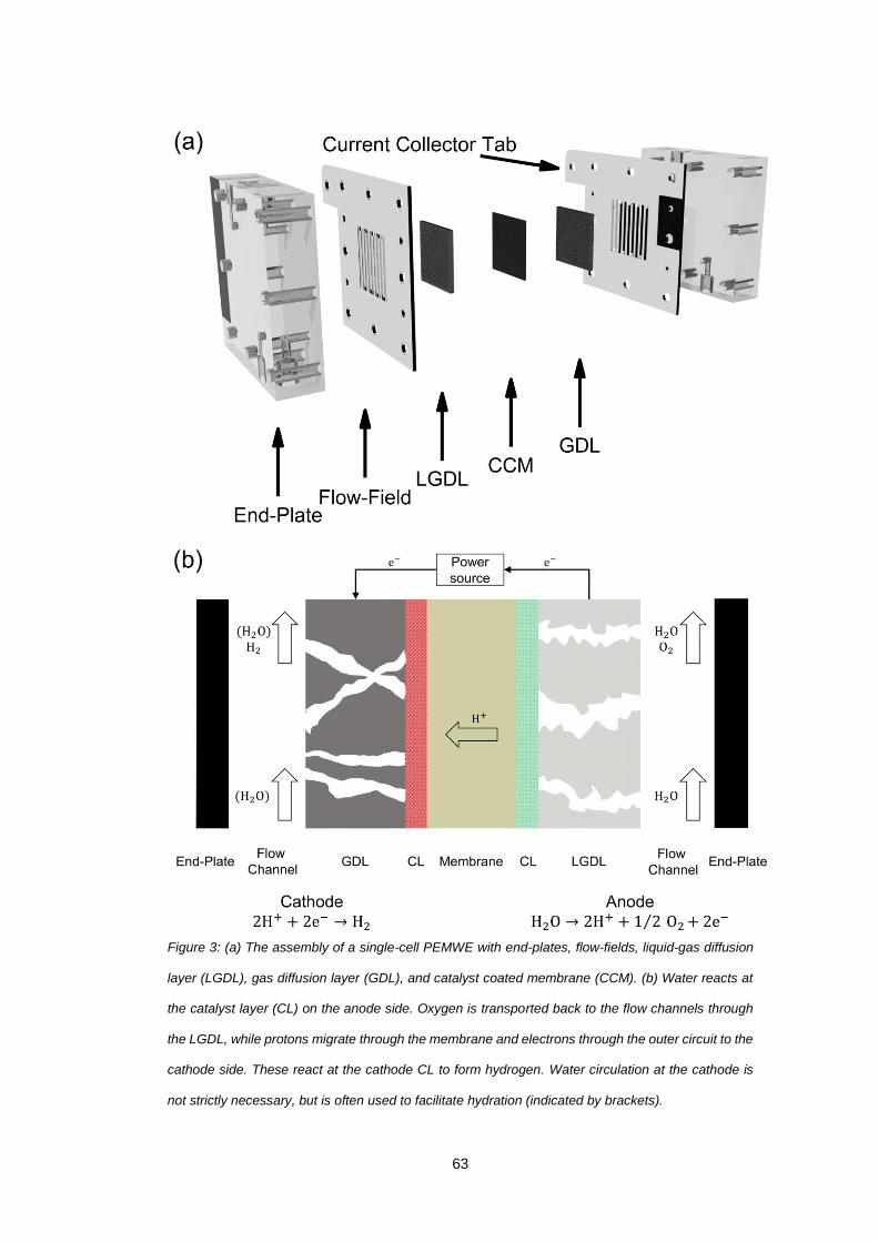
Figure 3: (a) The assembly of a single-cell PEMWE with end-plates, flow-fields, liquid-gas
diffusion layer (LGDL), gas diffusion layer (GDL), and catalyst coated membrane (CCM).
(b) Water reacts at the catalyst layer (CL) on the anode side. Oxygen is transported back
to the flow channels through the LGDL, while protons migrate through the membrane and
electrons through the outer circuit to the cathode side. These react at the cathode CL to
form hydrogen. Water circulation at the cathode is not strictly necessary, but is often used
to facilitate hydration (indicated by brackets). ................................................................... 63
Figure 4: (a) Polarisation curve of a PEMWE at different temperatures [62] (Reprinted from
‘J Power Sources, 396, Yang et al., Bipolar plate development with additive manufacturing
and protective coating for durable and high-efficiency hydrogen production, 590–8, 2018’,
with permission from Elsevier). (b) Theoretical polarisation curve, predicting rapid voltage
increase due to the concentration overvoltage [52] (Reprinted from ‘Int J Hydrogen Energy,
42, Han et al., Modeling of two-phase transport in proton exchange membrane electrolyzer
cells for hydrogen energy, 4478–89, 2017’, with permission from Elsevier). ................... 67
Figure 5: Chemical structure of Nafion, consisting of a tetrafluoroethylene backbone and
side chains carrying a sulfonic acid group [64]. (Reprinted with permission from Mauritz
KA, Moore RB. Chem Rev. 104:4535–85. Copyright (2004) American Chemical Society.)
.......................................................................................................................................... 69
30
Figure 6: With increasing current density, more gas is produced and has to be removed
through the flow channels. The flow regime progresses from bubble to plug, slug, churn
and annular regime. .......................................................................................................... 75
Figure 7: (a) Comparison of the mass fluxes of water with the oxygen generation in the
range from 0 A cm-2 to 3 A cm-2 at a water circulation rate of 50 ml min-1 and a temperature
of 90 °C, in a parallel flow-field with 9 channels (Width: 1.76 mm, Depth: 2.00 mm). The
gravimetric gas fraction at the outlet increases linearly with current density. (b) Water ratio
as a function of current density at the same conditions, for water circulation rates of 5 ml
min-1, 50 ml min-1, and 100 ml min-1. ................................................................................. 77
Figure 8: The flow maps of (a) Cubaud et al. [67] (Reprinted from ‘Cubaud et al., Transport
of bubbles in square microchannels. Phys Fluids 2004;16:4575–85.’, with the permission
of AIP Publishing.) and (b) Mishima et al. [65] (Reprinted from ‘Int J Multiph Flow, 22,
Mishima et al., Some characteristics of air-water two-phase flow in small diameter vertical
tubes, 703–12’, with permission from Elsevier), defining the occurrence of various flow
regimes as a function of the velocity of the liquid and gas phase in the flow channels. The
shape and location of the regime borders vary depending on the exact shape and size of
the channels of the experimental systems used to create the flow map........................... 78
Figure 9: Perspective (a-c) and top-down (d-f) view of a parallel (a,d,g), single-serpentine
(b,e,h), and triple-serpentine (c,f,i) flow-field. The gas and liquid amount in each channel
along its length (g-i) varies depending on the flow-field geometry. The channel number is
indicated in (d-f) and used accordingly in (g-i). The axis titles on the left and right of (g-i)
apply to all three figures. ................................................................................................... 79
Figure 10: SEM images and X-ray tomograms of various materials that can be used as an
LGDL in PEMWEs. (a) Sintered powder and (b) fibrous materials are commonly employed,
while (c) perforated plates are very useful for optical access to the catalyst surface, and (d)
metal foams have shown promise in unitized reversible fuel cells. ................................... 87
Figure 11: Examples of commonly used diagnostic techniques: (a) Nyquist diagram
31
produced from electrochemical impedance spectroscopy and an equivalent circuit, (b)
through-plane water thickness measurement via neutron radiography, (c) X-ray computed
tomography of a sintered and a fibrous LGDL material, (d) X-ray synchrotron radiography
of channel and land areas in a PEMWE [84] (Reprinted from ‘Electrochimica Acta, 276,
Leonard et al., Operando X-ray tomography and sub-second radiography for characterizing
transport in polymer electrolyte membrane electrolyzer, 424–33, 2018’ with permission
from Elsevier), (e) image obtained during a PTL-on-a-chip experiment [160] (Reprinted
from ‘J Power Sources, 258, Arbabi et al., Feasibility study of using microfluidic platforms
for visualizing bubble flows in electrolyzer gas diffusion layers, 142–9, 2014’ with
permission from Elsevier), and (f) high-speed optical imaging of bubble nucleation along
the triple-phase boundary of catalyst, LGDL, and water [80] (Reprinted with permission
under a CC BY-NC licence (https://creativecommons.org/licenses/by-nc/4.0/legalcode)
from ‘Mo et al., Sci Adv 2016;2:e1600690–e1600690,
https://advances.sciencemag.org/content/2/11/e1600690’. Copyright (2016) American
Association for the Advancement of Science). ................................................................. 96
Figure 12: Pourbaix diagrams of (a) titanium (Republished with permission of NACE
International – Corrosion Society, from [217] ‘Atlas of electrochemical equilibria in aqueous
solutions. Pourbaix M., 1974’, permission conveyed through Copyright Clearance Center,
Inc.) and (b) iron in iron-chromium-nickel at 25 °C (Republished with permission of National
Association of Corrosion Engineers, from [216] ‘Pourbaix diagrams for the ternary system
of iron-chromium-nickel, Beverskog et al., Corrosion, 55, 1077–87, 1999’; permission
conveyed through Copyright Clearance Center, Inc,), illustrating the corrosion behaviour of
both metals as a function of pH and potential. ................................................................ 106
Figure 13: Process diagram of the balance-of-plant used for PEMWE testing. Solid lines
denote liquid flows, while dashed lines indicate gas flows. The potentiostat is connected to
anode and cathode simultaneously. ............................................................................... 107
Figure 14: Illustration of the use of the algorithm for analysis of bubbly (a-d) and slug (e-h)
flow for detection of bubble sizes and numbers. Raw images (a, e) are thresholded and
32
filtered (b, f), circular structures are identified (c, g) and finally, overlapping circles are
removed (d, h). Good bubble identification can be observed for bubbly flow, while the
algorithms limitations are visible in slug flow. Only the minor axis of elliptical bubbles is
measured and the overall detection accuracy was reduced. .......................................... 109
Figure 15: Overview of the interaction of an X-ray beam with a sample. The incident X-ray
beam is attenuated due to a number of mechanisms, of which the photoelectric effect is
dominant in the energy range relevant to X-ray spectroscopy. The transmitted portion of
the X-ray beam is then detected [227]. ........................................................................... 112
Figure 16: During acquisition of an X-ray tomography, the sample is rotated in an X-ray
beam and the sample projection is captured on a scintillator screen. Here, acquisition with
a cone beam is displayed, however, a parallel beam (typically at a synchrotron) can be
used as well (adapted from [230]). .................................................................................. 114
Figure 17: (a) The Zeiss Xradia Versa XRM-520T [236]. (b) Inside the Versa chamber a
sample (2) is rotated during tomographic acquisition. The projections are captured with a
detection system (4), with the optical magnification being adaptable by selecting one lens
from the magnification turret (3). To mitigate beam hardening effects, a range of X-ray filters
can be used (1) (adapted from [236]). ............................................................................ 117
Figure 18: Neutron flux as a function of wavelength (in Å) for hot, thermal, and cold
neutrons. (Reprinted from [237], with the permission of AIP Publishing.)....................... 119
Figure 19: Attenuation coefficients as a function of the atomic number for thermal neutrons
and X-rays. While the attenuation coefficient towards X-ray radiation is a continuous
function of the atomic number, the neutron attenuation coefficient is non-continuous [241]
(Reprinted from Journal of Neutron Research. Vol 14. Kardjilov et al. Neutron tomography
for archaeological investigations. 29–36. 2006, with permission from IOS Press. The
publication is available at IOS Press through http://dx.doi.org/
10.1080/10238160600673201). ...................................................................................... 121
Figure 20: (a) The PEMWE is placed in a neutron beam. Due to the material-dependent
33
attenuation of the neutrons, a radiographic image of the PEMWE is captured by the
detector. (b) Each set of images is first filtered to remove outliers and averaged using a
median. Then, the averaged dark-field is subtracted from the resulting image. This is then
normalized with a dry image (also averaged) to obtain the final image. The greyscale values
can be converted into the water thickness using the Beer-Lambert law. (c) The water
thickness in the rib (land) areas is analysed separately by applying a mask, discarding the
water thickness in the flow channels. .............................................................................. 123
Figure 21: (a) The hutch setup at the CONRAD beamline HZB with collimated neutron
beam, sample, and detector (Reprinted with permission under a CC BY 4.0 licence
(https://creativecommons.org/licenses/by/4.0/legalcode) from [243] ‘Kardjilov N et al., J
Large-Scale Res Facil JLSRF, 2:2–7, https://jlsrf.org/index.php/lsf/article/view/108’.
Copyright (2016) Journal of Large-Scale Research Facilities). (b) The neutron beam
spectrum at CONRAD with a peak around 3 Å (Reproduced from [244] with permission of
the International Union of Crystallography)..................................................................... 125
Figure 22: Visualisation of the tomographic reconstruction problem. The projection 𝑝, which
is measured by the detector, is the summation of the attenuation coefficients 𝜇 of the
elements on the beam path [232]. .................................................................................. 126
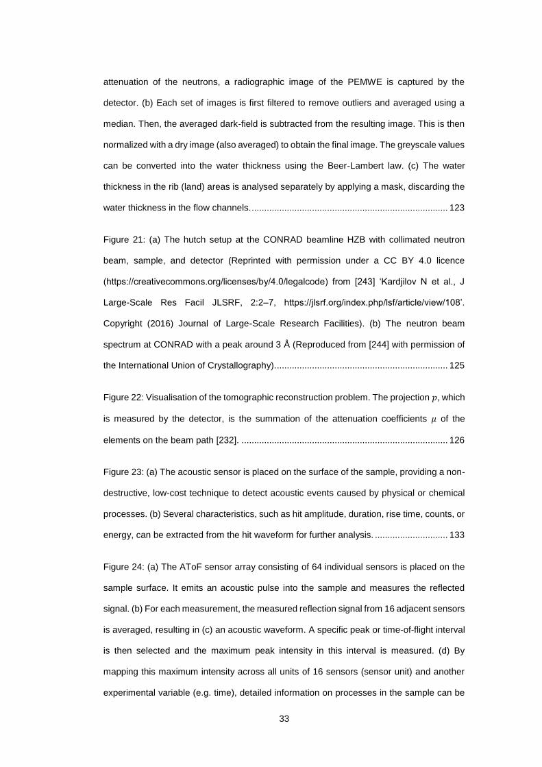
Figure 23: (a) The acoustic sensor is placed on the surface of the sample, providing a non-
destructive, low-cost technique to detect acoustic events caused by physical or chemical
processes. (b) Several characteristics, such as hit amplitude, duration, rise time, counts, or
energy, can be extracted from the hit waveform for further analysis. ............................. 133
Figure 24: (a) The AToF sensor array consisting of 64 individual sensors is placed on the
sample surface. It emits an acoustic pulse into the sample and measures the reflected
signal. (b) For each measurement, the measured reflection signal from 16 adjacent sensors
is averaged, resulting in (c) an acoustic waveform. A specific peak or time-of-flight interval
is then selected and the maximum peak intensity in this interval is measured. (d) By
mapping this maximum intensity across all units of 16 sensors (sensor unit) and another
experimental variable (e.g. time), detailed information on processes in the sample can be
34
obtained. .......................................................................................................................... 134
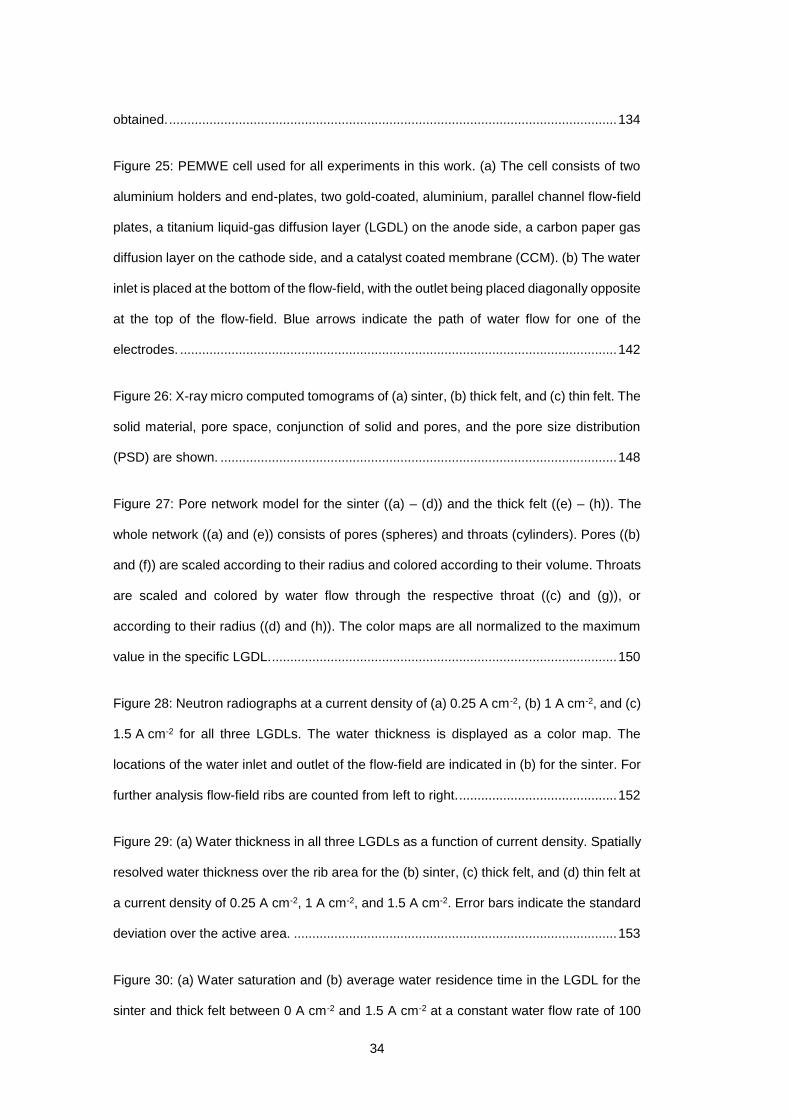
Figure 25: PEMWE cell used for all experiments in this work. (a) The cell consists of two
aluminium holders and end-plates, two gold-coated, aluminium, parallel channel flow-field
plates, a titanium liquid-gas diffusion layer (LGDL) on the anode side, a carbon paper gas
diffusion layer on the cathode side, and a catalyst coated membrane (CCM). (b) The water
inlet is placed at the bottom of the flow-field, with the outlet being placed diagonally opposite
at the top of the flow-field. Blue arrows indicate the path of water flow for one of the
electrodes. ....................................................................................................................... 142
Figure 26: X-ray micro computed tomograms of (a) sinter, (b) thick felt, and (c) thin felt. The
solid material, pore space, conjunction of solid and pores, and the pore size distribution
(PSD) are shown. ............................................................................................................ 148
Figure 27: Pore network model for the sinter ((a) – (d)) and the thick felt ((e) – (h)). The
whole network ((a) and (e)) consists of pores (spheres) and throats (cylinders). Pores ((b)
and (f)) are scaled according to their radius and colored according to their volume. Throats
are scaled and colored by water flow through the respective throat ((c) and (g)), or
according to their radius ((d) and (h)). The color maps are all normalized to the maximum
value in the specific LGDL. .............................................................................................. 150
Figure 28: Neutron radiographs at a current density of (a) 0.25 A cm-2, (b) 1 A cm-2, and (c)
1.5 A cm-2 for all three LGDLs. The water thickness is displayed as a color map. The
locations of the water inlet and outlet of the flow-field are indicated in (b) for the sinter. For
further analysis flow-field ribs are counted from left to right. ........................................... 152
Figure 29: (a) Water thickness in all three LGDLs as a function of current density. Spatially
resolved water thickness over the rib area for the (b) sinter, (c) thick felt, and (d) thin felt at
a current density of 0.25 A cm-2, 1 A cm-2, and 1.5 A cm-2. Error bars indicate the standard
deviation over the active area. ........................................................................................ 153
Figure 30: (a) Water saturation and (b) average water residence time in the LGDL for the
sinter and thick felt between 0 A cm-2 and 1.5 A cm-2 at a constant water flow rate of 100
35
ml min-1. Error bars indicate the standard deviation over the active area....................... 155
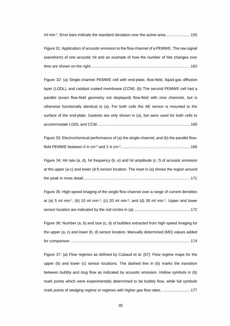
Figure 31: Application of acoustic emission to the flow channel of a PEMWE. The raw signal
(waveform) of one acoustic hit and an example of how the number of hits changes over
time are shown on the right. ............................................................................................ 163
Figure 32: (a) Single-channel PEMWE cell with end-plate, flow-field, liquid-gas diffusion
layer (LGDL), and catalyst coated membrane (CCM). (b) The second PEMWE cell had a
parallel (exact flow-field geometry not displayed) flow-field with nine channels, but is
otherwise functionally identical to (a). For both cells the AE sensor is mounted to the
surface of the end-plate. Gaskets are only shown in (a), but were used for both cells to
accommodate LGDL and CCM. ...................................................................................... 165
Figure 33: Electrochemical performance of (a) the single-channel, and (b) the parallel flow-
field PEMWE between 0 A cm-2 and 2 A cm-2. ................................................................ 166
Figure 34: Hit rate (a, d), hit frequency (b, e) and hit amplitude (c, f) of acoustic emission
at the upper (a-c) and lower (d-f) sensor location. The inset in (a) shows the region around
the peak in more detail. ................................................................................................... 171
Figure 35: High-speed imaging of the single flow channel over a range of current densities
at (a) 5 ml min-1, (b) 10 ml min-1, (c) 20 ml min-1, and (d) 30 ml min-1. Upper and lower
sensor location are indicated by the red circles in (a). .................................................... 172
Figure 36: Number (a, b) and size (c, d) of bubbles extracted from high-speed imaging for
the upper (a, c) and lower (b, d) sensor location. Manually determined (MD) values added
for comparison. ............................................................................................................... 174
Figure 37: (a) Flow regimes as defined by Cubaud et al. [67]. Flow regime maps for the
upper (b) and lower (c) sensor locations. The dashed line in (b) marks the transition
between bubbly and slug flow as indicated by acoustic emission. Hollow symbols in (b)
mark points which were experimentally determined to be bubbly flow, while full symbols
mark points of wedging regime or regimes with higher gas flow rates. .......................... 177
36
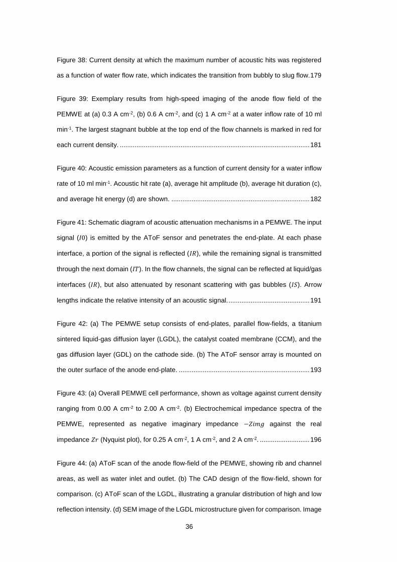
Figure 38: Current density at which the maximum number of acoustic hits was registered
as a function of water flow rate, which indicates the transition from bubbly to slug flow. 179
Figure 39: Exemplary results from high-speed imaging of the anode flow field of the
PEMWE at (a) 0.3 A cm-2, (b) 0.6 A cm-2, and (c) 1 A cm-2 at a water inflow rate of 10 ml
min-1. The largest stagnant bubble at the top end of the flow channels is marked in red for
each current density. ....................................................................................................... 181
Figure 40: Acoustic emission parameters as a function of current density for a water inflow
rate of 10 ml min-1. Acoustic hit rate (a), average hit amplitude (b), average hit duration (c),
and average hit energy (d) are shown. ........................................................................... 182
Figure 41: Schematic diagram of acoustic attenuation mechanisms in a PEMWE. The input
signal (𝐼0) is emitted by the AToF sensor and penetrates the end-plate. At each phase
interface, a portion of the signal is reflected (𝐼𝑅), while the remaining signal is transmitted
through the next domain (𝐼𝑇). In the flow channels, the signal can be reflected at liquid/gas
interfaces (𝐼𝑅), but also attenuated by resonant scattering with gas bubbles (𝐼𝑆). Arrow
lengths indicate the relative intensity of an acoustic signal. ............................................ 191
Figure 42: (a) The PEMWE setup consists of end-plates, parallel flow-fields, a titanium
sintered liquid-gas diffusion layer (LGDL), the catalyst coated membrane (CCM), and the
gas diffusion layer (GDL) on the cathode side. (b) The AToF sensor array is mounted on
the outer surface of the anode end-plate. ....................................................................... 193
Figure 43: (a) Overall PEMWE cell performance, shown as voltage against current density
ranging from 0.00 A cm-2 to 2.00 A cm-2. (b) Electrochemical impedance spectra of the
PEMWE, represented as negative imaginary impedance −𝑍𝑖𝑚𝑔 against the real
impedance 𝑍𝑟 (Nyquist plot), for 0.25 A cm-2, 1 A cm-2, and 2 A cm-2. ........................... 196
Figure 44: (a) AToF scan of the anode flow-field of the PEMWE, showing rib and channel
areas, as well as water inlet and outlet. (b) The CAD design of the flow-field, shown for
comparison. (c) AToF scan of the LGDL, illustrating a granular distribution of high and low
reflection intensity. (d) SEM image of the LGDL microstructure given for comparison. Image
37
was obtained on a Zeiss EVO MA10 (Carl Zeiss, USA) at an electron accelerating voltage
of 15 kV and a magnification of 100x. Both AToF area scans were obtained during
operation of the PEMWE at a constant current density of 0.25 A cm-2. Hence, water was
circulated through the flow-field, and LGDL and flow channels contained water as well as
oxygen. ............................................................................................................................ 198
Figure 45: (a) AToF reflection map of the flow-field across all flow channels at the middle
sensor location for current densities ranging from 0 A cm-2 to 2 A cm-2. This illustrates the
evolution of the reflection intensity in a segment across the width of the flow-field, roughly
the same height as the AToF sensor, as a function of current density. The intensity of the
reflection peaks is indicated using a logarithmic color map. Dashed black lines indicate
parabolic lines of identical intensity. (b) The average intensity of reflection peaks across all
flow channels for lower, middle, and upper sensor locations as a function of current density.
The average intensity band measured in the dry cell is shown for comparison (dashed black
lines). (c) For comparison, the inverse of the amount of oxygen per flow channel, G, is
shown as a function of current density for all three sensor locations. ............................ 201
Figure 46: The resonant scattering frequency of a bubble cloud with the diameter of a flow
channel for isothermal and adiabatic operation of the PEMWE as a function of current
density. The peak frequency of the AToF signal (obtained via FFT analysis) is shown as
single data points, which are consistent with the resonant scattering frequency. The lower
frequency detection limit is given for reference (dashed blue line). All calculations and
measurements refer to the middle sensor location. ........................................................ 204
Figure 47: (a) AToF reflection map across the LGDL width at the middle sensor location for
current densities ranging from 0 A cm-2 to 2 A cm-2. The intensity of the reflection peaks is
indicated using a linear color map. (b) Average intensity of reflection peaks across the
LGDL width for lower, middle, and upper sensor locations as a function of current density.
........................................................................................................................................ 205
Figure 48: (a) Performance, shown as i-V curves, between 0 A cm-2 and 2 A cm-2 of the
LGDLs with (b) cylindrical pores, (c) conical pores opening towards the CCM, and (d)
38
conical pores opening towards the flow channels. .......................................................... 213
Figure 49: P&ID of the balance-of-plant used for PEMWE testing with anode gas injection
to investigate the influence of the flow regime on electrochemical performance. Solid lines
denote liquid flows, while dashed lines indicate gas flows. The potentiostat is connected to
anode and cathode simultaneously. ................................................................................ 218

39
List of Abbreviations and Nomenclature

41
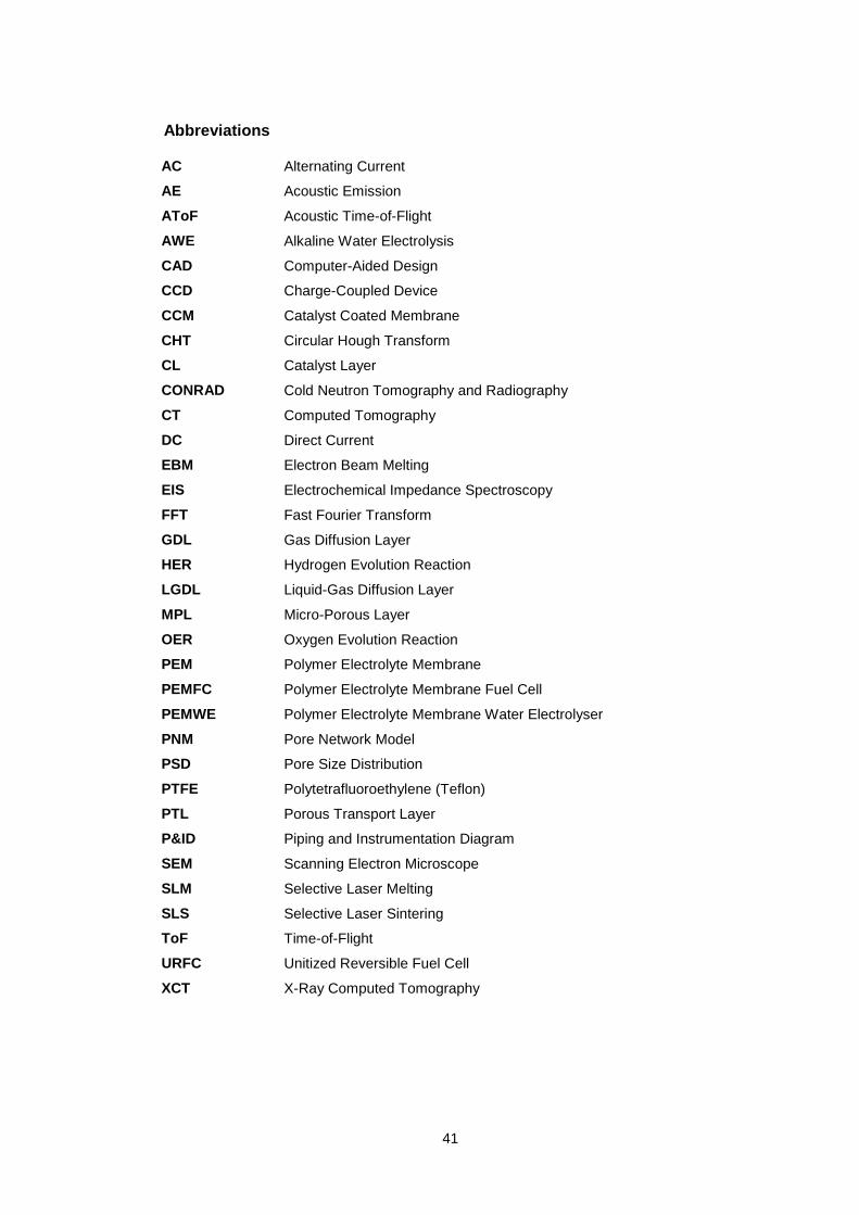
Abbreviations
AC Alternating Current
AE Acoustic Emission
AToF Acoustic Time-of-Flight
AWE Alkaline Water Electrolysis
CAD Computer-Aided Design
CCD Charge-Coupled Device
CCM Catalyst Coated Membrane
CHT Circular Hough Transform
CL Catalyst Layer
CONRAD Cold Neutron Tomography and Radiography
CT Computed Tomography
DC Direct Current
EBM Electron Beam Melting
EIS Electrochemical Impedance Spectroscopy
FFT Fast Fourier Transform
GDL Gas Diffusion Layer
HER Hydrogen Evolution Reaction
LGDL Liquid-Gas Diffusion Layer
MPL Micro-Porous Layer
OER Oxygen Evolution Reaction
PEM Polymer Electrolyte Membrane
PEMFC Polymer Electrolyte Membrane Fuel Cell
PEMWE Polymer Electrolyte Membrane Water Electrolyser
PNM Pore Network Model
PSD Pore Size Distribution
PTFE Polytetrafluoroethylene (Teflon)
PTL Porous Transport Layer
P&ID Piping and Instrumentation Diagram
SEM Scanning Electron Microscope
SLM Selective Laser Melting
SLS Selective Laser Sintering
ToF Time-of-Flight
URFC Unitized Reversible Fuel Cell
XCT X-Ray Computed Tomography

42
Nomenclature
𝑨 Peak Amplitude (-)
𝑨 Active Area (cm2)
𝑨(𝒏) Surface Area of a Cluster (m2)
𝒂 Thermodynamic Activity (-)
𝒂 Cross-Sectional Area of a Flow Channel (m2)
𝒂𝑽 Surface Area per Unit Volume (m2 m-3 or m-1)
𝒄 Concentration (mol m-3)
𝑫 Hit Duration (µs)
𝑫 Bubble Size (mm)
𝒅 LGDL Thickness (mm)
𝑬 Elastic Modulus (N mm-2 or Pa)
𝑬 External Electric Field (V m-1)
𝑬 Hit Energy (aJ)
𝒆 Induced Electric Field (V m-1)
𝑭 Faraday Constant (96485.3 C mol-1)
𝒇 Frequency (Hz or s-1)
𝑮 Gibb’s Free Energy (J)
𝑮 Mass Flux (kg s-1 m-2)
𝒈 Piezoelectric Voltage Constant (V m N-1)
𝑯 Hit Rate (s-1)
𝑰 Current (A)
𝑰 Intensity (-)
𝒊 Current Density (A cm-2)
𝒊𝟎 Exchange Current Density (A cm-2)
𝒋 Flow Velocity (m s-1)
𝑲 Permeability (m2)
𝒌 Wave Number (m-1)
𝒌𝑩 Boltzmann Constant (1.4 · 10-23 J K-1)
𝑴 Water Flow through LGDL (kg s-1)
𝑴 Molar Mass (kg mol-1)
𝑵 Number of Bubbles (-)
𝑵𝑨 Avogadro Constant (6.0 · 1023 mol-1)
𝒏𝑪 Critical Cluster Size (-)
𝒏𝒄𝒉𝒂𝒏 Number of Flow Channels (-)
𝒏𝒅𝒓𝒂𝒈 Electro-Osmotic Drag Coefficient (-)
𝒑 Pressure (Pa)
𝒑 Projection (m-1)
43
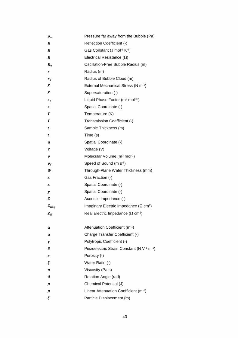
𝒑∞ Pressure far away from the Bubble (Pa)
𝑹 Reflection Coefficient (-)
𝑹 Gas Constant (J mol-1 K-1)
𝑹 Electrical Resistance (Ω)
𝑹𝟎 Oscillation-Free Bubble Radius (m)
𝒓 Radius (m)
𝒓𝑪 Radius of Bubble Cloud (m)
𝑺 External Mechanical Stress (N m-1)
𝑺 Supersaturation (-)
𝒔𝑳 Liquid Phase Factor (m2 mol2/3)
𝒔 Spatial Coordinate (-)
𝑻 Temperature (K)
𝑻 Transmission Coefficient (-)
𝒕 Sample Thickness (m)
𝒕 Time (s)
𝒖 Spatial Coordinate (-)
𝑽 Voltage (V)
𝒗 Molecular Volume (m3 mol-1)
𝒗𝑺 Speed of Sound (m s-1)
𝑾 Through-Plane Water Thickness (mm)
𝒙 Gas Fraction (-)
𝒙 Spatial Coordinate (-)
𝒚 Spatial Coordinate (-)
𝒁 Acoustic Impedance (-)
𝒁𝒊𝒎𝒈 Imaginary Electric Impedance (Ω cm2)
𝒁𝑹 Real Electric Impedance (Ω cm2)
𝜶 Attenuation Coefficient (m-1)
𝜶 Charge Transfer Coefficient (-)
𝜸 Polytropic Coefficient (-)
𝜹 Piezoelectric Strain Constant (N V-1 m-1)
𝜺 Porosity (-)
𝜻 Water Ratio (-)
𝜼 Viscosity (Pa s)
𝝑 Rotation Angle (rad)
𝝁 Chemical Potential (J)
𝝁 Linear Attenuation Coefficient (m-1)
𝝃 Particle Displacement (m)

44
𝝆 Density (kg m-3)
𝝈 Absorption Cross-Section (m2)
𝝈 Mechanical Strain (N m-2)
𝝈 Surface Tension (N m-1)
𝝉 Residence Time (s)
𝝉 Tortuosity (-)
𝝎 Angular Frequency (Hz or s-1)
𝕽 Radon Transform (-)

45
1 Introduction

47
1.1 Background
The world faces the unprecedented challenge of decarbonising its transport, energy,
farming, and industrial sectors. The fight against climate change is a central policy issue in
most developed countries, most notably through the pledge to reduce global warming to
2 °C, stated in the Paris climate targets [1] which were recently supported by the new US
administration [2]. However, global carbon emissions are increasing above the predicted
and required rate, jeopardizing the progress of decarbonisation [1,3]. To keep global
warming within acceptable limits and reduce air pollution, systematic change has to occur
on multiple fronts: ending the use of internal combustion engines for light and heavy
vehicles, reducing the use of natural gas in the energy sector, and drastically reducing the
use of fossil fuels based energy production.
This vision heavily relies on deploying renewable energy technologies, such as wind, solar,
nuclear, and tidal power. As most renewable energy technologies are intrinsically
intermittent, stabilisation will be necessary to build a grid dominated by renewables.
However, no single technology has proven dominant or clearly favourable over others and
the uptake of energy storage technologies is subject to a complex interplay between policy
and market issues, actual and expected costs, as well as risk perception and proliferation
of these technologies in adjacent sectors such as transport or domestic energy
management. In consequence, the future market for energy storage technologies for grid
stabilization is likely to be strongly granular, with various solutions adopted on a national or
regional level [4–6]. This requires a flexible and highly adaptable technology for energy
storage, able to be integrated effectively into the local energy system.
The ‘Hydrogen Economy’ concept was developed in response to the world's rising energy
consumption and concerns about pollution in the early 1970s [7]; with heightened
awareness around climate change, the idea has gained increasing traction and has been
discussed extensively [7–10]. The Hydrogen Economy is based on the use of hydrogen as
a universal energy carrier (vector) and fuel. Transporting energy in the form of hydrogen
through pipelines is more cost-efficient than the transport of electricity through wires [7] and
hydrogen is highly flexible and can be used in fuel cells to produce electricity or directly as
48
a fuel in combustion engines [10]. Furthermore, among several potential solutions, such as
Li-ion batteries and redox flow batteries, hydrogen technology is a well-suited technology
to provide the necessary stabilisation means required for a grid dominated by intermittent
renewables. However, the consideration whether to deploy battery or hydrogen storage for
grid stabilisation is highly dependent on a range of factors, among which electricity prices
are one of the key considerations. Due to the lower efficiency of hydrogen generation and
energy production from hydrogen at a later point compared to battery energy storage, the
overall suitability and cost of the two storage technologies need to be considered carefully.
In the case of electricity overproduction, hydrogen can be produced and stored. However,
the energetic requirements of hydrogen compression need to be factored into the overall
consideration whether to use hydrogen-based grid stabilisation technology. When, at a
later point, electricity production is not sufficient, the previously produced hydrogen can be
converted into power using fuel cell technology. As a result, peaks and troughs in
renewable electricity production are mitigated and the grid stabilised [11,12]. As electricity
production from renewable sources is enforced by policy and growing exponentially
worldwide (Figure 1 (a)), the need for an efficient and robust grid-scale storage system is
increasing in tandem.
The main drawback of this vision is the fact that hydrogen is rarely found naturally in its
molecular H2 form, but in other molecules such as water, crude oil or natural gas. This
makes hydrogen production technologies the backbone of the Hydrogen Economy and a
crucial bottle-neck for its realisation. The most commonly used methods of hydrogen
production are reforming of hydrocarbons, the use of biomass in some form, and water
splitting [13,14]. Reforming and biomass gasification emit carbon dioxide as a by-product,
which necessitates carbon capture and storage technology [13]. Hence, water electrolysis
using electricity from renewable energy sources is an attractive alternative as its only local
by-product is oxygen. Life cycle assessment analysing the whole supply chain yields a
global warming potential for PEMWE hydrogen production of more than 30 kg CO2
kg H2 for the
use of grid energy, and between 1 kg CO2
kg H2 and 3
kg CO2
kg H2 for a range of renewable energy
sources [15], which compares to 4 kg CO2
kg H2 for biomass conversion and around 9
kg CO2
kg H2 for
49
fossil fuel reforming [16].
The most widely applied water-splitting technology is alkaline water electrolysis (AWE),
which is a commercially mature technology and enables multimegawatt hydrogen
production, with further advantages including a simple design and low-cost electrolyte
(KOH) [17]. However, AWE suffers from drawbacks such as relatively low current densities,
typically below 0.6 A cm-2 [11], and a higher gas crossover between anode and cathode
[18].
In response to these disadvantages, polymer electrolyte membrane (PEM) water
electrolysers have been developed, which use a polymer membrane instead of a liquid
electrolyte to allow for the transport of hydrogen ions. PEM water electrolysers (PEMWEs)
can achieve high current densities of up to 10 A cm-2 [19], but are mostly used up to around
3 A cm-2 [11]. This, and the use of a membrane instead of a simple separator material as
in AWEs, allows for a very compact design and a significantly reduced gas crossover
compared to alkaline electrolysis. Despite these conceptual advantages, PEMWEs have
only recently been commercialised; however, significant advances in deployment have
been made in recent years, with plants being rated up to 6 MW [20], 10 MW [21], and a
planned 100 MW plant [21]. Nevertheless, PEMWEs have yet to be developed to the same
scale of hydrogen production as alkaline electrolysis [11] and capital expenditure for
PEMWEs is still high; however, it is expected to reach cost parity with AWEs by 2030 [22]
(see Figure 1 (b)).
50
Figure 1: (a) The world’s renewable energy production is steadily increasing and has strongly
accelerated in the past decade [23]. (b) The investment costs (capital expenditure without installation
costs) for PEMWE plants are forecast to steadily decrease in the coming decade and reach levels
typical for current alkaline water electrolysis (AWE) plants [24].
51
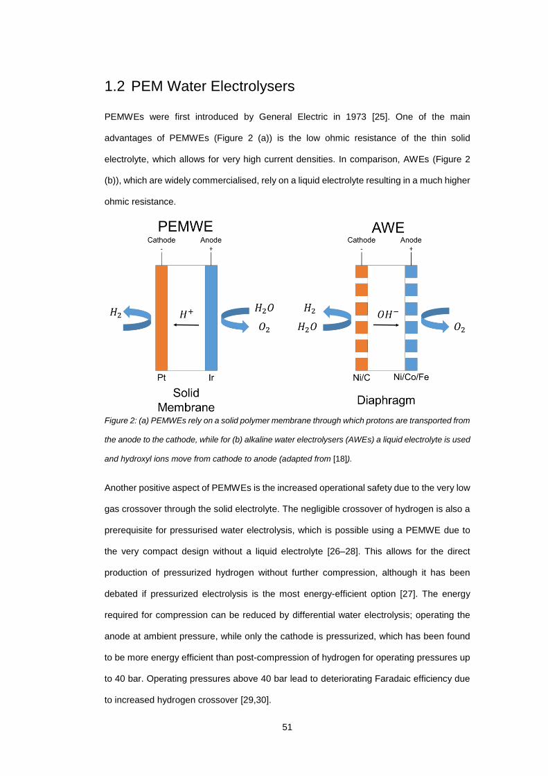
1.2 PEM Water Electrolysers
PEMWEs were first introduced by General Electric in 1973 [25]. One of the main
advantages of PEMWEs (Figure 2 (a)) is the low ohmic resistance of the thin solid
electrolyte, which allows for very high current densities. In comparison, AWEs (Figure 2
(b)), which are widely commercialised, rely on a liquid electrolyte resulting in a much higher
ohmic resistance.
Figure 2: (a) PEMWEs rely on a solid polymer membrane through which protons are transported from
the anode to the cathode, while for (b) alkaline water electrolysers (AWEs) a liquid electrolyte is used
and hydroxyl ions move from cathode to anode (adapted from [18]).
Another positive aspect of PEMWEs is the increased operational safety due to the very low
gas crossover through the solid electrolyte. The negligible crossover of hydrogen is also a
prerequisite for pressurised water electrolysis, which is possible using a PEMWE due to
the very compact design without a liquid electrolyte [26–28]. This allows for the direct
production of pressurized hydrogen without further compression, although it has been
debated if pressurized electrolysis is the most energy-efficient option [27]. The energy
required for compression can be reduced by differential water electrolysis; operating the
anode at ambient pressure, while only the cathode is pressurized, which has been found
to be more energy efficient than post-compression of hydrogen for operating pressures up
to 40 bar. Operating pressures above 40 bar lead to deteriorating Faradaic efficiency due
to increased hydrogen crossover [29,30].
52
The main disadvantage related to PEM water electrolysis are the very high stack costs due
to expensive catalyst, liquid-gas diffusion layer and flow-field materials. On the PEMWE
anode a very corrosive environment, with 𝑝𝐻 ≈ 2 and high potentials above 2 V, is
found [18], which not many materials can withstand. Among these titanium is the most
commonly used at the anode for liquid-gas diffusion layer and flow-fields. Even though
titanium has a much higher corrosion resistance compared to less frequently used
materials like graphite and stainless steel, it is far more expensive and still causes a
PEMWE performance degradation over time as an oxide layer is forming [31]. This can
potentially be overcome by coating with nickel [32], gold, or silver [31], but long term studies
on the stability of these configurations are missing.
Due to the high stack costs for PEMWEs, AWEs are still the industrially dominant
electrolysis technology. However, due to the principal advantages of PEMWEs over AWEs
and the projected cost reductions (see Section 1.1), PEMWEs are likely to play a significant
role for industrial hydrogen production and grid stabilisation. In order to achieve the
technological improvements necessary to drive the uptake of PEMWEs for these real-world
applications, systematic testing of small, lab-scale, single-cell systems is the preferred
mode of research. It allows for rapid testing of new materials and design approaches at
moderate costs and reduced complexity compared to large stacks or systems.
Resulting from the current state-of-the-art and future requirements for PEMWE technology,
a number of key challenges for further development can be identified:
Reduction of catalyst loading, e.g. through novel engineering approaches [33] or
careful analysis of the required catalyst amount [34].
Substitution of noble metal catalysts with low-cost earth-abundant materials, e.g.
nickel- or cobalt-based electrocatalysts [35].
Discovery of novel membrane materials, such as fluorine-free hydrocarbons, to
lower cost and reduce operational voltage to 1.8 V at 3.5 A cm-2 [36].
Improvement of lifetime beyond 20000 h and reduction of degradation rate below
14 µV h-1 [18].
Reduction or replacement of titanium as the primary material for current collectors
and flow-plates.

53
Reduction of the concentration overpotential at high current densities (beyond
2 A cm-2).
54
1.3 Mass Transport Limitations in PEMWEs
A number of effects contribute to the PEMWE operational voltage, which should be as low
as possible to minimise energy consumption. Among these contributions, the concentration
(or mass transport) overpotential is the least known, well-defined, and understood. Even
though the exact definition of the concentration overpotential varies slightly [37–39], it can
be described as the portion of the overall PEMWE voltage which is caused by mass
transport processes and the subsequent lack of reactants or product removal.
The analysis and diagnosis of the concentration overpotential is usually focussed on the
anode, as the mass transport processes here are more complex than at the cathode. Water
has to be transported through the liquid-gas diffusion layer (LGDL) towards the catalyst
layer, where oxygen is produced and subsequently has to be removed from the LGDL into
the flow channels. This concurrent flow of water and oxygen occurs in the pores of the
LGDL, which are limited in size and number, with tortuous pathways, and often only
connected by narrow throats. As the current density increases, the amount of water and
oxygen to be transported scales accordingly, and it becomes increasingly challenging to
ensure sufficient mass transport through the LGDL. Hence, the mass transport contribution
to the overall PEMWE overpotential increases with current density.
However, other processes are believed to contribute to the concentration overpotential.
The two-phase flow in the anode flow-field is widely believed to affect the PEMWE
performance due to blockage effects or shearing of gas bubbles from the LGDL surface
[40–45]. Further, cathode processes can contribute to the concentration overpotential;
however, as water is not usually circulated through the cathode in commercial plants and
the gas diffusion layer is much thinner than the LGDL at the anode, these effects are likely
to be less significant.
55
1.4 Research Motivation
The goal of this thesis is to provide new insight and a suite of low-cost diagnostic tools for
mass transport processes in PEMWEs, particularly enabling improved rates of water and
gas transport at the anode of a PEMWE; hence improving efficiency at high current
densities. The significance of mass transport processes to PEMWE operational voltage will
be outlined in Section 2.3 and the relevant mass transport mechanisms and PEMWE
components will be discussed in the Sections 3.2 and 3.3.
As the issues around climate change and the establishing of renewables as the default
option for energy production become ever more pressing, PEMWEs are likely to be widely
used for hydrogen production and grid stabilisation. This renewed interest in PEMWEs has
caused the technology to mature and the attainable current density to increase. At high
current densities, the mass transport overpotential increasingly contributes to the overall
PEMWE voltage and power requirement, reducing the overall efficiency of hydrogen
production.
As outlined above, the causes and mechanisms of the mass transport overpotential are not
well understood, with significant questions remaining around the exact causes leading to
an increase in overpotential and potential improvements to PEMWE design mitigating mass
transport limitations.
This work aims at gaining insight into the mass transport processes in the anode LGDL and
flow-fields and developing a set of novel diagnostic tools. Due to the high and selective
attenuation of neutrons in water, neutron imaging will be used for measurements of the
LGDL through-plane water thickness and analysed with a focus on mass transport
processes. The neutron imaging data will be combined with X-ray micro-tomography of
LGDL materials to gain an improved understanding of mass transport in the LGDL. These
radiation-based imaging methods will form a benchmark for the low-cost acoustic
diagnostic tools used in this work. Two different acoustic techniques, acoustic emission
and acoustic time-of-flight imaging, will be used to investigate mass transport in the
PEMWE flow channels and LGDL and the results validated against established techniques
and calculations. These acoustic diagnostic techniques have not been previously applied
56
to PEMWEs, and with one exception not to AWEs either [46]. By combining insights from
this suite of techniques it is expected to develop an understanding of the effects in LGDL
and flow channels contributing to the mass transport overpotential. Further, this work is
expected to establish the aforementioned low-cost diagnostic techniques in the PEMWE
field; hence, accelerating future work on mass transport limitations in PEMWEs and
contributing to the development of new materials and novel engineering approaches to
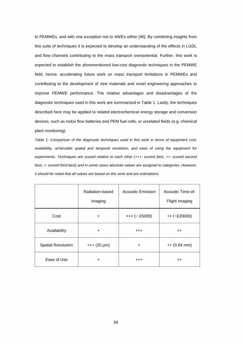
improve PEMWE performance. The relative advantages and disadvantages of the
diagnostic techniques used in this work are summarized in Table 1. Lastly, the techniques
described here may be applied to related electrochemical energy storage and conversion
devices, such as redox flow batteries and PEM fuel cells, or unrelated fields (e.g. chemical
plant monitoring).
Table 1: Comparison of the diagnostic techniques used in this work in terms of equipment cost,
availability, achievable spatial and temporal resolution, and ease of using the equipment for
experiments. Techniques are scored relative to each other (+++: scored best, ++: scored second
best, +: scored third best) and in some cases absolute values are assigned to categories. However,
it should be noted that all values are based on this work and are estimations.
Radiation-based
Imaging
Acoustic Emission Acoustic Time-of-
Flight Imaging
Cost + +++ (~ £5000) ++ (~£20000)
Availability + +++ ++
Spatial Resolution +++ (20 µm) + ++ (0.94 mm)
Ease of Use + +++ ++
57
1.5 Thesis Overview
This introduction will be followed by a short discussion of the fundamental aspects of
PEMWE assembly and sources of voltage loss in a PEMWE, which are necessary to
facilitate understanding of this work. PEMWE electrocatalysts and membrane materials are
not within the scope of this thesis, but a short summary will be given on state-of-the-art
materials.
Subsequently, the scientific literature on the PEMWE components most relevant to this
work, the liquid-gas diffusion layer (LGDL) and the flow-fields, will be reviewed, and existing
materials and designs will be discussed. A particular focus will be placed on mass transport
aspects. The literature review will end with a discussion of the existing body of literature on
PEMWE diagnostic tools – the most common techniques as well as the novel tools
introduced in this work.
A detailed discussion of the experimental methodology employed in this work will begin
with details on the operation and assembly of PEMWE cells. This will be followed by the
scientific foundations of X-ray and neutron imaging, the elementary methodology of image
analysis and tomographic reconstruction, and the underlying mechanisms of acoustic
processes.
The main results section is separated into three main chapters: results on the influence of
LGDL microstructure on the water-gas distribution in the LGDL obtained with neutron
imaging, followed by diagnosis of the flow regime in the flow channels using acoustic
emission, the use of acoustic time-of-flight imaging to monitor the flow regime in the flow
channels, as well as the water-gas distribution in the LGDL. Each chapter will end with a
conclusion, outlining the significance of the results and their implications on the
optimisation of PEMWE design.
This thesis will be concluded by a summary of the presented work and a number of potential
directions for future work, based on the results obtained. This includes novel engineering
approaches mitigating the drawbacks of existing LGDLs, and the use of acoustic
techniques in conjunction with radiation-based imaging techniques (e.g. neutron imaging).

59
2 Fundamentals of PEMWE Operation


61
2.1 Overview
This chapter will briefly review the fundamental knowledge necessary for understanding
the following sections. The assembly of PEMWE cells from individual components will be
introduced, followed by a discussion of voltage losses in a PEMWE, with a focus on the
mass transport overpotential. Lastly, the electrocatalysts used at anode and cathode and
the membrane material will be discussed briefly.
62
2.2 PEMWE Cell Assembly
Figure 3 shows the assembly of a typical PEMWE with the catalyst coated membrane
(CCM), the liquid-gas diffusion layer (LGDL) at the anode, the gas diffusion layer (GDL) at
the cathode, flow-fields, and end-plates. The end-plates are usually relatively thick (2 cm
or more), which minimizes bowing of the end-plates and avoids breaking of brittle end-plate
materials, such as acrylic. The flow-plates typically have a current collector tab, which
allows for easy mounting of the power supply terminals. Gaskets (not displayed) are usually
employed to keep LGDL, GDL, and CCM in place and to prevent leakage. The use of a
CCM is the most commonly used approach, but it is possible to apply the catalysts to the
surface of the LGDL/GDL and combine these with an uncoated ionomer membrane. This
yields an equivalent sequence of functional layers and has been shown to produce
comparable performance [47,48].
The single-cell PEMWE shown here is typically used for research work and is well-suited
to demonstrate the basic processes and function of a PEMWE. However, for commercial
applications PEMWE stacks are used, that combine multiple single cells into one unit [49],
but are subject to the same processes discussed in this work.
The nomenclature used in this work for LGDL and GDL was chosen as it best describes
the movement of water and gas in the respective components. However, a variety of terms
are used across the scientific literature, with the anode LGDL often described as the porous
transport layer (PTL) or, in analogy to PEM fuel cells, as the gas diffusion layer (GDL).
63
Figure 3: (a) The assembly of a single-cell PEMWE with end-plates, flow-fields, liquid-gas diffusion
layer (LGDL), gas diffusion layer (GDL), and catalyst coated membrane (CCM). (b) Water reacts at
the catalyst layer (CL) on the anode side. Oxygen is transported back to the flow channels through
the LGDL, while protons migrate through the membrane and electrons through the outer circuit to the
cathode side. These react at the cathode CL to form hydrogen. Water circulation at the cathode is
not strictly necessary, but is often used to facilitate hydration (indicated by brackets).
64
Water enters the PEMWE through the end-plate on the anode side and is transported
across the active area along the channels of the flow-field. The water then crosses through
the porous LGDL towards the anode catalyst layer (CL), where it is oxidised to form
protons, electrons and molecular oxygen. The protons are transported through the
membrane to the cathode CL, where hydrogen is formed. However, the oxygen has to be
transported from the anode CL, through the LGDL, back to the flow channels where it is
carried out of the PEMWE cell with the unreacted water. While crossing the LGDL, the
oxygen gas is in counter-current flow to the water traveling from the flow-field to the catalyst
layer. Even though it is not strictly necessary for the operation of a PEMWE, water is often
circulated through the cathode side as well to ensure sufficient hydration of the membrane,
which reduces its ohmic resistance and facilitates proton transport through the membrane.
The use of a solid electrolyte allows for a compact build with a minimum amount of liquid
in the PEMWE cell. Nevertheless, the costs of a PEMWE stack still amount to a significant
proportion of the overall system, with indicative reports quoting 37 % of the total costs of a
plant [50]. Innovation in stack design and manufacture is reducing costs and improving
durability and efficiency. For example, Chisholm et al. [31] 3D printed and silver-coated
PEMWE flow plates from polypropylene. These flow plates were ~4 times lighter and 5
times cheaper than conventional plates from titanium and showed a voltage degradation
rate of only 0.14 mV h-1 over 100 hours at 0.25 A cm-2. Another approach to use additive
manufacturing for PEMWE parts was taken by Yang et al. [51], who used selective laser
melting to create a multifunctional plate incorporating LGDL, gasket, flow-plate and end-
plate.
65
2.3 Sources of Voltage Loss in a PEMWE
The decomposition of water is driven by heat and electrical energy. The minimum electrical
energy required for the decomposition of water is the reversible voltage V𝑟𝑒𝑣 = 1.23 𝑉, while
the thermoneutral voltage V𝑡𝑛 = 1.48 𝑉 is required if no external heat is supplied [27].
V𝑟𝑒𝑣 is the minimum thermodynamic potential necessary to drive the water-splitting reaction
at standard conditions. However, several other voltage contributions have to be accounted
for, which constitute the operational voltage 𝑉 [37,38,52].
V = V𝑜𝑐 + V𝑎𝑐𝑡 + V𝑜ℎ𝑚 + V𝑐𝑜𝑛 (Equation 2-1)
Here, V𝑜𝑐 is the open-circuit voltage, which depends on the reversible voltage V𝑟𝑒𝑣 and the
activities 𝑎 of reactants and products [38,52,53]:
V𝑜𝑐 = Vrev + 𝑅𝑇
2𝐹 ln (
𝑎𝐻2√𝑎𝑂2
𝑎𝐻2𝑂) . (Equation 2-2)
𝑇 denotes the temperature, 𝑅 is the universal gas constant, and 𝐹 is the Faraday constant.
The activity of liquid water is 1.
V𝑎𝑐𝑡 is the activation overpotential, which is associated with the activation energy of the
water electrolysis reactions and can be described by the Butler-Volmer equation. The
equation given here is most commonly used in the literature [18,37,38,53–56]; however,
the use of the Butler-Volmer equation for multi-electron reactions as occurring in PEMWEs
has been questioned [57].
V𝑎𝑐𝑡 = V𝑎𝑐𝑡,𝑎𝑛 + 𝑉𝑎𝑐𝑡,𝑐𝑎𝑡 (Equation 2-3)
V𝑎𝑐𝑡 =𝑅𝑇
𝛼𝑎𝑛𝐹sinh−1 (
𝑖
2𝑖0,𝑎𝑛) +
𝑅𝑇
𝛼𝑐𝑎𝑡𝐹sinh−1 (
𝑖
2𝑖0,𝑐𝑎𝑡) (Equation 2-4)
Anode and cathode contributions are denoted by 𝑎𝑛 and 𝑐𝑎𝑡, respectively. Typical values
for the charge transfer coefficients are 𝛼𝑎𝑛 = 2 and 𝛼𝑐𝑎𝑡 = 0.5 [18]. The exchange current
density is denoted by 𝑖0. The current density 𝑖 is the current 𝐼 normalized by the geometric
active area 𝐴 of the PEMWE.
The exchange current density is calculated from the activation energy 𝐸𝐴 at the respective
electrode and a reference value 𝑖0,𝑟𝑒𝑓 which is obtained from literature or fitting
experimental polarisation data [58]:
66
𝑖0 = 𝑖0,𝑟𝑒𝑓𝑒𝑥𝑝 (−𝐸𝐴
𝑅(
1
𝑇−
1
𝑇𝑟𝑒𝑓)) (Equation 2-5)
The activation overpotential represents the kinetic characteristics of the electrode
processes, and as such can be significantly influenced by electrode and catalyst
microstructure and morphology. A more detailed discussion of electrode kinetics and the
use of the Butler-Volmer equation for water electrolysis can be found elsewhere [57].
The ohmic overpotential 𝑉𝑜ℎ𝑚 is caused by the ohmic resistance 𝑅 of the different parts of
the PEMWE, which consists of flow-plates, 𝑓𝑝, liquid-gas diffusion layers, 𝑙𝑔𝑑𝑙 and the
catalyst coated membrane, 𝑐𝑐𝑚 [38,39,52]:
𝑉𝑜ℎ𝑚 = 𝑅𝐼 = (𝑅𝑓𝑝 + 𝑅𝑙𝑔𝑑𝑙 + 𝑅𝑐𝑐𝑚)𝐼 . (Equation 2-6)
The ohmic resistances above contain a portion that is attributed to the contact resistance
between the respective part and the adjacent PEMWE component. This contact resistance
can contribute significantly to the overall PEMWE overpotential [51] and is typically
calculated from electrochemical impedance spectroscopy results [59]. Further, if the ohmic
overpotential of a PEMWE stack is calculated, the ohmic resistance of the bipolar plates
has to be accounted for.
The concentration overpotential 𝑉𝑐𝑜𝑛 is caused by limitations in the supply of reactant or the
blockage of active catalyst sites by an excess of product. This occurs in particular at high
current densities when high flow rates of water are required, and large amounts of oxygen
and hydrogen are produced. From the inlet, water is transported through the flow channels
and has to cross the porous LGDL to reach the active catalyst sites on the surface of the
membrane. Simultaneously, the product gas is produced at the CCM and needs to move
through the LGDL in counter-current flow to the water. As the mass flow through the LGDL
is increasingly inhibited by the increasing amount of water and gas, additional energy is
required to overcome this resistance. To provide this excess energy, an increased voltage
has to be supplied to the PEMWE, which is the concentration overpotential.
The concentration overpotential is modelled as a logarithmic increase for product (𝑂2, 𝐻2)
concentrations at the membrane 𝑚𝑒 exceeding the concentrations at a reference state 0.
This definition was introduced for PEMWEs by Marangio et al. [37] and has been followed
by the vast majority of publications [38,39,52,53,55,60,61].
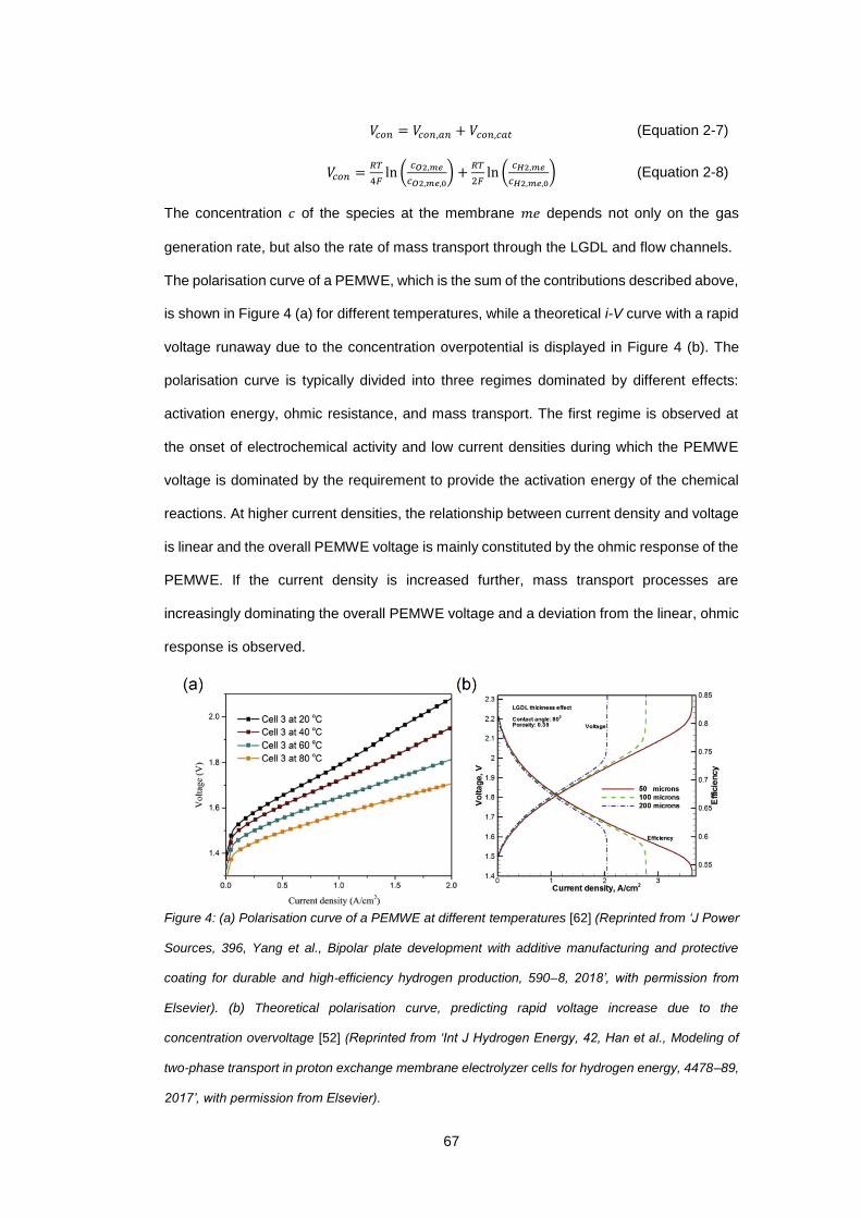
67
𝑉𝑐𝑜𝑛 = 𝑉𝑐𝑜𝑛,𝑎𝑛 + 𝑉𝑐𝑜𝑛,𝑐𝑎𝑡 (Equation 2-7)
𝑉𝑐𝑜𝑛 =𝑅𝑇
4𝐹ln (
𝑐𝑂2,𝑚𝑒
𝑐𝑂2,𝑚𝑒,0) +
𝑅𝑇
2𝐹ln (
𝑐𝐻2,𝑚𝑒
𝑐𝐻2,𝑚𝑒,0) (Equation 2-8)
The concentration 𝑐 of the species at the membrane 𝑚𝑒 depends not only on the gas
generation rate, but also the rate of mass transport through the LGDL and flow channels.
The polarisation curve of a PEMWE, which is the sum of the contributions described above,
is shown in Figure 4 (a) for different temperatures, while a theoretical i-V curve with a rapid
voltage runaway due to the concentration overpotential is displayed in Figure 4 (b). The
polarisation curve is typically divided into three regimes dominated by different effects:
activation energy, ohmic resistance, and mass transport. The first regime is observed at
the onset of electrochemical activity and low current densities during which the PEMWE
voltage is dominated by the requirement to provide the activation energy of the chemical
reactions. At higher current densities, the relationship between current density and voltage
is linear and the overall PEMWE voltage is mainly constituted by the ohmic response of the
PEMWE. If the current density is increased further, mass transport processes are
increasingly dominating the overall PEMWE voltage and a deviation from the linear, ohmic
response is observed.
Figure 4: (a) Polarisation curve of a PEMWE at different temperatures [62] (Reprinted from ‘J Power
Sources, 396, Yang et al., Bipolar plate development with additive manufacturing and protective
coating for durable and high-efficiency hydrogen production, 590–8, 2018’, with permission from
Elsevier). (b) Theoretical polarisation curve, predicting rapid voltage increase due to the
concentration overvoltage [52] (Reprinted from ‘Int J Hydrogen Energy, 42, Han et al., Modeling of
two-phase transport in proton exchange membrane electrolyzer cells for hydrogen energy, 4478–89,
2017’, with permission from Elsevier).
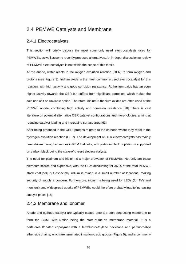
68
2.4 PEMWE Catalysts and Membrane
2.4.1 Electrocatalysts
This section will briefly discuss the most commonly used electrocatalysts used for
PEMWEs, as well as some recently proposed alternatives. An in-depth discussion or review
of PEMWE electrocatalysts is not within the scope of this thesis.
At the anode, water reacts in the oxygen evolution reaction (OER) to form oxygen and
protons (see Figure 3). Iridium oxide is the most commonly used electrocatalyst for this
reaction, with high activity and good corrosion resistance. Ruthenium oxide has an even
higher activity towards the OER but suffers from significant corrosion, which makes the
sole use of it an unviable option. Therefore, iridium/ruthenium oxides are often used at the
PEMWE anode, combining high activity and corrosion resistance [18]. There is vast
literature on potential alternative OER catalyst configurations and morphologies, aiming at
reducing catalyst loading and increasing surface area [63].
After being produced in the OER, protons migrate to the cathode where they react in the
hydrogen evolution reaction (HER). The development of HER electrocatalysts has mainly
been driven through advances in PEM fuel cells, with platinum black or platinum supported
on carbon black being the state-of-the-art electrocatalysts.
The need for platinum and iridium is a major drawback of PEMWEs. Not only are these
elements scarce and expensive, with the CCM accounting for 36 % of the total PEMWE
stack cost [50], but especially iridium is mined in a small number of locations, making
security of supply a concern. Furthermore, iridium is being used for LEDs (for TVs and
monitors), and widespread uptake of PEMWEs would therefore probably lead to increasing
catalyst prices [18].
2.4.2 Membrane and Ionomer
Anode and cathode catalyst are typically coated onto a proton-conducting membrane to
form the CCM, with Nafion being the state-of-the-art membrane material. It is a
perfluorosulfonated copolymer with a tetrafluoroethylene backbone and perfluoroalkyl
ether side chains, which are terminated in sulfonic acid groups (Figure 5), and is commonly
69
deployed in thicknesses of 0.007 inch (~0.18 mm, Nafion 117) or 0.005 inch (~0.13 mm,
Nafion 115) [64].
Nafion is also commonly mixed into the catalyst layers as an ionomer, which enhances
proton conductivity from the catalyst layer to the membrane and provides a support
structure for the catalysts, hence acting as a binder. The ionomer loading typically ranges
between 20 wt% and 30 wt% of the catalyst [18].
Figure 5: Chemical structure of Nafion, consisting of a tetrafluoroethylene backbone and side chains
carrying a sulfonic acid group [64]. (Reprinted with permission from Mauritz KA, Moore RB. Chem
Rev. 104:4535–85. Copyright (2004) American Chemical Society.)


71
3 Literature Review

73
3.1 Overview
This chapter will review and discuss the scientific literature relevant to mass transport in
PEMWEs. The review will begin with an outline of the mass flux in PEMWE flow-fields, the
different flow regimes found, and the design of flow-field geometries. This will be followed
by a discussion of typical LGDL materials; their structure, properties, as well as use in
PEMWEs. The review will end with a summary of the diagnostic techniques used to
investigate mass transport aspects in PEMWEs. The work in this chapter has been
submitted to the International Journal of Hydrogen Energy.
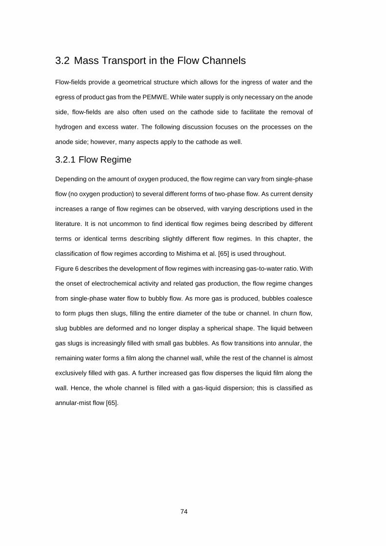
74
3.2 Mass Transport in the Flow Channels
Flow-fields provide a geometrical structure which allows for the ingress of water and the
egress of product gas from the PEMWE. While water supply is only necessary on the anode
side, flow-fields are also often used on the cathode side to facilitate the removal of
hydrogen and excess water. The following discussion focuses on the processes on the
anode side; however, many aspects apply to the cathode as well.
3.2.1 Flow Regime
Depending on the amount of oxygen produced, the flow regime can vary from single-phase
flow (no oxygen production) to several different forms of two-phase flow. As current density
increases a range of flow regimes can be observed, with varying descriptions used in the
literature. It is not uncommon to find identical flow regimes being described by different
terms or identical terms describing slightly different flow regimes. In this chapter, the
classification of flow regimes according to Mishima et al. [65] is used throughout.
Figure 6 describes the development of flow regimes with increasing gas-to-water ratio. With
the onset of electrochemical activity and related gas production, the flow regime changes
from single-phase water flow to bubbly flow. As more gas is produced, bubbles coalesce
to form plugs then slugs, filling the entire diameter of the tube or channel. In churn flow,
slug bubbles are deformed and no longer display a spherical shape. The liquid between
gas slugs is increasingly filled with small gas bubbles. As flow transitions into annular, the
remaining water forms a film along the channel wall, while the rest of the channel is almost
exclusively filled with gas. A further increased gas flow disperses the liquid film along the
wall. Hence, the whole channel is filled with a gas-liquid dispersion; this is classified as
annular-mist flow [65].
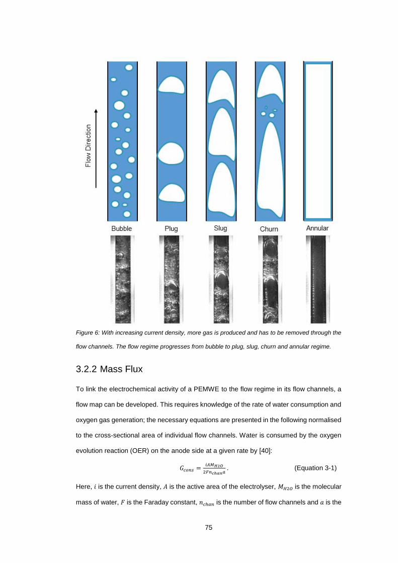
75
Figure 6: With increasing current density, more gas is produced and has to be removed through the
flow channels. The flow regime progresses from bubble to plug, slug, churn and annular regime.
3.2.2 Mass Flux
To link the electrochemical activity of a PEMWE to the flow regime in its flow channels, a
flow map can be developed. This requires knowledge of the rate of water consumption and
oxygen gas generation; the necessary equations are presented in the following normalised
to the cross-sectional area of individual flow channels. Water is consumed by the oxygen
evolution reaction (OER) on the anode side at a given rate by [40]:
𝐺𝑐𝑜𝑛𝑠 =𝑖𝐴𝑀𝐻2𝑂
2𝐹𝑛𝑐ℎ𝑎𝑛𝑎 . (Equation 3-1)
Here, 𝑖 is the current density, 𝐴 is the active area of the electrolyser, 𝑀𝐻2𝑂 is the molecular
mass of water, 𝐹 is the Faraday constant, 𝑛𝑐ℎ𝑎𝑛 is the number of flow channels and 𝑎 is the
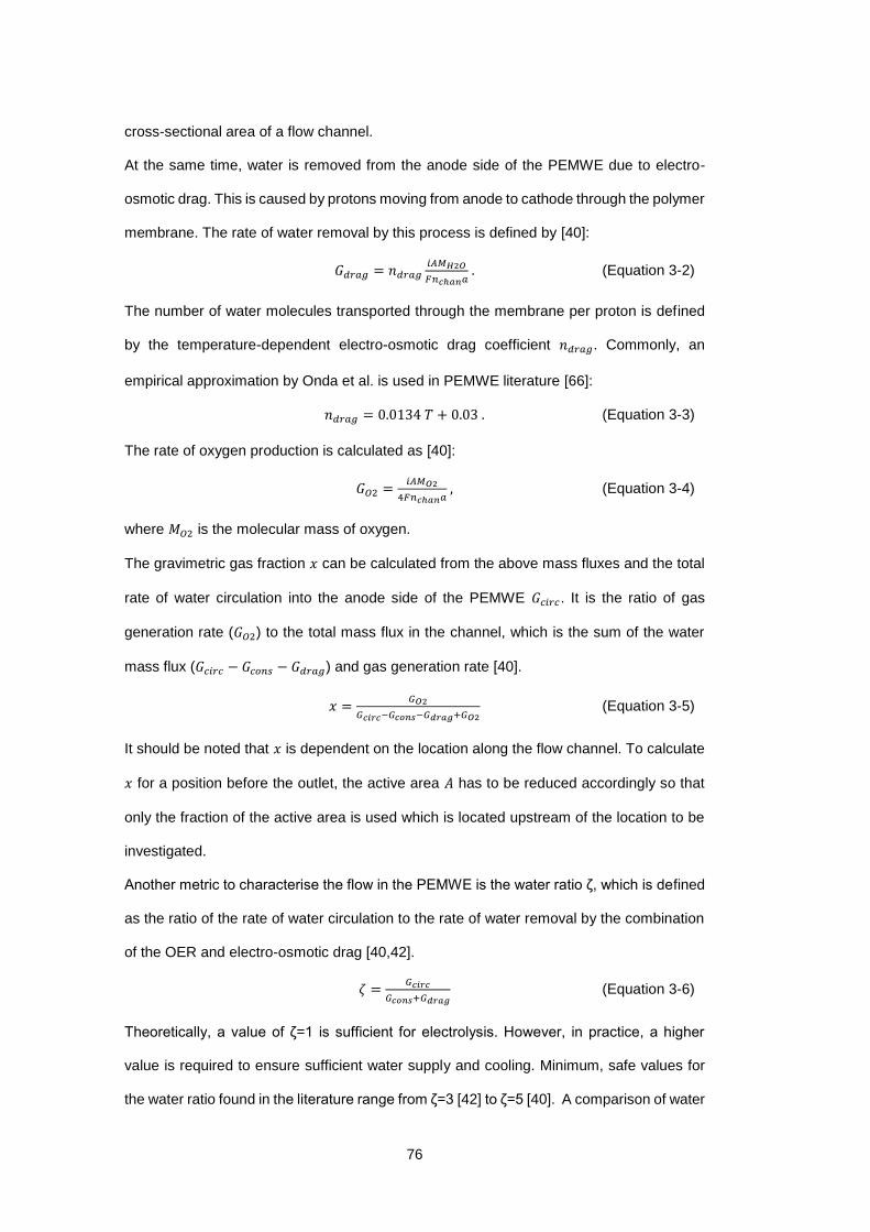
76
cross-sectional area of a flow channel.
At the same time, water is removed from the anode side of the PEMWE due to electro-
osmotic drag. This is caused by protons moving from anode to cathode through the polymer
membrane. The rate of water removal by this process is defined by [40]:
𝐺𝑑𝑟𝑎𝑔 = 𝑛𝑑𝑟𝑎𝑔𝑖𝐴𝑀𝐻2𝑂
𝐹𝑛𝑐ℎ𝑎𝑛𝑎 . (Equation 3-2)
The number of water molecules transported through the membrane per proton is defined
by the temperature-dependent electro-osmotic drag coefficient 𝑛𝑑𝑟𝑎𝑔. Commonly, an
empirical approximation by Onda et al. is used in PEMWE literature [66]:
𝑛𝑑𝑟𝑎𝑔 = 0.0134 𝑇 + 0.03 . (Equation 3-3)
The rate of oxygen production is calculated as [40]:
𝐺𝑂2 =𝑖𝐴𝑀𝑂2
4𝐹𝑛𝑐ℎ𝑎𝑛𝑎 , (Equation 3-4)
where 𝑀𝑂2 is the molecular mass of oxygen.
The gravimetric gas fraction 𝑥 can be calculated from the above mass fluxes and the total
rate of water circulation into the anode side of the PEMWE 𝐺𝑐𝑖𝑟𝑐. It is the ratio of gas
generation rate (𝐺𝑂2) to the total mass flux in the channel, which is the sum of the water
mass flux (𝐺𝑐𝑖𝑟𝑐 − 𝐺𝑐𝑜𝑛𝑠 − 𝐺𝑑𝑟𝑎𝑔) and gas generation rate [40].
𝑥 =𝐺𝑂2
𝐺𝑐𝑖𝑟𝑐−𝐺𝑐𝑜𝑛𝑠−𝐺𝑑𝑟𝑎𝑔+𝐺𝑂2 (Equation 3-5)
It should be noted that 𝑥 is dependent on the location along the flow channel. To calculate
𝑥 for a position before the outlet, the active area 𝐴 has to be reduced accordingly so that
only the fraction of the active area is used which is located upstream of the location to be
investigated.
Another metric to characterise the flow in the PEMWE is the water ratio ζ, which is defined
as the ratio of the rate of water circulation to the rate of water removal by the combination
of the OER and electro-osmotic drag [40,42].
휁 =𝐺𝑐𝑖𝑟𝑐
𝐺𝑐𝑜𝑛𝑠+𝐺𝑑𝑟𝑎𝑔 (Equation 3-6)
Theoretically, a value of ζ=1 is sufficient for electrolysis. However, in practice, a higher
value is required to ensure sufficient water supply and cooling. Minimum, safe values for
the water ratio found in the literature range from ζ=3 [42] to ζ=5 [40]. A comparison of water
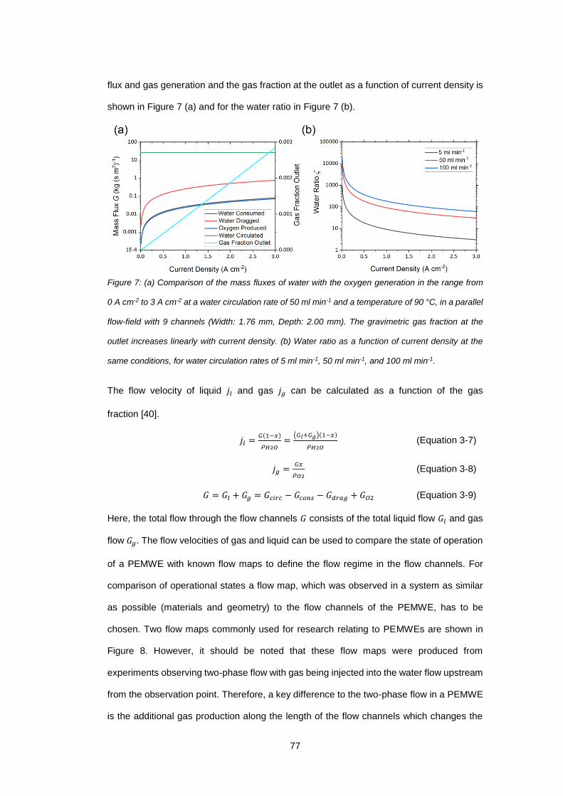
77
flux and gas generation and the gas fraction at the outlet as a function of current density is
shown in Figure 7 (a) and for the water ratio in Figure 7 (b).
Figure 7: (a) Comparison of the mass fluxes of water with the oxygen generation in the range from
0 A cm-2 to 3 A cm-2 at a water circulation rate of 50 ml min-1 and a temperature of 90 °C, in a parallel
flow-field with 9 channels (Width: 1.76 mm, Depth: 2.00 mm). The gravimetric gas fraction at the
outlet increases linearly with current density. (b) Water ratio as a function of current density at the
same conditions, for water circulation rates of 5 ml min-1, 50 ml min-1, and 100 ml min-1.
The flow velocity of liquid 𝑗𝑙 and gas 𝑗𝑔 can be calculated as a function of the gas
fraction [40].
𝑗𝑙 =𝐺(1−𝑥)
𝜌𝐻2𝑂=
(𝐺𝑙+𝐺𝑔)(1−𝑥)
𝜌𝐻2𝑂 (Equation 3-7)
𝑗𝑔 =𝐺𝑥
𝜌𝑂2 (Equation 3-8)
𝐺 = 𝐺𝑙 + 𝐺𝑔 = 𝐺𝑐𝑖𝑟𝑐 − 𝐺𝑐𝑜𝑛𝑠 − 𝐺𝑑𝑟𝑎𝑔 + 𝐺𝑂2 (Equation 3-9)
Here, the total flow through the flow channels 𝐺 consists of the total liquid flow 𝐺𝑙 and gas
flow 𝐺𝑔. The flow velocities of gas and liquid can be used to compare the state of operation
of a PEMWE with known flow maps to define the flow regime in the flow channels. For
comparison of operational states a flow map, which was observed in a system as similar
as possible (materials and geometry) to the flow channels of the PEMWE, has to be
chosen. Two flow maps commonly used for research relating to PEMWEs are shown in
Figure 8. However, it should be noted that these flow maps were produced from
experiments observing two-phase flow with gas being injected into the water flow upstream
from the observation point. Therefore, a key difference to the two-phase flow in a PEMWE
is the additional gas production along the length of the flow channels which changes the
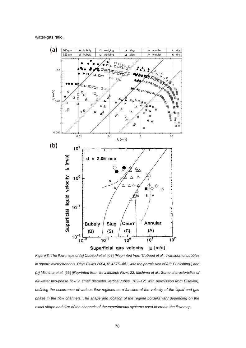
78
water-gas ratio.
Figure 8: The flow maps of (a) Cubaud et al. [67] (Reprinted from ‘Cubaud et al., Transport of bubbles
in square microchannels. Phys Fluids 2004;16:4575–85.’, with the permission of AIP Publishing.) and
(b) Mishima et al. [65] (Reprinted from ‘Int J Multiph Flow, 22, Mishima et al., Some characteristics of
air-water two-phase flow in small diameter vertical tubes, 703–12’, with permission from Elsevier),
defining the occurrence of various flow regimes as a function of the velocity of the liquid and gas
phase in the flow channels. The shape and location of the regime borders vary depending on the
exact shape and size of the channels of the experimental systems used to create the flow map.
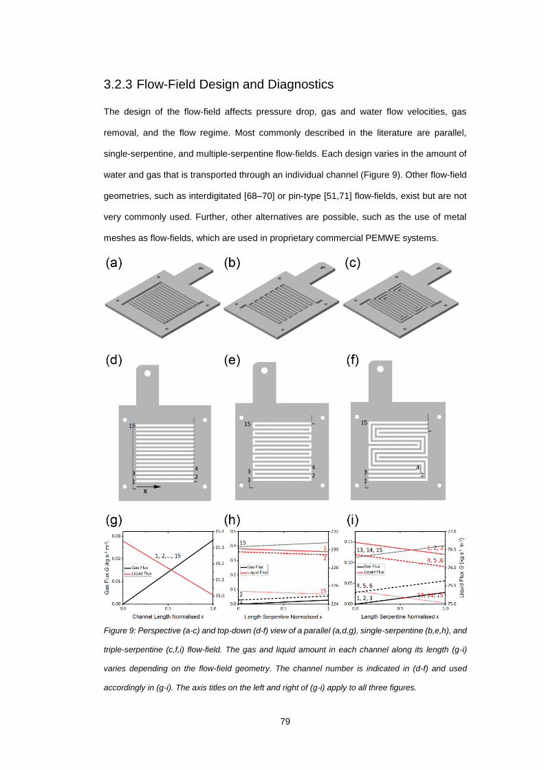
79
3.2.3 Flow-Field Design and Diagnostics
The design of the flow-field affects pressure drop, gas and water flow velocities, gas
removal, and the flow regime. Most commonly described in the literature are parallel,
single-serpentine, and multiple-serpentine flow-fields. Each design varies in the amount of
water and gas that is transported through an individual channel (Figure 9). Other flow-field
geometries, such as interdigitated [68–70] or pin-type [51,71] flow-fields, exist but are not
very commonly used. Further, other alternatives are possible, such as the use of metal
meshes as flow-fields, which are used in proprietary commercial PEMWE systems.
Figure 9: Perspective (a-c) and top-down (d-f) view of a parallel (a,d,g), single-serpentine (b,e,h), and
triple-serpentine (c,f,i) flow-field. The gas and liquid amount in each channel along its length (g-i)
varies depending on the flow-field geometry. The channel number is indicated in (d-f) and used
accordingly in (g-i). The axis titles on the left and right of (g-i) apply to all three figures.
80
In parallel flow-fields (Figure 9 (a),(d),(g)), the flow is separated into a number of separate
channels, which are connected by a dividing and a combining manifold. Ideally, the amount
of water and gas passing through an individual channel is the corresponding fraction of the
total amount of water and gas with respect to the total number of channels, however, a
non-uniform distribution of flow occurs [72]. For a single-serpentine flow-field (Figure 9
(b),(e),(h)), all of the water and gas has to pass through one channel, thus causing much
higher flow velocities than in a parallel flow-field. Hence, the pressure drop in a single-
serpentine flow-field is significantly higher than for a parallel flow-field [40].
There is conflicting information on the performance of these flow-fields. Ito et al. [40]
showed improved performance of a PEMWE (active area: 5.2 × 5.2 cm) with a parallel flow-
field up to 1 A cm-2. They assigned this difference in performance to an increased
concentration overpotential in the single-serpentine flow-field. However, it is unlikely that
this effect is notable at current densities as low as 1 A cm-2. Majasan et al. [73] also found
improved performance for the parallel flow-field for current densities of up to 3 A cm-2,
whereas, Li et al. [74] showed superior performance of a single-serpentine flow-field. In this
study, the parallel flow-field was also shown to have the highest ohmic resistance, which
partly explains the decreased performance. This raises the question if the dominant factors
influencing the electrochemical performance of different flow-fields are flow effects or
simply the ohmic resistance of the flow-plate. In the latter case, further work is necessary
to optimise flow-field geometry by minimising ohmic resistance (channel-to-land ratio) while
ensuring a sufficiently low pressure drop.
Multiple-serpentine flow-fields (Figure 9 (c),(f),(i)) share characteristics of the parallel as
well as the single-serpentine flow-field. Their electrochemical performance and pressure
drop were found to be intermediate to those of parallel and single-serpentine flow-
fields [40].
All flow-fields shown in Figure 9 are of the Z-type, with the inlet and outlet being located at
diagonally opposed sides of the active area (bottom left and top right). Alternatively, flow-
fields can be designed in a U-shape, which would require the inlet and outlet being located
at the same side of the active area (e.g. bottom left and top left). The location of inlet and
outlet has been shown to have a significant impact on the distribution of water flow between
81
individual channels of a flow-field [72,75,76].
There is very little published research examining possibilities to optimise flow-fields beyond
the differentiation of parallel, single and multiple-serpentine designs. Majasan et al. showed
that the performance of a PEMWE is affected by the depth of the flow channels and
demonstrated a varying degree of mass transport limitation with flow channel depth at
different current densities. A non-monotonic trend was found, implying the possibility of
optimising the flow-field design [77].
A multitude of approaches have been deployed to image and diagnose the processes in
the flow channels of PEMWEs. Most publications use either optical, X-ray or neutron
imaging to visualize bubble and water flow. Optical imaging is comparatively low-cost and
easy to implement, which makes it a preferred tool for flow-field diagnosis [33,43,44,78–
82]. X-ray and neutron imaging, on the other hand, are expensive, require large-scale
facilities, and often the PEMWE cell needs to be adapted or miniaturized to facilitate
measurement. However, these techniques offer quantitative capabilities and the possibility
of analysing the processes in the flow-field, LGDL and catalyst layer simultaneously, which
explains the attraction of X-ray [83,84] and neutron imaging [85–90] techniques for the
study of PEMWEs. X-ray imaging usually offers a higher flux and therefore shorter
acquisition times, while the preferential attenuation of neutrons in hydrogen and water
makes neutron imaging an especially valuable diagnostic tool by enhancing the contrast of
these molecules compared to other materials [91].
3.2.4 Influence of the Flow Regime on Performance
There are essentially two opposing model concepts on how the flow regime can affect the
overall performance of a PEMWE. The first idea assumes that the formation of gas slugs
in the flow channel hinders the supply of water to the LGDL, and consequentially to the
catalyst sites. This would then decrease overall performance by amplifying the
concentration overpotential [41]. The second concept assumes that the bubbles in the flow
channel cause turbulence which leads other bubbles in the vicinity to detach from the LGDL
surface. This effect gets stronger when the size of bubbles in the flow channel increases.
Hence, bubbles are effectively removed from the LGDL surface, which accelerates gas
82
removal from the catalyst sites and through the LGDL. This would cause a decrease in
concentration overpotential [44].
Ito et al. [40] measured the performance of a PEMWE, comparing three different flow-field
designs: parallel, single-serpentine, and dual-serpentine. As shown in Section 3.2.3, the
water flow speed, water-to-gas ratio, and flow regime vary widely between these designs
even at identical operating conditions. In particular, flow-fields with fewer flow channels
(serpentine) favour the development of flow regimes with a low water-to-gas ratio (slug,
annular), while flow-fields with multiple channels (parallel) favour flow regimes with a higher
water-to-gas ratio, such as bubbly flow. As the authors observed a decrease in
performance from the parallel to single-serpentine and then dual-serpentine flow-field, they
concluded that performance deteriorates for flow regimes with a lower water-to-gas ratio
than bubbly flow [40].
In later work, Ito et al. [41] examined the occurrence and pressure drop of different flow
regimes and the link between the mean pore diameter of the LGDL and the development
of the flow regime. Their theoretical considerations and experimental data imply that an
LGDL with bigger pores results in a larger bubble detachment diameter and hence plug
and slug flow are reached at lower current densities compared to an LGDL with smaller
pores. This leads to vast areas of the liquid-gas diffusion layer being covered by gas
bubbles, which they postulated had a negative effect on performance. In subsequent work,
the authors [92] measured the cell resistance and overall performance using titanium felts
of different pore size as LGDLs. An increase in cell resistance with increasing pore size
was found, which is attributed to an increase in bubble detachment radius.
Sun et al. [42] performed current mapping and localised electrochemical impedance
spectroscopy (EIS) on a PEMWE under water starvation and showed that in the case of
water starvation, performance decreases under slug and churn flow compared to the
bubble regime. Similar observations of the decrease of local current density towards the
end of the channel (where slug and churn flow preferably occur) under water starvation
have been made by Immerz et al. [93,94]. However, both authors compared subsequent
locations along the flow in a PEMWE and not a whole cell under different regimes.
Therefore, it is uncertain if these results can show the influence of the flow regime properly,
83
as flow regime and water starvation effects occur at the same time.
Using EIS and high-speed imaging, Dedigama et al. [43] came to a contrary conclusion;
their results showed an improvement in mass transport which is associated with the
transition from bubble to slug flow. Further, Dedigama et al. [44] mapped the current density
at different locations along a single-channel PEMWE and found an increase in performance
towards the top end of the channel and showed that slug flow is the dominant flow regime
at this location. This supported the earlier finding that performance is enhanced in slug
flow. However, it has been proposed that this might be caused by an increase in
temperature along the flow channel [95]. Further, the increase in mass transfer inhibition
observed at higher water flow rates (in bubble flow) can be seen as a consequence of the
increased kinetic energy of water flow in the flow channel, which hinders the detachment
of gas bubbles from the LGDL surface into the flow channel [45]. In that case, the
performance effect would be unrelated to the flow regime in the flow channels.
There is a lack of consensus and understanding of the exact relationship between PEMWE
performance and the flow regime. Further, to date, no coherent model of the processes
underlying potential performance changes due to a specific flow regime has been
developed and backed by conclusive experimental data.
3.2.5 Two-Phase Modelling
Modelling of the two-phase flow offers the opportunity to predict the effects of changes to
geometry or physical parameters in a low-cost and rapid way. Only a few publications have
provided comprehensive 3D models incorporating two-phase flow, specifically aiming at
PEMWEs [68,70,96,97]. Lafmejani et al. [70] published a 3D volume-of-fluid model and
qualitatively confirmed their results with optical imaging of the flow in an interdigitated flow-
field. Olesen et al. [68,69] presented a full-scale, mathematical 3D model of a PEMWE,
incorporating compressible two-phase flow as well as heat and charge transfer in the
catalyst layer, micro-porous layer, LGDL and the flow channels. The authors used this
model to predict the state of operation of a PEMWE for current densities up to 5 A cm -2.
For these elevated currents they found heterogeneity in the current density distribution of
up to 1.5 A cm-2 and in the temperature distribution of up to 20 K. Further, they showed that
84
changing the design of an interdigitated flow-field design can lead to significant variations
in local temperature, which can accelerate catalyst degradation, while the overall cell
performance with these flow-fields did not differ.
The work described above mathematically incorporated the two-phase flow in the LGDL
without explicitly describing the movement of gas and water. Resolving the exact transport
pathways of gas bubbles through the LGDL allows to study the effects of LGDL
microstructure on mass transport, but it is challenging to link this to the overall PEMWE
performance [98].
Other approaches to PEMWE flow modelling are limited to one-phase flow [56,72,99]. Nie
et al. [72] simulated one-phase flow through a parallel flow-field with a Z-pattern. In this
type of flow-field, the water inlet is positioned diagonally opposite the water outlet and it is
commonly used in PEMWEs. The authors showed that for this type of flow-field the water
flow velocity is very unevenly distributed between the single flow channels. The Z-shape
favours flow through the flow channels closest to the outlet which causes the water flow
velocity to be up to five times higher than in the middle channels. Further, the authors found
a corresponding non-uniform pressure distribution, with the pressure roughly decreasing
diagonally from inlet to outlet.
Toghyani et al. used single-phase flow modelling to address the optimization of standard
flow-fields and the development of novel flow-field designs. The authors showed that
serpentine flow-fields with a varying number of flow channels caused an improved
electrochemical performance and lower temperatures compared with a parallel flow-
field [56]. They also explored the use of metal foam as a flow-field material and concluded
that the electrochemical performance of a PEMWE could be improved by this [100], and
modelled the flow through a novel, spiral flow-field geometry [101].
85
3.3 Mass Transport in the Liquid-Gas Diffusion Layer
Fluid flow through a porous medium, such as the LGDL, is a highly complex process that
is affected by the microstructure of the porous medium, interfacial interactions between
fluid and walls, interactions between different fluids, and bulk properties of the fluids. This
makes it challenging to analytically describe multi-fluid flow in porous media and numerous
equations have been developed, each describing specific situations and introducing
additional parameters to achieve improved precision. However, the most fundamental
equation for fluid flow in porous media is Darcy’s law, which links the fluid velocity 𝑗 to its
pressure gradient across a control volume 𝜕𝑝
𝜕𝑥 [102]. It is commonly used in computational
work on PEMWEs [52,69,70,103,104].
𝑗 = −𝐾
𝜂
𝜕𝑝
𝜕𝑥 (Equation 3-10)
Darcy’s law takes into account the permeability of the porous media for the fluid 𝐾 and the
viscosity of the fluid 휂. The permeability can be calculated from various equations, as well
as empirical correlations [69,70], but the Kozeny-Carman equation is the best-known
approach. It links the macroscopic permeability with the microscopic parameters of the
porous medium porosity 휀, tortuosity 𝜏, and the surface area per unit volume 𝑎𝑉, but various
modifications and extensions have been discussed [102].
√𝐾
= (𝑎𝑉√2𝜏)−1
(1−
) (Equation 3-11)
3.3.1 Liquid-Gas Diffusion Layer Materials
The liquid-gas diffusion layer serves a multitude of purposes; it is expected to provide good
thermal and electrical conductivity, low interfacial losses and mechanical strength and
support for the flexible CCM, especially under differential pressure operation. Furthermore,
the LGDL needs to withstand the corrosive environment on the anode side during long-
term operation. This requirement makes titanium the most commonly used material for the
LGDL on the anode side. However, recent work by Becker et al. [105] has shown that,
away from the catalyst layer/LGDL interface, the corrosion potential at the surface of the
anode LGDL is decoupled from that of the catalyst layer due to the low conductivity of the
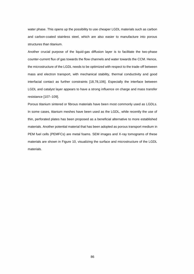
86
water phase. This opens up the possibility to use cheaper LGDL materials such as carbon
and carbon-coated stainless steel, which are also easier to manufacture into porous
structures than titanium.
Another crucial purpose of the liquid-gas diffusion layer is to facilitate the two-phase
counter-current flux of gas towards the flow channels and water towards the CCM. Hence,
the microstructure of the LGDL needs to be optimized with respect to the trade-off between
mass and electron transport, with mechanical stability, thermal conductivity and good
interfacial contact as further constraints [18,78,106]. Especially the interface between
LGDL and catalyst layer appears to have a strong influence on charge and mass transfer
resistance [107–109].
Porous titanium sintered or fibrous materials have been most commonly used as LGDLs.
In some cases, titanium meshes have been used as the LGDL, while recently the use of
thin, perforated plates has been proposed as a beneficial alternative to more established
materials. Another potential material that has been adopted as porous transport medium in
PEM fuel cells (PEMFCs) are metal foams. SEM images and X-ray tomograms of these
materials are shown in Figure 10, visualizing the surface and microstructure of the LGDL
materials.
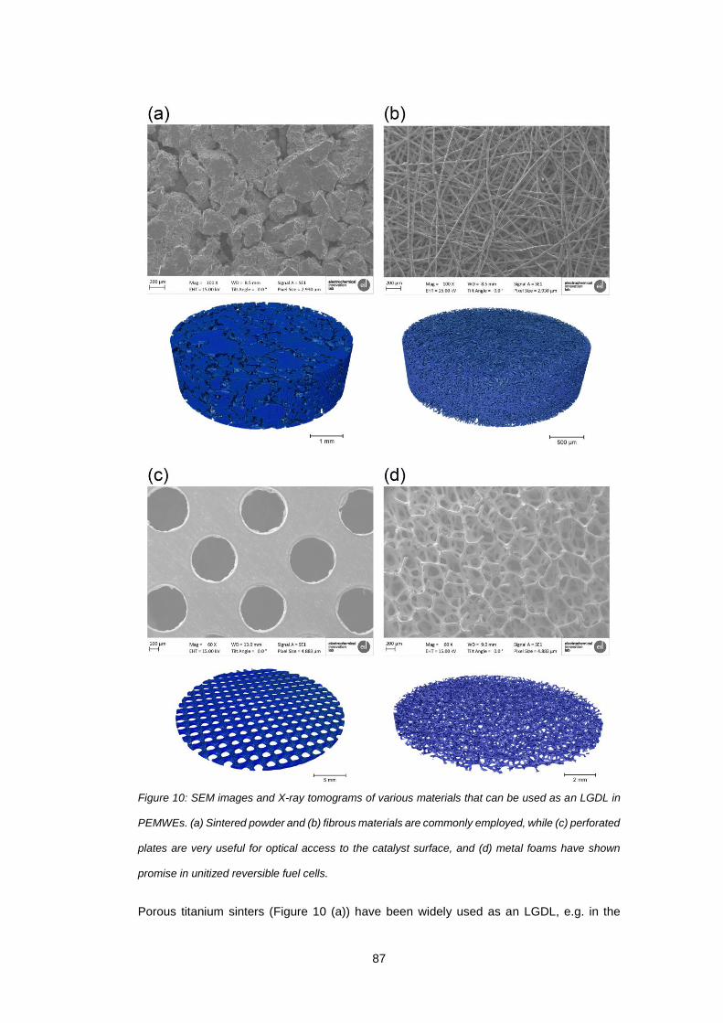
87
Figure 10: SEM images and X-ray tomograms of various materials that can be used as an LGDL in
PEMWEs. (a) Sintered powder and (b) fibrous materials are commonly employed, while (c) perforated
plates are very useful for optical access to the catalyst surface, and (d) metal foams have shown
promise in unitized reversible fuel cells.
Porous titanium sinters (Figure 10 (a)) have been widely used as an LGDL, e.g. in the
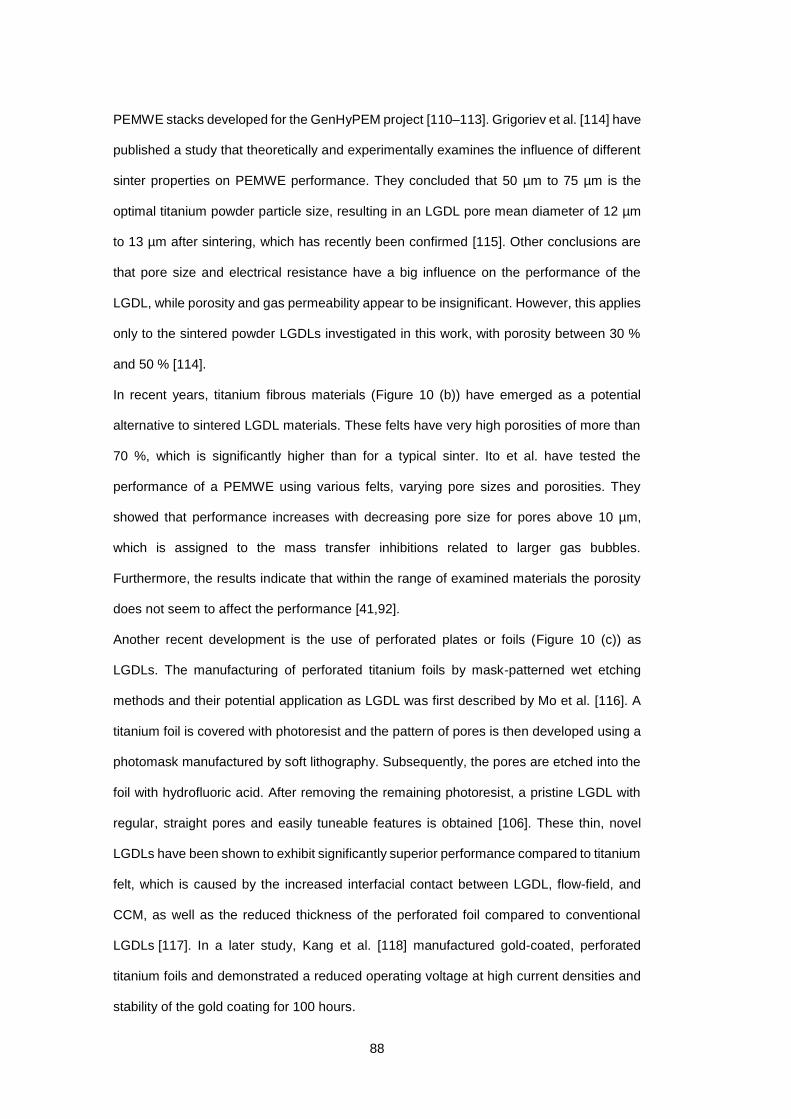
88
PEMWE stacks developed for the GenHyPEM project [110–113]. Grigoriev et al. [114] have
published a study that theoretically and experimentally examines the influence of different
sinter properties on PEMWE performance. They concluded that 50 µm to 75 µm is the
optimal titanium powder particle size, resulting in an LGDL pore mean diameter of 12 µm
to 13 µm after sintering, which has recently been confirmed [115]. Other conclusions are
that pore size and electrical resistance have a big influence on the performance of the
LGDL, while porosity and gas permeability appear to be insignificant. However, this applies
only to the sintered powder LGDLs investigated in this work, with porosity between 30 %
and 50 % [114].
In recent years, titanium fibrous materials (Figure 10 (b)) have emerged as a potential
alternative to sintered LGDL materials. These felts have very high porosities of more than
70 %, which is significantly higher than for a typical sinter. Ito et al. have tested the
performance of a PEMWE using various felts, varying pore sizes and porosities. They
showed that performance increases with decreasing pore size for pores above 10 µm,
which is assigned to the mass transfer inhibitions related to larger gas bubbles.
Furthermore, the results indicate that within the range of examined materials the porosity
does not seem to affect the performance [41,92].
Another recent development is the use of perforated plates or foils (Figure 10 (c)) as
LGDLs. The manufacturing of perforated titanium foils by mask-patterned wet etching
methods and their potential application as LGDL was first described by Mo et al. [116]. A
titanium foil is covered with photoresist and the pattern of pores is then developed using a
photomask manufactured by soft lithography. Subsequently, the pores are etched into the
foil with hydrofluoric acid. After removing the remaining photoresist, a pristine LGDL with
regular, straight pores and easily tuneable features is obtained [106]. These thin, novel
LGDLs have been shown to exhibit significantly superior performance compared to titanium
felt, which is caused by the increased interfacial contact between LGDL, flow-field, and
CCM, as well as the reduced thickness of the perforated foil compared to conventional
LGDLs [117]. In a later study, Kang et al. [118] manufactured gold-coated, perforated
titanium foils and demonstrated a reduced operating voltage at high current densities and
stability of the gold coating for 100 hours.
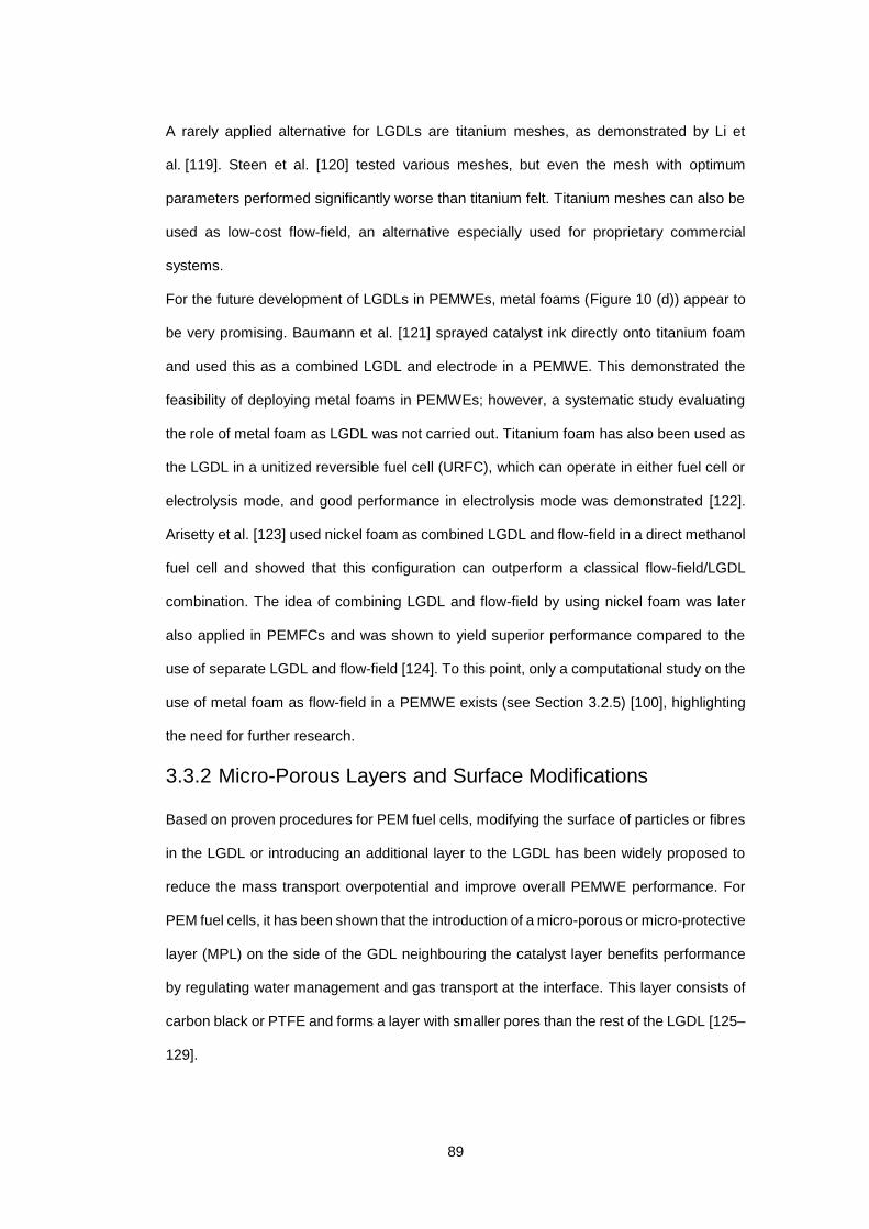
89
A rarely applied alternative for LGDLs are titanium meshes, as demonstrated by Li et
al. [119]. Steen et al. [120] tested various meshes, but even the mesh with optimum
parameters performed significantly worse than titanium felt. Titanium meshes can also be
used as low-cost flow-field, an alternative especially used for proprietary commercial
systems.
For the future development of LGDLs in PEMWEs, metal foams (Figure 10 (d)) appear to
be very promising. Baumann et al. [121] sprayed catalyst ink directly onto titanium foam
and used this as a combined LGDL and electrode in a PEMWE. This demonstrated the
feasibility of deploying metal foams in PEMWEs; however, a systematic study evaluating
the role of metal foam as LGDL was not carried out. Titanium foam has also been used as
the LGDL in a unitized reversible fuel cell (URFC), which can operate in either fuel cell or
electrolysis mode, and good performance in electrolysis mode was demonstrated [122].
Arisetty et al. [123] used nickel foam as combined LGDL and flow-field in a direct methanol
fuel cell and showed that this configuration can outperform a classical flow-field/LGDL
combination. The idea of combining LGDL and flow-field by using nickel foam was later
also applied in PEMFCs and was shown to yield superior performance compared to the
use of separate LGDL and flow-field [124]. To this point, only a computational study on the
use of metal foam as flow-field in a PEMWE exists (see Section 3.2.5) [100], highlighting
the need for further research.
3.3.2 Micro-Porous Layers and Surface Modifications
Based on proven procedures for PEM fuel cells, modifying the surface of particles or fibres
in the LGDL or introducing an additional layer to the LGDL has been widely proposed to
reduce the mass transport overpotential and improve overall PEMWE performance. For
PEM fuel cells, it has been shown that the introduction of a micro-porous or micro-protective
layer (MPL) on the side of the GDL neighbouring the catalyst layer benefits performance
by regulating water management and gas transport at the interface. This layer consists of
carbon black or PTFE and forms a layer with smaller pores than the rest of the LGDL [125–
129].
90
3.3.2.1 Micro-Porous Layers
Unfortunately, carbon or PTFE MPLs are not stable in the corrosive environment at the
LGDL/catalyst layer interface at the anode of a PEMWE, therefore, other materials have
been applied, trying to mimic the effect of the MPL in PEMFCs. Lettenmeier et al. [130]
created an MPL by coating a titanium sinter with porous titanium via thermal spraying and
demonstrated its superior performance, particularly at current densities exceeding
2 A cm-2. Sung et al. [131] used a coating of IrO2/Ta2O5 to produce a reactive MPL to
convert active oxygen species to oxygen, but did not compare the performance of their
system with a reference. Coating carbon paper with carbon black and subsequently with
IrO2 has been shown to yield an LGDL and MPL stable for 2000 hours, but no performance
comparison to a conventional PEMWE system was made [132]. Kang et al. [79] used micro
(~5 µm) and spherical nano (30 -50 nm) titanium particles to create an MPL on an LGDL
with small, straight, regular pores via low-temperature air spraying. It was found that micro-
particles yielded stronger performance improvement than nano-particles. A significant
performance improvement (1.707 V to 1.687 V at 2 A cm-2) was found for the micro MPL.
High-speed imaging showed that the MPL increased the number of pores providing active
catalyst sites. Schuler et al. [133] created sintered powder LGDL with MPLs of different
pore sizes and porosities; they showed a performance improvement and a reduction of up
to 60 mV with the use of an MPL compared to a conventional sintered powder LGDL.
The effect of coatings to provide an MPL has also been investigated in unitized reversible
fuel cells (URFCs). Ito et al. [134] used a layer of PTFE coating on titanium felt as the LGDL
in a URFC. They found that the influence of the modified LGDL depends on fibre size, but
a positive effect was only shown for fuel cell mode, not for electrolysis operation. Hwang et
al. confirmed many of these findings [135] and later created an MPL on titanium felt by
applying titanium powder and showed improved performance in a URFC for fuel cell
operation. No performance improvement was found in electrolysis mode; however, the
system was only tested up to 1 A cm-2 [136].
Building on the idea of an MPL, the use of LGDLs with graded porosity, increasing towards
the flow channels, has been shown to be beneficial in PEMFCs [137–139]. Lettenmeier et
al. [140] produced a sinter-like structure with a graded pore size via vacuum plasma
91
spraying. However, the authors could not show a significant performance improvement
using this novel material as the LGDL in a PEMWE. In a similar approach, Kang et al. [141]
created an LGDL structure with a gradual decrease in LGDL pore size. The authors
introduced the concept of an in-plane transport enhancement layer, combining two LGDLs
with straight, circular pores; one with large pores (~830 𝜇m) neighbouring the flow
channels, and a second one below it with significantly smaller pores (~100 𝜇m). Results
show a slight improvement in performance with the use of the enhancement layer. The
authors attribute this to an improvement in access to pores, which would have otherwise
been covered by the land areas of the flow plates.
3.3.2.2 Surface and Structural Modifications
For PEMFCs, chemical modification of the gas diffusion layer, e.g. by adding a hydrophobic
agent such as PTFE, has been demonstrated to be feasible, stable, and beneficial to
performance [142–145]. The chemical modification of the surface changes the contact
angle of gas and water, favouring the transport of one or the other in specific areas or
across the entire active area. The link between LGDL wettability (contact angle) and
PEMWE performance is well established [52,119,146].
However, little work has focused on varying the wettability of LGDLs for PEMWEs. Li et
al. [147] applied a hydrophobic monolayer of n-octadecyl tri-chlorosilane onto the surface
of a titanium LGDL. They could not demonstrate any performance improvement compared
to an untreated LGDL, but observed more frequent bubble detachment from the LGDL
surface. Bystron et al. [148] etched titanium felts in hydrochloric acid, creating a titanium
hydride sublayer. The authors showed significantly improved performance (voltage
reduction of around 0.15 V at 0.5 A cm-2) for more than 100 hours for felts treated in that
manner. Kang et al. [149] measured the PEMWE performance of PTFE-treated Toray
carbon paper and demonstrated a performance decrease with increasing hydrophobicity
(PTFE content).
Recent work by Suermann et al. [150] demonstrated the treatment of a fibrous titanium
LGDL with a femtosecond laser, inducing a high-surface structure, and showed a
performance improvement linked to the reduced contact resistance.
An alternative approach to improve mass transport through the LGDL is to introduce a
92
number of straight through-pores with significantly larger size than the natural pores of the
material. Lee et al. perforated a commercial sintered powder LGDL with 400 µm pores,
located in the channel regions of the PEMWE and in a distance of 2 mm from each other
along the channel length. The authors showed improved performance of the perforated
LGDL up to 9 A cm-2 and a reduction in the mass transport overpotential of up to 76.7 %,
which is attributed to the reduced gas saturation at the interface between catalyst layer and
LGDL.
3.3.3 Bubble Nucleation and Growth
Gas that is produced on the surface of the catalyst layer through electrochemical reaction
forms bubbles which are then transported through the LGDL and into the flow channels.
The nucleation of these bubbles is driven by the difference in chemical potential 𝜇 between
gas (𝑔) and liquid (𝑙) phase at the conditions found in the liquid phase at nucleation [151].
Δ𝜇 = 𝜇𝑙(𝑝𝑙 , 𝑇) − 𝜇𝑔(𝑝𝑙 , 𝑇) > 0 (Equation 3-12)
This driving force can be expressed in terms of temperature, pressure, the Boltzmann
constant 𝑘𝐵 and the pressure in the liquid phase 𝑝𝑙 [146,151]:
Δ𝜇 = 𝑘𝐵𝑇 ln𝑝𝑔
𝑝𝑙= 𝑘𝐵𝑇 ln 𝑆 , (Equation 3-13)
with the supersaturation S. The pressure in the gas phase 𝑝𝑔 is linked to the overall rate of
electrochemical gas production, which can be calculated using Faraday’s law (see Section
3.2.2).
The Gibbs free energy ∆𝐺 of a cluster of 𝑛 molecules is linked to this chemical potential
difference, the surface tension of a planar cluster 𝜎∞ and the surface area of the cluster
𝐴(𝑛) [151].
∆𝐺 = −𝑛∆𝜇 + 𝜎∞𝐴(𝑛) (Equation 3-14)
∆𝐺 has a maximum for the critical cluster size 𝑛𝑐. Clusters with less than 𝑛𝑐 molecules
require an increase in Gibbs free energy to grow and dissociate on average, while clusters
with more than 𝑛𝑐 molecules on average nucleate into bubbles [151].
𝑛𝑐 = [2
3
𝜎∞𝑠𝑙
𝑘𝐵𝑇 ln 𝑆]
3
(Equation 3-15)
The liquid phase factor is expressed as 𝑠𝑙 = (36𝜋)1 3⁄ 𝑣𝑙2 3⁄
, with the molecular volume of the
93
liquid phase 𝑣𝑙.
Increasing current density leads to a rise in gas production, which increases the
supersaturation; this reduces the critical cluster size and favours the formation of new gas
bubbles. However, the classical nucleation theory only describes bubble nucleation on a
regular surface under specific assumptions [151]. To our knowledge, there is no published
work on the nucleation of bubbles on the irregular surface of the catalyst layer under real-
world conditions.
Nouri-Khorasani et al. [146] developed a model of bubble nucleation and growth and its
effect on the electrolysis overpotential. They identified four phases from nucleation of a
bubble to its detachment from the LGDL surface. After sufficient supersaturation causes
nucleation, the bubble undergoes spherical growth within the walls of the surrounding pore
which is assumed to be a straight, vertical, cylindrical channel. Once the bubble diameter
is equal to the pore diameter, the bubble continues to grow cylindrically. Bubble detachment
occurs either due to the nucleation of a new bubble or as a result of changes in the balance
of drag, buoyancy, pressure, inertia and surface tension gradient forces. After detachment,
the bubble travels through the pore to the interface of LGDL and flow channel. It then
undergoes further spherical growth until it either coalesces with an adjacent bubble or
detaches from the LGDL surface due to the drag forces exerted by the convective flow of
water through the flow channel.
Li et al. [152] used optical high-speed imaging to observe the processes described
theoretically by Nouri-Khorasani. They used a novel, thin LGDL with straight, cylindrical
pores and observed spherical bubble growth along the wall of pores. This confirmed earlier
findings that bubble nucleation occurs only along the triple-phase boundary (see Section
3.4) [78,82]. Due to this limitation, and the relatively large pore diameter in this work (100
𝜇m), cylindrical growth and detachment from the LGDL surface were not observed. The
authors also found increasing bubble detachment diameters from the catalyst surface for
higher current density and temperature.
The detachment of bubbles from the LGDL surface has been visualized by neutron and X-
ray imaging. Hoeh et al. [83] found rapid, sudden detachment of bubbles followed by a slow
growth up to the critical size. The location of detachment and bubble growth was observed

94
to be constant, which implies the existence of preferential pathways through the LGDL.
Leonard et al. [84] demonstrated the same periodicity of growth and detachment and further
showed that detachment frequency and diameter increased with current density.
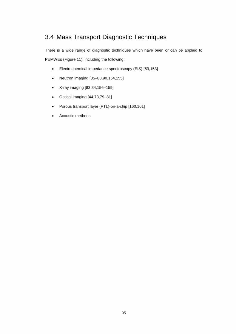
95
3.4 Mass Transport Diagnostic Techniques
There is a wide range of diagnostic techniques which have been or can be applied to
PEMWEs (Figure 11), including the following:
Electrochemical impedance spectroscopy (EIS) [59,153]
Neutron imaging [85–88,90,154,155]
X-ray imaging [83,84,156–159]
Optical imaging [44,73,79–81]
Porous transport layer (PTL)-on-a-chip [160,161]
Acoustic methods
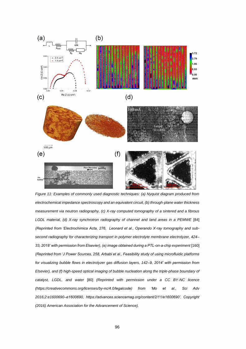
96
Figure 11: Examples of commonly used diagnostic techniques: (a) Nyquist diagram produced from
electrochemical impedance spectroscopy and an equivalent circuit, (b) through-plane water thickness
measurement via neutron radiography, (c) X-ray computed tomography of a sintered and a fibrous
LGDL material, (d) X-ray synchrotron radiography of channel and land areas in a PEMWE [84]
(Reprinted from ‘Electrochimica Acta, 276, Leonard et al., Operando X-ray tomography and sub-
second radiography for characterizing transport in polymer electrolyte membrane electrolyzer, 424–
33, 2018’ with permission from Elsevier), (e) image obtained during a PTL-on-a-chip experiment [160]
(Reprinted from ‘J Power Sources, 258, Arbabi et al., Feasibility study of using microfluidic platforms
for visualizing bubble flows in electrolyzer gas diffusion layers, 142–9, 2014’ with permission from
Elsevier), and (f) high-speed optical imaging of bubble nucleation along the triple-phase boundary of
catalyst, LGDL, and water [80] (Reprinted with permission under a CC BY-NC licence
(https://creativecommons.org/licenses/by-nc/4.0/legalcode) from ‘Mo et al., Sci Adv
2016;2:e1600690–e1600690, https://advances.sciencemag.org/content/2/11/e1600690’. Copyright
(2016) American Association for the Advancement of Science).
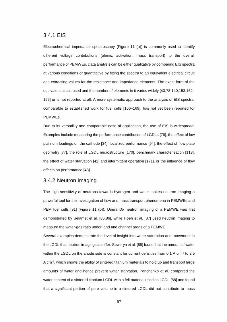
97
3.4.1 EIS
Electrochemical impedance spectroscopy (Figure 11 (a)) is commonly used to identify
different voltage contributions (ohmic, activation, mass transport) to the overall
performance of PEMWEs. Data analysis can be either qualitative by comparing EIS spectra
at various conditions or quantitative by fitting the spectra to an equivalent electrical circuit
and extracting values for the resistance and impedance elements. The exact form of the
equivalent circuit used and the number of elements in it varies widely [43,78,140,153,162–
165] or is not reported at all. A more systematic approach to the analysis of EIS spectra,
comparable to established work for fuel cells [166–169], has not yet been reported for
PEMWEs.
Due to its versatility and comparable ease of application, the use of EIS is widespread.
Examples include measuring the performance contribution of LGDLs [78], the effect of low
platinum loadings on the cathode [34], localized performance [94], the effect of flow plate
geometry [77], the role of LGDL microstructure [170], benchmark characterisation [113],
the effect of water starvation [42] and intermittent operation [171], or the influence of flow
effects on performance [43].
3.4.2 Neutron Imaging
The high sensitivity of neutrons towards hydrogen and water makes neutron imaging a
powerful tool for the investigation of flow and mass transport phenomena in PEMWEs and
PEM fuel cells [91] (Figure 11 (b)). Operando neutron imaging of a PEMWE was first
demonstrated by Selamet et al. [85,86], while Hoeh et al. [87] used neutron imaging to
measure the water-gas ratio under land and channel areas of a PEMWE.
Several examples demonstrate the level of insight into water saturation and movement in
the LGDL that neutron imaging can offer. Seweryn et al. [89] found that the amount of water
within the LGDL on the anode side is constant for current densities from 0.1 A cm-2 to 2.5
A cm-2, which shows the ability of sintered titanium materials to hold up and transport large
amounts of water and hence prevent water starvation. Panchenko et al. compared the
water content of a sintered titanium LGDL with a felt material used as LGDL [88] and found
that a significant portion of pore volume in a sintered LGDL did not contribute to mass
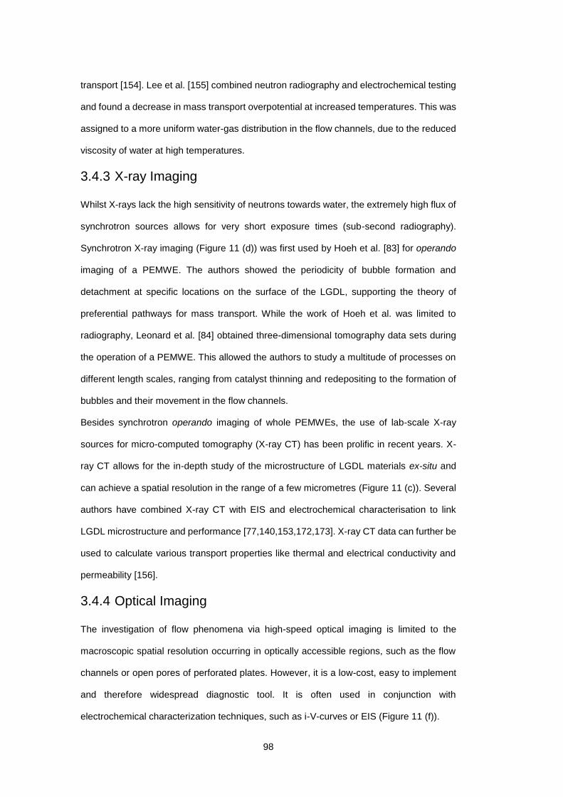
98
transport [154]. Lee et al. [155] combined neutron radiography and electrochemical testing
and found a decrease in mass transport overpotential at increased temperatures. This was
assigned to a more uniform water-gas distribution in the flow channels, due to the reduced
viscosity of water at high temperatures.
3.4.3 X-ray Imaging
Whilst X-rays lack the high sensitivity of neutrons towards water, the extremely high flux of
synchrotron sources allows for very short exposure times (sub-second radiography).
Synchrotron X-ray imaging (Figure 11 (d)) was first used by Hoeh et al. [83] for operando
imaging of a PEMWE. The authors showed the periodicity of bubble formation and
detachment at specific locations on the surface of the LGDL, supporting the theory of
preferential pathways for mass transport. While the work of Hoeh et al. was limited to
radiography, Leonard et al. [84] obtained three-dimensional tomography data sets during
the operation of a PEMWE. This allowed the authors to study a multitude of processes on
different length scales, ranging from catalyst thinning and redepositing to the formation of
bubbles and their movement in the flow channels.
Besides synchrotron operando imaging of whole PEMWEs, the use of lab-scale X-ray
sources for micro-computed tomography (X-ray CT) has been prolific in recent years. X-
ray CT allows for the in-depth study of the microstructure of LGDL materials ex-situ and
can achieve a spatial resolution in the range of a few micrometres (Figure 11 (c)). Several
authors have combined X-ray CT with EIS and electrochemical characterisation to link
LGDL microstructure and performance [77,140,153,172,173]. X-ray CT data can further be
used to calculate various transport properties like thermal and electrical conductivity and
permeability [156].
3.4.4 Optical Imaging
The investigation of flow phenomena via high-speed optical imaging is limited to the
macroscopic spatial resolution occurring in optically accessible regions, such as the flow
channels or open pores of perforated plates. However, it is a low-cost, easy to implement
and therefore widespread diagnostic tool. It is often used in conjunction with
electrochemical characterization techniques, such as i-V-curves or EIS (Figure 11 (f)).
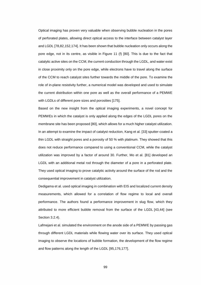
99
Optical imaging has proven very valuable when observing bubble nucleation in the pores
of perforated plates, allowing direct optical access to the interface between catalyst layer
and LGDL [78,82,152,174]. It has been shown that bubble nucleation only occurs along the
pore edge, not in its centre, as visible in Figure 11 (f) [80]. This is due to the fact that
catalytic active sites on the CCM, the current conduction through the LGDL, and water exist
in close proximity only on the pore edge, while electrons have to travel along the surface
of the CCM to reach catalyst sites further towards the middle of the pore. To examine the
role of in-plane resistivity further, a numerical model was developed and used to simulate
the current distribution within one pore as well as the overall performance of a PEMWE
with LGDLs of different pore sizes and porosities [175].
Based on the new insight from the optical imaging experiments, a novel concept for
PEMWEs in which the catalyst is only applied along the edges of the LGDL pores on the
membrane site has been proposed [80], which allows for a much higher catalyst utilization.
In an attempt to examine the impact of catalyst reduction, Kang et al. [33] sputter-coated a
thin LGDL with straight pores and a porosity of 50 % with platinum. They showed that this
does not reduce performance compared to using a conventional CCM, while the catalyst
utilization was improved by a factor of around 30. Further, Mo et al. [81] developed an
LGDL with an additional metal rod through the diameter of a pore in a perforated plate.
They used optical imaging to prove catalytic activity around the surface of the rod and the
consequential improvement in catalyst utilization.
Dedigama et al. used optical imaging in combination with EIS and localized current density
measurements, which allowed for a correlation of flow regime to local and overall
performance. The authors found a performance improvement in slug flow, which they
attributed to more efficient bubble removal from the surface of the LGDL [43,44] (see
Section 3.2.4).
Lafmejani et al. simulated the environment on the anode side of a PEMWE by passing gas
through different LGDL materials while flowing water over its surface. They used optical
imaging to observe the locations of bubble formation, the development of the flow regime
and flow patterns along the length of the LGDL [95,176,177].
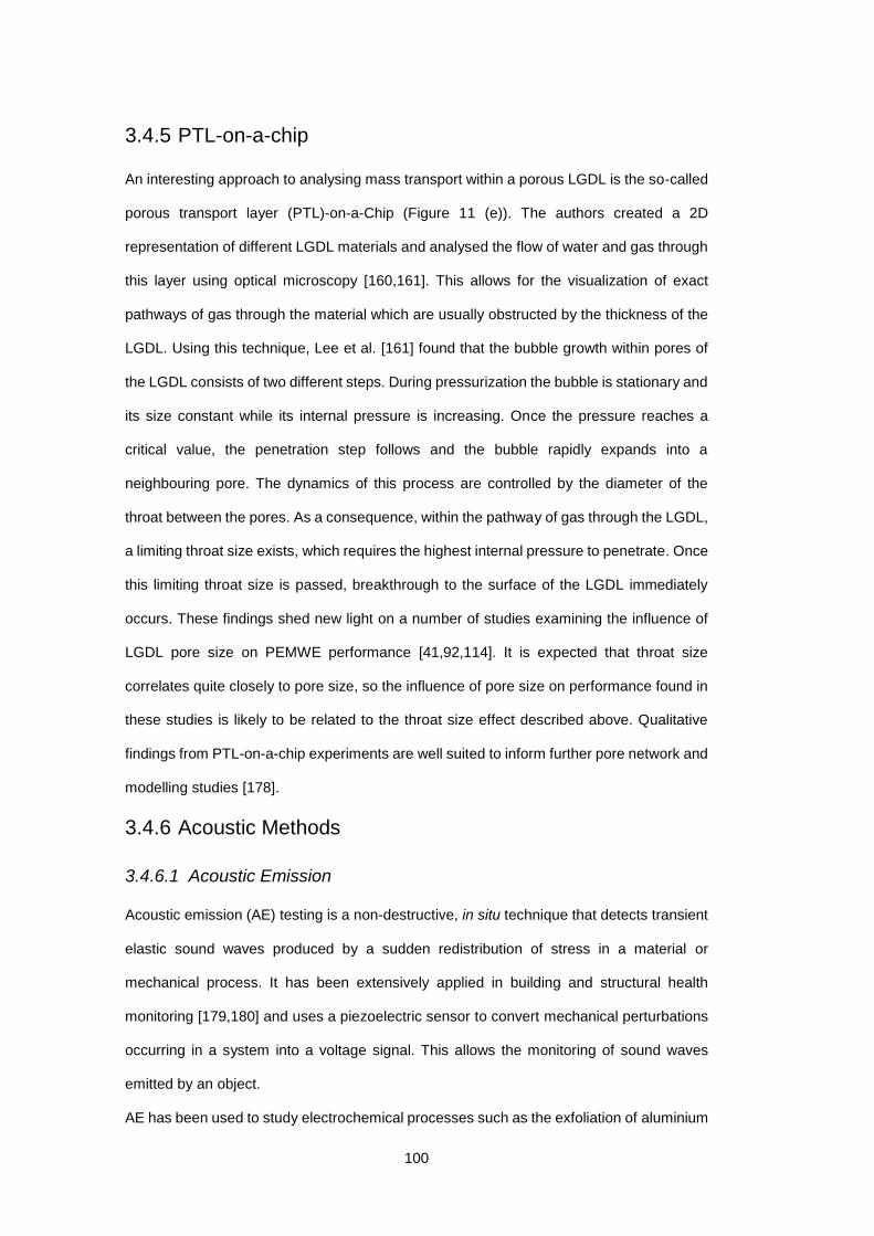
100
3.4.5 PTL-on-a-chip
An interesting approach to analysing mass transport within a porous LGDL is the so-called
porous transport layer (PTL)-on-a-Chip (Figure 11 (e)). The authors created a 2D
representation of different LGDL materials and analysed the flow of water and gas through
this layer using optical microscopy [160,161]. This allows for the visualization of exact
pathways of gas through the material which are usually obstructed by the thickness of the
LGDL. Using this technique, Lee et al. [161] found that the bubble growth within pores of
the LGDL consists of two different steps. During pressurization the bubble is stationary and
its size constant while its internal pressure is increasing. Once the pressure reaches a
critical value, the penetration step follows and the bubble rapidly expands into a
neighbouring pore. The dynamics of this process are controlled by the diameter of the
throat between the pores. As a consequence, within the pathway of gas through the LGDL,
a limiting throat size exists, which requires the highest internal pressure to penetrate. Once
this limiting throat size is passed, breakthrough to the surface of the LGDL immediately
occurs. These findings shed new light on a number of studies examining the influence of
LGDL pore size on PEMWE performance [41,92,114]. It is expected that throat size
correlates quite closely to pore size, so the influence of pore size on performance found in
these studies is likely to be related to the throat size effect described above. Qualitative
findings from PTL-on-a-chip experiments are well suited to inform further pore network and
modelling studies [178].
3.4.6 Acoustic Methods
3.4.6.1 Acoustic Emission
Acoustic emission (AE) testing is a non-destructive, in situ technique that detects transient
elastic sound waves produced by a sudden redistribution of stress in a material or
mechanical process. It has been extensively applied in building and structural health
monitoring [179,180] and uses a piezoelectric sensor to convert mechanical perturbations
occurring in a system into a voltage signal. This allows the monitoring of sound waves
emitted by an object.
AE has been used to study electrochemical processes such as the exfoliation of aluminium
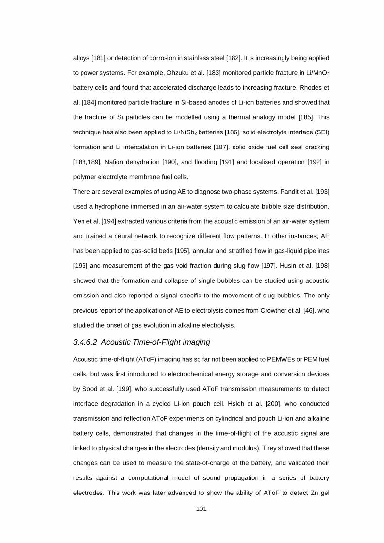
101
alloys [181] or detection of corrosion in stainless steel [182]. It is increasingly being applied
to power systems. For example, Ohzuku et al. [183] monitored particle fracture in Li/MnO2
battery cells and found that accelerated discharge leads to increasing fracture. Rhodes et
al. [184] monitored particle fracture in Si-based anodes of Li-ion batteries and showed that
the fracture of Si particles can be modelled using a thermal analogy model [185]. This
technique has also been applied to Li/NiSb2 batteries [186], solid electrolyte interface (SEI)
formation and Li intercalation in Li-ion batteries [187], solid oxide fuel cell seal cracking
[188,189], Nafion dehydration [190], and flooding [191] and localised operation [192] in
polymer electrolyte membrane fuel cells.
There are several examples of using AE to diagnose two-phase systems. Pandit et al. [193]
used a hydrophone immersed in an air-water system to calculate bubble size distribution.
Yen et al. [194] extracted various criteria from the acoustic emission of an air-water system
and trained a neural network to recognize different flow patterns. In other instances, AE
has been applied to gas-solid beds [195], annular and stratified flow in gas-liquid pipelines
[196] and measurement of the gas void fraction during slug flow [197]. Husin et al. [198]
showed that the formation and collapse of single bubbles can be studied using acoustic
emission and also reported a signal specific to the movement of slug bubbles. The only
previous report of the application of AE to electrolysis comes from Crowther et al. [46], who
studied the onset of gas evolution in alkaline electrolysis.
3.4.6.2 Acoustic Time-of-Flight Imaging
Acoustic time-of-flight (AToF) imaging has so far not been applied to PEMWEs or PEM fuel
cells, but was first introduced to electrochemical energy storage and conversion devices
by Sood et al. [199], who successfully used AToF transmission measurements to detect
interface degradation in a cycled Li-ion pouch cell. Hsieh et al. [200], who conducted
transmission and reflection AToF experiments on cylindrical and pouch Li-ion and alkaline
battery cells, demonstrated that changes in the time-of-flight of the acoustic signal are
linked to physical changes in the electrodes (density and modulus). They showed that these
changes can be used to measure the state-of-charge of the battery, and validated their
results against a computational model of sound propagation in a series of battery
electrodes. This work was later advanced to show the ability of AToF to detect Zn gel
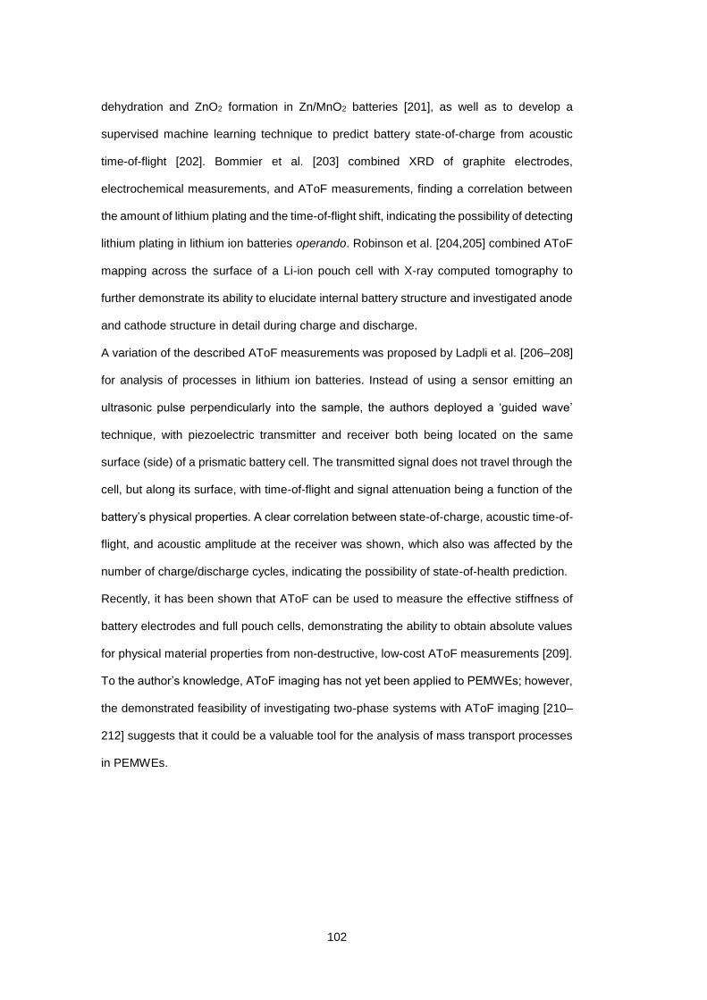
102
dehydration and ZnO2 formation in Zn/MnO2 batteries [201], as well as to develop a
supervised machine learning technique to predict battery state-of-charge from acoustic
time-of-flight [202]. Bommier et al. [203] combined XRD of graphite electrodes,
electrochemical measurements, and AToF measurements, finding a correlation between
the amount of lithium plating and the time-of-flight shift, indicating the possibility of detecting
lithium plating in lithium ion batteries operando. Robinson et al. [204,205] combined AToF
mapping across the surface of a Li-ion pouch cell with X-ray computed tomography to
further demonstrate its ability to elucidate internal battery structure and investigated anode
and cathode structure in detail during charge and discharge.
A variation of the described AToF measurements was proposed by Ladpli et al. [206–208]
for analysis of processes in lithium ion batteries. Instead of using a sensor emitting an
ultrasonic pulse perpendicularly into the sample, the authors deployed a ‘guided wave’
technique, with piezoelectric transmitter and receiver both being located on the same
surface (side) of a prismatic battery cell. The transmitted signal does not travel through the
cell, but along its surface, with time-of-flight and signal attenuation being a function of the
battery’s physical properties. A clear correlation between state-of-charge, acoustic time-of-
flight, and acoustic amplitude at the receiver was shown, which also was affected by the
number of charge/discharge cycles, indicating the possibility of state-of-health prediction.
Recently, it has been shown that AToF can be used to measure the effective stiffness of
battery electrodes and full pouch cells, demonstrating the ability to obtain absolute values
for physical material properties from non-destructive, low-cost AToF measurements [209].
To the author’s knowledge, AToF imaging has not yet been applied to PEMWEs; however,
the demonstrated feasibility of investigating two-phase systems with AToF imaging [210–
212] suggests that it could be a valuable tool for the analysis of mass transport processes
in PEMWEs.

103
4 Methodology

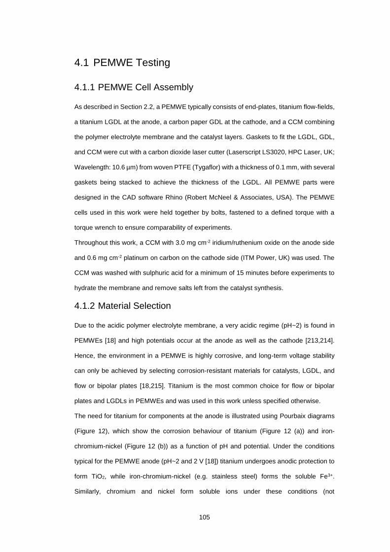
105
4.1 PEMWE Testing
4.1.1 PEMWE Cell Assembly
As described in Section 2.2, a PEMWE typically consists of end-plates, titanium flow-fields,
a titanium LGDL at the anode, a carbon paper GDL at the cathode, and a CCM combining
the polymer electrolyte membrane and the catalyst layers. Gaskets to fit the LGDL, GDL,
and CCM were cut with a carbon dioxide laser cutter (Laserscript LS3020, HPC Laser, UK;
Wavelength: 10.6 µm) from woven PTFE (Tygaflor) with a thickness of 0.1 mm, with several
gaskets being stacked to achieve the thickness of the LGDL. All PEMWE parts were
designed in the CAD software Rhino (Robert McNeel & Associates, USA). The PEMWE
cells used in this work were held together by bolts, fastened to a defined torque with a
torque wrench to ensure comparability of experiments.
Throughout this work, a CCM with 3.0 mg cm-2 iridium/ruthenium oxide on the anode side
and 0.6 mg cm-2 platinum on carbon on the cathode side (ITM Power, UK) was used. The
CCM was washed with sulphuric acid for a minimum of 15 minutes before experiments to
hydrate the membrane and remove salts left from the catalyst synthesis.
4.1.2 Material Selection
Due to the acidic polymer electrolyte membrane, a very acidic regime (pH~2) is found in
PEMWEs [18] and high potentials occur at the anode as well as the cathode [213,214].
Hence, the environment in a PEMWE is highly corrosive, and long-term voltage stability
can only be achieved by selecting corrosion-resistant materials for catalysts, LGDL, and
flow or bipolar plates [18,215]. Titanium is the most common choice for flow or bipolar
plates and LGDLs in PEMWEs and was used in this work unless specified otherwise.
The need for titanium for components at the anode is illustrated using Pourbaix diagrams
(Figure 12), which show the corrosion behaviour of titanium (Figure 12 (a)) and iron-
chromium-nickel (Figure 12 (b)) as a function of pH and potential. Under the conditions
typical for the PEMWE anode (pH~2 and 2 V [18]) titanium undergoes anodic protection to
form TiO2, while iron-chromium-nickel (e.g. stainless steel) forms the soluble Fe3+.
Similarly, chromium and nickel form soluble ions under these conditions (not
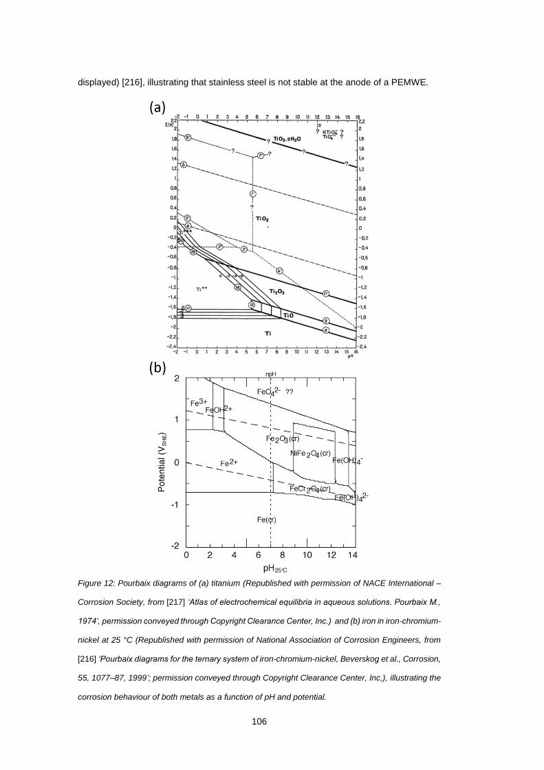
106
displayed) [216], illustrating that stainless steel is not stable at the anode of a PEMWE.
Figure 12: Pourbaix diagrams of (a) titanium (Republished with permission of NACE International –
Corrosion Society, from [217] ‘Atlas of electrochemical equilibria in aqueous solutions. Pourbaix M.,
1974’, permission conveyed through Copyright Clearance Center, Inc.) and (b) iron in iron-chromium-
nickel at 25 °C (Republished with permission of National Association of Corrosion Engineers, from
[216] ‘Pourbaix diagrams for the ternary system of iron-chromium-nickel, Beverskog et al., Corrosion,
55, 1077–87, 1999’; permission conveyed through Copyright Clearance Center, Inc,), illustrating the
corrosion behaviour of both metals as a function of pH and potential.
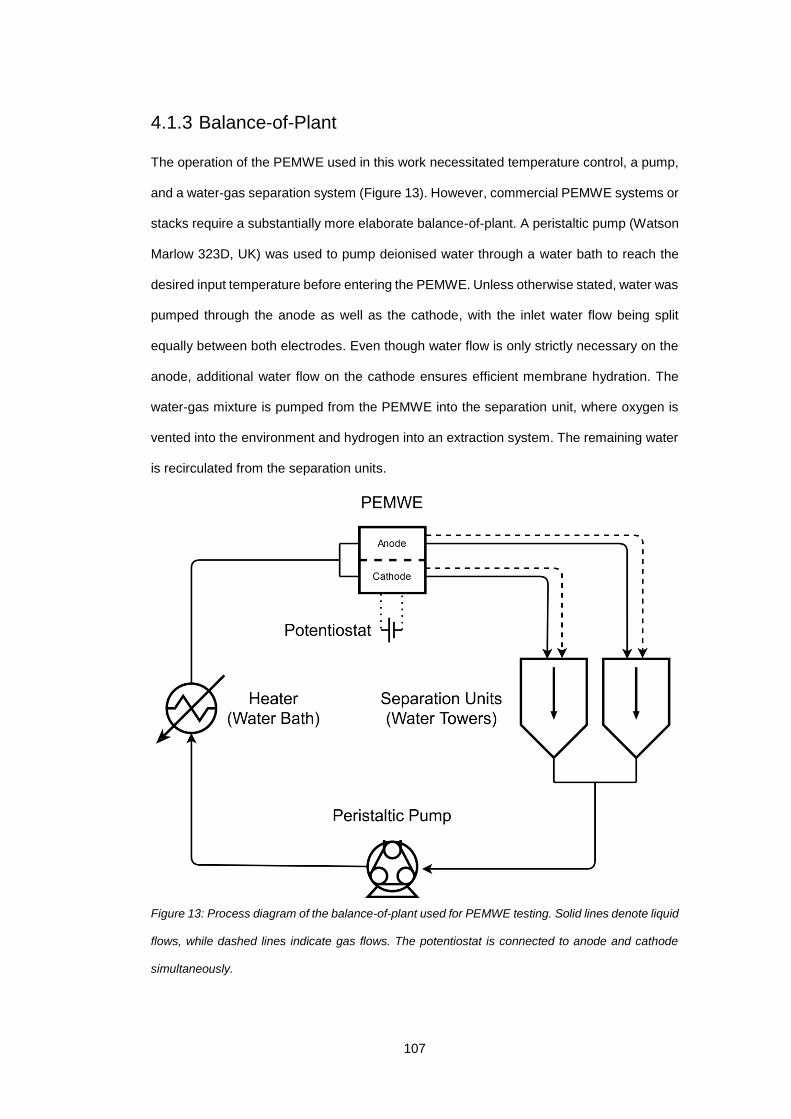
107
4.1.3 Balance-of-Plant
The operation of the PEMWE used in this work necessitated temperature control, a pump,
and a water-gas separation system (Figure 13). However, commercial PEMWE systems or
stacks require a substantially more elaborate balance-of-plant. A peristaltic pump (Watson
Marlow 323D, UK) was used to pump deionised water through a water bath to reach the
desired input temperature before entering the PEMWE. Unless otherwise stated, water was
pumped through the anode as well as the cathode, with the inlet water flow being split
equally between both electrodes. Even though water flow is only strictly necessary on the
anode, additional water flow on the cathode ensures efficient membrane hydration. The
water-gas mixture is pumped from the PEMWE into the separation unit, where oxygen is
vented into the environment and hydrogen into an extraction system. The remaining water
is recirculated from the separation units.
Figure 13: Process diagram of the balance-of-plant used for PEMWE testing. Solid lines denote liquid
flows, while dashed lines indicate gas flows. The potentiostat is connected to anode and cathode
simultaneously.
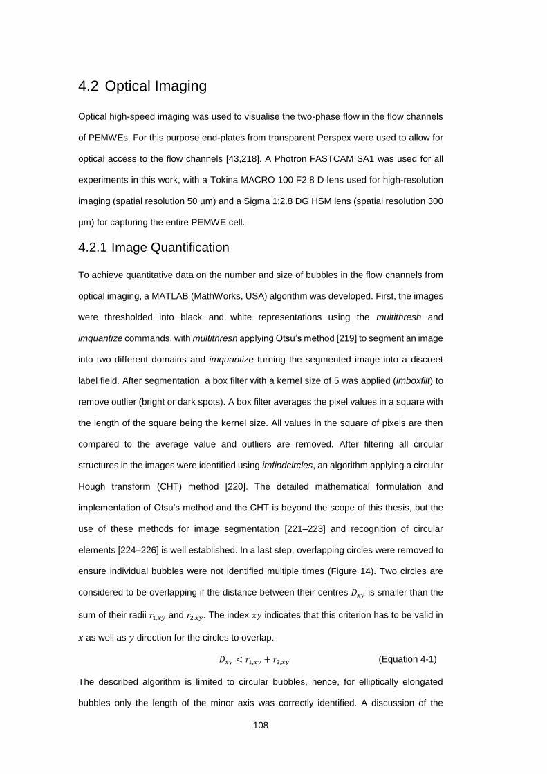
108
4.2 Optical Imaging
Optical high-speed imaging was used to visualise the two-phase flow in the flow channels
of PEMWEs. For this purpose end-plates from transparent Perspex were used to allow for
optical access to the flow channels [43,218]. A Photron FASTCAM SA1 was used for all
experiments in this work, with a Tokina MACRO 100 F2.8 D lens used for high-resolution
imaging (spatial resolution 50 µm) and a Sigma 1:2.8 DG HSM lens (spatial resolution 300
µm) for capturing the entire PEMWE cell.
4.2.1 Image Quantification
To achieve quantitative data on the number and size of bubbles in the flow channels from
optical imaging, a MATLAB (MathWorks, USA) algorithm was developed. First, the images
were thresholded into black and white representations using the multithresh and
imquantize commands, with multithresh applying Otsu’s method [219] to segment an image
into two different domains and imquantize turning the segmented image into a discreet
label field. After segmentation, a box filter with a kernel size of 5 was applied (imboxfilt) to
remove outlier (bright or dark spots). A box filter averages the pixel values in a square with
the length of the square being the kernel size. All values in the square of pixels are then
compared to the average value and outliers are removed. After filtering all circular
structures in the images were identified using imfindcircles, an algorithm applying a circular
Hough transform (CHT) method [220]. The detailed mathematical formulation and
implementation of Otsu’s method and the CHT is beyond the scope of this thesis, but the
use of these methods for image segmentation [221–223] and recognition of circular
elements [224–226] is well established. In a last step, overlapping circles were removed to
ensure individual bubbles were not identified multiple times (Figure 14). Two circles are
considered to be overlapping if the distance between their centres 𝐷𝑥𝑦 is smaller than the
sum of their radii 𝑟1,𝑥𝑦 and 𝑟2,𝑥𝑦. The index 𝑥𝑦 indicates that this criterion has to be valid in
𝑥 as well as 𝑦 direction for the circles to overlap.
𝐷𝑥𝑦 < 𝑟1,𝑥𝑦 + 𝑟2,𝑥𝑦 (Equation 4-1)
The described algorithm is limited to circular bubbles, hence, for elliptically elongated
bubbles only the length of the minor axis was correctly identified. A discussion of the
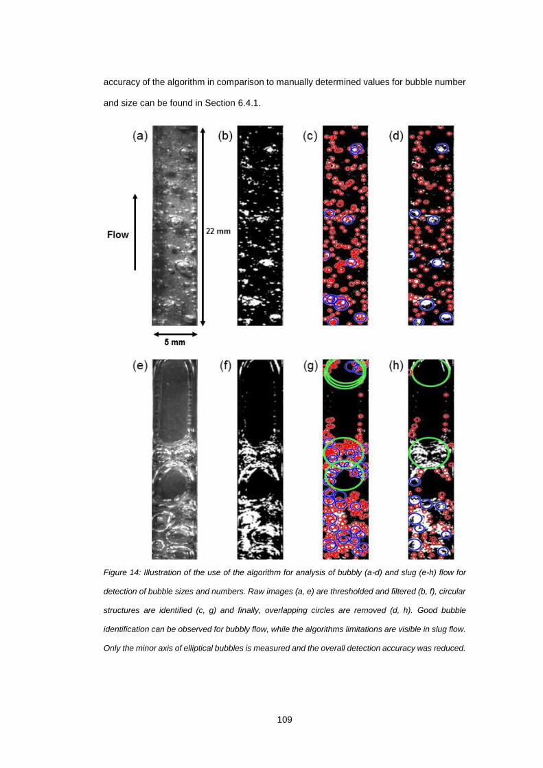
109
accuracy of the algorithm in comparison to manually determined values for bubble number
and size can be found in Section 6.4.1.
Figure 14: Illustration of the use of the algorithm for analysis of bubbly (a-d) and slug (e-h) flow for
detection of bubble sizes and numbers. Raw images (a, e) are thresholded and filtered (b, f), circular
structures are identified (c, g) and finally, overlapping circles are removed (d, h). Good bubble
identification can be observed for bubbly flow, while the algorithms limitations are visible in slug flow.
Only the minor axis of elliptical bubbles is measured and the overall detection accuracy was reduced.
110
4.3 Radiation-Based Imaging
Here, the scientific fundamentals of X-ray and neutron imaging, as well as the methodology
of image acquisition and analysis for both will be outlined, and the section will be finished
with a brief description of tomographic reconstruction, which is used to calculate three-
dimensional data sets from a series of two-dimensional projection images.
Certain image analysis steps, such as the extraction of porosity, tortuosity, and pore size
distribution from tomograms (Section 4.3.1.4), or the normalisation of radiographs with a
reference image (Section 4.3.2.4), will be presented exclusively in the context of either X-
ray or neutron imaging; however, this is to represent the techniques applied to specific data
sets in this work, while the underlying techniques are more general and can be applied to
any two- or three-dimensional image data.
4.3.1 X-ray Imaging
This section will introduce the production of X-ray radiation, its interaction with matter, and
how this is used for the design of X-ray imaging systems. Typical post-processing steps for
the reconstructed data sets are outlined, and the calculation of quantitative parameters
such as porosity, tortuosity or pore size distribution from 3D data sets explained. Lastly, a
lab-based system for the acquisition of X-ray computed tomograms (XCT) is presented.
4.3.1.1 Production of X-ray Radiation
X-ray photons originate either from the transition of an electron from an outer shell to a
vacancy on the inner shell caused by the ejection of a core electron, or from the
acceleration or deceleration of charged particles such as electrons [227]. The acceleration
of electrons in a magnetic field is commonly used for achieving high flux X-ray radiation in
synchrotrons, but will not be discussed further in this work.
The X-ray radiation in lab-based systems is produced by electrons being accelerated in a
high voltage electric field and fired at a target. The subsequent emission of X-ray photons
follows the two remaining mechanisms described above: discrete radiation at a number of
element-specific wavelengths due to high energy electrons filling core electron vacancies,
and a continuous radiation spectrum (Bremsstrahlung) caused by the deceleration of high-
111
speed electrons by either the nuclei electric field or direct collision with a nuclei [228]. The
resulting spectrum in an X-ray tube is a superposition of individual peaks and a continuous
distribution of photons as a function of energy. This distribution is asymmetrical with a tail
towards high energy photons and a maximum energy at the energy of the X-ray tube [227].
4.3.1.2 Interaction of X-ray Radiation with Matter
Upon interaction with a sample, X-ray photons are either transmitted, or absorbed via a
number of different mechanisms, most notably the photoelectric effect and elastic and
inelastic scattering. The production of an electron-positron pair and the emission of
radioactive radiation (photonuclear effect) are not relevant within the typical energy range
(between 5 keV and 150 keV) for X-ray spectroscopy [227]. The photoelectric effect, which
dominates the photon interactions in the relevant energy range [228], is caused by the
excitation of an electron by the incident X-ray photon. This electron is ejected, in turn
causing excitation of the atom which is relaxed when an electron from an outer shell falls
onto a lower energy level to fill the vacancy. Heavy atoms tend to emit the released energy
in the form of X-ray radiation, while in light elements the energy is released via electrons
(Auger effect) [227]. An overview of the interaction of X-ray radiation with a sample is shown
in Figure 15.
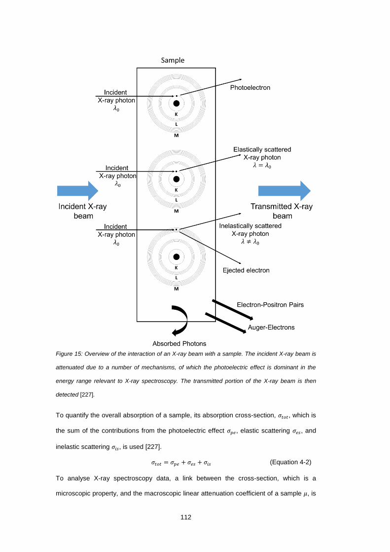
112
Figure 15: Overview of the interaction of an X-ray beam with a sample. The incident X-ray beam is
attenuated due to a number of mechanisms, of which the photoelectric effect is dominant in the
energy range relevant to X-ray spectroscopy. The transmitted portion of the X-ray beam is then
detected [227].
To quantify the overall absorption of a sample, its absorption cross-section, 𝜎𝑡𝑜𝑡, which is
the sum of the contributions from the photoelectric effect 𝜎𝑝𝑒, elastic scattering 𝜎𝑒𝑠, and
inelastic scattering 𝜎𝑖𝑠, is used [227].
𝜎𝑡𝑜𝑡 = 𝜎𝑝𝑒 + 𝜎𝑒𝑠 + 𝜎𝑖𝑠 (Equation 4-2)
To analyse X-ray spectroscopy data, a link between the cross-section, which is a
microscopic property, and the macroscopic linear attenuation coefficient of a sample 𝜇, is
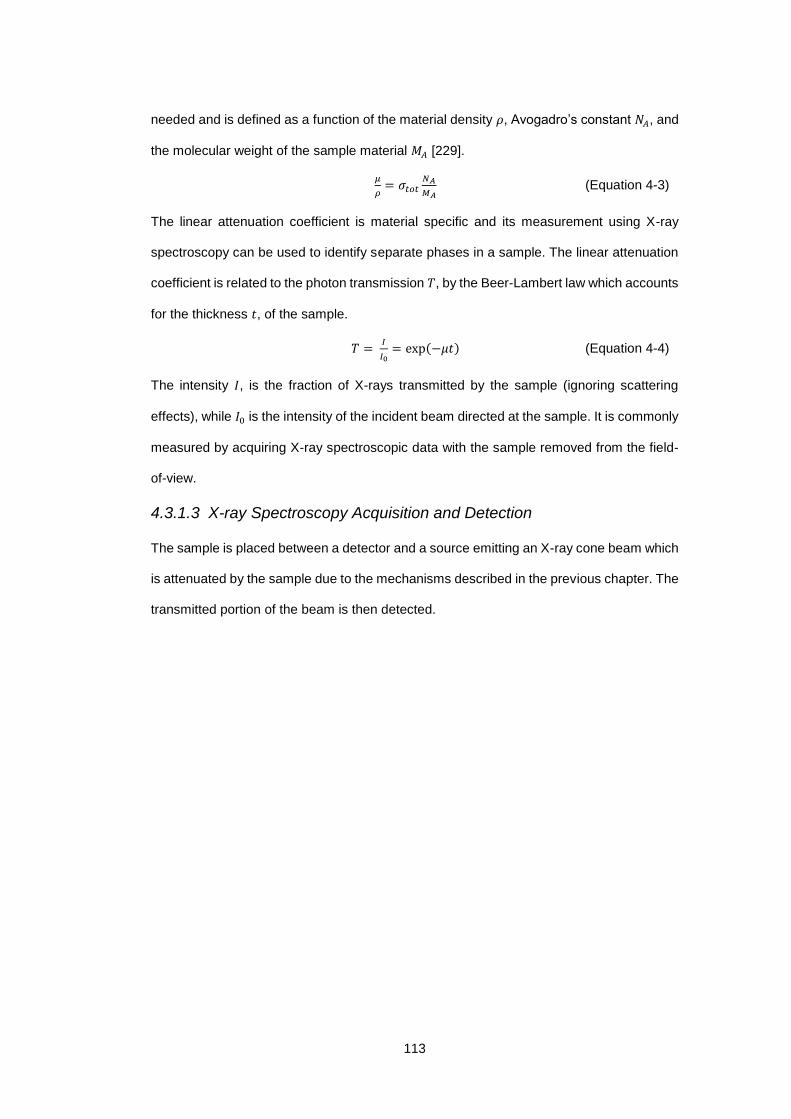
113
needed and is defined as a function of the material density 𝜌, Avogadro’s constant 𝑁𝐴, and
the molecular weight of the sample material 𝑀𝐴 [229].
𝜇
𝜌= 𝜎𝑡𝑜𝑡
𝑁𝐴
𝑀𝐴 (Equation 4-3)
The linear attenuation coefficient is material specific and its measurement using X-ray
spectroscopy can be used to identify separate phases in a sample. The linear attenuation
coefficient is related to the photon transmission 𝑇, by the Beer-Lambert law which accounts
for the thickness 𝑡, of the sample.
𝑇 = 𝐼
𝐼0= exp(−𝜇𝑡) (Equation 4-4)
The intensity 𝐼, is the fraction of X-rays transmitted by the sample (ignoring scattering
effects), while 𝐼0 is the intensity of the incident beam directed at the sample. It is commonly
measured by acquiring X-ray spectroscopic data with the sample removed from the field-
of-view.
4.3.1.3 X-ray Spectroscopy Acquisition and Detection
The sample is placed between a detector and a source emitting an X-ray cone beam which
is attenuated by the sample due to the mechanisms described in the previous chapter. The
transmitted portion of the beam is then detected.
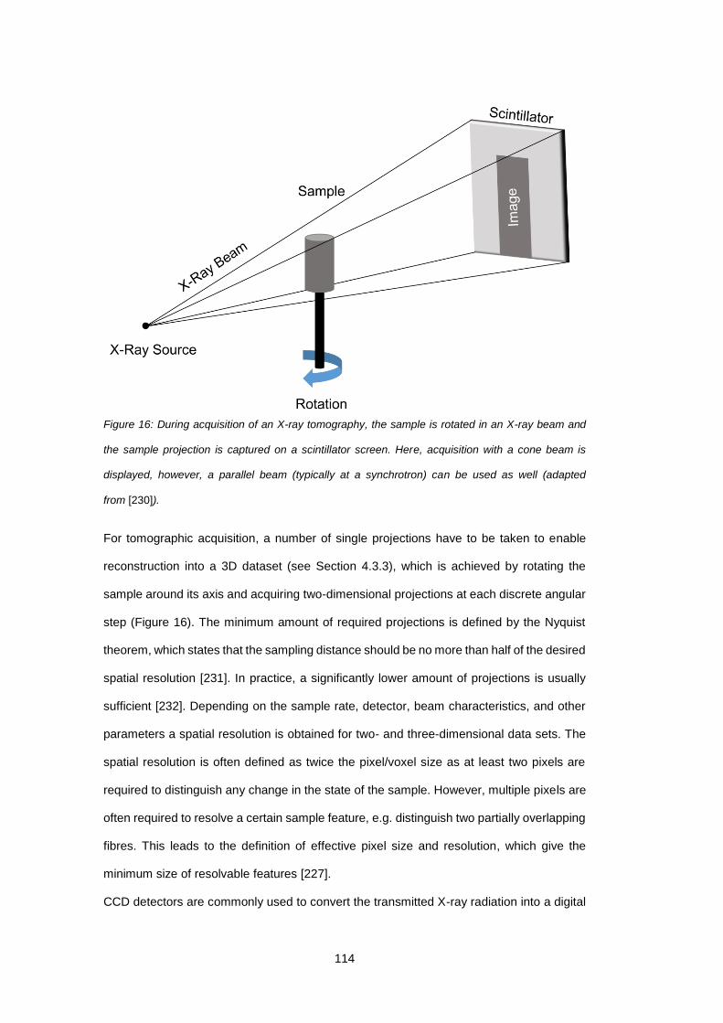
114
Figure 16: During acquisition of an X-ray tomography, the sample is rotated in an X-ray beam and
the sample projection is captured on a scintillator screen. Here, acquisition with a cone beam is
displayed, however, a parallel beam (typically at a synchrotron) can be used as well (adapted
from [230]).
For tomographic acquisition, a number of single projections have to be taken to enable
reconstruction into a 3D dataset (see Section 4.3.3), which is achieved by rotating the
sample around its axis and acquiring two-dimensional projections at each discrete angular
step (Figure 16). The minimum amount of required projections is defined by the Nyquist
theorem, which states that the sampling distance should be no more than half of the desired
spatial resolution [231]. In practice, a significantly lower amount of projections is usually
sufficient [232]. Depending on the sample rate, detector, beam characteristics, and other
parameters a spatial resolution is obtained for two- and three-dimensional data sets. The
spatial resolution is often defined as twice the pixel/voxel size as at least two pixels are
required to distinguish any change in the state of the sample. However, multiple pixels are
often required to resolve a certain sample feature, e.g. distinguish two partially overlapping
fibres. This leads to the definition of effective pixel size and resolution, which give the
minimum size of resolvable features [227].
CCD detectors are commonly used to convert the transmitted X-ray radiation into a digital
115
image. In a first step, a scintillator based on phosphor or a semiconductor converts the X-
ray radiation into light. The light is magnified if required and coupled via lenses or fibre
optics. In the last step, the optical signal is converted into an electrical one [233].
4.3.1.4 Image Quantification
To enable quantitative analysis and a more detailed comparison of different samples, key
metrics like porosity, tortuosity, and pore size distribution (PSD) can be extracted from the
reconstructed tomograms. In the first step, the data is segmented into different phases
based on greyscale values. As different materials have different attenuation coefficients,
the respective regions in the tomogram exhibit varying greyscale values. Hence, local
minima in the histogram mark phase transitions that can serve as the basis for manual
thresholding. In this case, all voxels to the left of the minimum are assigned to one phase
(e.g. phase 0), while the voxels to the right are assigned to a second phase (e.g. phase 1),
with errors and artefacts, such as beam hardening, ring artefacts, or partial volume effects,
potentially introducing uncertainty to the location of the phase transition in the histogram.
In many cases, this can be circumvented by applying filters before segmentation, or using
machine-learning segmentation algorithms [232]. However, these methods are beyond the
scope of this thesis. The product of image segmentation is a label field, assigning a phase-
specific value to each voxel. Unless stated otherwise, all image quantification was
performed in the software Avizo (Thermo Fisher Scientific, USA).
4.3.1.4.1 Porosity and Tortuosity
After segmentation, the porosity (or phase fraction) in a sample is easily determined from
the contribution of a specific phase to the overall area in a slice through the label field.
Typically, the fraction of a phase is averaged across all orthoslices to obtain the respective
volume fraction. For example, the tomogram of an LGDL is segmented into two distinct
phases: pores and solid phase/titanium. To determine the porosity of the LGDL, the fraction
of pore of the overall area is determined for every orthoslice and averaged across all slices.
Tortuosity was determined from XCT data using TauFactor [234], a Matlab application
which compares the diffusive transport in a porous media with and without convolutions of
the flow path.
116
4.3.1.4.2 Pore Network Model and PSD
Avizo provides a number of proprietary functions to extract the PSD from segmented XCT
data. The Separate Objects method is applied to the pore phase, creating a label field of
individually labelled pores. This label field is used as input for the Generate Pore Network
Model module, which transforms the separated pores into a pore network model (PNM)
consisting of a number of pores (spheres) connected by throats (cylinders). When
generating the PNM, Avizo also calculates the permeability and tortuosity of the sample,
as well as the flow rate of fluid per second through each throat. Applying a Distribution
Analysis module to the pore network model produces the PSD. To limit the analysis to
connected pores, hence excluding all pores without connection to the main pore network,
an Axis Connectivity module may be applied to the segmented data [235].
4.3.1.5 X-ray micro-computed Tomography using the Zeiss Xradia Versa
The Zeiss Xradia Versa XRM-520T (Figure 17) is a lab-based X-ray micro-tomography
system with a two-stage magnification design, capable of achieving a maximum spatial
resolution of 0.7 µm. As shown in Section 5.4.1, the smalles pore sizes in LGDL materials
are typically around 10 µm, making X-ray micro-tomography with the Zeiss Xradia Versa a
suitable tool. Radiation is produced from a tungsten target (NT100, Nordson DAGE) and
an X-ray tube operating in the voltage range from 30 kV to 160 kV and with a maximum
power of 10 W. A range of filters are available to avoid beam hardening effects, which occur
when using a polychromatic beam, as low energy X-ray photons are attenuated more
strongly due to the photoelectric effect [227,232]. Beam hardening causes artificial
variations in pixel intensity, typically a decreasing intensity profile from the edge to the
centre of the sample. Images are acquired using a scintillator coupled with an optical
magnification turret (0.4X, 4X, 20X, 40X) and a 2048×2048 pixels CCD detector. A scouting
video camera is used to align the sample to the detector and source during setup [232,236].
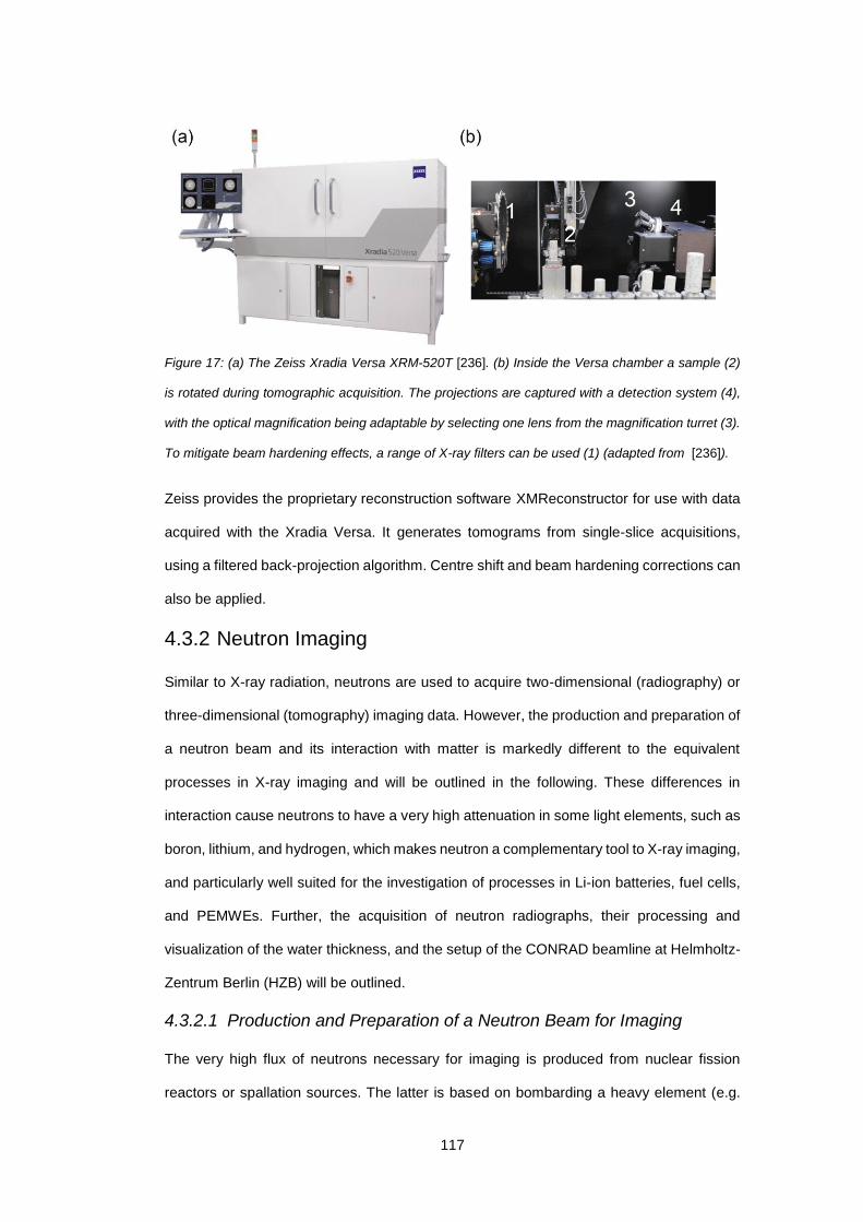
117
Figure 17: (a) The Zeiss Xradia Versa XRM-520T [236]. (b) Inside the Versa chamber a sample (2)
is rotated during tomographic acquisition. The projections are captured with a detection system (4),
with the optical magnification being adaptable by selecting one lens from the magnification turret (3).
To mitigate beam hardening effects, a range of X-ray filters can be used (1) (adapted from [236]).
Zeiss provides the proprietary reconstruction software XMReconstructor for use with data
acquired with the Xradia Versa. It generates tomograms from single-slice acquisitions,
using a filtered back-projection algorithm. Centre shift and beam hardening corrections can
also be applied.
4.3.2 Neutron Imaging
Similar to X-ray radiation, neutrons are used to acquire two-dimensional (radiography) or
three-dimensional (tomography) imaging data. However, the production and preparation of
a neutron beam and its interaction with matter is markedly different to the equivalent
processes in X-ray imaging and will be outlined in the following. These differences in
interaction cause neutrons to have a very high attenuation in some light elements, such as
boron, lithium, and hydrogen, which makes neutron a complementary tool to X-ray imaging,
and particularly well suited for the investigation of processes in Li-ion batteries, fuel cells,
and PEMWEs. Further, the acquisition of neutron radiographs, their processing and
visualization of the water thickness, and the setup of the CONRAD beamline at Helmholtz-
Zentrum Berlin (HZB) will be outlined.
4.3.2.1 Production and Preparation of a Neutron Beam for Imaging
The very high flux of neutrons necessary for imaging is produced from nuclear fission
reactors or spallation sources. The latter is based on bombarding a heavy element (e.g.
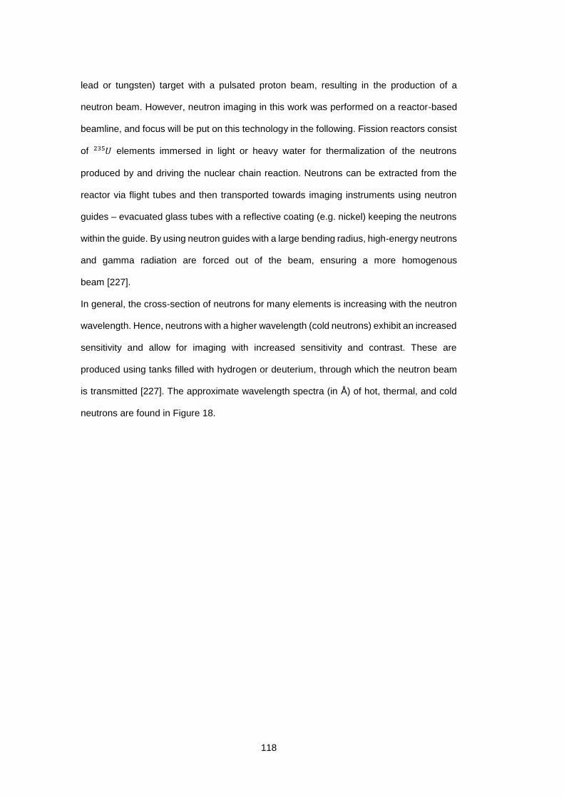
118
lead or tungsten) target with a pulsated proton beam, resulting in the production of a
neutron beam. However, neutron imaging in this work was performed on a reactor-based
beamline, and focus will be put on this technology in the following. Fission reactors consist
of 𝑈 235 elements immersed in light or heavy water for thermalization of the neutrons
produced by and driving the nuclear chain reaction. Neutrons can be extracted from the
reactor via flight tubes and then transported towards imaging instruments using neutron
guides – evacuated glass tubes with a reflective coating (e.g. nickel) keeping the neutrons
within the guide. By using neutron guides with a large bending radius, high-energy neutrons
and gamma radiation are forced out of the beam, ensuring a more homogenous
beam [227].
In general, the cross-section of neutrons for many elements is increasing with the neutron
wavelength. Hence, neutrons with a higher wavelength (cold neutrons) exhibit an increased
sensitivity and allow for imaging with increased sensitivity and contrast. These are
produced using tanks filled with hydrogen or deuterium, through which the neutron beam
is transmitted [227]. The approximate wavelength spectra (in Å) of hot, thermal, and cold
neutrons are found in Figure 18.
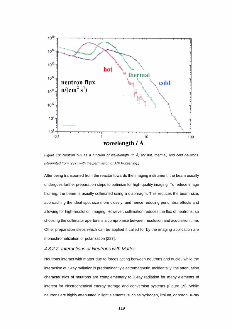
119
Figure 18: Neutron flux as a function of wavelength (in Å) for hot, thermal, and cold neutrons.
(Reprinted from [237], with the permission of AIP Publishing.)
After being transported from the reactor towards the imaging instrument, the beam usually
undergoes further preparation steps to optimize for high-quality imaging. To reduce image
blurring, the beam is usually collimated using a diaphragm. This reduces the beam size,
approaching the ideal spot size more closely, and hence reducing penumbra effects and
allowing for high-resolution imaging. However, collimation reduces the flux of neutrons, so
choosing the collimator aperture is a compromise between resolution and acquisition time.
Other preparation steps which can be applied if called for by the imaging application are
monochromatization or polarization [227].
4.3.2.2 Interactions of Neutrons with Matter
Neutrons interact with matter due to forces acting between neutrons and nuclei, while the
interaction of X-ray radiation is predominantly electromagnetic. Incidentally, the attenuation
characteristics of neutrons are complementary to X-ray radiation for many elements of
interest for electrochemical energy storage and conversion systems (Figure 19). While
neutrons are highly attenuated in light elements, such as hydrogen, lithium, or boron, X-ray

120
radiation is subject to a regular increase of attenuation with atomic number [227]. This
makes neutron imaging a powerful tool for visualization and quantification of processes in
electrochemical energy storage and conversion devices, such as PEMWEs [88,90], PEM
fuel cells [238,239], and lithium-ion batteries [240]. Further, neutrons interact with the
magnetic moment of nuclei, allowing for visualization of magnetic fields and domains [91].
However, this is beyond the scope of this thesis.
The main mechanisms of neutron attenuation are absorption and scattering. Absorption
occurs when a neutron is captured by a nucleus, leading to nuclear decay and the
consequent emission of fission products, such as α-particles, neutrons, or γ-radiation.
Scattering of neutrons is caused by the interaction of the neutron with the potential force of
a nucleus, which depends on the nucleus configuration in a complex manner and is not a
continuous function of nucleus size [227].
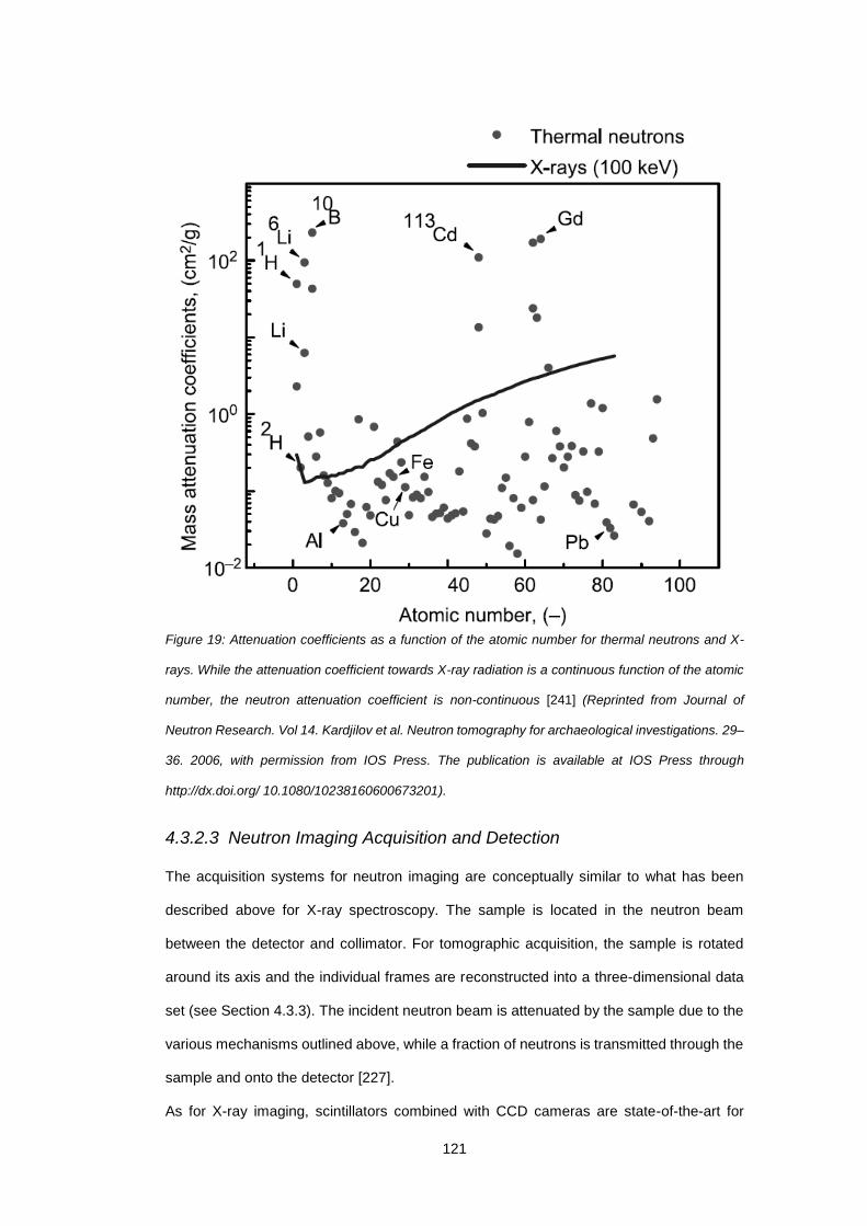
121
Figure 19: Attenuation coefficients as a function of the atomic number for thermal neutrons and X-
rays. While the attenuation coefficient towards X-ray radiation is a continuous function of the atomic
number, the neutron attenuation coefficient is non-continuous [241] (Reprinted from Journal of
Neutron Research. Vol 14. Kardjilov et al. Neutron tomography for archaeological investigations. 29–
36. 2006, with permission from IOS Press. The publication is available at IOS Press through
http://dx.doi.org/ 10.1080/10238160600673201).
4.3.2.3 Neutron Imaging Acquisition and Detection
The acquisition systems for neutron imaging are conceptually similar to what has been
described above for X-ray spectroscopy. The sample is located in the neutron beam
between the detector and collimator. For tomographic acquisition, the sample is rotated
around its axis and the individual frames are reconstructed into a three-dimensional data
set (see Section 4.3.3). The incident neutron beam is attenuated by the sample due to the
various mechanisms outlined above, while a fraction of neutrons is transmitted through the
sample and onto the detector [227].
As for X-ray imaging, scintillators combined with CCD cameras are state-of-the-art for
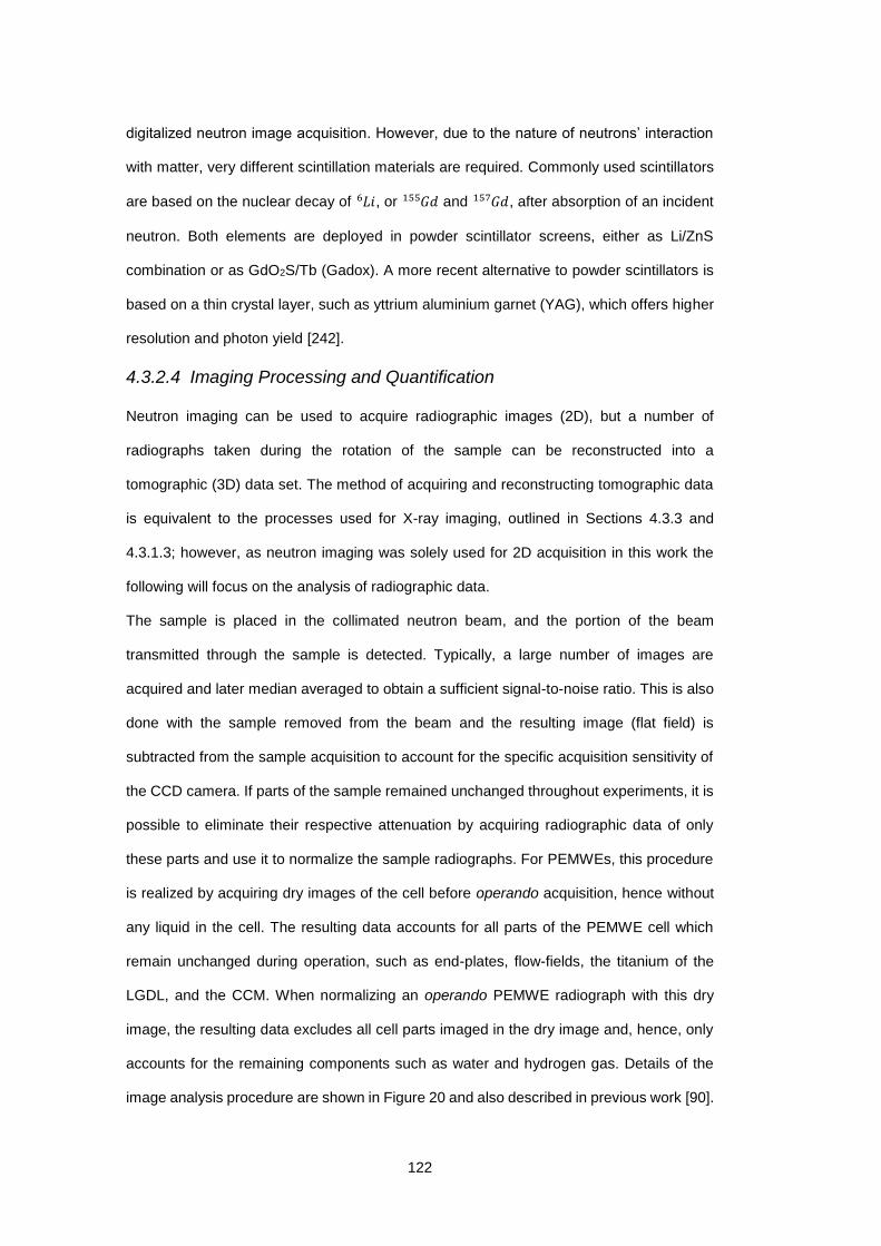
122
digitalized neutron image acquisition. However, due to the nature of neutrons’ interaction
with matter, very different scintillation materials are required. Commonly used scintillators
are based on the nuclear decay of 𝐿𝑖 6 , or 𝐺𝑑
155 and 𝐺𝑑 157 , after absorption of an incident
neutron. Both elements are deployed in powder scintillator screens, either as Li/ZnS
combination or as GdO2S/Tb (Gadox). A more recent alternative to powder scintillators is
based on a thin crystal layer, such as yttrium aluminium garnet (YAG), which offers higher
resolution and photon yield [242].
4.3.2.4 Imaging Processing and Quantification
Neutron imaging can be used to acquire radiographic images (2D), but a number of
radiographs taken during the rotation of the sample can be reconstructed into a
tomographic (3D) data set. The method of acquiring and reconstructing tomographic data
is equivalent to the processes used for X-ray imaging, outlined in Sections 4.3.3 and
4.3.1.3; however, as neutron imaging was solely used for 2D acquisition in this work the
following will focus on the analysis of radiographic data.
The sample is placed in the collimated neutron beam, and the portion of the beam
transmitted through the sample is detected. Typically, a large number of images are
acquired and later median averaged to obtain a sufficient signal-to-noise ratio. This is also
done with the sample removed from the beam and the resulting image (flat field) is
subtracted from the sample acquisition to account for the specific acquisition sensitivity of
the CCD camera. If parts of the sample remained unchanged throughout experiments, it is
possible to eliminate their respective attenuation by acquiring radiographic data of only
these parts and use it to normalize the sample radiographs. For PEMWEs, this procedure
is realized by acquiring dry images of the cell before operando acquisition, hence without
any liquid in the cell. The resulting data accounts for all parts of the PEMWE cell which
remain unchanged during operation, such as end-plates, flow-fields, the titanium of the
LGDL, and the CCM. When normalizing an operando PEMWE radiograph with this dry
image, the resulting data excludes all cell parts imaged in the dry image and, hence, only
accounts for the remaining components such as water and hydrogen gas. Details of the
image analysis procedure are shown in Figure 20 and also described in previous work [90].

123
Figure 20: (a) The PEMWE is placed in a neutron beam. Due to the material-dependent attenuation
of the neutrons, a radiographic image of the PEMWE is captured by the detector. (b) Each set of
images is first filtered to remove outliers and averaged using a median. Then, the averaged dark-field
is subtracted from the resulting image. This is then normalized with a dry image (also averaged) to
obtain the final image. The greyscale values can be converted into the water thickness using the
Beer-Lambert law. (c) The water thickness in the rib (land) areas is analysed separately by applying
a mask, discarding the water thickness in the flow channels.
124
The attenuation of neutrons follows the Beer-Lambert law [227], so if image analysis yields
radiographic data that only accounts for one component (e.g. water) the thickness of that
component in the through-plane imaging direction can be calculated. This requires
knowledge of the linear attenuation coefficient 𝜇 for the component, which is a function of
the sample thickness and the distance between sample and detector. The Beer-Lambert
law has been described in Section 4.3.1.2, and examples of its application to neutron
imaging can be found in literature [85,88,90].
4.3.2.5 CONRAD Neutron Beamline
Neutron imaging results presented in this work were acquired at the CONRAD beamline at
Helmholtz-Zentrum Berlin (HZB) [243,244], shown in Figure 21. CONRAD uses a beam of
cold neutrons with a flux of 2.4 × 10⁷ n cm−2s−1 and a CCD detector camera (Andor, 2048
× 2048 pixels) [243]. A spatial resolution of 20 µm at a field-of-view of 13 mm × 13 mm can
be achieved [243], with rotational and translational stages allowing for sample positioning
and tomographic acquisition. As outlined in Section 5.4.2, neutron imaging was used to
visualize the entire PEMWE active area, with flow-field features being in the millimetre
range, making neutron radiography at the CONRAD neutron beamline a suitable tool. A
transparent crystal scintillator is used for neutron detection [242].
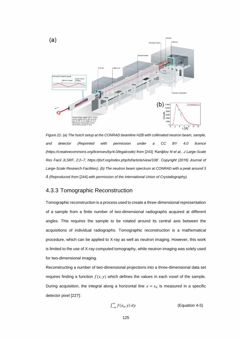
125
Figure 21: (a) The hutch setup at the CONRAD beamline HZB with collimated neutron beam, sample,
and detector (Reprinted with permission under a CC BY 4.0 licence
(https://creativecommons.org/licenses/by/4.0/legalcode) from [243] ‘Kardjilov N et al., J Large-Scale
Res Facil JLSRF, 2:2–7, https://jlsrf.org/index.php/lsf/article/view/108’. Copyright (2016) Journal of
Large-Scale Research Facilities). (b) The neutron beam spectrum at CONRAD with a peak around 3
Å (Reproduced from [244] with permission of the International Union of Crystallography).
4.3.3 Tomographic Reconstruction
Tomographic reconstruction is a process used to create a three-dimensional representation
of a sample from a finite number of two-dimensional radiographs acquired at different
angles. This requires the sample to be rotated around its central axis between the
acquisitions of individual radiographs. Tomographic reconstruction is a mathematical
procedure, which can be applied to X-ray as well as neutron imaging. However, this work
is limited to the use of X-ray computed tomography, while neutron imaging was solely used
for two-dimensional imaging.
Reconstructing a number of two-dimensional projections into a three-dimensional data set
requires finding a function 𝑓(𝑥, 𝑦) which defines the values in each voxel of the sample.
During acquisition, the integral along a horizontal line 𝑥 = 𝑥0 is measured in a specific
detector pixel [227]:
∫ 𝑓(𝑥0, 𝑦)∞
−∞𝑑𝑦 (Equation 4-5)
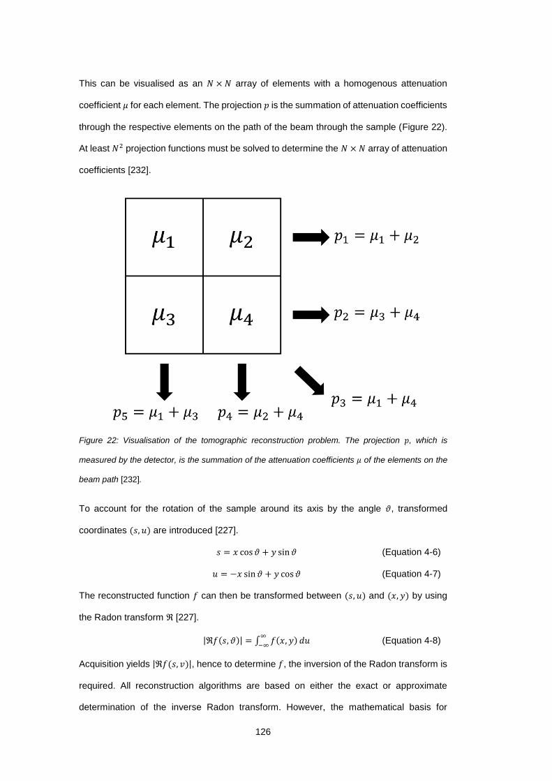
126
This can be visualised as an 𝑁 × 𝑁 array of elements with a homogenous attenuation
coefficient 𝜇 for each element. The projection 𝑝 is the summation of attenuation coefficients
through the respective elements on the path of the beam through the sample (Figure 22).
At least 𝑁2 projection functions must be solved to determine the 𝑁 × 𝑁 array of attenuation
coefficients [232].
Figure 22: Visualisation of the tomographic reconstruction problem. The projection 𝑝, which is
measured by the detector, is the summation of the attenuation coefficients 𝜇 of the elements on the
beam path [232].
To account for the rotation of the sample around its axis by the angle 𝜗, transformed
coordinates (𝑠, 𝑢) are introduced [227].
𝑠 = 𝑥 cos 𝜗 + 𝑦 sin 𝜗 (Equation 4-6)
𝑢 = −𝑥 sin 𝜗 + 𝑦 cos 𝜗 (Equation 4-7)
The reconstructed function 𝑓 can then be transformed between (𝑠, 𝑢) and (𝑥, 𝑦) by using
the Radon transform ℜ [227].
|ℜ𝑓(𝑠, 𝜗)| = ∫ 𝑓(𝑥, 𝑦)∞
−∞𝑑𝑢 (Equation 4-8)
Acquisition yields |ℜ𝑓(𝑠, 𝑣)|, hence to determine 𝑓, the inversion of the Radon transform is
required. All reconstruction algorithms are based on either the exact or approximate
determination of the inverse Radon transform. However, the mathematical basis for

127
obtaining this is beyond the scope of this work. The most commonly deployed solution for
the problem described above is the filtered back-projection algorithm [227].
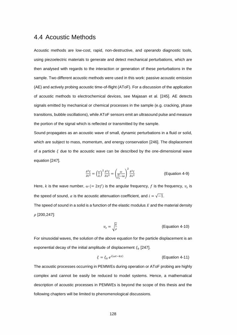
128
4.4 Acoustic Methods
Acoustic methods are low-cost, rapid, non-destructive, and operando diagnostic tools,
using piezoelectric materials to generate and detect mechanical perturbations, which are
then analysed with regards to the interaction or generation of these perturbations in the
sample. Two different acoustic methods were used in this work: passive acoustic emission
(AE) and actively probing acoustic time-of-flight (AToF). For a discussion of the application
of acoustic methods to electrochemical devices, see Majasan et al. [245]. AE detects
signals emitted by mechanical or chemical processes in the sample (e.g. cracking, phase
transitions, bubble oscillations), while AToF sensors emit an ultrasound pulse and measure
the portion of the signal which is reflected or transmitted by the sample.
Sound propagates as an acoustic wave of small, dynamic perturbations in a fluid or solid,
which are subject to mass, momentum, and energy conservation [246]. The displacement
of a particle 𝜉 due to the acoustic wave can be described by the one-dimensional wave
equation [247].
𝛿2𝜉
𝜕𝑡2 = (𝜔
𝑘)
2 𝛿2𝜉
𝜕𝑥2 = (𝜔
𝜔
𝑣𝑠−𝑖𝛼
)
2𝛿2𝜉
𝜕𝑥2 (Equation 4-9)
Here, 𝑘 is the wave number, 𝜔 (= 2𝜋𝑓) is the angular frequency, 𝑓 is the frequency, 𝑣𝑠 is
the speed of sound, 𝛼 is the acoustic attenuation coefficient, and 𝑖 = √−1.
The speed of sound in a solid is a function of the elastic modulus 𝐸 and the material density
𝜌 [200,247]:
𝑣𝑠 = √𝐸
𝜌 (Equation 4-10)
For sinusoidal waves, the solution of the above equation for the particle displacement is an
exponential decay of the initial amplitude of displacement 𝜉0 [247].
𝜉 = 𝜉0 𝑒𝑖(𝜔𝑡−𝑘𝑥) (Equation 4-11)
The acoustic processes occurring in PEMWEs during operation or AToF probing are highly
complex and cannot be easily be reduced to model systems. Hence, a mathematical
description of acoustic processes in PEMWEs is beyond the scope of this thesis and the
following chapters will be limited to phenomenological discussions.
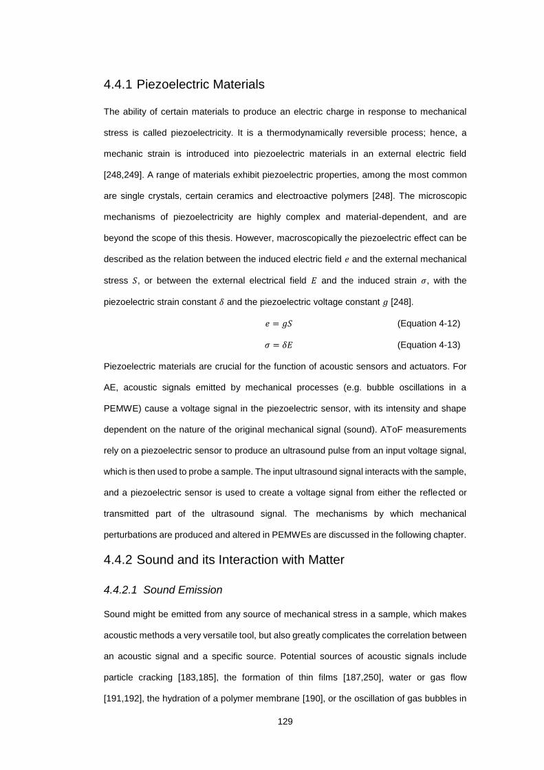
129
4.4.1 Piezoelectric Materials
The ability of certain materials to produce an electric charge in response to mechanical
stress is called piezoelectricity. It is a thermodynamically reversible process; hence, a
mechanic strain is introduced into piezoelectric materials in an external electric field
[248,249]. A range of materials exhibit piezoelectric properties, among the most common
are single crystals, certain ceramics and electroactive polymers [248]. The microscopic
mechanisms of piezoelectricity are highly complex and material-dependent, and are
beyond the scope of this thesis. However, macroscopically the piezoelectric effect can be
described as the relation between the induced electric field 𝑒 and the external mechanical
stress 𝑆, or between the external electrical field 𝐸 and the induced strain 𝜎, with the
piezoelectric strain constant 𝛿 and the piezoelectric voltage constant 𝑔 [248].
𝑒 = 𝑔𝑆 (Equation 4-12)
𝜎 = 𝛿𝐸 (Equation 4-13)
Piezoelectric materials are crucial for the function of acoustic sensors and actuators. For
AE, acoustic signals emitted by mechanical processes (e.g. bubble oscillations in a
PEMWE) cause a voltage signal in the piezoelectric sensor, with its intensity and shape
dependent on the nature of the original mechanical signal (sound). AToF measurements
rely on a piezoelectric sensor to produce an ultrasound pulse from an input voltage signal,
which is then used to probe a sample. The input ultrasound signal interacts with the sample,
and a piezoelectric sensor is used to create a voltage signal from either the reflected or
transmitted part of the ultrasound signal. The mechanisms by which mechanical
perturbations are produced and altered in PEMWEs are discussed in the following chapter.
4.4.2 Sound and its Interaction with Matter
4.4.2.1 Sound Emission
Sound might be emitted from any source of mechanical stress in a sample, which makes
acoustic methods a very versatile tool, but also greatly complicates the correlation between
an acoustic signal and a specific source. Potential sources of acoustic signals include
particle cracking [183,185], the formation of thin films [187,250], water or gas flow
[191,192], the hydration of a polymer membrane [190], or the oscillation of gas bubbles in
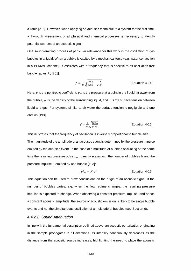
130
a liquid [218]. However, when applying an acoustic technique to a system for the first time,
a thorough assessment of all physical and chemical processes is necessary to identify
potential sources of an acoustic signal.
One sound-emitting process of particular relevance for this work is the oscillation of gas
bubbles in a liquid. When a bubble is excited by a mechanical force (e.g. water convection
in a PEMWE channel), it oscillates with a frequency that is specific to its oscillation-free
bubble radius 𝑅0 [251].
𝑓 =1
2𝜋√
3𝛾𝑝∞
𝜌𝑙𝑅02 −
2𝜎
𝜌𝑙𝑅03 (Equation 4-14)
Here, 𝛾 is the polytropic coefficient, 𝑝∞ is the pressure at a point in the liquid far away from
the bubble, 𝜌𝑙 is the density of the surrounding liquid, and 𝜎 is the surface tension between
liquid and gas. For systems similar to air-water the surface tension is negligible and one
obtains [193].
𝑓 =1
2𝜋√
3𝛾𝑝∞
𝜌𝑙𝑅02 (Equation 4-15)
This illustrates that the frequency of oscillation is inversely proportional to bubble size.
The magnitude of the amplitude of an acoustic event is determined by the pressure impulse
emitted by the acoustic event. In the case of a multitude of bubbles oscillating at the same
time the resulting pressure pulse 𝑝𝑟𝑒𝑠 directly scales with the number of bubbles 𝑁 and the
pressure impulse 𝑝 emitted by one bubble [193]:
𝑝𝑟𝑒𝑠2 = 𝑁 𝑝2 (Equation 4-16)
This equation can be used to draw conclusions on the origin of an acoustic signal. If the
number of bubbles varies, e.g. when the flow regime changes, the resulting pressure
impulse is expected to change. When observing a constant pressure impulse, and hence
a constant acoustic amplitude, the source of acoustic emission is likely to be single bubble
events and not the simultaneous oscillation of a multitude of bubbles (see Section 6).
4.4.2.2 Sound Attenuation
In line with the fundamental description outlined above, an acoustic perturbation originating
in the sample propagates in all directions. Its intensity continuously decreases as the
distance from the acoustic source increases, highlighting the need to place the acoustic
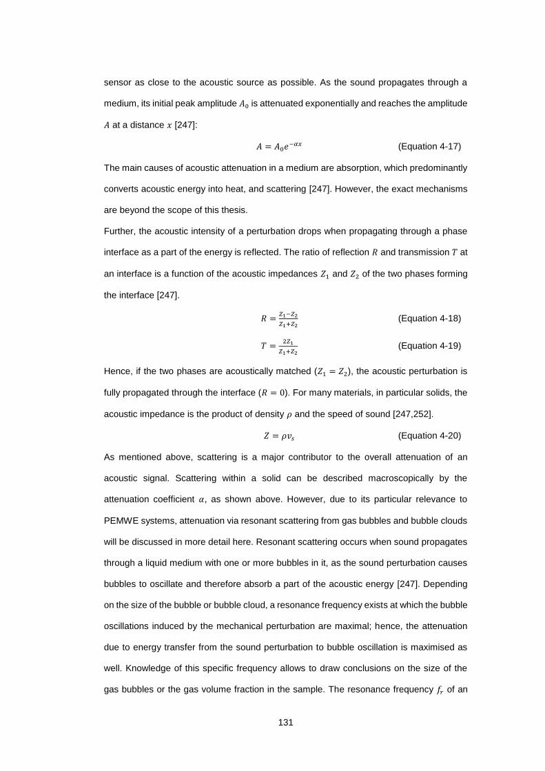
131
sensor as close to the acoustic source as possible. As the sound propagates through a
medium, its initial peak amplitude 𝐴0 is attenuated exponentially and reaches the amplitude
𝐴 at a distance 𝑥 [247]:
𝐴 = 𝐴0𝑒−𝛼𝑥 (Equation 4-17)
The main causes of acoustic attenuation in a medium are absorption, which predominantly
converts acoustic energy into heat, and scattering [247]. However, the exact mechanisms
are beyond the scope of this thesis.
Further, the acoustic intensity of a perturbation drops when propagating through a phase
interface as a part of the energy is reflected. The ratio of reflection 𝑅 and transmission 𝑇 at
an interface is a function of the acoustic impedances 𝑍1 and 𝑍2 of the two phases forming
the interface [247].
𝑅 =𝑍1−𝑍2
𝑍1+𝑍2 (Equation 4-18)
𝑇 =2𝑍1
𝑍1+𝑍2 (Equation 4-19)
Hence, if the two phases are acoustically matched (𝑍1 = 𝑍2), the acoustic perturbation is
fully propagated through the interface (𝑅 = 0). For many materials, in particular solids, the
acoustic impedance is the product of density 𝜌 and the speed of sound [247,252].
𝑍 = 𝜌𝑣𝑠 (Equation 4-20)
As mentioned above, scattering is a major contributor to the overall attenuation of an
acoustic signal. Scattering within a solid can be described macroscopically by the
attenuation coefficient 𝛼, as shown above. However, due to its particular relevance to
PEMWE systems, attenuation via resonant scattering from gas bubbles and bubble clouds
will be discussed in more detail here. Resonant scattering occurs when sound propagates
through a liquid medium with one or more bubbles in it, as the sound perturbation causes
bubbles to oscillate and therefore absorb a part of the acoustic energy [247]. Depending
on the size of the bubble or bubble cloud, a resonance frequency exists at which the bubble
oscillations induced by the mechanical perturbation are maximal; hence, the attenuation
due to energy transfer from the sound perturbation to bubble oscillation is maximised as
well. Knowledge of this specific frequency allows to draw conclusions on the size of the
gas bubbles or the gas volume fraction in the sample. The resonance frequency 𝑓𝑟 of an
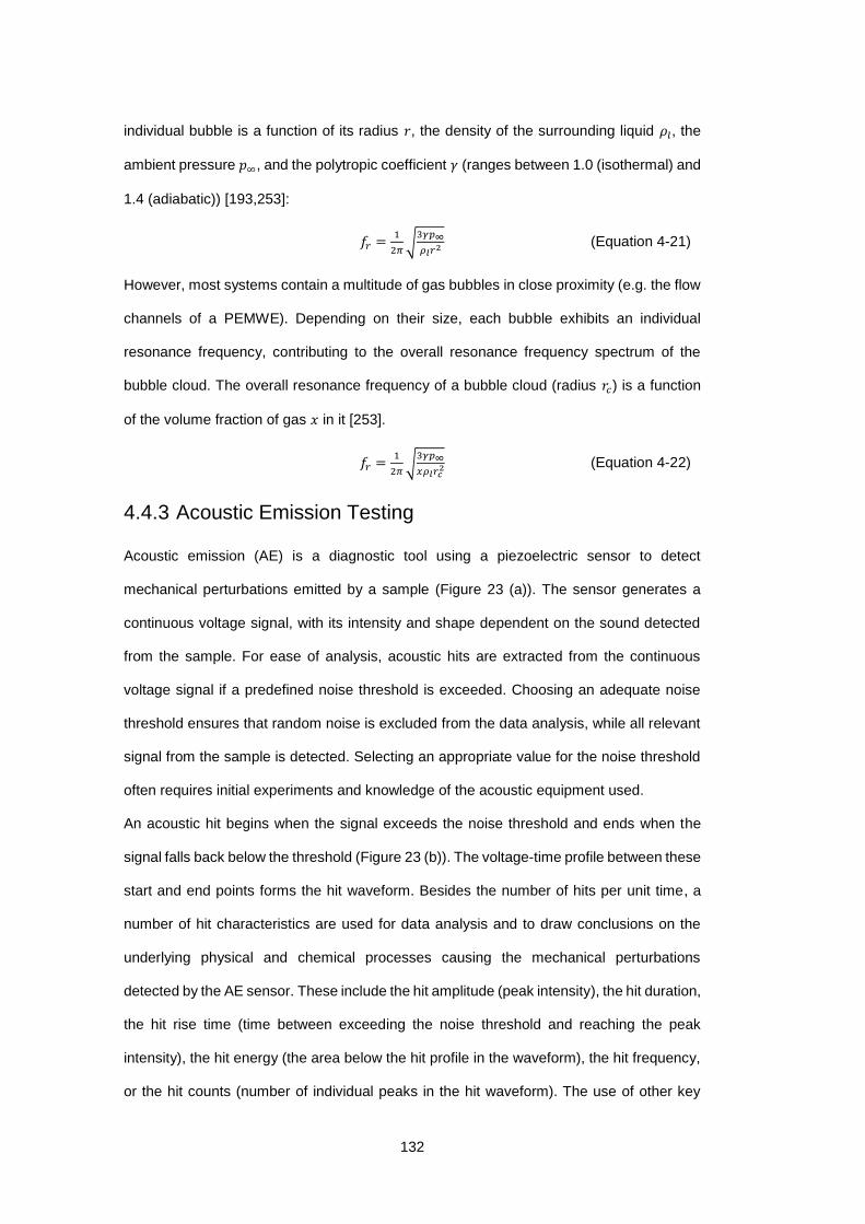
132
individual bubble is a function of its radius 𝑟, the density of the surrounding liquid 𝜌𝑙, the
ambient pressure 𝑝∞, and the polytropic coefficient 𝛾 (ranges between 1.0 (isothermal) and
1.4 (adiabatic)) [193,253]:
𝑓𝑟 =1
2𝜋√
3𝛾𝑝∞
𝜌𝑙𝑟2 (Equation 4-21)
However, most systems contain a multitude of gas bubbles in close proximity (e.g. the flow
channels of a PEMWE). Depending on their size, each bubble exhibits an individual
resonance frequency, contributing to the overall resonance frequency spectrum of the
bubble cloud. The overall resonance frequency of a bubble cloud (radius 𝑟𝑐) is a function
of the volume fraction of gas 𝑥 in it [253].
𝑓𝑟 =1
2𝜋√
3𝛾𝑝∞
𝑥𝜌𝑙𝑟𝑐2 (Equation 4-22)
4.4.3 Acoustic Emission Testing
Acoustic emission (AE) is a diagnostic tool using a piezoelectric sensor to detect
mechanical perturbations emitted by a sample (Figure 23 (a)). The sensor generates a
continuous voltage signal, with its intensity and shape dependent on the sound detected
from the sample. For ease of analysis, acoustic hits are extracted from the continuous
voltage signal if a predefined noise threshold is exceeded. Choosing an adequate noise
threshold ensures that random noise is excluded from the data analysis, while all relevant
signal from the sample is detected. Selecting an appropriate value for the noise threshold
often requires initial experiments and knowledge of the acoustic equipment used.
An acoustic hit begins when the signal exceeds the noise threshold and ends when the
signal falls back below the threshold (Figure 23 (b)). The voltage-time profile between these
start and end points forms the hit waveform. Besides the number of hits per unit time, a
number of hit characteristics are used for data analysis and to draw conclusions on the
underlying physical and chemical processes causing the mechanical perturbations
detected by the AE sensor. These include the hit amplitude (peak intensity), the hit duration,
the hit rise time (time between exceeding the noise threshold and reaching the peak
intensity), the hit energy (the area below the hit profile in the waveform), the hit frequency,
or the hit counts (number of individual peaks in the hit waveform). The use of other key
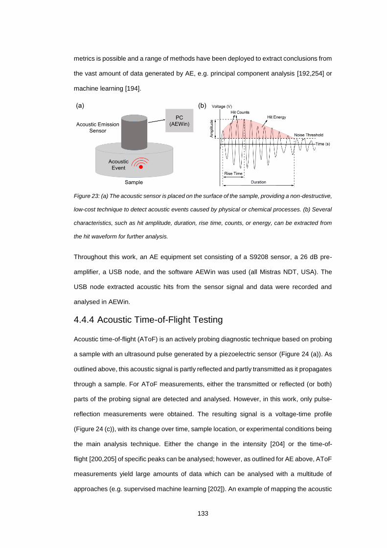
133
metrics is possible and a range of methods have been deployed to extract conclusions from
the vast amount of data generated by AE, e.g. principal component analysis [192,254] or
machine learning [194].
Figure 23: (a) The acoustic sensor is placed on the surface of the sample, providing a non-destructive,
low-cost technique to detect acoustic events caused by physical or chemical processes. (b) Several
characteristics, such as hit amplitude, duration, rise time, counts, or energy, can be extracted from
the hit waveform for further analysis.
Throughout this work, an AE equipment set consisting of a S9208 sensor, a 26 dB pre-
amplifier, a USB node, and the software AEWin was used (all Mistras NDT, USA). The
USB node extracted acoustic hits from the sensor signal and data were recorded and
analysed in AEWin.
4.4.4 Acoustic Time-of-Flight Testing
Acoustic time-of-flight (AToF) is an actively probing diagnostic technique based on probing
a sample with an ultrasound pulse generated by a piezoelectric sensor (Figure 24 (a)). As
outlined above, this acoustic signal is partly reflected and partly transmitted as it propagates
through a sample. For AToF measurements, either the transmitted or reflected (or both)
parts of the probing signal are detected and analysed. However, in this work, only pulse-
reflection measurements were obtained. The resulting signal is a voltage-time profile
(Figure 24 (c)), with its change over time, sample location, or experimental conditions being
the main analysis technique. Either the change in the intensity [204] or the time-of-
flight [200,205] of specific peaks can be analysed; however, as outlined for AE above, AToF
measurements yield large amounts of data which can be analysed with a multitude of
approaches (e.g. supervised machine learning [202]). An example of mapping the acoustic
134
reflection intensity across the sensor width as a function of time is shown in Figure 24 (d).
The AToF measurements in this work were taken with an acoustic array of 64 individual
sensors (Figure 24 (b)), with every measurement being the average from a ‘sensor unit’
(16 adjacent sensors). Every sensor generated an input pulse frequency with a maximum
repetition frequency of 20 kHz and measured the reflected signal (pulse-echo mode). The
acoustic array was controlled and data recorded with an Olympus FOCUS PX system
(Olympus Scientific Solutions, USA). A thin layer of acoustic gel (D12 Couplant Gel,
Olympus Scientific Solutions, USA) was applied to the surface of the acoustic array before
experiments to maximise the transmission of the probing signal into the PEMWE. The
FocusPC software (Olympus Scientific Solutions, USA) was used for real-time data
visualisation and export.
Figure 24: (a) The AToF sensor array consisting of 64 individual sensors is placed on the sample
surface. It emits an acoustic pulse into the sample and measures the reflected signal. (b) For each
measurement, the measured reflection signal from 16 adjacent sensors is averaged, resulting in (c)
an acoustic waveform. A specific peak or time-of-flight interval is then selected and the maximum
peak intensity in this interval is measured. (d) By mapping this maximum intensity across all units of
16 sensors (sensor unit) and another experimental variable (e.g. time), detailed information on
processes in the sample can be obtained.
135
4.5 Fast Fourier Transform
Fourier transformation is a method of obtaining the frequency spectrum of a time series,
e.g. a voltage-time profile. To analyse discretely sampled data the discrete Fourier
transform is used, with the fast Fourier transform (FFT) being an especially efficient solution
of the discrete Fourier transform [255,256]. The mathematical foundations of the FFT are
beyond the scope of this thesis, but it was used to analyse data obtained with acoustic
emission (AE) and acoustic time-of-flight (AToF) imaging. The frequency of individual AE
hits was determined in AEWin, while the frequency of pulse-echo AToF waveforms was
measured using the FocusPC software.
136
4.6 Conclusions
This work employs imaging-based techniques to gain insight into the water-gas distribution
in the LGDL and flow channels; however, due to cost and accessibility concerns afflicted
to neutron imaging, acoustic diagnostic tools are introduced to investigate mass transport
processes in PEMWEs. Hence, this section described the underpinnings of these
techniques, enabling a thorough understanding of the experimental results presented later.
The underlying mechanisms of X-ray and neutron production for imaging, the interactions
of photons and neutrons with matter, and the acquisition and detection of photons and
neutrons were outlined. A brief description of tomographic reconstruction of two-
dimensional data sets into a three-dimensional sample representation was given.
Lastly, the fundamentals of wave theory were described, followed by a discussion of the
interaction of sound with matter, and piezoelectric materials, which are crucial for acoustic
diagnostic methods.
137
5 The Influence of Liquid-Gas Diffusion Layer Microstructure on the Water-Gas Distribution

139
5.1 Overview
In this chapter, neutron radiography is deployed to measure the spatial distribution of water
within three different LGDLs, while X-ray micro-computed tomography (XCT) is used to
characterize the microstructure of the LGDL materials. The combination of these two
techniques yields valuable insight into water transport within the LGDL and the influence
of microstructure on the water-gas distribution. Significant local water heterogeneity is
observed and results suggest a link between flow-field geometry/location and LGDL mass
transport. It is further shown that the pore volume in these LGDLs is significantly under-
utilized, pointing the way towards design optimisation of LGDL materials and architectures.
The work in this chapter has been published in Journal of Power Sources [90].
140
5.2 Introduction
The ability of neutrons to penetrate many materials with a high molecular mass, while being
strongly attenuated by specific light materials, such as hydrogen and lithium, makes
neutron imaging a powerful tool for visualizing water distribution in PEMWEs. By combining
neutron imaging with X-ray micro-computed tomography (XCT) the water-gas distribution
in the LGDL can be related to its microstructure.
This chapter uses operando through-plane neutron radiography of PEMWEs at current
densities of up to 1.5 A cm-2 to examine mass transport of water within LGDLs under rib
(land) locations. As outlined in Section 5.3.1, the PEMWE cell used in these experiments
used aluminium components to maximise neutron transmission, however, this led to
reduced electrochemical performance. Hence, to avoid excessive voltages, the PEMWE
cell was only operated up to 1.5 A cm-2. Three different LGDL materials, one sintered
powder, and two fibrous materials, are investigated and XCT is employed to link the
microstructure of the LGDL to its mass transport and the water saturation in the LGDL
pores.
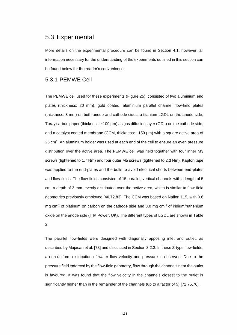
141
5.3 Experimental
More details on the experimental procedure can be found in Section 4.1; however, all
information necessary for the understanding of the experiments outlined in this section can
be found below for the reader’s convenience.
5.3.1 PEMWE Cell
The PEMWE cell used for these experiments (Figure 25), consisted of two aluminium end
plates (thickness: 20 mm), gold coated, aluminium parallel channel flow-field plates
(thickness: 3 mm) on both anode and cathode sides, a titanium LGDL on the anode side,
Toray carbon paper (thickness: ~100 µm) as gas diffusion layer (GDL) on the cathode side,
and a catalyst coated membrane (CCM, thickness: ~150 µm) with a square active area of
25 cm2. An aluminium holder was used at each end of the cell to ensure an even pressure
distribution over the active area. The PEMWE cell was held together with four inner M3
screws (tightened to 1.7 Nm) and four outer M5 screws (tightened to 2.3 Nm). Kapton tape
was applied to the end-plates and the bolts to avoid electrical shorts between end-plates
and flow-fields. The flow-fields consisted of 15 parallel, vertical channels with a length of 5
cm, a depth of 3 mm, evenly distributed over the active area, which is similar to flow-field
geometries previously employed [40,72,83]. The CCM was based on Nafion 115, with 0.6
mg cm-2 of platinum on carbon on the cathode side and 3.0 mg cm-2 of iridium/ruthenium
oxide on the anode side (ITM Power, UK). The different types of LGDL are shown in Table
2.
The parallel flow-fields were designed with diagonally opposing inlet and outlet, as
described by Majasan et al. [73] and discussed in Section 3.2.3. In these Z-type flow-fields,
a non-uniform distribution of water flow velocity and pressure is observed. Due to the
pressure field enforced by the flow-field geometry, flow through the channels near the outlet
is favoured. It was found that the flow velocity in the channels closest to the outlet is
significantly higher than in the remainder of the channels (up to a factor of 5) [72,75,76].
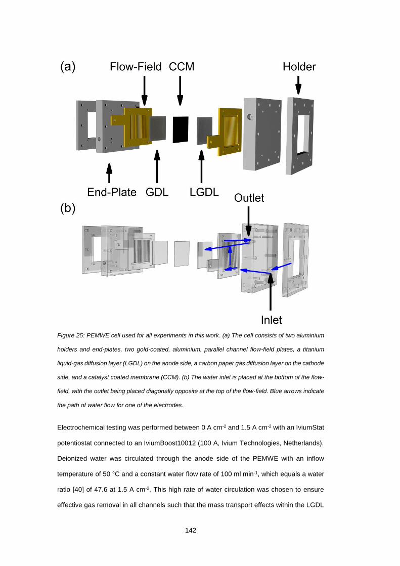
142
Figure 25: PEMWE cell used for all experiments in this work. (a) The cell consists of two aluminium
holders and end-plates, two gold-coated, aluminium, parallel channel flow-field plates, a titanium
liquid-gas diffusion layer (LGDL) on the anode side, a carbon paper gas diffusion layer on the cathode
side, and a catalyst coated membrane (CCM). (b) The water inlet is placed at the bottom of the flow-
field, with the outlet being placed diagonally opposite at the top of the flow-field. Blue arrows indicate
the path of water flow for one of the electrodes.
Electrochemical testing was performed between 0 A cm-2 and 1.5 A cm-2 with an IviumStat
potentiostat connected to an IviumBoost10012 (100 A, Ivium Technologies, Netherlands).
Deionized water was circulated through the anode side of the PEMWE with an inflow
temperature of 50 °C and a constant water flow rate of 100 ml min-1, which equals a water
ratio [40] of 47.6 at 1.5 A cm-2. This high rate of water circulation was chosen to ensure
effective gas removal in all channels such that the mass transport effects within the LGDL
143
could be highlighted. The cathode side was run dry without water inflow.
Table 2: Description, thickness, and supplier of the three LGDLs used in this chapter. The ID will be
used in the text to refer to a specific LGDL.
ID Description Thickness (mm) Supplier
Sinter Sintered titanium
particles
2.0 Merelex (USA)
Thick Felt Sintered titanium fibres 1.0 NIKKO Techno (Japan)
Thin Felt Sintered titanium fibres 0.1 NIKKO Techno (Japan)
5.3.2 Neutron Imaging and Imaging Analysis
Neutron radiography was carried out at the Cold Neutron Tomography and Radiography
beamline V7 (CONRAD) at Helmholtz-Zentrum Berlin, Germany. For every set of
conditions, 30 through-plane images were taken with an exposure time of 5 s. For the
detector system [242] a pixel size of 23.9 µm with a corresponding total field-of-view of 49
x 49 mm was set. Before starting an experiment with a specific LGDL, images without
neutron beam (dark-field) and of the PEMWE cell before water was pumped through it (dry
image) were taken (30 images each, 5 s exposure).
All images were then analysed using ImageJ (Fiji, Version 1.52p). Outliers were removed
from all images (Radius: 2 pixels, Threshold: 50). Then each set of 30 images (PEMWE
cell, dark-field, dry images) was median averaged and the dark-field was subtracted. These
images were then normalized by dividing by the dry image. This accounts for dead pixels
on the detector, the locally varying intensity of the neutron beam and also removes the
contributions from PEMWE components which remain unchanged during operation (end
plates, flow-fields, and titanium in the LGDL). The greyscale value was converted to a water
thickness using the Beer-Lambert law [154,238]. The distance between PEMWE cell and
detector was 10 cm, which reduced the effect of neutron scattering and therefore improved
144
the accuracy of the quantification of water thickness. For this distance between cell and
detector, the attenuation coefficient of neutrons in water was 5.2 cm-1, as provided by the
beamline. Details on the image analysis can be found in Section 4.3.2.4 and Figure 20.
The purpose of this study is to examine the water/gas composition within the LGDL. To do
this, the land locations are focused on as the open flow channels are dominated by
relatively unstable two-phase flow with time-varying bubble dynamics, which precludes
accurate analysis of the effective water thickness in the LGDL. Indeed, flow dynamics within
channels have been extensively studied using optical cells [43,44,73,218], but it is the
particular ability of neutron imaging to examine water under lands and within porous
structures that is exploited here [87,88].
A potential limitation of the through-plane measurement technique is that the results for the
water thickness are a summation of water through the anode, cathode and membrane
components. This is another reason the water thickness is only quantified for the rib (‘land’)
areas. However, as the CCM was fully hydrated before the experiments and remains so
throughout these experiments, and the CCM and carbon paper are relatively thin, water in
the LGDL of the anode side will dominate the neutron absorption response.
5.3.3 X-ray Micro-Computed tomography
X-ray computed tomograms were acquired for all LGDL materials used in this chapter. The
Zeiss Xradia Versa 520 (Carl Zeiss X-ray Microscopy Inc., Pleasanton, CA) lab-based X-
ray system was used to acquire the XCT datasets. The acquisition parameters are
summarized in Table 3. Radiographic images were reconstructed into tomograms with the
Zeiss Scout-and-Scan Control System Reconstructor software. Volume renderings were
generated and analysed using Avizo (Thermo Fisher Scientific, US), which is a well-
established tool for the segmentation and analysis of XCT datasets of porous media [257–
259]. The greyscale tomograms were then segmented using a manual threshold method
according to the greyscale value. The porosity of the sample was calculated from this
segmentation. Avizo was then used to create a pore network model (and the related pore
size distribution), from which the flux of water at 50 °C through the LGDL with an input
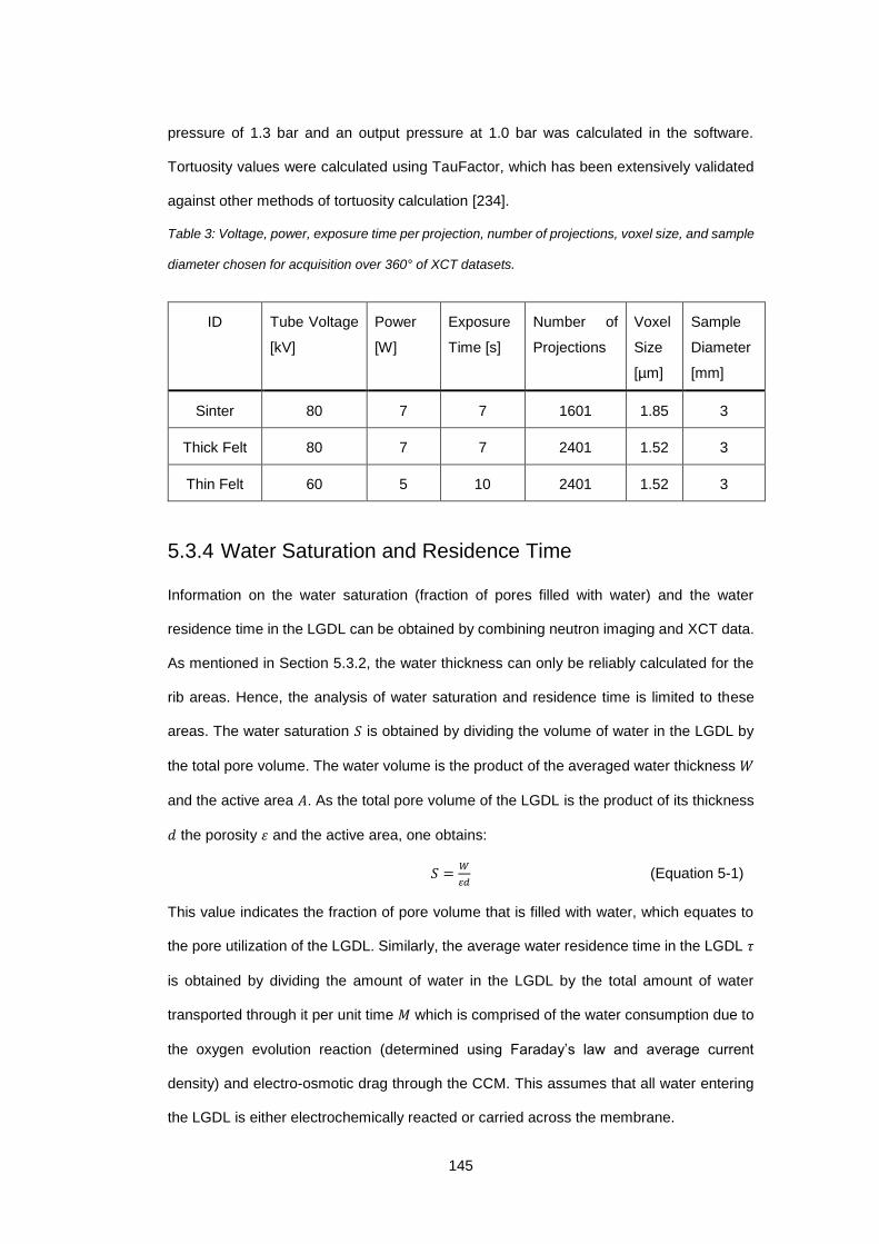
145
pressure of 1.3 bar and an output pressure at 1.0 bar was calculated in the software.
Tortuosity values were calculated using TauFactor, which has been extensively validated
against other methods of tortuosity calculation [234].
Table 3: Voltage, power, exposure time per projection, number of projections, voxel size, and sample
diameter chosen for acquisition over 360° of XCT datasets.
ID Tube Voltage
[kV]
Power
[W]
Exposure
Time [s]
Number of
Projections
Voxel
Size
[µm]
Sample
Diameter
[mm]
Sinter 80 7 7 1601 1.85 3
Thick Felt 80 7 7 2401 1.52 3
Thin Felt 60 5 10 2401 1.52 3
5.3.4 Water Saturation and Residence Time
Information on the water saturation (fraction of pores filled with water) and the water
residence time in the LGDL can be obtained by combining neutron imaging and XCT data.
As mentioned in Section 5.3.2, the water thickness can only be reliably calculated for the
rib areas. Hence, the analysis of water saturation and residence time is limited to these
areas. The water saturation 𝑆 is obtained by dividing the volume of water in the LGDL by
the total pore volume. The water volume is the product of the averaged water thickness 𝑊
and the active area 𝐴. As the total pore volume of the LGDL is the product of its thickness
𝑑 the porosity 휀 and the active area, one obtains:
𝑆 =𝑊
𝑑 (Equation 5-1)
This value indicates the fraction of pore volume that is filled with water, which equates to
the pore utilization of the LGDL. Similarly, the average water residence time in the LGDL 𝜏
is obtained by dividing the amount of water in the LGDL by the total amount of water
transported through it per unit time 𝑀 which is comprised of the water consumption due to
the oxygen evolution reaction (determined using Faraday’s law and average current
density) and electro-osmotic drag through the CCM. This assumes that all water entering
the LGDL is either electrochemically reacted or carried across the membrane.

146
𝜏 =𝜌𝑊𝐴
𝑀 (Equation 5-2)
Details on the calculation of these mass flows were described by Ito et al. [40,41] and can
be found in Section 3.2.2. 𝑀 is typically a gravimetric value, hence the density of water 𝜌
is used to convert 𝜏 into a volumetric value.
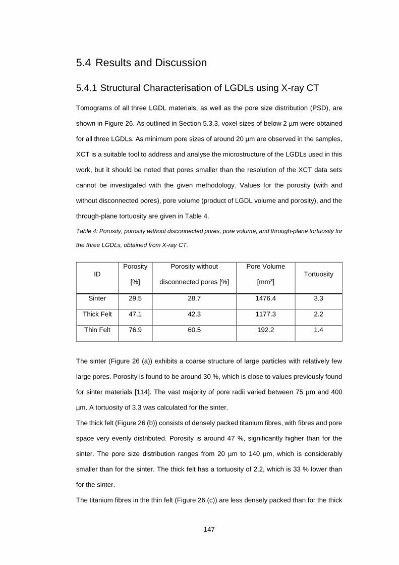
147
5.4 Results and Discussion
5.4.1 Structural Characterisation of LGDLs using X-ray CT
Tomograms of all three LGDL materials, as well as the pore size distribution (PSD), are
shown in Figure 26. As outlined in Section 5.3.3, voxel sizes of below 2 µm were obtained
for all three LGDLs. As minimum pore sizes of around 20 µm are observed in the samples,
XCT is a suitable tool to address and analyse the microstructure of the LGDLs used in this
work, but it should be noted that pores smaller than the resolution of the XCT data sets
cannot be investigated with the given methodology. Values for the porosity (with and
without disconnected pores), pore volume (product of LGDL volume and porosity), and the
through-plane tortuosity are given in Table 4.
Table 4: Porosity, porosity without disconnected pores, pore volume, and through-plane tortuosity for
the three LGDLs, obtained from X-ray CT.
ID Porosity
[%]
Porosity without
disconnected pores [%]
Pore Volume
[mm3] Tortuosity
Sinter 29.5 28.7 1476.4 3.3
Thick Felt 47.1 42.3 1177.3 2.2
Thin Felt 76.9 60.5 192.2 1.4
The sinter (Figure 26 (a)) exhibits a coarse structure of large particles with relatively few
large pores. Porosity is found to be around 30 %, which is close to values previously found
for sinter materials [114]. The vast majority of pore radii varied between 75 µm and 400
µm. A tortuosity of 3.3 was calculated for the sinter.
The thick felt (Figure 26 (b)) consists of densely packed titanium fibres, with fibres and pore
space very evenly distributed. Porosity is around 47 %, significantly higher than for the
sinter. The pore size distribution ranges from 20 µm to 140 µm, which is considerably
smaller than for the sinter. The thick felt has a tortuosity of 2.2, which is 33 % lower than
for the sinter.
The titanium fibres in the thin felt (Figure 26 (c)) are less densely packed than for the thick
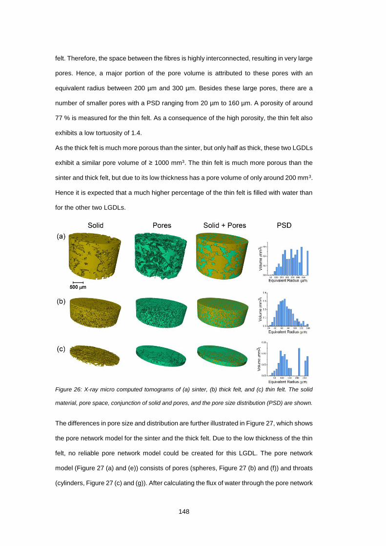
148
felt. Therefore, the space between the fibres is highly interconnected, resulting in very large
pores. Hence, a major portion of the pore volume is attributed to these pores with an
equivalent radius between 200 µm and 300 µm. Besides these large pores, there are a
number of smaller pores with a PSD ranging from 20 µm to 160 µm. A porosity of around
77 % is measured for the thin felt. As a consequence of the high porosity, the thin felt also
exhibits a low tortuosity of 1.4.
As the thick felt is much more porous than the sinter, but only half as thick, these two LGDLs
exhibit a similar pore volume of ≥ 1000 mm3. The thin felt is much more porous than the
sinter and thick felt, but due to its low thickness has a pore volume of only around 200 mm3.
Hence it is expected that a much higher percentage of the thin felt is filled with water than
for the other two LGDLs.
Figure 26: X-ray micro computed tomograms of (a) sinter, (b) thick felt, and (c) thin felt. The solid
material, pore space, conjunction of solid and pores, and the pore size distribution (PSD) are shown.
The differences in pore size and distribution are further illustrated in Figure 27, which shows
the pore network model for the sinter and the thick felt. Due to the low thickness of the thin
felt, no reliable pore network model could be created for this LGDL. The pore network
model (Figure 27 (a) and (e)) consists of pores (spheres, Figure 27 (b) and (f)) and throats
(cylinders, Figure 27 (c) and (g)). After calculating the flux of water through the pore network
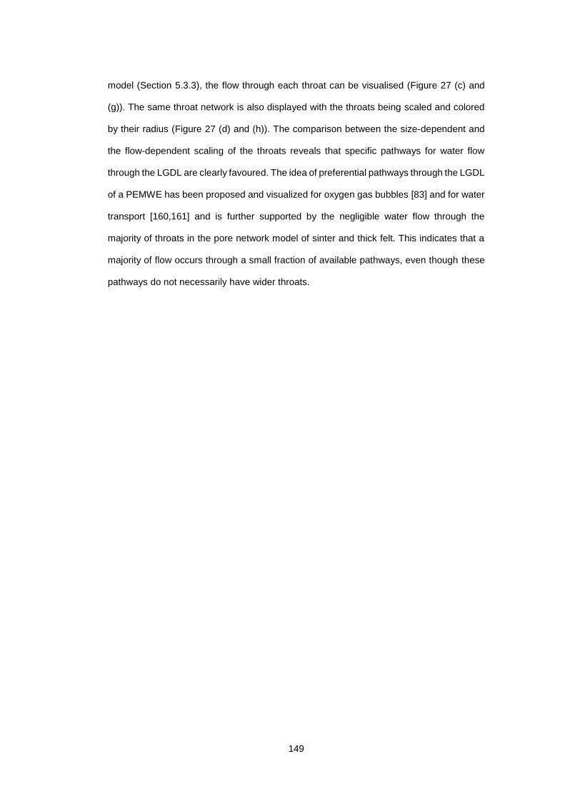
149
model (Section 5.3.3), the flow through each throat can be visualised (Figure 27 (c) and
(g)). The same throat network is also displayed with the throats being scaled and colored
by their radius (Figure 27 (d) and (h)). The comparison between the size-dependent and
the flow-dependent scaling of the throats reveals that specific pathways for water flow
through the LGDL are clearly favoured. The idea of preferential pathways through the LGDL
of a PEMWE has been proposed and visualized for oxygen gas bubbles [83] and for water
transport [160,161] and is further supported by the negligible water flow through the
majority of throats in the pore network model of sinter and thick felt. This indicates that a
majority of flow occurs through a small fraction of available pathways, even though these
pathways do not necessarily have wider throats.
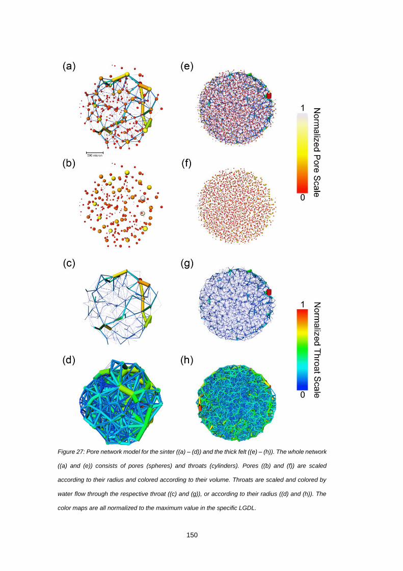
150
Figure 27: Pore network model for the sinter ((a) – (d)) and the thick felt ((e) – (h)). The whole network
((a) and (e)) consists of pores (spheres) and throats (cylinders). Pores ((b) and (f)) are scaled
according to their radius and colored according to their volume. Throats are scaled and colored by
water flow through the respective throat ((c) and (g)), or according to their radius ((d) and (h)). The
color maps are all normalized to the maximum value in the specific LGDL.
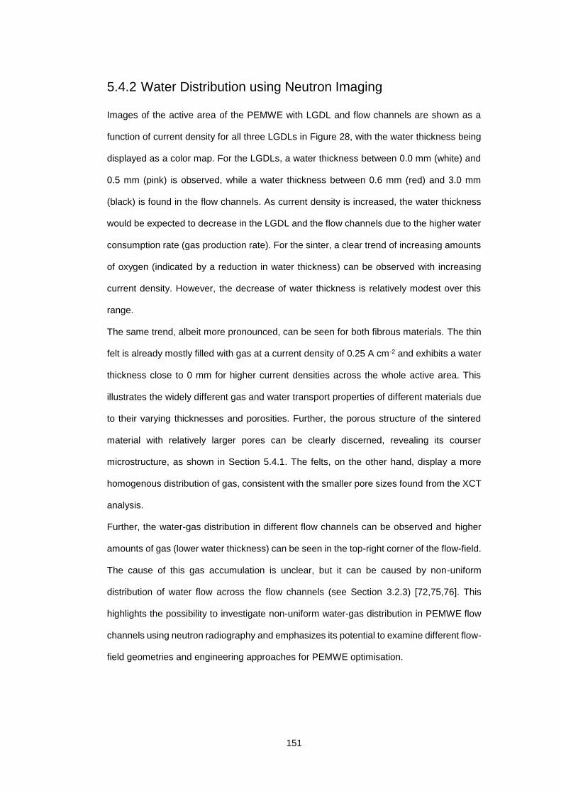
151
5.4.2 Water Distribution using Neutron Imaging
Images of the active area of the PEMWE with LGDL and flow channels are shown as a
function of current density for all three LGDLs in Figure 28, with the water thickness being
displayed as a color map. For the LGDLs, a water thickness between 0.0 mm (white) and
0.5 mm (pink) is observed, while a water thickness between 0.6 mm (red) and 3.0 mm
(black) is found in the flow channels. As current density is increased, the water thickness
would be expected to decrease in the LGDL and the flow channels due to the higher water
consumption rate (gas production rate). For the sinter, a clear trend of increasing amounts
of oxygen (indicated by a reduction in water thickness) can be observed with increasing
current density. However, the decrease of water thickness is relatively modest over this
range.
The same trend, albeit more pronounced, can be seen for both fibrous materials. The thin
felt is already mostly filled with gas at a current density of 0.25 A cm-2 and exhibits a water
thickness close to 0 mm for higher current densities across the whole active area. This
illustrates the widely different gas and water transport properties of different materials due
to their varying thicknesses and porosities. Further, the porous structure of the sintered
material with relatively larger pores can be clearly discerned, revealing its courser
microstructure, as shown in Section 5.4.1. The felts, on the other hand, display a more
homogenous distribution of gas, consistent with the smaller pore sizes found from the XCT
analysis.
Further, the water-gas distribution in different flow channels can be observed and higher
amounts of gas (lower water thickness) can be seen in the top-right corner of the flow-field.
The cause of this gas accumulation is unclear, but it can be caused by non-uniform
distribution of water flow across the flow channels (see Section 3.2.3) [72,75,76]. This
highlights the possibility to investigate non-uniform water-gas distribution in PEMWE flow
channels using neutron radiography and emphasizes its potential to examine different flow-
field geometries and engineering approaches for PEMWE optimisation.
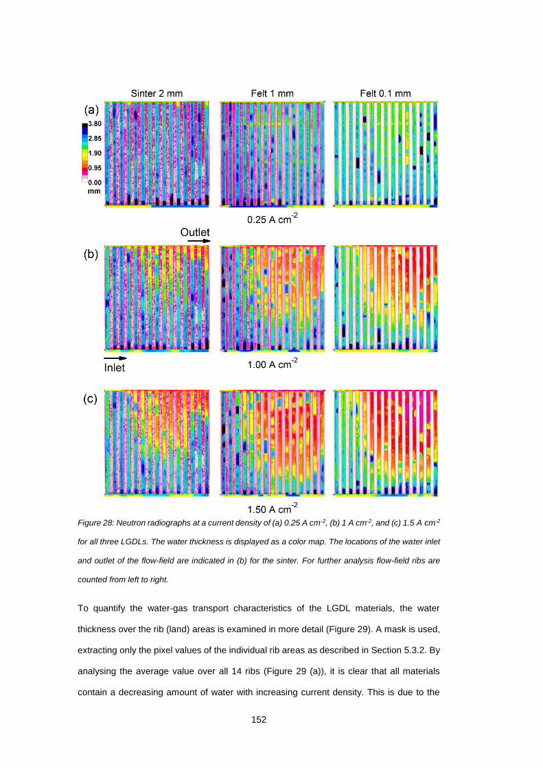
152
Figure 28: Neutron radiographs at a current density of (a) 0.25 A cm-2, (b) 1 A cm-2, and (c) 1.5 A cm-2
for all three LGDLs. The water thickness is displayed as a color map. The locations of the water inlet
and outlet of the flow-field are indicated in (b) for the sinter. For further analysis flow-field ribs are
counted from left to right.
To quantify the water-gas transport characteristics of the LGDL materials, the water
thickness over the rib (land) areas is examined in more detail (Figure 29). A mask is used,
extracting only the pixel values of the individual rib areas as described in Section 5.3.2. By
analysing the average value over all 14 ribs (Figure 29 (a)), it is clear that all materials
contain a decreasing amount of water with increasing current density. This is due to the
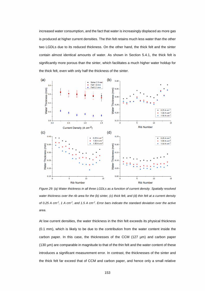
153
increased water consumption, and the fact that water is increasingly displaced as more gas
is produced at higher current densities. The thin felt retains much less water than the other
two LGDLs due to its reduced thickness. On the other hand, the thick felt and the sinter
contain almost identical amounts of water. As shown in Section 5.4.1, the thick felt is
significantly more porous than the sinter, which facilitates a much higher water holdup for
the thick felt, even with only half the thickness of the sinter.
Figure 29: (a) Water thickness in all three LGDLs as a function of current density. Spatially resolved
water thickness over the rib area for the (b) sinter, (c) thick felt, and (d) thin felt at a current density
of 0.25 A cm-2, 1 A cm-2, and 1.5 A cm-2. Error bars indicate the standard deviation over the active
area.
At low current densities, the water thickness in the thin felt exceeds its physical thickness
(0.1 mm), which is likely to be due to the contribution from the water content inside the
carbon paper. In this case, the thicknesses of the CCM (127 µm) and carbon paper
(130 µm) are comparable in magnitude to that of the thin felt and the water content of these
introduces a significant measurement error. In contrast, the thicknesses of the sinter and
the thick felt far exceed that of CCM and carbon paper, and hence only a small relative
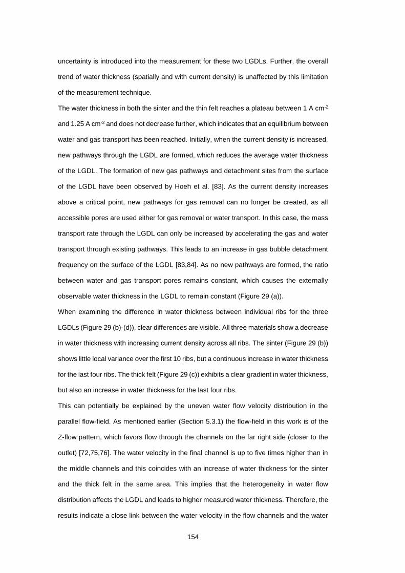
154
uncertainty is introduced into the measurement for these two LGDLs. Further, the overall
trend of water thickness (spatially and with current density) is unaffected by this limitation
of the measurement technique.
The water thickness in both the sinter and the thin felt reaches a plateau between 1 A cm-2
and 1.25 A cm-2 and does not decrease further, which indicates that an equilibrium between
water and gas transport has been reached. Initially, when the current density is increased,
new pathways through the LGDL are formed, which reduces the average water thickness
of the LGDL. The formation of new gas pathways and detachment sites from the surface
of the LGDL have been observed by Hoeh et al. [83]. As the current density increases
above a critical point, new pathways for gas removal can no longer be created, as all
accessible pores are used either for gas removal or water transport. In this case, the mass
transport rate through the LGDL can only be increased by accelerating the gas and water
transport through existing pathways. This leads to an increase in gas bubble detachment
frequency on the surface of the LGDL [83,84]. As no new pathways are formed, the ratio
between water and gas transport pores remains constant, which causes the externally
observable water thickness in the LGDL to remain constant (Figure 29 (a)).
When examining the difference in water thickness between individual ribs for the three
LGDLs (Figure 29 (b)-(d)), clear differences are visible. All three materials show a decrease
in water thickness with increasing current density across all ribs. The sinter (Figure 29 (b))
shows little local variance over the first 10 ribs, but a continuous increase in water thickness
for the last four ribs. The thick felt (Figure 29 (c)) exhibits a clear gradient in water thickness,
but also an increase in water thickness for the last four ribs.
This can potentially be explained by the uneven water flow velocity distribution in the
parallel flow-field. As mentioned earlier (Section 5.3.1) the flow-field in this work is of the
Z-flow pattern, which favors flow through the channels on the far right side (closer to the
outlet) [72,75,76]. The water velocity in the final channel is up to five times higher than in
the middle channels and this coincides with an increase of water thickness for the sinter
and the thick felt in the same area. This implies that the heterogeneity in water flow
distribution affects the LGDL and leads to higher measured water thickness. Therefore, the
results indicate a close link between the water velocity in the flow channels and the water
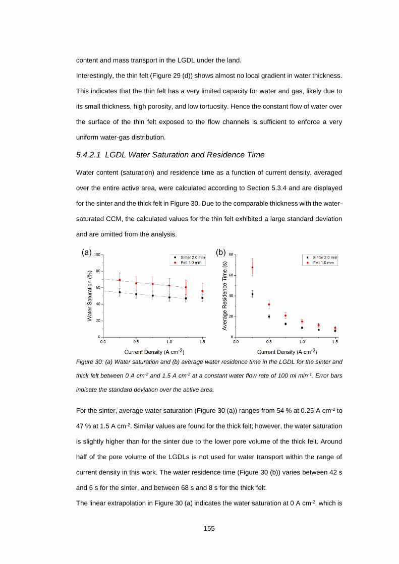
155
content and mass transport in the LGDL under the land.
Interestingly, the thin felt (Figure 29 (d)) shows almost no local gradient in water thickness.
This indicates that the thin felt has a very limited capacity for water and gas, likely due to
its small thickness, high porosity, and low tortuosity. Hence the constant flow of water over
the surface of the thin felt exposed to the flow channels is sufficient to enforce a very
uniform water-gas distribution.
5.4.2.1 LGDL Water Saturation and Residence Time
Water content (saturation) and residence time as a function of current density, averaged
over the entire active area, were calculated according to Section 5.3.4 and are displayed
for the sinter and the thick felt in Figure 30. Due to the comparable thickness with the water-
saturated CCM, the calculated values for the thin felt exhibited a large standard deviation
and are omitted from the analysis.
Figure 30: (a) Water saturation and (b) average water residence time in the LGDL for the sinter and
thick felt between 0 A cm-2 and 1.5 A cm-2 at a constant water flow rate of 100 ml min-1. Error bars
indicate the standard deviation over the active area.
For the sinter, average water saturation (Figure 30 (a)) ranges from 54 % at 0.25 A cm-2 to
47 % at 1.5 A cm-2. Similar values are found for the thick felt; however, the water saturation
is slightly higher than for the sinter due to the lower pore volume of the thick felt. Around
half of the pore volume of the LGDLs is not used for water transport within the range of
current density in this work. The water residence time (Figure 30 (b)) varies between 42 s
and 6 s for the sinter, and between 68 s and 8 s for the thick felt.
The linear extrapolation in Figure 30 (a) indicates the water saturation at 0 A cm-2, which is
156
56.0 % and 70.6 % for the sinter and felt, respectively. This illustrates that a significant
fraction of the LGDL is not filled with water, even without gas being produced due to
electrochemical activity. The XCT analysis in Section 5.4.1 showed that a fraction of the
LGDL pores are disconnected and can therefore not contribute to the transport of gas and
water. However, for the sinter and thick felt there was only a moderate amount of
disconnected porosity, which is not significant enough to explain the low values of water
saturation obtained even at 0 A cm-2. This leads to the conclusion that a number of pores,
which are connected to the rest of the pore network, are not, or insufficiently, reached by
water flow (stranded pores). This effect has been computationally predicted for fibrous
materials used in redox flow batteries and is affiliated with small variations in local porosity
[260].
Based on this characterization, it is likely that the performance of a PEMWE could be further
improved by tailoring the LGDL to avoid disconnected or stranded (‘dead’) pore space. This
could be achieved by reducing pore volume, which increases electrical and thermal
conductivity but does not affect the mass transport properties of the LGDL. Another
potential approach is to create materials in which the formation of new water pathways is
favored, so that sufficient mass transport can be guaranteed even at elevated current
density. The approach of combining neutron radiography and XCT is a promising technique
for the evaluation of new materials and LDGL architectures.
157
5.5 Conclusion
This work combines X-ray micro-computed tomography and neutron radiography to
investigate the link between LGDL microstructure and mass transport properties. Three
different LGDLs were examined (one sintered and two fibrous materials); the sinter was
found to have a porosity of ~30 %, while the thick and thin felt have porosities of 47 % and
77 %, respectively. Pore network models were created from the XCT datasets and used to
calculate the flux of water through individual throats of the LGDL. It was found that the flow
occurs predominantly through a small fraction of throats, supporting the idea of preferential
pathways through the LGDL.
Neutron radiography was employed for operando imaging of a PEMWE, varying the LGDL
material. Various differences between the three LGDLs were observed during the operation
of the PEMWE, with water thickness being clearly influenced by the thickness and porosity
of the LGDL. The imaging also revealed the structure of oxygen bubbles in the flow
channels, and locations with an increased gas fraction.
To further investigate the differences between LGDL materials, the water thickness under
the rib areas of the flow-fields was analysed. This offers the potential to observe the
spatially-resolved water content in the LGDL only.
The main findings from this analysis are:
Neutron radiography is a powerful tool to visualize the water-gas distribution in
PEMWE flow channels operando, enabling analysis of the link between flow-field
geometry and flow phenomena, facilitating the analysis and optimisation of
PEMWE architecture.
A decrease in water thickness with increasing current density was revealed for all
LGDLs, which is caused by the increased rate of gas production.
Significant inhomogeneity in water thickness was observed for the sinter and the
thick felt across the active area. This highlights the need for novel LGDL structures
or materials to avoid poor performance due to local mass transport limitations at
high current density.
Increased water thickness was found in areas that are likely to exhibit increased
158
flow velocity in the flow channels. This indicates a link between flow-field geometry
and mass transport in the LGDL which has not been previously reported in
literature.
By combining water thickness data obtained by neutron radiography and microstructural
information gained from XCT, water saturation and water residence time in the pores of the
LGDLs were calculated. It was revealed that around half of the pore volume is not utilized
for water transport and that this value varies only slightly with increasing current density.
Further, the water residence time in the LGDL was measured to range between 6 s and
68 s. Extrapolation to 0 A cm-2 shows that a significant fraction of pores remain dry, even
in the absence of electrochemical activity. This cannot be explained from the amount of
disconnected pores found in the XCT analysis and therefore implies the existence of
stranded pores. These pores are connected to the overall pore network, but no water flow
through them occurs due to small scale variations in porosity in the vicinity of these pores.
This indicates that further improvements on LGDL structure and materials need to be made
to increase pore utilization. The reduction of unused pore volume can potentially lead to
improved usage of active area and hence to an improvement in the efficiency of PEMWEs.
The above findings illustrate the excellent capabilities of neutron imaging as a diagnostic
tool for PEMWEs. The combination of neutron radiography and XCT yields deep insight
into the mass transport characteristics of LGDLs, which would not be possible by either of
these techniques alone. The findings give an indication of the shortcomings of the materials
most frequently used as LGDLs in PEMWEs and suggest pathways to novel structures that
could mitigate these issues.
However, methods such as neutron imaging and XCT are time-consuming and require
expensive equipment with limited access. Therefore, the following sections are dedicated
to establishing a set of new acoustic diagnostic tools, which in some cases can provide
rapid and low-cost alternatives to the imaging methods used so far.
159
6 Two-Phase Flow Diagnosis in PEMWE Flow Channels with Acoustic Emission

161
6.1 Overview
In this chapter, acoustic emission analysis is used as a low-cost, non-destructive, operando
diagnostic tool to provide information about the relative number and size of gas bubbles
generated locally within a PEMWE, providing effective characterization of the local flow
conditions. An optically transparent single-channel PEMWE is used to investigate the
relationship between the acoustic signals obtained and the two-phase flow conditions
inside the cell. The number of acoustic hits, their frequency, and average peak amplitude
is reported for several flow rates and current densities. Using high-speed imaging, the
average bubble number and size in the flow channels is compared to the acoustic signal.
Results show good correlation between the number of acoustic ‘hits’ and the number of
bubbles passing through the flow channel. The size of bubbles is also shown to affect the
average frequency of the hits. Consequently, the transition between bubbly and slug flow
regime can be identified by acoustic emission analysis, paving the way for a simple, low-
cost, non-destructive means of mapping flow inside PEMWEs.
Building on these results, acoustic emission is applied to a PEMWE with a parallel flow-
field, diagnosing a sudden drop in the number of acoustic hits, while hit duration, amplitude,
and energy increase significantly as the current density is increased from 0.5 A cm-2 to
1 A cm-2. It is found that the change in acoustic regime coincides with a significant
extension of the stagnant bubble region in the flow channels of the PEMWE, observed with
high-speed optical imaging. These results demonstrate that acoustic emission can be used
effectively as an operando diagnostic tool to monitor bubble formation (two-phase flow
conditions) in PEMWEs, facilitating rapid testing or prototyping, and contributing to
operational safety. Further, this establishes acoustic emission as an alternative method of
investigating processes in the flow channels to expensive and less accessible techniques
such as neutron imaging.
The results in this chapter form part of publications by the author in Journal of Power
Sources [218] and Frontiers in Energy [261].
162
6.2 Introduction
Understanding how various factors influence performance and durability of a PEMWE is
key to optimising cell design, component materials, and operating conditions. Various
diagnostic techniques have been applied to PEMWEs to gain greater insight into their
operation. These techniques range from computational methods [55,100,262] to avoid
costs of production and experimentation and low-cost, readily-available techniques which
only require access to a potentiostat, such as electrochemical impedance spectroscopy to
identify electrochemical losses in a system [43,118], to high-end experiments such as
neutron imaging used to visualize water content in the liquid-gas diffusion layer [88,89],
bubble dynamics, and flow regimes [85–87].
This chapter aims to deliver a simple low-cost diagnostic tool of two-phase flow in
operational PEMWEs without the need for any cell modification. High-speed flow
visualisation using a single-channel optical PEMWE is combined with local AE
measurements to correlate acoustic signals with flow characteristics with a view to
establishing a diagnostic tool for standard (unmodified) PEMWEs. AE is a low-cost, non-
destructive, operando diagnostic tool, detecting mechanical perturbations in a sample with
a sensor mounted to the external sample surface (Figure 31).
Two different PEMWE cell designs are used, each focused on investigating different flow
processes. A single-channel cell is used to show the effects of varying current density and
flow regimes on the AE signal, while the influence of stagnant gas bubbles in the flow
channels was investigated in a PEMWE cell with a parallel flow-field.
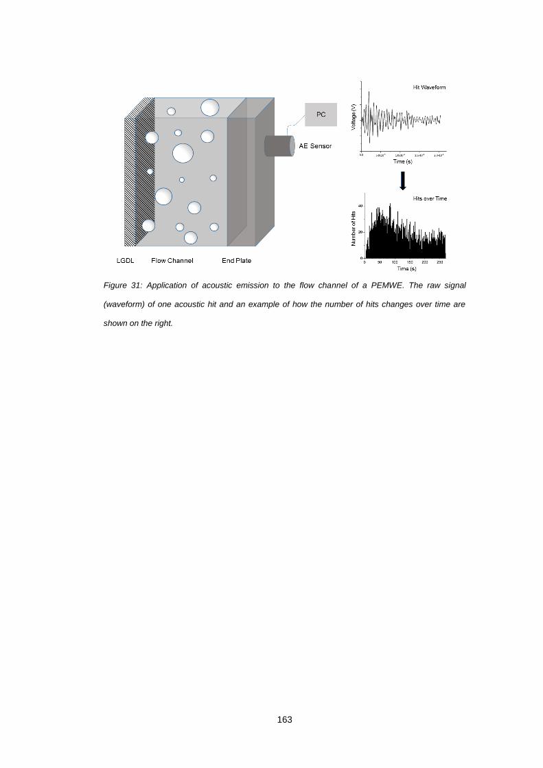
163
Figure 31: Application of acoustic emission to the flow channel of a PEMWE. The raw signal
(waveform) of one acoustic hit and an example of how the number of hits changes over time are
shown on the right.
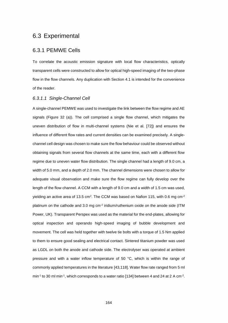
164
6.3 Experimental
6.3.1 PEMWE Cells
To correlate the acoustic emission signature with local flow characteristics, optically
transparent cells were constructed to allow for optical high-speed imaging of the two-phase
flow in the flow channels. Any duplication with Section 4.1 is intended for the convenience
of the reader.
6.3.1.1 Single-Channel Cell
A single-channel PEMWE was used to investigate the link between the flow regime and AE
signals (Figure 32 (a)). The cell comprised a single flow channel, which mitigates the
uneven distribution of flow in multi-channel systems (Nie et al. [72]) and ensures the
influence of different flow rates and current densities can be examined precisely. A single-
channel cell design was chosen to make sure the flow behaviour could be observed without
obtaining signals from several flow channels at the same time, each with a different flow
regime due to uneven water flow distribution. The single channel had a length of 9.0 cm, a
width of 5.0 mm, and a depth of 2.0 mm. The channel dimensions were chosen to allow for
adequate visual observation and make sure the flow regime can fully develop over the
length of the flow channel. A CCM with a length of 9.0 cm and a width of 1.5 cm was used,
yielding an active area of 13.5 cm2. The CCM was based on Nafion 115, with 0.6 mg cm-2
platinum on the cathode and 3.0 mg cm-2 iridium/ruthenium oxide on the anode side (ITM
Power, UK). Transparent Perspex was used as the material for the end-plates, allowing for
optical inspection and operando high-speed imaging of bubble development and
movement. The cell was held together with twelve tie bolts with a torque of 1.5 Nm applied
to them to ensure good sealing and electrical contact. Sintered titanium powder was used
as LGDL on both the anode and cathode side. The electrolyser was operated at ambient
pressure and with a water inflow temperature of 50 °C, which is within the range of
commonly applied temperatures in the literature [43,118]. Water flow rate ranged from 5 ml
min-1 to 30 ml min-1, which corresponds to a water ratio [134] between 4 and 24 at 2 A cm-2.
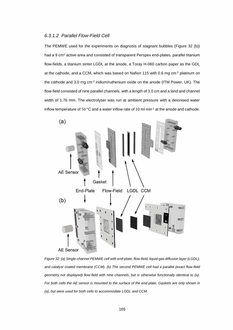
165
6.3.1.2 Parallel Flow-Field Cell
The PEMWE used for the experiments on diagnosis of stagnant bubbles (Figure 32 (b))
had a 9 cm2 active area and consisted of transparent Perspex end-plates, parallel titanium
flow-fields, a titanium sinter LGDL at the anode, a Toray H-060 carbon paper as the GDL
at the cathode, and a CCM, which was based on Nafion 115 with 0.6 mg cm-2 platinum on
the cathode and 3.0 mg cm-2 iridium/ruthenium oxide on the anode (ITM Power, UK). The
flow-field consisted of nine parallel channels, with a length of 3.0 cm and a land and channel
width of 1.76 mm. The electrolyser was run at ambient pressure with a deionised water
inflow temperature of 50 °C and a water inflow rate of 10 ml min-1 at the anode and cathode.
Figure 32: (a) Single-channel PEMWE cell with end-plate, flow-field, liquid-gas diffusion layer (LGDL),
and catalyst coated membrane (CCM). (b) The second PEMWE cell had a parallel (exact flow-field
geometry not displayed) flow-field with nine channels, but is otherwise functionally identical to (a).
For both cells the AE sensor is mounted to the surface of the end-plate. Gaskets are only shown in
(a), but were used for both cells to accommodate LGDL and CCM.
166
6.3.2 Electrochemical Testing
The electrochemical performance of the single-channel and the parallel flow-field cell can
be seen in Figure 33, with both cells showing typical polarisation behaviour and the voltage
within the range of typical values reported in the literature [31,43,59,120].
Figure 33: Electrochemical performance of (a) the single-channel, and (b) the parallel flow-field
PEMWE between 0 A cm-2 and 2 A cm-2.
A potentiostat (Gamry Reference 3000 Galvanostat/Potentiostat with a Gamry 30k Booster;
Gamry Instruments, USA) was used for electrochemical testing with the current density
ranging between 0 A cm-2 and 2 A cm-2.
6.3.3 Acoustic Emission
The acoustic emission of the PEMWEs was monitored using a piezoelectric sensor (S9208;
Mistras NDT, UK). The signal was filtered and pre-amplified by 26 dB and a digital node
extracted an acoustic hit from the continuous signal whenever the noise threshold of 37 dB
was exceeded. For each data point, acoustic data was recorded over the course of 1 minute
167
during galvanostatic operation of the PEMWE cell. The AE sensor was mounted on the
anode side, with two different locations investigated. Acoustic signals arising from the
cathode are a potential source of error; however, it is unlikely that a significant magnitude
of acoustic signal can pass through the various acoustic impedances from the cathode to
the anode side. This is especially significant for the interface between anode LGDL and
flow channel, which would need to be passed by any signal from the cathode side. As this
is a solid/liquid interface, it is likely that up to 90 % of the signal is reflected [247].
6.3.3.1 Sensor Positioning
For the single-channel PEMWE, two separate points of interest (sensor locations) were
chosen. The lower point of interest was located 1.5 cm from the start of the flow channel
near the inlet; the upper location 1.5 cm from the top of the channel near the outlet. These
two distinct locations were chosen so as to represent markedly different flow regimes as
typically 400 % more gas has to pass through the upper location. For the parallel flow-field
cell, the sensor was placed in the centre of the flow-field.
Due to the nature of sound transmission, no clear area can be defined within which acoustic
data is collected. Whether a mechanical perturbation is detected by the sensor is contingent
on the location and intensity of the perturbation, with the intensity necessary for detection
increasing with the distance between acoustic source and sensor. Therefore, detection of
bubbles is increasingly likely as they are located closer to the sensor.
6.3.4 Acoustic Emission Post-Processing
Data collection and analysis was performed using the commercial software AEWin
(Physical Acoustics, USA). The number of acoustic hits per unit time (hit rate 𝐻), the
corresponding average frequency of hits 𝑓, and their average amplitude 𝐴 were recorded
for the single-cell PEMWE. For the parallel flow-field PEMWE, the hit rate, the average hit
amplitude, the averaged time from exceeding the threshold until falling back below it
(average hit duration 𝐷) and the average hit energy 𝐸 were analysed. An acoustic hit is
registered whenever the amplitude of the acoustic signal exceeds a certain predefined
threshold; it ends when the signal has permanently damped back below the threshold.
When the signal associated with an acoustic hit is analysed by fast Fourier transform (FFT)

168
or similar techniques, a characteristic peak frequency is obtained. By averaging the peak
frequency of all hits occurring within one sampling period, the average peak frequency 𝑓 is
obtained. This is the frequency of the voltage-time profile of a specific AE hit averaged over
all hits; it is not the frequency with which hits occur over time. Various studies have
established that bubble oscillations cause pressure impulses at a frequency specific to
bubble size, which can be picked up by AE [193,263–265]. The necessary equations to
analyse the frequency information gained through FFT can be found in Section 4.4.2.1.
6.3.5 High-Speed Imaging
A high-speed camera (Photron FASTCAM SA1) was used for imaging of the flow
channel(s). Images were taken at 2000 frames per second and a resolution of 1024×1024
pixels over the course of 5.46 s (maximum available acquisition time at this frame rate) for
each set of experimental conditions. A temporal resolution of 2000 frames per second was
chosen to ensure no feature of the flow was missed, and the evolution of flow regime along
the channel could be observed with high temporal detail. This resulted in 10920 images for
each set of conditions, which offers a large set of data for quantitative analysis. For the
single-channel cell, quantitative analysis of the image sets was performed to calculate the
number and size of captured bubbles (see Section 4.2.1).
The images of the single-channel cell used for quantitative analysis were high-resolution
images of the region where the AE sensor was placed, taken with a Tokina MACRO 100
F2.8 D lens (spatial resolution 50 µm), whereas the whole length of the flow channel was
captured with a Sigma 1:2.8 DG HSM lens (spatial resolution 300 µm). For the parallel flow-
field cell, the Tokina MACRO 100 F2.8 D lens was used as well, but the obtained images
were not analysed quantitatively.
6.3.6 Image Post-Processing
MATLAB (MathWorks) was used to perform all necessary post-processing steps. As
outlined in Section 4.2.1, images were thresholded, filtered, circular structures in the
images were identified, and finally, overlapping circles were removed (only retaining the
largest overlapping circle. Size D and number N of bubbles were then averaged for all
images within one set of conditions. The lower detection limit for this algorithm is a diameter
169
of 5 pixels, equalling 125 µm. The process is limited to circular bubbles, which means that
in the case of elliptic slug bubbles only the length of the minor axis of the bubble is
registered. To reduce computation time, only every 10th image was used for data analysis.
The resulting number of more than 1000 analysed images is sufficient for representative
analysis. To make sure the algorithm produces trustworthy results, bubble size and number
were also determined manually over the current density range for a water flow rate of 5 ml
min-1, by counting and measuring gas bubbles in seven randomly selected images for each
current density. In the case of non-spherical gas bubbles, the size of the bubble was taken
as the length of the minor axis.
170
6.4 Results
6.4.1 Flow Regime Diagnosis in a Single-Channel PEMWE
The typical characteristics of acoustic emission in the single-channel cell are shown in
Figure 34 for different flow rates over a range of current density at both sensor locations.
For the upper location, the number of hits (Figure 34 (a)) rapidly increases initially and
reaches a maximum at around 0.5 A cm-2. The number of hits then decreases and reaches
a plateau at approximately 1.5 A cm-2. For low current densities (< 0.5 A cm-2), the water
flow rate has a negligible influence, whereas above this value the number of hits is a clear
function of flow rate, reaching values of 5 hits per second at 5 ml min-1 and 12 hits per
second at 30 ml min-1. This provides a correlation between flow processes in the PEMWE
and its acoustic emission. In contrast, at the lower channel location the peak is less
pronounced (Figure 34(d)), with the peak value at different current densities ranging from
0.5 A cm-2 to 0.8 A cm-2, and a much less prominent decrease in the number of hits at
higher current densities.
Figure 34 (b) and (e) illustrate the average peak frequency of AE hits as a function of current
density. As discussed in Section 4.4.2.1, the frequency of bubble oscillation is linked to
bubble size. Hence, the results from Figure 34 (b) and (e) imply a constant increase in
bubble size at both the upper and lower locations, as the mass of oxygen produced
increases with current density. However, the frequency decreases by 14.5 kHz (A cm-2)-1
for the upper location, but only 9 kHz (A cm-2)-1 for the lower location.
Again, this is in line with expectation as for the upper location approximately 400% more
gas is passing through the flow channel and therefore relative changes in bubble size
between low and high current density are expected to be more pronounced.
At the same time, it can be seen from Figure 34 (c) and (f) that the average amplitude of
AE hits is relatively independent of current density for both locations, as the value of 𝐴 is
constant as a function of current density. If the number of bubbles is expected to change
when varying current density, this would lead to a changing amplitude of the AE signal (see
Section 4.4.2.1) if it is assumed that the acoustic hits are emitted as a consequence of
simultaneous oscillations. Hence, the invariance of amplitude implies that the signal does
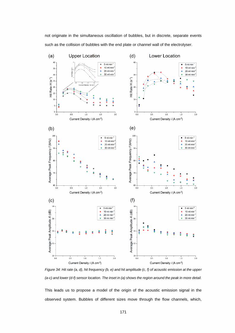
171
not originate in the simultaneous oscillation of bubbles, but in discrete, separate events
such as the collision of bubbles with the end plate or channel wall of the electrolyser.
Figure 34: Hit rate (a, d), hit frequency (b, e) and hit amplitude (c, f) of acoustic emission at the upper
(a-c) and lower (d-f) sensor location. The inset in (a) shows the region around the peak in more detail.
This leads us to propose a model of the origin of the acoustic emission signal in the
observed system. Bubbles of different sizes move through the flow channels, which,
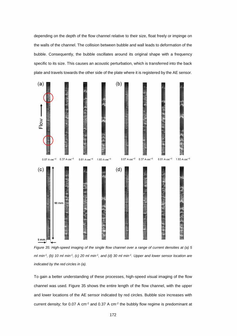
172
depending on the depth of the flow channel relative to their size, float freely or impinge on
the walls of the channel. The collision between bubble and wall leads to deformation of the
bubble. Consequently, the bubble oscillates around its original shape with a frequency
specific to its size. This causes an acoustic perturbation, which is transferred into the back
plate and travels towards the other side of the plate where it is registered by the AE sensor.
Figure 35: High-speed imaging of the single flow channel over a range of current densities at (a) 5
ml min-1, (b) 10 ml min-1, (c) 20 ml min-1, and (d) 30 ml min-1. Upper and lower sensor location are
indicated by the red circles in (a).
To gain a better understanding of these processes, high-speed visual imaging of the flow
channel was used. Figure 35 shows the entire length of the flow channel, with the upper
and lower locations of the AE sensor indicated by red circles. Bubble size increases with
current density; for 0.07 A cm-2 and 0.37 A cm-2 the bubbly flow regime is predominant at
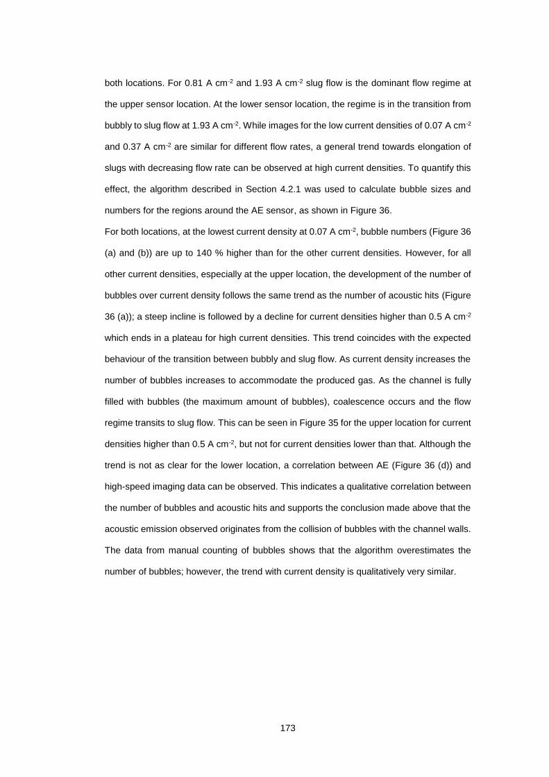
173
both locations. For 0.81 A cm-2 and 1.93 A cm-2 slug flow is the dominant flow regime at
the upper sensor location. At the lower sensor location, the regime is in the transition from
bubbly to slug flow at 1.93 A cm-2. While images for the low current densities of 0.07 A cm-2
and 0.37 A cm-2 are similar for different flow rates, a general trend towards elongation of
slugs with decreasing flow rate can be observed at high current densities. To quantify this
effect, the algorithm described in Section 4.2.1 was used to calculate bubble sizes and
numbers for the regions around the AE sensor, as shown in Figure 36.
For both locations, at the lowest current density at 0.07 A cm-2, bubble numbers (Figure 36
(a) and (b)) are up to 140 % higher than for the other current densities. However, for all
other current densities, especially at the upper location, the development of the number of
bubbles over current density follows the same trend as the number of acoustic hits (Figure
36 (a)); a steep incline is followed by a decline for current densities higher than 0.5 A cm-2
which ends in a plateau for high current densities. This trend coincides with the expected
behaviour of the transition between bubbly and slug flow. As current density increases the
number of bubbles increases to accommodate the produced gas. As the channel is fully
filled with bubbles (the maximum amount of bubbles), coalescence occurs and the flow
regime transits to slug flow. This can be seen in Figure 35 for the upper location for current
densities higher than 0.5 A cm-2, but not for current densities lower than that. Although the
trend is not as clear for the lower location, a correlation between AE (Figure 36 (d)) and
high-speed imaging data can be observed. This indicates a qualitative correlation between
the number of bubbles and acoustic hits and supports the conclusion made above that the
acoustic emission observed originates from the collision of bubbles with the channel walls.
The data from manual counting of bubbles shows that the algorithm overestimates the
number of bubbles; however, the trend with current density is qualitatively very similar.
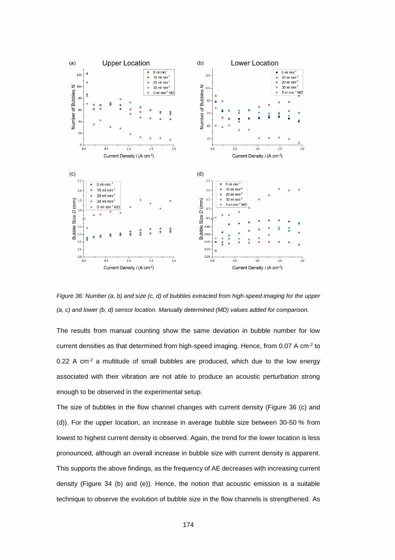
174
Figure 36: Number (a, b) and size (c, d) of bubbles extracted from high-speed imaging for the upper
(a, c) and lower (b, d) sensor location. Manually determined (MD) values added for comparison.
The results from manual counting show the same deviation in bubble number for low
current densities as that determined from high-speed imaging. Hence, from 0.07 A cm-2 to
0.22 A cm-2 a multitude of small bubbles are produced, which due to the low energy
associated with their vibration are not able to produce an acoustic perturbation strong
enough to be observed in the experimental setup.
The size of bubbles in the flow channel changes with current density (Figure 36 (c) and
(d)). For the upper location, an increase in average bubble size between 30-50 % from
lowest to highest current density is observed. Again, the trend for the lower location is less
pronounced, although an overall increase in bubble size with current density is apparent.
This supports the above findings, as the frequency of AE decreases with increasing current
density (Figure 34 (b) and (e)). Hence, the notion that acoustic emission is a suitable
technique to observe the evolution of bubble size in the flow channels is strengthened. As
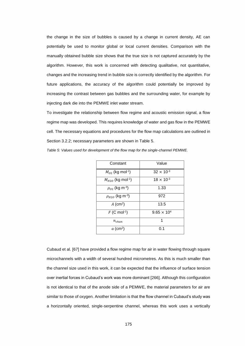
175
the change in the size of bubbles is caused by a change in current density, AE can
potentially be used to monitor global or local current densities. Comparison with the
manually obtained bubble size shows that the true size is not captured accurately by the
algorithm. However, this work is concerned with detecting qualitative, not quantitative,
changes and the increasing trend in bubble size is correctly identified by the algorithm. For
future applications, the accuracy of the algorithm could potentially be improved by
increasing the contrast between gas bubbles and the surrounding water, for example by
injecting dark die into the PEMWE inlet water stream.
To investigate the relationship between flow regime and acoustic emission signal, a flow
regime map was developed. This requires knowledge of water and gas flow in the PEMWE
cell. The necessary equations and procedures for the flow map calculations are outlined in
Section 3.2.2; necessary parameters are shown in Table 5.
Table 5: Values used for development of the flow map for the single-channel PEMWE.
Constant Value
𝑀𝑂2 (kg mol-1) 32 × 10-3
𝑀𝐻2𝑂 (kg mol-1) 18 × 10-3
𝜌𝑂2 (kg m-3) 1.33
𝜌𝐻2𝑂 (kg m-3) 972
𝐴 (cm2) 13.5
𝐹 (C mol-1) 9.65 × 10⁴
𝑛𝑐ℎ𝑎𝑛 1
𝑎 (cm2) 0.1
Cubaud et al. [67] have provided a flow regime map for air in water flowing through square
microchannels with a width of several hundred micrometres. As this is much smaller than
the channel size used in this work, it can be expected that the influence of surface tension
over inertial forces in Cubaud’s work was more dominant [266]. Although this configuration
is not identical to that of the anode side of a PEMWE, the material parameters for air are
similar to those of oxygen. Another limitation is that the flow channel in Cubaud’s study was
a horizontally oriented, single-serpentine channel, whereas this work uses a vertically
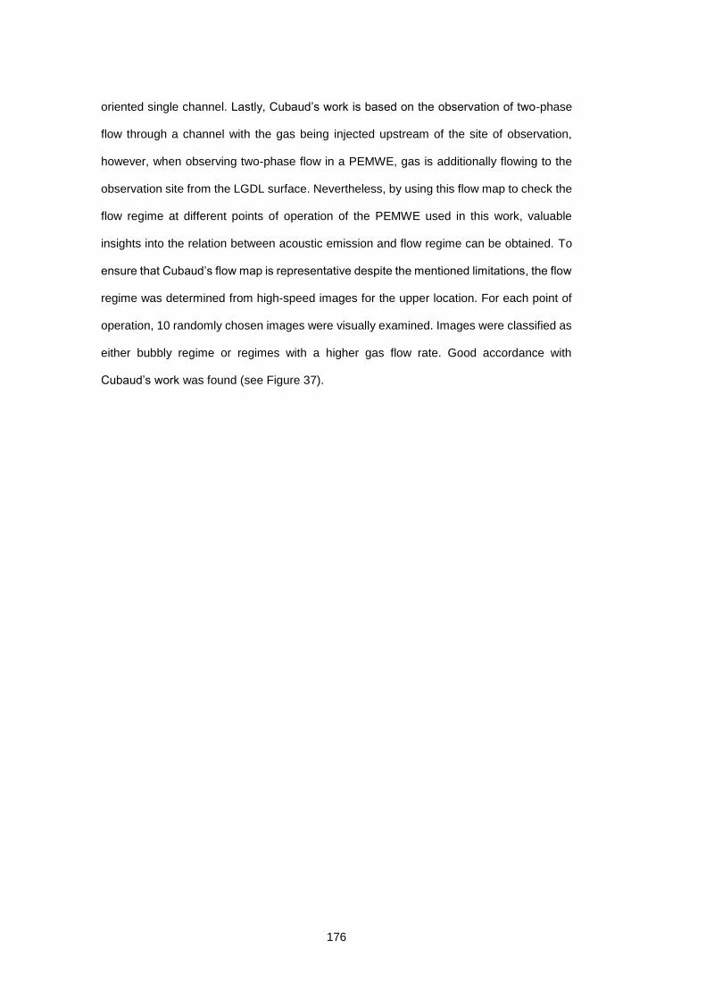
176
oriented single channel. Lastly, Cubaud’s work is based on the observation of two-phase
flow through a channel with the gas being injected upstream of the site of observation,
however, when observing two-phase flow in a PEMWE, gas is additionally flowing to the
observation site from the LGDL surface. Nevertheless, by using this flow map to check the
flow regime at different points of operation of the PEMWE used in this work, valuable
insights into the relation between acoustic emission and flow regime can be obtained. To
ensure that Cubaud’s flow map is representative despite the mentioned limitations, the flow
regime was determined from high-speed images for the upper location. For each point of
operation, 10 randomly chosen images were visually examined. Images were classified as
either bubbly regime or regimes with a higher gas flow rate. Good accordance with
Cubaud’s work was found (see Figure 37).
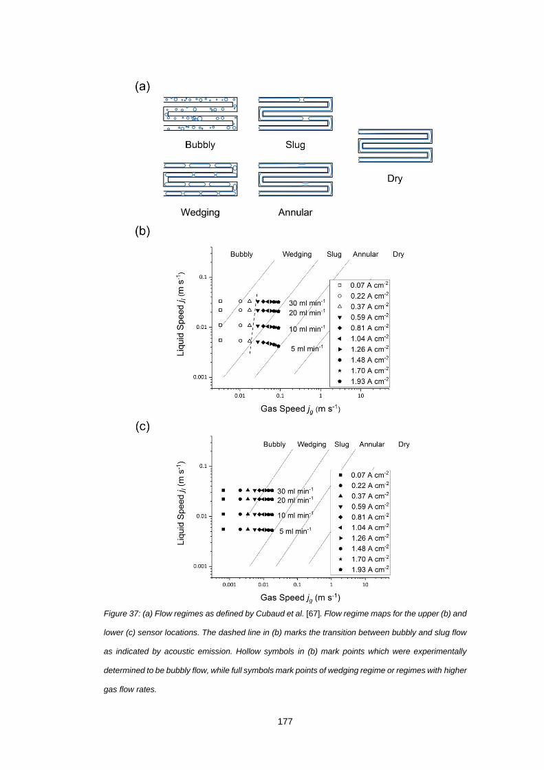
177
Figure 37: (a) Flow regimes as defined by Cubaud et al. [67]. Flow regime maps for the upper (b) and
lower (c) sensor locations. The dashed line in (b) marks the transition between bubbly and slug flow
as indicated by acoustic emission. Hollow symbols in (b) mark points which were experimentally
determined to be bubbly flow, while full symbols mark points of wedging regime or regimes with higher
gas flow rates.
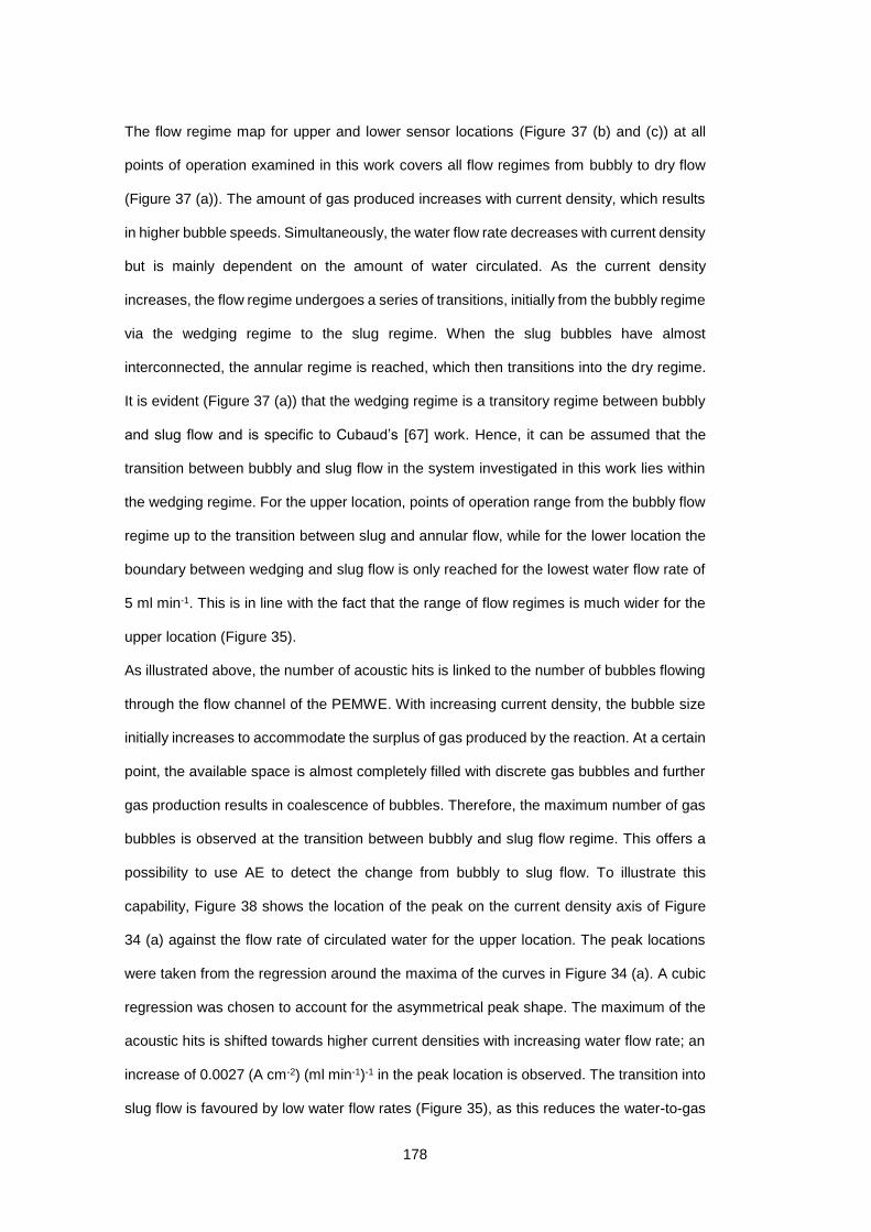
178
The flow regime map for upper and lower sensor locations (Figure 37 (b) and (c)) at all
points of operation examined in this work covers all flow regimes from bubbly to dry flow
(Figure 37 (a)). The amount of gas produced increases with current density, which results
in higher bubble speeds. Simultaneously, the water flow rate decreases with current density
but is mainly dependent on the amount of water circulated. As the current density
increases, the flow regime undergoes a series of transitions, initially from the bubbly regime
via the wedging regime to the slug regime. When the slug bubbles have almost
interconnected, the annular regime is reached, which then transitions into the dry regime.
It is evident (Figure 37 (a)) that the wedging regime is a transitory regime between bubbly
and slug flow and is specific to Cubaud’s [67] work. Hence, it can be assumed that the
transition between bubbly and slug flow in the system investigated in this work lies within
the wedging regime. For the upper location, points of operation range from the bubbly flow
regime up to the transition between slug and annular flow, while for the lower location the
boundary between wedging and slug flow is only reached for the lowest water flow rate of
5 ml min-1. This is in line with the fact that the range of flow regimes is much wider for the
upper location (Figure 35).
As illustrated above, the number of acoustic hits is linked to the number of bubbles flowing
through the flow channel of the PEMWE. With increasing current density, the bubble size
initially increases to accommodate the surplus of gas produced by the reaction. At a certain
point, the available space is almost completely filled with discrete gas bubbles and further
gas production results in coalescence of bubbles. Therefore, the maximum number of gas
bubbles is observed at the transition between bubbly and slug flow regime. This offers a
possibility to use AE to detect the change from bubbly to slug flow. To illustrate this
capability, Figure 38 shows the location of the peak on the current density axis of Figure
34 (a) against the flow rate of circulated water for the upper location. The peak locations
were taken from the regression around the maxima of the curves in Figure 34 (a). A cubic
regression was chosen to account for the asymmetrical peak shape. The maximum of the
acoustic hits is shifted towards higher current densities with increasing water flow rate; an
increase of 0.0027 (A cm-2) (ml min-1)-1 in the peak location is observed. The transition into
slug flow is favoured by low water flow rates (Figure 35), as this reduces the water-to-gas
179
ratio.
To further illustrate how acoustic emission can diagnose the regime within the flow
channels of a PEMWE, the peak locations from Figure 38 were connected by a dashed line
in Figure 37 (b). This line represents the transition between bubbly and slug flow for the
upper sensor location, as determined from AE. For the range of water flow rates
investigated in this work the predicted change to slug flow falls within the wedging regime,
which is a transitory regime between bubbly and slug flow. Furthermore, the regime border
as determined by AE corresponds to information gathered from high-speed imaging. The
gradient of the regime boundary is different from that observed in Cubaud’s flow map;
however, this is not surprising as the examined systems are not identical. The way in which
changes to the experimental system can affect the shape and location of regime
boundaries can be seen by comparing flow regime maps of different authors for similar
systems [65,67].
Figure 38: Current density at which the maximum number of acoustic hits was registered as a function
of water flow rate, which indicates the transition from bubbly to slug flow.
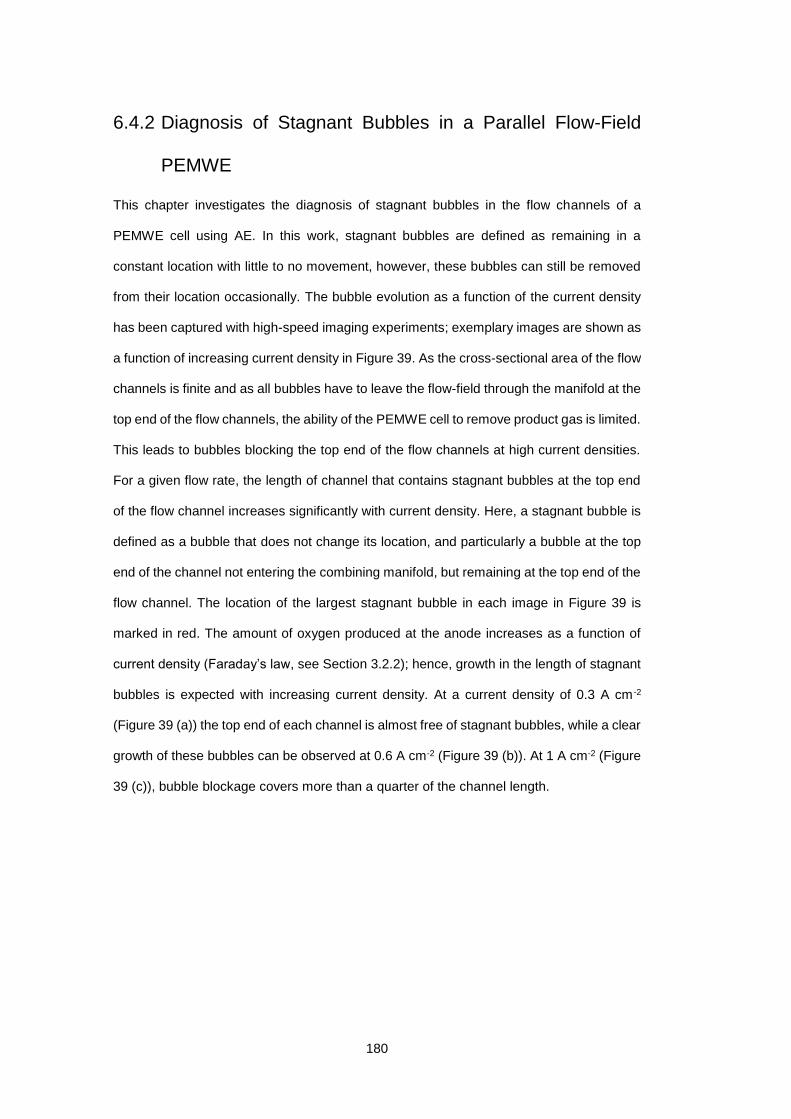
180
6.4.2 Diagnosis of Stagnant Bubbles in a Parallel Flow-Field
PEMWE
This chapter investigates the diagnosis of stagnant bubbles in the flow channels of a
PEMWE cell using AE. In this work, stagnant bubbles are defined as remaining in a
constant location with little to no movement, however, these bubbles can still be removed
from their location occasionally. The bubble evolution as a function of the current density
has been captured with high-speed imaging experiments; exemplary images are shown as
a function of increasing current density in Figure 39. As the cross-sectional area of the flow
channels is finite and as all bubbles have to leave the flow-field through the manifold at the
top end of the flow channels, the ability of the PEMWE cell to remove product gas is limited.
This leads to bubbles blocking the top end of the flow channels at high current densities.
For a given flow rate, the length of channel that contains stagnant bubbles at the top end
of the flow channel increases significantly with current density. Here, a stagnant bubble is
defined as a bubble that does not change its location, and particularly a bubble at the top
end of the channel not entering the combining manifold, but remaining at the top end of the
flow channel. The location of the largest stagnant bubble in each image in Figure 39 is
marked in red. The amount of oxygen produced at the anode increases as a function of
current density (Faraday’s law, see Section 3.2.2); hence, growth in the length of stagnant
bubbles is expected with increasing current density. At a current density of 0.3 A cm -2
(Figure 39 (a)) the top end of each channel is almost free of stagnant bubbles, while a clear
growth of these bubbles can be observed at 0.6 A cm-2 (Figure 39 (b)). At 1 A cm-2 (Figure
39 (c)), bubble blockage covers more than a quarter of the channel length.
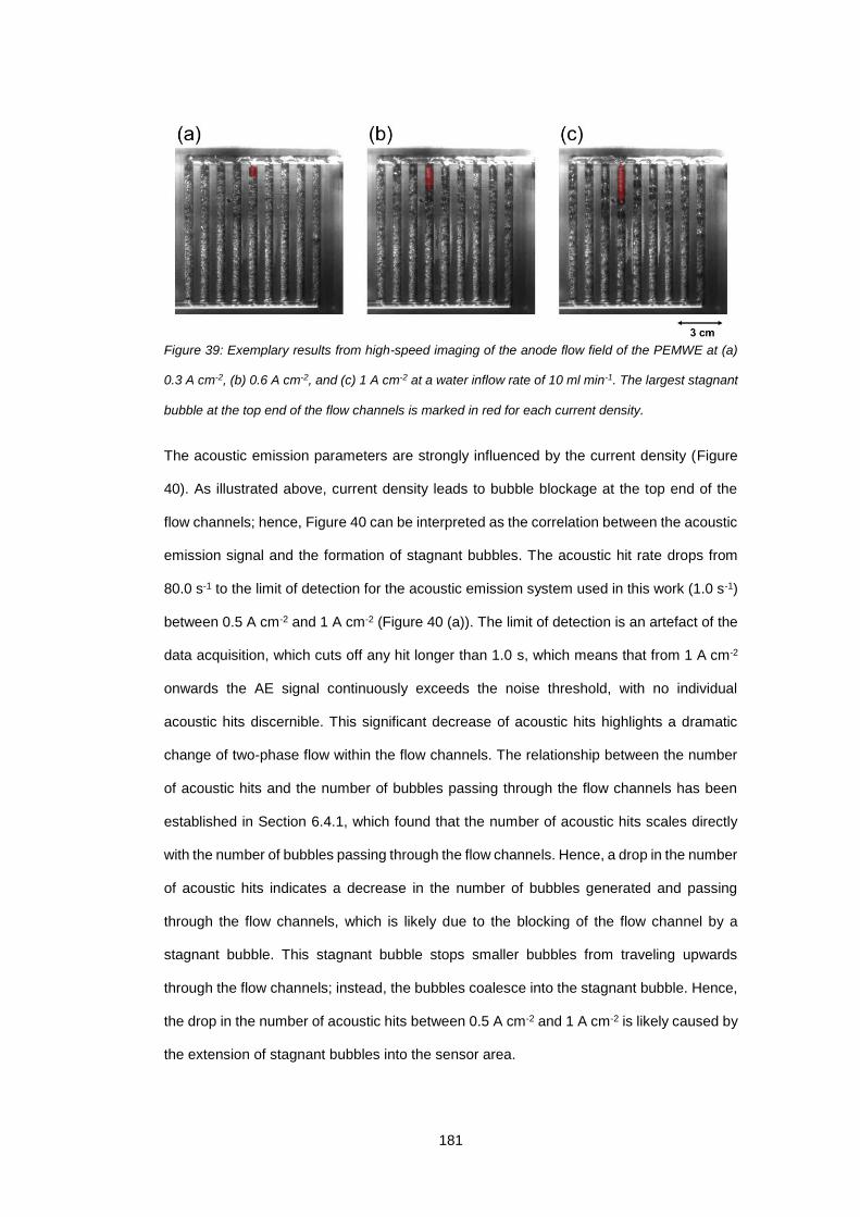
181
Figure 39: Exemplary results from high-speed imaging of the anode flow field of the PEMWE at (a)
0.3 A cm-2, (b) 0.6 A cm-2, and (c) 1 A cm-2 at a water inflow rate of 10 ml min-1. The largest stagnant
bubble at the top end of the flow channels is marked in red for each current density.
The acoustic emission parameters are strongly influenced by the current density (Figure
40). As illustrated above, current density leads to bubble blockage at the top end of the
flow channels; hence, Figure 40 can be interpreted as the correlation between the acoustic
emission signal and the formation of stagnant bubbles. The acoustic hit rate drops from
80.0 s-1 to the limit of detection for the acoustic emission system used in this work (1.0 s-1)
between 0.5 A cm-2 and 1 A cm-2 (Figure 40 (a)). The limit of detection is an artefact of the
data acquisition, which cuts off any hit longer than 1.0 s, which means that from 1 A cm-2
onwards the AE signal continuously exceeds the noise threshold, with no individual
acoustic hits discernible. This significant decrease of acoustic hits highlights a dramatic
change of two-phase flow within the flow channels. The relationship between the number
of acoustic hits and the number of bubbles passing through the flow channels has been
established in Section 6.4.1, which found that the number of acoustic hits scales directly
with the number of bubbles passing through the flow channels. Hence, a drop in the number
of acoustic hits indicates a decrease in the number of bubbles generated and passing
through the flow channels, which is likely due to the blocking of the flow channel by a
stagnant bubble. This stagnant bubble stops smaller bubbles from traveling upwards
through the flow channels; instead, the bubbles coalesce into the stagnant bubble. Hence,
the drop in the number of acoustic hits between 0.5 A cm-2 and 1 A cm-2 is likely caused by
the extension of stagnant bubbles into the sensor area.
182
Figure 40: Acoustic emission parameters as a function of current density for a water inflow rate of
10 ml min-1. Acoustic hit rate (a), average hit amplitude (b), average hit duration (c), and average hit
energy (d) are shown.
Further, the average hit amplitude (Figure 40 (b)) increases steeply by around 50 %
between 0.5 A cm-2 and 1 A cm-2, the same range within which the hit rate drops. The
average hit duration increases from less than 0.1 ms to the cut off value of 1.0 s mentioned
above (Figure 40 (c)). For current densities above 1 A cm-2, a constant signal is detected,
indicating permanent contact between a bubble and the end-plate. Finally, an increase in
hit duration and amplitude causes an increase in acoustic energy (Figure 40 (d)). All these
changes occur in a step-like manner between 0.5 A cm-2 and 1 A cm-2.
The decreasing number of hits, while hit amplitude and contact time between bubble and
end-plate increase, all suggest that the signal change is caused by the extension of the

183
stagnant bubble region towards the sensor location in the current density range between
0.5 A cm-2 and 1 A cm-2 (Figure 40). This is supported by the extension of the stagnant
bubble region, observed via high-speed imaging (Figure 39), a major part of which occurs
between 0.6 A cm-2 and 1 A cm-2.
184
6.5 Conclusion
This chapter successfully demonstrated the potential of acoustic emission as a low-cost
diagnostic tool for PEMWEs; in particular to study two-phase flow within the flow channels
during gas formation. Two studies on different PEMWE cells showed the capability of AE
to diagnose the flow regime and stagnant bubbles in the flow channels.
A close link between bubble size and number within the flow channel of a PEMWE and the
AE measured on the surface of the end-plates has been established. Two locations along
the single flow channel of a PEMWE have been investigated via AE measurements and
high-speed imaging. For the upper location, AE measurements showed that the number of
acoustic hits reaches a maximum around 0.5 A cm-2 and decreases to a plateau at higher
current densities. The average frequency of these hits decreases with current density,
which can be attributed to an increase in average bubble size. High-speed imaging at the
upper location is consistent with the acoustic emission results. The number of bubbles
detected follows the same trend as the number of acoustic hits with current density. This
implies that AE can monitor relative changes in the number of bubbles flowing through an
electrolyser and therefore can detect the change between bubbly and slug flow regime.
Image analysis also showed a trend towards increasing bubble size at higher current
densities, which supports the frequency data from acoustic emission; hence, AE can be
used to detect changes in bubble size in a PEMWE. Similar trends were observed for the
lower location; however, not as pronounced as for the upper location. This is consistent
with smaller amounts of gas passing by the lower location, which causes the relative
changes in bubble number and size to be less significant.
To further strengthen the link between acoustic emission and flow regime diagnosis, a flow
map was invoked. The states of operation in the PEMWE for this study covered the range
from bubbly flow to the onset of the annular regime. By analysing the current density at
which the number of acoustic hits reaches its maximum, a regime boundary between
bubbly and slug flow for the flow system used in this work was found. This regime boundary
lies within the wedging regime, as defined by Cubaud et al. [67], which is a transitory regime
between bubbly and slug flow. This supports the idea that the maximum of acoustic hits is

185
found at the transition between the bubbly and the slug regime and hence implies that
acoustic emission can be used to identify this regime change. As the number and size of
bubbles in a PEMWE are consequences of local and global current density, AE can offer
novel insight into the flow characteristics of the system and, potentially, local non-uniformity
in the distribution of current density.
In a separate study, acoustic emission has been demonstrated as a useful technique for
operando diagnosis of bubble blockage in a single-cell PEMWE. High-speed imaging of an
optically-transparent PEMWE cell with a parallel flow-field was used to visualize the bubble
movement in the flow channels. The length of the part of the flow channel containing
stagnant bubbles was found to increase with current density, eventually reaching the
location of the acoustic emission sensor. With increasing flow channel blockage, a dramatic
change in acoustic activity was observed. The acoustic hit rate dropped from 80.0 s-1 to
1.0 s-1, average hit amplitude increased from 32 dB to 50 dB, average hit duration from 0.1
ms to 1.0 s and average hit energy from 0.004 aJ to 3400 aJ. These changes occurred
abruptly between 0.5 A cm-2 and 1 A cm-2, which coincides with a significant extension of
the stagnant bubble region in the flow channels. This leads us to conclude that the change
in acoustic activity is caused by the flow regime in the channels changing from two-phase
flow to stagnant bubbles. The accumulation of gas in the flow channels occurs when gas
production exceeds the capacity of the system for gas removal, which can affect the water
distribution in the PEMWE. Further, as the accumulation of gas in the flow channels is
strongly affected by the flow-field geometry, the results in this work also demonstrate the
potential of using AE to screen different flow-field geometries for gas blockage and draw
conclusions on how to optimise flow-field designs.
The use of this operando diagnostic tool has successfully been applied to PEMWEs, but
could be extended to other applications. The accumulation of gas within a system or plant
can cause inefficiencies or pose a hazard in many areas of chemical production and
transport. Moreover, it has been shown that the change of two-phase flow regime
influences the pressure drop [67,267]. Hence, the technique presented in this chapter could
be deployed to screen various flow-field configurations or monitor safe limits of operation,
replacing less cost-effective or accessible diagnostic tools such as neutron or X-ray
186
imaging [83,88,90].
However, due to the strong acoustic signal obtained from the flow channels, it was not
possible to investigate LGDL mass transport processes using AE. Further, the use of an
individual sensor requires the repetition of experiments with different sensor locations to
obtain spatially resolved information. In response to these shortcomings, acoustic time-of-
flight imaging will be introduced in the following section as a diagnostic tool providing
spatially-resolved data on the water-gas distribution in the flow channels as well as the
LGDL.
187
7 Acoustic Time-of-Flight Imaging of PEMWEs to Probe Internal Structure and Flow Characteristics

189
7.1 Overview
In this chapter, acoustic time-of-flight (AToF) imaging has been demonstrated as a low-
cost, rapid, non-destructive, operando tool to characterize processes in the flow channels
and LGDL of a PEMWE. An array of 64 piezoelectric sensors was used, with all sensors
emitting input pulses and detecting the acoustic wave reflected by the sample (pulse-echo
mode). The shape and intensity of this reflected waveform depends on the ratio of reflection
and transmission at phase interfaces and is strongly affected by resonant scattering of
acoustic waves by gas bubbles. This AToF imaging technique was deployed to produce
reflection intensity maps of the anode flow-field and LGDL; by measuring the AToF
response for current densities ranging from 0 A cm-2 to 2 A cm-2, a close correlation was
found between the acoustic attenuation in the flow-field and the production and removal of
oxygen gas through the flow channels. Furthermore, a close link between the AToF
response and water thickness in the LGDL was demonstrated, as supported by literature
data. The application of AToF imaging has been established as a novel technique of
investigating PEMWE operation and as an alternative to more complex imaging techniques
such as neutron imaging. The work in this chapter has been published in International
Journal of Hydrogen Energy [268].
190
7.2 Introduction
The widespread industrial use of PEMWEs for hydrogen production and grid stabilization
will be accelerated through advances in the performance and cost of the technology. One
of the most effective ways of improving such technology is through the establishment and
use of a robust set of metrology tools to screen the effect of design modification, support
optimization of operational parameters and facilitate low-cost maintenance and repair.
Traditional electrochemical testing methods, including the interpretation of polarization
curves and electrochemical impedance spectroscopy, are valuable diagnostic techniques,
but do not offer the same level of spatially resolved information as modern imaging
technologies. X-ray computed tomography [153,156,170,172], neutron imaging [85,88–90]
or optical imaging [43,44,73,81] have been used to visualise internal operational processes
such as the two-phase flow in the flow channels, the microstructure of the liquid-gas
diffusion layer (LGDL), water-gas dynamics in the LGDL, or the particle structure of the
catalyst layer. However, these techniques are often expensive and may require adaptations
of the PEMWE cell to facilitate measurement.
Acoustic diagnostic techniques can overcome many of these disadvantages and promise
low-cost, fast, and non-destructive operando analysis of PEMWEs and other
electrochemical energy storage and conversion devices. AToF is an acoustic technique
wherein samples are actively probed with ultrasound waves; the transmitted or reflected
response signal is recorded as a function of time-of-flight (ToF) through the sample. The
intensity of a reflection signal depends on how strongly the input signal has been attenuated
by the sample. Acoustic attenuation occurs at an interface between two different phases
due to reflection or resonant scattering, for example from a gas bubble or group of bubbles
(Figure 41). At each interface, a portion of the incoming signal is reflected, while the
remaining signal is transmitted into the next domain. When an acoustic signal interacts with
a bubble interface, it is not only partially reflected, but can also be resonantly scattered if
the signal frequency is close to the resonant frequency of the bubble. In this case, the
signal is scattered in all directions, causing a very high acoustic attenuation of the input
signal. A more detailed discussion of acoustic attenuation mechanisms is found in
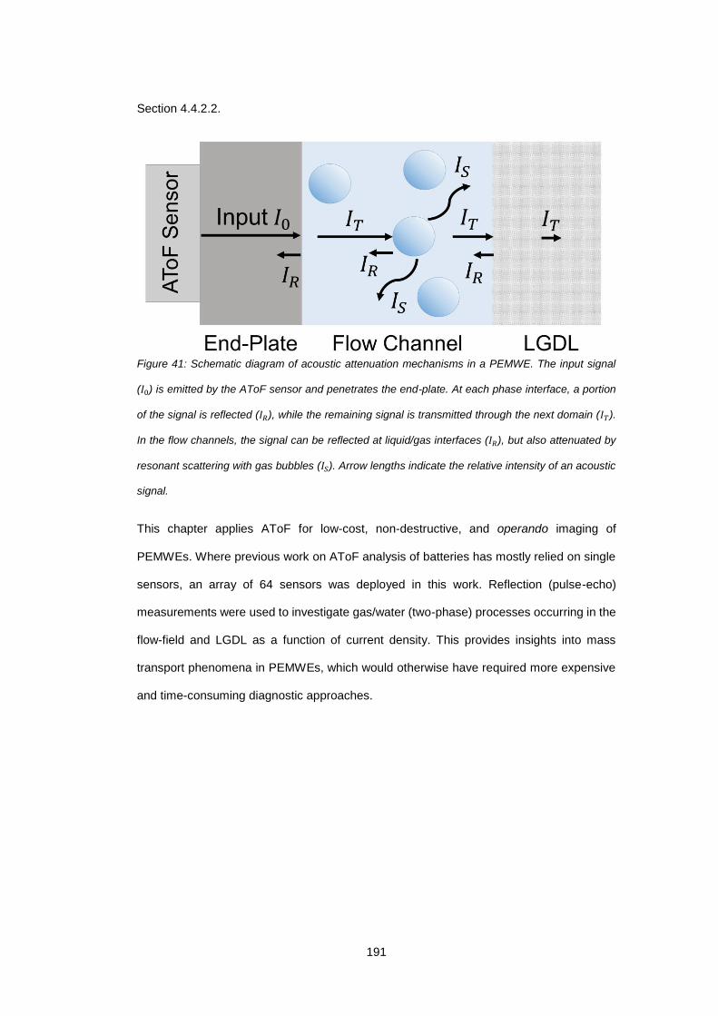
191
Section 4.4.2.2.
Figure 41: Schematic diagram of acoustic attenuation mechanisms in a PEMWE. The input signal
(𝐼0) is emitted by the AToF sensor and penetrates the end-plate. At each phase interface, a portion
of the signal is reflected (𝐼𝑅), while the remaining signal is transmitted through the next domain (𝐼𝑇).
In the flow channels, the signal can be reflected at liquid/gas interfaces (𝐼𝑅), but also attenuated by
resonant scattering with gas bubbles (𝐼𝑆). Arrow lengths indicate the relative intensity of an acoustic
signal.
This chapter applies AToF for low-cost, non-destructive, and operando imaging of
PEMWEs. Where previous work on AToF analysis of batteries has mostly relied on single
sensors, an array of 64 sensors was deployed in this work. Reflection (pulse-echo)
measurements were used to investigate gas/water (two-phase) processes occurring in the
flow-field and LGDL as a function of current density. This provides insights into mass
transport phenomena in PEMWEs, which would otherwise have required more expensive
and time-consuming diagnostic approaches.
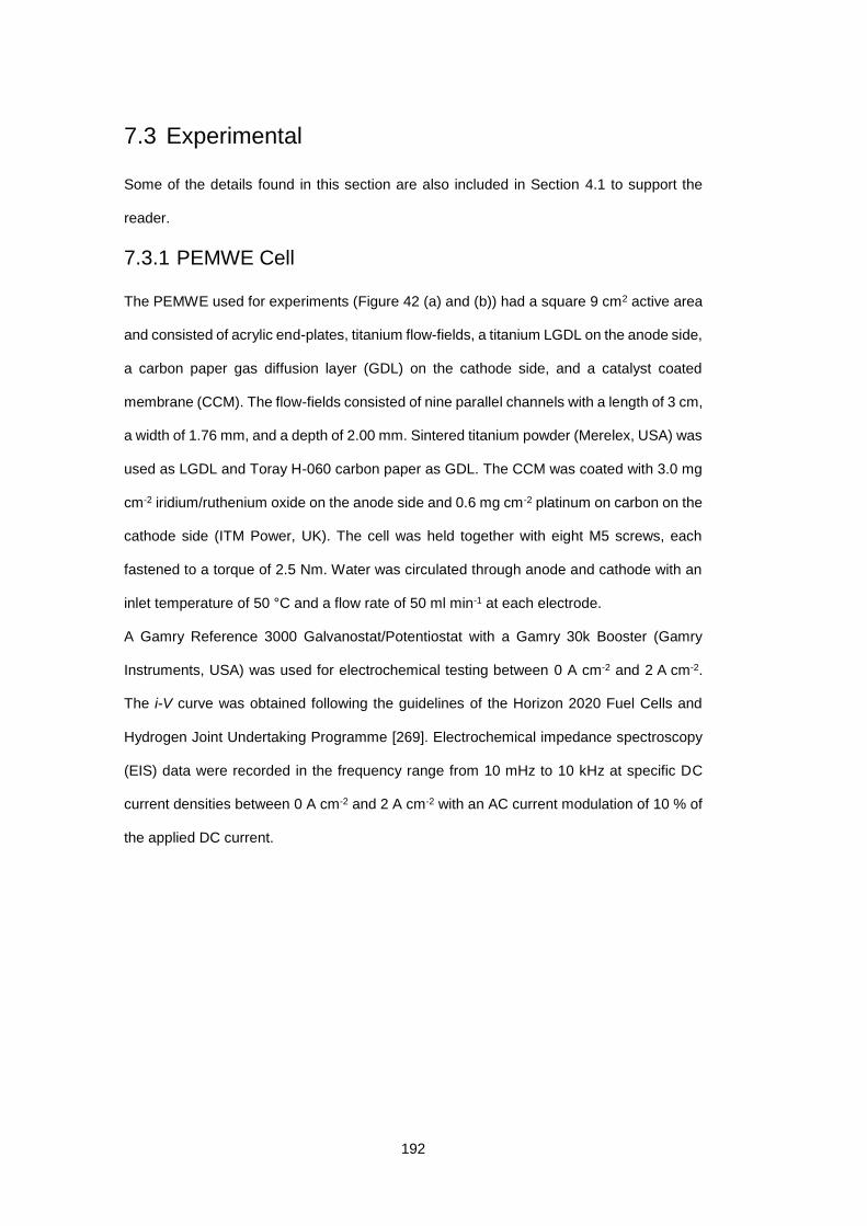
192
7.3 Experimental
Some of the details found in this section are also included in Section 4.1 to support the
reader.
7.3.1 PEMWE Cell
The PEMWE used for experiments (Figure 42 (a) and (b)) had a square 9 cm2 active area
and consisted of acrylic end-plates, titanium flow-fields, a titanium LGDL on the anode side,
a carbon paper gas diffusion layer (GDL) on the cathode side, and a catalyst coated
membrane (CCM). The flow-fields consisted of nine parallel channels with a length of 3 cm,
a width of 1.76 mm, and a depth of 2.00 mm. Sintered titanium powder (Merelex, USA) was
used as LGDL and Toray H-060 carbon paper as GDL. The CCM was coated with 3.0 mg
cm-2 iridium/ruthenium oxide on the anode side and 0.6 mg cm-2 platinum on carbon on the
cathode side (ITM Power, UK). The cell was held together with eight M5 screws, each
fastened to a torque of 2.5 Nm. Water was circulated through anode and cathode with an
inlet temperature of 50 °C and a flow rate of 50 ml min-1 at each electrode.
A Gamry Reference 3000 Galvanostat/Potentiostat with a Gamry 30k Booster (Gamry
Instruments, USA) was used for electrochemical testing between 0 A cm-2 and 2 A cm-2.
The i-V curve was obtained following the guidelines of the Horizon 2020 Fuel Cells and
Hydrogen Joint Undertaking Programme [269]. Electrochemical impedance spectroscopy
(EIS) data were recorded in the frequency range from 10 mHz to 10 kHz at specific DC
current densities between 0 A cm-2 and 2 A cm-2 with an AC current modulation of 10 % of
the applied DC current.
193
Figure 42: (a) The PEMWE setup consists of end-plates, parallel flow-fields, a titanium sintered liquid-
gas diffusion layer (LGDL), the catalyst coated membrane (CCM), and the gas diffusion layer (GDL)
on the cathode side. (b) The AToF sensor array is mounted on the outer surface of the anode end-
plate.
7.3.2 AToF Measurements
All measurements were taken with an array of 64 acoustic sensors in pulse-echo mode on
the anode side of the PEMWE. Each data point was averaged from the signals received
from 16 neighbouring sensors (1-16, 2-17, 3-18, …., 49-64), which is called a ‘sensor unit’.
Each sensor unit recorded one measurement per second. The signal received was the
reflected portion of the input signal, which was a pulse sequence with a maximum repetition
frequency of 20 kHz. All data was amplified before recording. The amplitude of this
amplification is called the acoustic gain. Sensors were controlled and read out with an
Olympus FOCUS PX system (Olympus Scientific Solutions, USA). All AToF data in this
work is given as a percentage of the sensor saturation value. Before each experiment, a
layer of acoustic gel (D12 Couplant Gel, Olympus Scientific Solutions, USA) was applied
to the outer surface of the PEMWE and the sensor. This provided good acoustic coupling
between sensor and PEMWE surface and ensured a consistent signal across the surface.
Two different types of AToF experiments were conducted: fixed position experiments and
area scans. For fixed position experiments, the sensor was mounted to a specific location
and data were recorded continuously while the current density was increased from 0 A cm-2
to 2 A cm-2 in 0.1 A cm-2 increments, each lasting 120 s. Three different locations along the
length of the flow-field were defined, each covering the whole width of the flow-field. The
194
lower location was 0.5 cm from the bottom end of the active area, the upper location 0.5
cm from its top end, and the middle location exactly 1.5 cm from either end of the flow-field.
On the other hand, area scans were performed by moving the sensor array across the
active area (10 mm s-1) from the bottom to the top of the flow channels, while operating the
PEMWE at a constant current density. The sensor array was mounted onto an additional
Rexolite block (thickness: 2 cm) to avoid damaging the sensor surface while gliding it over
the PEMWE surface.
To analyse the acoustic response from different components of the PEMWE, different time-
of-flight intervals of the echo-response were analysed; as the LGDL was located after the
flow-field, peaks at a higher ToF were attributed to the LGDL, lower ToF peaks were
attributed to the flow-field. Experiments were conducted with different acoustic gains (signal
amplification). A clear signal from the anode flow-field was obtained at a gain of 40 dB,
however, this acoustic intensity was not strong enough to obtain a clear reflection signal
from the LGDL. Therefore, experiments were also carried out at a gain of 60 dB, in which
case the signal from the flow-field was saturated, but sufficient signal intensity for analysis
was obtained from the LGDL.
For comparison to AToF measurements of the PEMWE during operation, measurements
of the dry PEMWE cell (without water inflow) at all three different sensor locations were
taken as well.
7.3.3 AToF Data Analysis
Data was visualised in real-time in the FocusPC software (Olympus Scientific Solutions,
USA), which was also used for data export. The FocusPC interface was used to measure
the maximum reflection intensity in time-of-flight intervals containing the reflection peaks
related to specific components of the PEMWE, e.g. flow-fields or the LGDL. The waveform
intervals correlated to components of the PEMWE were chosen manually based on a
number of AToF scans with varying parameters. Subsequently, the peak intensity was
recorded for each sensor unit and throughout the duration of the experiment. More details
on AToF data analysis can be found in Section 4.4.4.
The resulting data points were mapped and analysed qualitatively and quantitatively. Each
195
peak of the waveform (intensity value in an acoustic map) is caused by the reflection of the
acoustic input signal at an interface. The intensity of a reflection peak relates to the fraction
of signal which is reflected at a given interface (the acoustic reflection 𝑅), which is a function
of the acoustic impedances of the adjacent phases (see Section 4.4.2.2).
Understanding the causes of reflection in a system enables an understanding of the nature
of an interface from observing the intensity of the recorded reflection peaks. However, the
pulse-echo signal is not only influenced by reflection at interfaces, but also by resonant
scattering. This occurs when an acoustic wave travels through a medium containing gas
bubbles (such as water in the flow channels of a PEMWE). If the frequency of the wave is
at or near the resonance frequency of a gas bubble, a major fraction of the wave is
scattered. However, during operation of a PEMWE, a multitude of gas bubbles are
produced, covering a wide range of bubble sizes, hence, a wide range of frequencies exist
within which resonant scattering between acoustic wave and bubbles can occur. The flow-
channels of a PEMWE under operation therefore strongly attenuate the AToF signal and
the degree of attenuation of the signal in the flow channels is a measure of the amount of
gas being transported. Details on the scattering frequency of individual gas bubbles and
bubble clouds are found in Section 4.4.2.2 and were used in the following for data
interpretation.
To obtain frequency information from the pulse-echo response, fast Fourier transform
(FFT) analysis of the AToF waveform was performed using the FocusPC software. The
pulse-echo response across the entire time-of-flight was analysed, yielding an intensity
spectrum as a function of frequency. The frequency at which the maximum intensity was
found, will be referred to as peak frequency in the following. Comparison of the peak
frequency with values obtained from the equations in Section 4.4.2.2 serves to indicate
whether the obtained signal predominantly originated from resonant scattering.
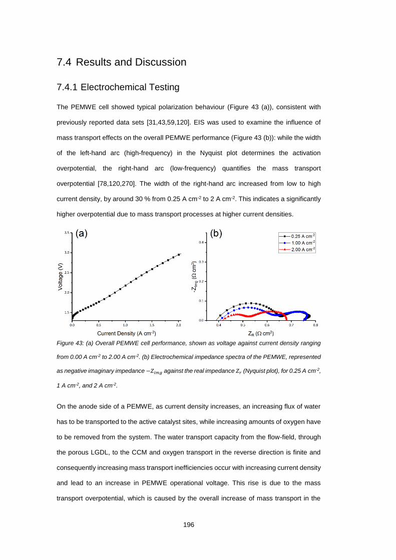
196
7.4 Results and Discussion
7.4.1 Electrochemical Testing
The PEMWE cell showed typical polarization behaviour (Figure 43 (a)), consistent with
previously reported data sets [31,43,59,120]. EIS was used to examine the influence of
mass transport effects on the overall PEMWE performance (Figure 43 (b)): while the width
of the left-hand arc (high-frequency) in the Nyquist plot determines the activation
overpotential, the right-hand arc (low-frequency) quantifies the mass transport
overpotential [78,120,270]. The width of the right-hand arc increased from low to high
current density, by around 30 % from 0.25 A cm-2 to 2 A cm-2. This indicates a significantly
higher overpotential due to mass transport processes at higher current densities.
Figure 43: (a) Overall PEMWE cell performance, shown as voltage against current density ranging
from 0.00 A cm-2 to 2.00 A cm-2. (b) Electrochemical impedance spectra of the PEMWE, represented
as negative imaginary impedance −𝑍𝑖𝑚𝑔 against the real impedance 𝑍𝑟 (Nyquist plot), for 0.25 A cm-2,
1 A cm-2, and 2 A cm-2.
On the anode side of a PEMWE, as current density increases, an increasing flux of water
has to be transported to the active catalyst sites, while increasing amounts of oxygen have
to be removed from the system. The water transport capacity from the flow-field, through
the porous LGDL, to the CCM and oxygen transport in the reverse direction is finite and
consequently increasing mass transport inefficiencies occur with increasing current density
and lead to an increase in PEMWE operational voltage. This rise is due to the mass
transport overpotential, which is caused by the overall increase of mass transport in the

197
PEMWE system.
7.4.2 Structural Investigation with AToF
The ability of acoustic waves to penetrate through layers of material can be used for rapid
inspection and diagnostics. AToF scanning of the entire active area (as described in
Section 7.3.2) provided a spatially resolved 3D imaging technique, visualising the structure
of different PEMWE components. Experiments at two different acoustic gains were used to
investigate the structure and assembly of flow-field and LGDL in the PEMWE. Each AToF
experiment offered depth-profiling of the same layers of the PEMWE, such as flow-field
and LGDL, but investigation of different layers was carried out in separate experiments to
obtain an optimal and clear signal from each component. The PEMWE was operated at
0.25 A cm-2 for both experiments, hence water and oxygen gas both exist in flow-field as
well as the pore phase of the LGDL. Based on preliminary experiments, different time-of-
flight intervals were chosen for each component, measuring the maximum reflection peak
intensity in the respective interval.
The structure of the flow-field was visualized with AToF, showing details of the flow
channels, the ribs and water inlet and outlet. A low reflective peak was observed in channel
areas (blue areas in Figure 44 (a)), while the ribs were marked by high reflective peaks
(yellow areas). Comparison between the actual geometry of the parallel flow-field (Figure
44 (b)) with the AToF image showed that all eight ribs and nine channels were detected.
The ratio between rib length and width was 17.05 for the actual flow-field design, and was
manually measured to be 18.70 from the AToF image. Based on the width of the active
area (30 mm, 32 pixel) a spatial resolution of 0.94 mm was obtained. The fact that high
reflection intensities were detected in the rib areas, while lower intensities were found in
the channel areas, suggests that the acoustic impedance of the acrylic end-plate was more
closely matched with the acoustic impedance of the water-filled channels than with the
acoustic impedance of the titanium flow-field ribs. This might seem counter-intuitive, but
can be derived from the material values (Section 4.4.2.2). Further, the very low reflection
intensity in the flow channels is likely to be attributed to resonant scattering from oxygen
bubbles. This will be further validated in Section 7.4.3.
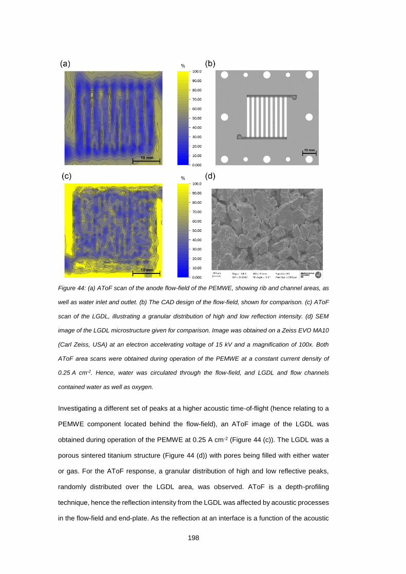
198
Figure 44: (a) AToF scan of the anode flow-field of the PEMWE, showing rib and channel areas, as
well as water inlet and outlet. (b) The CAD design of the flow-field, shown for comparison. (c) AToF
scan of the LGDL, illustrating a granular distribution of high and low reflection intensity. (d) SEM
image of the LGDL microstructure given for comparison. Image was obtained on a Zeiss EVO MA10
(Carl Zeiss, USA) at an electron accelerating voltage of 15 kV and a magnification of 100x. Both
AToF area scans were obtained during operation of the PEMWE at a constant current density of
0.25 A cm-2. Hence, water was circulated through the flow-field, and LGDL and flow channels
contained water as well as oxygen.
Investigating a different set of peaks at a higher acoustic time-of-flight (hence relating to a
PEMWE component located behind the flow-field), an AToF image of the LGDL was
obtained during operation of the PEMWE at 0.25 A cm-2 (Figure 44 (c)). The LGDL was a
porous sintered titanium structure (Figure 44 (d)) with pores being filled with either water
or gas. For the AToF response, a granular distribution of high and low reflective peaks,
randomly distributed over the LGDL area, was observed. AToF is a depth-profiling
technique, hence the reflection intensity from the LGDL was affected by acoustic processes
in the flow-field and end-plate. As the reflection at an interface is a function of the acoustic
199
impedance of both materials at this interface, the acoustic response from LGDL pores and
particles was different in rib and land areas. This makes it difficult to clearly assign low or
high reflection peaks to either pores or particles. Further, the granularity of the AToF
response was much coarser than the microstructure of the LGDL. As observed above, the
spatial resolution of the AToF measurement is 0.94 mm, while the size of pores and
particles of the LGDL are significantly smaller (Figure 44 (d)). This suggests that with the
given experimental equipment AToF cannot be used to distinguish individual pores or
particles, but rather larger accumulations of gas or water in a network of adjacent pores.
However, by observing the overall reflection intensity as a function of current density,
conclusions can be drawn on the volume averaged macroscopic processes in the LGDL
(Section 7.4.3.2).
The above results show that AToF scans are a powerful 3D imaging and depth-profiling
tool for quick inspection and qualitative analysis. However, to obtain quantitative data as a
function of current density, fixed position AToF measurements are also investigated below
to reduce any error that may be introduced while moving the acoustic sensor.
7.4.3 AToF for Quantitative Assessment
By applying AToF across the whole width of the active area at a fixed location, while varying
current density, statistically reliable data (probing of a constant state of operation for 120
s) on the acoustic response was obtained. Experiments were conducted at three different
sensor locations (lower, middle, and upper as defined in Section 7.3.2) and two different
acoustic time-of-flight intervals to access the flow-field and LGDL, respectively.
7.4.3.1 Flow-Field
Figure 45 (a) shows the AToF response from the flow-field at the middle location on a
logarithmic scale between 0 A cm-2 and 2 A cm-2, hence, illustrating the evolution of the
reflection intensity in the middle segment of the flow-field across the entire active area (and
all flow channels and ribs) as a function of current density. To visualize the large relative
changes in intensity across the current density range, the use of a logarithmic scale was
required. A general trend from high reflection intensity to low reflection intensity was
observed as current density was increased. While the average intensity of the flow-field
200
reflection peaks was around 55 % at 0 A cm-2, it dropped to 5 % at 2 A cm-2. At 0 A cm-2,
the AToF signal was reflected at the interface between the end-plate and flow
channels/ribs. Due to the mismatch in physical properties, and hence acoustic impedance,
the transition from end-plate to water in the flow channels produced a strong reflection
peak. As current density increased, the flow channels were not only filled with water, but
also with an increasing amount of oxygen bubbles. As outlined in Section 4.4.2.2, gas
bubbles attenuate the AToF signal via resonant scattering. This explains why the averaged
intensity decreased continuously with increasing current density. As more gas was
produced, the acoustic input wave was scattered (anisotropically) more strongly, which
reduced the intensity of the echo signal detected.
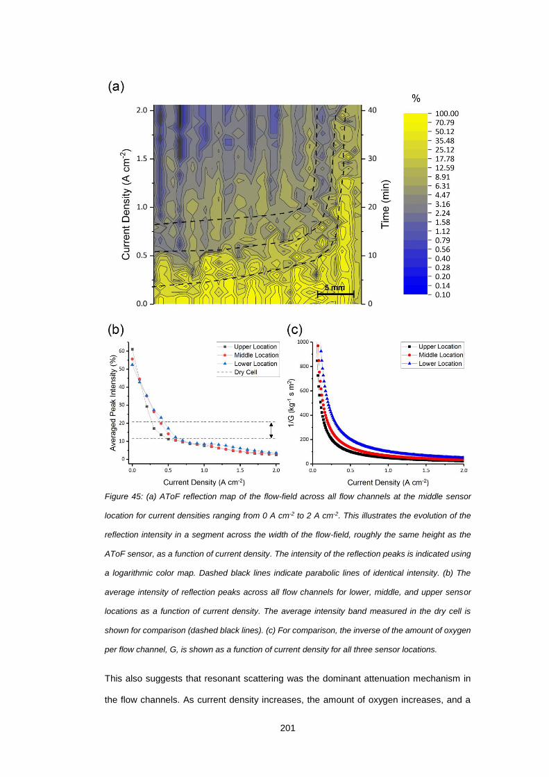
201
Figure 45: (a) AToF reflection map of the flow-field across all flow channels at the middle sensor
location for current densities ranging from 0 A cm-2 to 2 A cm-2. This illustrates the evolution of the
reflection intensity in a segment across the width of the flow-field, roughly the same height as the
AToF sensor, as a function of current density. The intensity of the reflection peaks is indicated using
a logarithmic color map. Dashed black lines indicate parabolic lines of identical intensity. (b) The
average intensity of reflection peaks across all flow channels for lower, middle, and upper sensor
locations as a function of current density. The average intensity band measured in the dry cell is
shown for comparison (dashed black lines). (c) For comparison, the inverse of the amount of oxygen
per flow channel, G, is shown as a function of current density for all three sensor locations.
This also suggests that resonant scattering was the dominant attenuation mechanism in
the flow channels. As current density increases, the amount of oxygen increases, and a
202
number of flow regimes is typically observed in the flow channels. It is well-established that
at low current densities the bubbly flow regime is observed, which then consecutively
develops into slug and annular flow with increasing current density and location along any
given flow channel [40]. Due to the large number of individual bubbles [218], the bubbly
regime exhibits by far the highest amount of liquid/gas and gas/solid interfaces. If acoustic
reflection at interfaces were to be the dominant attenuation mechanism, a maximum of
reflection would be expected in the bubbly regime, with a decrease in reflection intensity
for higher current densities due to the reduction in interfaces and the increasing amount of
resonant scattering. However, as a continuous decrease in reflection intensity was
observed experimentally, it appears likely that the dominant mechanism of acoustic
attenuation in the flow channels was resonant scattering.
To establish the link between oxygen gas production and AToF signal, the pulse-echo
response averaged across all channels (Figure 45 (b)) and the inverse (increasing gas flow
reduces the reflection intensity) of the gravimetric gas flow per flow channel, G, (Figure 45
(c)) are displayed as a function of current density. The gas flow was calculated theoretically
based on Faraday’s law [40,218]. The different gas flows at the sensor locations was
accounted for by adapting the active area used for the calculation, according to the location
of the sensor along the flow channels. The pulse-echo response showed a continuous
decrease with current density, which mirrors the behaviour of the inverse oxygen flow 1 𝐺⁄ .
An initial drop at low current densities was followed by a linear decrease from around
0.5 A cm-2 to 2 A cm-2. The distance between the curves for different locations was not as
pronounced for the pulse-echo response as for the calculated inverse gas flow. This implies
that attenuation due to resonant scattering was the dominant mechanism. However, it was
convoluted by other attenuation mechanisms, such as reflection from gas/liquid and
liquid/solid interfaces.
This was further supported by comparing the average reflection intensity in the flow
channels under operation and in the completely dry cell. The band of average reflection
intensity (two standard deviations) ranged between 11.46 % and 20.75 % (dashed black
lines in Figure 45 (b)) for AToF measurements of the cell completely filled with air and void
of water. However, the dry reflection intensity was considerably higher than values obtained
203
during PEMWE operation at current densities beyond 0.75 A cm-2, where the flow channels
contained a water-gas mixture. Hence, the signal attenuation in the flow channels could
not be solely caused by the reflection at the gas interface. It is therefore implied that
resonant scattering caused the unexpectedly low reflection intensity values.
Another feature of the AToF signal was that it exhibited an approximately parabolic profile
across the flow channels. From left to right, the transition from a given acoustic intensity
level to a lower one (e.g. yellow to blue in Figure 45 (a)) occurred at an increasingly high
current density. Therefore, the lines of equal AToF intensity (black dashed lines in Figure
45 (a)) formed a parabolic profile roughly increasing from left to right. The effect of non-
uniform flow distribution, following a parabolic profile, in a parallel flow-field is well
documented [72,75,76] and has been observed with optical imaging of the PEMWE flow
channels [73]. This is a consequence of the flow-field being designed in a Z-pattern, with
water inlet and outlet being located at diagonally opposed ends of the parallel flow-field,
which causes the water flow rate to be higher in the channels to the right (closer to the
outlet) by a factor of up to five compared to the remainder of the channels [72]. This further
established the ability of AToF to represent the physical processes in the flow-field.
To further confirm resonant scattering as a dominant force of acoustic attenuation in the
flow channels, for the middle location, the calculated frequencies for resonant scattering
were compared with the peak of the signal frequency spectrum obtained via FFT (Figure
46). The frequency of resonant scattering was calculated as a function of current density
(as described in Section 4.4.2.2), using a mass balance and Faraday’s law to determine
the gas fraction [40,218]. For the middle location, the active area was assumed to be half
of the entire active area, thus only accounting for the amount of gas that had accumulated
in the flow channels at the middle sensor location. Assuming the bubble cloud diameter
being equal to the width of a flow channel, the resonant frequency is trending towards
infinite values for 0 A cm-2 and falls to around 0.50 MHz at 2 A cm-2. Additionally, the
frequency of peak intensity was determined from the AToF signal for each current density
via FFT analysis of the waveform along the entire observed time-of-flight. This indicated
the most common echo-signal frequency occurring in the PEMWE and was linked to the
processes causing the echo-response. The peaks related to the flow channels were by far
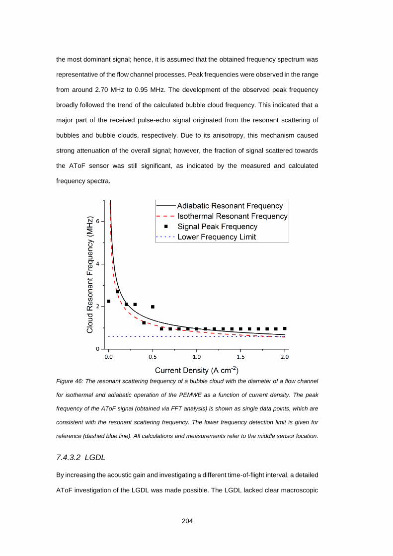
204
the most dominant signal; hence, it is assumed that the obtained frequency spectrum was
representative of the flow channel processes. Peak frequencies were observed in the range
from around 2.70 MHz to 0.95 MHz. The development of the observed peak frequency
broadly followed the trend of the calculated bubble cloud frequency. This indicated that a
major part of the received pulse-echo signal originated from the resonant scattering of
bubbles and bubble clouds, respectively. Due to its anisotropy, this mechanism caused
strong attenuation of the overall signal; however, the fraction of signal scattered towards
the AToF sensor was still significant, as indicated by the measured and calculated
frequency spectra.
Figure 46: The resonant scattering frequency of a bubble cloud with the diameter of a flow channel
for isothermal and adiabatic operation of the PEMWE as a function of current density. The peak
frequency of the AToF signal (obtained via FFT analysis) is shown as single data points, which are
consistent with the resonant scattering frequency. The lower frequency detection limit is given for
reference (dashed blue line). All calculations and measurements refer to the middle sensor location.
7.4.3.2 LGDL
By increasing the acoustic gain and investigating a different time-of-flight interval, a detailed
AToF investigation of the LGDL was made possible. The LGDL lacked clear macroscopic
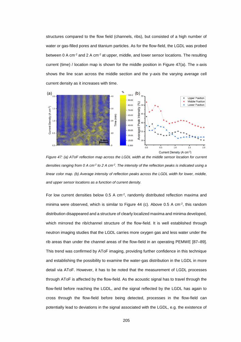
205
structures compared to the flow field (channels, ribs), but consisted of a high number of
water or gas-filled pores and titanium particles. As for the flow-field, the LGDL was probed
between 0 A cm-2 and 2 A cm-2 at upper, middle, and lower sensor locations. The resulting
current (time) / location map is shown for the middle position in Figure 47(a). The x-axis
shows the line scan across the middle section and the y-axis the varying average cell
current density as it increases with time.
Figure 47: (a) AToF reflection map across the LGDL width at the middle sensor location for current
densities ranging from 0 A cm-2 to 2 A cm-2. The intensity of the reflection peaks is indicated using a
linear color map. (b) Average intensity of reflection peaks across the LGDL width for lower, middle,
and upper sensor locations as a function of current density.
For low current densities below 0.5 A cm-2, randomly distributed reflection maxima and
minima were observed, which is similar to Figure 44 (c). Above 0.5 A cm-2, this random
distribution disappeared and a structure of clearly localized maxima and minima developed,
which mirrored the rib/channel structure of the flow-field. It is well established through
neutron imaging studies that the LGDL carries more oxygen gas and less water under the
rib areas than under the channel areas of the flow-field in an operating PEMWE [87–89].
This trend was confirmed by AToF imaging, providing further confidence in this technique
and establishing the possibility to examine the water-gas distribution in the LGDL in more
detail via AToF. However, it has to be noted that the measurement of LGDL processes
through AToF is affected by the flow-field. As the acoustic signal has to travel through the
flow-field before reaching the LGDL, and the signal reflected by the LGDL has again to
cross through the flow-field before being detected, processes in the flow-field can
potentially lead to deviations in the signal associated with the LGDL, e.g. the existence of
206
rib/channel features in the AToF response from the LGDL can potentially be an artefact
caused by the input signal being transmitted through the flow-field before penetrating the
LGDL.
The overall intensity of reflection peaks attributed to the LGDL decreased with increasing
current density (Figure 47 (b)). The variance between individual locations is likely caused
by differences in local porosity of the LGDL and the formation of gas and water pathways
in specific areas. A decrease from around 52 % acoustic intensity at 0 A cm-2 to around
38 % at 2 A cm-2 was observed for the middle position. However, the typical decrease in
reflection peaks with current density was considerably smaller in the LGDL than in the flow
channels. Other than in the flow-field, where almost the entire channel was filled with gas
at high current density, in the LGDL only certain parts of the porosity of the LGDL contained
gas at any given time. The remainder consisted of solid titanium and water pathways, which
change little with current density.
The development of reflection intensity with current density observed here is consistent
with through-plane water thickness measurements performed using neutron imaging [90],
which will be presented in Section 5. Neutron imaging can reliably measure the absolute
water thickness in a sample due to the strong interactions of neutrons with hydrogen atoms
and therefore data on the water thickness in the LGDL obtained via neutron imaging can
be used for validation and calibration of AToF data. As shown in Section 5, a decrease in
water thickness by 12 % between 0.25 A cm-2 and 1.5 A cm-2 was found averaged across
all rib areas using the same LGDL material as this work. This compares to a decrease of
13 % in reflection intensity across the active area found in this work between 0.2 A cm-2
and 1.5 A cm-2. The close correlation in neutron imaging data and AToF response
emphasized the possibility of applying AToF imaging to LGDL processes and validated the
chosen methodology.
207
7.5 Conclusion
This work establishes AToF imaging as a promising diagnostic tool for PEMWEs, however,
the resolution limitations outlined in Section 7.4.2 have to be considered carefully when
applying AToF imaging. It is demonstrated that the internal structure and assembly of flow-
field and LGDL can be visualized using AToF scans across the PEMWE active area. This
can be used for rapid, non-destructive inspection and diagnosis of PEMWE systems and
offers a much lower cost and easily deployable operando imaging capability than
established methods, such as X-ray or neutron imaging. By measuring the pulse-echo
response of a PEMWE operated between 0 A cm-2 and 2 A cm-2 a range of effects typical
for PEMWEs have been observed, which corroborates the effectiveness of AToF imaging.
These effects were related to the flow-field as well as the LGDL.
Acoustic investigation of the flow-field showed a general decrease in reflection intensity
with increasing current density. This indicates an increasing acoustic attenuation, which is
caused by the increasing amount of oxygen gas produced and removed through the flow
channels. It is shown by calculating the amount of oxygen produced due to electrochemical
activity that the AToF signal scales closely with the inverse of the amount of gas in the flow
channels. By determining the peak frequency of the AToF signal as a function of current
density using FFT analysis, and comparing these data with theoretical expectations for the
frequency of resonant scattering of bubbles, the link between gas bubbles in the flow
channels and acoustic attenuation was confirmed. Further, AToF imaging yielded a
parabolic profile of intensity across the flow channels, an effect well established in the
literature, which corroborates the validity of the data obtained in this work.
AToF imaging of the LGDL showed a granular distribution of reflection maxima and minima.
However, the spatial resolution of the AToF equipment was not sufficient to resolve the
LGDL microstructure of gas/water pathways and titanium particles. Just as for the flow-
field, a general trend of decreasing reflection intensity with increasing current density was
observed between 0 A cm-2 and 2 A cm-2. However, the trend was less pronounced than
for the flow-field. It was demonstrated that the AToF response scales closely to data on the
water thickness in the identical LGDL material, obtained via neutron imaging. Further, AToF
208
imaging showed a distinct difference between areas of the LGDL under rib and land areas
of the flow-field, respectively. This can potentially be attributed to the accumulation of gas
and water under rib and channels of the flow-field, respectively. This effect has been well
documented by neutron imaging. Overall, this confirms the ability of AToF imaging to
investigate macroscopic processes in the LGDL.
In conclusion, it was demonstrated that AToF imaging is well suited to investigate mass
transport processes in flow-field as well as the LGDL of PEMWEs. It offers a low-cost,
rapid, non-destructive, operando imaging tool. In a research context, it can potentially
replace more time-consuming, expensive and specialized investigation techniques such as
neutron and X-ray imaging. Commercial applications could include rapid inspection of
single cells and PEMWE stacks or the diagnosis of non-uniform distribution of reactants
across the active area, which could indicate faulty cell assembly or issues related to the
CCM.

209
8 Future Work


211
8.1 Overview
This section will outline a number of experimental plans, which naturally follow from the
ideas and results outlined in this work. In some cases, preliminary results are shown to
demonstrate the feasibility or value of these projects, which would form a good starting
point for postdoctoral research or a PhD project.
212
8.2 Novel Engineering Approaches
One of the key conclusions from this work is that the established designs and materials
used for PEMWEs come with a number of disadvantages and are not optimized for mass
transport under high current density. This calls for novel approaches to the design of LGDL
and flow-fields, using well-defined structures instead of naturally available materials (e.g.
sintered powder), and tailoring geometries to optimize mass transport.
8.2.1 Additive Manufacturing of LGDLs
In recent years, additive manufacturing (‘3D printing’) has become one of the most
promising approaches for manufacturing of novel structures for energy-related structures,
such as battery or supercapacitor electrodes, electronic circuits, or flexible lighting [271].
Additive manufacturing usually refers to extrusion-type 3D printing; however, it also
encompasses selective laser sintering (SLS), selective laser melting (SLM), and electron
beam melting (EBM), which are used to 3D print metal structures from a bed of metal
powder. These processes have successfully been used to 3D print PEMWE components,
such as titanium LGDLs [272], stainless steel flow-plates [62,273], and stainless steel
plates integrating flow-field and LGDL in one component [51].
The versatility of 3D printing can also be used to create LGDL structures with tailored pore
shapes and hydrophilicity. Additive manufacturing offers the capability of creating LGDLs
with conical pores, hence manipulating the contact angle between pore wall and water.
This results in tuneable hydrophilicity of the pore and allows to distribute pores with
modified water contact angle across the active area, therefore allowing for a targeted
distribution of water to achieve optimized water ingress and equilibration of non-uniform
distribution of reactants or current density across the active area.
8.2.1.1 Preliminary Results
To gain a first impression of the influence of the pore shape on mass transport in a PEMWE,
three titanium LGDL (Thickness: 1 mm) were designed and manufactured (Protolabs, UK):
one with straight, cylindrical pores (Figure 48 (b)), one with conical pores opening towards
the CCM (Figure 48 (c)), and one with conical pores opening towards the flow channels
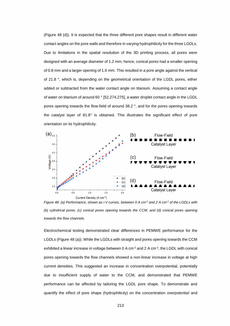
213
(Figure 48 (d)). It is expected that the three different pore shapes result in different water
contact angles on the pore walls and therefore in varying hydrophilicity for the three LGDLs.
Due to limitations in the spatial resolution of the 3D printing process, all pores were
designed with an average diameter of 1.2 mm; hence, conical pores had a smaller opening
of 0.8 mm and a larger opening of 1.6 mm. This resulted in a pore angle against the vertical
of 21.8 °, which is, depending on the geometrical orientation of the LGDL pores, either
added or subtracted from the water contact angle on titanium. Assuming a contact angle
of water on titanium of around 60 ° [52,274,275], a water droplet contact angle in the LGDL
pores opening towards the flow-field of around 38.2 °, and for the pores opening towards
the catalyst layer of 81.8° is obtained. This illustrates the significant effect of pore
orientation on its hydrophilicity.
Figure 48: (a) Performance, shown as i-V curves, between 0 A cm-2 and 2 A cm-2 of the LGDLs with
(b) cylindrical pores, (c) conical pores opening towards the CCM, and (d) conical pores opening
towards the flow channels.
Electrochemical testing demonstrated clear differences in PEMWE performance for the
LGDLs (Figure 48 (a)). While the LGDLs with straight and pores opening towards the CCM
exhibited a linear increase in voltage between 0 A cm-2 and 2 A cm-2, the LGDL with conical
pores opening towards the flow channels showed a non-linear increase in voltage at high
current densities. This suggested an increase in concentration overpotential, potentially
due to insufficient supply of water to the CCM, and demonstrated that PEMWE
performance can be affected by tailoring the LGDL pore shape. To demonstrate and
quantify the effect of pore shape (hydrophilicity) on the concentration overpotential and
214
PEMWE performance, a systematic study, examining a wide range of 3D printed LGDLs
with different pore shapes and sizes, would be required to ensure that the performance
effect observed above is due to a change in mass transport, and not the variation of other
parameters such as the available triple-phase boundary.
The electrochemical performance of the LGDLs tested here is poor, with voltages
exceeding 4 V at 2 A cm-2. However, due to the limitations on the minimum achievable
feature size of the additive manufacturing process, the LGDL pores were large compared
to the pore sizes of commonly deployed materials (e.g. 20 µm to 140 µm for a typical
titanium felt, see Section 5.4.1). Therefore, the high operational voltage observed here is
likely due to a lack of triple-phase boundary, but can be improved upon by creating LGDL
structures with smaller pores. As additive manufacturing technology is constantly evolving
[276], it is likely that such structures can be manufactured in the future.
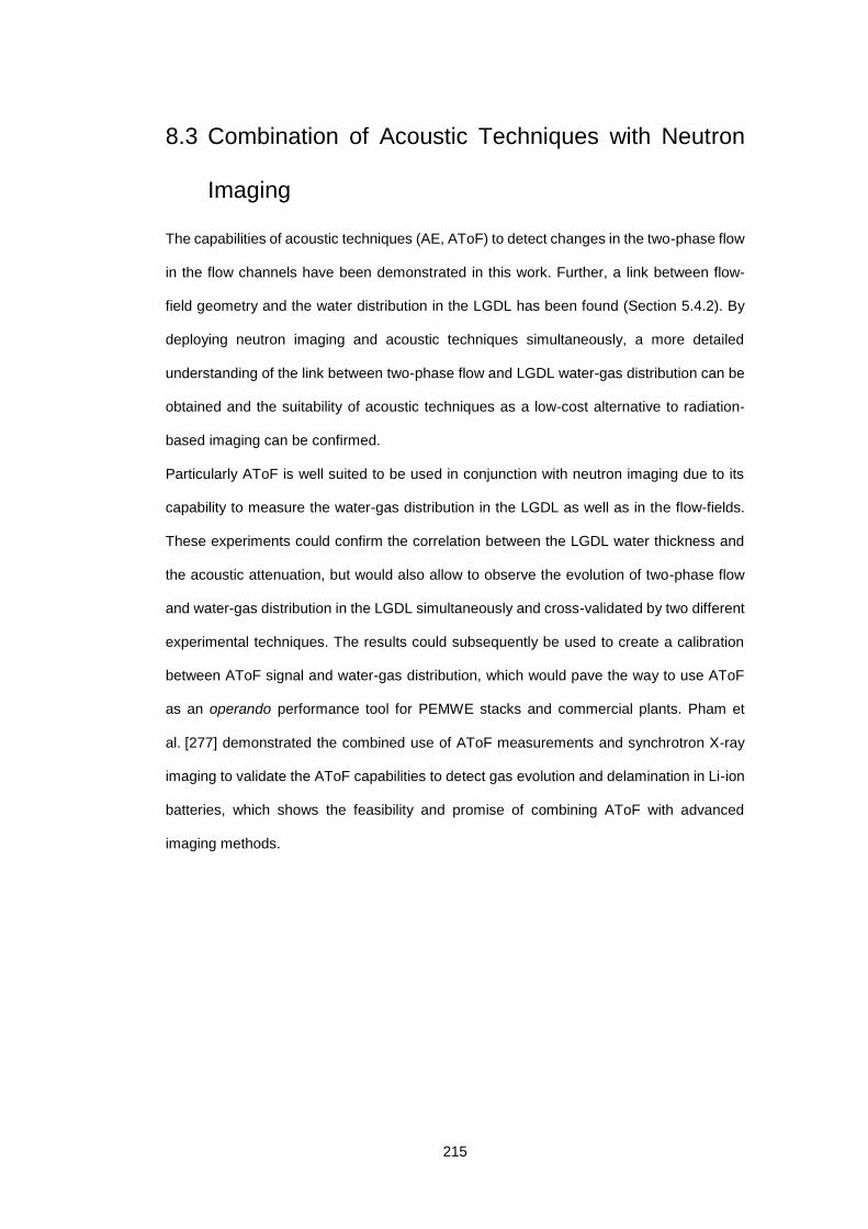
215
8.3 Combination of Acoustic Techniques with Neutron
Imaging
The capabilities of acoustic techniques (AE, AToF) to detect changes in the two-phase flow
in the flow channels have been demonstrated in this work. Further, a link between flow-
field geometry and the water distribution in the LGDL has been found (Section 5.4.2). By
deploying neutron imaging and acoustic techniques simultaneously, a more detailed
understanding of the link between two-phase flow and LGDL water-gas distribution can be
obtained and the suitability of acoustic techniques as a low-cost alternative to radiation-
based imaging can be confirmed.
Particularly AToF is well suited to be used in conjunction with neutron imaging due to its
capability to measure the water-gas distribution in the LGDL as well as in the flow-fields.
These experiments could confirm the correlation between the LGDL water thickness and
the acoustic attenuation, but would also allow to observe the evolution of two-phase flow
and water-gas distribution in the LGDL simultaneously and cross-validated by two different
experimental techniques. The results could subsequently be used to create a calibration
between AToF signal and water-gas distribution, which would pave the way to use AToF
as an operando performance tool for PEMWE stacks and commercial plants. Pham et
al. [277] demonstrated the combined use of AToF measurements and synchrotron X-ray
imaging to validate the AToF capabilities to detect gas evolution and delamination in Li-ion
batteries, which shows the feasibility and promise of combining AToF with advanced
imaging methods.

216
8.4 Investigation of the Influence of Flow-Field Geometry
on the Water-Gas Distribution in the Liquid-Gas
Diffusion Layer
Results in Section 5 indicate a link between flow-field geometry and the water-gas
distribution in the LGDL underneath the flow-field. This correlation can be further
investigated by a systematic study using neutron imaging to compare the water thickness
distribution in x- and y-direction in the LGDL when using different flow-field geometries
(parallel, single-serpentine, triple-serpentine).
It is expected that areas of the flow channels with a high gas fraction, such as the upper
regions in a parallel flow-field, also exhibit increased gas fractions (decreased through-
plane water thickness) in the areas of the LGDL underneath those areas.
By comparing the water-gas distribution with the flow velocity and distribution of water and
gas in the flow channels adjacent to specific areas in the LGDL, the extent and nature of
the influence of flow-field processes on mass transport in the LGDL can be established.
This would introduce the mass transport characteristics of a flow-field as a novel parameter
to consider in optimizing cell assembly, besides established factors such as pressure drop
and contact resistance with the LGDL.
217
8.5 Investigation of the Link between Flow Regime and
PEMWE Performance
As outlined in Section 3.2.4, uncertainty remains on whether the flow regime in the flow
channels has an influence on PEMWE performance and the nature of this influence. While
there is experimental evidence suggesting that flow regimes with a low water-to-gas ratio,
such as plug or slug flow, cause a decrease in performance [40–42], it has also been
argued that PEMWE performance might improve in slug flow [43,44].
However, to the author’s knowledge, no systematic study comparing PEMWE performance
under a wide range of water and gas flows has been performed yet. By injecting oxygen
upstream of the PEMWE anode, the amount of gas in the flow channels can be controlled
and specific flow regimes achieved (see Figure 49). Varying the amount of injected gas, as
well as the amount of circulated water, PEMWE performance and EIS spectra could be
acquired in a very wide range, covering all relevant flow regimes.
Further, AE sensors can be used to detect and quantify the flow regime in different locations
across the PEMWE active area while varying water flow and gas injection. This would allow
to reliably quantify the two-phase flow and obtain a clear link between performance and
flow regime.
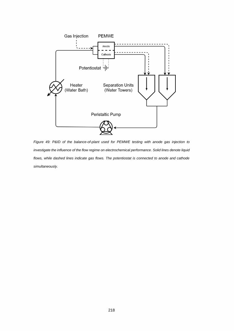
218
Figure 49: P&ID of the balance-of-plant used for PEMWE testing with anode gas injection to
investigate the influence of the flow regime on electrochemical performance. Solid lines denote liquid
flows, while dashed lines indicate gas flows. The potentiostat is connected to anode and cathode
simultaneously.
219
8.6 Conclusion
The rise of renewable energy sources as widespread alternative to conventional energy
production methods and an established part in the energy mix of industrial nations brings
the need for electricity grid stabilization and balancing. Excess energy requires storage,
which can be subsequently released in case of insufficient energy production. A multitude
of mechanical and electrochemical technologies offer this capability, with pumped
hydroelectric systems being by far the most commercially developed system. Due to its
limitation to specific geographic conditions, the use of other energy storage systems is
inevitable.
Among candidate technologies, hydrogen-based solutions are promising and large-scale
projects have been realised. Excess energy is used to produce hydrogen via water
electrolysis, which can subsequently be stored, injected into the gas grid or converted back
into energy using fuel cells. For electrolysis and fuel cells, PEM technology has gained
notable traction due to its advantages over alkaline systems. PEMWEs offer high attainable
current density of 2 A cm-2 and beyond, a more compact build than alkaline water
electrolysis, and low gas crossover.
As PEMWEs grow more mature, the operational current density is further increasing, which
requires increasing amounts of reactants being transported to, from and within a PEMWE
cell. This calls for the adequate design of PEMWE cells so as to ensure sufficient supply
with water and removal of oxygen on the anode side. Inhomogeneity of reactant transport
has to be avoided to prevent local membrane dry-out or hotspot formation. Historically,
there has been little scientific interest for mass transport processes in PEMWEs compared
to electrocatalyst and membrane development, with a lack of understanding of processes
in key components such as flow-fields and LGDL, and few low-cost, operando, and non-
destructive diagnostic tools available.
Therefore, the goal of this thesis was to develop a more thorough understanding of the
mass transport processes in LGDL and flow-fields and develop a suite of diagnostic tools,
facilitating rapid and low-cost investigation of these processes. Due to the very high
attenuation of neutrons in water, neutron imaging was selected to gain insight into the
220
water-gas distribution in the LGDL. Acoustic methods were, to the author’s knowledge,
applied for the first time to PEMWEs in a quest to develop more cost-effective and readily
available diagnostic tools for mass transport processes in PEMWEs, offering an alternative
to established methods like radiation-based imaging.
After outlining the necessary theoretical background, reviewing the available literature
focussed on mass transport processes, and outlining the experimental methodology
employed in this work (Sections 2 to 4), a number of results obtained over the course of
this work are presented. In Section 5, results on the water-gas distribution in the LGDL,
obtained with neutron imaging, are presented. In a first step, measurements of the through-
plane water thickness are correlated to an in-depth study of the LGDL microstructure using
X-ray computed tomography. A clear link between microstructure and water saturation is
shown, and the results indicate a link between flow-field geometry and LGDL water content.
To establish a suite of low-cost diagnostic tools as an alternative to less cost-effective and
accessible techniques, such as neutron imaging or X-ray tomography, a number of results
on the investigation of mass transport processes in PEMWEs with acoustic diagnostic
methods are presented. Section 6 shows how acoustic emission can be used to
qualitatively diagnose the number and size of gas bubbles in the flow channel of a PEMWE
or detect gas blockage, which potentially can be developed into an operando tool for the
measurement of local changes in current density and to rapidly evaluate changes in
PEMWE design or operational conditions. Another acoustic method, acoustic time-of-flight
imaging, is used in Section 7 to gain insight into the water-gas distribution in the flow
channels as well as the LGDL. The results show a clear correlation with physical
expectations, results reported in the literature, and results obtained with neutron imaging.
It has to be noted that this work has focussed on mass transport and its diagnosis in single-
cell electrolysers, not PEMWE stacks. Due to the multiple sources of acoustic signal and
the increased material thickness that is required to be penetrated by any acoustic or
radiation signal, applying the techniques and conclusions from this work to stacks is non-
trivial. However, these issues can be addressed by a multitude of potential approaches, for
example the integration of acoustic sensors into bipolar plates, thus allowing to capture
acoustic signal only from individual cells in a stack. This approach could be even further

221
optimised by incorporating thin air gaps into the designs of bipolar plates, serving as
acoustic barriers, allowing to minimise acoustic interaction between individual cells of a
stack. Besides integrating sensors into bipolar plates of individual stacks, AToF imaging of
PEMWE stacks could also be facilitated by using probes with a higher acoustic gain,
penetrating several cells of a stack.
In summary, this work has significantly contributed to the understanding of the water-gas
distribution in the LGDL of PEMWEs, challenged the existing approach to PEMWE
component design, and introduced two novel low-cost diagnostic tools to the suite of
methods available to researchers investigating mass transport processes in PEMWEs.


223
Dissemination

225
First-Author Publications
1. Maier M, Meyer Q, Majasan J, Tan C, Dedigama I, Robinson J, et al. Operando
flow regime diagnosis using acoustic emission in a polymer electrolyte membrane
water electrolyser. J. Power Sources 2019;424:138–49.
doi:10.1016/j.jpowsour.2019.03.061.
2. Maier M, Dodwell J, Ziesche R, Tan C, Heenan T, Majasan J, et al. Mass transport
in polymer electrolyte membrane water electrolyser liquid-gas diffusion layers: A
combined neutron imaging and X-ray computed tomography study. J. Power
Sources 2020;455. doi:10.1016/j.jpowsour.2020.227968.
3. Maier M, Meyer Q, Majasan J, Owen RE, Robinson JB, Dodwell J, et al.
Diagnosing Stagnant Gas Bubbles in a Polymer Electrolyte Membrane Water
Electrolyser Using Acoustic Emission. Front Energy Res 2020;8.
doi:10.3389/fenrg.2020.582919.
4. Maier M, Owen RE, Pham MTM, Dodwell J, Majasan J, Robinson JB, et al.
Acoustic time-of-flight imaging of polymer electrolyte membrane water
electrolysers to probe internal structure and flow characteristics. Int J Hydrogen
Energy 2021;46:11523–35. doi:10.1016/j.ijhydene.2021.01.077.
5. Maier M, Smith K, Dodwell J, Hinds G, Shearing P, Brett DJL, Mass Transport in
PEM Water Electrolysers: A Review. Submitted to Int J Hydrogen
Other Publications
1. Tan C, M Heenan TM, Ziesche RF, Daemi SR, Hack J, Maier M, et al. Four-
Dimensional Studies of Morphology Evolution in Lithium−Sulfur Batteries. ACS
Appl Energy Mater 2018;1:5090–100. doi:10.1021/acsaem.8b01148.
2. Robinson JB, Maier M, Alster G, Compton T, Brett DJL, Shearing PR. Spatially
resolved ultrasound diagnostics of Li-ion battery electrodes. Phys Chem Chem
Phys 2019. doi:10.1039/C8CP07098A.
3. Majasan JO, Cho JIS, Maier M, Dedigama I, Shearing PR, Brett DJL. Effect of
Anode Flow Channel Depth on the Performance of Polymer Electrolyte Membrane
226
Water Electrolyser. ECS Trans 2018;85:1593–603. doi:10.1149/08513.1593ecst.
4. Majasan JO, Iacoviello F, Cho JIS, Maier M, Lu X, Neville TP, et al. Correlative
study of microstructure and performance for porous transport layers in polymer
electrolyte membrane water electrolysers by X-ray computed tomography and
electrochemical characterization. Int J Hydrogen Energy 2019;44:19519–32.
doi:10.1016/j.ijhydene.2019.05.222.
5. Wu Y, Cho JIS, Whiteley M, Rasha L, Neville TP, Ziesche R, et al. Characterization
of water management in metal foam flow-field based polymer electrolyte fuel cells
using in-operando neutron radiography. Int J Hydrogen Energy 2019;5:2195–205.
doi:10.1016/j.ijhydene.2019.11.069.
6. Bethapudi VS, Maier M, Hinds G, Shearing PR, Brett DJL, Coppens MO. Acoustic
emission as a function of polarisation: Diagnosis of polymer electrolyte fuel cell
hydration state. Electrochem Commun 2019;109:106582.
doi:10.1016/j.elecom.2019.106582.
7. Robinson JB, Owen RE, Kok M, Maier M, Majasan J, Braglia M, et al. Identifying
Defects in Li-Ion Cells Using Ultrasound Acoustic Measurements. J Electrochem
Soc 2020. doi:10.1149/1945-7111/abb174.
8. Heenan T, Nabavi SA, Erans M, Robinson J, Kok M, Maier M, et al. The Role of
Bi-Polar Plate Design and the Start-Up Protocol in the Spatiotemporal Dynamics
during Solid Oxide Fuel Cell Anode Reduction. Energies 2020;13:3552.
doi:10.3390/en13143552.
9. Majasan JO, Robinson JB, Owen RE, Maier M, Radhakrishnan ANP, Pham M, et
al. Recent advances in acoustic diagnostics for electrochemical power systems.
JPhys Energy 2021;3. doi:10.1088/2515-7655/abfb4a.
10. Dodwell J, Maier M, Majasan J, Jervis R, Castanheira L, Shearing P, et al. Open-
circuit dissolution of platinum from the cathode in polymer electrolyte membrane
water electrolysers. J Power Sources 2021;498:229937.
doi:10.1016/j.jpowsour.2021.229937.
11. Majasan JO, Cho JIS, Maier M, Shearing PR, Brett DJL. Optimisation of Mass
Transport Parameters in a Polymer Electrolyte Membrane Electrolyser Using
227
Factorial Design-of-Experiment. Front Energy Res 2021;9:1–9.
doi:10.3389/fenrg.2021.643587.
Conferences
1. H2FC Conference, Poster Presentation, Application of Advanced Diagnostic
Techniques to Study Mass Transfer Mechanisms in Polymer Electrolyte Membrane
Electrolysers, St. Andrews, UK, 2017.
2. 22nd World Hydrogen Economic Conference (WHEC), Oral Presentation, In-situ
Acoustic Emission Analysis of a Polymer Electrolyte Membrane Water
Electrolyser, Rio de Janeiro, Brazil, 2018.
3. 235th ECS Meeting, Oral Presentation, Application of Acoustic Emission to Study
Electrochemical Energy Storage Devices, Dallas, USA, 2019.


229
References

231
[1] Bryngelsson D, Wirsenius S, Hedenus F, Sonesson U. How can the EU climate
targets be met? A combined analysis of technological and demand-side changes in
food and agriculture. Food Policy 2016;59:152–64.
doi:10.1016/j.foodpol.2015.12.012.
[2] South D, Vangala S, Hung K. The Biden Administration’s Approach to Addressing
Climate Change. Clim Energy 2021;37:8–18. doi:10.1002/gas.22222.
[3] Friedlingstein P, Andrew RM, Rogelj J, Peters GP, Canadell JG, Knutti R, et al.
Persistent growth of CO2 emissions and implications for reaching climate targets.
Nat Geosci 2014;7:709–15. doi:10.1038/NGEO2248.
[4] Mallouk TE. Divide and conquer. Nat Chem 2013;5:362–3.
doi:10.1038/nchem.1634.
[5] Dunn B, Kamath H, Tarascon JM. Electrical energy storage for the grid: A battery
of choices. Science (80- ) 2011;334:928–35. doi:10.1126/science.1212741.
[6] Staffell I, Scamman D, Velazquez Abad A, Balcombe P, Dodds PE, Ekins P, et al.
The role of hydrogen and fuel cells in the global energy system. Energy Environ Sci
2019;12:463–91. doi:10.1039/c8ee01157e.
[7] Bockris JOM. The hydrogen economy: Its history. Int J Hydrogen Energy
2013;38:2579–88. doi:10.1016/j.ijhydene.2012.12.026.
[8] Marbán G, Valdés-Solís T. Towards the hydrogen economy? Int J Hydrogen Energy
2007;32:1625–37. doi:10.1016/j.ijhydene.2006.12.017.
[9] Sharma S, Ghoshal SK. Hydrogen the future transportation fuel: From production
to applications. Renew Sustain Energy Rev 2015;43:1151–8.
doi:10.1016/j.rser.2014.11.093.
[10] Crabtree GW, Dresselhaus MS, Buchanan M V. The Hydrogen Economy. Phys
Today 2004:39–45. doi:10.1063/1.1878333.
[11] Buttler A, Spliethoff H. Current status of water electrolysis for energy storage, grid
balancing and sector coupling via power-to-gas and power-to-liquids: A review.
Renew Sustain Energy Rev 2018;82:2440–54. doi:10.1016/j.rser.2017.09.003.
[12] Allidières L, Brisse A, Millet P, Valentin S, Zeller M. On the ability of pem water
electrolysers to provide power grid services. Int J Hydrogen Energy 2019;44:9690–
232
700. doi:10.1016/j.ijhydene.2018.11.186.
[13] Holladay JD, Hu J, King DL, Wang Y. An overview of hydrogen production
technologies. Catal Today 2009;139:244–60. doi:10.1016/j.cattod.2008.08.039.
[14] da Silva Veras T, Mozer TS, da Costa Rubim Messeder dos Santos D, da Silva
César A. Hydrogen: Trends, production and characterization of the main process
worldwide. Int J Hydrogen Energy 2017;42:2018–33.
doi:10.1016/j.ijhydene.2016.08.219.
[15] Bhandari R, Trudewind CA, Zapp P. Life cycle assessment of hydrogen production
via electrolysis - A review. J Clean Prod 2014;85:151–63.
doi:10.1016/j.jclepro.2013.07.048.
[16] Dincer I, Acar C. Review and evaluation of hydrogen production methods for better
sustainability. Int J Hydrogen Energy 2014;40:11094–111.
doi:10.1016/j.ijhydene.2014.12.035.
[17] Turner J, Sverdrup G, Mann MK, Maness P-C, Kroposki B, Ghirardi M, et al.
Renewable hydrogen production. Int J Energy Res 2008;32:379–407.
doi:10.1002/er.
[18] Carmo M, Fritz DL, Mergel J, Stolten D. A comprehensive review on PEM water
electrolysis. Int J Hydrogen Energy 2013;38:4901–34.
doi:10.1016/j.ijhydene.2013.01.151.
[19] Villagra A, Millet P. An analysis of PEM water electrolysis cells operating at elevated
current densities. Int J Hydrogen Energy 2019;44:9708–17.
doi:10.1016/j.ijhydene.2018.11.179.
[20] Kopp M, Coleman D, Stiller C, Scheffer K, Aichinger J, Scheppat B. Energiepark
Mainz: Technical and economic analysis of the worldwide largest Power-to-Gas
plant with PEM electrolysis. Int J Hydrogen Energy 2017;42:13311–20.
doi:10.1016/j.ijhydene.2016.12.145.
[21] Aßmann P, Gago AS, Gazdzicki P, Friedrich KA, Wark M. Toward developing
accelerated stress tests for proton exchange membrane electrolyzers. Curr Opin
Electrochem 2020;21:225–33. doi:10.1016/j.coelec.2020.02.024.
[22] Saba SM, Müller M, Robinius M, Stolten D. The investment costs of electrolysis –
233
A comparison of cost studies from the past 30 years. Int J Hydrogen Energy
2018;43:1209–23. doi:10.1016/j.ijhydene.2017.11.115.
[23] Based on IEA data from the IEA (2014), Electricity production from renewable
sources, excluding hydroelectric, includes geothermal, solar, tides, wind, biomass,
and biofuels. www.iea.org/statistics. All rights reserved; as modified by Maximilian
Maier n.d.
[24] Bertuccioli L, Chan A, Hart D, Lehner F, Madden B, Standen E. Study on
development of water electrolysis in the EU. 2014.
[25] Russell J, Nuttal L, Fickett A. Hydrogen Generation by Solid Polymer Electrolyte
Water Electrolysis. Am Chem Soc Div Fuel Chem Prepr 1973;18:24–40.
[26] Medina P, Santarelli M. Analysis of water transport in a high pressure PEM
electrolyzer. Int J Hydrogen Energy 2010;35:5173–86.
doi:10.1016/j.ijhydene.2010.02.130.
[27] Schalenbach M, Carmo M, Fritz DL. Pressurized PEM water electrolysis: Efficiency
and gas crossover. Int J Hydrogen Energy 2013;38:14921–33.
doi:10.1016/j.ijhydene.2013.09.013.
[28] Grigoriev SA, Kalinnikov AA, Millet P, Porembsky VI, Fateev VN. Mathematical
modeling of high-pressure PEM water electrolysis. J Appl Electrochem
2010;40:921–32. doi:10.1007/s10800-009-0031-z.
[29] Bensmann B, Hanke-Rauschenbach R, Peña Arias IK, Sundmacher K. Energetic
evaluation of high pressure PEM electrolyzer systems for intermediate storage of
renewable energies. Electrochim Acta 2013;110:570–80.
doi:10.1016/j.electacta.2013.05.102.
[30] Sartory M, Wallnöfer-Ogris E, Salman P, Fellinger T, Justl M, Trattner A, et al.
Theoretical and experimental analysis of an asymmetric high pressure PEM water
electrolyser up to 155 bar. Int J Hydrogen Energy 2017;42:30493–508.
doi:10.1016/j.ijhydene.2017.10.112.
[31] Chisholm G, Kitson PJ, Kirkaldy ND, Bloor LG, Cronin L. 3D printed flow plates for
the electrolysis of water: an economic and adaptable approach to device
manufacture. Energy Environ Sci 2014;7:3026–32. doi:10.1039/C4EE01426J.
234
[32] Hudkins JR, Wheeler DG, Peña B, Berlinguette CP. Rapid prototyping of
electrolyzer flow field plates. Energy Environ Sci 2016;9:3417–23.
doi:10.1039/C6EE01997H.
[33] Kang Z, Yang G, Mo J, Li Y, Yu S, Cullen DA, et al. Novel thin/tunable gas diffusion
electrodes with ultra-low catalyst loading for hydrogen evolution reactions in proton
exchange membrane electrolyzer cells. Nano Energy 2018;47:434–41.
doi:10.1016/j.nanoen.2018.03.015.
[34] Bernt M, Siebel A, Gasteiger HA. Analysis of Voltage Losses in PEM Water
Electrolyzers with Low Platinum Group Metal Loadings. J Electrochem Soc
2018;165:F305–14. doi:10.1149/2.0641805jes.
[35] Li A, Sun Y, Yao T, Han H. Earth-Abundant Transition-Metal-Based Electrocatalysts
for Water Electrolysis to Produce Renewable Hydrogen. Chem - A Eur J
2018;24:18334–55. doi:10.1002/chem.201803749.
[36] Klose C, Saatkamp T, Münchinger A, Bohn L, Titvinidze G, Breitwieser M, et al. All-
Hydrocarbon MEA for PEM Water Electrolysis Combining Low Hydrogen Crossover
and High Efficiency. Adv Energy Mater 2020;1903995:1–9.
doi:10.1002/aenm.201903995.
[37] Marangio F, Santarelli M, Calì M. Theoretical model and experimental analysis of a
high pressure PEM water electrolyser for hydrogen production. Int J Hydrogen
Energy 2009;34:1143–58. doi:10.1016/j.ijhydene.2008.11.083.
[38] Abdin Z, Webb CJ, Gray EM. Modelling and simulation of a proton exchange
membrane (PEM) electrolyser cell. Int J Hydrogen Energy 2015;40:13243–57.
doi:10.1016/j.ijhydene.2015.07.129.
[39] Toghyani S, Fakhradini S, Afshari E, Baniasadi E, Abdollahzadeh Jamalabadi MY,
Safdari Shadloo M. Optimization of operating parameters of a polymer exchange
membrane electrolyzer. Int J Hydrogen Energy 2019;44:6403–14.
doi:10.1016/j.ijhydene.2019.01.186.
[40] Ito H, Maeda T, Nakano A, Hasegawa Y, Yokoi N, Hwang CM, et al. Effect of flow
regime of circulating water on a proton exchange membrane electrolyzer. Int J
Hydrogen Energy 2010;35:9550–60. doi:10.1016/j.ijhydene.2010.06.103.
235
[41] Ito H, Maeda T, Nakano A, Hwang CM, Ishida M, Kato A, et al. Experimental study
on porous current collectors of PEM electrolyzers. Int J Hydrogen Energy
2012;37:7418–28. doi:10.1016/j.ijhydene.2012.01.095.
[42] Sun S, Xiao Y, Liang D, Shao Z, Yu H, Hou M, et al. Behaviors of a proton exchange
membrane electrolyzer under water starvation. RSC Adv 2015;5:14506–13.
doi:10.1039/C4RA14104K.
[43] Dedigama I, Angeli P, Ayers K, Robinson JB, Shearing PR, Tsaoulidis D, et al. In
situ diagnostic techniques for characterisation of polymer electrolyte membrane
water electrolysers - Flow visualisation and electrochemical impedance
spectroscopy. Int J Hydrogen Energy 2014;39:4468–82.
doi:10.1016/j.ijhydene.2014.01.026.
[44] Dedigama I, Angeli P, Van Dijk N, Millichamp J, Tsaoulidis D, Shearing PR, et al.
Current density mapping and optical flow visualisation of a polymer electrolyte
membrane water electrolyser. J Power Sources 2014;265:97–103.
doi:10.1016/j.jpowsour.2014.04.120.
[45] Garcia-Navarro J, Schulze M, Friedrich KA. Understanding the Role of Water Flow
and the Porous Transport Layer on the Performance of Proton Exchange
Membrane Water Electrolyzers. ACS Sustain Chem Eng 2019;7:1600–10.
doi:10.1021/acssuschemeng.8b05369.
[46] Crowther TG, Wade AP, Wentzell PD, Gopal R. Characterization of acoustic
emission from an electrolysis cell. Anal Chim Acta 1991;254:223–34.
doi:10.1016/0003-2670(91)90030-9.
[47] Bühler M, Holzapfel P, McLaughlin D, Thiele S. From catalyst coated membranes
to porous transport electrode based configurations in PEM water electrolyzers. J
Electrochem Soc 2019;166:F1070–8. doi:10.1149/2.0581914jes.
[48] Bühler M, Hegge F, Holzapfel P, Bierling M, Suermann M, Vierrath S, et al.
Optimization of anodic porous transport electrodes for proton exchange membrane
water electrolyzers. J Mater Chem A 2019;7:26984–95. doi:10.1039/c9ta08396k.
[49] Selamet ÖF, Becerikli F, Mat MD, Kaplan Y. Development and testing of a highly
efficient proton exchange membrane (PEM) electrolyzer stack. Int J Hydrogen
236
Energy 2011;36:11480–7. doi:10.1016/j.ijhydene.2011.01.129.
[50] Ayers K. The potential of proton exchange membrane–based electrolysis
technology. Curr Opin Electrochem 2019;18:9–15.
doi:10.1016/j.coelec.2019.08.008.
[51] Yang G, Mo J, Kang Z, Dohrmann Y, List FA, Green JB, et al. Fully printed and
integrated electrolyzer cells with additive manufacturing for high-efficiency water
splitting. Appl Energy 2018;215:202–10. doi:10.1016/j.apenergy.2018.02.001.
[52] Han B, Mo J, Kang Z, Yang G, Barnhill W, Zhang FY. Modeling of two-phase
transport in proton exchange membrane electrolyzer cells for hydrogen energy. Int
J Hydrogen Energy 2017;42:4478–89. doi:10.1016/j.ijhydene.2016.12.103.
[53] Aouali FZ, Becherif M, Ramadan HS, Emziane M, Khellaf A, Mohammedi K.
Analytical modelling and experimental validation of proton exchange membrane
electrolyser for hydrogen production. Int J Hydrogen Energy 2017;42:1366–74.
doi:10.1016/j.ijhydene.2016.03.101.
[54] Awasthi A, Scott K, Basu S. Dynamic modeling and simulation of a proton exchange
membrane electrolyzer for hydrogen production. Int J Hydrogen Energy
2011;36:14779–86. doi:10.1016/j.ijhydene.2011.03.045.
[55] Kim H, Park M, Lee KS. One-dimensional dynamic modeling of a high-pressure
water electrolysis system for hydrogen production. Int J Hydrogen Energy
2013;38:2596–609. doi:10.1016/j.ijhydene.2012.12.006.
[56] Toghyani S, Afshari E, Baniasadi E, Atyabi SA. Thermal and electrochemical
analysis of different flow field patterns in a PEM electrolyzer. Electrochim Acta
2018;267:234–45. doi:10.1016/j.electacta.2018.02.078.
[57] Dickinson EJF, Wain AJ. The Butler-Volmer equation in electrochemical theory:
Origins, value, and practical application. J Electroanal Chem 2020;872:114145.
doi:10.1016/j.jelechem.2020.114145.
[58] García-Valverde R, Espinosa N, Urbina A. Simple PEM water electrolyser model
and experimental validation. Int J Hydrogen Energy 2012;37:1927–38.
doi:10.1016/j.ijhydene.2011.09.027.
[59] Schuler T, Schmidt TJ, Büchi FN. Polymer Electrolyte Water Electrolysis:
237
Correlating Performance and Porous Transport Layer Structure: Part II.
Electrochemical Performance Analysis. J Electrochem Soc 2019;166:F555–65.
doi:10.1149/2.1241908jes.
[60] Han B, Steen SM, Mo J, Zhang FY. Electrochemical performance modeling of a
proton exchange membrane electrolyzer cell for hydrogen energy. Int J Hydrogen
Energy 2015;40:7006–16. doi:10.1016/j.ijhydene.2015.03.164.
[61] Han B, Mo J, Kang Z, Zhang FY. Effects of membrane electrode assembly
properties on two-phase transport and performance in proton exchange membrane
electrolyzer cells. Electrochim Acta 2016;188:317–26.
doi:10.1016/j.electacta.2015.11.139.
[62] Yang G, Yu S, Mo J, Kang Z, Dohrmann Y, List FA, et al. Bipolar plate development
with additive manufacturing and protective coating for durable and high-efficiency
hydrogen production. J Power Sources 2018;396:590–8.
doi:10.1016/j.jpowsour.2018.06.078.
[63] Reier T, Nong HN, Teschner D, Schlögl R, Strasser P. Electrocatalytic Oxygen
Evolution Reaction in Acidic Environments – Reaction Mechanisms and Catalysts.
Adv Energy Mater 2017;7:1601275. doi:10.1002/aenm.201601275.
[64] Mauritz KA, Moore RB. State of understanding of Nafion. Chem Rev
2004;104:4535–85. doi:10.1021/cr0207123.
[65] Mishima K, Hibiki T. Some characteristics of air-water two-phase flow in small
diameter vertical tubes. Int J Multiph Flow 1996;22:703–12. doi:10.1016/0301-
9322(96)00010-9.
[66] Onda K, Murakami T, Hikosaka T, Kobayashi M, Notu R, Ito K. Performance
Analysis of Polymer-Electrolyte Water Electrolysis Cell at a Small-Unit Test Cell and
Performance Prediction of Large Stacked Cell. J Electrochem Soc 2002;149:A1069.
doi:10.1149/1.1492287.
[67] Cubaud T, Ho CM. Transport of bubbles in square microchannels. Phys Fluids
2004;16:4575–85. doi:10.1063/1.1813871.
[68] Olesen AC, Frensch SH, Kær SK. Towards uniformly distributed heat, mass and
charge: A flow field design study for high pressure and high current density
238
operation of PEM electrolysis cells. Electrochim Acta 2019;293:476–95.
doi:10.1016/j.electacta.2018.10.008.
[69] Christian A, Rømer C, Knudsen S. A numerical study of the gas-liquid , two-phase
flow maldistribution in the anode of a high pressure PEM water electrolysis cell. Int
J Hydrogen Energy 2015;41:52–68. doi:10.1016/j.ijhydene.2015.09.140.
[70] Lafmejani SS, Olesen AC, Kær SK. VOF modelling of gas–liquid flow in PEM water
electrolysis cell micro-channels. Int J Hydrogen Energy 2017;42:16333–44.
doi:10.1016/j.ijhydene.2017.05.079.
[71] Minnaar C, De Beer F, Bessarabov D. Current Density Distribution of Electrolyzer
Flow Fields: In Situ Current Mapping and Neutron Radiography. Energy and Fuels
2020;34:1014–23. doi:10.1021/acs.energyfuels.9b03814.
[72] Nie J, Chen Y, Cohen S, Carter BD, Boehm RF. Numerical and experimental study
of three-dimensional fluid flow in the bipolar plate of a PEM electrolysis cell. Int J
Therm Sci 2009;48:1914–22. doi:10.1016/j.ijthermalsci.2009.02.017.
[73] Majasan JO, Cho JIS, Dedigama I, Tsaoulidis D, Shearing P, Brett DJL. Two-phase
flow behaviour and performance of polymer electrolyte membrane electrolysers:
Electrochemical and optical characterisation. Int J Hydrogen Energy
2018;43:15659–72. doi:10.1016/j.ijhydene.2018.07.003.
[74] Li H, Nakajima H, Inada A, Ito K. Effect of flow-field pattern and flow configuration
on the performance of a polymer-electrolyte-membrane water electrolyzer at high
temperature. Int J Hydrogen Energy 2018;43:8600–10.
doi:10.1016/j.ijhydene.2018.02.171.
[75] Wang J, Wang H. Discrete approach for flow field designs of parallel channel
configurations in fuel cells. Int J Hydrogen Energy 2012;37:10881–97.
doi:10.1016/j.ijhydene.2012.04.034.
[76] Wang J, Wang H. Flow-field designs of bipolar plates in PEM fuel cells: Theory and
applications. Fuel Cells 2012;12:989–1003. doi:10.1002/fuce.201200074.
[77] Majasan JO, Cho JIS, Maier M, Dedigama I, Shearing PR, Brett DJL. Effect of
Anode Flow Channel Depth on the Performance of Polymer Electrolyte Membrane
Water Electrolyser. ECS Trans 2018;85:1593–603. doi:10.1149/08513.1593ecst.
239
[78] Kang Z, Mo J, Yang G, Retterer ST, Cullen DA, Toops TJ, et al. Investigation of
thin/well-tunable liquid/gas diffusion layers exhibiting superior multifunctional
performance in low-temperature electrolytic water splitting. Energy Environ Sci
2017;10:166–75. doi:10.1039/C6EE02368A.
[79] Kang Z, Yang G, Mo J, Yu S, Cullen DA, Retterer ST, et al. Developing titanium
micro/nano porous layers on planar thin/tunable LGDLs for high-efficiency hydrogen
production. Int J Hydrogen Energy 2018;43:14618–28.
doi:10.1016/j.ijhydene.2018.05.139.
[80] Mo J, Kang Z, Retterer ST, Cullen DA, Toops TJ, Green JB, et al. Discovery of true
electrochemical reactions for ultrahigh catalyst mass activity in water splitting. Sci
Adv 2016;2:e1600690–e1600690. doi:10.1126/sciadv.1600690.
[81] Mo J, Kang Z, Yang G, Li Y, Retterer ST, Cullen DA, et al. In situ investigation on
ultrafast oxygen evolution reactions of water splitting in proton exchange membrane
electrolyzer cells. J Mater Chem A 2017;5:18469–75. doi:10.1039/c7ta05681h.
[82] Mo J, Kang Z, Yang G, Talley D. Visualization on Rapid and Micro-Scale Dynamics
of Oxygen Bubble Evolution in PEMECs. Proc. 12th IEEE Int. Conf. Nano/Micro
Eng. Mol. Syst., Los Angeles: 2017, p. 101–5.
[83] Hoeh MA, Arlt T, Manke I, Banhart J, Fritz DL, Maier W, et al. In operando
synchrotron X-ray radiography studies of polymer electrolyte membrane water
electrolyzers. Electrochem Commun 2015;55:55–9.
doi:10.1016/j.elecom.2015.03.009.
[84] Leonard E, Shum AD, Normile S, Sabarirajan DC, Yared DG, Xiao X, et al.
Operando X-ray tomography and sub-second radiography for characterizing
transport in polymer electrolyte membrane electrolyzer. Electrochim Acta
2018;276:424–33. doi:10.1016/j.electacta.2018.04.144.
[85] Selamet OF, Pasaogullari U, Spernjak D, Hussey DS, Jacobson DL, Mat MD. Two-
phase flow in a proton exchange membrane electrolyzer visualized in situ by
simultaneous neutron radiography and optical imaging. Int J Hydrogen Energy
2013;38:5823–35. doi:10.1016/j.ijhydene.2013.02.087.
[86] Selamet OF, Pasaogullari U, Spernjak D, Hussey DS, Jacobsen DL, Mat MD. In-
240
situ two-phase flow investigation of Proton Exchange Membrane (PEM) electrolyzer
by simultaneous optical and neutron imaging. ECS Trans 2011;41:349–62.
[87] Hoeh MA, Arlt T, Kardjilov N, Manke I, Banhart J, Fritz DL, et al. In-operando
Neutron Radiography Studies of Polymer Electrolyte Membrane Water
Electrolyzers. ECS Trans 2015;69:1135–40.
[88] Panchenko O, Borgardt E, Zwaygardt W, Hackemüller FJ, Bram M, Kardjilov N, et
al. In-situ two-phase flow investigation of different porous transport layer for a
polymer electrolyte membrane (PEM) electrolyzer with neutron spectroscopy. J
Power Sources 2018;390:108–15. doi:10.1016/j.jpowsour.2018.04.044.
[89] Seweryn J, Biesdorf J, Schmidt TJ, Boillat P. Communication—Neutron
Radiography of the Water/Gas Distribution in the Porous Layers of an Operating
Electrolyser. J Electrochem Soc 2016;163:F3009–11. doi:10.1149/2.0641607jes.
[90] Maier M, Dodwell J, Ziesche R, Tan C, Heenan T, Majasan J, et al. Mass transport
in polymer electrolyte membrane water electrolyser liquid-gas diffusion layers: A
combined neutron imaging and X-ray computed tomography study. J Power
Sources 2020;455. doi:10.1016/j.jpowsour.2020.227968.
[91] Kardjilov N, Manke I, Woracek R, Hilger A, Banhart J. Advances in neutron imaging.
Mater Today 2018;21:652–72. doi:10.1016/j.mattod.2018.03.001.
[92] Ito H, Maeda T, Nakano A, Kato A, Yoshida T. Influence of pore structural properties
of current collectors on the performance of proton exchange membrane
electrolyzer. Electrochim Acta 2013;100:242–8.
doi:10.1016/j.electacta.2012.05.068.
[93] Immerz C, Schweins M, Trinke P, Bensmann B, Paidar M, Bystroň T, et al.
Experimental characterization of inhomogeneity in current density and temperature
distribution along a single-channel PEM water electrolysis cell. Electrochim Acta
2018;260:582–8. doi:10.1016/j.electacta.2017.12.087.
[94] Immerz C, Bensmann B, Trinke P, Suermann M, Hanke-Rauschenbach R. Local
current density and electrochemical impedance measurements within 50 cm single-
channel PEM electrolysis cell. J Electrochem Soc 2018;165:F1292–9.
doi:10.1149/2.0411816jes.
241
[95] Lafmejani SS, Olesen AC, Shakhshir SA, Kaer SK. Analysing Gas-Liquid Flow in
PEM Electrolyser Micro-Channels using a Micro-Porous Ceramic as Gas
Permeable wall. ECS Trans 2017;80:1107–15.
[96] Ojong ET, Kwan JTH, Nouri-Khorasani A, Bonakdarpour A, Wilkinson DP, Smolinka
T. Development of an experimentally validated semi-empirical fully-coupled
performance model of a PEM electrolysis cell with a 3-D structured porous transport
layer. Int J Hydrogen Energy 2017;42:25831–47.
doi:10.1016/j.ijhydene.2017.08.183.
[97] Zhang Z, Xing X. Simulation and experiment of heat and mass transfer in a proton
exchange membrane electrolysis cell. Int J Hydrogen Energy 2020;45:20184–93.
doi:10.1016/j.ijhydene.2020.02.102.
[98] Arbabi F, Montazeri H, Abouatallah R, Wang R, Bazylak A. Three-dimensional
computational fluid dynamics modelling of oxygen bubble transport in polymer
electrolyte membrane electrolyzer porous transport layers. J Electrochem Soc
2016;163:F3062–9. doi:10.1149/2.0091611jes.
[99] Upadhyay M, Lee S, Jung S, Choi Y, Moon S, Lim H. Systematic assessment of the
anode flow field hydrodynamics in a new circular PEM water electrolyser. Int J
Hydrogen Energy 2020;45:20765–75. doi:10.1016/j.ijhydene.2020.05.164.
[100] Toghyani S, Afshari E, Baniasadi E. Metal foams as flow distributors in comparison
with serpentine and parallel flow fields in proton exchange membrane electrolyzer
cells. Electrochim Acta 2018;290:506–19. doi:10.1016/j.electacta.2018.09.106.
[101] Toghyani S, Afshari E, Baniasadi E. Three-dimensional computational fluid
dynamics modeling of proton exchange membrane electrolyzer with new flow field
pattern. J Therm Anal Calorim 2019;135:1911–9. doi:10.1007/s10973-018-7236-5.
[102] Civan F. Porous Media Transport Phenomena. Wiley; 2011.
doi:10.1029/2003WR002800.Aziz.
[103] Zinser A, Papakonstantinou G, Sundmacher K. Analysis of mass transport
processes in the anodic porous transport layer in PEM water electrolysers. Int J
Hydrogen Energy 2019;44:28077–87. doi:10.1016/j.ijhydene.2019.09.081.
[104] Schmidt G, Suermann M, Bensmann B, Hanke-Rauschenbach R, Neuweiler I.
242
Modeling Overpotentials Related to Mass Transport Through Porous Transport
Layers of PEM Water Electrolysis Cells. J Electrochem Soc 2020;167:114511.
doi:10.1149/1945-7111/aba5d4.
[105] Becker H, Castanheira L, Hinds G. Local measurement of current collector potential
in a polymer electrolyte membrane water electrolyser. J Power Sources
2020;448:227563. doi:10.1016/j.jpowsour.2019.227563.
[106] Kang Z, Mo J, Yang G, Zhang F-Y, Reterer ST, Cullen DA. Micro/Nano
Manufacturing of Novel Multifunctional Layers for Hydrogen Production from Water
Splitting. Proc. 12th IEEE Int. Conf. Nano/Micro Eng. Mol. Syst., Los Angeles: 2017,
p. 126–30.
[107] Lopata J, Kang Z, Young J, Bender G, Weidner JW, Shimpalee S. Effects of the
Transport/Catalyst Layer Interface and Catalyst Loading on Mass and Charge
Transport Phenomena in Polymer Electrolyte Membrane Water Electrolysis
Devices. J Electrochem Soc 2020;167:064507. doi:10.1149/1945-7111/ab7f87.
[108] Babic U, Schmidt TJ, Gubler L. Communication—Contribution of Catalyst Layer
Proton Transport Resistance to Voltage Loss in Polymer Electrolyte Water
Electrolyzers. J Electrochem Soc 2018;165:J3016–8. doi:10.1149/2.0031815jes.
[109] Lee JK, Bazylak A. Optimizing Porous Transport Layer Design Parameters via
Stochastic Pore Network Modelling : Reactant Transport and Interfacial Contact
Considerations Optimizing Porous Transport Layer Design Parameters via
Stochastic Pore Network Modelling : Reactant Tran. J Electrochem Soc
2020;167:013541. doi:10.1149/1945-7111/ab6557.
[110] Millet P, Dragoe D, Grigoriev S, Fateev V, Etievant C. GenHyPEM: A research
program on PEM water electrolysis supported by the European Commission. Int J
Hydrogen Energy 2009;34:4974–82. doi:10.1016/j.ijhydene.2008.11.114.
[111] Millet P, Ngameni R, Grigoriev SA, Mbemba N, Brisset F, Ranjbari A, et al. PEM
water electrolyzers: From electrocatalysis to stack development. Int J Hydrogen
Energy 2010;35:5043–52. doi:10.1016/j.ijhydene.2009.09.015.
[112] Millet P, Ngameni R, Grigoriev SA, Fateev VN. Scientific and engineering issues
related to PEM technology: Water electrolysers, fuel cells and unitized regenerative
243
systems. Int J Hydrogen Energy 2011;36:4156–63.
doi:10.1016/j.ijhydene.2010.06.106.
[113] Millet P, Mbemba N, Grigoriev SA, Fateev VN, Aukauloo A, Etiévant C.
Electrochemical performances of PEM water electrolysis cells and perspectives. Int
J Hydrogen Energy 2011;36:4134–42. doi:10.1016/j.ijhydene.2010.06.105.
[114] Grigoriev SA, Millet P, Volobuev SA, Fateev VN. Optimization of porous current
collectors for PEM water electrolysers. Int J Hydrogen Energy 2009;34:4968–73.
doi:10.1016/j.ijhydene.2008.11.056.
[115] Parra-Restrepo J, Bligny R, Dillet J, Didierjean S, Stemmelen D, Moyne C, et al.
Influence of the porous transport layer properties on the mass and charge transfer
in a segmented PEM electrolyzer. Int J Hydrogen Energy 2020;45:8094–106.
doi:10.1016/j.ijhydene.2020.01.100.
[116] Mo J, Steen III SM, Retterer S, Cullen DA, Terekhov A, Zhang F-Y. Mask-Patterned
Wet Etching of Thin Titanium Liquid/Gas Diffusion Layers for a PEMEC. ECS Trans
2015;66:3–10. doi:10.1149/06624.0003ecst.
[117] Mo J, Kang Z, Yang G, Retterer ST, Cullen DA, Toops TJ, et al. Thin liquid/gas
diffusion layers for high-efficiency hydrogen production from water splitting. Appl
Energy 2016;177:817–22. doi:10.1016/j.apenergy.2016.05.154.
[118] Kang Z, Mo J, Yang G, Li Y, Talley DA, Retterer ST, et al. Thin film surface
modifications of thin/tunable liquid/gas diffusion layers for high-efficiency proton
exchange membrane electrolyzer cells. Appl Energy 2017;206:983–90.
doi:10.1016/j.apenergy.2017.09.004.
[119] Li H, Fujigaya T, Nakajima H, Inada A, Ito K. Optimum structural properties for an
anode current collector used in a polymer electrolyte membrane water electrolyzer
operated at the boiling point of water. J Power Sources 2016;332:16–23.
doi:10.1016/j.jpowsour.2016.09.086.
[120] Steen SM, Mo J, Kang Z, Yang G, Zhang FY. Investigation of titanium liquid/gas
diffusion layers in proton exchange membrane electrolyzer cells. Int J Green Energy
2017;14:162–70. doi:10.1080/15435075.2016.1253582.
[121] Baumann N, Cremers C, Pinkwart K, Tübke J. Membrane Electrode Assemblies for
244
Water Electrolysis using WO3-Supported IrxRu1-xO2Catalysts. Energy Technol
2016;4:212–20. doi:10.1002/ente.201500258.
[122] Wittstadt U, Wagner E, Jungmann T. Membrane electrode assemblies for unitised
regenerative polymer electrolyte fuel cells. J Power Sources 2005;145:555–62.
doi:10.1016/j.jpowsour.2005.02.068.
[123] Arisetty S, Prasad AK, Advani SG. Metal foams as flow field and gas diffusion layer
in direct methanol fuel cells. J Power Sources 2007;165:49–57.
doi:10.1016/j.jpowsour.2006.12.008.
[124] Baroutaji A, Carton JG, Stokes J, Olabi AG. Application of Open Pore Cellular Foam
for air breathing PEM fuel cell. Int J Hydrogen Energy 2017;42:25630–8.
doi:10.1016/j.ijhydene.2017.05.114.
[125] Deevanhxay P, Sasabe T, Tsushima S, Hirai S. Effect of liquid water distribution in
gas diffusion media with and without microporous layer on PEM fuel cell
performance. Electrochem Commun 2013;34:239–41.
doi:10.1016/j.elecom.2013.07.001.
[126] Ismail MS, Damjanovic T, Ingham DB, Ma L, Pourkashanian M. Effect of
polytetrafluoroethylene-treatment and microporous layer-coating on the in-plane
permeability of gas diffusion layers used in proton exchange membrane fuel cells.
J Power Sources 2010;195:6619–28. doi:10.1016/j.jpowsour.2010.04.036.
[127] Tseng CJ, Lo SK. Effects of microstructure characteristics of gas diffusion layer and
microporous layer on the performance of PEMFC. Energy Convers Manag
2010;51:677–84. doi:10.1016/j.enconman.2009.11.011.
[128] Gostick JT, Ioannidis MA, Fowler MW, Pritzker MD. On the role of the microporous
layer in PEMFC operation. Electrochem Commun 2009;11:576–9.
doi:10.1016/j.elecom.2008.12.053.
[129] Pasaogullari U, Wang CY. Two-phase transport and the role of micro-porous layer
in polymer electrolyte fuel cells. Electrochim Acta 2004;49:4359–69.
doi:10.1016/j.electacta.2004.04.027.
[130] Lettenmeier P, Kolb S, Burggraf F, Gago AS, Friedrich KA. Towards developing a
backing layer for proton exchange membrane electrolyzers. J Power Sources
245
2016;311:153–8. doi:10.1016/j.jpowsour.2016.01.100.
[131] Sung CC, Liu CY. A novel micro protective layer applied on a simplified PEM water
electrolyser. Int J Hydrogen Energy 2013;38:10063–7.
doi:10.1016/j.ijhydene.2013.06.034.
[132] Liu CY, Hu LH, Sung CC. Micro-protective layer for lifetime extension of solid
polymer electrolyte water electrolysis. J Power Sources 2012;207:81–5.
doi:10.1016/j.jpowsour.2012.01.045.
[133] Schuler T, Ciccone JM, Krentscher B, Marone F, Peter C, Schmidt TJ, et al.
Hierarchically Structured Porous Transport Layers for Polymer Electrolyte Water
Electrolysis. Adv Energy Mater 2020;10:1–12. doi:10.1002/aenm.201903216.
[134] Ito H, Maeda T, Nakano A, Hwang CM, Ishida M, Yokoi N, et al. Influence of
Different Gas Diffusion Layers on the Water Management of Polymer Electrolyte
Unitized Reversible Fuel Cell. ECS Trans 2010;33:945–54. doi:10.1149/1.3484588.
[135] Hwang CM, Ishida M, Ito H, Maeda T, Nakano A, Hasegawa Y, et al. Influence of
properties of gas diffusion layers on the performance of polymer electrolyte-based
unitized reversible fuel cells. Int J Hydrogen Energy 2011;36:1740–53.
doi:10.1016/j.ijhydene.2010.10.091.
[136] Hwang CM, Ishida M, Ito H, Maeda T, Nakano A, Kato A, et al. Effect of titanium
powder loading in gas diffusion layer of a polymer electrolyte unitized reversible fuel
cell. J Power Sources 2012;202:108–13. doi:10.1016/j.jpowsour.2011.11.041.
[137] Zhan Z, Xiao J, Li D, Pan M, Yuan R. Effects of porosity distribution variation on the
liquid water flux through gas diffusion layers of PEM fuel cells. J Power Sources
2006;160:1041–8. doi:10.1016/j.jpowsour.2006.02.060.
[138] Zhan Z, Xiao J, Zhang Y, Pan M, Yuan R. Gas diffusion through differently
structured gas diffusion layers of PEM fuel cells. Int J Hydrogen Energy
2007;32:4443–51. doi:10.1016/j.ijhydene.2007.03.041.
[139] Zhang Y, Verma A, Pitchumani R. Optimum design of polymer electrolyte
membrane fuel cell with graded porosity gas diffusion layer. Int J Hydrogen Energy
2016;41:8412–26. doi:10.1016/j.ijhydene.2016.02.077.
[140] Lettenmeier P, Kolb S, Sata N, Fallisch A, Zielke L, Thiele S, et al. Comprehensive
246
investigation of novel pore-graded gas diffusion layers for high-performance and
cost-effective proton exchange membrane electrolyzers. Energy Environ Sci
2017;10:2521–33. doi:10.1039/C7EE01240C.
[141] Kang Z, Yu S, Yang G, Li Y, Bender G, Pivovar BS, et al. Performance improvement
of proton exchange membrane electrolyzer cells by introducing in-plane transport
enhancement layers. Electrochim Acta 2019;316:43–51.
doi:10.1016/j.electacta.2019.05.096.
[142] Forner-Cuenca A, Biesdorf J, Gubler L, Kristiansen PM, Schmidt TJ, Boillat P.
Engineered Water Highways in Fuel Cells: Radiation Grafting of Gas Diffusion
Layers. Adv Mater 2015;27:6317–22. doi:10.1002/adma.201503557.
[143] Forner-Cuenca A, Manzi-Orezzoli V, Biesdorf J, Kazzi M El, Streich D, Gubler L, et
al. Advanced Water Management in PEFCs: Diffusion Layers with Patterned
Wettability: I. Synthetic Routes, Wettability Tuning and Thermal Stability. J
Electrochem Soc 2016;163:F788–801. doi:10.1149/2.0271608jes.
[144] Forner-Cuenca A, Biesdorf J, Manzi-Orezzoli V, Gubler L, Schmidt TJ, Boillat P.
Advanced Water Management in PEFCs: Diffusion Layers with Patterned
Wettability:II. Measurement of Capillary Pressure Characteristic with Neutron and
Synchrotron Imaging. J Electrochem Soc 2016;163:F1389–98.
doi:10.1149/2.0891613jes.
[145] Forner-Cuenca A, Biesdorf J, Manzi-Orezzoli V, Gubler L, Schmidt TJ, Boillat P.
Advanced Water Management in PEFCs: Diffusion Layers with Patterned
Wettability: III. Operando Characterization with Neutron Imaging. J Electrochem
Soc 2016;163:F1389–98. doi:10.1149/2.0891613jes.
[146] Nouri-Khorasani A, Tabu Ojong E, Smolinka T, Wilkinson DP. Model of oxygen
bubbles and performance impact in the porous transport layer of PEM water
electrolysis cells. Int J Hydrogen Energy 2017;42:28665–80.
doi:10.1016/j.ijhydene.2017.09.167.
[147] Li Y, Kang Z, Deng X, Yang G, Yu S, Mo J, et al. Wettability effects of thin titanium
liquid/gas diffusion layers in proton exchange membrane electrolyzer cells.
Electrochim Acta 2019;298:704–8. doi:10.1016/j.electacta.2018.12.162.
247
[148] Bystron T, Vesely M, Paidar M, Papakonstantinou G, Sundmacher K, Bensmann B,
et al. Enhancing PEM water electrolysis efficiency by reducing the extent of Ti gas
diffusion layer passivation. J Appl Electrochem 2018;48:713–23.
doi:10.1007/s10800-018-1174-6.
[149] Kang Z, Alia SM, Young JL, Bender G. Effects of various parameters of different
porous transport layers in proton exchange membrane water electrolysis.
Electrochim Acta 2020;354:136641. doi:10.1016/j.electacta.2020.136641.
[150] Suermann M, Gimpel T, Bühre L V., Schade W, Bensmann B, Hanke-
Rauschenbach R. Femtosecond laser-induced surface structuring of the porous
transport layers in proton exchange membrane water electrolysis. J Mater Chem A
2020;8:4898–910. doi:10.1039/c9ta12127g.
[151] Kalikmanov VI. Nucleation Theory. 2013.
[152] Li Y, Kang Z, Mo J, Yang G, Yu S, Talley DA, et al. In-situ investigation of bubble
dynamics and two-phase flow in proton exchange membrane electrolyzer cells. Int
J Hydrogen Energy 2018;43:11223–33. doi:10.1016/j.ijhydene.2018.05.006.
[153] Majasan JO, Iacoviello F, Cho JIS, Maier M, Lu X, Neville TP, et al. Correlative
study of microstructure and performance for porous transport layers in polymer
electrolyte membrane water electrolysers by X-ray computed tomography and
electrochemical characterization. Int J Hydrogen Energy 2019;44:19519–32.
doi:10.1016/j.ijhydene.2019.05.222.
[154] Panchenko O, Giesenberg L, Borgardt E, Zwaygardt W, Kardjilov N, Markötter H,
et al. Influence of Stoichiometry on the Two-Phase Flow Behavior of Proton
Exchange Membrane Electrolyzers. Energies 2019;12:350.
doi:10.3390/en12030350.
[155] Lee CH, Lee JK, George MG, Fahy KF, LaManna JM, Baltic E, et al. Reconciling
temperature-dependent factors affecting mass transport losses in polymer
electrolyte membrane electrolyzers. Energy Convers Manag 2020;213:112797.
doi:10.1016/j.enconman.2020.112797.
[156] Zielke L, Fallisch A, Paust N, Zengerle R, Thiele S. Tomography based screening
of flow field / current collector combinations for PEM water electrolysis. RSC Adv
248
2014;4:58888–94. doi:10.1039/C4RA12402B.
[157] Leonard E, Shum AD, Danilovic N, Capuano C, Ayers KE, Pant LM, et al. Interfacial
analysis of a PEM electrolyzer using X-ray computed tomography. Sustain Energy
Fuels 2020;4:921–31. doi:10.1039/c9se00364a.
[158] Lee C, Lee JK, Zhao B, Fahy KF, Bazylak A. Transient Gas Distribution in Porous
Transport Layers of Polymer Electrolyte Membrane Electrolyzers. J Electrochem
Soc 2020;167:024508. doi:10.1149/1945-7111/ab68c8.
[159] Panchenko U, Arlt T, Manke I, Müller M, Stolten D, Lehnert W. Synchrotron
Radiography for a Proton Exchange Membrane (PEM) Electrolyzer. Fuel Cells
2020:1–7. doi:10.1002/fuce.201900055.
[160] Arbabi F, Kalantarian A, Abouatallah R, Wang R, Wallace JS, Bazylak A. Feasibility
study of using microfluidic platforms for visualizing bubble flows in electrolyzer gas
diffusion layers. J Power Sources 2014;258:142–9.
doi:10.1016/j.jpowsour.2014.02.042.
[161] Lee CH, Hinebaugh J, Banerjee R, Chevalier S, Abouatallah R, Wang R, et al.
Influence of limiting throat and flow regime on oxygen bubble saturation of polymer
electrolyte membrane electrolyzer porous transport layers. Int J Hydrogen Energy
2017;42:2724–35. doi:10.1016/j.ijhydene.2016.09.114.
[162] Garcia-Navarro JC, Schulze M, Friedrich KA. Measuring and modeling mass
transport losses in proton exchange membrane water electrolyzers using
electrochemical impedance spectroscopy. J Power Sources 2019;431:189–204.
doi:10.1016/j.jpowsour.2019.05.027.
[163] Lettenmeier P, Wang R, Abouatallah R, Helmly S, Morawietz T, Hiesgen R, et al.
Durable Membrane Electrode Assemblies for Proton Exchange Membrane
Electrolyzer Systems Operating at High Current Densities. Electrochim Acta
2016;210:502–11. doi:10.1016/j.electacta.2016.04.164.
[164] Rozain C, Millet P. Electrochemical characterization of Polymer Electrolyte
Membrane Water Electrolysis Cells. Electrochim Acta 2014;131:160–7.
doi:10.1016/j.electacta.2014.01.099.
[165] Siracusano S, Trocino S, Briguglio N, Baglio V, Aricò AS. Electrochemical
249
impedance spectroscopy as a diagnostic tool in polymer electrolyte membrane
electrolysis. Materials (Basel) 2018;11. doi:10.3390/ma11081368.
[166] Ivers-Tiffee E, Weber A. Evaluation of electrochemical impedance spectra by the
distribution of relaxation times. J Ceram Soc Japan 2017;125:193–201.
doi:10.2109/jcersj2.16267.
[167] Illig J, Ender M, Chrobak T, Schmidt JP, Klotz D, Ivers-Tiffée E. Separation of
charge transfer and contact resistance in LiFePO 4-Cathodes by impedance
Modeling. J Electrochem Soc 2012;159:952–60. doi:10.1149/2.030207jes.
[168] Schichlein H, Müller AC, Voigts M, Krügel A, Ivers-Tiffée E. Deconvolution of
electrochemical impedance spectra for the identification of electrode reaction
mechanisms in solid oxide fuel cells. J Appl Electrochem 2002;32:875–82.
doi:10.1023/A:1020599525160.
[169] Yuan X-Z, Song C, Wang H, Zhang J. Electrochemical Impedance Spectroscopy in
PEM Fuel Cells: Fundamentals and Applications. London: Springer Verlag; 2010.
doi:10.1007/978-1-84882-846-9.
[170] Majasan JO, Iacoviello F, Shearing PR, Brett DJ. Effect of Microstructure of Porous
Transport Layer on Performance in Polymer Electrolyte Membrane Water
Electrolyser. Energy Procedia 2018;151:111–9. doi:10.1016/j.egypro.2018.09.035.
[171] Weiß A, Siebel A, Bernt M, Shen T-H, Tileli V, Gasteiger HA. Impact of Intermittent
Operation on Lifetime and Performance of a PEM Water Electrolyzer. J Electrochem
Soc 2019;166:F487–97. doi:10.1149/2.0421908jes.
[172] Suermann M, Takanohashi K, Lamibrac A, Schmidt TJ, Büchi FN. Influence of
Operating Conditions and Material Properties on the Mass Transport Losses of
Polymer Electrolyte Water Electrolysis. J Electrochem Soc 2017;164:F973–80.
doi:10.1149/2.13517109jes.
[173] Schuler T, De Bruycker R, Schmidt TJ, Büchi FN. Polymer Electrolyte Water
Electrolysis: Correlating Porous Transport Layer Structural Properties and
Performance: Part I. Tomographic Analysis of Morphology and Topology. J
Electrochem Soc 2019;166:F270–81. doi:10.1149/2.0561904jes.
[174] Li Y, Yang G, Yu S, Kang Z, Talley DA, Zhang FY. Direct thermal visualization of
250
micro-scale hydrogen evolution reactions in proton exchange membrane
electrolyzer cells. Energy Convers Manag 2019;199:111935.
doi:10.1016/j.enconman.2019.111935.
[175] Kang Z, Mo J, Yang G, Li Y, Talley DA, Han B, et al. Performance Modeling and
Current Mapping of Proton Exchange Membrane Electrolyzer Cells with Novel
Thin/Tunable Liquid/Gas Diffusion Layers. Electrochim Acta 2017;255:405–16.
doi:10.1016/j.electacta.2017.09.170.
[176] Lafmejani SS, Müller M, Olesen AC, Kær SK. Experimental and numerical study of
flow in expanded metal plate for water electrolysis applications. J Power Sources
2018;397:334–42. doi:10.1016/j.jpowsour.2018.07.032.
[177] Lafmejani SS, Olesen AC, Kaer SK. Analysing Gas-Liquid Flow in PEM Electrolyser
Micro-Channels. ECS Trans 2016;75:1121–7.
[178] Altaf H, Vorhauer N, Tsotsas E, Vidaković-Koch T. Steady-State Water Drainage
by Oxygen in Anodic Porous Transport Layer of Electrolyzers: A 2D Pore Network
Study. Processes 2020;8:362. doi:10.3390/pr8030362.
[179] Roberts TM, Talebzadeh M. Acoustic emission monitoring of fatigue crack
propagation. J Constr Steel Res 2003;59:695–712. doi:10.1016/S0143-
974X(02)00064-0.
[180] Nair A, Cai CS. Acoustic emission monitoring of bridges: Review and case studies.
Eng Struct 2010;32:1704–14. doi:10.1016/j.engstruct.2010.02.020.
[181] Bellenger F, Mazille H, Idrissi H. Use of acoustic emission technique for the early
detection of aluminum alloys exfoliation corrosion. NDT E Int 2002;35:385–92.
doi:10.1016/S0963-8695(02)00011-7.
[182] Jomdecha C, Prateepasen A, Kaewtrakulpong P. Study on source location using
an acoustic emission system for various corrosion types. NDT E Int 2007;40:584–
93. doi:10.1016/j.ndteint.2007.05.003.
[183] Ohzuku T, Tomura H, Sawai K. Monitoring of Particle Fracture by Acoustic Emission
during Charge and Discharge of Li/MnO2 Cells. J Electrochem Soc 1997;144:3496–
500. doi:10.1149/1.1838039.
[184] Rhodes K, Dudney N, Lara-Curzio E, Daniel C. Understanding the Degradation of
251
Silicon Electrodes for Lithium-Ion Batteries Using Acoustic Emission. J Electrochem
Soc 2010;157:A1354–60. doi:10.1149/1.3489374.
[185] Kalnaus S, Rhodes K, Daniel C. A study of lithium ion intercalation induced fracture
of silicon particles used as anode material in Li-ion battery. J Power Sources
2011;196:8116–24. doi:10.1016/j.jpowsour.2011.05.049.
[186] Villevieille C, Boinet M, Monconduit L. Direct evidence of morphological changes in
conversion type electrodes in Li-ion battery by acoustic emission. Electrochem
Commun 2010;12:1336–9. doi:10.1016/j.elecom.2010.07.014.
[187] Kircheva N, Genies S, Brun-Buisson D, Thivel PX. Study of Solid Electrolyte
Interface Formation and Lithium Intercalation in Li-Ion Batteries by Acoustic
Emission. J Electrochem Soc 2012;159:A18–25. doi:Doi 10.1149/2.045201jes.
[188] Dev B, Walter ME, Arkenberg GB, Swartz SL. Mechanical and thermal
characterization of a ceramic/glass composite seal for solid oxide fuel cells. J Power
Sources 2014;245:958–66. doi:10.1016/j.jpowsour.2013.07.054.
[189] Dev B, Walter ME. Comparative study of the leak characteristics of two
ceramic/glass composite seals for solid oxide fuel cells. Fuel Cells 2015;15:115–
30. doi:10.1002/fuce.201400095.
[190] Legros B, Thivel P-X, Bultel Y, Boinet M, Nogueira RP. Electrochemical Impedance
and Acoustic Emission Survey of Water Desorption in Nafion Membranes.
Electrochem Solid-State Lett 2009;12:B116–8. doi:10.1149/1.3131728.
[191] Legros B, Thivel PX, Druart F, Bultel Y, Nogueira R. Diagnosis and Modelling of
Proton- Exchange-Membrane Fuel Cell via and Acoustic-Emission Measurements.
Electromotion, Lille: 2009, p. 1–6. doi:10.1109/ELECTROMOTION.2009.5259133.
[192] Legros B, Thivel PX, Bultel Y, Boinet M, Nogueira RP. Acoustic emission: Towards
a real-time diagnosis technique for Proton exchange membrane fuel cell operation.
J Power Sources 2010;195:8124–33. doi:10.1016/j.jpowsour.2010.07.045.
[193] Pandit AB, Varley J, Thorpe RB, Davidson JF. Measurement of bubble size
distribution: an acoustic technique. Chem Eng Sci 1992;47:1079–89.
doi:10.1016/0009-2509(92)80233-3.
[194] Yen GG, Lu H. Acoustic emission data assisted process monitoring. ISA Trans
252
2002;41:273–82. doi:10.1016/S0019-0578(07)60087-1.
[195] Jingdai W, Congjing R, Yongrong Y. Characterization of Flow Regime Transition
and Particle Motion Using Acoustic Emission Measurement in a Gas-Solid Fluidized
Bed. AIChE J 2010;56:1173–83. doi:10.1002/aic.
[196] Fang L, Liang Y, Lu Q, Li X, Liu R, Wang X. Flow noise characterization of gas-
liquid two-phase flow based on acoustic emission. Measurement 2013;46:3887–97.
doi:10.1016/j.measurement.2013.07.032.
[197] Al-lababidi S, Addali A, Yeung H, Mba D, Khan F. Gas Void Fraction Measurement
in Two-Phase Gas/Liquid Slug Flow Using Acoustic Emission Technology. J Vib
Acoust 2009;131:1–7. doi:10.1115/1.4000463.
[198] Husin S, Addali A, Mba D. Feasibility study on the use of the Acoustic Emission
technology for monitoring flow patterns in two phase flow. Flow Meas Instrum
2013;33:251–6. doi:10.1016/j.flowmeasinst.2013.07.011.
[199] Sood B, Osterman M, Pecht M. Health monitoring of lithium-ion batteries. Proc -
10th Annu IEEE Symp Prod Compliance Eng ISPCE 2013 2013:3–8.
doi:10.1109/ISPCE.2013.6664165.
[200] Hsieh AG, Bhadra S, Hertzberg BJ, Gjeltema PJ, Goy A, Fleischer JW, et al.
Electrochemical-acoustic time of flight: in operando correlation of physical dynamics
with battery charge and health. Energy Environ Sci 2015;8:1569–77.
doi:10.1039/C5EE00111K.
[201] Bhadra S, Hsieh AG, Wang MJ, Hertzberg BJ, Steingart DA. Anode
Characterization in Zinc-Manganese Dioxide AA Alkaline Batteries Using
Electrochemical-Acoustic Time-of-Flight Analysis. J Electrochem Soc
2016;163:A1050–6. doi:10.1149/2.1201606jes.
[202] Davies G, Knehr KW, Van Tassell B, Hodson T, Biswas S, Hsieh AG, et al. State of
Charge and State of Health Estimation Using Electrochemical Acoustic Time of
Flight Analysis. J Electrochem Soc 2017;164:A2746–55.
doi:10.1149/2.1411712jes.
[203] Bommier C, Lu Y, Williams M, Bommier C, Chang W, Lu Y, et al. In Operando
Acoustic Detection of Lithium Metal Plating in Commercial LiCoO 2 / Graphite
253
Pouch Cells In Operando Acoustic Detection of Lithium Metal Plating in Commercial
LiCoO 2 / Graphite Pouch Cells. Cell Reports Phys Sci n.d.:100035.
doi:10.1016/j.xcrp.2020.100035.
[204] Robinson JB, Maier M, Alster G, Compton T, Brett DJL, Shearing PR. Spatially
resolved ultrasound diagnostics of Li-ion battery electrodes. Phys Chem Chem
Phys 2019. doi:10.1039/C8CP07098A.
[205] Robinson JB, Pham M, Kok MDR, Heenan TMM, Brett DJL, Shearing PR.
Examining the Cycling Behaviour of Li-Ion Batteries Using Ultrasonic Time-of-Flight
Measurements. J Power Sources 2019;444:227318.
doi:10.1016/j.jpowsour.2019.227318.
[206] Ladpli P, Kopsaftopoulos F, Chang FK. Estimating state of charge and health of
lithium-ion batteries with guided waves using built-in piezoelectric
sensors/actuators. J Power Sources 2018;384:342–54.
doi:10.1016/j.jpowsour.2018.02.056.
[207] Ladpli P, Kopsaftopoulos F, Nardari R, Chang F-K. Battery charge and health state
monitoring via ultrasonic guided-wave-based methods using built-in piezoelectric
transducers. Smart Mater Nondestruct Eval Energy Syst 2017
2017;10171:1017108. doi:10.1117/12.2260107.
[208] Ladpli P, Nardari R, Kopsaftopoulos F, Wang Y, Chang FK. Design of
multifunctional structural batteries with health monitoring capabilities. 8th Eur Work
Struct Heal Monit EWSHM 2016 2016;1:23–35.
[209] Chang W, Mohr R, Kim A, Raj A, Davies G, Denner K, et al. Measuring effective
stiffness of Li-ion batteries: Via acoustic signal processing. J Mater Chem A
2020;8:16624–35. doi:10.1039/d0ta05552b.
[210] Fazalul Rahiman MH, Abdul Rahim R, Fazalul Rahiman MH, Tajjudin M. Ultrasonic
transmission-mode tomography imaging for liquid/gas two-phase flow. IEEE Sens
J 2006;6:1706–14. doi:10.1109/JSEN.2006.884549.
[211] Rahiman MHF, Rahim RA, Rahim HA, Mohamad EJ, Zakaria Z, Muji SZM. An
investigation on chemical bubble column using ultrasonic tomography for imaging
of gas profiles. Sensors Actuators, B Chem 2014;202:46–52.
254
doi:10.1016/j.snb.2014.05.043.
[212] Roy RA, Carey W, Nicholas M, Schindall J, Crum LA. Low‐frequency scattering from
submerged bubble clouds. J Acoust Soc Am 1992;92:2993–6.
doi:10.1121/1.404368.
[213] Brightman E, Dodwell J, Dijk N Van, Hinds G. In situ characterisation of PEM water
electrolysers using a novel reference electrode. Electrochem Commun 2015;52:1–
4. doi:10.1016/j.elecom.2015.01.005.
[214] Dodwell J, Maier M, Majasan J, Jervis R, Castanheira L, Shearing P, et al. Open-
circuit dissolution of platinum from the cathode in polymer electrolyte membrane
water electrolysers. J Power Sources 2021;498:229937.
doi:10.1016/j.jpowsour.2021.229937.
[215] Gago AS, Ansar SA, Saruhan B, Schulz U, Lettenmeier P, Cañas NA, et al.
Protective coatings on stainless steel bipolar plates for proton exchange membrane
(PEM) electrolysers. J Power Sources 2016;307:815–25.
doi:10.1016/j.jpowsour.2015.12.071.
[216] Beverskog B, Puigdomenech I. Pourbaix diagrams for the ternary system of iron-
chromium-nickel. Corrosion 1999;55:1077–87. doi:10.5006/1.3283945.
[217] Pourbaix M. Atlas of electrochemical equilibria in aqueous solutions. 1974.
doi:10.1016/0022-0728(67)80059-7.
[218] Maier M, Meyer Q, Majasan J, Tan C, Dedigama I, Robinson J, et al. Operando flow
regime diagnosis using acoustic emission in a polymer electrolyte membrane water
electrolyser. J Power Sources 2019;424:138–49.
doi:10.1016/j.jpowsour.2019.03.061.
[219] Otsu N. A Threshold Selection Method from Gray-Level Histograms. IEEE Trans
Syst Man Cybern 1979;SMC-9:62–6. doi:10.1109/TSMC.1979.4310076.
[220] Mukhopadhyay P, Chaudhuri BB. A survey of Hough Transform. Pattern Recognit
2015;48:993–1010. doi:10.1016/j.patcog.2014.08.027.
[221] Liu D, Yu J. Otsu method and K-means. Proc - 2009 9th Int Conf Hybrid Intell Syst
HIS 2009 2009;1:344–9. doi:10.1109/HIS.2009.74.
[222] Jun Z, Jinglu H. Image segmentation based on 2D Otsu method with histogram
255
analysis. Proc - Int Conf Comput Sci Softw Eng CSSE 2008 2008;6:105–8.
doi:10.1109/CSSE.2008.206.
[223] Huang M, Yu W, Zhu D. An improved image segmentation algorithm based on the
Otsu method. Proc - 13th ACIS Int Conf Softw Eng Artif Intell Networking,
Parallel/Distributed Comput SNPD 2012 2012:135–9. doi:10.1109/SNPD.2012.26.
[224] Cherabit N, Zohra Chelali F, Djeradi A. Circular Hough Transform for Iris
localization. Sci Technol 2012;2:114–21. doi:10.5923/j.scit.20120205.02.
[225] Just S, Pedersen K. Circular Hough Transform. Encycl Biometrics 2009:181–181.
doi:10.1007/978-0-387-73003-5_1059.
[226] Rizon M, Yazid H, Saad P, Md Shakaff AY, Saad AR, Sugisaka M, et al. Object
Detection using Circular Hough Transform. Am J Appl Sci 2005;2:1606–9.
doi:10.3844/ajassp.2005.1606.1609.
[227] Banhart J. Advanced Tomographic Methods in Materials Research and
Engineering. Oxford: Oxford University Press; 2008.
[228] Evans RD. The atomic nucleus. New York: 1955.
doi:10.3103/S0027134912010092.
[229] Hubbell JH. Photon mass attenuation and energy-absorption coefficients. Int J Appl
Radiat Isot 1982;33:1269–90. doi:10.1016/0020-708X(82)90248-4.
[230] Salvo L, Suéry M, Marmottant A, Limodin N, Bernard D. 3D imaging in material
science: Application of X-ray tomography. Comptes Rendus Phys 2010;11:641–9.
doi:10.1016/j.crhy.2010.12.003.
[231] Zhao Z, Gang GJ, Siewerdsen JH. Noise, sampling, and the number of projections
in cone-beam CT with a flat-panel detector. Med Phys 2014;41:1–10.
doi:10.1118/1.4875688.
[232] Tan C. Development of X-ray Tomography Tools for Characterisation of Lithium-
Sulfur Batteries. University College London, 2019.
[233] Gruner SM, Tate MW, Eikenberry EF. Charge-coupled device area x-ray detectors.
Rev Sci Instrum 2002;73:2815. doi:10.1063/1.1488674.
[234] Cooper SJ, Bertei A, Shearing PR, Kilner JA, Brandon NP. TauFactor: An open-
source application for calculating tortuosity factors from tomographic data.
256
SoftwareX 2016;5:203–10. doi:10.1016/j.softx.2016.09.002.
[235] Avizo Software User’s Guide 2018.
[236] ZEISS Xradia 520 Versa Submicron X-ray Imaging: Extending the Limits of Your
Exploration n.d.
[237] Doster W. The new Munich neutron source FRM II: Overview and uses for biological
studies. AIP Conf Proc 2007;958:16–9. doi:10.1063/1.2825773.
[238] Bellows RJ, Lin MY, Arif M, Thompson AK, Jacobson D. Neutron Imaging
Technique for In Situ Measurement of Water Transport Gradients within Nafion in
Polymer Electrolyte Fuel Cells. J Electrochem Soc 1999;146:1099–103.
[239] Satija R, Jacobson DL, Arif M, Werner SA. In situ neutron imaging technique for
evaluation of water management systems in operating PEM fuel cells. J Power
Sources 2004;129:238–45. doi:10.1016/j.jpowsour.2003.11.068.
[240] Ziesche RF, Arlt T, Finegan DP, Heenan TMM, Tengattini A, Baum D, et al. 4D
imaging of lithium-batteries using correlative neutron and X-ray tomography with a
virtual unrolling technique. Nat Commun 2020;11:1–11. doi:10.1038/s41467-019-
13943-3.
[241] Kardjilov N, Fiori F, Giunta G, Hilger A, Rustichelli F, Strobl M, et al. Neutron
tomography for archaeological investigations. J Neutron Res 2006;14:29–36.
doi:10.1080/10238160600673201.
[242] Williams SH, Hilger A, Kardjilov N, Manke I, Strobl M, Douissard PA, et al. Detection
system for microimaging with neutrons. J Instrum 2012;7. doi:10.1088/1748-
0221/7/02/P02014.
[243] Kardjilov N, Hilger A, Manke I. CONRAD-2: Cold Neutron Tomography and
Radiography at BER II (V7). J Large-Scale Res Facil JLSRF 2016;2:2–7.
doi:10.17815/jlsrf-2-108.
[244] Kardjilov N, Hilger A, Manke I, Woracek R, Banhart J. CONRAD-2: The new neutron
imaging instrument at the Helmholtz-Zentrum Berlin. J Appl Crystallogr
2016;49:195–202. doi:10.1107/S1600576715023353.
[245] Majasan JO, Cho JIS, Maier M, Shearing PR, Brett DJL. Optimisation of Mass
Transport Parameters in a Polymer Electrolyte Membrane Electrolyser Using
257
Factorial Design-of-Experiment. Front Energy Res 2021;9:1–9.
doi:10.3389/fenrg.2021.643587.
[246] Filippi P, Habault D, Lefebvre J-P, Bergassoli A. Acoustics: Basic Physics, Theory
and Methods. London: Academic Press; 1999.
[247] McClements DJ. Ultrasonic Characterisation of Emulsions and Suspensions. Adv
Colloid Interface Sci 1991;37:33–72.
[248] Uchino K. Advanced Piezoelectric Materials - Science and Technology. Elsevier;
2017.
[249] Bhalla S, Moharana S, Talakokula V, Kaur N. Piezoelectric Materials - Applications
in SHM, Energy Harvesting and Bio-Mechanics. John Wiley & Sons; 2017.
[250] Kircheva N, Thivel P-X, Genies S, Brun-Buisson D, Bultel Y. Study of SEI formation
in Li-ion batteries by acoustic emission technique. ECS Trans 2011;35:19–26.
doi:10.1149/1.3644900.
[251] Plesset MS, Prosperetti A. Bubble Dynamics and Cavitation. Ann Rev Fluid Mech
1977;9:145–85.
[252] Lynnworth LC. Ultrasonic Impedance Matching from Solids to Gases. IEEE Trans
Sonics Ultrason 1965;12:37–48. doi:10.1109/T-SU.1965.29359.
[253] Hwang PA, Teague WJ. Low-frequency resonant scattering of bubble clouds. J
Atmos Ocean Technol 2000;17:847–53. doi:10.1175/1520-
0426(2000)017<0847:LFRSOB>2.0.CO;2.
[254] Tranchot A, Etiemble A, Thivel PX, Idrissi H, Roué L. In-situ acoustic emission study
of Si-based electrodes for Li-ion batteries. J Power Sources 2015;279:259–66.
doi:10.1016/j.jpowsour.2014.12.126.
[255] Brigham EO, Morrow RE. The fast Fourier transform. IEEE Spectr 1967;4:63–70.
doi:10.1109/MSPEC.1967.5217220.
[256] Bergland GD. A guided tour of the fast Fourier Transform. IEEE Spectr 1969;6:41–
52. doi:10.1109/MSPEC.1969.5213896.
[257] Li Y, Xia XL, Sun C, Ai Q, Liu B, Tan HP. Tomography-based analysis of apparent
directional spectral emissivity of high-porosity nickel foams. Int J Heat Mass Transf
2018;118:402–15. doi:10.1016/j.ijheatmasstransfer.2017.11.005.
258
[258] Wang G, Shen J, Liu S, Jiang C, Qin X. Three-dimensional modeling and analysis
of macro-pore structure of coal using combined X-ray CT imaging and fractal theory.
Int J Rock Mech Min Sci 2019;123:104082. doi:10.1016/j.ijrmms.2019.104082.
[259] Bird MB, Butler SL, Hawkes CD, Kotzer T. Numerical modeling of fluid and electrical
currents through geometries based on synchrotron X-ray tomographic images of
reservoir rocks using Avizo and COMSOL. Comput Geosci 2014;73:6–16.
doi:10.1016/j.cageo.2014.08.009.
[260] Kok MDR, Jervis R, Brett D, Shearing PR, Gostick JT. Insights into the Effect of
Structural Heterogeneity in Carbonized Electrospun Fibrous Mats for Flow Battery
Electrodes by X-Ray Tomography. Small 2018;14:1–15.
doi:10.1002/smll.201703616.
[261] Maier M, Meyer Q, Majasan J, Owen RE, Robinson JB, Dodwell J, et al. Diagnosing
Stagnant Gas Bubbles in a Polymer Electrolyte Membrane Water Electrolyser Using
Acoustic Emission. Front Energy Res 2020;8. doi:10.3389/fenrg.2020.582919.
[262] Chandesris M, Médeau V, Guillet N, Chelghoum S, Thoby D, Fouda-Onana F.
Membrane degradation in PEM water electrolyzer: Numerical modeling and
experimental evidence of the influence of temperature and current density. Int J
Hydrogen Energy 2015;40:1353–66. doi:10.1016/j.ijhydene.2014.11.111.
[263] Strasberg M. Gas Bubbles as Sources of Sound in Liquids. J Acoust Soc Am
1956;28:20–6. doi:10.1121/1.1908212.
[264] Hsi R, Tay M, Bukur D, Tatterson G, Morrison G. Sound spectra of gas dispersion
in an agitated tank. Chem Eng J 1985;31:153–61. doi:10.1016/0300-
9467(85)80056-3.
[265] Manasseh R, LaFontaine RF, Davy J, Shepherd I, Zhu YG. Passive acoustic bubble
sizing in sparged systems. Exp Fluids 2001;30:672–82.
doi:10.1007/s003480000245.
[266] Shao N, Gavriilidis A, Angeli P. Flow regimes for adiabatic gas-liquid flow in
microchannels. Chem Eng Sci 2009;64:2749–61. doi:10.1016/j.ces.2009.01.067.
[267] Choi CW, Yu DI, Kim MH. Adiabatic two-phase flow in rectangular microchannels
with different aspect ratios: Part i - Flow pattern, pressure drop and void fraction. Int
259
J Heat Mass Transf 2011;54:616–24.
doi:10.1016/j.ijheatmasstransfer.2010.07.067.
[268] Maier M, Owen RE, Pham MTM, Dodwell J, Majasan J, Robinson JB, et al. Acoustic
time-of-flight imaging of polymer electrolyte membrane water electrolysers to probe
internal structure and flow characteristics. Int J Hydrogen Energy 2021;46:11523–
35. doi:10.1016/j.ijhydene.2021.01.077.
[269] Arico AS, Siracusano S, Briguglio N, Baglio V, Dijk N Van, Yildirim H, et al.
EUROPEAN COMMISSION HORIZON 2020 PROGRAMME FUEL CELLS AND
HYDROGEN JOINT UNDERTAKING ( FCH 2 JU ). 2016.
[270] Springer TE. Characterization of Polymer Electrolyte Fuel Cells Using AC
Impedance Spectroscopy. J Electrochem Soc 1996;143:587.
doi:10.1149/1.1836485.
[271] Fu K, Yao Y, Dai J, Hu L. Progress in 3D Printing of Carbon Materials for Energy-
Related Applications. Adv Mater 2017;29. doi:10.1002/adma.201603486.
[272] Mo J, Dehoff RR, Peter WH, Toops TJ, Green JB, Zhang FY. Additive
manufacturing of liquid/gas diffusion layers for low-cost and high-efficiency
hydrogen production. Int J Hydrogen Energy 2016;41:3128–35.
doi:10.1016/j.ijhydene.2015.12.111.
[273] Yang G, Mo J, Kang Z, List FA, Green JB, Babu SS, et al. Additive manufactured
bipolar plate for high-efficiency hydrogen production in proton exchange membrane
electrolyzer cells. Int J Hydrogen Energy 2017;42:14734–40.
doi:10.1016/j.ijhydene.2017.04.100.
[274] Strnad G, Chirila N, Petrovan C, Russu O. Contact Angle Measurement on Medical
Implant Titanium Based Biomaterials. Procedia Technol 2016;22:946–53.
doi:10.1016/j.protcy.2016.01.094.
[275] Lim YJ, Oshida Y. Initial contact angle measurements on variously treated
dental/medical titanium materials. Biomed Mater Eng 2001;11:325–41.
[276] Ambrosi A, Pumera M. 3D-printing technologies for electrochemical applications.
Chem Soc Rev 2016;45:2740–55. doi:10.1039/C5CS00714C.
[277] Pham MTM, Darst JJ, Finegan DP, Robinson JB, Heenan TMM, Kok MDR, et al.

260
Correlative acoustic time-of-flight spectroscopy and X-ray imaging to investigate
gas-induced delamination in lithium-ion pouch cells during thermal runaway. J
Power Sources 2020;470:228039. doi:10.1016/j.jpowsour.2020.228039.