Embed Size (px)
Citation preview

SR/OIAF/98-03Distribution Category UC-950
Impacts of the Kyoto Protocolon U.S. Energy Marketsand Economic Activity
October 1998
Energy Information AdministrationOffice of Integrated Analysis and Forecasting
U.S. Department of EnergyWashington, DC 20585
ommm OF m DOCUMENT IS UNITED
This report was prepared by the Energy Information Administration, the independent statistical and analyticalagency within the Department of Energy. The information contained herein should be attributed to the EnergyInformation Administration and should not be construed as advocating or reflecting any policy position of theDepartment of Energy or of any other organization. Service Reports are prepared by the Energy InformationAdministration upon special request and are based on assumptions specified by the requester.

Contacts
This report was prepared by the staff of the Office [email protected]), Director of the Demand andof Integrated Analysis and Forecasting of the Energy Integration Division; James M. Kendell (202/586-9646,Information Administration. General questions con- [email protected]), Director of the Oil and Gas Divi-cerning the report can be directed to Mary J. Hutzler sion; Scott B. Sitzer (202/586-2308, [email protected]),(202/586-2222, [email protected]), Director of the Director of the Coal and Electric Power Division; andOffice of Integrated Analysis and Forecasting; Arthur Andy S. Kydes (202/586-2222, [email protected]),T. Andersen (202/586-1441, [email protected]), Senior Modeling Analyst. Specific questions about theDirector of the International, Economic, and Green- report can be directed to the following analysts:house Gas Division; Susan H. Holte (202/586-4838,
Executive Summary, Chapter 1 Susan H. Holte 202/586-4838 [email protected]
Chapter 2 Daniel H. Skelly 202/586-1722 [email protected]
Chapter 3 Residential John H. Cymbalsky 202/586-4815 [email protected]
Commercial Erin E. Boedecker 202/586-4791 [email protected]
Industrial T. Crawford Honeycutt 202/586-1420 [email protected]
Transportation • David M. Chien 202/586-3994 [email protected]
Chapter 4 Electricity J. Alan Beamon 202/586-2025 [email protected]
Renewables Thomas W. Petersik 202/586-6582 [email protected] 5 Natural Gas and Oil James M. Kendell 202/586-9646 [email protected]
Coal Edward J. Flynn 202/586-5748 [email protected]
Chapter 6 Ronald F. Earley 202/586-1398 [email protected]
Chapter 7 Andy S. Kydes 202/586-2222 [email protected].
t\r Infnrmatmn inn / lmn*^e *•»* ***** !

DISCLAIMER
This report was prepared as an account of work sponsored by an agency of theUnited States Government Neither the United States Government nor any agencythereof, nor any of their employees, makes any warranty, express or implied, orassumes any legal liability or responsibility for the accuracy, completeness, or use-fulness of any information, apparatus, product, or process disclosed, or representsthat its use would not infringe privately owned rights. Reference herein to any spe-cific commercial product, process, or service by trade name, trademark, manufac-turer, or otherwise does not necessarily constitute or imply its endorsement, recom-mendation, or favoring by the United States Government or any agency thereof.The views and opinions of authors expressed herein do not necessarily state orreflect those of the United States Government or any agency thereof.

DISCLAIMER
Portions of this document may beillegible in electronic image products,Images are produced from the best
available original document.

PrefaceFrom December 1 through 11, 1997, more than 160nations met in Kyoto, Japan, to negotiate binding limita-tions on greenhouse gases for the developed nations,pursuant to the objectives of the Framework Conventionon Climate Change of 1992. The outcome of the meetingwas the Kyoto Protocol, in which the developed nationsagreed to limit their greenhouse gas emissions, relativeto the levels emitted in 1990. The United States agreed toreduce emissions from 1990 levels by 7 percent duringthe period 2008 to 2012.
The analysis in this report was undertaken at the requestof the Committee on Science of the U.S. House of Repre-sentatives. In its request, the Committee asked theEnergy Information Administration (EIA) to analyze theKyoto Protocol, "focusing on U.S. energy use and pricesand the economy in the 2008-2012 time frame," as notedin the first letter in Appendix D. The Committee speci-fied that EIA consider several cases for energy-relatedcarbon reductions in its analysis, with sensitivitiesevaluating some key uncertainties: U.S. economicgrowth, the cost and performance of energy-using tech-nologies, and the possible construction of new nuclearpower plants.
The energy projections and analysis in this report wereconducted using the National Energy Modeling System(NEMS), an energy-economy model of U.S. energymarkets designed, developed, and maintained by EIA.NEMS is used each year to provide the projections in theAnnual Energy Outlook (AEO). In its second letter, inAppendix D, the Committee requested that the analysisuse the same general methodologies and assumptionsunderlying the Annual Energy Outlook 1998 (AEO98),published in December 1997; however, some minormodifications were made to allow greater flexibility inNEMS in response to higher energy prices and toincorporate some methodologies that were formerlyrepresented offline. These differences are outlined inAppendix A. The macroeconomic analysis used the DataResources, Inc. (DRI) Macroeconomic Model of the U.S.Economy, which is also used for the economic analysisin the .4EO.
Chapter 1 of this report provides background discussionof the Kyoto Protocol and the framework and methodol-ogy of the analysis. Chapter 2 summarizes the energymarket results from the various carbon reduction cases.Chapters 3,4, and 5 analyze in more detail the issues and
results for the end-use demand sectors, the electricitygeneration sector, and the fossil fuel supply markets,respectively. Chapter 6 provides the results of EIA'sanalysis of the macroeconomic impacts of carbon reduc-tion under different monetary and fiscal policy assump-tions. Chapter 7 compares the results of this study withthose from other studies of the costs of carbon reduction,with accompanying tables in Appendix C. Appendix Bincludes the detailed energy market results from thecarbon reduction cases.
Within its Independent Expert Review Program, EIAarranged for leading experts in the fields of energy andeconomic analysis to review earlier versions of thisanalysis and provide comment. The assistance of the fol-lowing reviewers in preparing the report is gratefullyacknowledged:
Joseph BoyerYale University
Lorna GreeningConsultant to Hagler Bailly Services, Inc.
William HoganHarvard University
William NordhausYale University
Dallas BurtrawResources for the Future
Richard NewellResources for the Future
William PizerResources for the Future
Michael TomanResources for the Future
JohnWeyantStanford University Energy Modeling Forum.
The legislation that established EIA in 1977 vested theorganization with an element of statutory independ-ence. EIA does not take positions on policy questions. Itis the responsibility of EIA to provide timely, high-quality information and to perform objective, credibleanalyses in support of the deliberations of both publicand private decisionmakers. This report does not pur-port to represent the official position of the U.S. Depart-ment of Energy or the Administration.
Energy Information Administration / Impacts of the Kyoto Protocol on U.S. Ener* /Markets and Economic Activil

Other EIA reports on the topic of greenhouse gasesinclude the following annual reports:
• Annual Energy Outlook 1998, published in December1997, with projections of domestic energy carbonemissions through 2020
• International Energy Outlook 1998, published in April1998, with projections of international energy carbonemissions through 2020
• Emissions of Greenhouse Gases in the United States 1996,published in October 1997, with an inventory of alldomestic greenhouse gas emissions
•Mitigating Greenhouse Gas Emissions: VoluntaryReporting, published in October 1997, reporting vol-untary actions in 1995 to reduce greenhouse gases inthe United States
• Greenhouse Gases, Global Climate Change, and Energy,an information brochure on greenhouse gases.
Contents
Executive Summary xi
1. Scope and Methodology of the Study 1Background 1Methodology of the Analysis 5Use of Models for Analysis , 16
2. Summary of Energy Market Results 19Carbon Reduction Cases 19Sensitivity Cases 29
3. End-Use Energy Demand 33Background 33Residential Demand 34Commercial Demand 42Industrial Demand 50Transportation Demand 59
4. Electricity Supply 71Introduction 71Trends in Fuel Use and Generating Capacity 73Electricity Prices 88Sensitivity Cases 91
5. Fossil Fuel Supply 95Natural Gas Industry • 95Oil Industry 103Coal 110
6. Assessment of Economic Impacts 119Objectives of the Macroeconomic Analysis 119The U.S. Permit System and International Trading of Permits 120Summary of Macroeconomic Impacts 120Estimating The Unavoidable Impact on the Economy : . 123Energy Prices and the Role of Monetary and Fiscal Policy 124
7. Comparing Cost Estimates for the Kyoto Protocol 137Introduction 137Summary of Comparisons 137The "Five-Lab Study" 146
AppendixesA. Modifications to the Reference Case 153B. Results for the Carbon Reduction Cases 159C. Summary Comparison of Analyses 213D. Letters from the Committee on Science 223
Energy Information Administration / Impacts of the Kyoto Protocol on U.S. Energy Markets and Economic Activity
Tables
ESI. Selected Variables in the Carbon Reduction Cases, 1996 and 2010 xvES2. Selected Variables in the Carbon Reduction Cases, 1996 and 2020 xviES3. Energy Market Assumptions for the Macroeconomic Analysis of Three Carbon Reduction Cases,
Average Annual Values, 2008 through 2012 xxiES4. Macroeconomic Impacts in Three Carbon Reduction Cases, Average Annual Values, 2008-2012 xxiiES5. Projected Impacts on Gross Domestic Product, 2005 and 2010 xxiiiES6. Projected Impacts on Gross Domestic Product, 2005 and 2020 xxiiiES7. Projected Losses in Potential and Actual GDP per Capita, Average Annual Values, 2008-2012 xxv
1. Carbon Emissions Factors for Major Energy Fuels and Calculated 1996 Delivered Energy PricesWith a Carbon Price of $100 per Metric Ton 12
2. Summary Comparison: Reference, 1990+24%, 1990+9%, and 1990-3% Cases, 2010 and 2020 213. Primary and End-Use Energy Consumption by Sector, 1996 334. Change in Projected Average Efficiencies of Newly Purchased Residential Equipment
in Carbon Reduction Cases Relative to the Reference Case, 2010 385. Cost and Efficiency Indexes of Best Available Technologies for Selected Residential Appliances, 2015 406. Change in Projected Penetration Rates for Selected Technologies in the Commercial Sector
Relative to the Reference Case, 2010 467. Projected Carbon Prices and Average Fuel Prices for the Commercial Sector in Technology Sensitivity
Cases, 2010 498. Projected Highest Available and Average Efficiencies for Newly Purchased Equipment
in the Commercial Sector, 2015 499. Projected Energy Intensities for Industrial Process Steps and End Uses 55
10. Projected Average Transportation Energy Intensities by Mode of Travel, 2010 6011. Projected Penetration of Selected Technologies for Domestic Compact Cars, 2010 6312. Projected Penetration for Selected Advanced Technologies for Aircraft, 2010 6513. Projected Penetration of Selected Technologies for Freight Trucks, 2010 6614. Projected Fuel Consumption Shares in the Transportation Sector by Fuel and Travel Mode, 2010 6715. Projected Alternative-Fuel Vehicle Shares of New Light-Duty Vehicle Sales by Type
in the High Technology Cases, 2010 7016. Cost and Performance Characteristics of New Fossil, Renewable, and Nuclear Generating Technologies.. 7317. Carbon Emissions From Fossil Fuel Generating Technologies 7518. Hypothetical Examples of Levelized Plant Costs at Various Carbon Prices 7619. Projected U.S. Electricity Generation From Renewable Fuels 8020. Projected U.S. Electricity Generation Capacity From Renewable Fuels 8121. U.S. Biomass Resources 8522. Components of Differential Petroleum Product Prices Relative to the Reference Case, 2010 10823. Projected Number of Coal Mining Jobs by Region, 2010 11424. Coal Industry Wages and Employment, 1996 11525. Energy Market Assumptions for the Macroeconomic Analysis of Three Carbon Reduction Cases,
Average Annual Values, 2008 through 2012 12126. Macroeconomic Impacts in Three Carbon Reduction Cases, Average Annual Values, 2008-2012 12227. Projected Losses in Potential and Actual GDP per Capita, Average Annual Values, 2008-2012 12328. Average Projected Annual Losses in Economic Output, 2008-2012 : 12429. Projected Economic Impacts of Carbon Reduction Cases Assuming Personal Income Tax Rebate 13130. Comparison of Results for Reducing Carbon Emissions to 7 Percent Below 1990 Levels
Without Trading, Sinks, Offsets, or Clean Development Mechanism 14031. Comparison of Results for Reducing Carbon Emissions to 7 Percent Below 1990 Levels
With Annex I Trading, Sinks, and Offsets 14132. Comparison of Energy Consumption, Gross Domestic Product, and Energy Intensity Results
for EIA and Five-Lab Study Analyses 14733. Comparison of Carbon Emissions Results for EIA and Five-Lab Study Analyses 147

Figures
ESI. Projections of Carbon Emissions, 1990-2020 J xiiiES2. Projections of Carbon Prices, 1996-2020 xviiES3. Average Projected Carbon Prices and Annual Carbon Emission Reductions, 2008-2010 xviiES4. Projections of U.S. Electricity Generation, 1990-2020 xviiES5. Projected Reductions in Carbon Emissions From the Electricity Supply Sector, 1990-3% Case, 1996-2020.. xviiES6. Projected Reductions in Carbon Emissions by End-Use Sector Relative to the Reference Case, 2010 xviiiES7. Projected Changes in Average Delivered Prices for Energy Fuels in the 1990+9% Case
Relative to the Reference Case, 1996-2020 xviiiES8. Projections of Fuel Shares of Total U.S. Energy Consumption, 2010 • xixES9. Projections of U.S. Coal Consumption, 1970-2020 xix
ES10. Projections of U.S. Petroleum Consumption, 1970-2020 xixES11. Projections of U.S. Natural Gas Consumption, 1970-2020 xxES12. Projections of U.S. Nuclear Energy Consumption, 1970-2020 xxES13. Projections of U.S. Renewable Energy Consumption, 1990-2020 xxES14. Projected Changes in Consumer Price Index Relative to the Reference Case, 1998-2020 xxiiES15. Projected Annual Costs of Carbon Reductions to the U.S. Economy, 2008-2012 xxiiiES16. Projected Dollar Losses in Potential GDP Relative to the Reference Case, 1998-2020 xxivES17. Projected Changes in Potential and Actual GDP in the 1990+9% Case Relative to the Reference Case
Under Different Fiscal Policies, 1998-2020 .- xxivES18. Projected Annual Growth Rates in Potential and Actual GDP, 2005-2010 xxvES19. Projected Annual Growth Rates in Potential and Actual GDP, 2005-2020 xxvES20. Projected Carbon Prices in the 1990+9% High and Low Economic Growth and
High and Low Technology Sensitivity Cases, 2010 xxvi1. Projections of Carbon Emissions, 1990-2020 192. Projections of CarbonPrices, 1996-2020 203. Average Annual Carbon Emission Reductions and Projected Carbon Prices, 2008-2012 224. Average Delivered Prices for Energy Fuels in the 1990+24% Case, 1996-2020 : 235. Average Delivered Prices for Energy Fuels in the 1990+9% Case, 1996-2020 236. Average Delivered Prices for Energy Fuels in the 1990-3% Case, 1996-2020 237. Projected Changes in Average Delivered Prices for Energy Fuels in the 1990+9% Case
Relative to the Reference Case, 1996-2020 238. Projections of Fuel Shares of Total U.S. Energy Consumption, 2010 249. Projections of U.S. Coal Consumption, 1970-2020 24
10. Projections of U.S. Natural Gas Consumption, 1970-2020 2411. Projections of U.S. Petroleum Consumption, 1970-2020 2512. Projections of U.S. Nuclear Energy Consumption, 1970-2020 2513. Projections of U.S. Renewable Energy Consumption, 1990-2020 2514. Projections of U.S. Electricity Generation, 1990-2020 2615. Projections of U.S. Carbon Emissions per Unit of Primary Energy Consumption, 1990-2020 2616. Projected Reductions in Carbon Emissions by End-Use Sector Relative to the Reference Case, 2010 2717. Projections of U.S. Industrial Energy Intensity, 1996-2020 2718. Projections of U.S. Light-Duty Vehicle Travel, 1996-2020 2719. Projections of Average Fuel Efficiency for the Light-Duty Vehicle Fleet, 1996-2020 2820. Projections of U.S. Motor Gasoline Consumption, 1996-2020 2821. Projected Fuel Use for Electricity Generation by Fuel in the 1990+24% Case, 1996-2020 2922. Projected Fuel Use for Electricity Generation by Fuel in the 1990+9% Case, 1996-2020 2923. Projected Fuel Use for Electricity Generation by Fuel in the 1990-3% Case, 1996-2020 2924. Projected Carbon Prices in the 1990+9% High and Low Economic Growth and
High and Low Technology Sensitivity Cases, 2010 3025. Projections of Primary Energy Consumption, 1990-2020 3326. Index of Residential Sector Delivered Energy Consumption, 1970-2020 3527. Index of Residential Sector Delivered Energy Intensity, 1970-2020 3628. .Residential Sector Carbon Emissions, 1990,1996, and2010 3629. Delivered Energy Consumption in the Residential Sector by Major Fuel, 1970,1980,1996, and 2010 3730. Residential Sector Energy Use per Household, 1996 3731. Average Projected Annual Growth in Residential Sector Energy Consumption by End Use, 1996-2010 . . . 3732. Index of Residential Sector Energy Prices, 1970,1980,1996,and 2010 38
Energy Information Administration / Impacts of the Kyoto Protocol on U.S. Energy Markets and Economic Activity vii

Figures (Continued)
33. Projected Stocks of Ground-Source Heat Pumps, 1995-2020. 4034. Average Residential Sector Energy Prices, 1995-2020 4035. Projected Energy Expenditures in the Residential Sector, 1995-2020 4136. Changes From Reference Case Projections of Energy Intensity for Residential Water Heating
in Three Sensitivity Cases, 1995-2020 4237. Changes From Reference Case Projections of Residential Energy Consumption in Three Sensitivity Cases,
1995-2020 4238. Index of Commercial Sector Delivered Energy Consumption, 1970-2010 4539. Commercial Sector Carbon Emissions, 1990,1996, and 2010 4540. Real Prices for Delivered Energy in the Commercial Sector by Fuel, 1970,1980,1996, and 2010 4541. Index of Delivered Energy Intensity in the Commercial Sector, 1970-2020 4642. Delivered Energy Use and Electricity-Related Losses in the Commercial Sector,
1970,1980,1996, and2010. 4643. Projected Fuel Expenditures in the Commercial Sector in Low and High Technology Cases, 1996-2020 . . . 4944. Index of Industrial Sector Energy Prices, 2000-2020 5145. Index of Delivered Energy Consumption in the Industrial Sector, 1970-2020 5246. Industrial Sector Carbon Emissions, 1990,1996, and 2010 5347. Industrial Sector Energy Consumption by Fuel, 1970,1980,1996, and 2010 5348. Projected Energy Intensity in the Industrial Sector, 1995-2020 5349. Projected Change in Industrial Sector Energy Intensity, 1996-2010 5450. Structural and Efficiency/Other Effects on Industrial Energy Intensity, 1980-1985,1980-1996,
and 1996-2010 5451. Change From Projected Reference Case Energy Expenditures in the Industrial Sector
for Alternative Carbon Reduction Cases, 2010 5452. Natural-Gas-Fired Cogeneration and Biomass Consumption in the Industrial Sector
in Alternative Carbon Reduction Cases, 2010 5753. Light-Duty Vehicle Energy Intensity, 1996 and2010 6054. Carbon Emissions in the Transportation Sector, 1990,1996, and 2010 6055. Fuel Consumption in the Transportation Sector, 1970-2020 6056. Light-Duty Vehicle Travel, 1970-2020 6157. Projected New Car and Light Truck Fuel Economy, 2010 6258. Projected Shares of Automobile Sales by Size Class, 2010 6359. Projected Reductions From Reference Case Projections of Car and Light Truck Horsepower
in the Carbon Reduction Cases, 2010 and 2020 6460. Projected Fuel Consumption in the Transportation Sector by Mode in the Reference Case, 2010 6461. Projected Fuel Consumption in the Transportation Sector by Fuel Type, 2010 6462. Projected New and Stock Aircraft Fuel Efficiency, 2010 6563. Projected New and Stock Freight Truck Fuel Efficiency, 2010 6664. Projected Reductions From Reference Case Projections of Transportation Sector Fuel Consumption
in High and Low Technology Sensitivity Cases, 2010 6965. Electricity Generation by Fuel in the Reference Case, 1949-2020 7166. Projections of Electricity Sales, Carbon Emissions, Fossil Fuel Use,
and Fossil-Fired Generation, 1997-2020 7267. Projections of Carbon Emissions From the Electricity Supply Sector, 1996-2020 7468. Projected Reductions in Carbon Emissions From the Electricity Supply Sector, 1990-3% Case, 1996-2020.. 7469. Electricity Generation by Fuel, 1990+9% Case, 1949-2020 7470. Electricity Generation by Fuel, 2010 7471. Projections of Coal-Fired Electricity Generation, 2000-2020 7572. Operating Costs for Coal-Fired Electricity Generation Plants, 1981-1995...". 7673. Projections of Coal-Fired Generating Capacity, 2000-2020 7674. Electricity Generation Capacity by Fuel, 2010 7675. Projections of Natural-Gas-Fired Electricity Generation, 2000-2020 7776. Natural-Gas-Fired Electricity Generation, 1990-3% Case, 1996-2020 7777. Projections of Natural-Gas-Fired Electricity Generation Capacity, 2010 7778. Projections of Nonhydroelectric Renewable Electricity Generation, 2000-2020 7979. Projections of Wind-Powered Electricity Generation Capacity, 2000-2020 , 8080. Projected Shares of Most Economical Wind Resources Developed by Region, 1990-7% Case, 1996-2020... 82

Figures (Continued)
81. Estimated Biomass Resource Availability and Projected Generating Capacity in 2020 by Region 8382. Projections of Nuclear Electricity Generation, 2000-2020 8883. Projections of Nuclear Electricity Generation Capacity, 2000-2020 8884. Projected Changes in Electricity Sales Relative to the Reference Case, 2000-2020 8885. Projections of Electricity Prices, 1996-2020 8986. Projected Electricity Prices in Regulated and Competitive Electricity Markets, 2000-2020 9087. Projected Carbon Prices in Regulated and Competitive Electricity Markets, 2000-2020 9088. Projected Percentage of Time for Different Plant Types Setting National Marginal Electricity Prices,
2010 and2020 9089. Projected Percentage of Time for Interregional Trade Setting Marginal Electricity Prices, 2020 9190. Projections of Average Heat Rates for Natural-Gas-Fired Power Plants in High and Low
Technology Cases, 1996-2020 9291. Projected Electricity Prices in High and Low Technology Cases, 1996-2020 9292. Projections of Nuclear Generating Capacity in the 1990-3% Nuclear Sensitivity Case, 2000-2020 9293. Natural Gas Consumption, 1996-2020 9694. Increases in Natural Gas Production, 1983-1984 and2005-2006 9795. Index of Natural Gas Reserve-to-Production Ratios, 1990-2020 9896. Natural Gas Wellhead Prices, 1970-2020 10297. Delivered Natural Gas Prices in the Residential Sector, 1970-2020 10298. Petroleum Consumption, 1970-2020 10499. Lower 48 Crude Oil Reserve Additions, 1990-2020 104
100. Net Expenditures for Imported Crude Oil and Petroleum Products, 1974-2020 105101. Consumption of Ethanol in the Transportation Sector, 1992-2020 106102. Gasoline Prices in the Transportation Sector, 1990-2020 107103. Retail Gasoline Prices by Region, Average of All Grades, 1996 and 2010 108104. Projected Wholesale Gasoline Margins, 1996-2020 109105. U.S. Coal Production, 1970-2020 I l l106. Western Share of U.S. Coal Production, 1990-2020 112107. Average U.S. Minemouth Coal Prices, 1970-2020 113108. Coal Prices to Electricity Generators, 1970-2020 113109. Coal Mine Employment, 1970-2020 114110. Projected Annual Costs of Carbon Reductions to the U.S. Economy, 2008-2012 122111. Projected Annual Growth Rates in Potential and Actual GDP, 2005-2010 122112. Projected Annual Growth Rates in Potential and Actual GDP, 2005-2020 122113. Projected Dollar Losses in Potential GDP Relative to the Reference Case, 1998-2020 123114. Average Carbon Reductions and Projected Carbon Prices, 2008-2012 123115. Comparison of Average U.S. Economic Losses Projected by the NEMS and DRI Models, 2008-2012 124116. Projected Changes in Wholesale Price Index for Fuel and Power
Relative to the Reference Case, 1998-2020 : 125117. Projected Changes in Producer Price Index Relative to the Reference Case, 1998-2020 125118. Projected Changes in Consumer Price Index Relative to the Reference Case, 1998-2020 126119. Total Projected U.S. Payments for Domestic and International Carbon Emissions Permits, 1998-2020 126120. Projected Destinations of Funds Paid for Carbon Emissions Permits, 2010 and 2020 127121. Projected Changes in U.S. Inflation Rate Relative to the Reference Case, 1998-2020 128122. Projected Changes in U.S. Unemployment Rate Relative to the Reference Case, 1998-2020 128123. Projected Changes in U.S. Federal Funds Rate Relative to the Reference Case, 1998-2020 128124. Projected Changes in Potential and Actual U.S. Gross Domestic Product in the 1990+9% Case
Relative to the Reference Case, 1998-2020 129125. Projected Changes in Potential and Actual U.S. Gross Domestic Product in the 1990-3% Case
Relative to the Reference Case, 1998-2020 , 130126. Projected Changes in Potential and Actual U.S. Gross Domestic Product in the 1990+24% Case
Relative to the Reference Case, 1998-2020 130127. Projected Changes in Real Consumption in the U.S. Economy Relative to the Reference Case, 1998-2020.. 130128. Projected Changes in Real Investment in the U.S. Economy Relative to the Reference Case, 1998-2020 130129. Consumption and Investment Growth Rates 132130. Projected Changes in U.S. Federal Funds Rate in the 1990-3% Case Relative to the Reference Case
Under Different Fiscal Policies, 1998-2020 133
Energy Information Administration / Impacts of the Kyoto Protocol on U.S. Energy Markets and Economic Activity ix
Figures (Continued)
131. Projected Changes in U.S. Federal Funds Rate in the 1990+9% Case Relative to the Reference CaseUnder Different Fiscal Policies, 1998-2020 133
132. Projected Changes in U.S. Federal Funds Rate in the 1990+24% Case Relative to the Reference CaseUnder Different Fiscal Policies, 1998-2020 133
133. Projected Changes in Potential and Actual U.S. Gross Domestic Product in the 1990+9% CaseRelative to the Reference Case Under Different Fiscal Policies, 1998-2020 133
134. Projected Changes in Real Consumption in the U.S. Economy Relative to the Reference Case, 1998-2020,Assuming a Social Security Tax Rebate 134
135. Projected Changes in Real Investment in the U.S. Economy Relative to the Reference Case, 1998-2020,Assuming a Social Security Tax Rebate 134
136. Projected Sectoral Growth Rates in Real Economic Output in the 1990+9% Case, 2005-2010 135137. Projected Sectoral Growth Rates in Real Economic Output in the 1990-3% Case, 2005-2010 136138. Projected Sectoral Growth Rates in Real Economic Output in the 1990+24% Case, 2005-2010 136

Executive Summary
Greenhouse Gasesand the Kyoto Protocol
Over the past several decades, rising concentrations ofgreenhouse gases have been detected in the Earth'satmosphere. It has been hypothesized that the continuedaccumulation of greenhouse gases could lead to anincrease in the average temperature of the Earth's sur-face and cause a variety of changes in the global climate,sea level, agricultural patterns, and ecosystems that
could be, on net, detrimental.
The Intergovernmental Panel on Climate Change (IPCC)was established by the World Meteorological Organiza-tion and the United Nations Environment Programmein 1988 to assess the available scientific, technical, andsocioeconomic information in the field of climatechange. The most recent report of the IPCC concludedthat: "Our ability to quantify the human influence onglobal climate is currently limited because the expectedsignal is still emerging from the noise of natural variabil-ity, and because there are uncertainties in key factors.These include the magnitudes and patterns of long-termvariability and the time-evolving pattern of forcing by,and response to, changes in concentrations of green-house gases and aerosols, and land surface changes.Nevertheless, the balance of evidence suggests thatthere is a discernable human influence on global cli-mate."1
The text of the Framework Convention on ClimateChange was adopted at the United Nations on May 9,1992, and opened for signature at Rio de Janeiro on June4. The objective of the Framework Convention was to" . . . achieve... stabilization of the greenhouse gas con-centrations in the atmosphere at a level that would pre-vent dangerous anthropogenic interference with theclimate system." The signatories agreed to formulateprograms to mitigate climate change, and the developedcountry signatories agreed to adopt national policies toreturn anthropogenic emissions of greenhouse gases totheir 1990 levels.
The first and second Conference of the Parties in 1995and 1996 agreed to address the issue of greenhouse gas
emissions for the period beyond 2000, and to negotiatequantified emission limitations and reductions for thethird Conference of the Parties. On December 1 through11,1997, representatives from more than 160 countriesmet in Kyoto, Japan, to negotiate binding limits ongreenhouse gas emissions for developed nations. Theresulting Kyoto Protocol established emissions targetsfor each of the participating developed countries—theAnnex I countries2—relative to their 1990 emissions lev-els. The targets range from an 8-percent reduction for the
European Union (or its individual member states) to a10-percent increase allowed for Iceland. The target forthe United States is 7 percent below 1990 levels.
Although atmospheric concentrations of greenhousegases are thought to have the potential to affect theglobal climate, the Protocol establishes targets in termsof annual emissions. Non-Annex I countries have no tar-gets under the Protocol, but the Protocol reaffirms thecommitments of the Framework Convention by all par-ties to formulate and implement climate change mitiga-tion and adaptation programs.
Should the Protocol enter into force, the emissions tar-gets for the developed countries would have to beachieved on average over the commitment period 2008to 2012. The greenhouse gases covered by the Protocolare carbon dioxide, methane, nitrous oxide, hydro-fluorocarbons, perfluorocarbons, and sulfur hexafluo-ride. The aggregate target is based on the carbon dioxideequivalent of each of the greenhouse gases. For the threesynthetic greenhouse gases, countries have the option ofusing 1995 as the base year.
Several provisions of the Protocol allow for some flexi-bility in meeting the emissions targets. Net changes inemissions by direct anthropogenic land-use changesand forestry activities may be used to meet the commit-ment, but they are limited to afforestation, reforestation,and deforestation since 1990. Emissions trading amongthe Annex I countries is also allowed. No rules for trad-ing were established, however, and the Conferenceof the Parties is required to establish principles, rules,and guidelines for trading at a future date. Accord-ing to estimates presented by the Energy Information
^^Intergovernmental Panel on Climate Change, Climate Change 1995: The Science of Climate Change (Cambridge, UK: Cambridge UniversityPress, 1996).
2Australia, Austria, Belgium, Bulgaria, Canada, Croatia, Czech Republic, Denmark, Estonia, European Community, Finland, France,Germany, Greece, Hungary, Iceland, Ireland, Italy, Japan, Latvia, Liechtenstein, Lithuania, Luxembourg, Monaco, Netherlands, NewZealand, Norway, Poland, Portugal, Romania, Russian Federation, Slovakia, Slovenia, Spain, Sweden, Switzerland, Ukraine, UnitedKingdom of Great Britain and Northern Ireland, and United States of America. Turkey and Belarus are Annex I nations that have not ratifiedthe Convention and did not commit to quantifiable emissions targets.
Energy Information Administration / Impacts of the Kyoto Protocol on U.S. Energy Markets and Economic Activity xi

Administration (EIA) in its International Energy Outlook1998,3 there may be 165 million metric tons of carbonpermits available from the Annex I countries of theformer Soviet Union in 2010. Greenhouse gas emissionsfor those countries as a group are expected to be 165 mil-lion metric tons below 1990 levels in 2010 as a result ofthe economic decline that has occurred in the regionduring the 1990s. Additional carbon permits may also beavailable, depending on the "carbon price" that is estab-lished in international trading.
Joint implementation projects are permitted among theAnnex I countries, allowing a nation to take emissionscredits for projects that reduce emissions or enhanceemissions-absorbing sinks, such as forests and othervegetation, in other Annex I countries. The Protocol alsoestablishes a Clean Development Mechanism (CDM),under which Annex I countries can take credits for proj-ects that reduce emissions in non-Annex I countries. Inaddition, any group of Annex I countries may create abubble or umbrella to meet the total commitment of allthe member nations. In a bubble, countries would agreeto meet their total commitment jointly by allocating ashare to each member. In an umbrella arrangement, thetotal reduction of all member nations would be met col-lectively through the trading of emissions rights. Thereis potential interest in the United States in entering intoan umbrella trading arrangement with Annex I coun-tries outside the European Union.
In 1990, total greenhouse gas emissions in the UnitedStates were 1,618 million metric tons carbon equivalent.4
Of this total, 1,346 million metric tons, or 83 percent, con-sisted of carbon emissions from the combustion ofenergy fuels. By 1996, total U.S. greenhouse gas emis-sions had risen to 1,753 million metric tons carbonequivalent, including 1,463 million metric tons of carbonemissions from energy combustion. EIA's Annual EnergyOutlook 1998 (AEO98)5 projects that energy-related car-bon emissions will reach 1,803 million metric tons in2010,34 percent above the 1990 level. Because energy-related carbon emissions constitute such a large percent-age of the Nation's total greenhouse gas emissions, anyaction or policy to reduce emissions will have significantimplications for U.S. energy markets.
At the request of the U.S. House of RepresentativesCommittee on Science, EIA performed an analysis of theKyoto Protocol, focusing on the potential impacts ofthe Protocol on U.S. energy prices, energy use, and theeconomy in the 2008 to 2012 time frame. The request
specified that the analysis use the same methodologiesand assumptions employed in the AEO98, with nochanges in assumptions about policy, regulatoryactions, or funding for energy and environmental pro-grams.
Methodology
The international provisions of the Kyoto Protocol,including international emissions trading betweenAnnex I countries, joint implementation projects, andthe CDM, may reduce the cost of compliance in theUnited States. Guidelines for those provisions, however,remain to be resolved at future negotiating meetings,and rules and guidelines for the accounting of emissionsand sinks from activities related to agriculture, land use,and forestry activities must be developed. The specificguidelines may have a significant impact on the level ofreductions from other sources that a country mustundertake. Reductions in the other greenhouse gasesmay also offset the reductions required from carbondioxide. A fact sheet issued by the U.S. Department ofState on January 15,1998, estimated that the method ofaccounting for sinks and the flexibility to use 1995 as thebase year for the synthetic greenhouse gases may reducethe target to 3 percent below 1990 levels.6 A similarestimate was cited by Dr. Janet Yellen, Chair, Council ofEconomic Advisers, in her testimony before the HouseCommittee on Commerce, Energy and Power Sub-committee, on March 4,1998.7
Because the exact rules that would govern the finalimplementation of the Protocol are not known with cer-tainty, the specific reduction in energy-related emissionscannot be established. This analysis includes cases thatassume a range of reductions in energy-related carbonemissions in the United States. Each case was analyzedto estimate the energy and economic impacts of achiev-ing an assumed level of reductions.
A reference case and six carbon emissions reductioncases were examined in this report. The cases aredefined as follows:
• Reference Case (33 Percent Above 1990 Levels).This case represents the reference projections ofenergy markets and carbon emissions without anyenforced reductions and is presented as a baselinefor comparisons of the energy market impacts in thereduction cases. Although this reference case is
3Energy Information Administration, International Energy Outlook 1998, DOE/EIA-0484(98) (Washington, DC, April 1998).4Energy Information Administration, Emissions of Greenhouse Gases in the United States 1996, DOE/EIA-0573(96) (Washington, DC,
October 1997).5Energy Information Administration, Annual Energy Outlook 1998, DOE/EIA-0383(98) (Washington, DC, December 1997).6See web site www.state.gov/www/global/oes/fs_kyoto_climate_980115.html.7See web site www.house.gov/commerce/database.htm.

based on the reference case from AEO98, there aresmall differences between this case and AEO98, inorder to permit additional flexibility in response tohigher energy prices or to include certain analysespreviously done offline directly within the modelingframework, such as nuclear plant life extension andgenerating plant retirements. Also, some assump-tions were modified to reflect more recent assess-ments of technological improvements and costs. As aresult of these modifications, the projection ofenergy-related carbon emissions in 2010 is slightlyreduced from the AEO98 reference case level of 1,803million metric tons to 1,791 million metric tons.
• 24 Percent Above 1990 Levels (1990+24%). This caseassumes that carbon emissions can increase to anaverage of 1,670 million metric tons between 2008and 2012, 24 percent above the 1990 levels. Com-pared to the average emissions in the reference case,carbon emissions are reduced by an average of 122million metric tons each year during the commit-ment period.
• 14 Percent Above 1990 Levels (1990+14%). This caseassumes that carbon emissions average 1,539between 2008 and 2012, approximately at the levelestimated for 1998 in AEO98, 1,533 million metrictons. This target is 14 percent above 1990 levels andrepresents an average annual reduction of 253 mil-lion metric tons from the reference case.
• 9 Percent Above 1990 Levels (1990+9%). This caseassumes that energy-related carbon emissions canincrease to an average of 1,467 million metric tonsbetween 2008 and 2012,9 percent above 1990 levels,an average annual reduction of 325 million metrictons from the reference case projections.
• Stabilization at 1990 Levels (1990). This caseassumes that carbon emissions reach an average of1,345 million metric tons during the commitment pe-riod of 2008 through 2012, stabilizing approximatelyat the 1990 level of 1,346 million metric tons. This isan average annual reduction of 447 million metrictons from the reference case.
• 3 Percent Below 1990 Levels (1990-3%). This caseassumes that energy-related carbon emissions arereduced to an average of 1,307 million metric tonsbetween 2008 and 2012, an average annual reductionof 485 million metric tons from the reference caseprojections.
• 7 Percent Below 1990 Levels (1990-7%). In this case,energy-related carbon emissions are reduced fromthe level of 1,346 million metric tons in 1990 to anaverage of 1,250 million metric tons in the commit-ment period, 2008 to 2012. Compared to the ref-erence case, this is an average annual reduction of542 million metric tons of energy-related carbon
emissions during that period. This case essentiallyassumes that the 7-percent target in the Kyoto Proto-col must be met entirely by reducing energy-relatedcarbon emissions, with no net offsets from sinks,other greenhouse gases, or international activities.
In each of the carbon reduction cases, the target isachieved on average for each of the years in the firstcommitment period, 2008 through 2012 (Figure ESI).Because the Protocol does not specify any targetsbeyond the first commitment period, the target isassumed to hold constant from 2013 through 2020, theend of the forecast horizon (although more or less strin-gent requirements may be set by future Conferences ofthe Parties). The target is assumed to be phased in over a3-year period, beginning in 2005, because the Protocolindicates that demonstrable progress toward reducingemissions must be shown by 2005. The phase-in allowsenergy markets to begin adjustments to meet the targetsin the absence of complete foresight; however, a longeror more delayed phase-in could lower the adjustmentcosts—an option that is not considered here. In thisanalysis, some carbon reductions are expected to occurbefore 2005 as the result of capacity expansion decisionsby electricity generators that incorporate their expecta-tions of future increases in energy prices.
Figure ES1. Projections of Carbon Emissions,i 1990-2020
Million Metric TonsReference
1990+24%
1990+14%1990+9%1990
i 199(1-3%1990-7%
,2,000-
11,500-
11,000-
500-
! 1990 1995 2000 2005 2010 2015 2020i Sources: History: Energy Information Administration, Emissions ofGreenhouse Gases In the United States 1996, DOE/EIA-0573(96) (Washington-PC, October 1997). Projections: Office of Integrated Analysis and Forecasting,'hlational Energy Modeling System runs KYBASE.D080398A, FD24ABy1D080398B, FD1998.D080398B, FD09ABV.D080398B, FD1990.D080398B,FD03BLW.D080398B, and FD07BLW.D080398B. _____
There are three ways to reduce energy-related carbonemissions: reducing the demand for energy services,adopting more energy-efficient equipment, and switch-ing to less carbon-intensive or noncarbon fuels. Toreduce emissions, a carbon price is applied to the cost ofenergy. The carbon price is applied to each of the energy
Energy Information Administration / Impacts of the Kyoto Protocol on U.S. Energy Markets and Economic Activity X1U

fuels relative to its carbon content at its point of con-sumption. Electricity does not directly receive a carbonfee; however, the fossil fuels used for generation receivethe fee, and this cost, as well as the increased cost ofinvestment in generation plants, is reflected in the deliv-ered price of electricity. In practice, these carbon pricescould be imposed through a carbon emissions permitsystem.
In this analysis, the carbon prices represent the marginalcost of reducing carbon emissions to the specified level,reflecting the price the United States would be willing topay in order to purchase carbon permits from othercountries or to induce carbon reductions in other coun-tries. In the absence of a complete analysis of trade andother flexible mechanisms to reduce carbon emissionsinternationally, the projected carbon prices do not neces-sarily represent the international market-clearing priceof carbon permits or the price at which other countrieswould be willing to offer permits.
The projections in AEO98 and in this analysis weredeveloped using the National Energy Modeling System(NEMS), an energy-economy modeling system of U.S.energy markets, which is designed, implemented, andmaintained by EIA.8 The production, imports, conver-sion, consumption, and prices of energy are projectedfor each year through 2020, subject to assumptions onmacroeconomic and financial factors, world energymarkets, resource availability and costs, behavioral andtechnological choice criteria, costs and performancecharacteristics of energy technologies, and demograph-ics. NEMS is a fully integrated framework, capturing theinteractions of energy supply, demand, and pricesacross all fuels and all sectors of U.S. energy markets.NEMS provides annual projections, allowing the repre-sentation of the transitional effects of proposed energypolicy and regulation.
NEMS includes a detailed representation of capital stockvintaging and technology characteristics, capturing themost significant factors that influence the turnover ofenergy-using and producing equipment and the choiceof new technologies. The residential, commercial, trans-portation, electricity generation, and refining sectors ofNEMS include explicit treatments of individual knowntechnologies and their characteristics, such as initialcost, operating cost, date of commercial availability, effi-ciency, and other characteristics specific to the sector.Unknown technologies are not likely to be developed intime to achieve significant market penetration withinthe time frame of this analysis. Higher energy prices, as aresult of carbon prices, for example, do not alter thecharacteristics or availability of energy-using technolo-gies. However, higher prices induce more rapid adop-tion of more efficient or advanced technologies, because
consumers would have more incentive to purchasethem.
In addition, for new generating technologies, the elec-tricity sector accounts for technological optimism in thecapital costs of first-of-a-kind plants and for a decline inthe costs as experience with the technologies is gainedboth domestically and internationally. In each of thesesectors, equipment choices are made for individual tech-nologies as new equipment is needed to meet growingdemand for energy services or to replace retired equip-ment. In the other sectors—industrial, oil and gas sup-ply, and coal supply—the treatment of technologies issomewhat more limited due to limitations on the avail-ability of data for individual technologies; however,technology progress is represented by efficiencyimprovements in the industrial sector, technologicalprogress in oil and gas exploration and productionactivities, and productivity improvements in coal pro-duction.
Carbon Reduction Cases
Carbon PricesIn 2010, the carbon prices projected to be necessary toachieve the carbon emissions reduction targets rangefrom $67 per metric ton (1996 dollars) in the 1990+24%case to $348 per metric ton in the 1990-7% case (TableESI and Figure ES2). In the 1990+24% case, carbon pricesgenerally increase from 2005 through 2020 (Table ES2and Figure ES2). In the 1990+14% and 1990+9% cases,the carbon prices increase through 2013 and thenessentially flatten.
In the three other carbon reduction cases, the carbonprice escalates more rapidly in order to achieve the morestringent carbon reductions in the commitment period.The carbon price then declines as cumulative invest-ments in more energy-efficient and lower-carbon equip-ment, particularly in the electricity generation sector,reduce the marginal cost of compliance in the later yearsof the forecast. These investments reduce the demandfor carbon permits over an extended period of time,offsetting growth in energy demand and moderat-ing the carbon prices. Figure ES3 shows the averagecarbon prices required to achieve the average carbonreductions.
Sectoral ImpactsAs a result of the carbon prices and higher deliveredenergy prices, the overall intensity of energy usedeclines in the carbon reduction cases. Energy intensity,measured in energy consumed per dollar of gross
8Energy Information Administration, The National Energy Modeling System: An Overview 1998, DOE/EIA-0581(98) (Washington, DC,February 1998).

[Table ES1. Selected Variables in the Carbon Reduction Cases, 1996 and 2010
Variable 1996
2010
Reference1990+24%
1990+14%
1990+9% 1990
1990-3%
1990-7%
U.S. Carbon Emissions(Million Metric Tons) 1,463 1,791 1,668 1,535 1,462 1,340 1,300 1,243
| Emissions Reductions; (Percent Change From Reference Case) — — 6.9 14.3 18.4 25.2 27.4 30.6Total Energy Consumption(Quadrillion Btu) 93.8 111.2 106.5 101.9 99.6 95.2 93.9 91.7(Percent Change From Reference Case) — — -4.2 -8.4 -10.4 -14.4 -15.6 -17.5Carbon Price
! (1996 Dollars per Metric Ton) — — 67 129 163 254 294 348Carbon Revenue8
(Billion 1996 Dollars) — — 110 195 233 333 374 424Gasoline Price(1996 Dollars per Gallon) 1.23 1.25 1.39 1.50 1.55 1.72 1.80 1.91(Percent Change From Reference Case) — — 11.2 20.0 24.0 37.6 44.0 52.8Average Electricity Price(1996 Cents per Kilowatthour) 6.8 5.9 7.1 8.2 8.8 10.0 10.5 11.0(Percent Change From Reference Case) — — 20.3 39.0 49.2 69.5 78.0 86.4Actual Gross Domestic Product(Billion 1992 Dollars) 6 ig28 9,429 9,333 9,268 9,241 9,137 9,102 9,032(Percent Change From Reference Case) — — -i.rj - U -2.0 -3.1 -3.5 -4.2(Annual Percentage Growth Rate, 2005-2010).... — 2.0 1.8 1.7 1.6 1.4 1.3 1.2Potential Gross Domestic Product(Billion 1992 Dollars) 6 ig 30 g,482 9,469 9,455 9,448 9,429 9,420 9,410(Percent Change From Reference Case) — — -0.1 -0.3 -0.4 -0.6 -0.7 -0.8(Annual Percentage Growth Rate, 2005-2010).... — 2.0 2.0 1.9 1.9 1.9 1.9 1.9Change In Energy Intensity(Annual Percent Change, 2005-2010) — -1.0 -1.6 -2.0 -2.1 -2.7 -2.8 -3.0(Percent Change From Reference Case) — — 55.6 96.4 108.2 161.8 177.0 199.0
aThe carbon revenues do not include fees on the nonsequestered portion of petrochemical feedstocks, nonpurchased refinery fuels, or industrialother petroleum.
Carbon permit revenues are assumed to be returned to households through personal income tax rebates. .[ Source: Office of Integrated Analysis and Forecasting, National Energy Modeling System runs KYBASE.D080398A, FD24ABV.D080398B, FD1998.D080398BJFD09ABV.D080398B, FD1990.D080398B, FD03BLW.D080398B, FD07BLW. D080398B.
domestic product (GDP), declines (i.e., improves) at anaverage annual rate of 1 percent between 2005 and 2010in the reference case due to the availability and adoptionof more efficient equipment. In the carbon reductioncases, higher rates of improvement are projected—from1.6 percent a year in the 1990+24% case to triple the refer-ence case rate at 3.0 percent a year in the 1990-7% case.
In 2010, reductions in carbon emissions from electricitygeneration account for between 68 and 75 percent of thetotal carbon reductions across the cases. Electricity con-sumption is projected to be lower than in the referencecase, with more efficient, less carbon-intensive technolo-gies used for electricity generation. In all the carbonreduction cases except the 1990+24% case, carbon emis-sions from electricity generation in 2010 are lower thanthe actual 1990 level of 477 million metric tons of carbonemissions from the electricity supply sector. Electricitygenerators are expected to respond more strongly thanend-use consumers to higher prices because this indus-try has traditionally been cost-minimizing, factoringfuture energy price increases into investment decisions.In contrast, the end-use consumers are assumed to con-sider only current prices in making their investment
decisions and to consider additional factors, not onlyprice, in their decisions. In addition, there are a numberof more efficient and lower-carbon technologies for elec-tricity generation that become economically available asthe cost of generating electricity from fossil fuelsincreases.
Total electricity generation is lower in the carbon reduc-tion cases because electricity sales range from 4 to 17 per-cent below the reference case in 2010 (Figure ES4).Reduction in electricity demand in response to higherelectricity prices is somewhat mitigated by the change inrelative prices. In 2010, electricity prices are between20 and 86 percent above the reference case across the car-bon reduction cases; however, delivered natural gasprices are higher by between 25 and 147 percent. With asmaller percentage price increase, electricity becomesmore attractive in those end uses where it competes withnatural gas, such as home heating.
Although reduced demand for electricity and efficiencyimprovements in the generation of electricity contributeto the total reductions in carbon emissions from elec-tricity generation, fuel switching accounts for most
Energy Information Administration / Impacts of the Kyoto Protocol on U.S. Energy Markets and Economic Activity

Table ES2. Selected Variables
Variable
in the Carbon Reduction Cases, 1996
1996
and 20202020
Reference1990+24%
1990+14%
1990+9% 1990
1990-3%
1990-7%
U.S. Carbon Emissions(Million Metric Tons) 1,463Emissions Reductions -(Percent Change From Reference Case) —Total Energy Consumption(Quadrillion Btu) 93.8(Percent Change From Reference Case) —Carbon Price(1996 Dollars per Metric Ton) —Carbon Revenue8
(Billion 1996 Dollars) —Gasoline Price(1996 Dollars per Gallon) 1.23(Percent Change From Reference Case) —Average Electricity Price(1996 Cents per Kilowatthour) 6.8(Percent Change From Reference Case) —Actual Gross Domestic Product5
(Billion 1992 Dollars) 6,928(Percent Change From Reference Case) —(Annual Percentage Growth Rate, 2005-2020) —Potential Gross Domestic Product(Billion 1992 Dollars) 6,930(Percent Change From Reference Case) —
(Annual Percentage Growth Rate, 2005-2020) —Change in Energy Intensity(Annual Percent Change, 2005-2020) —(Percent Change From Reference Case) —
1,929
117.0
1.24
5.6
10,865
1.6
10,994
1.7
-0.9
1,668
13.5
1,535
20.4
1,468
23.9
1,347
30.2
1,303
32.5
1,251
35.1
108.6-7.2
99
162
1.4214.5
7.330.4
10,815-0.51.6
10,968-0.21.6
-1.446.3
105.6-9.7
123
184
1.4516.9
7.839.3
10,808-0.51.6
10,961-0.31.6
-1.454.0
103.8-11.3
141
202
1.4920.2
8.144.6
10,796-0.61.6
10,954-0.41.6
-1.555.7
100.9-13.8
200
263
1.6029.0
8.755.4
10,799-0.61.6
10,940-0.51.6
-1.672.1
99.9-14.6
240
306
1.67.34.7
8.958.9
10,793-0.71.6
10,933-0.61.6
-1.776.9
98.8-15.6
305
372
1.8045.2
9.366.1
10,782-0.81.6
10.925-0.61.6
-1.780.9
i aThe carbon revenues do not include fees on the nonsequestered portion of petrochemical feedstocks, nonpurchased refinery fuels, or industrialother petroleum.I Carbon permit revenues are assumed to be returned to households through personal income tax rebates.
Source: Office of Integrated Analysis and Forecasting, National Energy Modeling System runs KYBASE.D080398A, FD24ABV.D080398B, FD1998.D080398BJFD09ABV.D080398B, FD1990.D080398B, FD03BLW.D080398B, FD07BLW. D080398B.
of the reductions (Figure ES5). The delivered price ofcoal to generators in 2010 is higher by between 153 andnearly 800 percent in the carbon reduction cases relativeto the reference case. As a result, coal-fired generation,which accounts for about half of all generation in 2010 in.the reference case, has a share between 42 percent and 12percent in 2010 in the carbon reduction cases. To replacecoal plants, generators build more natural gas plants,extend the life of existing nuclear plants, anddramatically increase the use of renewables in the morestringent reduction cases, particularly biomass andwind energy systems, which become more economicalwith higher carbon prices.
Assuming that carbon emissions from the generation ofelectricity are shared to each of the end-use demandsectors, based upon their consumption of electricity, theindustrial and residential end-use demand sectorsaccount for most of the carbon reductions, and thetransportation sector accounts for the least (Figure ES6).In response to higher energy prices, consumers have anincentive to reduce demand for energy services, switchto lower-carbon energy sources, and invest in moreenergy-efficient technologies.
Because coal is the most carbon-intensive of the fossilfuels, delivered coal prices are most affected by thecarbon prices (Figure ES7). Higher electricity pricesreflect the increased costs of fossil fuels for generationand the incremental cost of additional investments,although the increase is mitigated by generation fromrenewables and nuclear power, because their fuel pricesare not affected by carbon prices. Although the averagecarbon content of petroleum products is higher than thatof natural gas, the percentage increase in the price ofnatural gas is higher than that of petroleum. Higherprices for petroleum are partially offset by lower worldoil prices, and Federal and State taxes on gasoline alsoserve to mitigate the percentage increase.
Total carbon emissions from the industrial sector arelower by between 7 and 28 percent in 2010 in the carbonreduction cases, relative to the reference case. Totalindustrial output is lower because of the impact ofhigher energy prices on the economy. As energy pricesincrease, industrial consumers accelerate the replace-ment of productive capacity, invest in more efficienttechnology, and switch to less carbon-intensive fuels.In 2010, industrial energy intensity is reduced from
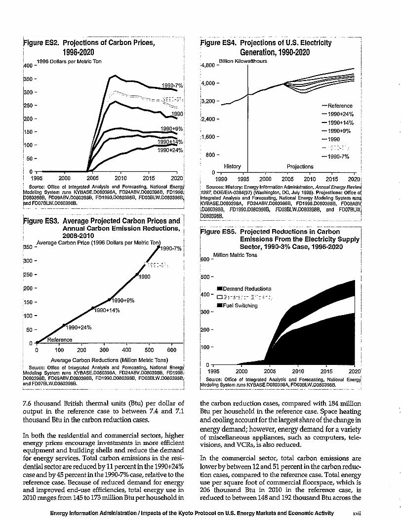
Figure ES2. Projections of Carbon Prices,1 1996-2020
1996 Dollars per Metric Ton
2010 2015 2020!
Source: Office of Integrated Analysis and Forecasting, National EnergyModeling System runs KYBASE.D080398A, FD24ABV.D080398B, FD1998JP080398B, FD09ABV.D080398B, FD1990.D080398B, FD03BLW.D080398BJand FD07BLW.D080398B. |
Figure ES3. Average Projected Carbon Prices andAnnual Carbon Emission Reductions,2008-2010
Average Carbon Price (1996 Dollars per Metric Ton)ic Ton)'1990-7% i
Reference
100 200 300 400 500 600
Average Carbon Reductions (Million Metric Tons) i
Source: Office of Integrated Analysis and Forecasting, National EnergyModeling System runs KYBASE.D080398A, FD24ABV.D080398B, FD1998i3080398B, FD09ABV.D080398B, FD1990.D080398B, FD03BLW.D080398B,and FD07BLW.D080398B. |
Figure ES4. Projections of U.S. ElectricityGeneration, 1990-2020
!4,800 -
4,000 -
Billion Kilowatthours
—Reference
— 1990+24%
—1990+14%
— 1990+9%
— 1990
8 0 0 - —1990-7%
0History Projections
1990 1995 2000 2005 2010 2015 2020Sources: History: Energy Information Administration, Annual Energy Revievi
1997, DOE/EIA-0384(97) (Washington. DC, July 1998). Projections: Office o{integrated Analysis and Forecasting, National Energy Modeling System runs;KYBASE.D080398A, FD24ABV.D080398B, FD1998.D080398B, FD09ABViD080398B, FD1990.D080398B, FD03BLW.D080398B, and FD07BLW,D080398B.
Figure ES5. Projected Reductions in CarbonEmissions From the Electricity SupplySector, 1990-3% Case, 1996-2020
MB 0 0 -
500-
Million Metric Tons
Demand Reductions
2000 2005 2010 2015 2020!
l_
! Source: Office of Integrated Analysis and Forecasting, National EnergyModeling System runs KYBASE.D080398A, FD03BLW.D080398B.
7.6 thousand British thermal units (Btu) per dollar ofoutput in the reference case to between 7.4 and 7.1thousand Btu in the carbon reduction cases.
In both the residential and commercial sectors, higherenergy prices encourage investments in more efficientequipment and building shells and reduce the demandfor energy services. Total carbon emissions in the resi-dential sector are reduced by 11 percent in the 1990+24%case and by 45 percent in the 1990-7% case, relative to thereference case. Because of reduced demand for energyand improved end-use efficiencies, total energy use in2010 ranges from 145 to 173 million Btu per household in
the carbon reduction cases, compared with 184 millionBtu per household in the reference case. Space heatingand cooling account for the largest share of the change inenergy demand; however, energy demand for a varietyof miscellaneous appliances, such as computers, tele-visions, and VCRs, is also reduced.
In the commercial sector, total carbon emissions arelower by between 12 and 51 percent in the carbon reduc-tion cases, compared to the reference case. Total energyuse per square foot of commercial floorspace, which is206 thousand Btu in 2010 in the reference case, isreduced to between 148 and 192 thousand Btu across the
Energy Information Administration / Impacts of the Kyoto Protocol on U.S. Energy Markets and Economic Activity

Figure ES6. Projected Reductions in CarbonEmissions by End-Use Sector Relativeto the Reference Case, 2010
160-
120-
8 0 -
4 0 -
Million Metric Tons
1990+24%
• Non-Elecinc•Electric
1990+9% 1990-3%
, Note: Electricity emissions are from the fuel used to generate elec-tricity and are attributed to the sectors relative to their shares of elec-tricity consumption. i
Source: Office of Integrated Analysis and Forecasting, National EnergyModeling System runs KYBASE.D080398A, FD24ABV.D080398B, FD09ABV:
cases. Similar to the residential sector, most of the reduc-tion occurs for space conditioning—heating, cooling,and ventilation; however, more efficient lighting andoffice equipment and reduced miscellaneous electricityuse—for example, for vending machines and telecom-munications equipment—also contribute to lowerenergy consumption.
The average price of gasoline in 2010 across the carbonreduction cases is between 11 and 53 percent higher thanthe projected reference case price. Carbon reductions inthe transportation sector in 2010 range from 2 to 16percent, primarily as the result of reduced travel and thepurchase of more efficient vehicles. The relatively lowcarbon reductions for transportation result from thecontinued dominance of petroleum, although someincrease in market share is projected for alternative-fuelvehicles. Improvements in average fuel efficiency areslowed by vehicle turnover rates. Although new carefficiency in 2010 improves from 30.6 miles per gallon inthe reference case to between 32.0 and 36.4 miles pergallon in the carbon reduction cases, total light-dutyfleet efficiency rises only from 20.5 miles per gallon tobetween 20.7 and 21.7 miles per gallon. The impact ofcarbon prices on the economy lowers light-duty vehicleand airline travel and freight requirements whileinducing some efficiency improvements.
Impacts by FuelIn order to achieve carbon emission reductions, the slateof energy fuels used in the United States is projected tochange from that in the reference case (Figure ES8).
Figure ES7. Projected Changes in AverageDelivered Prices for Energy Fuels inthe 1990+9% Case Relative to theReference Case, 1996-2020
400-
300-
200-
100-
1995
Percent
2000 2005 2010 2015 20201 Source: Office of Integrated Analysis and Forecasting, National EnergyModeling System runs KYBASE.D080398A and FD09ABV.D080398B.
Because of the higher relative carbon content of coal andpetroleum products, the use of both fuels is reduced,and there is a greater reliance on natural gas, renewableenergy, and nuclear power. Although the use of petro-leum declines relative to the reference case, it increasesslightly as a share because most petroleum is used in thetransportation sector, where fewer fuel substitutes areavailable.
Because of the high carbon content of coal, totaldomestic coal consumption is significantly reduced inthe carbon reduction cases, by between 18 and 77 per-cent relative to the reference case in 2010 (Figure ES9).Most of the reductions are for electricity generation,where coal is replaced by natural gas, renewable fuels,and nuclear power; however, demand for industrialsteam coal and metallurgical coal is also reducedbecause of a shift to natural gas in industrial boilers anda reduction in industrial output. Coal exports are alsolower in the carbon reduction cases, by between 21 and32 percent, due to lower demand for coal in the Annex Inations.
Although total U.S. coal production is reduced, theaverage minemouth coal price rises in the carbonreduction cases, by between 3 and 28 percent in 2010,because a larger share of production is from higher-costeastern coal mines that tend to serve the remainingmarkets. Production of western coal is further dis-couraged by the higher cost of fuels used for railtransportation and by reduced incentive for investmentin new mines, which are primarily in the West. Becauseof lower coal production, coal mine employment in 2010is projected to be 15 to 63 percent lower than in the

figure ES8. Projections of Fuel Shares of Total U.S. Energy Consumption, 2010Reference
(111.2 Quadrillion Btu) 39.4%
26.1%
1990+24%
(106.5 Quadrillion Btu) 40.2%
32.0%
1990-3%
a•••••
Oil
Natural GasCoal
Nuclear
RenewableOther
41.4%
7.9%
(93.9 Quadrillion Btu)7.1%1990+9%
(99.6 Quadrillion Btu) 1 1 - 8 %
Note: "Other" includes net electricity imports, methanol, and liquid hydrogen.Source: Office of Integrated Analysis and Forecasting, National Energy Modeling System runs KYBASE.D080398A, FD24ABV.D080398B, FD09ABV.D080398B, and
FD03BLW.D080398B.
reference case; however, employment in the energyindustry related to the production of natural gas andrenewable fuels is likely to increase.
Petroleum consumption is lower in all the carbon reduc-tion cases than in the reference case, by between 2 and 13percent (Figure ES10). Because most of the petroleum isused for transportation, between 68 and 82 percent ofthe total reduction is in the transportation sector, astravel and freight requirements are reduced and higher-efficiency vehicles are used. Because of lower petroleumdemand in the United States and in other developedcountries that are committed to reducing emissionsunder the Kyoto Protocol, world oil prices are lower by
between 4 and 16 percent in 2010, relative to the refer-ence case price of $20.77 per barrel. In 2010, net crude oiland petroleum product imports are lower by a range of 3to 22 percent relative to the reference case. Conse-quently, the dependency of the United States onimported petroleum is reduced from the reference caselevel of 59 percent to as little as 53 percent in 2010.
In 2010, natural gas consumption is higher than in thereference case, by a range of 2 to 12 percent across thecarbon reduction cases (Figure ES11). Increased use ofnatural gas in the generation sector is only partiallyoffset by reductions in the end-use sectors. Later inthe forecast period, continued growth in natural gas
Figure ES9. Projections of U.S. Coal Consumption,1970-2020
30-
25-
Quadrillion Btu
History Projections
0-r1970
Reference
1990+24%
1990+14%
1990+9%
19901990-3%1990-7%
Figure ES10. Projections of U.S. PetroleumConsumption, 1970-2020
,50-
4 5 -
;40-
;35-
130-
25 -
i20-
J 1 0 -i 5 -
Quadrillion Btu
History Projections
—Reference
—1990+24%
—1990+14%
— 1990+9%
—1990
— 1990-3%
—1990-7%
1980 1990 2000 2010 2020 1970 1980 1990 2000 2010 2020Sources: History: Energy Information Administration, Annual Energy Review
1997, DOE/EIA-0384(97) (Washington, DC, July 1998). Projections: Office ofIntegrated Analysis and Forecasting, National Energy Modeling System runs(<YBASE.D080398AI FD24ABV.D080398B, FD1998.D080398B, FD09ABV>D080398B, FD1990.D080398B, FD03BLW.D080398B, and FD07BLWJP080398B. j
| Sources: History: Energy Information Administration, Annual Energy Review\1997, DOE/EIA-0384(97) (Washington, DC, July 1998). Projections: Office o{Integrated Analysis and Forecasting, National Energy Modeling System runsKYBASE.D080398A, FD24ABV.D080398B, FD1998.D080398B, FD09ABV,'P080398B, FD1990.D080398B, FD03BLW.D080398B, and FD07BLW,1
P080398B.
Energy Information Administration / Impacts of the Kyoto Protocol on U.S. Energy Markets and Economic Activity

Figure ES11. Projections of U.S. Natural GasConsumption, 1970-2020
Quadrillion Btu
History Projections
5 -
—Reference
—1990+24%
— 1990+14%
— 1990+9%
—1990
—1990-7%
1970 1980 1990 2000 2010 2020!I Sources: History: Energy Information Administration, Annual Energy ReviewJ7997, DOE/EIA-0384(97) (Washington, DC, July 1998). Projections: Office ofIntegrated Analysis and Forecasting, National Energy Modeling System runsKYBASE.D080398A, FD24ABV.D080398B, FD1998.D080398B, FD09ABV.JD080398B, FD1990.D080398B, FD03BLW.D080398B, and FD07BLWJD080398B.
consumption for electricity generation is mitigated bythe increasing use of renewables and nuclear power,particularly in the more stringent carbon reductioncases. As a result, in 2020, natural gas use does not neces-sarily increase with higher levels of carbon reductions.As the result of higher demand, the average wellheadprice of natural gas in 2010 is higher in all the carboncases than in the reference case, by a range of 2 to 30 per-cent. Although meeting the levels of production thatmay be required will be a challenge for the industry, suf-ficient natural gas resources are available. The potentialincreases in both drilling and pipeline capacity arewithin levels achieved historically (or about to beachieved) and are not likely to be a constraint, givenappropriate incentives and planning.
Nuclear power, which produces no carbon emissions,increases with carbon reduction targets by between 8and 20 percent in 2010, relative to the reference case (Fig-ure ES12). Although no new nuclear plants are assumedto be built in the carbon reduction cases, extending thelifetimes of existing plants is projected to become moreeconomical with higher carbon prices. In the more strin-gent carbon reduction cases, most existing nuclearplants are life-extended through 2020, in contrast to thegradual retirement of approximately half of the nuclearplants projected in the reference case.
Consumption of renewable energy, which results in nonet carbon emissions, is projected to be significantlyhigher with carbon reduction targets (Figure ES13).Across the carbon reduction cases, renewable energyconsumption increases by between 2 and 16 percent in2010 and by between 9 and 70 percent in 2020. Most of
Figure ES12. Projections of U.S. Nuclear Energyi Consumption, 1970-2020
Quadrillion Btu
1990-7%
1990 "1990+9%1990+14%
1990+24%
Reference
2010 2020Sources: History: Energy Information Administration, Annual Energy Revlev\
\1997, DOE/EIA-0384(97) (Washington, DC, July 1998). Projections: Office ofIntegrated Analysis and Forecasting, National Energy Modeling System runs!KYBASE.D080398A, FD24ABV.D080398B, FD1998.D080398B, FD09ABVJD080398B, FD1990.D080398B, FD03BLW.D080398B, and FD07BLW.'D080398B.
figure ES13. Projections of U.S. RenewableEnergy Consumption, 1990-2020
1990+9%1990+14%1990+24%Reference
1990 1995 2000 2005 2010 2015 2020Sources: History: Energy Information Administration, Annual Energy Review,
\i997, DOE/E!A-0384(97) (Washington, DC, July 1998). Projections: Office ofjIntegrated Analysis and Forecasting, National Energy Modeling System runskYBASE.D080398A, FD24ABV.D080398B, FD1998.D080398B, FD09ABVJ'.D080398B, FD1990.D080398B, FD03BLW.D080398B, and FD07BLW^D080398B. !
this increase occurs in electricity generation, primarilywith additions to wind energy systems and an increasein the use of biomass (wood, switchgrass, and refuse). Inthe carbon reduction cases, the share of renewablegeneration is as much as 14 percent in 2010, comparedwith 10 percent in the reference case, increasing to ashigh as 22 percent in 2020, compared with 9 percentin the reference case. Because additional renewabletechnologies become available and economical later inthe forecast period, the share of renewable generationcontinues to increase through 2020.
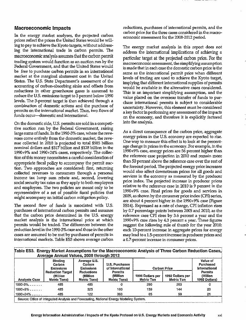
Macroeconomic ImpactsIn the energy market analyses, the projected carbonprices reflect the prices the United States would be will-ing to pay to achieve the Kyoto targets, without address-ing the international trade in carbon permits. Themacroeconomic analysis assumes that the carbon permittrading system would function as an auction run by theFederal Government, and that the United States wouldbe free to purchase carbon permits in an internationalmarket at the marginal abatement cost in the UnitedStates. The U.S. State Department's assessment of theaccounting of carbon-absorbing sinks and offsets fromreductions in other greenhouse gases is assumed toreduce the U.S. emissions target to 3 percent below 1990levels. The 3-percent target is then achieved through acombination of domestic actions and the purchase ofpermits on the international market. Thus, two flows offunds occur—domestic and international.
On the domestic side, U.S. permits are sold in a competi-tive auction run by the Federal Government, raisinglarge sums of funds. In the 1990-3% case, where the reve-nues come entirely from the domestic market, the reve-nue collected in 2010 is projected to total $585 billionnominal dollars and $317 billion and $128 billion in the1990+9% and 1990+24% cases, respectively. The collec-tion of this money necessitates a careful consideration ofappropriate fiscal policy to accompany the permit auc-tion. Two approaches are considered: first, returningcollected revenues to consumers through a personalincome tax lump sum rebate and, second, loweringsocial security tax rates as they apply to both employersand employees. The two policies are meant only to berepresentative of a set of possible fiscal policies thatmight accompany an initial carbon mitigation policy.
The second flow of funds is associated with U.S.purchases of international carbon permits and assumesthat the carbon price determined in the U.S. energymarket analysis is the international price at whichpermits would be traded. The differences between thereduction level in the 1990-3% case and those in the othercases are assumed to be met by purchases of permits ininternational markets. Table ES3 shows average carbon
reductions, purchases of international permits, and thecarbon price for the three cases considered in the macro-economic assessment for the 2008-2012 period.
The energy market analysis in this report does notaddress the international implications of achieving aparticular target at the projected carbon price. For themacroeconomic assessment, the simplifying assumptionis made that in each case the domestic carbon price is thesame as the international permit price when differentlevels of trading are used to achieve the Kyoto target,implying that different international supplies of permitswould be available in the alternative cases considered.This is an important simplifying assumption, and thevalue placed on the overseas transfer of funds to pur-chase international permits is subject to considerableuncertainty. However, this element must be considereda key factor in performing any assessment of the impactson the economy, and therefore it is explicitly factoredinto the analysis.
As a direct consequence of the carbon price, aggregateenergy prices in the U.S. economy are expected to rise.One way to measure this effect is to look at the percent-age change in prices in the economy. For example, in the1990+9% case, energy prices are 56 percent higher thanthe reference case projection in 2010 and remain morethan 50 percent above the reference case over the rest ofthe forecast period. The projected energy price increaseswould also affect downstream prices for all goods andservices in the economy as measured by the producerprice index. The projected increase in producer pricesrelative to the reference case in 2010 is 9 percent in the1990+9% case. Final prices for goods and services in2009, as shown by the consumer price index (CPI) series,are about 4 percent higher in the 1990+9% case (FigureES14). Expressed as a rate of change, CPI inflation risesby 0.7 percentage points between 2005 and 2010, as thereference case CPI rises by 3.6 percent a year and the1990+9% case rises by 4.3 percent a year. These figuressuggest the following rule of thumb for the year 2010:each 10-percent increase in aggregate prices for energymay lead to a 1.5-percent increase in producer prices anda 0.7-percent increase in consumer prices.
Table ES3. Energy Market Assumptions for the Macroeconomic Analysis of Three Carbon Reduction Cases,Average Annual Values, 2008 through 2012
Analysis Case
BindingCarbon
EmissionsReduction Target
(MillionMetric Tons)
1990-3% 485
1990+9% 485
1990+24% 485
Average U.S.Carbon
EmissionsReductions
(MillionMetric Tons)
485
325
122
U.S. Purchasesof International
Permits(Million
Metric Tons)0
160
363
Carbon Price
1996 Dollars perMetric Ton
1992 Dollars perMetric Ton
290 263159 14465 59
Value ofPurchased
InternationalPermits(Billion
1992 Dollars)0
23
21
Source: Office of Integrated Analysis and Forecasting, National Energy Modeling System.
Energy Information Administration / Impacts of the Kyoto Protocol on U.S. Energy Markets and Economic Activity
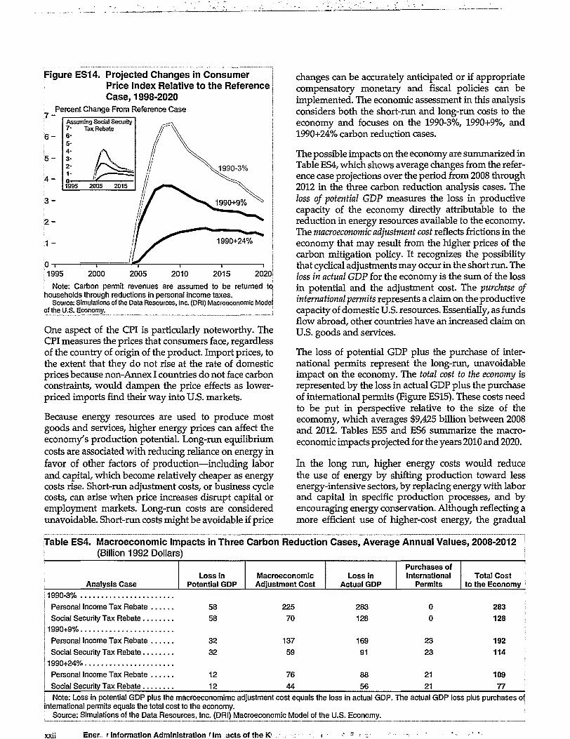
Figure ES14. Projected Changes in ConsumerPrice Index Relative to the ReferenceCase, 1998-2020
7-
6 -
5 -
4 -
3 -
Percent Change From Reference Case
1995 2000 2005 2010 2015 2020i
Note: Carbon permit revenues are assumed to be returned to;households through reductions in personal income taxes.
Source: Simulations of the Data Resources, Inc. (DRI) Macroeconomic Modelof the U.S. Economy.
One aspect of the CPI is particularly noteworthy. TheCPI measures the prices that consumers face, regardlessof the country of origin of the product. Import prices, tothe extent that they do not rise at the rate of domesticprices because non-Annex I countries do not face carbonconstraints, would dampen the price effects as lower-priced imports find their way into U.S. markets.
Because energy resources are used to produce mostgoods and services, higher energy prices can affect theeconomy's production potential. Long-run equilibriumcosts are associated with reducing reliance on energy infavor of other factors of production—including laborand capital, which become relatively cheaper as energycosts rise. Short-run adjustment costs, or business cyclecosts, can arise when price increases disrupt capital oremployment markets. Long-run costs are consideredunavoidable. Short-run costs might be avoidable if price
changes can be accurately anticipated or if appropriatecompensatory monetary and fiscal policies can beimplemented. The economic assessment in this analysisconsiders both the short-run and long-run costs to theeconomy and focuses on the 1990-3%, 1990+9%, and1990+24% carbon reduction cases.
The possible impacts on the economy are summarized inTable ES4, which shows average changes from the refer-ence case projections over the period from 2008 through2012 in the three carbon reduction analysis cases. Theloss of potential GDP measures the loss in productivecapacity of the economy directly attributable to thereduction in energy resources available to the economy.The macroeconomic adjustment cost reflects frictions in theeconomy that may result from the higher prices of thecarbon mitigation policy. It recognizes the possibilitythat cyclical adjustments may occur in the short run. Theloss in actual GDP for the economy is the sum of the lossin potential and the adjustment cost. The purchase ofinternational permits represents a claim on the productivecapacity of domestic U.S. resources. Essentially, as fundsflow abroad, other countries have an increased claim onU.S. goods and services.
The loss of potential GDP plus the purchase of inter-national permits represent the long-run, unavoidableimpact on the economy. The total cost to the economy isrepresented by the loss in actual GDP plus the purchaseof international permits (Figure ES15). These costs needto be put in perspective relative to the size of theecomomy, which averages $9,425 billion between 2008and 2012. Tables ES5 and ES6 summarize the macro-economic impacts projected for the years 2010 and 2020.
In the long run, higher energy costs would reducethe use of energy by shifting production toward lessenergy-intensive sectors, by replacing energy with laborand capital in specific production processes, and byencouraging energy conservation. Although reflecting amore efficient use of higher-cost energy, the gradual
Table ES4. Macroeconomic Impacts in Three(Billion 1992 Dollars)
Analysis CaseLoss in
Potential GDP
1990-3%
Personal Income Tax Rebate 58
Social Security Tax Rebate 58
1990+9%
Personal Income Tax Rebate 32
Social Security Tax Rebate 32
1990+24%
Personal Income Tax Rebate 12
Social Security Tax Rebate 12
Carbon Reductior
MacroeconomicAdjustment Cost
225
70
137
59
76
44
i Cases, Average Annual Values, 2008-2012
Loss inActual GDP
283
128
169
91
88
56Note: Loss in potential GDP plus the macroeconomimc adjustment cost equals the loss in actual GDP.'
international permits equals the total cost to the economy.Source: Simulations of the Data Resources, Inc. (DRI) Macroeconomic Model of the U.S. Economy.
Purchases ofInternational
Permits
0
0
23
23
21
21
Total Costto the Economy
283
128
192
114
109
77
Fhe actual GDP loss plus purchases ol
Ener. r Information Administration / Im acts of the K>

reduction in energy use would tend to lower the produc-tivity of other factors in the production process. Thederivation of the long-run equilibrium path of theeconomy can be characterized as representing the"potential" output of the economy when all resources—labor, capital, and energy—are fully employed. As such,potential GDP is equivalent to the full employment con-cept in other analyses that focus on long-run growthwhile abstracting from business cycle behavior. FigureES16 shows the losses in the potential economic output,as measured by potential GDP, for the three carbonreduction cases. The shapes of the three trajectoriesmirror the carbon price trajectories.
The ultimate impacts of carbon mitigation policies onthe economy will be determined by complex inter-actions between elements of aggregate supply anddemand, in conjunction with monetary and fiscal policydecisions. As such, cyclical impacts on the economyare bound to be characterized by uncertainty and con-troversy. However, raising the price of energy and
Figure ES15. Projected Annual Costs of CarbonReductions to the U.S. Economy,2008-2012
3 0 0 -
2 5 0 -
Billion 1992 Dollars •Purchase of Internationa! Permits j
•Loss in Potential GDP
•Macroeconomic Adjustment Cost ;
Assuming Personal IncomeTax Rebate
Assuming Social SecurityTax Rebate
1990-3% 1990+9% 1990+24%Source: Simulations of the Data Resources, Inc. (DRI) Macroeconomic Model
of the U.S. Economy. J
Table ES5. Projected Impacts on
Variable
Gross Domestic Product,
19962005
Reference
2005 and 2010
Refer-ence
1990+24%
1990+14%
20101990+9% 1990
1990-3%
1990-7%
| Potential GDP| (Billion 1992 Dollars) 6 ] 9 3 0
| (Percent Change From Reference Case) —| (Annual Growth Rate, 2005-2010, Percent) —
Actual GDP, Assuming Personal Income Tax Rebate| (Billion 1992 Dollars) 6 i g 2 8
j (Percent Change From Reference Case) '—i (Annual Growth Rate, 2005-2010, Percent) —
8,585 9,482 9,469 9,455 9,448 9,429 9,420— — -0.1 -0.3 -0.4 -0.6 -0.7— 2.0 2.0 1.9 1.9 1.9 1.9
8,525 9,429
— 2.0
| Actual GDP, Assuming Social Security Tax Rebate• (Billion 1992 Dollars); (Percent Change From Reference Case)j (Annual Growth Rate, 2005-2010, Percent)
6,928 8,525 9,429
2.0
9,333-1.01.8
9,369-0.61.9
9,268-1.71.7
9,337-1.01.8
9,241-2.01.6
9,326-1.11.8
9,137-3.11.4
9,291-1.51.7
9,102-3.51.3
9,410-0.81.9
9,032-4.21.2
9,281 9,247-1.6 -1.91.7 1.6
Source: Simulations of the Data Resources, Inc. (DRI) Macroeconomic Model of the U.S. Economy.
Table ES6. Projected Impacts on Gross Domestic Product, 2005 and 2020
Variable 19962005
Reference
2020
Refer-ence
1990+24%
1990+14%
1990+9% 1990
1990-3%
1990-7%
Potential GDP(Billion 1992 Dollars)(Percent Change From Reference Case)...(Annual Growth Rate, 2005-2020, Percent),
6,930 8,585 10,994 10,968 10,961 10,954 10,940 10,933 10,925— — -0.2 -0.3 -0.4 -0.5 -0.6 -0.6— 1.7 1.6 1.6 1.6 1.6 1.6 1.6
j Actual GDP, Assuming Personal Income Tax Rebate| (Billion 1992 Dollars) 6,928| (Percent Change From Reference Case) —(Annual Growth Rate, 2005-2020, Percent) —
8,525 10,865
1.6
Actual GDP, Assuming Social Security Tax Rebate(Billion 1992 Dollars)(Percent Change From Reference Case)(Annual Growth Rate, 2005-2020, Percent)
6,928 8,525 10,865
1.6
10,815-0.51.6
10,840-0.21.6
10,808-0.51.6
10,832-0.31.6
10,796-0.61.6
10,828-0.31.6
10,799-0.61.6
10,833-0.31.6
10,793-0.71.6
10,835-0.31.6
10,782-0.81.6
10,842-0.21.6
[ Source: Simulations of the Data Resources, Inc. (DRI) Macroeconomic Model of the U.S. Economy.
Energy Information Administration / Impacts of the Kyoto Protocol on U.S. Energy Markets and Economic Activity
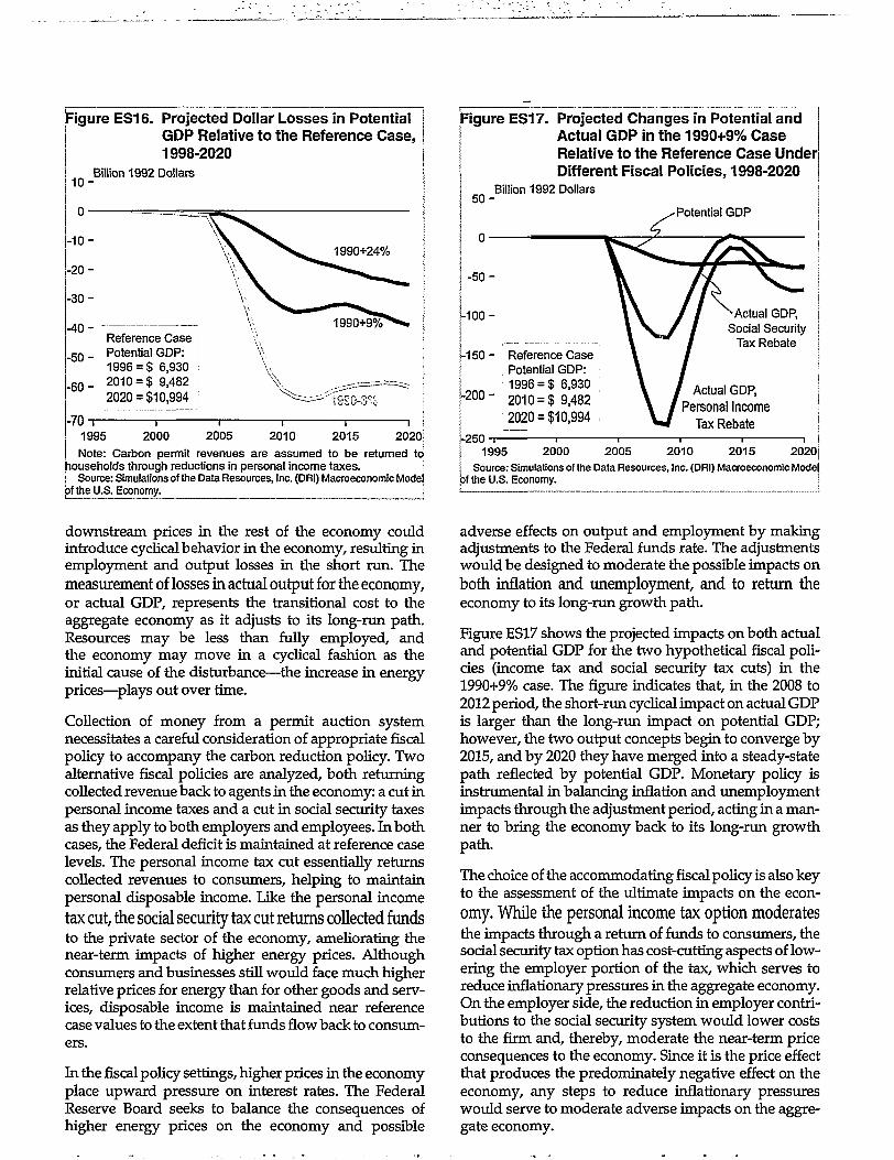
Figure ES16. Projected Dollar Losses in Potentialj GDP Relative to the Reference Case,I 1998-2020
1 0 -Billion 1992 Dollars
- 4 0 -Reference Case
50 - Potential GDP:j 1996 = $ 6,930
6 0 _ 2010 = $ 9,4822020 = $10,994
-701 r1890-3%
1995 2000 2005 2010 2015 2020
! Note: Carbon permit revenues are assumed to be returned tohouseholds through reductions in personal income taxes.j Source: Simulations of the Data Resources, Inc. (DRI) Macroeconomic Modelpf the U.S. Economy. I
Figure ES17. Projected Changes in Potential andActual GDP in the 1990+9% CaseRelative to the Reference Case UndeDifferent Fiscal Policies, 1998-2020
5 0 -Billion 1992 Dollars
- 5 0 -
100-
-150-
-200-
Reference CasePotential GDP:1996 = $ 6,9302010 = $ 9,4822020 = $10,994
-250-
Potential GDP
Actual GDP,Social Security
Tax Rebate
Actual GDP,' Personal Income
Tax Rebate
1995 2000 2005 2010 2015 2020
Source: Simulations of the Data Resources, Inc. (DRI) Macroeconomic Model3f the U.S. Economy.
downstream prices in the rest of the economy couldintroduce cyclical behavior in the economy, resulting inemployment and output losses in the short run. Themeasurement of losses in actual output for the economy,or actual GDP, represents the transitional cost to theaggregate economy as it adjusts to its long-run path.Resources may be less than fully employed, andthe economy may move in a cyclical fashion as theinitial cause of the disturbance—the increase in energyprices—plays out over time.
Collection of money from a permit auction systemnecessitates a careful consideration of appropriate fiscalpolicy to accompany the carbon reduction policy. Twoalternative fiscal policies are analyzed, both returningcollected revenue back to agents in the economy: a cut inpersonal income taxes and a cut in social security taxesas they apply to both employers and employees. In bothcases, the Federal deficit is maintained at reference caselevels. The personal income tax cut essentially returnscollected revenues to consumers, helping to maintainpersonal disposable income. Like the personal incometax cut, the social security tax cut returns collected fundsto the private sector of the economy, ameliorating thenear-term impacts of higher energy prices. Althoughconsumers and businesses still would face much higherrelative prices for energy than for other goods and serv-ices, disposable income is maintained near referencecase values to the extent that funds flow back to consum-ers.
In the fiscal policy settings, higher prices in the economyplace upward pressure on interest rates. The FederalReserve Board seeks to balance the consequences ofhigher energy prices on the economy and possible
adverse effects on output and employment by makingadjustments to the Federal funds rate. The adjustmentswould be designed to moderate the possible impacts onboth inflation and unemployment, and to return theeconomy to its long-run growth path.
Figure ES17 shows the projected impacts on both actualand potential GDP for the two hypothetical fiscal poli-cies (income tax and social security tax cuts) in the1990+9% case. The figure indicates that, in the 2008 to2012 period, the short-run cyclical impact on actual GDPis larger than the long-run impact on potential GDP;however, the two output concepts begin to converge by2015, and by 2020 they have merged into a steady-statepath reflected by potential GDP. Monetary policy isinstrumental in balancing inflation and unemploymentimpacts through the adjustment period, acting in a man-ner to bring the economy back to its long-run growthpath.
The choice of the accommodating fiscal policy is also keyto the assessment of the ultimate impacts on the econ-omy. While the personal income tax option moderatesthe impacts through a return of funds to consumers, thesocial security tax option has cost-cutting aspects of low-ering the employer portion of the tax, which serves toreduce inflationary pressures in the aggregate economy.On the employer side, the reduction in employer contri-butions to the social security system would lower coststo the firm and, thereby, moderate the near-term priceconsequences to the economy. Since it is the price effectthat produces the predominately negative effect on theeconomy, any steps to reduce inflationary pressureswould serve to moderate adverse impacts on the aggre-gate economy.
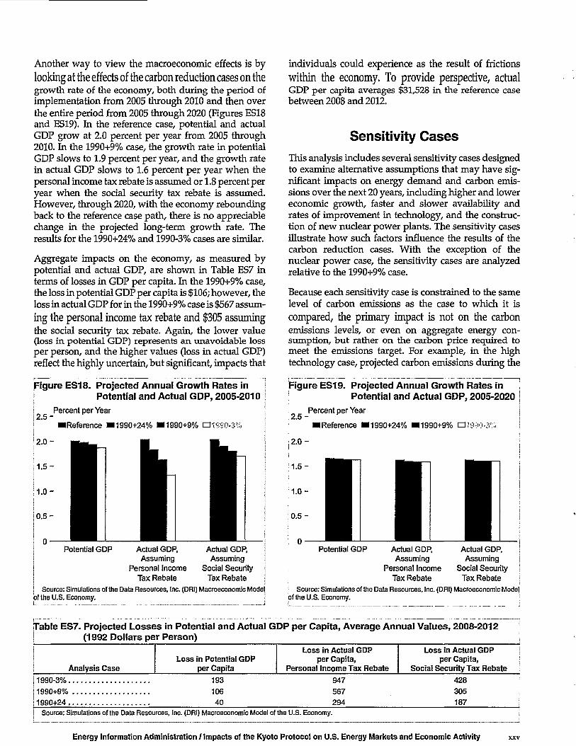
Another way to view the macroeconomic effects is bylooking at the effects of the carbon reduction cases on thegrowth rate of the economy, both during the period ofimplementation from 2005 through 2010 and then overthe entire period from 2005 through 2020 (Figures ES18and ES19). In the reference case, potential and actualGDP grow at 2.0 percent per year from 2005 through2010. In the 1990+9% case, the growth rate in potentialGDP slows to 1.9 percent per year, and the growth ratein actual GDP slows to 1.6 percent per year when thepersonal income tax rebate is assumed or 1.8 percent peryear when the social security tax rebate is assumed.However, through 2020, with the economy reboundingback to the reference case path, there is no appreciablechange in the projected long-term growth rate. Theresults for the 1990+24% and 1990-3% cases are similar.
Aggregate impacts on the economy, as measured bypotential and actual GDP, are shown in Table ES7 interms of losses in GDP per capita. In the 1990+9% case,the loss in potential GDP per capita is $106; however, theloss in actual GDP for in the 1990+9% case is $567 assum-ing the personal income tax rebate and $305 assumingthe social security tax rebate. Again, the lower value(loss in potential GDP) represents an unavoidable lossper person, and the higher values (loss in actual GDP)reflect the highly uncertain, but significant, impacts that
figure ES18. Projected Annual Growth Rates in! Potential and Actual GDP, 2005-2010
2.5-Percent per Year
•Reference •1990+24% •1990+9% IZ]1990-3%
mii 0 'Potential GDP Actual GDP, Actual GDP,
Assuming AssumingPersonal Income Social Security
Tax Rebate Tax Rebate| Source: Simulations of the Data Resources, Inc. (DRI) Macroeconomic Modelof the U.S. Economy. j
individuals could experience as the result of frictionswithin the economy. To provide perspective, actualGDP per capita averages $31,528 in the reference casebetween 2008 and 2012.
Sensitivity Cases
This analysis includes several sensitivity cases designedto examine alternative assumptions that may have sig-nificant impacts on energy demand and carbon emis-sions over the next 20 years, including higher and lowereconomic growth, faster and slower availability andrates of improvement in technology, and the construc-tion of new nuclear power plants. The sensitivity casesillustrate how such factors influence the results of thecarbon reduction cases. With the exception of thenuclear power case, the sensitivity cases are analyzedrelative to the 1990+9% case.
Because each sensitivity case is constrained to the samelevel of carbon emissions as the case to which it iscompared, the primary impact is not on the carbonemissions levels, or even on aggregate energy con-sumption, but rather on the carbon price required tomeet the emissions target. For example, in the hightechnology case, projected carbon emissions during the
Figure ES19. Projected Annual Growth Rates inI Potential and Actual GDP, 2005-2020
12.5-Percent per Year
IReference ^1990+24% ^1990+9% •S9iO-3r:,,
!2 .0 -
j 1.5 -
Potential GDP Actual GDP,Assuming
Personal IncomeTax Rebate
Actual GDP,Assuming
Social SecurityTax Rebate
; Source: Simulations of the Data Resources, Inc. (DRI) Macroeconomic Model'of the U.S. Economy. '
Table ES7. Projected Losses in Potential and Actual GDP per Capita, Average Annual Values, 2008-2012i (1992 Dollars per Person)
Analysis Case1990-3%1990+9%1990+24
Loss in Potential GDPper Capita
19310640
Loss in Actual GDPper Capita,
Personal Income Tax Rebate947567294
Loss in Actual GDPper Capita,
Social Security Tax Rebate428
305
187Source: Simulations of the Data Resources, Inc. (DRI) Macroeconomic Model of the U.S. Economy.
Energy Information Administration / Impacts of the Kyoto Protocol on U.S. Energy Markets and Economic Activity xxv
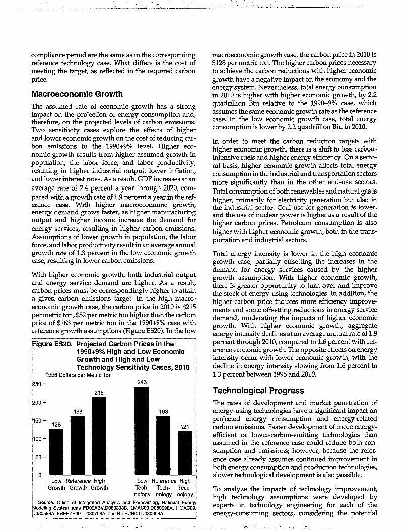
compliance period are the same as in the correspondingreference technology case. What differs is the cost ofmeeting the target, as reflected in the required carbonprice.
Macroeconomic GrowthThe assumed rate of economic growth has a strongimpact on the projection of energy consumption and,therefore, on the projected levels of carbon emissions.Two sensitivity cases explore the effects of higherand lower economic growth on the cost of reducing car-bon emissions to the 1990+9% level. Higher eco-nomic growth results from higher assumed growth inpopulation, the labor force, and labor productivity,resulting in higher industrial output, lower inflation,and lower interest rates. As a result, GDP increases at anaverage rate of 2.4 percent a year through 2020, com-pared with a growth rate of 1.9 percent a year in the ref-erence case. With higher macroeconomic growth,energy demand grows faster, as higher manufacturingoutput and higher income increase the demand forenergy services, resulting in higher carbon emissions.Assumptions of lower growth in population, the laborforce, and labor productivity result in an average annualgrowth rate of 1.3 percent in the low economic growthcase, resulting in lower carbon emissions.
With higher economic growth, both industrial outputand energy service demand are higher. As a result,carbon prices must be correspondingly higher to attaina given carbon emissions target. In the high macro-economic growth case, the carbon price in 2010 is $215per metric ton, $52 per metric ton higher than the carbonprice of $163 per metric ton in the 1990+9% case withreference growth assumptions (Figure ES20). In the low
Figure ES20. Projected Carbon Prices in the |1990+9% High and Low Economic jGrowth and High and Low jTechnology Sensitivity Cases, 2010 j
1996 Dollars per Metric Ton£50- 2 4 3
Low Reference HighGrowth Growth Growth
Low Reference HighTech- Tech- Tech-nology nology nology
Source: Office of Integrated Analysis and Forecasting, National EnergyModeling System runs FD09ABV.D080398B, LMAC09.D080698A, HMAC09JD080598A, FREEZE09. D080798A, and HITECH09.D080698A. j
macroeconomic growth case, the carbon price in 2010 is$128 per metric ton. The higher carbon prices necessaryto achieve the carbon reductions with higher economicgrowth have a negative impact on the economy and theenergy system. Nevertheless, total energy consumptionin 2010 is higher with higher economic growth, by 2.2quadrillion Btu relative to the 1990+9% case, whichassumes the same economic growth rate as the referencecase. In the low economic growth case, total energyconsumption is lower by 2.2 quadrillion Btu in 2010.
In order to meet the carbon reduction targets withhigher economic growth, there is a shift to less carbon-intensive fuels and higher energy efficiency. On a secto-ral basis, higher economic growth affects total energyconsumption in the industrial and transportation sectorsmore significantly than in the other end-use sectors.Total consumption of both renewables and natural gas ishigher, primarily for electricity generation but also inthe industrial sector. Coal use for generation is lower,and the use of nuclear power is higher as a result of thehigher carbon prices. Petroleum consumption is alsohigher with higher economic growth, both in the trans-portation and industrial sectors.
Total energy intensity is lower in the high economicgrowth case, partially offsetting the increases in thedemand for energy services caused by the highergrowth assumption. With higher economic growth,there is greater opportunity to turn over and improvethe stock of energy-using technologies. In addition, thehigher carbon price induces more efficiency improve-ments and some offsetting reductions in energy servicedemand, moderating the impacts of higher economicgrowth. With higher economic growth, aggregateenergy intensity declines at an average annual rate of 1.9percent through 2010, compared to 1.6 percent with ref-erence economic growth. The opposite effects on energyintensity occur with lower economic growth, with thedecline in energy intensity slowing from 1.6 percent to1.3 percent between 1996 and 2010.
Technological ProgressThe rates of development and market penetration ofenergy-using technologies have a significant impact onprojected energy consumption and energy-relatedcarbon emissions. Faster development of more energy-efficient or lower-carbon-emitting technologies thanassumed in the reference case could reduce both con-sumption and emissions; however, because the refer-ence case already assumes continued improvement inboth energy consumption and production technologies,slower technological development is also possible.
To analyze the impacts of technology improvement,high technology assumptions were developed byexperts in technology engineering for each of theenergy-consuming sectors, considering the potential

impacts of increased research and development formore advanced technologies. The revised assumptionsincluded earlier years of introduction, lower costs,higher maximum market potential, and higher efficien-cies than assumed in the reference case.9 Also, thissensitivity case assumed the availability of carbonsequestration technology for coal- and natural-gas-firedpower plants, which would remove carbon dioxide andstore it in underground aquifers; however, the technol-ogy is uneconomical relative to other technologiesbecause of its high operating and storage costs.
These technological improvements were developedunder the assumption of increased research and devel-opment, and they are distinct from the more rapid adop-tion of advanced technologies that occurs with higherenergy prices in the carbon reduction cases. It is possiblethat further technology improvements could occurbeyond those in the high technology sensitivity case if avery aggressive research and development effort wereestablished. The low technology sensitivity caseassumes that all future equipment choices are madefrom the end-use and generation equipment available in1998, with new building shell and industrial plant effi-ciencies frozen at 1998 levels. Comparing this sensitivitycase to a case with reference technology assumptionsdemonstrates the importance of technology improve-ment in the reference case.
Because faster technology development makes ad-vanced energy-efficient and low-carbon technologiesmore economically attractive, the carbon prices requiredto meet carbon reduction levels are significantlyreduced. Conversely, slower technology improvementrequires higher carbon prices (Figure ES20). With hightechnology assumptions, the carbon price in 2010 is $121per metric ton, $42 per metric ton lower than the carbonprice of $163 per metric ton in the 1990+9% case with thereference technology assumptions. With the low tech-nology assumptions, the carbon price increases to $243per metric ton in 2010.
In the high technology sensitivity case, total energyconsumption in 2010 is lower by 2.1 quadrillion Btu, orabout 2 percent, than in the 1990+9% case with referencetechnology. Delivered energy consumption in both theindustrial and transportation sectors is lower asefficiency improvements in industrial processes andmost transportation modes outweigh the countervailingeffects of lower energy prices. In the residential andcommercial sectors, the effect of lower energy pricesbalances the effect of advanced technology, andconsumption levels are at or near those in the referencetechnology (1990+9%) case. In the generation sector, coaluse for generation is 40 percent higher than with
reference technology assumptions, due to efficiencyimprovements and the lower carbon price.
In the low technology sensitivity case, the conversetrends prevail. In 2010, total energy consumption ishigher by 1.5 quadrillion Btu than in the 1990+9% casewith reference technology assumptions. Deliveredenergy consumption is higher in the industrial andtransportation sectors and lower in the residential andcommercial sectors, suggesting that industry and trans-portation are more sensitive to technology changes thanto price changes, and the residential and commercialsectors are more sensitive to price changes. With thehigher carbon prices in the low technology case, coal useis further reduced in the generation sector, and morenatural gas, nuclear power, and renewables are used tomeet the carbon reduction targets.
Nuclear PowerIn the reference case, nuclear electricity generationdeclines significantly because 52 percent of the totalnuclear capacity available in 1996 is assumed to beretired by 2020. A number of units are retired before theend of their 40-year operating licenses, as suggested byindustry announcements and analysis of the age andoperating costs of the units. In the carbon reductioncases, life extension of the plants can occur if it iseconomical; and there is an increasing incentive to investin nuclear plant refurbishment with higher carbonprices. However, these cases do not allow the construc-tion of new nuclear power plants, given continuing highcapital investment costs and institutional constraintsassociated with nuclear power. A nuclear power sensi-tivity case examines the impact of allowing new plantsto be constructed. Because nuclear plants still are noteconomically competitive with fossil and renewableplants in the 1990+9% case, the nuclear power sensitivitycase was analyzed against the 1990-3% case. In additionto allowing new nuclear plants, the higher costsassumed in the reference case for the first few advancednuclear plants were reduced in this sensitivity.
Relative to the 1990-3% case, 1 gigawatt of new nuclearcapacity is added by 2010 in the nuclear power sensitiv-ity case, and 41 gigawatts, representing about 68 newplants of 600 megawatts each, are added by 2020. Withmost of the impact from the new nuclear plants comingafter the commitment period of 2008 through 2012, thereis little impact on carbon prices in 2010. By 2020, how-ever, carbon prices are $199 per metric ton with theassumption of new nuclear plants, as compared with$240 per metric ton in the 1990-3% case with the refer-ence nuclear assumptions. In 2010, total energy con-sumption is about the same in this sensitivity case as in
9The design of the high technology sensitivity case differs from the high technology cases in AEO98, which generally did not include ananalysis of improvements for specific technologies.
Energy Information Administration / Impacts of the Kyoto Protocol on U.S. Energy Markets and Economic Activity xxvii
the 1990-3% case, but in 2020 it is about 1.8 quadrillionBtu higher. Somewhat lower energy prices inducehigher consumption in all sectors, and the availability ofmore carbon-free nuclear generation allows the carbonreduction target to be met with higher end-use con-sumption.
Uncertainties in the Analysis
The reference case projections in both AEO98 and thisanalysis represent business-as-usual forecasts, givenknown trends in technology and demographics, currentlaws and regulations, and the specific methodologiesand assumptions used by EIA. Because EIA does notinclude future legislative and regulatory changes in itsreference case projections, the projections provide apolicy-neutral baseline against which the impacts of pol-icy initiatives can be analyzed.
Results from any model or analysis are highly uncertain.By their nature, energy models are simplified represen-tations of complex energy markets. The results of anyanalysis are highly dependent on the specific data,assumptions, behavioral characteristics, methodologies,and model structures included. In addition, many of thefactors that influence the future development of energymarkets are highly uncertain, including weather, politi-cal and economic disruptions, technology development,and policy initiatives. Recognizing these uncertainties,EIA has attempted in this study to isolate and analyzethe most important factors affecting future carbon emis-sions and carbon prices. The results of the various casesand sensitivities should be considered as relativechanges to the comparative baseline cases.
In addition to the uncertainties concerning the finalinterpretation and implementation of the Kyoto Proto-col, specific actions that might be taken to reduce green-house gas emissions in the United States have not beenformulated. Actions taken by other Annex I countries toreduce emissions, future growth in worldwide energyconsumption and emissions, and the opportunities forreducing emissions through joint implementation and
the CDM are unknown, and they are likely to haveimportant impacts on the international trade of carbonpermits and the carbon permit price. This analysisassumes that auctioned permits will constrain carbonemissions and raise the price of fossil fuels, with reve-nues from the auction recycled to consumers eitherthrough personal income tax or social security taxrebates. Alternative carbon reduction programs and fis-cal policies would be likely to change the cost of carbonreduction from the costs in this analysis. The timing ofcarbon reduction programs and the amount of adjust-ment time allowed could also be important in determin-ing costs.
Future technology development also cannot be knownwith certainty and may have a significant effect on thecost of achieving carbon reductions. The technology sen-sitivity cases in this analysis explore some of the poten-tial impacts, but even the high technology sensitivitydoes not include possible breakthrough or speculativetechnologies. On title other hand, even the reference casetechnology assumptions include continued develop-ment of more energy-efficient and renewable technolo-gies, which serve to mitigate the costs of carbonreduction. Those technology improvements are likely,but not certain.
Finally, consumer response to carbon initiatives isuncertain. Because energy price changes that haveoccurred in the past may not provide sufficient evidenceabout the reaction of consumers to sustained highenergy prices, changes in demand as a result of thehigher carbon fees cannot be projected with confidence.In addition to price-induced changes, consumers mightalso respond to climate change initiatives and a nationalcommitment to reduce emissions by adopting moreenergy-efficient or renewable technologies sooner thanexpected. Finally, public acceptance of large-scalerenewable technologies or the continuation of nuclearpower—both of which make important contributions tothe achievement of the carbon emissions reductions atthe costs projected in this analysis—cannot be knownwith certainty.
1. Scope and Methodology of the Study
Background
The Greenhouse Gas EffectThe greenhouse effect is a natural process by whichsome of the radiant heat from the Sun is captured in thelower atmosphere of the Earth, thus maintaining thetemperature of the Earth's surface. The gases that helpcapture the heat, called "greenhouse gases," includewater vapor, carbon dioxide, methane, nitrous oxide,and a variety of manufactured chemicals. Some areemitted from natural sources; others are anthropogenic,resulting from human activities.
Over the past several decades, rising concentrations ofgreenhouse gases have been detected in the Earth'satmosphere. Although there is not universal agreementwithin the scientific community on the impacts ofincreasing concentrations of greenhouse gases, it hasbeen theorized that they may lead to an increase in theaverage temperature of the Earth's surface. To date, ithas been difficult to note such an increase conclusivelybecause of the differences in temperature around theEarth and throughout the year, and because of the diffi-culty of distinguishing permanent temperature changesfrom the normal fluctuations of the Earth's climate. Inaddition, there is not universal agreement among scien-tists and climatologists on the potential impacts of anincrease in the average temperature of the Earth,although it has been hypothesized that it could lead to avariety of changes in the global climate, sea level, agri-cultural patterns, and ecosystems that could be, on net,detrimental.
The most recent report of the Intergovernmental Panelon Climate Change (IPCC) concluded that: "Our abilityto quantify the human influence on global climate is cur-rently limited because the expected signal is still emerg-ing from the noise of natural variability, and becausethere are uncertainties in key factors. These include the
magnitudes and patterns of long-term variability andthe time-evolving pattern of forcing by, and response to,changes in concentrations of greenhouse gases and aero-sols, and land surface changes. Nevertheless, the bal-ance of evidence suggests that there is a discernablehuman influence on global climate."1
U.S. Greenhouse Gas EmissionsIn 1990, total greenhouse gas emissions in the UnitedStates were 1,618 million metric tons carbon equivalent,2
according to 1997 estimates published by the EnergyInformation Administration (EIA).3 Of this total, 1,346million metric tons, or 83 percent, was due to carbonemissions from the combustion of energy fuels—thefocus of this report. By 1996, total U.S. greenhouse gasemissions had risen to 1,753 million metric tons carbonequivalent, including 1,463 million metric tons of carbonemissions from energy combustion. EIA's Annual EnergyOutlook 1998 (AEO98y projects that energy-related car-bon emissions will reach 1,577 million metric tons in2000,17 percent above the 1990 level. Projected emis-sions continue to rise at an average annual rate of 1.5percent a year from 1996 to 2010, reaching 1,803 millionmetric tons of carbon emissions in 2010, 34 percentabove the 1990 level. Because energy-related carbonemissions are a large portion of total greenhouse gasemissions, any efforts to reduce greenhouse gas emis-sions will likely have a significant impact on the energysector; however, as discussed later, there are a numberof factors outside the domestic energy market that alsoaffect emissions levels.
To put U.S. emissions in a global perspective, the UnitedStates produced about 24 percent of the worldwideenergy-related carbon emissions in 1996, which totaled6.6 billion metric tons, as noted in EIA's InternationalEnergy Outlook 1998 (IEO98).5 Although continuedincreases in carbon emissions are expected for theUnited States and other industrialized countries, much
1Intergovernmental Panel on Climate Change, Climate Change 1995: The Science of Climate Change (Cambridge, UK: Cambridge UniversityPress, 1996).
2Greenhouse gases differ in their impacts on global temperatures. For comparison of emissions from the various gases, they are oftenweighted by global warming potential (GWP), established by the Intergovernmental Panel on Climate"Change, which is a measure of theimpact of each gas on global warming relative to that of carbon dioxide, which is defined as having a GWP equal to 1.
3Energy Information Administration, Emissions of Greenhouse Gases in the United States 1996, DOE/EIA-0573(96) (Washington, DC, Octo-ber 1997).
4Energy Information Administration, Annual Energy Outlook 1998, DOE/EIA-0383(98) (Washington, DC, December 1997).5Energy Information Administration, International Energy Outlook 1998, DOE/EIA-0484(98) (Washington, DC, April 1998).
Energy Information Administration / Impacts of the Kyoto Protocol on U.S. Energy Markets and Economic Activity 1
more rapid increases are projected for the developingcountries of Asia, the Middle East, Africa, and Centraland South America. As a result, global carbon emissionsfrom energy use are expected to increase at an averageannual rate of 2.4 percent from 1996 through 2010, reach-ing 8.3 billion metric tons, to which the United Stateswould contribute about 22 percent.
The Framework Convention onClimate ChangeAs a result of increasing warnings by members of the cli-matological and scientific community about the possibleharmful effects of rising greenhouse gas concentrations,the IPCC was established by the World MeteorologicalOrganization and the United Nations EnvironmentProgramme in 1988 to assess the available scientific,technical, and socioeconomic information in the field ofclimate change. A series of international conferencesfollowed, and in 1990 the United Nations established theIntergovernmental Negotiating Committee for a Frame-work Convention on Climate Change. After a seriesof negotiating sessions, the text of the Framework Con-vention on Climate Change was adopted at the UnitedNations on May 9,1992, and opened for signature at Riode Janeiro on June 4.
The objective of the Framework Convention was to " . . .achieve . . . stabilization of the greenhouse gas concen-trations in the atmosphere at a level that would preventdangerous anthropogenic interference with the climatesystem." The signatories agreed to "formulate, imple-ment, . . . and . . . update . . . programmes containingmeasures to mitigate climate change by addressinganthropogenic emissions by sources and removals bysinks" and to prepare periodic emissions inventories,promote development and diffusion of technologies foremissions control, and cooperate in adaptation. In addi-tion, the developed country signatories agreed to "adoptnational policies and take corresponding measures onthe mitigation of climate change" and to "communicate.. . detailed information on its policies and measures . . .with the aim of returning individually or jointly to their1990 levels these anthropogenic emissions of carbondioxide and other greenhouse gases." The Conventionexcludes chlorofluorocarbons (CFCs) and hydrochloro-fluorocarbons (HCFCs), greenhouse gases that aredeemed to cause damage to the Earth's stratosphericozone and are controlled by the 1987 Montreal Protocolon Substances that Deplete the Ozone Layer.
The Framework Convention established the Conferenceof the Parties to "review the implementation of the Con-vention and . . . make, within its mandate, the decisionsnecessary to promote the effective implementation." In1995, the first Conference of the Parties met in Berlin andissued the Berlin mandate, an agreement to "begin aprocess to enable it to take appropriate action for the pe-riod beyond 2000." The second Conference of the Par-ties, held in Geneva in July 1996, called for negotiationson quantified limitations and reductions of greenhousegas emissions and policies and measures for the thirdConference of the Parties in Kyoto, Japan, in December1997.
The Climate Change Action PlanResponding to the Framework Convention, on April 21,1993, President Clinton called upon the United States tostabilize greenhouse gas emissions by 2000 at 1990 lev-els. Specific steps to achieve U.S. stabilization were enu-merated in the Climate Change Action Plan (CCAP),6
published in October 1993, which consists of a series of44 actions to reduce greenhouse gas emissions. Theactions include voluntary programs, industry partner-ships, government incentives, research and develop-ment, regulatory programs including energy efficiencystandards, and forestry actions. Greenhouse gasesaffected by these actions include carbon dioxide, meth-ane, nitrous oxide, hydrofluorocarbons (HFCs), and per-fluorocarbons (PFCs). At the time CCAP was developed,the Administration estimated that the actions it enumer-ated would reduce total net emissions7 of these green-house gases in the United States to 1990 levels by 2000.
In addition to the climate-related actions of CCAP, theEnergy Policy Act of 1992 (EPACT), Section 1605(a), pro-vided for an annual inventory of U.S. greenhouse gasemissions, which is contained in the EIA publicationseries, Emissions of Greenhouse Gases in the United States.8
Also, Section 1605(b) of EPACT established the Vol-untary Reporting Program, permitting corporations,government agencies, households, and voluntaryorganizations to report to EIA on actions that havereduced or avoided emissions of greenhouse gases. Theresults of the Voluntary Reporting Program are reportedannually by EIA, most recently in Mitigating GreenhouseGas Emissions: Voluntary Reporting,9 which reports 1995activities. Entities providing data to the VoluntaryReporting Program include some participants ingovernment-sponsored voluntary programs, such as the
President William J. Clinton and Vice President Albert Gore, Jr., The Climate Change Action Plan (Washington, DC, October 1993).7Carbon dioxide is absorbed by growing vegetation and soils. Defining the total impacts of CCAP as net reductions accounts for the
increased sequestration of carbon dioxide as a result of the forestry and land-use actions in the program.8Energy Information Administration, Emissions of Greenhouse Gases in the United States 1996, DOE/EIA-0573(96) (Washington, DC, Octo-
ber 1997).9Energy Information Administration, Mitigating Greenhouse Gas Emissions: Voluntary Reporting, DOE/EIA-0608(96) (Washington, DC,
October 1997).
Climate Wise and Climate Challenge programs, whichare cosponsored by the U.S. Environmental ProtectionAgency and the U.S. Department of Energy to fosterreductions in greenhouse gas emissions by industry andelectricity generators. Voluntary activities for 1996 and1997 will be available in the fall of 1998.
The Kyoto ProtocolPrior to the third Conference of the Parties, at the June26, 1997, Earth Summit+5 Conference at the UnitedNations, President Clinton pledged U.S. support forbinding emissions targets and announced three initia-tives: a pledge of $1 billion over 5 years by the UnitedStates for the development of more energy-efficient andalternative energy technologies in developing countries;
the strengthening of environmental guidelines for U.S.companies investing overseas; and a partnership withprivate industry to install solar panels on 1 million roof-tops in the United States by 2010.
On October 22,1997, President Clinton proposed thatdeveloped countries should stabilize emissions at 1990levels between 2008 and 2012, with reductions below1990 levels in the following 5-year period. He also indi-cated his support for joint implementation projects andinternational emissions trading and declared that par-ticipation by developing countries was necessary for theUnited States to assume binding obligations. At thesame time, the President announced additional initia-tives to address greenhouse gas emissions: a $5 billionprogram of tax incentives and research and develop-ment spending for energy-efficient and lower-carbontechnologies; the establishment of an emissions tradingsystem with credit for early reductions; the restructuringof the electricity industry; and reductions of emissionsfrom Federal sources. Funding for the program wasincreased to $6.3 billion in the Administration's 1999budget request.
Representatives from more than 160 countries met inKyoto on December 1 through 11, 1997. The resultingKyoto Protocol established binding emissions targets fordeveloped nations, relative to their emissions levels in1990, for an overall reduction of about 5 percent.10
The individual targets for the Annex I countries11 rangefrom an 8-percent reduction for the European Union(EU) (or its individual member states) to a 10-percentincrease allowed for Iceland. Australia and Norway alsoare allowed increases of 8 and 1 percent, respectively,
while New Zealand, the Russian Federation, and theUkraine are held to their 1990 levels. Other EasternEuropean countries undergoing transition to marketeconomies have reduction targets of between 5 and 8percent. The reduction targets for Canada and Japan are6 percent and, for the United States, 7 percent. Althoughatmospheric concentrations of greenhouse gases ulti-mately have the potential to affect the global climate, theProtocol establishes targets in terms of annual emissions.
The greenhouse gases included in the targets are carbondioxide, methane, nitrous oxide, hydrofluorocarbons,perfluorocarbons, and sulfur hexafluoride.12 For the lat-ter three gases, individual nations have the option ofusing 1995 as the base year from which to achieve reduc-tions, instead of 1990. The aggregate target is establishedusing the carbon dioxide equivalent of each of the green-house gases. Other greenhouse gases are not limited bythe Protocol, although CFCs and HCFCs are controlledby the Montreal Protocol. This analysis focuses on car-bon emissions from the combustion of energy fuels,which constituted 83 percent of all U.S. greenhouse gasemissions in 1990. Carbon dioxide emissions fromsources other than energy use are not included in theanalysis, nor are emissions of the five other gases cov-ered by the Kyoto Protocol; however, reductions inthose gases may lessen the required reductions inenergy-related carbon emissions, as discussed below.
The established targets must be achieved over the pe-riod 2008 to 2012, the first commitment period.Essentially, each country can average its emissions overthat 5-year period to establish compliance, smoothingout short-term fluctuations that might result fromeconomic cycles or extreme weather patterns. Eachcountry must have made demonstrable progress by2005. No targets are established for the period after 2012,although lower targets may be set by future Conferencesof the Parties.
Sources of emissions include fuel combustion, fugitiveemissions from fuels, industrial processes, solvents,agriculture, and waste management and disposal. TheProtocol does not prescribe specific actions to be takenbut lists a number of potential actions, including energyefficiency improvements, enhancement of carbon-absorbing sinks, such as forests and other vegetation,research and development of sequestration technolo-gies, phasing out of fiscal incentives and subsidies that
10The text of the Kyoto Protocol is available at web site www.unfccc.de.11 Australia, Austria, Belgium, Bulgaria, Canada, Croatia, Czech Republic, Denmark, Estonia, European Community, Finland, France,
Germany, Greece, Hungary, Iceland, Ireland, Italy, Japan, Latvia, Liechtenstein, Lithuania, Luxembourg, Monaco, Netherlands, New Zea-land, Norway, Poland, Portugal, Romania, Russian Federation, Slovakia, Slovenia, Spain, Sweden, Switzerland, Ukraine, United Kingdomof Great Britain and Northern Ireland, and United States of America. Turkey and Belarus are Annex I nations that have not ratified the Con-vention and did not commit to quantifiable emissions targets.
12Hydrofluorocarbons are a non-ozone-depleting substitute for CFCs; perfluorocarbons are byproducts of aluminum production andare also used in semiconductor manufacturing; and sulfur hexafluoride is used as an insulator in electrical equipment and in semiconductormanufacturing.
Energy Information Administration / Impacts of the Kyoto Protocol on U.S. Energy Markets and Economic Activity
may inhibit the goal of emissions reductions, and reduc-tion of methane emissions in waste management and inenergy production, distribution, and transportation.
Several provisions of the Protocol allow for some flexi-bility in meeting the emissions targets. Net changes inemissions by direct anthropogenic land-use changesand forestry activities will also be used in meeting thecommitment; however, these are limited to afforesta-tion, reforestation, and deforestation since 1990. Emis-sions trading among the Annex I countries is permitted.No rules for trading are established, however, and theConference of the Parties is required to establish princi-ples, rules, and guidelines for trading at a future date.Joint implementation projects are also allowed amongthe Annex I countries, whereby a nation could take emis-sions credits for projects that reduce emissions orenhance sinks in other countries. It is specifically indi-cated that trading and joint implementation are supple-mental to domestic actions.
The Protocol also establishes a Clean DevelopmentMechanism (CDM), under which Annex I countries cantake emissions credits for projects that reduce emissionsin non-Annex I countries, provided that the projects leadto measurable, long-term benefits. Reductions fromsuch projects undertaken from 2000 until the first com-mitment period can be used to assist compliance in thecommitment period. This provision calls for the estab-lishment of an executive board to oversee the projects. Inaddition, an unspecified share of the proceeds from theproject activities must be used to cover administrativeexpenses and to assist with adaptation those countriesthat are particularly vulnerable to climate change.
Banking—the carrying over of unused allowances fromone commitment period to the next—is allowed; how-ever, the borrowing of emissions allowances from afuture commitment period is not permitted. Under theProtocol, Annex I countries, such as the nations ofthe European Union (EU), may create a bubble orumbrella to meet the total commitment of all themember nations. In a bubble, countries agree to meet thetotal commitment jointly by allocating a share to eachmember. In an umbrella arrangement, the total reduc-tion of all member nations is met collectively throughthe trading of emissions rights. There is potential inter-est in the United States in entering into an umbrella trad-ing arrangement.
Non-Annex I countries have no targets under the Proto-col, although it reaffirms the commitments of the Frame-work Convention by all parties to formulate andimplement climate change mitigation and adaptationprograms and to promote the development and diffu-sion of environmentally sound technologies andprocesses. Developing countries can voluntarily enterinto the Protocol by full amendment of the Protocol.
The Protocol became open for signature on March 16,1998, for a 1-year period. Under its provisions, it entersinto force 90 days following acceptance of at least 55Parties, including Annex I countries accounting for atleast 55 percent of the total 1990 carbon dioxide emis-sions from Annex I nations. Signature by the UnitedStates would need to be followed by Senate advise andconsent to ratification.
There are a number of uncertainties and issues to beresolved at future Conferences of the Parties. As indi-cated in the Protocol, rules and guidelines for theaccounting of emissions and sinks from activities relatedto agriculture, land use, and forestry activities must bedeveloped. The specific guidelines may have a signifi-cant impact on the level of reductions from other sourcesthat a country must undertake. This issue was directedto the IPCC by subsequent climate change talks in Bonnin June 1998. In addition, rules and guidelines must beestablished for emissions trading, joint implementationprojects, and the CDM.
Other issues covered in the Protocol but deferred to sub-sequent sessions include flexibility for Annex I countriesundergoing transition to market economies, commit-ments for subsequent periods, climate change adapta-tion actions, sanctions for failure to meet commitments,guidelines for the reporting and review of emissions andsinks, and international cooperation in education,research and development, and technology transfer.
Emissions TradingEven before the Kyoto Protocol, many analyses of theimpacts of greenhouse gas emissions reductions havefavored emissions trading programs, including jointimplementation programs, as a means of achievingemissions reductions. In the United States, the Clean AirAct Amendments of 1990 (CAAA90) established a trad-ing program for emissions of sulfur dioxide (SO2) byelectricity generators in order to reduce emissions tofixed specified levels. Permits issued to electricity gen-erators allow them to emit up to a specified level of SO2,with the total number of issued permits equal to thenational limit on emissions. Generators may reduceemissions by using lower-sulfur coals, installing scrub-bers, or increasing the utilization of cleaner-generatingplants. Generators that reduce emissions below theirallowed levels can sell excess emissions permits, whichcan be purchased by other generators for whom it ismore cost-effective to purchase permits at the prevailingmarket price than to reduce emissions. Emissions per-mits can also be banked for future use. Compared withtraditional control programs that mandate specific com-pliance options or require uniform reductions, this SO2
trading program is credited with reducing the overallcost of compliance by allowing reductions to be made inthe most cost-effective manner.

Unlike SO2, carbon emissions are primarily an interna-tional, rather than domestic, issue. In theory, a similartrading scheme for carbon emissions could be formu-lated either internationally or within individual coun-tries to achieve fixed emissions levels. Indeed, the KyotoProtocol provides for international emissions tradingbut defers the determination of specific guidelines andrules for establishing an open trading market and man-aging the international flow of funds for the purchase ofpermits. Additional complexities may arise in establish-ing baseline projections against which to monitor andverify net emissions reductions, particularly with regardto the CDM.
Even within the United States, carbon emissions tradingmay be more complicated than the current SO2 tradingplan for several reasons. The largest sources of SO2 are asmall number of large coal-burning generation plants.This makes it .relatively easy to monitor their fuel useand emissions and to build and maintain an allowancetrading system to ensure compliance. In contrast, thereare a large number of entities that emit carbon, includinghouseholds, commercial establishments, industrialfacilities, automobiles, trucks, airplanes, ships, andfossil-fired generating stations. The development andoperation of a monitoring and trading system for carbonemissions would thus be much more complicated. Inaddition, there were technologies available to reduceSO2 emissions at generation plants at the time the allow-ance trading program was initiated, and switching tolow-sulfur coal was an option. Although research isongoing, there are no readily available pre- or post-combustion technologies for removing carbon fromfossil fuels (although the high technology sensitivitycase included in this analysis assumes that carbonsequestration technologies will become available forelectricity generators). Therefore, the options for carbonreduction are limited to fuel switching to lower-carbonor carbon-free fuels, efficiency improvements, and re-ductions in energy demand.
Methodology of the AnalysisIn March 1998, the U.S. House of Representatives Com-mittee on Science requested that the EIA perform ananalysis of the Kyoto Protocol, focusing on the impactsof the Protocol on U.S. energy prices, energy use, and theeconomy in the 2008 to 2012 time frame for a number ofemissions targets. (See letters of request in Appendix D.)The request specified that the analysis use the same ref-erence case assumptions as in AEO98 unless changes inthe assumptions could be justified on the basis of theProtocol—that is, there should be no changes in assump-tions regarding policy, regulatory actions, or fundingof energy or environmental programs, including theenergy-related provisions of the Administration's reve-nue proposals of February 1998.
Each target in the analysis was to be achieved on averagebetween 2008 and 2012, phasing in beginning in 2005and stabilizing at the target level after 2012, althoughtargets beyond 2012 have not yet been established andmay in fact be more stringent. The Committee indicatedthat no new nuclear plants should be allowed, althougheconomical life extensions of nuclear plants should bepermitted. Construction of new nuclear plants, varia-tions in economic growth, and different assumptionsconcerning technology characteristics were all to be ana-lyzed as sensitivities to the target cases.
Numerous studies have been conducted on the topic ofreducing greenhouse gas emissions. They can be clus-tered into several broad categories. One group of studiesare cost-benefit analyses, which seek to establish an opti-mal level of either emissions reductions or emissionsprices with a goal of balancing the costs and benefits ofemissions reductions, explicitly accounting for the miti-gation of damage as a result of emissions controls. A sec-ond category of studies address the cost-effectiveness ofalternative paths for emissions reductions. Assuming alevel of global concentrations of greenhouse gases, theseanalyses derive an optimal timing strategy for the impo-sition of emissions controls.
Other studies are more narrowly focused on the costs ofachieving specific emissions reductions or on theimpacts of policies and technology on emissions levels.Before the Conference of the Parties in Kyoto, analysesexamined the costs of emissions targets under a varietyof assumptions about the possible level and timing ofthe targets. Since the Conference, analyses have focusedon the levels and timing specified in the Kyoto Protocoland studied the costs of achieving those levels under arange of assumptions about the international provisionsand other flexibility measures in the Protocol. Some ofthose analyses are included in the comparison of resultsin Chapter 7. This EIA analysis is among this final cate-gory of studies, with more detail on U.S. energy marketsand the economy than other analyses but not addressingthe potential benefits of emissions reductions, optimaltiming, or international trade.
The Protocol includes a number of international provi-sions—including international emissions trading, jointimplementation projects, and the CDM—that mayreduce the cost of compliance. Because EIA cannot fullyaddress these aspects of the Protocol at this time, theanalysis focuses on domestic impacts and includes arange of cases with different levels of energy-relatedcarbon emissions. Although any impact on the globalclimate will likely be caused by atmospheric concentra-tions of greenhouse gases, the targets in the Kyoto Proto-col are in terms of annual emissions. This analysisaddresses the annual emissions targets as specified inthe Protocol.
Energy Information Administration / Impacts of the Kyoto Protocol on U.S. Energy Markets and Economic Activity

The National Energy Modeling SystemAt the request of the Committee, this analysis uses thesame basic assumptions and methodologies that wereused for AEO98. The projections in AEO98 were devel-oped using the National Energy Modeling System(NEMS), an energy-economy modeling system of U.S.energy markets, which is designed, implemented, andmaintained by EIA.13 The production, imports, conver-sion, consumption, and prices of energy are projectedfor each year through 2020, subject to assumptions onmacroeconomic and financial factors, world energymarkets, resource availability and costs, behavioral andtechnological choice criteria, costs and performancecharacteristics of energy technologies, and demograph-ics. NEMS is a fully integrated framework, capturing theinteractions of energy supply, demand, and pricesacross all fuels and all sectors of U.S. energy markets.
Reference case projections are developed annually usingNEMS and published in the Annual Energy Outlook(AEO). NEMS is also used to analyze the effects of exist-ing and proposed laws, regulations, and standardsrelated to energy production and use; the impacts ofnew and advanced energy technologies; the savingsfrom higher energy efficiency; the impacts of energy taxpolicy on the U.S. economy and energy system; and theimpacts of environmental policies, such as the CAAA90and regulations on alternative and reformulated fuels.Special analyses of these and other topics are performedat the request of the U.S. Congress, other offices in theU.S. Department of Energy, and other government agen-cies. Because NEMS provides annual projections, it iswell suited to represent the transitional effects of pro-posed energy policy and regulation.
Within NEMS, four end-use demand modules representenergy consumption in the residential, commercial,industrial, and transportation sectors, subject to fuelprices, macroeconomic factors, and the characteristics ofenergy-using technologies in those sectors. The fuel sup-ply and conversion modules represent the domestic pro-duction, imports, transportation, and conversionprocesses to meet the domestic and export demand forcoal, petroleum products, natural gas, and electricity,accounting for resource base characteristics, industryinfrastructure and technology, and world market condi-tions. The modules of NEMS interact to solve for the eco-nomic supply and demand balance for each fuel.
In order to capture regional differences in energy con-sumption patterns and resource availability, NEMS is aregional model. The end-use demand for energy is rep-resented for each of the nine Census divisions. The sup-ply and conversion modules use the North American
Electric Reliability Council regions and subregions forelectricity generation; aggregations of the PetroleumAdministration for Defense Districts for refineries; andproduction regions specific to oil, natural gas, and coalsupply and distribution.
NEMS incorporates interactions between the energysystem and the economy and between domestic andworld oil markets. Key macroeconomic variables,including the gross domestic product (GDP), disposablepersonal income, industrial output, housing starts,employment, and interest rates, drive energy consump-tion and investment decisions. In turn, changes inenergy prices and energy activity affect economic activ-ity, a feedback captured within NEMS. Also, an interna-tional energy module in NEMS represents world oilprices, production, and demand and the interactionsbetween the domestic and world oil markets. Within thismodule, world oil prices and supplies respond tochanges in U.S. demand and production.
Technology Representation in NEMSA key feature of NEMS is the representation of technol-ogy and technology improvement over time. The resi-dential, commercial, transportation, electricitygeneration, and refining sectors of NEMS includeexplicit treatments of individual technologies and theircharacteristics, such as initial cost, operating cost, date ofcommercial availability, efficiency, and other character-istics specific to the sector. In addition, for new generat-ing technologies, the electricity sector accounts fortechnological optimism in the capital costs of first-of-a-kind plants and for a decline in the costs as experiencewith the technologies is gained both domestically andinternationally. In each of these sectors, equipmentchoices are made for individual technologies as newequipment is needed to meet growing demand forenergy services or to replace retired equipment. In addi-tion, in the electricity generation sector, fossil-fired andnuclear generating units can be retired before the end oftheir useful lives if it is more economical to bring on a re-placement unit than to continue to operate the existingunit.
In the other sectors—industrial, oil and gas supply, andcoal supply—the treatment of technologies is somewhatmore limited due to limitations on the availability ofdata for individual technologies. In the industrial sector,technology improvement for the major processing stepsof the energy-intensive industries is represented bytechnology possibility curves of efficiency improve-ments over time. In the oil and gas supply sector, tech-nology progress for exploration and productionactivities is represented by trend-based improvement in
13See Energy Information Administration, The National Energy Modeling System: An Overview 1998, DOE/EIA-0581(98) (Washington, DC,February 1998), for a summary description. Detailed documentation is available through the National Energy Information Center at202/586-8800 or on the EIA web site at www.eia.doe.gov.
Ener. r Information Administration / Ini acts of the Ki Ao Protocol on U.S. Ener: r Markets and Economic ActivL

finding rates, success rates, costs, and the size of theresource base. Productivity improvements over timerepresent technological progress in coal production.
Because of the detailed representation of capital stockvintaging and technology characteristics, NEMS cap-tures the most significant factors that influence the turn-over of energy-using and producing equipment and thechoice of new technologies. New, more advanced tech-nologies for buildings and equipment are generallycharacterized by the technology costs, performance, andavailability, existing standards, and energy prices.Equipment that does not meet efficiency standards is notavailable as a choice.
The relative costs of purchasing and operating differenttypes of equipment are factored into consumer choices,which are represented by elasticities and discount ratesderived from the analysis of available data. Within theresidential sector, for example, housing stocks are calcu-lated by region and housing type, using aggregate hous-ing starts from the macroeconomic forecast andassumed retirement rates. Stocks of energy-using equip-ment are also tracked, reflecting equipment retirement,replacements, and new housing starts. Choices for newequipment and efficiency levels for new houses areinfluenced by the characteristics of available technology,existing standards, energy prices, and consumer prefer-ences as reflected in past decisions. In the end-use sec-tors, all technology choices are based on the assumptionthat future energy prices will remain at the same level asthe prices for the year in which the decision is beingmade, this being the most likely representation of howcustomer decisions are made. However, in the genera-tion and refining sectors, which are cost minimizers,capacity expansion decisions include foresight of futureenergy prices and demand.
In all sectors, technology improvement occurs even in areference case because new, more efficient technologywill be adopted as demand for energy services increasesand existing buildings and equipment are retired. Thecharacteristics of the technologies include initial dates ofcommercial availability of more advanced technologiesas well as changes in efficiency and cost that areassumed to occur in the future. Higher energy pricesmay accelerate the adoption of more efficient technolo-gies. Past improvements in energy efficiency haveresulted in part from efficiency standards that areincluded in the analysis; future efficiency standardsassumed are those approved standards with specifiedefficiency levels.
The detailed characterization of energy consumptionpatterns and technology decisions in NEMS allows foran explicit representation of the introduction of newenergy-using equipment and the improvement of the
capital stock. Because longer-term forecasting modelstypically are not annual models, they tend not to capturethe gradual transition of energy markets, including thecapital stock vintaging and turnover, as NEMS does. Inaddition, because of the longer time horizon, longer-term models tend to have less detailed representationsof energy markets.
Although prices play a role in consumers' decisions on
energy-consuming equipment, there are other factorsthat come into play. Consumers tend to make decisionsbased on a number of personal preferences and lifestylechoices, in which energy prices may be only a part of thedecisionmaking process. Preferences for larger televi-sions or higher horsepower vehicles are examples of fac-tors that may outweigh energy costs. As anotherexample, in the residential sector, home rental instead ofpurchase and frequent moving tend to lower the incen-tive to invest in more energy-efficient equipment. Infor-mation also has a major role in consumer decisions andwill likely continue to do so in the adoption of new, moreadvanced technologies. Particularly when a more effi-cient or alternatively fueled technology carries a signifi-cantly higher cost or has different operationalcharacteristics than more conventional technologies,information on the benefits of the new technology willbe key to its adoption and penetration. Ultimately, thesuccess of a given technology will depend not on thebehavior of the marginal consumer, who may be par-ticularly cost-conscious or innovative, but on the behav-ior of the average consumer, whose decision rests on anumber of considerations.
Technology improvements, even when adopted in themarket, may not necessarily lead to reductions in energydemand. In the transportation sector, for example, theuse of more advanced technologies that could improvevehicle efficiency has been offset by increasing demandfor larger and higher horsepower vehicles. To the extentthat energy prices are a factor in consumer decisions,efficiency improvements may also increase energydemand. Efficiency gains may lower the cost of drivingor operating other equipment, perhaps encouragingmore travel, larger homes, and purchases of more equip-ment and increasing the demand for energy services.
New or tightened efficiency standards could also reducethe demand for energy, but stock turnover would stilllimit the speed of penetration. Standards have also beensuggested to encourage the use of renewable fuels forelectricity generation, such as those in the proposedElectric System Public Benefits Protection Act of 1997,the proposed Electric Consumers Protection Act of 1997,and the Administration's proposed ComprehensiveElectricity Competition Act; however, proposed andpossible future standards, legislation, and programs arenot included in the analysis.
Energy Information Administration / Impacts of the Kyoto Protocol on U.S. Energy Markets and Economic Activity

The Annual Energy Outlook 1998
At the request of the Committee on Science, this study ofthe impacts of the Kyoto Protocol is based on the refer-ence case assumptions of AEO98. In accordance with therequirement that the reference case EIA projections bepolicy-neutral, the AEO98 projections assume that allFederal, State, and local law, regulations, policies, andstandards in effect as of July 1,1997, remain unchangedthrough 2020. Potential impacts of pending or proposedlegislation, proposed standards, or sections of existinglegislation for which funds had not been appropriatedare not included in the projections. In general, theAEO98 projections were prepared using the- most cur-rent data available as of July 31,1997.
The AEO98 projections assume continued growth in theU.S. economy, with GDP growing at an average annualrate of 1.9 percent through 2020. Additional key factorsunderlying the projections are the assumptions con-cerning world oil markets. Continued technologicalimprovement in the production of oil and the expansionof production capability worldwide hold the increase inthe real, inflation-adjusted world oil price to an averagegrowth rate of 0.4 percent a year. Domestically, withtechnological advances in the exploration and produc-tion of natural gas, the average annual growth in theaverage wellhead price is projected to be 0.5 percenteven with rapid growth in the demand for natural gas.The average price of coal declines throughout the projec-tion period due to increasing productivity in coal pro-duction and the expansion of production from lower-cost western sources.
AEO98 represents the ongoing restructuring of the elec-tricity industry by assuming lower operating, mainte-nance, and administrative costs, as noted in the trends ofrecent data; early retirements of higher-cost coal-firedand nuclear power plants; and lower capital costs andefficiency improvements for coal- and natural-gas-firedgeneration technologies. Additional assumptionsinclude a revised financial structure that features ahigher cost of capital in competitive markets. Specificrestructuring plans are included for those regions thathave announced plans. California, New York, and NewEngland are assumed to begin competitive pricing in1998 with stranded cost recovery phased out by 2008.The provisions of the California legislation for strandedcost recovery and price caps are incorporated. Withthese assumptions and declining coal prices, electricityprices decline at an average annual rate of 1 percent inthe AEO98 projections.
Electricity generation from nuclear power declines sig-nificantly in the projections. About 20 percent of thenuclear capacity available in 1996 is assumed to beretired by 2010, with no new plants constructed. It isassumed that nuclear units would be retired as early as10 years before the expiration of their operating licenses,
based on utility announcements and on analysis of theage and operating costs of the units. To offset the declineof nuclear power and to meet the growth of electricitydemand, coal and natural gas generation expand in theprojections, particularly the gas technologies. The finan-cial assumptions for restructuring weigh against morecapital-intensive projects, such as coal and baseloadrenewable technologies.
With decreases or moderate increases in the prices ofenergy and continued economic growth, total energyconsumption in AEO98 increases by 1 percent a year onaverage through 2020. Consumption in all end-use sec-tors grows in the projections; however, demand in thetransportation sector increases most rapidly, reflectingincreased travel and slow improvement in the efficiencyof vehicles. Total energy intensity, measured as energyuse per dollar of GDP, declines in the projections at anaverage annual rate of 0.9 percent. This rate is considera-bly less than the 2.3-percent decline in energy intensityexperienced between 1970 and 1986 when rapid priceincreases and a shift to less energy-intensive industriesled to rapid energy intensity improvements. On aver-age, energy intensity has been flat between 1986 and1996. The projected improvement still reflects continuedimprovements in energy efficiency that partially offsetincreases in the demand for energy services.
As noted earlier, projected carbon emissions fromenergy combustion in AEO98 reach 1,803 million metrictons in 2010,34 percent above the 1990 level of 1,346 mil-lion metric tons, rising to 1,956 million metric tons in2020. Total emissions are projected to increase at anaverage annual rate of 1.5 percent between 1996 and2010 in the reference case, and per capita emissions alsoincrease at an average annual rate of 0.7 percent duringthat period, as continued economic growth and moder-ate price increases encourage growth in energy servicesand energy consumption. Between 2010 and 2020, effi-ciency improvements tend to offset continued growth inthe demand for energy services, and per capita emis-sions nearly flatten. During that period, total emissionsincrease at an average rate of 0.8 percent a year. Over theentire projection period, the slow growth of renewabletechnologies and the decline of electricity generationfrom nuclear power plants also contribute to the growthof emissions.
Projections of carbon emissions in AEO98 include EIA'sanalysis of the impacts of CCAP for the 31 of the 44CCAP actions that relate to carbon dioxide emissionsfrom energy combustion. The analysis does not accountfor the remaining actions related to non-energy pro-grams, gases other than carbon dioxide, or forestry andland use. The analysis of CCAP represents EIA's esti-mate of the effects of incorporating assumptions con-cerning behavioral change as a result of CCAP and doesnot result in the reductions estimated by the developers
of CCAP. The initial estimates of the impacts of theCCAP actions by the Administration projected stabiliza-tion of net greenhouse gas emissions in 2000 at 1990 lev-els; however, a more recent review and update of CCAPsignificantly reduces the expected impact.14 In AEO98,carbon emissions in 2010 are reduced by about 36 mil-lion metric tons as a result of CCAP, compared with themore recent estimate by the sponsors of about 95 millionmetric tons for the energy-related actions in CCAP. Dif-ferences between the CCAP impacts estimated by EIAand by the program sponsors are due primarily to differ-ences in the estimated impacts of voluntary programs;some estimates by the sponsors that include ongoingtrends that would occur even in the absence of CCAP;and regulatory actions included by the sponsors but notincluded by EIA because they are not yet enacted orfinalized.
The Annual Energy Outlook 1995 (AEO95)15 was the firstAEO to include the impacts of CCAP in the projections.Even then, the goal of stabilizing carbon emissions in2000 at 1990 levels seemed unlikely. AEO95 projectedthat energy-related carbon emissions would reach 1,471million metric tons in 2000, a level nearly reached in 1996when emissions were 1,463 million metric tons. Eachsubsequent AEO has raised the estimate of carbon emis-sions, primarily because of lower price projections thatencourage energy use and reduce the penetration ofrenewable sources of energy.
There are several reasons that the target specified byCCAP for 2000 is unlikely to be realized. First, U.S. eco-nomic growth has been slightly higher than assumed atthe time the CCAP programs were formulated. Second,energy prices have increased at a more moderate ratethan initially assumed in the early 1990s. Both these fac-tors have contributed to higher growth in energy con-sumption than earlier assumed, leading to higheremissions levels. Third, the funding for a number of theCCAP programs is lower than initially requested.Finally, some voluntary programs have proven lesseffective than initially estimated by the Administration.
Carbon Reduction CasesThe Kyoto Protocol specifies that the U.S. target for totalgreenhouse gas emissions in the first commitment peri-od will be 7 percent below the level of emissions in 1990.This analysis focuses on the carbon dioxide emissionsfrom the use of energy, which constituted 83 percent oftotal U.S. greenhouse emissions in 1996 (1,463 millionmetric tons of energy-related carbon emissions in the
total greenhouse gas emissions of 1,753 million metrictons carbon equivalent).
The specific reduction in energy-related carbon emis-sions that will be required is highly dependent on anumber of factors outside the domestic energy sector.Programs to reduce emissions of the other five green-house gases covered by the Protocol may decrease therequirement for reductions in carbon dioxide emissions.Similarly, forestry, agriculture, and land use programsmay also offset some carbon dioxide emissions; how-ever, the rules to account for agriculture and forestryemissions and sinks have yet to be developed and aresubject to considerable uncertainty. According to a factsheet prepared by the U.S. Department of State on Janu-ary 15, 1998, discussing the Kyoto negotiations, themethod of accounting for sinks and the flexibility to use1995 as the base year for the synthetic greenhouse gassesmay mean that the reduction would be no more man 3percent below 1990 levels, based on the Administra-tion's estimates.16 Similar estimates were cited by Dr.Janet Yellen, Chair, Council of Economic Advisers, inher testimony before the House Committee on Com-merce, Energy and Power Subcommittee, on March 4,1998.17 Finally, because this analysis does not fully rep-resent international energy markets and other activities,the potential role of international emissions trading andthe CDM in alleviating U.S. reductions of carbon dioxideis not directly represented in the analysis. Even thoseanalyses that do include international trade must makeassumptions about the activities, because the develop-ment of guidelines and mechanisms has been deferred.
The success of programs to reduce greenhouse gases atrelatively low costs may depend on the success of inter-national trade of carbon permits, joint implementationprojects, and the CDM. Some analyses of greenhouse gasreductions that have low costs of compliance assumethat a number of relatively low-cost carbon permits willbe available from Annex I countries with less expensiveopportunities to reduce emissions. Based on EIA'sanalysis in IEO98, there may be 165 million metric tonsof carbon permits available from the Annex I countriesin the former Soviet Union in 2010, because of the eco-nomic decline of those countries in the 1990s, and addi-tional permits may be available as a result of carbonreduction projects. The total estimate of such opportuni-ties is highly uncertain, however, and it is also unclearwhether those countries would choose to sell availablepermits immediately or bank them for later use as theireconomies and populations grow. The potential transac-tion costs of international trading are also unknown.
14U.S. Department of State, Office of Global Change, Climate Action Report, Department of State Publication 10496 (Washington, DC, July1997).
15Energy Information Administration, Annual Energy Outlook 1995, DOE/EIA-0383(95) (Washington, DC, January 1995).16See web site www.state.gov/www/global/oes/fs_kyoto_climate_980115.html.^See web site www.house.gov/commerce/database.htm.
Energy Information Administration / Impacts of the Kyoto Protocol on U.S. Energy Markets and Economic Activity 9

The role of developing countries is another area ofuncertainty for international activities. In July 1997, theSenate unanimously passed the Byrd-Hagel resolution,sponsored by Senators Robert Byrd of West Virginia andChuck Hagel of Nebraska, resolving "that the UnitedStates should not be a signatory to any protocol to, orother agreement regarding, the United Nations Frame-work Convention on Climate Change . . . which wouldmandate new commitments to limit or reduce green-house gas emissions for the Annex I Parties, unless theprotocol or other agreement also mandates new specificscheduled commitments . . . for Developing CountryParties within the same compliance period or wouldresult in serious harm to the economy of the UnitedStates."1 President Clinton has declared on severaloccasions that he will not submit the Protocol for ratifi-cation without pledges of meaningful participation bydeveloping countries. While participation by develop-ing countries may be key to the acceptance of the Proto-col, development of specific guidelines and rules for theinternational programs has been deferred, including themeans to establish baseline projections and to monitorand verify emissions reductions.
There is also a possibility that investments to reduce car-bon emissions in developing countries could be limited.First, such bilateral ventures may be viewed as substi-tutes for or additions to foreign aid, a political concern toboth the United States and developing countries. Also, itis possible that the continuing discussions about theimplementation of the Protocol will raise the topic oftrade limits—restrictions on the amount of reductionsthat any one country can satisfy through internationalprograms. The Protocol states that such activities are tobe supplemental to domestic actions. In the views ofsome countries, there is a potential problem with certainnations undertaking little internal action.
Because the potential impacts of forestry and agricul-tural sinks, offsets from other greenhouse gases, interna-tional trading, and other international activities areuncertain, a single target for the required reductions inenergy-related carbon emissions in the United Statescannot be developed at present. This analysis includes anumber of cases, as requested by the Committee, assum-ing different levels of reductions in energy-related car-bon emissions, in order to develop the energy andeconomic impacts of achieving those reductions. Byestablishing this range of carbon reductions, the analysisallows others to perform their own analyses of theimpacts of sinks, offsets, and international programs,derive their own targets for energy-related carbon emis-sions, and use one of the EIA target cases to assess theenergy and economic impacts of the carbon reductionsin that case.
In addition to a reference case, six targets for reductionsin energy-related carbon emissions are considered.
• Reference Case (33 Percent Above 1990 Levels).This case represents the reference projections ofenergy markets and carbon emissions without anyenforced reductions and is presented as a compari-son for the energy market impacts in the reductioncases. Although this reference case is based on thereference case from AEO98, as specified by the Com-mittee, there are small differences between this caseand AEO98. Some modifications were made in orderto permit additional flexibility in NEMS in responseto higher energy prices or to include certain analysespreviously done offline directly within the modelingframework, such as nuclear plant life extension andgenerating plant retirements. Also, some assump-tions were modified to reflect more recent assess-ments of technological improvements and costs.Significant changes to NEMS and its assumptionsrelative to AEO98 axe noted in Appendix A. As aresult of these modifications, the projections of car-bon emissions in the reference case for this analysisare slightly lower than those in the AEO98 referencecase—1,791 million metric tons in 2010 comparedwith 1,803 million metric tons. The carbon emissionsprojections in the reference case, as well as in all thecarbon reduction cases, include EIA's estimate of theimpacts of CCAP.
• 24 Percent Above 1990 Levels (1990+24%). This caseassumes that carbon emissions can increase to anaverage of 1,670 million metric tons in the commit-ment period 2008 to 2012,24 percent above the 1990levels, but 122 million metric tons below the average
. emissions in the reference case during that period.
• 14 Percent Above 1990 Levels (1990+14%). This caseassumes that carbon emissions in the commitmentperiod average 1,539 million metric tons, which isapproximately the level estimated for 1998 in AEO98and is 14 percent above 1990 levels. This requires theaverage annual carbon emissions between 2008 and2012 to be reduced by 253 million metric tons.
• 9 Percent Above 1990 Levels (1990+9%). This caseassumes that energy-related carbon emissions canreach an average of 1,467 million metric tons in thecommitment period, 9 percent above 1990 levels, anaverage reduction of 325 million metric tons from thereference case projection.
•Stabilization at 1990 Levels (1990). This caseassumes that carbon emissions are stabilizedapproximately at the 1990 level of 1,346 million met-ric tons, averaging 1,345 million metric tons during
18The discussion about the resolution can be accessed in the Congressional Record of July 25,1997, from web site www.access.gpo.gov/su_docs/aces/acesl50.html.

the commitment period, a reduction of 447 millionmetric tons from the reference case.
• 3 Percent Below 1990 Levels (1990-3%). This caseassumes that energy-related carbon emissions arereduced to an average of 1,307 million metric tons inthe commitment period. A reduction of 485 millionmetric tons from the reference case level is required.
• 7 Percent Below 1990 Levels (1990-7%). In this case,energy-related carbon emissions are reduced to anaverage of 1,250 million metric tons in the commit-ment period, a reduction of 542 million metric tonsfrom the reference case projection. This case essen-tially assumes that energy-related carbon emissionsmust meet the 7-percent target in the Kyoto Protocolwith no net offsets from sinks, other greenhousegases, or international activities.
Reductions in both the 1990-3% and 1990-7% caseswould likely come from domestic actions only. Thereductions in the other carbon reduction cases implysome international trade in carbon permits, CDM activ-ity, or joint implementation projects, but this analysisdoes not address the shares that might result from inter-national and domestic actions.
In each of the carbon reduction cases, the target isachieved on average for each of the years in the firstcommitment period, 2008 through 2012, in accordancewith the Kyoto Protocol. The Protocol provides the flexi-bility for the target to be achieved on average over the 5-year commitment period, to accommodate short-termfluctuations that might occur, such as severe weather orunanticipated economic growth. Because the Protocoldoes not specify any targets beyond the first commit-ment period, the target is assumed to hold constant from2013 through 2020, the end of the NEMS forecast hori-zon. This assumption may be optimistic in that the possi-bility of further reductions has been advocated.
The target is assumed to be phased in over a 3-year peri-od, beginning in 2005; that is, one-fourth of the reductionis imposed in 2005, one-half in 2006, and three-fourths in2007. This analytical simplification allows energy mar-kets to begin adjustments to meet the reduction targetsin the absence of complete foresight, although a longeror delayed phase-in may lower the adjustment cost.Phase-in is also consistent with the requirement in theProtocol that countries achieve demonstrable progresstoward the reductions by 2005; however, reductionsprior to the commitment period are not credited againstthe required reductions.
Given the scope and potential costs of compliance withthe reduction targets of the Protocol, there is a possibilitythat consumers might react differently—either takingmore immediate action or waiting. Consumers couldbegin to modify their energy decisions even before the
3-year phase-in period, either in anticipation of futureprice increases or because of a national commitment toreduce greenhouse gases. On the other hand, it is possi-ble that consumers could delay actions either until orbeyond energy price changes, taking a cautionaryapproach to the magnitude and duration of priceincreases or even anticipating a reversal of policy.
Although each of the six reduction cases is modeledusing NEMS, the analysis in this report focuses on threeof the cases, the 1990+24%, 1990+9%, and 1990-3% cases.Three cases are chosen in order to keep the subsequentpresentation and discussion of the results manageable,particularly since many of the basic trends are the sameacross the reduction cases, varying only in the magni-tude of the impact. Where there are specific trends tonote in any of the other cases, they are included in theappropriate section of this report. The full results of eachof the cases are presented in Appendix B, and resultsacross all cases are presented graphically, where practi-cal. Any of the reduction targets may be plausible; how-ever, it is likely that some mitigation of the 7-percenttarget will be achieved through a combination of offsetsfrom forestry and agriculture, reductions in other green-house gases, international trading, and other flexibleinternational mechanisms.
Carbon PricesEach of the carbon reduction targets is achieved byassuming that a carbon price is applied to the cost ofenergy, which could result from a carbon emissionspermit system. The carbon price is applied to each of theenergy fuels at its point of final consumption relative toits carbon content. Imported energy products receive thesame carbon price at the point of consumption, but nocarbon price is levied on other imported products. Of thefossil fuels, coal has the highest carbon content. Naturalgas produces about half the carbon emissions of coal perunit of energy content. Average emissions frompetroleum products are between those for coal andnatural gas. Nuclear generation and renewable fuelsproduce no net carbon emissions. As an example, thecarbon emissions factors and energy costs for ahypothetical carbon price of $100 dollars per metric tonare shown in Table 1.
Electricity produces no carbon emissions at the point ofuse; however, its generation currently produces about35 percent of the total carbon emissions in the UnitedStates. The carbon price is applied to the fuels used togenerate electricity, and the higher prices are reflected inthe delivered price of electricity.
Placing a value on the carbon released during the com-bustion of fossil fuels affects energy consumption andemissions in three ways. First, consumers may reducethe demand for energy services by driving less, reducingthe use of appliances, or shifting to less energy-intensive
Energy Information Administration / Impacts of the Kyoto Protocol on U.S. Energy Markets and Economic Activity 11
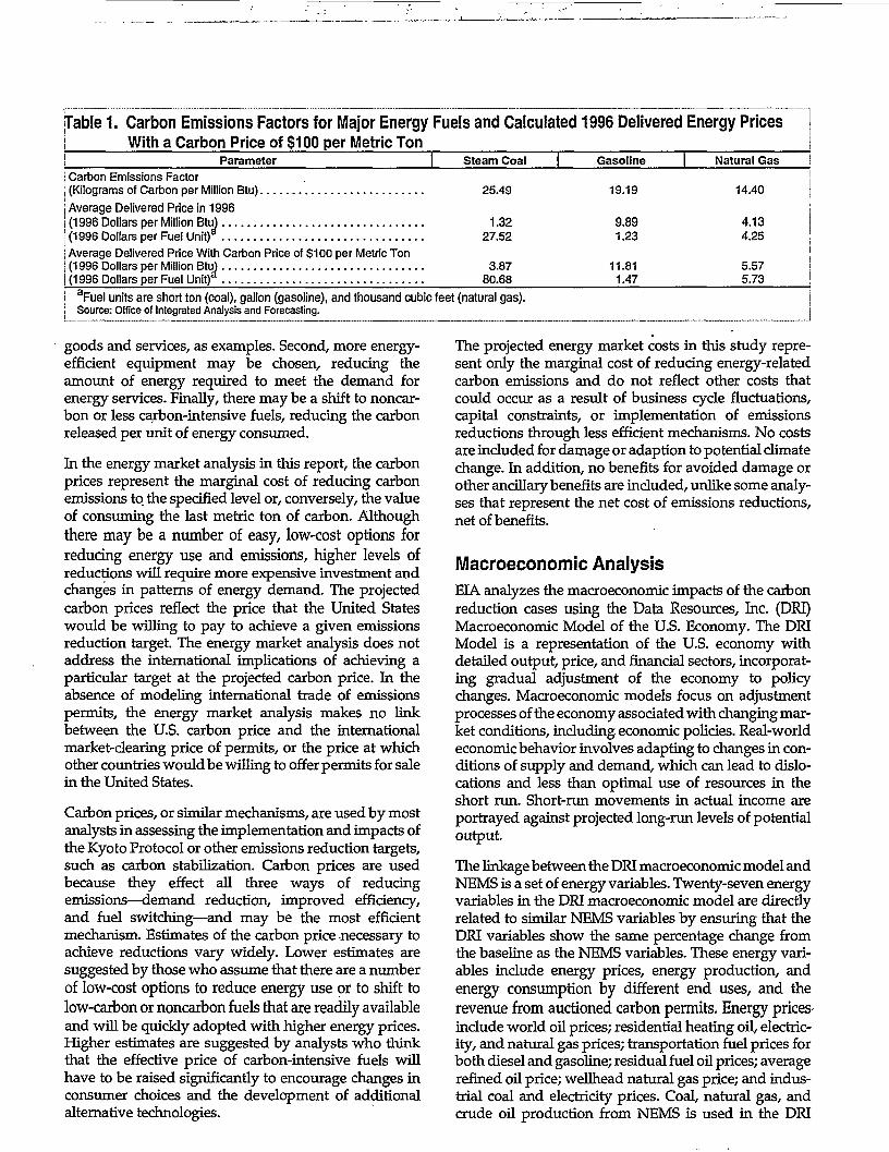
[Table 1. Carbon Emissions Factors for Major Energy Fuels and Calculated 1996 Delivered Energy PricesI With a Carbon Price of $100 per Metric TonI Parameter I Steam Coal | Gasoline | Natural Gas! Carbon Emissions Factor| (Kilograms of Carbon per Million Btu) 25.49 19.19 14.40
j Average Delivered Price in 19961(1996 Dollars per Million Btu) 1.32 9.89 4.13I (1996 Dollars per Fuel Unit)* 27.52 1.23 4.25| Average Delivered Price With Carbon Price of $100 per Metric TonI (1996 Dollars per Million Btu) 3.87 11.81 5.57I (1996 Dollars per Fuel Uni t / 80.68 JA7 5.73
j aFuel units are short ton (coal), gallon (gasoline), and thousand cubic feet (natural gas).j Source: Office of Integrated Analysis and Forecasting.
goods and services, as examples. Second, more energy-efficient equipment may be chosen, reducing theamount of energy required to meet the demand forenergy services. Finally, there may be a shift to noncar-bon or less carbon-intensive fuels, reducing the carbonreleased per unit of energy consumed.
In the energy market analysis in this report, the carbonprices represent the marginal cost of reducing carbonemissions to. the specified level or, conversely, the valueof consuming the last metric ton of carbon. Althoughthere may be a number of easy, low-cost options forreducing energy use and emissions, higher levels ofreductions will require more expensive investment andchanges in patterns of energy demand. The projectedcarbon prices reflect the price that the United Stateswould be willing to pay to achieve a given emissionsreduction target. The energy market analysis does notaddress the international implications of achieving aparticular target at the projected carbon price. In theabsence of modeling international trade of emissionspermits, the energy market analysis makes no linkbetween the U.S. carbon price and the internationalmarket-clearing price of permits, or the price at whichother countries would be willing to offer permits for salein the United States.
Carbon prices, or similar mechanisms, are used by mostanalysts in assessing the implementation and impacts ofthe Kyoto Protocol or other emissions reduction targets,such as carbon stabilization. Carbon prices are usedbecause they effect all three ways of reducingemissions—demand reduction, improved efficiency,and fuel switching—and may be the most efficientmechanism. Estimates of the carbon price necessary toachieve reductions vary widely. Lower estimates aresuggested by those who assume that there are a numberof low-cost options to reduce energy use or to shift tolow-carbon or noncarbon fuels that are readily availableand will be quickly adopted with higher energy prices.Higher estimates are suggested by analysts who thinkthat the effective price of carbon-intensive fuels willhave to be raised significantly to encourage changes inconsumer choices and the development of additionalalternative technologies.
The projected energy market costs in this study repre-sent only the marginal cost of reducing energy-relatedcarbon emissions and do not reflect other costs thatcould occur as a result of business cycle fluctuations,capital constraints, or implementation of emissionsreductions through less efficient mechanisms. No costsare included for damage or adaption to potential climatechange. In addition, no benefits for avoided damage orother ancillary benefits are included, unlike some analy-ses that represent the net cost of emissions reductions,net of benefits.
Macroeconomic AnalysisEIA analyzes the macroeconomic impacts of the carbonreduction cases using the Data Resources, Inc. (DRI)Macroeconomic Model of the U.S. Economy. The DRIModel is a representation of the U.S. economy withdetailed output, price, and financial sectors, incorporat-ing gradual adjustment of the economy to policychanges. Macroeconomic models focus on adjustmentprocesses of the economy associated with changing mar-ket conditions, including economic policies. Real-worldeconomic behavior involves adapting to changes in con-ditions of supply and demand, which can lead to dislo-cations and less than optimal use of resources in theshort run. Short-run movements in actual income areportrayed against projected long-run levels of potentialoutput.
The linkage between the DRI macroeconomic model andNEMS is a set of energy variables. Twenty-seven energyvariables in the DRI macroeconomic model are directlyrelated to similar NEMS variables by ensuring that theDRI variables show the same percentage change fromthe baseline as the NEMS variables. These energy vari-ables include energy prices, energy production, andenergy consumption by different end uses, and therevenue from auctioned carbon permits. Energy prices-include world oil prices; residential heating oil, electric-ity, and natural gas prices; transportation fuel prices forboth diesel and gasoline; residual fuel oil prices; averagerefined oil price; wellhead natural gas price; and indus-trial coal and electricity prices. Coal, natural gas, andcrude oil production from NEMS is used in the DRI

macroeconomic model as well as the end-use demandfor oil, natural gas, electricity, and coal.
Energy prices and end-use demands for fuels are the keyenergy inputs, along with the level of auctioned carbonrevenues, because energy prices affect inflation, and theend-use,fuel demand represents energy in the DRIaggregate production function, which describes the sup-ply potential of the economy. The amount of auctionedcarbon revenue dictates how much energy consumerscan expect to receive as rebated revenue, which in turnaffects disposable income. Changes in the values ofthese variables relative to the reference case would havemajor impacts on the macroeconomy.
When a system is developed for the trading of carbonpermits within the United States, a number of initialdecisions must be made: How many permits will beavailable? Will they be freely allocated or sold by com-petitive auction? If they are allocated, how will the initialallocations be made? If they are sold, what will be donewith the revenues? How many permits will be bought ininternational markets? If the permits are traded in a freemarket, holders of permits who can reduce carbon emis-sions at a cost below the permit price will sell their per-mits, and those with higher costs of reduction will buypermits, resulting in a transfer of funds between privateparties. If the permits are sold by competitive auction,there will be a transfer of funds from emitters of carbonto the Federal treasury. This analysis makes the explicitassumption that the permits will be sold in a competitiveauction run by the Federal Government.19
The macroeconomic analysis in Chapter 6 considers theflow of funds overseas that would be represented byinternational purchases of carbon permits, explicitlyassuming that the carbon price determined in the NEMSmodel is the international price at which permits wouldbe traded. Although the U.S. target established by theProtocol is a 7-percent reduction in greenhouse gasemissions relative to 1990 levels, the method of account-ing for sinks and the flexibility to use 1995 as the baseyear for the synthetic greenhouse gasses may mean thatthe reduction would be no more than 3 percent below1990 levels, according to the U.S. State Department. Thedifferences between the reduction level in the 1990-3%case and the reductions in the cases with higher levels ofenergy-related carbon emissions are assumed to be metby permits purchased in the international market at thecarbon price calculated for each case.
Many analyses of carbon mitigation have used a class ofmodels that are characterized as computable generalequilibrium (CGE) models. The CGE structure focuseson the interconnectedness of the economy and calculatesthe equilibrium of the economy in the long term,abstracting from the short-run adjustment processes.Most often the time horizon of these models is muchlonger—20,50, or 100 years into the future. In contrast,the DRI macroeconomic model used in this analysisfocuses on the adjustment of the economy over time,allowing for dislocations within the economy that yieldless than optimal levels of economic activity. While cli-mate change can arguably be considered a long-run phe-nomenon, the policies and measures to induce changemay take effect in a near-term horizon.
Chapter 7 gives a more detailed comparison of the simi-larities and differences in the alternative model struc-tures and results. Models of both types can contribute tothe assessment of the possible impacts on the economyof greenhouse gas reduction. However, past analyses ofthe issue using CGE and macroeconomic models haveoften disagreed with each other over the concepts of thefull employment GDP of the CGE models and the actualGDP measure presented in the macroeconomic models.Potential GDP is a concept calculated within the DRIModel but rarely presented as an output measure. Thediscussion in Chapter 6 considers the alternative viewsand introduces the concept of potential GDP into the dis-cussion of the economic impacts of the Protocol.
International Energy MarketsThe focus of the analysis is U.S. energy markets; how-ever, changes in international markets may have a sig-nificant influence on the United States. In particular,crude oil and petroleum products constitute an interna-tional market, and the world price of oil has a strongimpact on consumption and production of oil in theUnited States. Conversely, U.S. demand for and produc-tion of oil affects the world price of oil. The feedback ofU.S. oil markets on international markets is representedwithin the NEMS framework. World oil prices are deter-mined by means of a price reaction function, assumingthat the Organization of Petroleum Exporting Countrieswill expand oil production capacity to meet world oildemand.
For this analysis, it is assumed the other Annex I coun-tries will reduce their consumption of oil in order to helpmeet their reduction targets. Each country is assumed to
*'A permit auction system is identical to a carbon tax as long as the marginal abatement reduction cost is known with certainty by theFederal Government. If the target reduction is specified, as in this analysis, then there is one true price, which represents the marginal cost ofabatement, and this also becomes the appropriate tax rate. In the face of uncertainty, however, the actual tax rate applied may over- or un-dershoot the carbon reduction target. Auctioning of the permits by the Federal Government is evaluated in this report. To investigate a sys-tem of allocated permits would require an energy and macroeconomic modeling structure with a highly detailed sectoral breakout beyondthose represented in the NEMS and DRI models. For a comparison of emissions taxes and marketable permit systems, see R. Perman, Y. Ma,and J. McGilvray, Natural Resources and Environmental Economics (New York, NY: Longman Publishing, 1996), pp. 231-233.
Energy Information Administration / Impacts of the Kyoto Protocol on U.S. Energy Markets and Economic Activity 13
reduce its oil demand by the same percent that theUnited States reduces oil demand from the referencecase level. Oil consumption in non-Annex I countries isassumed to respond to changes in the world price of oilwith no additional reactions as a result of carbon reduc-tion policies.
Coal exports are a significant portion of U.S. coal pro-duction, with exports going to both Annex I and non-Annex I countries. Because Annex I countries mustreduce carbon emissions, it is assumed that coal produc-tion and imports in Western Europe and coal imports inJapan would be reduced and that coal consumption inthose countries would be reduced by more than theiremissions reductions in the Protocol. In the target caseswhere U.S. carbon emissions are allowed to rise above1990 levels in 2010, U.S. steam coal exports to Europe in2010 are assumed to be lower by 16 million tons, andexports to Asia are 4 million tons lower than in the refer-ence case. In the more stringent target cases, exports toEurope and Asia are 26 and 7 million tons lower, respec-tively, in 2010.
As a result of the Kyoto Protocol, energy prices in theAnnex I countries maybe higher than in the non-Annex Icountries, which do not have emissions reduction tar-gets in the Protocol. As a result, it is possible that moreenergy-intensive industries could shift from those coun-tries with higher energy costs. Energy-intensive indus-tries also may face reduced demand as consumers shifttheir consumption patterns to less energy-intensivegoods and services. Consequently, the composition ofU.S. industrial output is likely to change toward the lessenergy-intensive industries. Because this analysis doesnot cover international energy markets, internationaltrade, or the international activities of the Protocol, acomplete analysis of potential changes in U.S. industrialoutput is not possible (for discussion, see the box on"Industrial Composition" in Chapter 3).
Sensitivity Cases
A number of factors combine to determine the NEMSprojections of energy consumption and carbon emis-sions. Typically, AEO explores a wide range of cases thatvary the reference case assumptions on economicgrowth, world oil markets, technology improvement,and potential regulatory changes. In this analysis, a vari-ety of sensitivity cases are used to examine the factorsthat have the most significant impacts on energydemand and carbon emissions. With the exception of thenuclear power sensitivity case, all the sensitivity casesare analyzed relative to the 1990+9% case.
Low and High Economic GrowthThese cases analyze the effects of different assumptionsabout U.S. economic growth. The AEO98 reference case
assumes that the output of the Nation's economy, meas-ured by GDP, will increase by an average of 1.9 percent ayear between 1996 and 2020. The same assumption isused in all the carbon reduction cases in this analysis,although there is a feedback within the NEMS frame-work that alters the baseline economic assumptions as aresult of changes in energy prices. Therefore, as emis-sions reductions become more stringent and the result-ing carbon prices become higher, there will be areduction in economic growth.
In order to reflect the uncertainty in potential economicgrowth, AEO98 included high and low economicgrowth cases. The same alternative assumptions areused in this analysis. The high economic growth caseincludes higher population, labor force, and labor pro-ductivity,, resulting in higher industrial output, lowerinflation, and lower interest rates. As a result, the GDPincreases at an average rate of 2.4 percent a year through2020. The opposite assumptions in the low economicgrowth case lead to an average annual growth rate of 1.3percent.
Low and High TechnologyThese sensitivity cases examine the effects of assump-tions about the development and penetration of energy-consuming technologies on the analysis results. The ref-erence cases in this analysis and in AEO98 include con-tinued improvement in technologies for both energyconsumption and production—for example, improve-ments in building shell efficiencies for both new andexisting buildings; efficiency improvements for newappliances; productivity improvements for coal produc-tion; and improvements in the exploration and develop-ment costs, finding rates, and success rates for oil andgas production. Additional technology improvementsin the end-use demand sectors and in the electricity gen-eration sector could reduce energy consumption andenergy-related carbon emissions below their projectedlevels in the reference case. Conversely, slower improve-ment than that assumed in the reference could raise bothconsumption and emissions.
AEO98 presented alternative cases that varied keyassumptions concerning technology improvement andpenetration in the end-use demand and electricity gen-eration sectors. This analysis uses the same low technol-ogy assumptions for a low technology sensitivity. In theresidential and commercial sectors, it is assumed that allfuture equipment purchases will be made only from theequipment available in 1998 and that building shell effi-ciencies will be frozen at 1998 levels. Similarly, in thetransportation sector, efficiencies for new equipment arefixed at 1998 levels for all travel modes. In the industrialsector, plant and equipment efficiencies are fixed at 1998levels. No new advanced generation technologies areassumed to be available during the projection period.

Technology Improvement in the Reduction Cases and the Sensitivity Cases
In AEO98, energy intensity—primary energy con-sumption per dollar of GDP—is projected to declineby an annual average of 0.9 percent between 1996 and2020. This decline is significant but considerably lessthan the decline in the 1970s and early 1980s, whichaveraged 2.3 percent a year between 1970 and 1986.Approximately half the decline in energy intensityduring that period resulted from shifts in the econ-omy to service industries and other less energy-intensive industries; however, the other half of thedecline was due to the use of more energy-efficienttechnologies, resulting, in part, from the rapid escala-tion in the price of energy from the mid-1970sthrough the mid-1980s. The decline in energy inten-sity slowed during the late 1980s and early 1990s asthe growth in energy prices slowed and growth insome energy-intensive industries resumed. In the ref-erence case projections, continued modest increasesin the price of energy and growing demand for cer-tain energy services, such as appliances, office equip-ment, and travel, moderate further declines in energyintensity.
Energy intensity improvement results from opposingforces of growth in energy service demand andimprovement in the stock of energy-using equip-ment. New, more efficient technology must be devel-oped and available, but it also must be adopted inorder to contribute to energy efficiency improve-ments. Energy prices play a role in the consumer'sdecision when purchasing new equipment; however,other factors also influence equipment choice. Moreadvanced, energy-efficient technology is typicallymore expensive than standard equipment. The meth-odology for technology choice accounts for the rela-tive roles of first cost and energy cost savings over thelife of the equipment through the use of the discountrate, the implied payback period for the consumer
who is considering the choice of more efficientequipment. Perceived consumer preferences are alsoa factor in technology choice—for example, prefer-ences for larger, higher horsepower vehicles andlarger televisions, and for purchases of new heatingequipment that uses the same fuel as the equipment itreplaces. Improvements in energy intensity can beslowed by continued growth in energy serv-ices—more travel, household appliances, and officeequipment, larger homes, and higher industrial out-put—some of which are assumed to respond toenergy prices.
In the carbon reduction cases, energy prices rise withincreasingly stringent reduction targets. Intensityimprovements in those cases result both from reduc-tions in energy service demand and from the choice ofmore efficient equipment as a result of higher prices.These cases use the same assumptions of technologyavailability and characteristics. Additional researchand development in energy-efficient or alternativelyfueled technologies would likely expand the slate ofchoices available to consumers, leading to furtherimprovements in energy efficiency. The high technol-ogy case explores the impacts of improvements in theavailability, characteristics, and costs of technology asa result of increased research and development, thusseparating the impacts of energy prices and technol-ogy development.
Efficiency standards have contributed to pastimprovements in energy intensity. The CorporateAverage Fleet Efficiency and National ApplianceEnergy Conservation Act of 1987 standards, amongothers, are included in the AEO98 reference case;however, no new efficiency standards or improve-ments in current standards are assumed. The sameassumptions are used for all the carbon reduction andsensitivity cases in this analysis.
High technology assumptions were developed specifi-cally for this analysis by experts in technology engineer-ing for each of the energy-consuming sectors,considering the potential impacts of increased researchand development for more advanced technologies. Theassumptions include earlier years of introduction, lowercosts, high maximum market potential, and higher effi-ciencies than assumed in the reference case. In addition,the high technology sensitivity case includes carbonsequestration technology for coal- and natural-gas-firedgenerators to remove carbon dioxide and store it inunderground aquifers. By design, the effect of the hightechnology assumptions is distinct from the technologychanges that are induced by the higher energy prices inthe carbon reduction cases. Because the future costs of
the public and private investment that would be neededto develop and deploy more advanced technologies arenot known, they are not represented in the analysis;thus, the full economic cost may be understated. It ispossible that further technology improvements couldoccur beyond those represented in the high technologysensitivity case if a very aggressive research and devel-opment effort were established. Innovative, break-through technologies not foreseen in the analysis oftechnology could also be developed and lead toimprovements beyond those represented in the hightechnology assessment, but limited time is available forsuch technologies to become economically competitiveand achieve significant market share by 2010.
Energy Information Administration / Impacts of the Kyoto Protocol on U.S. Energy Markets and Economic Activity 15
New Nuclear Capacity
The nuclear power sensitivity case examines the role ofnuclear generation in reducing carbon emissions. InAEO98, electricity generation from nuclear plantsdeclines significantly over the forecast period. It isassumed that 65 units, about 51 percent of the totalnuclear capacity available in 1996, will be retired by2020. Twenty-four units are assumed to be retired beforethe end of their 40-year operating licenses, based onindustry announcements and analysis of the age andoperating costs of the units. No new nuclear plants are .constructed by 2020.
In all the carbon reduction cases, nuclear plants are life-extended if economical; however, in this sensitivity case,new nuclear plants can be built if they are economicallycompetitive with other generating technologies. In the1990+9% case, nuclear plants are not projected to be eco-nomically competitive with other plants. They dobecome competitive, however, with tike higher carbonprices projected in the 1990-3% case. Therefore, this sen-sitivity case is analyzed against the 1990-3% case.
Use of Models for Analysis
The reference case projections in both AEO98 and thisanalysis represent business-as-usual trend forecasts,given known trends in technology and demographics,current laws and regulations, and the specific method-ologies and assumptions used by EIA. Because EIA doesnot include future legislative and regulatory changes inits reference case projections, the projections provide apolicy-neutral baseline against which the impacts of pol-icy initiatives can be analyzed.
Results from any model or analysis are highly uncertain.By their nature, energy models are simplified represen-tations of complex energy markets. On the other hand,models provide a structured accounting framework thatallows analysts to capture the interrelationships of acomplex system in a consistent manner. Also, theassumptions and data underlying a model can be explic-itly cited, in contrast to a more ad hoc analysis. Theresults of any analysis depend on the specific data,assumptions, behavioral characteristics, methodologies,and model structures included. In addition, many of thefactors that will influence the future development ofenergy markets are inherently uncertain, includingweather, political and economic disruptions, technologydevelopment, and policy initiatives. Recognizing theseuncertainties, EIA has attempted in this study to isolate
and analyze the most important factors affecting futurecarbon emissions and carbon prices. The results of thevarious cases and sensitivities should be considered interms of the relative changes from the baseline caseswith which they are compared.
It has been suggested that models may be inherentlypessimistic in analyzing the potential impacts of policychanges. For example, in the Annual Energy Outlook 1993(AEO93),20 the first EIA analysis of CAAA90 compli-ance, the cost of a SO2 allowance was projected to be $423a ton in 2000, in 1996 dollars, rising to $751 a ton in 2010..Currently, the cost of an allowance is $95 a ton, andAEO98 projects that the cost will be $121 a ton in 2000and $189 in 2010. Projected coal prices in AEO98 are 34and 48 percent lower in 2000 and 2010, respectively, thanthose projected in AEO93, reflecting recent improve-ments in mine design and technology, economies ofscale in the mining industry, and lower transportationcosts induced by rail competition. There has been morefuel switching to low-sulfur, low-cost Western coal thanpreviously anticipated (it was initially assumed thatmany eastern coal-fired plants would not be able to burnwestern coal without considerable loss of performance).There has also been downward pressure on short-runallowance costs because generators have taken actionsto comply with the SO2 limitations earlier than antici-pated.2 Finally, technology improvements have low-ered the costs of flue-gas desulfurization technologies,or scrubbers, from $313 per kilowatt for scrubber retro-fitting as assumed in 1993 to $191 per kilowatt in 1998.The cost of SO2 compliance was overestimated to a largeextent because compliance relied on scrubbing, a rela-tively new technology with which there was little expe-rience. On the other hand, the current analysis of carbonreduction does not rely on a single technology but ratheron fuel switching and efficiency improvements, bothissues of long experience in energy markets.
In contrast, however, analyses of policies can also be toooptimistic. As noted earlier, reductions in greenhousegas emissions as a result of CCAP have been overesti-mated. In addition, some early analyses of the poten-tially beneficial impacts of price controls on oil andnatural gas proved in error because of the negativeeffects on production and competition in the industry.
A number of uncertainties may affect the costs of achiev-ing emissions reductions. As previously noted, the inter-pretation and implementation of many provisions of theKyoto Protocol are undetermined at this time. The flexi-bility allowed by the international activities may consid-erably lower the costs of the Protocol.
20Energy Information Administration, Annual Energy Outlook 1993, DOE/EIA-0383(93) (Washington, DC, January 1993).2 1 A.E. Smith, J. Platt, and A.D. Ellerman, "The Cost of Reducing SO2," Public Utilities Fortnightly (May 15,1998).

The availability and costs of technology remain one ofthe more significant factors in determining the cost ofemissions reductions, and this analysis seeks to quantifythat uncertainty to some degree with low and high tech-nology sensitivity cases. Although it is sometimeshypothesized that more cost-effective technologies aredeveloped once the requirements are established, itmust be noted that the cost and availability of some ofthe more advanced technologies in the reference case arenot certain, and even the reference assumptions may beoptimistic.
Although the Kyoto Protocol specifies reduction targets,signature and ratification by the United States wouldneed to be followed by the formulation of policies andprograms to achieve the carbon reductions. This analy-sis has chosen one possible mechanism, the impositionof a carbon fee with revenue recycling by two alternativemethods. Other programs—voluntary initiatives, man-datory standards, or other nonmarket policies—couldresult in higher or lower costs. Even with a carbon fee,other fiscal policies for recycling the revenues, includingnot recycling, are likely to have different impacts on theU.S. economy.
The timing of policy initiatives may also be an importantfactor in the cost of emissions reductions. Given that theKyoto Protocol includes a specific timetable for reducingemissions, policies and initiatives that begin earlier mayallow for more gradual adoption and a less costly transi-tion, particularly if consumers react with foresight ofanticipated price increases and emissions restrictions.Consumer response to anticipated or realized priceincreases and other policy initiatives is likely to beanother significant determinant of the cost of the KyotoProtocol. Finally, other energy policies formulated forpurposes other than the Protocol, such as electricityindustry restructuring and other emissions controls,may have ancillary impacts on carbon emissions.
In the next chapter, Chapter 2, the results from thecarbon emissions reduction cases and the sensitivitycases are summarized. Chapters 3 through 6 presentmore detailed analysis of the results for the end-usedemand sectors, electricity generation, fossil fuelmarkets, and the macroeconomy, respectively. Chapter7 concludes with a comparison of this analysis andsimilar studies of the costs of carbon emissionsreductions.
Energy Information Administration / Impacts of the Kyoto Protocol on U.S. Energy Markets and Economic Activity 17

This page is intentionally left blank.

2. Summary of Energy Market Results
This chapter summarizes the energy market results ofthe carbon reduction and sensitivity cases evaluating theeffects of the Kyoto Protocol in the National EnergyModeling System (NEMS). The first set of cases examinethe impacts of six carbon emissions reduction targets,relative to a reference case without the Kyoto Protocol,as described in Chapter 1. The remaining cases examinethe sensitivity of those results to variations in keyassumptions—the macroeconomic growth rate, the rateof technological progress, and the role of nuclear power.More detailed analyses of the energy market results arepresented in Chapters 3, 4, and 5. The macroeconomicresults are described in Chapter 6. Although the resultsof the carbon reduction cases are consistent with theassumptions made, the projected impacts are subject toconsiderable uncertainty—particularly with the more
stringent carbon reduction targets—because the casesreflect significant changes in energy markets.
Carbon Reduction Cases
Carbon PricesUnder the Kyoto Protocol, the United States is commit-ted to reducing greenhouse gas emissions to 7 percentbelow 1990 levels in the period 2008 through 2012. Thereduction in energy-related carbon emissions that theUnited States must achieve to comply with the green-house gas reduction target in the Protocol depends onthe level of emissions offsets credited for sinks, reduc-tions in other greenhouse gases, international permittrading, joint implementation, and the Clean Develop-ment Mechanism (CDM). A set of six cases examines arange of carbon emissions reduction targets, rangingfrom 7 percent below 1990 levels, an average of 1,250million metric tons during the period 2008 to 2012, to 24percent above 1990 levels, or an average of 1,670 millionmetric tons. The most stringent case assumes that thetarget of reducing greenhouse gases to 7 percent below1990 levels is the domestic goal for energy-related car-bon emissions, with no offsets from sinks, offsets, inter-national trade, the CDM, or compensating changes inother greenhouse gases.
The six carbon reduction cases are compared against areference case similar to the one published in the AnnualEnergy Outlook 1998 (AEO98) (Figure 1). The Protocolindicates that the greenhouse gas reductions must be
achieved on average in each of the years between 2008and 2012, and the targets are assumed to hold onaverage for that period. At the specification of theCommittee, the targets were held constant after 2012through the forecast horizon of 2020. To provide energymarkets time to adjust, mandatory carbon reductiontargets were phased in beginning in 2005, the year whenthe Protocol indicates that progress toward compliancemust be demonstrated.
Figure 1. Projections of Carbon Emissions,1990-2020
Million Metric TonsReference
1990+24%1990+14%1990+9%19901990-76A
12,000 -
11,500-
11,000-
500-
1990 1995 2000 2005 2010 2015 2020
Sources: History: Energy Information Administration, Emissions o(Greenhouse Gases in the United States 1996, DOE/ElA-0573(96) (Washington,PC, October 1997). Projections: Office of Integrated Analysis and Forecasting,National Energy Modeling System runs KYBASE.P080398A, FD24ABV,P080398B, FO1998.P080398B, FD09ABV.D080398B, FD1990.O080398B,FD03BLW.D080398B, and FP07BLW.D080398B.
In order to reduce carbon emissions, demand for energyservices must be reduced, more efficient energy-consuming technologies used, or less carbon-intensivefuels consumed. Thus, to constrain the overall level ofcarbon emissions to a given target, a price on carbonemissions is included in the delivered price of fuels. Thecarbon price is equivalent to the cost of a carbon permitunder a market-based program within the United Statesto regulate the overall level of carbon emissions. In sucha program, the purchase of fossil fuels would require theexchange of carbon permits, and a market for carbonpermits would operate to allocate the overall supply ofpermits among U.S. energy consumers. More restrictivecarbon targets would lead to higher market-clearingprices for carbon.
Energy Information Administration / Impacts of the Kyoto Protocol on U.S. Energy Markets and Economic Activity 19

In analyzing the carbon emissions reduction targets, thecarbon prices are incorporated as an added cost of con-suming energy; that is, as an increase in the deliveredprice of energy. The added cost is in direct proportion tothe carbon permit price and the carbon content of thefuel consumed. As a result, energy consumers facehigher energy costs—both for the fossil fuels they con-sume directly, such as gasoline, and for the indirect useof fossil energy used to generate electricity. The higherenergy costs also affect the cost of producing goods andservices throughout the economy and, as a result, havemacroeconomic effects beyond the impacts on theenergy sector.
As indicated in Figure 1, some carbon reductions occurbefore 2005, based on anticipatory behavior, primarilyas a result of forward-looking capacity planning deci-sions assumed in the electricity industry. For the elec-tricity industry, where fossil fuel purchases are apredominant operating cost, planners are assumed toincorporate future fuel costs in their economic evalua-tion of generating plant alternatives.22 As a result, somecapacity choices reflected in the reference case before2005 are altered in the carbon reduction cases based oncarbon prices beginning in 2005, thus lowering carbonemissions before the assumed start of carbon permittrading.
Table 2 presents a summary of the key results in 2010and 2020 for the reference case, the 24-percent-above-1990 (1990+24%) case, the 9-percent-above-1990(1990+9%) case, and the 3-percent-below-1990 (1990-3%)case. Tables of the complete results for all the carbonreduction cases are included in Appendix B.
Figure 2 depicts the estimated carbon prices, in constant1996 dollars, necessary to achieve the carbon emissionsreduction targets. Generally, the highest permit priceoccurs early on in the commitment period. The carbonprice declines over time as cumulative investments inmore energy-efficient and lower-carbon equipment,particularly in the electricity generation industry, tendto reduce the marginal cost of compliance in later years.
For most of the cases, the trend of carbon prices includessome relatively minor year-to-year fluctuations. Also,particularly in the more stringent reduction cases, thecarbon price generally peaks in 2008, the first year of thecommitment .period, because of the 3-year phase-inperiod. A longer adjustment period might reduce theprice; however, early reductions do not count towardthe required reductions in the commitment period. Insome cases, 1- to 2-year declines in prices occur as
Figure 2. Projections of Carbon Prices, 1996-2020j 1996 Dollars per Metric Ton
1995 2000 2005 2010 2015 2020
I Source: Office of Integrated Analysis and Forecasting, National EnergyModeling System runs KYBASE.D080398A, FD24ABV.D080398B, FD1998/D080398B, FD09ABV.D080398B, FD1990.D080398B. FD03BLW.D080398B,'and FD07BLW.D080398B.
electricity generators complete construction of low-carbon replacement plants. The new plants allowgenerators to shift from coal to lower-carbon energysources, reducing their need to purchase carbon permitsand holding down carbon prices. Because the additionsof replacement capacity occur in discrete amounts, theyear-to-year changes in carbon prices can be somewhatuneven. The short-term fluctuations in projected carbonprices are consistent with, but probably understate, thedegree of short-term price movements that would beexpected in a market for carbon permits.
The carbon prices from 2008 to 2012 average $159 permetric ton in the 1990+9% case, which represents acarbon reduction averaging 325 million metric tons ayear relative to the reference case (Figure 3). In the morestringent 1990-3% case, the average carbon price from2008 to 2012 is $290 per metric ton, achieving an averageannual carbon reduction during that period of 485million metric tons. In the 1990+24% case, carbon pricesaverage $65 per metric ton in the compliance period,with average carbon reductions of 122 million metrictons.
Carbon prices decline in most of the cases after2012, despite continued growth in the demand forenergy as the carbon target is held constant. Whileincreased energy demand would be expected toexert upward pressure on carbon prices over time,downward pressure results from the cumulative effectof investments to improve energy efficiency andswitch to lower-carbon energy sources. These long-lived
^The modeling approach assumes perfect foresight of carbon prices for capacity planning in the electricity industry. Perfect foresight, inthis context, means that the carbon prices that are anticipated during planning are later realized. An algorithm solves for the path of carbonprices in which anticipated and realized carbon prices are approximately the same, while ensuring that the carbon prices clear the carbonpermit market each year. In the end-use demand sectors, foresight is assumed not to have a material influence on energy equipment deci-sions, and such decisions are modeled on the basis of prices in effect at the time of the decision.
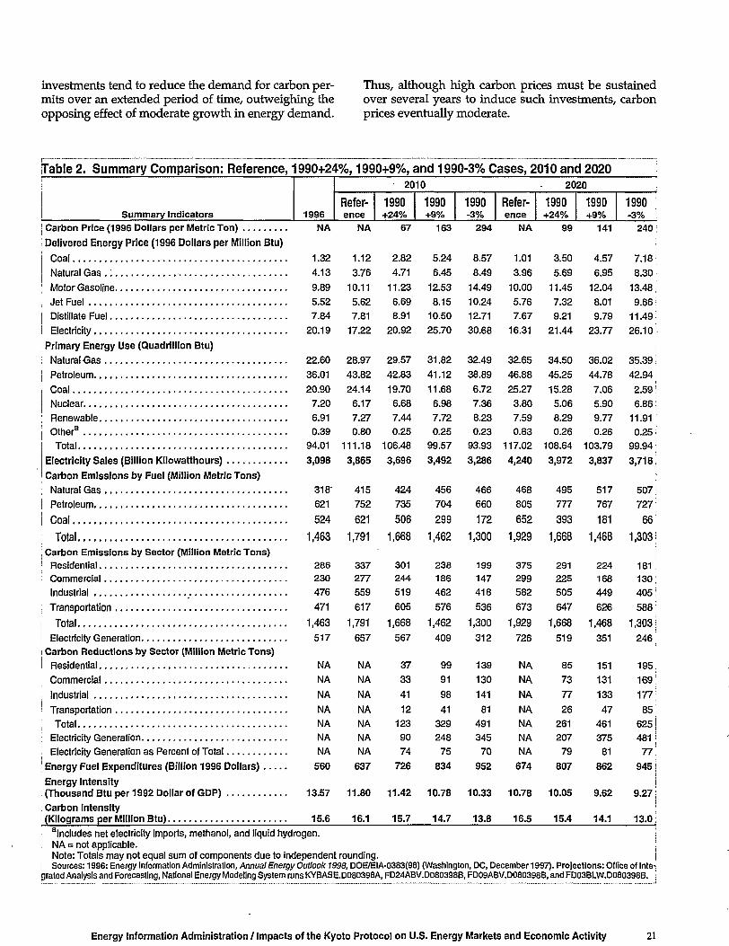
investments tend to reduce the demand for carbon per-mits over an extended period of time, outweighing theopposing effect of moderate growth in energy demand.
Thus, although high carbon prices must be sustainedover several years to induce such investments, carbonprices eventually moderate.
[Table 2. Summary Comparison: Reference, 1990+24%, 1990+9%, and 1990-3% Cases, 2010 and 2020
Summary IndicatorsCarbon Price (1996 Dollars per Metric Ton)
Delivered Energy Price (1996 Dollars per Million Btu)
Coal
Natural Gas . ,
Motor Gasoline
Jet Fuel
Distillate Fuel
Electricity
Primary Energy Use (Quadrillion Btu)
1996NA
1.32
4.13
9.89
5.52
7.84
20.19
Refer-ence
NA
1.12
3.76
10.11
5.62
7.81
17.22
2010
1990+24%
67
2.82
4.71
11.23
6.69
8.91
20.92
1990+9%
163
5.24
6.45
12.53
8.1510.50
25.70
1990-3%
294
8.57
8.49
14.49
10.2412.71
30.68
Refer-ence
NA
1.01
3.96
10.00
5.767.67
16.31
2020
1990+24%
99
3.50
5.69
11.45
7.32
9 21
21.44
1990+9%
141
4.57
6.95
12.04
8.019 79
23.77
1990-3%
240
7.18
8 30
13.48
9 66
11 49
26.10
Natural Gas
Petroleum
Coal
Nuclear
; Renewable
I Othera
| Total
Electricity Sales (Billion Kilowatthours)
Carbon Emissions by Fuel (Million Metric Tons)
Natural Gas
Petroleum
Coal
TotalCarbon Emissions by Sector (Million Metric Tons)
ResidentialCommercialIndustrial
Transportation
Total
Electricity Generation
Carbon Reductions by Sector (Million Metric Tons)Residential
Commercial
Industrial
Transportation
Total
Electricity Generation
Electricity Generation as Percent of Total
Energy Fuel Expenditures (Billion 1996 Dollars).. .
Energy Intensity(Thousand Btu per 1992 Dollar of GDP)
Carbon Intensity(Kilograms per Million Btu)
22.60
36.01
20.907.206.910.39
28.97 29.57
43.82 42.83
24.14 19.70
6.17 6.68
7.27 7.44
0.80 0.2594.01 111.18 106.48
3,098 3,865 3,696
31.82
41.12
11.68
6.987.720.25
99.57
32.4938.89
6.727.368.230.23
93.933,492 3,286
32.65 34.5046.88 45.25
25.27 15.283.80 5.06
7.59 8.29
0.83 0.26117.02 108.64
4,240 3,972
36.0244.787.065.909.770.26
103.79
286230476471
337277559617
301
244
519
605
238
186
462
576
1,463 1,791 1,668 1,462
517 657 567 409
NA
NA
NA
NA
NA
NA
NA
560
NA
NA
NA
NA
NA
NA
NA
637
37
33
41
12
123
90
74
726
9991
98
41
329248
75
834
199
147
418
536
1,300
312
139
130
141
81
491
345
70
952
375299582673
291
225
505
647
224168449626
13.57 11.80 11.42 10.78 10.33 10.78 10.05 9.62
15.6 16.1 15.7 14.7 13.8 16.5 15.4 14.1
35.39 j
42.94 •2.59|6.86 i
11.91 I0.25!
99.94;3,837 3,718;
318' 415 424 456 466 468 495 517 5071
621 752 735 704 660 805 777 767 727:
524 621 506 299 172 652 393 181 66;1,463 1,791 1,668 1,462 1,300 1,929 1,668 1,468 1,303 i
181:130:
405!
588 !
1,929 1,668 1,468 1,303!
726 519 351
NA 85 151
NA 73 131
NA 77 133
NA 26 47
NA 261 461
NA 207 375
NA 79 81
674 807 862
246
195!
169!
177;
85;
625!
481 j
77!
945 |j
9.27;
13.0!
includes net electricity imports, methanol, and liquid hydrogen. !NA = not applicable. :Note: Totals may not equal sum of components due to independent rounding. jSources: 1996: Energy Information Administration, Annual Energy Outlook 1998, DOE/EIA-0383(98) (Washington, DC, December 1997). Projections: Office of Inte^
grated Analysis and Forecasting, National Energy Modeling System runs KYBASE.D080398A, FD24ABV.D080398B, FD09ABV.D080398B, and FD03BLW.D080398B. i
Energy Information Administration / Impacts of the Kyoto Protocol on U.S. Energy Markets and Economic Activity 21

Figure 3. Average Annual Carbon EmissionReductions and Projected Carbon Prices,2008-2012
3 5 0 -
300 -
250-
200-
150-
100-
5 0 -
Average Carbon Price (1996 Dollars per Metric Ton)H 990-7%
^1990-3%
F1990
H 990+9%
"1990+14%
"1990+24%
''Reference
I 0 100 200 300 400 500 600
i Average Carbon Reductions (Million Metric Tons)i! Source: Office of Integrated Analysis and Forecasting, National EnergyModeling System runs KYBASE.D080398A, FD24ABV.D080398B, FD1998"D080398B, FD09ABV.D080398B, FD1990.D080398B, FD03BLW.D080398B'and FD07BLW.D080398B. I
Energy Prices
With the carbon prices included in the delivered cost ofenergy, the prices under the various carbon targets risesignificantly above the reference case. Figures 4,5, and 6show the average delivered prices of coal, natural gas,petroleum, and electricity in the 1990+24%, the 1990+9%and the 1990-3% cases, respectively. In percentageterms, coal prices are most affected by the carbon prices,with the delivered price of coal in the 1990+9% caseincreasing 346 to 368 percent above the reference caseprice in the 2008 to 2012 period (Figure 7). Natural gasprices in the 1990+9% case increase 64 to 74 percentabove the reference case prices, and oil prices increaseby 25 to 29 percent. Electricity prices, reflecting thehigher costs of fossil fuels used for generation, as well asthe incremental cost of additional plant investments toreduce carbon emissions by replacing coal-fired plants,increase to 47 to 50 percent above the reference caselevel.
Compared with the changes in coal and natural gasprices, the average increase in electricity prices is rela-tively low. Larger amounts of electricity would be gen-erated from renewable and nuclear power, for whichfuel costs are unaffected by carbon prices. In addition,cost-of-service electricity pricing is assumed for most ofthe country, so that fuel costs would be only a partialdeterminant of electricity prices. Nonfuel operating and
maintenance costs and capital equipment costs have alarger role in setting electricity prices under cost-of-service pricing. In regions where electricity prices areassumed to be set competitively on the basis of marginalcosts (California, New York, and New England), carbonprices would have a more significant influence on elec-tricity prices, particularly when coal-fired plants are themarginal generators. On the other hand, those regionsare less dependent on coal than are many other areas ofthe country. -
The pattern of projected delivered energy pricesmatches the trend for carbon prices, especially in themore restrictive carbon reduction cases. In these cases,the carbon prices become a dominant component of thedelivered cost of fossil energy; however, market forcescontinue to play a role in energy prices, especially forpetroleum products. The reduced demand for oil underthe various carbon reduction targets tends to reduceworld oil prices. World oil prices are projected to fall asdemand is reduced in the United States and in otherdeveloped countries that are committed to reducingemissions under the Kyoto Protocol. In 2010, world oilprices are projected to be about $20.00 per barrel in the1990+24% case, $18.70 in the 1990+9% case, and $17.80 inthe 1990-3% case, as compared with $20.80 per barrel inthe reference case. With lower world oil prices, thechange in delivered petroleum product prices with thevarious carbon prices is not as high as for natural gasprices, despite the higher carbon content of petroleum.
In contrast to petroleum, coal prices are unlikely to bemoderated by competitive forces. Much of the demandfor coal by electricity generators is eliminated in the car-bon reduction cases, particularly with the more strin-gent targets. Coal consumption for other uses, includingindustrial steam coal and metallurgical coal, is alsoreduced but on a smaller percentage basis than for elec-tricity generation. Although coal produced for export isalso lower in the carbon reduction cases due to lowerdemand in the Annex I nations, the change is relativelysmall in comparison with the reductions in productionfor domestic use. Coal exports, projected at 113 millionshort tons in 2010 in the reference case, are 89 millionshort tons in 2010 in the 1990+24% and 1990+9% casesand 76 million short tons in the 1990-3% case. Becausethe industrial and export coal markets are served pri-marily by eastern coal producers, eastern productiondeclines less in the carbon reduction cases than does pro-duction from western mines, which primarily serve theelectricity generation market. Thus, while regionalminemouth prices generally decline in the carbon re-duction cases relative to the reference case, the national
23 A related factor influencing the effect of carbon prices on gasoline demand is that the price of gasoline already includes Federal andState excise taxes averaging 37 cents per gallon in 1996, equivalent to a carbon permit price of $155 per metric ton. When additional carbonpermit prices are included in the delivered price of gasoline, the percentage increase in price is not as high as it would be if gasoline were un-taxed initially. In turn, the percentage change in gasoline demand due to the carbon price is not as high as it would be if gasoline were not al-ready taxed.
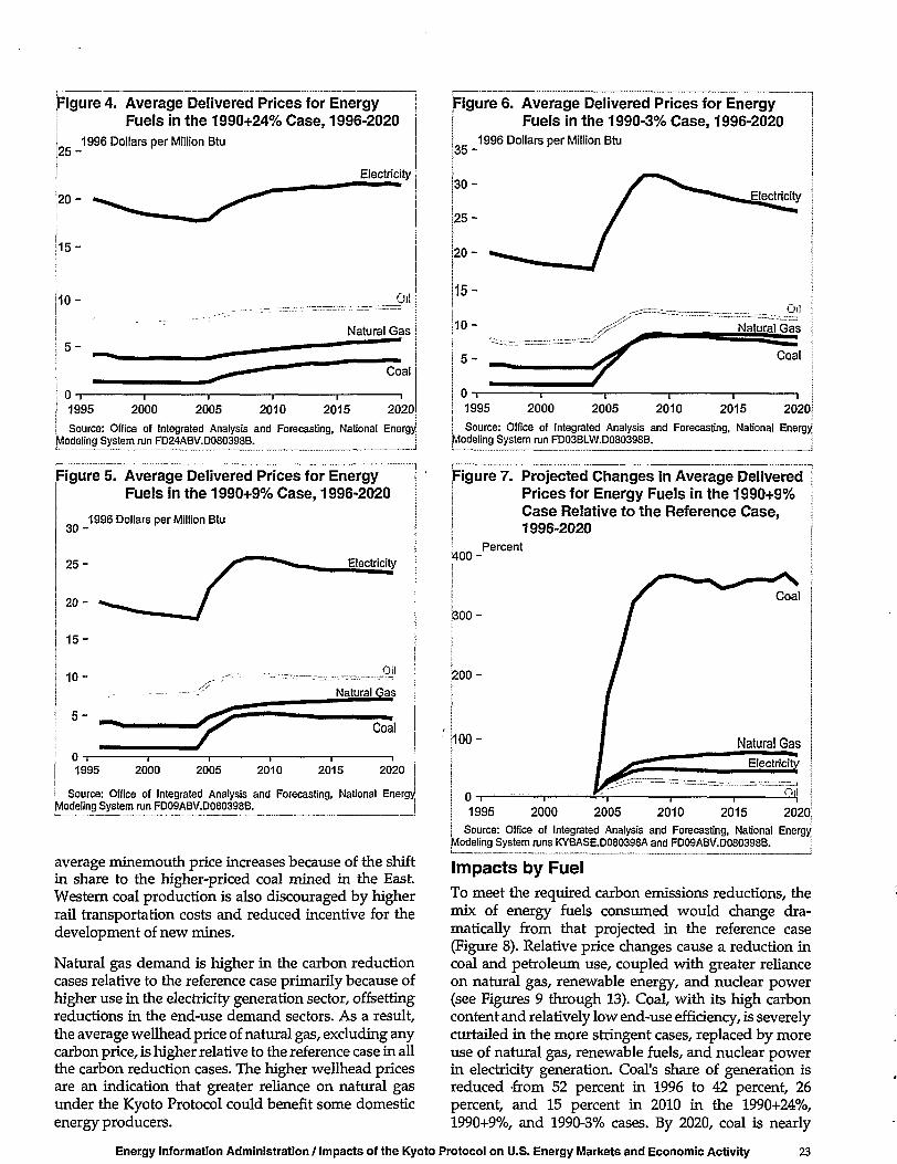
Figure 4. Average Delivered Prices for EnergyFuels in the 1990+24% Case, 1996-2020
1996 Dollars per Million Btu
2010 2015 2020
Source: Office of Integrated Analysis and Forecasting, National EnergyModeling System run FD24ABV.D080398B.
:igure 5. Average Delivered Prices for EnergyFuels in the 1990+9% Case, 1996-2020
3 0 -
2 5 -
1996 Dollars per Million Btu
Electricity
10-
Coal
1995 2000 2005 2010 2015 2020
| Source: Office of Integrated Analysis and Forecasting, National Energy1
Modeling System run FD09ABV.D080398B. |
average minemouth price increases because of the shiftin share to the higher-priced coal mined in the East.Western coal production is also discouraged by higherrail transportation costs and reduced incentive for thedevelopment of new mines.
Natural gas demand is higher in the carbon reductioncases relative to the reference case primarily because ofhigher use in the electricity generation sector, offsettingreductions in the end-use demand sectors. As a result,the average wellhead price of natural gas, excluding anycarbon price, is higher relative to the reference case in allthe carbon reduction cases. The higher wellhead pricesare an indication that greater reliance on natural gasunder the Kyoto Protocol could benefit some domesticenergy producers.
Figure 6. Average Delivered Prices for Energy! Fuels in the 1990-3% Case, 1996-2020
Source: Office of Integrated Analysis and Forecasting, National EnergyModeling System run FD03BLW.D080398B.
1996 Dollars per Million Btu
Electricity j
1995 2000 2005 2010 2015 2020
Figure 7. Projected Changes in Average DeliveredPrices for Energy Fuels in the 1990+9%Case Relative to the Reference Case,1996-2020
'400-
3 0 0 -
• 2 0 0 -
Hoo-
Percent
Coal •
1995 2000 2005 2010 2015 2020!
Source: Office of Integrated Analysis and Forecasting, National EnergyModeling System runs KYBASE.D080398A and FD09ABV.D080398B. I
Impacts by FuelTo meet the required carbon emissions reductions, themix of energy fuels consumed would change dra-matically from that projected in the reference case(Figure 8). Relative price changes cause a reduction incoal and petroleum use, coupled with greater relianceon natural gas, renewable energy, and nuclear power(see Figures 9 through 13). Coal, with its high carboncontent and relatively low end-use efficiency, is severelycurtailed in the more stringent cases, replaced by moreuse of natural gas, renewable fuels, and nuclear powerin electricity generation. Coal's share of generation isreduced -from 52 percent in 1996 to 42 percent, 26percent, and 15 percent in 2010 in the 1990+24%,1990+9%, and 1990-3% cases. By 2020, coal is nearly
Energy Information Administration / Impacts of the Kyoto Protocol on U.S. Energy Markets and Economic Activity 23
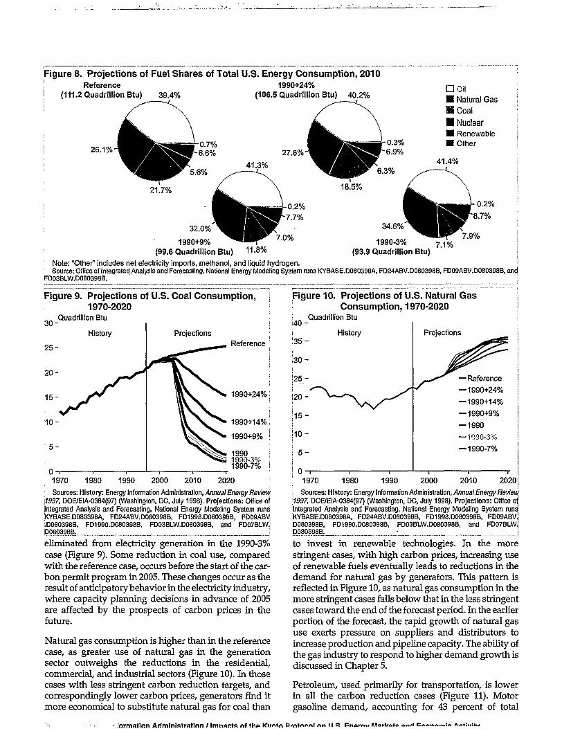
Figure 8. Projections of Fuel Shares of Total U.S. Energy Consumption, 2010Reference
(111.2 Quadrillion Btu) 39.4%
1990+24%
(106.5 Quadrillion Btu) 40.2%
26.1%
• Oil• Natural GasHCoal• Nuclear• Renewable• Other
41.4%
1990+9%
(99.6 Quadrillion Btu) 11-8%1990-3%
(93.9 Quadrillion Btu)
7.9%7.1%
Note: "Other" includes net electricity imports, methanol, and liquid hydrogen.Source: Office of Integrated Analysis and Forecasting, National Energy Modeling System runs KYBASE.D080398A, FD24ABV.D080398B, FD09ABV.D080398B, ancl
FD03BLW.D080398B.
30
25
20
15
10
5
0
Quadrillion Btu
History
-
-
Projections
"IN.
Figure 9. Projections of U.S. Coal Consumption,1970-2020
Reference
1990+24%
1990+14%
1990+9%
19901990-3%1990-7%
1970 1980 1990 2000 2010 2020
Sources: History: Energy Information Administration, Annual Energy Review\1997, DOE/EIA-0384(97) (Washington, DC, July 1998). Projections: Office ofIntegrated Analysis and Forecasting, National Energy Modeling System runsKYBASE.D080398A, FD24ABV.D080398B, FD1998.D080398B, FD09ABV;.D080398B, FD1990.D080398B, FD03BLW.D080398B, and FD07BLW.D080398B. j
eliminated from electricity generation in the 1990-3%case (Figure 9). Some reduction in coal use, comparedwith the reference case, occurs before the start of the car-bon permit program in 2005. These changes occur as theresult of anticipatory behavior in the electricity industry,where capacity planning decisions in advance of 2005are affected by the prospects of carbon prices in thefuture.
Natural gas consumption is higher than in the referencecase, as greater use of natural gas in the generationsector outweighs the reductions in the residential,commercial, and industrial sectors (Figure 10). In thosecases with less stringent carbon reduction targets, andcorrespondingly lower carbon prices, generators find itmore economical to substitute natural gas for coal than
Figure 10. Projections of U.S. Natural GasConsumption, 1970-2020
4 0 -
3 5 -
Quadrillion Btu
History Projections
—Reference
— 1990+24%
— 1990+14%
— 1990+9%
— 1990
— 1990-3%
— 1990-7%
1970 1980 1990 2000 2010 2020
Sources: History: Energy Information Administration, Annual Energy Revlev/1997, DOE/EIA-0384(97) (Washington, DC, July 1998). Projections: Office ofIntegrated Analysis and Forecasting, National Energy Modeling System runskYBASE.D080398A, FD24ABV.D080398B, FD1998.D080398B, FD09ABV,'D080398B, FD1990.D080398B, FD03BLW.D080398B, and FD07BLW^DJD80398R : i
to invest in renewable technologies. In the morestringent cases, with high carbon prices, increasing useof renewable fuels eventually leads to reductions in thedemand for natural gas by generators. This pattern isreflected in Figure 10, as natural gas consumption in themore stringent cases falls below that in the less stringentcases toward the end of the forecast period. In the earlierportion of the forecast, the rapid growth of natural gasuse exerts pressure on suppliers and distributors toincrease production and pipeline capacity. The ability ofthe gas industry to respond to higher demand growth isdiscussed in Chapter 5.
Petroleum, used primarily for transportation, is lowerin all the carbon reduction cases (Figure 11). Motorgasoline demand, accounting for 43 percent of total
ormation Administration / Imnants of the> Kvntn Prntnnnl nn 11 « Cnormi »mi c»«nnm:~ *«•:..:*..

figure 11. Projections of U.S. Petroleum| Consumption, 1970-2020
5 0 -
4 5 -
(40 -
J35 -3 0 -
1J25-
120-
J 1 O -5 -
Quadrillion Btu
History
0
Projections
—Reference
— 1990+24%
— 1990+14%
—1990+9%
—1990
—1990-3%
— 1990-7%
1970 1980 1990 2000 2010 2020
j Sources: History: Energy Information Administration, Annual Energy ReviewI7997, DOE/EIA-0384(97) (Washington, DC, July 1998). Projections: Office ofIntegrated Analysis and Forecasting, National Energy Modeling System runs)<YBASE.D080398A1 FD24ABV.D080398B, FD1998.D080398B, FD09ABV.P080398B, FD1990.D080398B, FD03BLW.D080398B. and FD07BLW.D080398B.
petroleum consumption in 1996, is lower by 15 percentin 2010 in the 1990-3% case, by 8 percent in the 1990+9%case, and by 3 percent in the 1990+24% case than in thereference case. Consumers respond to higher gasolineprices by reducing miles driven and purchasing moreefficient vehicles.
Nuclear power, which produces no carbon emissions,becomes more attractive under carbon reduction targets.While no new nuclear plants are allowed to be built inthe carbon reduction cases, extending the lifetimes ofexisting plants is projected to become more economicalwith higher carbon prices. In the reference case,approximately half of the nuclear capacity now inoperation is expected to be retired by 2020, reducing U.S.nuclear capacity by 53 gigawatts between 1996 and 2020.Much of that capacity would be life-extended in thecarbon reduction cases (15 gigawatts, 26 gigawatts, and38 gigawatts in the 1990+24%, 1990+9%, and 1990-3%cases, respectively). As a result, the use of nuclear powerfor electricity generation is projected to be higher in allthree cases than in the reference case (Figure 12).
Consumption of renewable.energy, which results in nonet carbon emissions, is projected to be higher withcarbon reduction targets (Figure 13). Most of theincrease is in electricity generation, primarily withadditions to wind energy systems and an increase in theuse of biomass (wood, switchgrass, and refuse). Theshare of generation supplied by renewables increasesfrom 9 percent in 2020 in the reference case to 11 percent,15 percent, and 20 percent in the 1990+24%, 1990+9%,and 1990-3% cases, respectively. Most of the increase inrenewable generation occurs after the 2008-2012compliance period, reflecting a relatively prolonged
Figure 12. Projections of U.S. Nuclear EnergyConsumption, 1970-2020
Quadrillion Btu
1990-7%1990-3%19901990+9%1990+14%
1990+24%
Reference
1970 1980 1990 2000 2010 2020Sources: History: Energy Information Administration, Annual Energy Review
1997, DOE/EIA-0384(97) (Washington, DC, July 1998). Projections: Office ofIntegrated Analysis and Forecasting, National Energy Modeling System runsKYBASE.D080398A, FD24ABV.D080398B, FD1998.D080398B, FD09ABVJD080398B, FD1990.D080398B, FD03BLW.D080398B, and FD07BLWJD080398B. !
Figure 13. Projections of U.S. Renewable EnergyConsumption, 1990-2020
Quadrillion Btu
1990-7%1990-3% |1990 ''1990+9% '1990+14% ;1990+24% :Reference i
1990 1995 2000 2005 2010 2015 2020 iSources: History: Energy Information Administration, Annual Energy Review
[1997, DOE/EIA-0384(97) (Washington, DC, July 1998). Projections: Office ofIntegrated Analysis and Forecasting, National Energy Modeling System runsJKYBASE.D080398A, FD24ABV.D080398B, FD1998.D080398B, FD09ABV.D080398B, FD1990.D080398B, FD03BLW.D080398B, and FD07BLW.D080398B.! j
period of market penetration as renewable technologycosts and performance improve over time.
Electricity generation, which accounted for 35 percent ofenergy-related carbon emissions in 1996, is also sig-nificantly lower across all the cases (Figure 14). In the1990-3% case, electricity sales in 2010 are 15 percentbelow the reference case projection, with percentagereductions of about 13 percent occurring in the resi-dential and industrial sectors and about 19 percent in thecommercial sector. The relative changes in electricity
Energy Information Administration / Impacts of the Kyoto Protocol on U.S. Energy Markets and Economic Activity 25
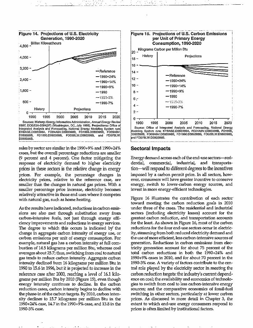
Figure 14. Projections of U.S. Electricityi Generation, 1990-2020
Billion Kilowatthours4.800 -
J4.000 -
3,200 -
2,400 -
1,600-
8 0 0 -
0-History
—Reference
—1990+24%
— 1990+14%
—1990+9%
— 1990
— 1930-3%
—1990-7%
Projections
1990 1995 2000 2005 2010 2015 2020JSources: History: Energy Information Administration, Annual Energy Review
\I997, DOE/EIA-0384(97) (Washington, DC, July 1998). Projections: Office ofIntegrated Analysis and Forecasting, National Energy Modeling System runsKYBASE.D080398A, FD24ABV.D080398B, FD1998.D080398B, FD09ABVJD080398B, FD1990.D080398B, FD03BLW.D080398B, and FD07BLWJD080398B.
sales by sector are similar in the 1990+9% and 1990+24%cases, but the overall percentage reductions are smaller(9 percent and 4 percent). One factor mitigating theresponse of electricity demand to higher electricityprices in these sectors is the relative change in energyprices. For example, the percentage changes inelectricity prices, relative to the reference case, aresmaller than the changes in natural gas prices. With asmaller percentage price increase, electricity becomesrelatively attractive in those end uses where it competeswith natural gas, such as home heating.
As the results have indicated, reductions in carbon emis-sions are also met through substitution away fromcarbon-intensive fuels, not just through energy effi-ciency improvements and reductions in energy services.The degree to which this occurs is indicated by thechange in aggregate carbon intensity of energy use, orcarbon emissions per unit of energy consumption. Forexample, natural gas has a carbon intensity at full com-bustion of 14.5 kilograms per million Btu, whereas coalaverages about 25.7; thus, switching from coal to naturalgas tends to reduce carbon intensity. Aggregate carbonintensity declined from 16 kilograms per million Btu in1990 to 15.6 in 1996, but it is projected to increase in thereference case after 2000, reaching a level of 16.1 kilo-grams per million Btu by 2010 (Figure 15), even thoughenergy intensity continues to decline. In the carbonreduction cases, carbon intensity begins to decline withthe phase-in of the carbon targets. By 2010, carbon inten-sity declines to 15.7 kilograms per million Btu in the1990+24% case, 14.7 in the 1990+9% case, and 13.8 in the1990-3% case.
Figure 15. Projections of U.S. Carbon Emissionsper Unit of Primary EnergyConsumption, 1990-2020
2 0 -Kilograms Carbon per Million Btu
History
14-
12-
10-
8 -
6.-
4 -
2 -
Projections
—Reference
—1990+24%
—1990+14%
— 1990+9%
— 1990
—1350-3%
— 1990-7%
1990 1995 2000 2005 2010 2015 2020
Source: Office of Integrated Analysis and Forecasting, National EnergyModeling System runs KYBASE.D080398A, FD24ABV.D080398B, FD1998.D080398B, FD09ABV.D080398B, FD1990.D080398B, FD03BLW.D080398B,and FD07BLW.D080398B.i I
Sectoral Impacts
Energy demand across each of the end-use sectors—resi-dential, commercial, industrial, and transporta-tion—will respond to different degrees to the incentivesimposed by a carbon permit price. In all sectors, how-ever, consumers will have greater incentive to conserveenergy, switch to lower-carbon energy sources, andinvest in more energy-efficient technologies.
Figure 16 illustrates the contribution of each sector'toward meeting the carbon reduction goals in 2010under three of the cases. The residential and industrialsectors (including electricity losses) account for thegreatest carbon reduction, and transportation accountsfor the least. As shown in Figure 16, most of the carbonreductions for the four end-use sectors occur in electric-ity, stemming from both reduced electricity demand andthe use of more efficient, less carbon-intensive sources ofgeneration. Reductions in carbon emissions from elec-tricity generation account for about 75 percent of thetotal carbon reductions in both the 1990+24% and1990+9% cases in 2010, and for about 70 percent in the1990-3% case. A variety of factors contribute to the cen-tral role played by the electricity sector in meeting the
carbon reduction targets: the industry's current depend-ence on coal; the availability and economics of technolo-gies to switch from coal to less carbon-intensive energysources; and the comparative economics of fossil-fuelswitching in other sectors, particularly at lower carbonprices. As discussed in more detail in Chapter 3, theextent to which end-use energy consumers respond toprices is often limited by institutional factors.

figure 16. Projected Reductions in CarbonEmissions by End-Use Sector Relativeto the Reference Case, 2010
1160-
1120-
1990+9%
Million Metric Tons1990+24%
•i'ion-£lectnc• Electric
80-
40-
sg
ra1CD
I
tria
l
•o—
ition
I
rans
p
ntia
l
CD
Res
CD
'2
Com
tria
l
snp
—
ition
o
rans
p
Dtia
l;id
ei
»CD
cr
co•p
mei
Com
trial
snp 1ra
nsp
Note: Electricity emissions are from the fuels used to generate elec-itricity and are attributed to the sectors relative to their shares of totalElectricity consumption.I Source: Office of Integrated Analysis and Forecasting, National EnergyModeling System runs KYBASE.D080398A, FD24ABV.D080398B, FD09ABVJp080398B, and FD03BLW.D080398B.
In the industrial sector, some of the carbon reductionscan be attributed to reductions in manufacturing outputthat result from the impact of higher energy prices on theeconomy. In addition, industrial firms respond byreplacing productive capacity faster, investing in moreefficient technology, and switching to less carbon-intensive fuels. Improvements in efficiency areindicated by reductions in energy intensity, as measuredby the energy use per dollar of gross domestic product(GDP). In 2010, industrial energy intensity is reducedfrom 4.2 million Btu per dollar of GDP in the referencecase to 4.1 million Btu per dollar in the 1990+24% case,4.0 million Btu per dollar in the 1990+9% case, and 3.9million Btu per dollar in the 1990-3% case (Figure 17).Taking into account fuel switching and efficiencyimprovements, carbon emissions per unit of GDP in2010 for the industrial sector are reduced from 60kilograms per thousand dollars of GDP in the referencecase to 55,50, and 46 kilograms per thousand dollars ofGDP in the 1990+24%, 1990+9%, and 1990-3% cases,respectively.
Carbon reductions in the transportation sector occurprimarily as the result of reduced travel and thepurchase of more efficient vehicles in response to higherenergy prices. Compared with the reference case, light-duty vehicle travel (cars, vans, pickup trucks, and sport-utility vehicles) in 2010 is lower by 1 percent in the1990+24% case, by 5 percent in the 1990+9% case, and by11 percent in the 1990-3% case (Figure 18). At the sametime, more efficient cars and light trucks are purchased,raising overall fleet efficiency (Figure 19). In 2010, theaverage fuel efficiency for the light-duty vehicle fleet is20.7, 21.2, and 21.5 miles per gallon in the 1990+24%,
Figure 17. Projections of U.S. Industrial Energy| Intensity, 1996-2020
5.0-Thousand Btu per 1992 Dollar of GDP
3 . 5 -
J 3 . 0 -
J 2 . 5 -
k(1.5-
1.0-
0 . 5 -
—Reference
—1990+24%
—1990+14%
—1990+9%
—1990
— 1390-3%
—1990-7%
1995 2000 2005 2010 2015 2020Source: Office of Integrated Analysis and Forecasting, National Energy,
Modeling System runs KYBASE.D080398A, FD24ABV.D080398B, FD1998.D080398B, FD09ABV.D080398B, FD1990.D080398B, FD03BLW.D080398B,and FD07BLW.D080398B.
Figure 18. Projections of U.S. Light-Duty Vehicle! Travel, 1996-2020
3,500 -j
j 3,000 -
12.500 -
2,000 -
11,500-
1,000-
5 0 0 -
Billion Vehicle-Miles Traveled
—Reference— 1990+24%
— 1990+14%
— 1990+9%
- 1 9 9 0
—1990-7%
1995 2000 2005 2010 2015 2020| Source: Office of Integrated Analysis and Forecasting, National EnergyModeling System runs KYBASE.D080398A, FD24ABV.D080398B, FD1998,1
P080398B, FD09ABV.D080398B, FD1990.D080398B, FD03BLW.D080398BIand FD07BLW.D080398B..
1990+9%, and 1990-3% cases, respectively, comparedwith 20.5 miles per gallon in the reference case. Theresults of those increases are reductions of 3 percent, 8percent, and 15 percent, respectively, from the referencecase level of motor gasoline demand in 2010 (Figure 20).Travel reductions and efficiency improvements alsooccur in the air and freight sectors, further reducingcarbon emissions. Overall, transportation energyconsumption in 2010 is lower by 2 percent in the1990+24% case, by 6 percent in the 1990+9% case, and by12 percent in the 1990-3% case, than in the reference case.
In the residential and commercial sectors, higher energyprices encourage investments in more efficient equip-ment and building shells and also reduce the demand
Energy Information Administration / Impacts of the Kyoto Protocol on U.S. Energy Markets and Economic Activity 27
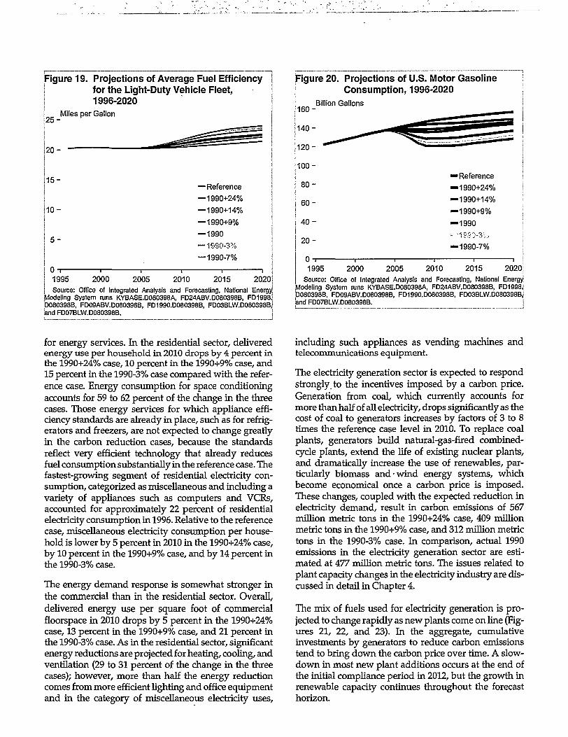
Figure 19. Projections of Average Fuel Efficiency |for the Light-Duty Vehicle Fleet, I1996-2020 I
2 5 -
2 0 -
[15 -
ho-
5 -
Miles per Gallon
- Reference
-1990+24%
-1990+14%
-1990+9%
•1990
-1990-3%
-1990-7%
1995 2000 2005 2010 2015 2020!
Source: Office of Integrated Analysis and Forecasting, National EnergyModeling System runs KYBASE.D080398A, FD24ABV.D080398B, FD1998JD080398B, FD09ABV.D080398B, FD1990.D080398B, FD03BLW.D080398BJand FD07BLW.D080398B. I
Figure 20. Projections of U.S. Motor GasolineConsumption, 1996-2020
160-
140-
120-
100-
8 0 -
6 0 -
4 0 -
2 0 -
Billion Gallons
•Reference
•1990+24%
•1990+14%
•1990+9%
•1990
-1SS0-3c,;
-1990-7%
1995 2000 2005 2010 2015 2020
Source: Office of Integrated Analysis and Forecasting, National EnergyModeling System runs KYBASE.D080398A, FD24ABV.D080398B, FD1998,D080398B, FD09ABV.D080398B, FD1990.D080398B, FD03BLW.D080398B,'and FD07BLW.D080398B.
J
for energy services. In the residential sector, deliveredenergy use per household in 2010 drops by 4 percent inthe 1990+24% case, 10 percent in the 1990+9% case, and15 percent in the 1990-3% case compared with the refer-ence case. Energy consumption for space conditioningaccounts for 59 to 62 percent of the change in the threecases. Those energy services for which appliance effi-ciency standards are already in place, such as for refrig-erators and freezers, are not expected to change greatlyin the carbon reduction cases, because the standardsreflect very efficient technology that already reducesfuel consumption substantially in the reference case. Thefastest-growing segment of residential electricity con-sumption, categorized as miscellaneous and including avariety of appliances such as computers and VCRs,accounted for approximately 22 percent of residentialelectricity consumption in 1996. Relative to the referencecase, miscellaneous electricity consumption per house-hold is lower by 5 percent in 2010 in the 1990+24% case,by 10 percent in the 1990+9% case, and by 14 percent inthe 1990-3% case.
The energy demand response is somewhat stronger inthe commercial than in the residential sector. Overall,delivered energy use per square foot of commercialfloorspace in 2010 drops by 5 percent in the 1990+24%case, 13 percent in the 1990+9% case, and 21 percent inthe 1990-3% case. As in the residential sector, significantenergy reductions are projected for heating, cooling, andventilation (29 to 31 percent of the change in the threecases); however, more than half the energy reductioncomes from more efficient lighting and office equipmentand in the category of miscellaneous electricity uses,
including such appliances as vending machines andtelecommunications equipment.
The electricity generation sector is expected to respondstrongly, to the incentives imposed by a carbon price.Generation from coal, which currently accounts formore than half of all electricity, drops significantly as thecost of coal to generators increases by factors of 3 to 8times the reference case level in 2010. To replace coalplants, generators build natural-gas-fired combined-cycle plants, extend the life of existing nuclear plants,and dramatically increase the use of renewables, par-ticularly biomass and wind energy systems, whichbecome economical once a carbon price is imposed.These changes, coupled with the expected reduction inelectricity demand, result in carbon emissions of 567million metric tons in the 1990+24% case, 409 millionmetric tons in the 1990+9% case, and 312 million metrictons in the 1990-3% case. In comparison, actual 1990emissions in the electricity generation sector are esti-mated at 477 million metric tons. The issues related toplant capacity changes in the electricity industry are dis-cussed in detail in Chapter 4.
The mix of fuels used for electridty generation is pro-jected to change rapidly as new plants come on line (Fig-ures 21, 22, and 23). In the aggregate, cumulativeinvestments by generators to reduce carbon emissionstend to bring down the carbon price over time. A slow-down in most new plant additions occurs at the end ofthe initial compliance period in 2012, but the growth inrenewable capacity continues throughout the forecasthorizon.

Figure 21. Projected Fuel Use for ElectricityGeneration by Fuel in the 1990+24%Case, 1996-2020
Quadrillion Btu
Source: Office of Integrated Analysis and Forecasting, National EnergyModeling System run FD24ABV.D080398B.
Renewable/OtherHydropoweri
Nuclear
Natural Gas
Coal
2000 2005 2010 2015 2020
Figure 23. Projected Fuel Use for ElectricityGeneration by Fuel in the 1990-3% Case,1996-2020
Renewable/Other
Hydropower
Nuclearr: !
Natural Gas
Source: Office of Integrated Analysis and Forecasting, National EnergyModeling System run FD03BLW.D080398B.
Figure 22. Projected Fuel Use for ElectricityGeneration by Fuel in the 1990+9%Case, 1996-2020
Quadrillion Btu
Renewable/Other
Hydropower;
Nuclear
Natural Gas
Coal
2000 2005 2010 2015 2020Source: Office of Integrated Analysis and Forecasting, National Energy
Modeling System run FD09ABV.D080398B.
Sensitivity CasesAmong the sources of uncertainty in the effects of car-bon mitigation polices over the next 20 years are theassumed rate of economic growth, the speed of adoptionof advanced technologies, and the role of nuclear power.A series of sensitivity cases illustrate how these factorsinfluence the results of the carbon reduction cases. Thesensitivity cases were analyzed against the 1990+9%case. The nuclear power sensitivity case was analyzedagainst the 1990-3% case, because new nuclear powerplants were found to be economical only with the highercarbon prices in that case.
Because each of the sensitivity cases is constrained to thesame level of carbon emissions as the case to which it iscompared, the primary impact is not on the carbon emis-sions levels, or even aggregate energy consumption, butrather on the carbon prices required to meet the emis-sions target. For example, in the high technology case,with an emissions reduction target of 9 percent above1990 levels, projected carbon emissions during the com-pliance period are the same as in the corresponding ref-erence technology case (1990+9%) with emissions at thesame level. What differs is the cost of meeting the target,as reflected in the required carbon price or in expendi-tures for energy services. As a result, the carbon priceand energy expenditures are the primary measures bywhich the sensitivity cases are compared in this report,in contrast to the presentation of similar sensitivities inAEO98. Because the technology sensitivities in the AEOtypically are run with energy prices and macroeconomicassumptions held constant and without any target forcarbon emissions, sensitivities are normally comparedon the basis of levels of energy consumption.
Macroeconomic GrowthThe assumed rate of economic growth has a strongimpact on the projection of energy consumption and,therefore, on the projected levels of carbon emissions. InAEO98, the high economic growth case includes highergrowth in population, the labor force, and labor produc-tivity, resulting in higher industrial output, lower infla-tion, and lower interest rates. As a result, GDP increasesat an average rate of 2.4 percent a year from 1996 to 2020,compared with a growth rate of 1.9 percent a year in thereference case. With higher macroeconomic growth,energy demand grows more rapidly, as higher manufac-turing output and higher income increase the demandfor energy services. In AEO98, total energy consumption
Energy Information Administration / Impacts of the Kyoto Protocol on U.S. Energy Markets and Economic Activity 29

in the high economic growth case is 117 quadrillion Btuin 2010, compared with 112 quadrillion Btu in the refer-ence case. Carbon emissions are 80 million metric tons,or 4 percent; higher than the reference case level of 1,803million metric tons.
Assumptions of lower growth in population, the laborforce, and labor productivity result in an average annualgrowth rate of 1.3 percent in the AEO98 low economicgrowth case between 1996 and 2020. With lower eco-nomic growth, energy consumption in 2010 is reducedfrom 112 quadrillion Btu to 107 quadrillion Btu, and car-bon emissions are 90 million metric tons, or 5 percent,lower than in the reference case. Thus, the effect ofhigher or lower macroeconomic growth can have a sig-nificant impact on the ease or difficulty of meeting thecarbon targets.
To reflect the uncertainty of potential economic growth,high and low economic growth sensitivity cases wereanalyzed against the 1990+9% case, using the samehigher and lower economic growth assumptions as inAEO98. With higher economic growth, the industrialoutput and energy service demand are higher. As aresult, carbon prices must be correspondingly higher toattain a given carbon emissions target. With low eco-nomic growth, the effects are reversed, leading to lowercarbon prices. In addition to industrial output, some ofthe most important economic drivers in NEMS are dis-posable personal income, housing stock, housing size,commercial floorspace, industrial output, light-dutyvehicle sales, and travel.
Figure 24 shows the effect of the high and lowmacroeconomic growth assumptions on the projectionsfor 2010 in the 1990+9% case. The carbon price in 2010 is$215 per metric ton in the high economic growth case, or$52 per metric ton higher than the price of $163 permetric ton in the 1990+9% case with reference economicgrowth. In the low economic growth case, the carbonpermit price in 2010 is $128 per metric ton or $35 permetric ton lower than in the 1990+9% case.
The higher carbon prices necessary to achieve the carbonreductions with higher economic growth will tend tomoderate the growth rates of the economy as a wholeand the economic drivers in the energy system. Despitethis price effect, total energy consumption in 2010 ishigher with higher economic growth, by 2.2 quadrillionBtu relative to the 1990+9% with reference economicgrowth. Similarly, the lower economic growth assump-tion results in lower carbon prices, which offset a portionof the projected reduction in energy consumption thatwould otherwise be expected when economic growthslows. Lower economic growth lowers total energy con-sumption by 2.2 quadrillion Btu.
To meet a carbon reduction target with higher economicgrowth and energy consumption, there is a shift to less
Figure 24. Projected Carbon Prices in the 1990+9%High and Low Economic Growth andHigh and Low Technology Sensitivity |Cases, 2010 :
1996 Dollars per Metric Ton
2 5 0 -
215
243
Low Reference High Low Reference High
Growth Growth Growth Tech- Tech- Tech-nology nology nology
Source: Office of Integrated Analysis and Forecasting, National EnergyModeling System runs FD09ABV.D080398B, LMAC09.D080698A, HMAC09jP080598A, FREEZE09.D080798A, and HITECH09.D080698A. j
carbon-intensive fuels and higher energy efficiency;however, economic growth affects energy consumptionin the industrial and transportation sectors more signifi-cantly than in the other end-use sectors. With higher eco-nomic growth, renewable energy and natural gasconsumption is higher, primarily for generation but alsoin the industrial sector. Coal use for generation is lower,and more nuclear capacity is life-extended as a result ofthe higher carbon prices. Petroleum consumption is alsohigher with higher economic growth, in both the trans-portation and industrial sectors. As shares of totalenergy consumption, natural gas and renewables arehigher with higher economic growth, coal is lower, andnuclear and petroleum remain approximately the same.Opposite trends for fuel consumption and fuel sharesare seen when lower economic growth is assumed.
Total energy intensity is lower in the high economicgrowth case, partially offsetting the changes in energyconsumption caused by the different growth assump-tions. There are three reasons for the improvement inenergy intensity. First, although demand for energyservices is higher with higher economic growth, there isgreater opportunity to turn over and improve the stockof energy-using technologies. In the AEO98 cases, aggre-gate energy efficiency in the high economic growth casedecreases at a rate of 1.0 percent a year through 2020,compared with 0.9 percent in the reference case and 0.8percent in the low economic growth case. Second, withhigher carbon prices, additional efficiency improve-ments are induced by higher energy prices. Finally, thehigher energy prices lead to some reductions in energyservice demand, moderating the impacts of higher eco-nomic growth. In the 1990+9% carbon reduction case,aggregate energy intensity declines at an average annualrate of 1.6 percent through 2010. In the 1990+9% high
economic growth sensitivity case, the annual declineincreases to 1.9 percent. In the 1990+9% low economicgrowth case, the decline in energy intensity slows to 1.3percent per year.
Technological ProgressThe assumed rate of development and penetration ofenergy-using technology has a significant impact onprojected energy consumption and energy-related car-bon emissions. Faster development of more energy-efficient or lower carbon-emitting technologies thanassumed in the reference case could reduce both con-sumption and emissions; however, because the AEO98reference case already assumes continued improvementin both energy consumption and production technolo-gies, slower technological development is also possible.
To examine the influence of technology improvement,two sensitivity cases were analyzed relative to the1990+9% case. The high technology case includes moreoptimistic assumptions on the costs, efficiencies, marketpotential, and year of availability for the more advancedgenerating and end-use technologies, assumingincreased research and development activity. This sensi-tivity case also assumes a carbon sequestration technol-ogy for coal- and natural-gas-fired electricity generation,which would capture the carbon dioxide emitted duringfuel combustion and store it in underground aquifers;however, use of the technology is not projected to be eco-nomical relative to other technologies within the timeframe of this sensitivity case because of high operatingcosts and storage difficulties. The low technology caseassumes that all future equipment choices are madefrom the end-use and generation equipment available in1998, with building shell and industrial plant efficienciesfrozen at 1998 levels.
Because faster technology development makesadvanced energy-efficient and low-carbon technologiesmore economically attractive, the carbon prices requiredto meet carbon reduction levels are reduced. Con-versely, slower technology improvement requireshigher carbon prices (Figure 24). In the 1990+9% casewith high technology assumptions, the carbon price in2010 is $121 per metric ton—$42 per metric ton lowerthan the price of $163 per metric ton in the 1990+9% casewith reference technology assumptions. With the lowtechnology assumptions, the projected carbon price is$243 per metric ton in 2010.
Total energy consumption in 2010 is lower by 2.1 quad-rillion Btu in the high technology case, about 2 percentbelow the projection in the 1990+9% case, and averageenergy prices, including carbon prices, are 10 percentlower. As a result, direct expenditures on energy are 13percent lower in the high technology case. Demand inboth the industrial and transportation sectors is lower asefficiency improvements in industrial processes and
most transportation modes outweigh the countervailingeffects of lower energy prices. In the residential andcommercial sectors, the effect of lower energy prices bal-ances the effect of advanced technology, and consump-tion levels are at or near those in the 1990+9% case. Withthe high technology assumptions in the generation sec-tor, coupled with the lower carbon permit price, coal usefor generation is 3.8 quadrillion Btu higher than the 9.7quadrillion Btu level associated with reference technol-ogy assumptions.
In the low technology case, the converse trends prevail.In 2010, total consumption is higher by 1.5 quadrillionBtu with the low technology assumptions, and energyexpenditures are 17 percent higher. Industrial and trans-portation demand is higher, and residential and com-mercial demand lower, suggesting that industry andtransportation are more sensitive to technology changesthan to price changes, and that the residential and com-mercial sectors are more sensitive to price changes. Withthe higher carbon prices in the low technology case, coaluse is further reduced in the generation sector, withmore natural gas, nuclear power, and renewables usedto meet the carbon reduction targets.
Nuclear PowerIn the AEO98 reference case, nuclear generation declinessignificantly, because 52 percent of the total nuclearcapacity available in 1996 is expected to be retired by2020. A number of units are retired before the end oftheir 40-year operating licenses, based on industryannouncements and analysis of the age and operatingcosts of the units. In the carbon reduction cases, lifeextension of the plants can occur, if economical, andthere is an increasing incentive to invest in nuclear plantrefurbishment with higher carbon prices; however, noconstruction of new nuclear power plants is assumed,given continuing high capital investment costs and insti-tutional constraints associated with nuclear power.
A nuclear power sensitivity case was developed toexamine the potential contribution of new nuclear plantconstruction to carbon emissions reductions, assumingthat new nuclear capacity would be built when it waseconomically competitive with other generating tech-nologies. In the nuclear power sensitivity case, electric-ity generators were assumed to add nuclear powerplants when it became economical to do so. In addition,the reference case assumptions about higher costsincurred for the first few advanced nuclear plants wererelaxed by reducing the premium in costs for the firstphase of new nuclear plant additions.
In the 1990+9% case, even with the nuclear power sensi-tivity assumptions, nuclear plants are not competitivewith fossil and renewable plants. In the 1990-3% case,however, when the new nuclear assumptions are used,1 gigawatt of new nuclear capacity is added by 2010, and
Energy Information Administration / Impacts of the Kyoto Protocol on U.S. Energy Markets and Economic Activity 31

41 gigawatts, representing about 68 new plants of 600megawatts each, are added by 2020. (In a. trial case inwhich first-generation cost premiums were left un-changed, only 3 gigawatts of nuclear capacity wasadded.) The availability of this no-carbon capacity off-sets about 25 million metric tons of carbon emissionsfrom additional natural gas plants in 2020; on the otherhand, more coal is used, because the projected carbonprices are lower. Most of the impact from the newnuclear plants comes after the commitment period of2008 through 2012. As a result, there is little impact oncarbon prices in 2010. By 2020, however, carbon prices
are $199 per metric ton with the assumption of newnuclear plants, as compared with $240 per metricton in the 1990-3% case with the reference nuclearassumptions.
In the 1990-3% case, total energy consumption is aboutthe same in 2010 with new nuclear plants allowed andhigher by about 1.8 quadrillion Btu in 2020. Somewhatlower energy prices induce higher consumption in allsectors, and the greater availability of carbon-freenuclear generation allows the carbon reduction target tobe met with higher end-use consumption.

3. End-Use Energy Demand
BackgroundThis chapter provides in-depth analyses of the carbonemissions reduction cases for the four end-use demandsectors—residential, commercial, industrial, and trans-portation. Additional analyses are included for anumber of alternative cases, including low and hightechnology sensitivity cases, which have the most directimpacts on energy end use.
Primary and Delivered EnergyConsumption
In each of the reduction cases, carbon emissions arereduced through a combination of switching to carbon-free or lower-carbon fuels, reductions in energy services,and increased energy efficiency. The latter two optionslower total energy consumption (Figure 25).
Electricity generation typically consumes about threetimes as much energy, on the basis of British thermalunits (Btu), as is contained in the electricity delivered tofinal consumers. In AEO98, total delivered energyconsumption in 1996 is estimated at 70.4 quadrillion Btu,compared with total primary energy consumption of94.0 quadrillion Btu (Table 3). The difference comes fromelectricity-related generation and transmission lossesand, consequently, is relatively small for the trans-portation sector, where little electricity is consumed.Although the delivered price of electricity per Btugenerally is more than three times the delivered price ofother energy sources, the convenience and efficiency ofelectricity use outweigh the price difference for manyapplications.
Because consumers base their fuel and equipmentchoices on performance at the point of use, the analysisof end-use energy consumption presented in thischapter focuses on energy delivered to final consumers.When consumers choose to purchase a particular type of
Figure 25. Projections of Primary EnergyConsumption, 1990-2020
Quadrillion BtuH20-
100-
80 -
60 -
4 0 -
2 0 -
—Reference
—1990+24%
—1990+14%
—1990+9%
—1990
—1990-3%
—1990-7%
0 - . . 1 > 1 • .
1990 1995 2000 2005 2010 2015 2020
Sources: History: Energy Information Administration, Annual Energy -Review\I997, DOE/EIA-0384(97) (Washington, DC. July 1998). Projections: Office ofIntegrated Analysis and Forecasting, National Energy Modeling System rungKYBASE.D080398A, FD24ABV.D080398B, FD1998.D080398B, FD09ABVJD080398B, FD1990.D080398B, FD03BLW.D080398B, FP07BLW.D080398B. ;
energy-consuming equipment or to use a particular fuel,their decisions are based on the cost and performancecharacteristics of the technology, mandated efficiencystandards, and energy prices. End-use energy pricesinclude all the direct costs of providing energy to thepoint of use.
The distinction between end-use and primary energyconsumption is an important one for the evaluation ofefficiency standards and other energy policies. Reduc-ing electricity demand through the use of more efficienttechnologies reduces primary energy consumption by afactor of three. In addition, although electricity at itspoint of use produces no carbon emissions, reductions inelectricity use produce savings in emissions from thefuels used for its generation.
Table 3. Primary and End-Use Energy Consumption
Sector
Residential
Commercial
Industrial
Transportation
Total
by Sector, 1996End-Use Consumption
Quadrillion Btu
11.1
7.5
27.1
24.7
70.4
| Percent of Total
16
11
38
35
100
Primary Consumption
Quadrillion Btu |
19.4
15.0
34.8
24.9
94.0Source: Energy Information Administration, Annual Energy Outlook 1998, DOE/EIA-0383(98) (Washington, DC, December 1997).
Percent of Total
21
16
37
26
100
t*t-*-*i -.« n
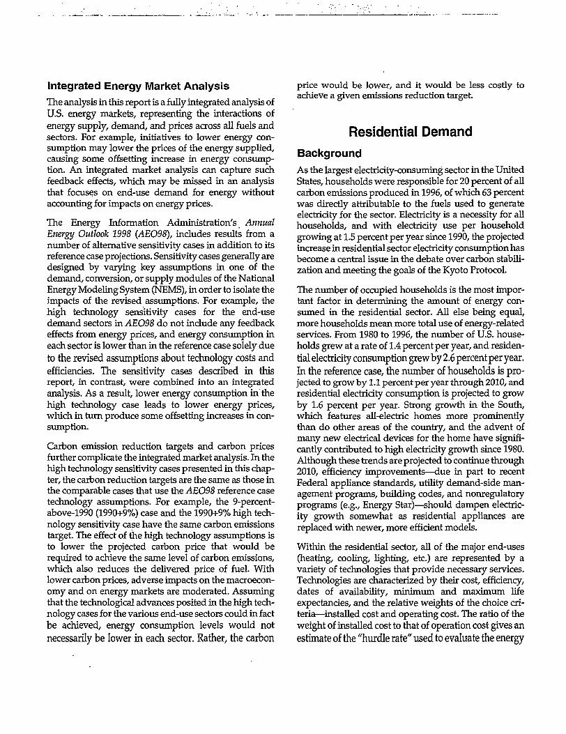
Integrated Energy Market AnalysisThe analysis in this report is a fully integrated analysis ofU.S. energy markets, representing the interactions ofenergy supply, demand, and prices across all fuels andsectors. For example, initiatives to lower energy con-sumption may lower the prices of the energy supplied,causing some offsetting increase in energy consump-tion. An integrated market analysis can capture suchfeedback effects, which may be missed in an analysisthat focuses on end-use demand for energy withoutaccounting for impacts on energy prices.
The Energy Information Administration's AnnualEnergy Outlook 1998 (AEO98), includes results from anumber of alternative sensitivity cases in addition to itsreference case projections. Sensitivity cases generally aredesigned by varying key assumptions in one of thedemand, conversion, or supply modules of the NationalEnergy Modeling System (NEMS), in order to isolate theimpacts of the revised assumptions. For example, thehigh technology sensitivity cases for the end-usedemand sectors in AEO98 do not include any feedbackeffects from energy prices, and energy consumption ineach sector is lower than in the reference case solely dueto the revised assumptions about technology costs and
efficiencies. The sensitivity cases described in thisreport, in contrast, were combined into an integratedanalysis. As a result, lower energy consumption in thehigh technology case leads to lower energy prices,which in turn produce some offsetting increases in con-sumption.
Carbon emission reduction targets and carbon pricesfurther complicate the integrated market analysis. In thehigh technology sensitivity cases presented in this chap-ter, the carbon reduction targets are the same as those inthe comparable cases that use the AEO98 reference casetechnology assumptions. For example, the 9-percent-above-1990 (1990+9%) case and the 1990+9% high tech-nology sensitivity case have the same carbon emissionstarget. The effect of the high technology assumptions isto lower the projected carbon price that would berequired to achieve the same level of carbon emissions,which also reduces the delivered price of fuel. Withlower carbon prices, adverse impacts on the macroecon-omy and on energy markets are moderated. Assumingthat the technological advances posited in the high tech-nology cases for the various end-use sectors could in factbe achieved, energy consumption levels would notnecessarily be lower in each sector. Rather, the carbon
price would be lower, and it would be less costly toachieve a given emissions reduction target.
Residential Demand
BackgroundAs the largest electricity-consuming sector in the UnitedStates, households were responsible for 20 percent of allcarbon emissions produced in 1996, of which 63 percentwas directly attributable to the fuels used to generateelectricity for the sector. Electricity is a necessity for allhouseholds, and with electricity use per householdgrowing at 1.5 percent per year since 1990, the projectedincrease in residential sector electricity consumption hasbecome a central issue in the debate over carbon stabili-zation and meeting the goals of the Kyoto Protocol.
The number of occupied households is the most impor-tant factor in determining the amount of energy con-sumed in the residential sector. All else being equal,more households mean more total use of energy-relatedservices. From 1980 to 1996, the number of U.S. house-holds grew at a rate of 1.4 percent per year, and residen-tial electricity consumption grew by 2.6 percent per year.In the reference case, the number of households is pro-jected to grow by 1.1 percent per year through 2010, andresidential electricity consumption is projected to growby 1.6 percent per year. Strong growth in the South,which features all-electric homes more prominentlythan do other areas of the country, and the advent ofmany new electrical devices for the home have signifi-cantly contributed to high electricity growth since 1980.Although these trends are projected to continue through2010, efficiency improvements—due in part to recentFederal appliance standards, utility demand-side man-agement programs, building codes, and nonregulatoryprograms (e.g., Energy Star)—should dampen electric-ity growth somewhat as residential appliances arereplaced with newer, more efficient models.
Within the residential sector, all of the major end-uses(heating, cooling, lighting, etc.) are represented by avariety of technologies that provide necessary services.Technologies are characterized by their cost, efficiency,dates of availability, minimum and maximum lifeexpectancies, and the relative weights of the choice cri-teria—installed cost and operating cost. The ratio of theweight of installed cost to that of operation cost gives anestimate of the "hurdle rate" used to evaluate the energy
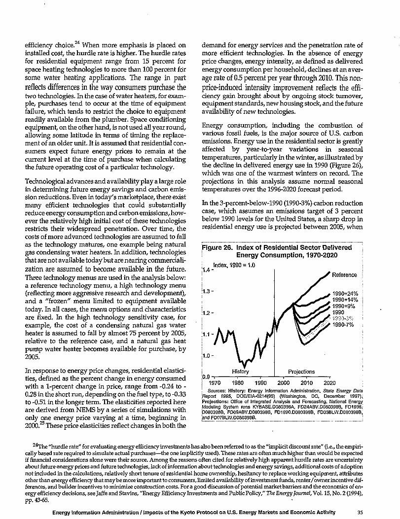
efficiency choice.24 When more emphasis is placed oninstalled cost, the hurdle rate is higher. The hurdle ratesfor residential equipment range from 15 percent forspace heating technologies to more than 100 percent forsome water heating applications. The range in partreflects differences in the way consumers purchase thetwo technologies. In the case of water heaters, for exam-ple, purchases tend to occur at the time of equipmentfailure, which tends to restrict the choice to equipmentreadily available from the plumber. Space conditioningequipment, on the other hand, is not used all year round,allowing some latitude in terms of timing the replace-ment of an older unit. It is assumed that residential con-sumers expect future energy prices to remain at thecurrent level at the time of purchase when calculatingthe future operating cost of a particular technology.
Technological advances and availability play a large rolein determining future energy savings and carbon emis-sion reductions. Even in today's marketplace, there existmany efficient technologies that could substantiallyreduce energy consumption and carbon emissions, how-ever the relatively high initial cost of these technologiesrestricts their widespread penetration. Over time, thecosts of more advanced technologies are assumed to fallas the technology matures, one example being naturalgas condensing water heaters. In addition, technologiesthat are not available today but are nearing commerciali-zation are assumed to become available in the future.Three technology menus are used in the analysis below:a reference technology menu, a high technology menu(reflecting more aggressive research and development),and a "frozen" menu limited to equipment availabletoday. In all cases, the menu options and characteristicsare fixed. In the high technology sensitivity case, forexample, the cost of a condensing natural gas waterheater is assumed to fall by almost 75 percent by 2005,relative to the reference case, and a natural gas heatpump water heater becomes available for purchase, by2005.
In response to energy price changes, residential elastici-ties, defined as the percent change in energy consumedwith a 1-percent change in price, range from -0.24 to -0.28 in the short run, depending on the fuel type, to -0.33to -0.51 in the longer term. The elasticities reported hereare derived from NEMS by a series of simulations withonly one energy price varying at a time, beginning in2000.25 These price elasticities reflect changes in both the
demand for energy services and the penetration rate ofmore efficient technologies. In the absence of energyprice changes, energy intensity, as defined as deliveredenergy consumption per household, declines at an aver-age rate of 0.5 percent per year through 2010. This non-price-induced intensity improvement reflects the effi-ciency gain brought about by ongoing stock turnover,equipment standards, new housing stock, and the futureavailability of new technologies.
Energy consumption, including the combustion ofvarious fossil fuels, is the major source of U.S. carbonemissions. Energy use in the residential sector is greatlyaffected by year-to-year variations in seasonaltemperatures, particularly in the winter, as illustrated bythe decline in delivered energy use in 1990 (Figure 26),which was one of the warmest winters on record. Theprojections in this analysis assume normal seasonaltemperatures over the 1996-2020 forecast period.
In the 3-percent-below-1990 (1990-3%) carbon reductioncase, which assumes an emissions target of 3 percentbelow 1990 levels for the United States, a sharp drop inresidential energy use is projected between 2005, when
Figure 26. Index of Residential Sector DeliveredEnergy Consumption, 1970-2020
Index, 1990 = 1.0
Reference
1990+24%1990+14%1990+9%19901850-3%1990-7%
1.4-
1.3-
1.2-
1.1-
1.0-
IO.9-r1970 1980 1990 2000 2010 2020Sources: History: Energy Information Administration, State Energy Data
Report 1995, DOE/EIA-0214(95) (Washington, DC, December 1997)Projections: Office of Integrated Analysis and Forecasting, National EnergyModeling System runs KYBASE.D080398A, FD24ABV.D080398B, FD1998.D080398B, FD09ABV.D080398B, FD1990.D080398B, FD03BLW.D080398B,'and FD07BLW.D080398B.
2^The "hurdle rate" for evaluating energy efficiency investments has also been referred to as the "implicit discount rate" (i.e., the empiri-cally based rate required to simulate actual purchases—the one implicitly used). These rates are often much higher than would be expectedif financial considerations alone were their source. Among the reasons often cited for relatively high apparent hurdle rates are uncertaintyabout future energy prices and future technologies, lack of information about technologies and energy savings, additional costs of adoptionnot included in the calculations, relatively short tenure of residential home ownership, hesitancy to replace working equipment, attributesother than energy efficiency that maybe more important to consumers, limited availability of investment funds, renter/owner incentive dif-ferences, and builder incentives to minimize construction costs. For a good discussion of potential market barriers and the economics of en-ergy efficiency decisions, see Jaffe and Stavins, "Energy Efficiency Investments and Public Policy," The Energy Journal, Vol. 15, No. 2 (1994),pp. 43-65.
Energy Information Administration / Impacts of the Kyoto Protocol on U.S. Energy Markets and Economic Activity 35

the target is implemented, and 2010 (Figure 26).However, the projected decline is nearly identical to thatseen historically from 1978 to 1983, in terms of bothconsumption and intensity (Figure 27). Housing starts, amajor predictor of residential energy use, fell from 2.02million units in 1978 to 1.062 million in 1982.26 The dropin housing starts was tied directly to mortgage rates,which increased from 9.6 percent in 1978 to over 16percent in 1981-1982. In addition, real energy prices tothe residential sector increased by 87 percent from 1978to 1982, similar to the 82-percent real price increaseprojected in the 1990-3% case. In the carbon reductioncases, delivered energy consumption in the residentialsector never reaches its 1990 level, which has been usedas a benchmark in setting carbon reduction targets.Given the uncertainty regarding technology andconsumer behavior in a high-price energy world,additional sensitivities are examined here to analyze theeffects of variations in the level of optimism associatedwith assumptions about both technology advances andconsumer responsiveness.
Figure 27. Index of Residential Sector Delivered jEnergy Intensity, 1970-2020 j
Index, 1996=1.0
History Projections
Reference
1990+24%1990+9%1990-3%
0.7-r1970 1980 1990 2000 2010 2020Sources: History: Energy Information Administration, State Energy Data
Report 1995, DOE/EIA-0214(95) (Washington, DC, December 1997) and DataResources "Incorporated. Projections: Office of Integrated Analysis andForecasting, National Energy Modeling System runs KYBASE.D080398A;FD24ABV.D080398B, FD09ABV.D080398B, and FD03BLW.D080398B. . j
Carbon Reduction CasesCarbon emissions associated with electricity generationare the largest component of emissions from theresidential sector, in terms of both the levels andprojected growth in the reference case, and in termsof the projected declines in the carbon reduction cases.In the reference case, which does not include theKyoto Protocol, 98 percent of the projected increasein residential sector carbon emissions by 2010 resultsfrom increasing electricity use and the fuels used for
electricity generation. In the 1990+9% case, 87 percent ofthe sector's decline in carbon emissions is related toreduced electricity demand and changes in electricitygeneration (Figure 28). The following discussion focuseson the results of three carbon reduction cases—1990-3%,1990+9%, and 24-percent-above-1990 (1990+24%)—inwhich carbon emissions, averaged across all energysectors, reach targeted levels relative to 1990 in the 2008-2012 period.
'Figure 28. Residential Sector Carbon Emissions,1990,1996, and 2010
5250 -
! 0 0 -
[150-
hoo-
5 0 -
Million Metric Tons
History Projections for 2010
•Electr ic
•Eton-Electric
OTOTO
CM
+OTOTO
+OTOTO
OTOTO
s «TOTO
TOTO
Note: Electricity emissions are from the fossil fuels used to generatethe electricity used in this sector. j! Sources: History: Energy Information Administration, Emissions ofGreenhouse Gases in the United States 1996, DOE/EIA-0573(96) (Washington]DC, October 1997). Projections: Office of Integrated Analysis and Forecasting;National Energy Modeling System runs KYBASE.D080398A, FD24ABV;'D080398B, FD1998.D080398B, FD09ABV.D080398B, FD1990.D08O398BJFD03BLW.D080398B, and FD07BLW.D080398B.
Although the use of electricity contributes most to theprojected growth in emissions in the residential sector,natural gas consumption, which emits relatively lowlevels of carbon per Btu burned compared with coal (themajor fuel used to generate electricity), is projected toremain the most important fuel in the sector asmeasured by delivered energy. Figure 29 shows deliv-ered energy consumption by major fuel as well as thelosses associated with electricity generation. On a deliv-ered basis, natural gas use is projected to decrease themost in the three carbon reduction cases by 2010. Rela-tive to the projected level of consumption in the refer-ence case in 2010, delivered energy consumption isprojected to be 10 percent lower in the 1990+9% case andelectricity-related losses 22 percent lower. Of the 2.0quadrillion Btu savings in electricity-related losses in2010 in the 1990+9% case, 43 percent (0.9 quadrillionBtu) can be attributed to reduced electricity demand inthe residential sector. The remaining 1.1 quadrillion Btu(57 percent) of the savings in electricity-related lossescomes from efficiency gains and/or fuel switching for
^The long-run elasticities reflect the effects of altered prices after 20 years for the last year of the forecast, 2020.26U.S. Bureau of the Census, Construction Reports, series C20.

Figure 29. Delivered Energy Consumption in theResidential Sector by Major Fuel, 1970,1980,1996, and 2010
Quadrillion Btu1 2 "•Natural Gas •Electricity •Petrolsurn •Electricity-
Related Losses
Projections for 2010
oa>
ooo^-
<OCOCD
IDUc
(D
5
CM
OO>
cn
oCO
Sources: History: Energy Information Administration, State Energy Datafteport 199S, DOE/EIA-0214(95) (Washington, DC, December 1997).;Projections: Office of Integrated Analysis and Forecasting, National EnergyModeling System runs KYBASE.D080398A, FD24ABV.D080398B, FD09ABV.D080398B,andFD03BLW.D080398B. !
electricity generation. Thus, changes in electricitysupply, absent any major technological or behavioralchanges in residential end use over the next 12 years, arethe key to controlling carbon emissions for theresidential sector.
Energy is used in the residential sector to provide anumber of different services, which vary in end-useintensity (energy consumption per household) (Figure30). Space conditioning (which includes heating,cooling, and ventilation) is clearly the most energy-intensive end use in the sector, and it accounts for mostof the direct use of fossil fuels. "White goods" (whichinclude refrigerators, freezers, dishwashers, clotheswashers and dryers, and stoves), lighting, and otheruses are almost entirely powered by electricity and,therefore, are responsible for most of the electricity-related losses.
In the reference case, most of the projected growth inresidential energy consumption between 1996 and 2010comes from increasing use of miscellaneous electricdevices, such as personal computers and home securitysystems (Figure 31). The rate at which energy consump-tion changes over time depends on factors such asequipment turnover rates, ability to control unit opera-tion (thermostatic controls), energy prices, householdsize (people per house), housing unit size (square feet),and the efficiency of newly purchased appliances. Stockturnover can provide drastic reductions in energy inten-sity, even without future gains in appliance efficiency.On average, a new refrigerator purchased in 1995 used
Figure 30. Residential Sector Energy Use perHousehold, 1996
Source: Office of Integrated Analysis and Forecasting, National EnergyModeling System run KYBASE.D080398A.
100-
8 0 -
60 -
40 -
20 -
Million Btu per Household
I Electricity-Related Losses
•Direct Use
Space Water White
Conditioning Heating Goods
Lighting Other Uses
Figure 31. Average Projected Annual Growth inResidential Sector Energy Consumptionby End Use, 1996-2010
5 -Percent per Year
•Reference •1990+24% •1990+9% •i9?D-?>%
Space Water WhiteConditioning Heating Goods
Lighting Other Uses
Source: Office of Integrated Analysis and Forecasting, National EnergyModeling System runs KYBASE.D080398A, FD24ABV.D080398B, FD09ABV.D080398B, and FD03BLW.D080398B..
62 percent less electricity than one purchased 20 yearsearlier. Conversely, slow stock turnover can limit therole of energy efficiency gains in the future. Equipmentpurchased in the 1990s that lasts 20 years or more willnot be eligible for replacement until after 2010.
With the exception of white goods, increases in totalenergy consumption for all the major residential energyservices are projected from 1996 to 2010 in the referencecase. The negative growth in total energy consumptionfor white goods results from a decline in energy use for
^Association of Home Appliance Manufacturers, Fact Book 1996.
Energy Information Administration / Impacts of the Kyoto Protocol on U.S. Energy Markets and Economic Activity 37

refrigeration, as aggressive Federal efficiency stand-ards taking effect in 1993 and 2001 reduce the amountof energy needed to provide the same level of service. Inthe carbon reduction cases, increasing energy prices actto reduce the growth in energy consumption for allmajor services relative to their growth in the referencecase. In the absence of mandatory standards, residentialconsumers traditionally have been reluctant to purchasehighly efficient appliances. However, faced with thehigher energy prices projected in the carbon reductioncases, it is expected that consumers will respond bypurchasing more efficient appliances (Table 4). The ex-tent of consumer response and its impact on averageequipment efficiencies would also depend on the pur-chase price of the new equipment (the initial investmentrequired).
Table 4. Change in Projected Average Efficienciesof Newly Purchased ResidentialEquipment in Carbon Reduction CasesRelative to the Reference Case, 2010(Percent)
Technology 11990+24% [ 1990+9% | 1990-3%Air-Source Heat Pump 1.3 3.6 5.7
Electric Water Heater 0.3 2.4 13.6Natural Gas Water H e a t e r . . 1.1 3.7 4.8 I
! Building Shell 1.0 3^3 5.5 I
I Source: Office of Integrated Analysis and Forecasting, National Energy Mod-jeling System runs KYBASE.D080398A, FD24ABV.D080398B, FD09ABV.'D080398B, and FD03BLW.D080398B. j
In the reference case, the real (inflation-adjusted) pricesof electricity and natural gas to residential consumersare projected to decline between 1996 and 2010 (Figure32), by 8 and 10 percent, respectively. The outlook forprices in the carbon reduction cases, however, is muchdifferent. Without major changes in energy policy,technology, or consumer response, prices to theresidential sector are expected to be as much as 94percent higher in 2010 in the 1990-3% case. In responseto the higher prices, total residential energy consump-tion is projected to decline by more than 20 percent by2010 in the 1990-3% case.
The factors that contribute to lower consumptioninclude behavioral responses, such as adjusting thethermostat or turning off the lights when leaving theroom, and, to a lesser extent, the acquisition of moreefficient appliances. The rate of improvement in averageappliance efficiency is constrained by the rate of stockturnover. For example, it is not uncommon for majorenergy-using appliances, such as furnaces, to last for 30years or more. More immediate responses to higher
energy prices can be achieved through retrofits toimprove the thermal efficiency of building shells.During the energy price shocks of the 1970s, forexample, homeowners increased insulation levelssubstantially,29 with the immediate effect of conservingenergy and lowering energy bills. The potential forsimilar improvement between 1996 and 2010 is reduced,given the improvements already made.
Figure 32. Index of Residential Sector Energyj Prices, 1970,1980,1996, and 2010S Index, 1996=1.0
1.8-
1.6-
J 1 . 4 -1.2-
1.0-i
;o.8-
;o.6-
j o . 4 -:o.2-
o.o
•Natural Gas
History
[Electricity •Petroleum
Projections for 2010
1970 1980 1996 Reference 1990+24%
1990+9%
1990-3%
i Sources: History: Energy Information Administration, State Energy Price and•Expenditure Report 1994, DOE/EIA-0376(94) (Washington, DC, June 1997)'Projections: Office of Integrated Analysis and Forecasting, National Energy!Modeling System runs KYBASE.D080398A, FD24ABV.D080398B, FD09ABV^D080398B, and FD03BLW.D080398B.
Sensitivity CasesHigh and Low Technology. Technology improvementsover time can take the form of increased efficiency,decreased cost, or both. To examine the effects ofassumptions about the rate at which technologies willimprove in the future, two sets of sensitivity cases wereanalyzed. The low technology sensitivity cases assumethat none of the improvements assumed in the referencecase will occur. In other words, future technologies areassumed to be "frozen" at their 1998 cost and efficiencylevels. Technological improvement occurs in this case asolder units are retired and are replaced with 1998 tech-nologies. Engineering technology experts were con-sulted to develop the high technology case, whichassumes more rapid advances than those in the refer-ence case, due to research and development (Table 5).30
In the high technology case, for example, the efficiencyof the best available natural gas water heater isassumed to improve by 63 percent over the 1998 level by2015, and the cost is assumed to decline by 15 percent,
28These standards represent updates to previous standards authorized by the National Appliance Energy Conservation Act of 1987.29U.S. Department of Energy, Progress in Residential Retrofit, Based on Owens-Corning Marketing Research.30Energy Information Administration, Technology Forecast Updates—Residential and Commercial Building Technologies, Draft Report (Ar-
thur D. Little, Inc., June 1998).
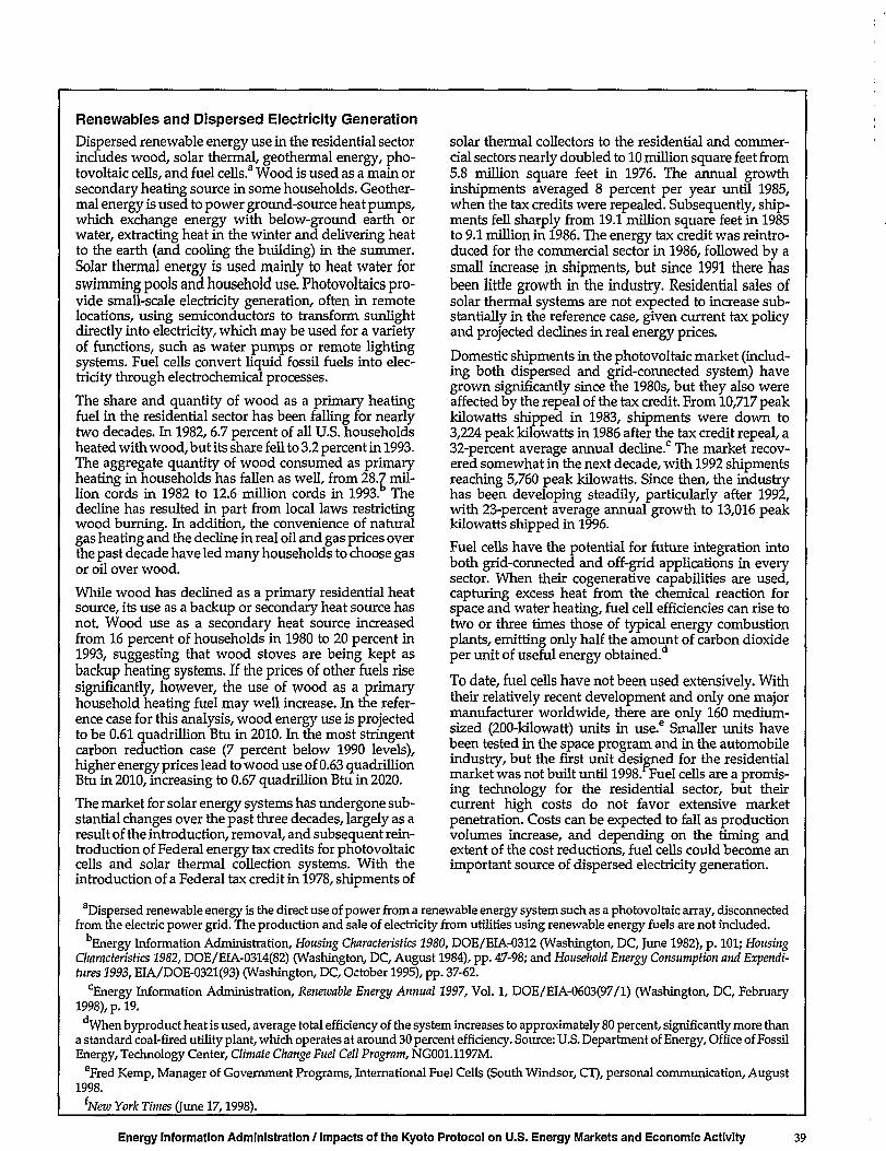
Renewables and Dispersed Electricity GenerationDispersed renewable energy use in the residential sectorincludes wood, solar thermal, geothermal energy, pho-tovoltaic cells, and fuel cells.a Wood is used as a main orsecondary heating source in some households. Geother-mal energy is used to power ground-source heat pumps,which exchange energy with below-ground earth orwater, extracting heat in the winter and delivering heatto the earth (and cooling the building) in the summer.Solar thermal energy is used mainly to heat water forswimming pools and household use. Photovoltaics pro-vide small-scale electricity generation, often in remotelocations, using semiconductors to transform sunlightdirectly into electricity, which may be used for a varietyof functions, such as water pumps or remote lightingsystems. Fuel cells convert liquid fossil fuels into elec-tricity through electrochemical processes.
The share and quantity of wood as a primary heatingfuel in the residential sector has been falling for nearlytwo decades. In 1982,6.7 percent of all U.S. householdsheated with wood, but its share fell to 3.2 percent in 1993.The aggregate quantity of wood consumed as primaryheating in households has fallen as well, from 28.7 mil-lion cords in 1982 to 12.6 million cords in 1993.b Thedecline has resulted in part from local laws restrictingwood burning. In addition, the convenience of naturalgas heating and the decline in real oil and gas prices overthe past decade have led many households to choose gasor oil over wood.
While wood has declined as a primary residential heatsource, its use as a backup or secondary heat source hasnot. Wood use as a secondary heat source increasedfrom 16 percent of households in 1980 to 20 percent in1993, suggesting that wood stoves are being kept asbackup heating systems. If the prices of other fuels risesignificantly, however, the use of wood as a primaryhousehold heating fuel may well increase. In the refer-ence case for this analysis, wood energy use is projectedto be 0.61 quadrillion Btu in 2010. In the most stringentcarbon reduction case (7 percent below 1990 levels),higher energy prices lead to wood use of 0.63 quadrillionBtu in 2010, increasing to 0.67 quadrillion Btu in 2020.
The market for solar energy systems has undergone sub-stantial changes over the past three decades, largely as aresult of the introduction, removal, and subsequent rein-troduction of Federal energy tax credits for photovoltaiccells and solar thermal collection systems. With theintroduction of a Federal tax credit in 1978, shipments of
solar thermal collectors to the residential and commer-cial sectors nearly doubled to 10 million square feet from5.8 million square feet in 1976. The annual growthinshipments averaged 8 percent per year until 1985,when the tax credits were repealed. Subsequently, ship-ments fell sharply from 19.1 million square feet in 1985to 9.1 million in 1986. The energy tax credit was reintro-duced for the commercial sector in 1986, followed by asmall increase in shipments, but since 1991 there hasbeen little growth in the industry. Residential sales ofsolar thermal systems are not expected to increase sub-stantially in the reference case, given current tax policyand projected declines in real energy prices.
Domestic shipments in the photovoltaic market (includ-ing both dispersed and grid-connected system) havegrown significantly since the 1980s, but they also wereaffected by the repeal of the tax credit. From 10,717 peakkilowatts shipped in 1983, shipments were down to3,224 peak kilowatts in 1986 after the tax credit repeal, a32-percent average annual decline.0 The market recov-ered somewhat in the next decade, with 1992 shipmentsreaching 5,760 peak kilowatts. Since then, the industryhas been developing steadily, particularly after 1992,with 23-percent average annual growth to 13,016 peakkilowatts shipped in 1996.
Fuel cells have the potential for future integration intoboth grid-connected and off-grid applications in everysector. When their cogenerative capabilities are used,capturing excess heat from the chemical reaction forspace and water heating, fuel cell efficiencies can rise totwo or three times those of typical energy combustionplants, emitting only half the amount of carbon dioxideper unit of useful energy obtained.d
To date, fuel cells have not been used extensively. Withtheir relatively recent development and only one majormanufacturer worldwide, there are only 160 medium-sized (200-kilowatt) units in use.6 Smaller units havebeen tested in the space program and in the automobileindustry, but the first unit designed for the residentialmarket was not built until 1998. Fuel cells are a promis-ing technology for the residential sector, but theircurrent high costs do not favor extensive marketpenetration. Costs can be expected to fall as productionvolumes increase, and depending on the timing andextent of the cost reductions, fuel cells could become animportant source of dispersed electricity generation.
aDispersed renewable energy is the direct use of power from a renewable energy system such as a photovoltaic array, disconnectedfrom the electric power grid. The production and sale of electricity from utilities using renewable energy fuels are not included.
bEnergy Information Administration, Housing Characteristics 1980, DOE/EIA-0312 (Washington, DC, June 1982), p . 101; HousingCharacteristics 1982, DOE/EIA-0314(82) (Washington, DC, August 1984), pp. 47-98; and Household Energy Consumption and Expendi-tures 1993, EIA/DOE-0321(93) (Washington, DC, October 1995), pp. 37-62.
cEnergy Information Administration, Renewable Energy Annual 1997, Vol. 1, DOE/EIA-0603(97/1) (Washington, DC, February1998), p. 19.
When byproduct heat is used, average total efficiency of the system increases to approximately 80 percent, significantly more thana standard coal-fired utility plant, which operates at around 30 percent efficiency. Source: U.S. Department of Energy, Office of FossilEnergy, Technology Center, Climate Change Fuel Cell Program, NG001.1197M.
eFred Kemp, Manager of Government Programs, International Fuel Cells (South Windsor, CT), personal communication, August1998.
{New YorkTimes June 17,1998).
Energy Information Administration / Impacts of the Kyoto Protocol on U.S. Energy Markets and Economic Activity 39
Table 5. Cost and Efficiency2015(1998 Values = 1.00)
Technology
Indexes of Best Available Technologies
Cost
1990+9%Low
Technology 1990+9%
1990+9%High
Technology
for Selected Residential Appliances,
Efficiency
1990+9%Low
Technology 1990+9%
1990+9%High
Technology
! Air-Source Heat Pump
| Ground-Source Heat Pump.
i Natural Gas Heat Pump . . .
! Natural Gas Water Heater..
Solar Water Heater
; Electric Water Heater
1.00
1.00
1.00
1.00
1.00
1.00
0.99
0.86
0.81
0.76
1.00
1.00
0.980.560.750.850.730.73
1.00
1.00
1.00
1.00
1.00
1.00
1.09
1.05
1.00
1.00
1.00
1.04
1.18
1.08
1.00
1.63
1.67
1.17
; Source: Office of Integrated Analysis and Forecasting, National Energy Modeling System runs FREEZE09.D080798A, FD09ABV.D080398B, andHITECH09.D080698A, computed from Technology Forecast Updates—Residential and Commercial Building Technologies, Draft Report (Arthur D. Little, Inc., June1998).
while ground-source heat pumps, which do not realizemuch gain in efficiency, are assumed to decline in costby 44 percent in the high technology case by 2015.
Ground-source heat pumps, which draw stored heatfrom the ground beneath the frost line, provide anefficient and comfortable (in terms of delivered heat)alternative to the more common air-source heat pumps.The cost of the unit and the placement of the groundloop have been major barriers to wide market accep-tance, however. Different levels of stocks of ground-source heat pumps are projected in the reference case,the 1990+9% carbon reduction case, and the 1990+9%case low and high technology cases (Figure 33). Giventhat significant market acceptance is seen only in thehigh technology case, it can be concluded that tine costsassociated with the technology restrict its acceptance.Space heating technologies, in general, have the lowesthurdle rates (15 percent) of all residential appliances,primarily because of the large energy costs of home heat-ing, relative to other energy-using services.
Figure 34 shows that improvements in technology canindeed dampen the impact carbon restrictions have onresidential energy prices. Given the amount of timeneeded for technology to penetrate the market, onewould expect that over a longer period of time, theprices in the high technology sensitivity would fallrelative to the other cases. After 2008, prices in the hightechnology sensitivity begin to fall, as reduced energydemand caused by more efficient technology penetrat-ing the market begin to make an impact. Relative to theprice in the 1990+9% case, the composite real residentialenergy price in 2010 is 11 percent less in the high technol-ogy case. Conversely, if technology were frozen at thelevel available in 1998,2010 prices are expected to be 17percent higher than the 1990+9% case, indicating thatenergy efficiency plays a significant role in the caseswith reference technology assumptions.
Energy fuel expenditures are a good indication of thesuccess that technological advancement achieves in
Figure 33. Projected Stocks of Ground-Source|| Heat Pumps, 1995-2020! Million Units16-! 1990+9% High TechnologyJ
k-• 3 -
H -
1990+9%.
Reference_ — • —
1990+9% Low Technology
Source: Office of Integrated Analysis and Forecasting, National EnergyModeling System runs KYBASE.D080398A, FREEZE09.D080798A, FD09ABV.
Figure 34. Average Residential Sector EnergyPrices, 1995-2020
1995 2000 2005 2010 2015 2020
£5-
2 0 -
1 5 -
1996 Dollars per Million Btu
1990+9%Low
Technology1990+9%
Reference
1990+9%High
Technology
Projections
1970 1980 1990 2000 2010 2020,
Sources: History: Energy Information Administration, State Energy Price andExpenditure Report 1994, DOE/EIA-0376(94) (Washington, DC, June 1997),Projections: Office of Integrated Analysis and Forecasting, National EnergyModeling System runs KYBASE.D080398A, FREEZE09.D080798A, FD09ABVJD080398B, and HITECH09.D080698A.

lessening the impact on the consumer in a carbon-restricted environment. Figure 35 details residentialsector energy expenditures for the 1990+9% case andtechnology sensitivities. For the high technologysensitivity, energy expenditures in 2020 are 23 percentless than those realized in the 1990+9% case, savingconsumers over $440 billion from 2008 to 2020.
Figure 35. Projected Energy Expenditures in theI Residential Sector, 1995-2020
3 0 0 -Billion 1996 Dollars
1990+9%
990+9% High Technology
Reference
J 1 0 0 -
5 0 -
1995 2000 2005 2010 2015 2020J
| Source: Office of Integrated Analysis and Forecasting, National EnergyModeling System runs KYBASE.D080398A, FREEZE09.D080798A, FD09ABV;" O98B, and HITECH09.D080698A.
Increased Consumer Response. Residential energyconsumers have traditionally been reluctant to invest inenergy efficiency, even with ample financial benefits.Many market barriers tend to create what are known ashigh hurdle rates for consumer investments in energyefficiency. As of 1993, 35 percent of all homes wereoccupied by renters,31 most of whom were responsiblefor paying energy bills but not for purchasing majorenergy-consuming appliances. Such households tend tobuy the least expensive equipment on the market, whichalso tends to be the least energy-efficient. The samereasoning can be applied to many newly constructedhomes as well, because the builders, not the occupants,are tasked with equipping them with most of the majorenergy-using appliances. Other barriers includeequipment availability (e.g., whether plumbingcontractors have high-efficiency water heaters availablewhen they make service calls) and lack of information.
To examine the effects that lower hurdle rates couldhave on both energy prices and expenditures in the car-bon reduction cases, and at the same time differentiatethose effects from the effects of technological advances,
an increased consumer response sensitivity case wasanalyzed. This sensitivity case includes assumptions oflower discount rates, higher short-run elasticities ofdemand, greater inclination to change fuels when pur-chasing equipment, and lower growth in miscellaneouselectricity use.'32
Impacts of Increased Consumer Response andAdvanced Technology. In order to gauge the impact ofassumptions regarding technological advancement andconsumer behavior with respect to delivered energyconsumption, sensitivity cases were analyzed relative tothe 1990+9% case where delivered energy prices werethe same across all cases. These cases serve to isolate theimpact of each of the key variables separately, and tounderstand the impact of implementing the sensitivitiessimultaneously. This section evaluates the relativeimpact that each of these concepts could have on futureenergy intensity at a price level realized in the 1990+9%case.
Changes in technological development and the valueresidential consumers place on energy related issues cansignificantly affect the pattern of energy consump-tion—and carbon emissions—in the future. The avail-ability of high-efficiency technologies in itself does notguarantee increased energy efficiency. Without the will-ingness of consumers to purchase the more efficientproducts, which usually cost significantly more, tech-nology may not have much of an impact on futureenergy consumption patterns. Conversely, in a worldwhere energy conservation was of paramount concernto energy consumers, yet at the same time high-efficiency products were unavailable, future energy con-sumption patterns would probably not be greatlyaffected either.
Given the detailed nature regarding technologicaldevelopment and consumer choice with regards to dif-ferent technologies, it is important to analyze the resultsat the technology level, as well as the overall level. Withnearly 40 million households (38 percent) using electricwater heaters in 1995, and given the relatively highintensity associated with using electric water heaters,the projected impact of increased energy efficiency canhave a large impact on future electricity use for this serv-ice. Electric resistance water heaters have traditionallyexhibited slow growth in energy efficiency. In fact, thehighest efficiency unit available today is not likely to seeany efficiency improvement due to thermal limits anddiminishing returns on controlling heat loss.33 Thisimplies that future gains in efficiency for electric water
31Energy Information Administration, Housing Characteristics 1993.32Assumptions include lowering hurdle rates to 15 percent real, increasing the price sensitivity parameters to switch fuels, increasing
short-run price elasticities from -0.25 to -0.40, and decreasing miscellaneous electricity penetration.33Energy Information Administration, Technology Forecast Updates—Residential and Commercial Building Technologies, Draft Report (Ar-
thur D. Little, Inc., June 1998).
Energy Information Administration / Impacts of the Kyoto Protocol on U.S. Energy Markets and Economic Activity 41
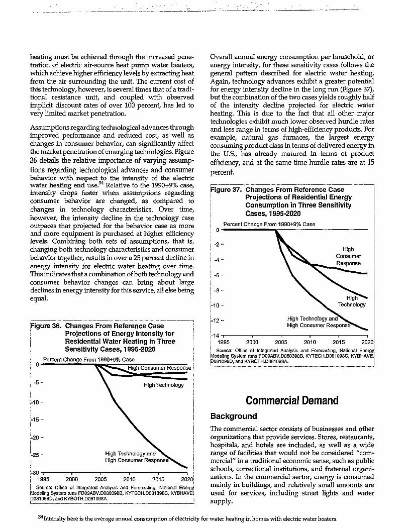
heating must be achieved through the increased pene-tration of electric air-source heat pump water heaters,which achieve higher efficiency levels by extracting heatfrom the air surrounding the unit. The current cost ofthis technology, however, is several times that of a tradi-tional resistance unit, and coupled with observedimplicit discount rates of over 100 percent, has led tovery limited market penetration.
Assumptions regarding technological advances throughimproved performance and reduced cost, as well aschanges in consumer behavior, can significantly affectthe market penetration of emerging technologies. Figure36 details the relative importance of varying assump-tions regarding technological advances and consumerbehavior with respect to the intensity of the electricwater heating end use.34 Relative to the 1990+9% case,intensity drops faster when assumptions regardingconsumer behavior are changed, as compared tochanges in technology characteristics. Over time,however, the intensity decline in the technology caseoutpaces that projected for the behavior case as moreand more equipment is purchased at higher efficiencylevels. Combining both sets of assumptions, that is,changing both technology characteristics and consumerbehavior together, results in over a 25 percent decline inenergy intensity for electric water heating over time.This indicates that a combination of both technology andconsumer behavior changes can bring about largedeclines in energy intensity for this service, all else beingequal.
Figure 36. Changes From Reference CaseProjections of Energy Intensity forResidential Water Heating in ThreeSensitivity Cases, 1995-2020
Percent Change From 1990+9% Case
- 5 -
[-10 -
-15-
- 2 0 -
i-25- High Technology andHigh Consumer Response*
i-30-r-1995 2000 2005 2010 2015 2020;
I Source: Office of Integrated Analysis and Forecasting, National EnergyModeling System runs FD09ABV.D080398B, KYTECH.D081098C, KYBHAVE.D081098D, and KYBOTH.D081098A.
Overall annual energy consumption per household, orenergy intensity, for these sensitivity cases follows thegeneral pattern described for electric water heating.Again, technology advances exhibit a greater potentialfor energy intensity decline in the long run (Figure 37),but the combination of the two cases yields roughly halfof the intensity decline projected for electric waterheating. This is due to the fact that all other majortechnologies exhibit much lower observed hurdle ratesand less range in terms of high-efficiency products. Forexample, natural gas furnaces, the largest energyconsuming product class in terms of delivered energy inthe U.S., has already matured in terms of productefficiency, and at the same time hurdle rates are at 15percent.
Figure 37. Changes From Reference CaseProjections of Residential EnergyConsumption in Three SensitivityCases, 1995-2020
Percent Change From 1990+9% Case
- 2 -
-4 -
- 6 -
- 8 -
• 1 0 -
- 1 2 -
HighConsumerResponse
High Technology andHigh Consumer Response*
-14 T -
1995 2000 2005 2010 2015 2020
Source: Office of Integrated Analysis and Forecasting, National EnergyModeling System runs FD09ABV.D080398B, KYTECH.D081098C, KYBHAVEJ
081098D, and KYBOTH.D081098A. I
Commercial DemandBackground
The commercial sector consists of businesses and otherorganizations that provide services. Stores, restaurants,hospitals, and hotels are included, as well as a widerange of facilities that would not be considered "com-mercial" in a traditional economic sense, such as publicschools, correctional institutions, and fraternal organi-zations. In the commercial sector, energy is consumedmainly in buildings, and relatively small amounts areused for services, including street lights and watersupply.
^Intensity here is the average annual consumption of electricity for water heating in homes with electric water heaters.

The commercial sector is currently the smallest of thefour demand sectors in terms of energy use, accountingfor 11 percent of delivered energy demand in 1996. Thecommercial sector is also responsible for fewer carbonemissions than the other sectors, emitting 230 millionmetric tons, or 16 percent of total U.S. carbon emissions,in 1996. The sector has a larger share of emissions thanits share of energy use because of the importance of com-mercial electricity use. The emissions associated withelectricity-related losses are included in the calculationof emissions from electricity use.
Several factors determine energy use and, consequently,carbon emissions in the commercial sector. One of themost important is floorspace. Building location, age, andtype of activity also affect commercial energy use. Cur-rently, total commercial floorspace in the United Statesexceeds the area of the State of Delaware and amounts toabout 200 square feet for every U.S. resident. Mercantile(retail and wholesale stores) and service businesses arethe most common type of commercial buildings, andoffices and warehouses are also common.'"35
Because of the relatively long lives of buildings, the char-acteristics of the stock of commercial floorspace changeslowly. Over half of the commercial buildings in theUnited States were built before 1970, and the referencecase used for this analysis projects that total commercialfloorspace will grow at about the same rate as popula-tion, 0.8 percent annually, through 2020. This limits theeffects that new, more efficient building practices canachieve in the near term, but as time passes and buildingstock "turnover" occurs, current and future buildingpractices will have a greater effect on commercial energyuse.
The composition of end-use services is another determi-nant of the amount of energy consumed and the type offuel used. The majority of energy use in the commercialsector is for lighting, space heating, cooling, and waterheating. In addition, the proliferation of new electricaldevices, including telecommunications equipment, per-sonal computers, and other office equipment, is spur-ring growth in electricity use. Electricity use currentlyaccounts for 45 percent of delivered energy consump-tion in the sector, and that share is projected to grow toabout 48 percent by 2010 in the reference case.
Consideration of end-use services leads to anotherdetermining factor in commercial energy consump-tion—the effects of turnover and change in end-use tech-nologies. The stock of installed equipment changes withnormal turnover as old, worn-out equipment is replacedand new buildings are outfitted with newer versionsof equipment that tend to be more energy-efficient.
Equipment with even greater energy efficiency isexpected to be available to commercial consumers in thefuture. Energy prices have both short-term and long-term effects on commercial energy use. Fuel prices influ-ence energy demand in the short run by affecting the useof installed equipment and in the long run by affectingthe stock of installed equipment.
Legislated efficiency standards also affect energy use, byimposing a minimum level of efficiency for purchases ofseveral types of equipment used in the commercial sec-tor. Two mandates currently affect commercial appli-ances: the National Energy Policy Act of 1992 (P.L. 102-486, Title II, Subtitle C, Section 342), which specificallytargets larger-scale commercial equipment and fluores-cent lighting, and the National Appliance Energy Con-servation Amendments (NAECA), which affectcommercial buildings that install smaller residential-style equipment. Examples include standards for heatpumps, air conditioning units, boilers, furnaces, waterheating equipment, and fluorescent lighting.
Effects of Technology Availabilityand ChoiceThe degree to which energy-efficient equipment canaffect energy consumption, and in turn carbon emis-sions, in the commercial sector is limited by the level ofefficiency available to commercial consumers and therate at which more efficient equipment is purchased.Technologies for all the major end uses (lighting, heat-ing, cooling, water heating, etc.) are defined by theirinstalled cost, operating cost, efficiency, average usefullife, and first and last dates of availability. Theseparameters are considered, along with fuel prices at thetime of purchase, in the selection of technologies thatprovide end-use services. Commercial consumers arenot assumed to anticipate any future changes in fuelprices when choosing equipment. The commercial sec-tor encompasses a wide variety of buildings, and not allconsumers will have the same requirements and priori-ties when purchasing equipment. Major assumptionsthat take these differences in behavior into account andaffect commercial technology choices are describedbelow.
In making the tradeoffs between equipment cost andequipment efficiency, the purchase behavior of the com-mercial sector is represented by distributing floorspaceover a variety of hurdle rates. Rates of return on invest-ments in energy efficiency (referred to in financial par-lance as "internal rates of return") are required to meetor exceed the hurdle rate. Floorspace is distributed overhurdle rates that range from a low of about 18 percent torates high enough to cause choices to be made solely by
•^General characteristics of the commercial sector provided in the above paragraphs are from Energy Information Administration, ALookat Commercial Buildings in 1995: Characteristics, Energy Consumption, and Energy Expenditures, DOE/EIA-0318(95) (Washington, DC, Sep-tember 1998).
Energy Information Administration / Impacts of the Kyoto Protocol on U.S. Energy Markets and Economic Activity 43
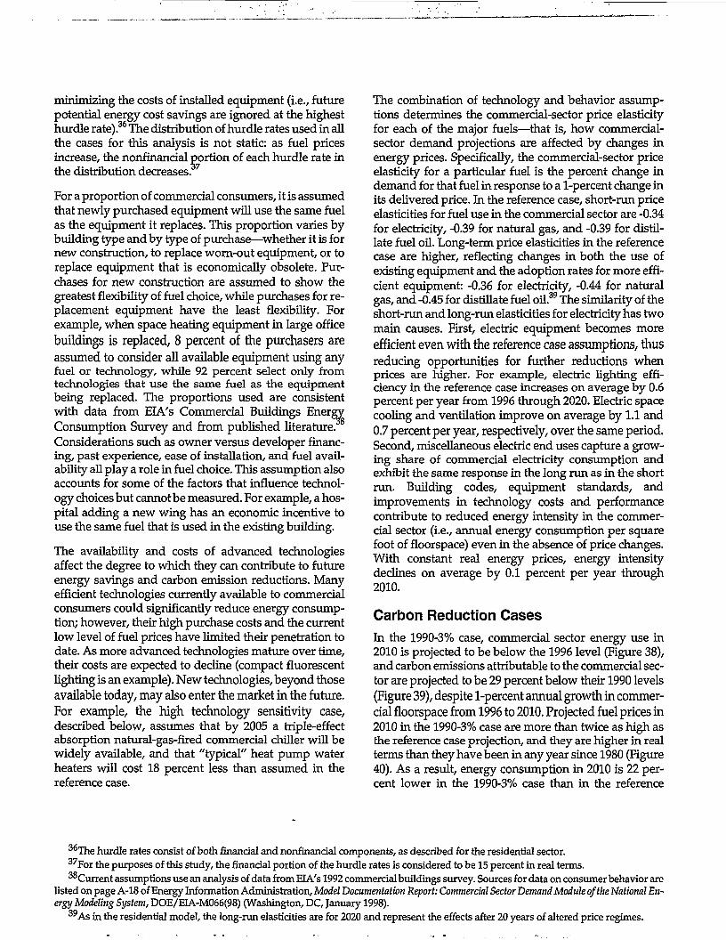
minimizing the costs of installed equipment (i.e., futurepotential energy cost savings are ignored at the highesthurdle rate).36 The distribution of hurdle rates used in allthe cases for this analysis is not static: as fuel pricesincrease, the nonfinancial portion of each hurdle rate inthe distribution decreases.'37
For a proportion of commercial consumers, it is assumedthat newly purchased equipment will use the same fuelas the equipment it replaces. This proportion varies bybuilding type and by type of purchase—whether it is fornew construction, to replace worn-out equipment, or toreplace equipment that is economically obsolete. Pur-chases for new construction are assumed to show thegreatest flexibility of fuel choice, while purchases for re-placement equipment have the least flexibility. Forexample, when space heating equipment in large officebuildings is replaced, 8 percent of the purchasers areassumed to consider all available equipment using anyfuel or technology, while 92 percent select only fromtechnologies that use the same fuel as the equipmentbeing replaced. The proportions used are consistentwith data from EIA's Commercial Buildings EnergyConsumption Survey and from published literature.8
Considerations such as owner versus developer financ-ing, past experience, ease of installation, and fuel avail-ability all play a role in fuel choice. This assumption alsoaccounts for some of the factors that influence technol-ogy choices but cannot be measured. For example, a hos-pital adding a new wing has an economic incentive touse the same fuel that is used in the existing building.
The availability and costs of advanced technologiesaffect the degree to which they can contribute to futureenergy savings and carbon emission reductions. Manyefficient technologies currently available to commercialconsumers could significantly reduce energy consump-tion; however, their high purchase costs and the currentlow level of fuel prices have limited their penetration todate. As more advanced technologies mature over time,their costs are expected to decline (compact fluorescentlighting is an example). New technologies, beyond thoseavailable today, may also enter the market in the future.For example, the high technology sensitivity case,described below, assumes that by 2005 a triple-effectabsorption natural-gas-fired commercial chiller will bewidely available, and that "typical" heat pump waterheaters will cost 18 percent less than assumed in thereference case.
The combination of technology and behavior assump-tions determines the commercial-sector price elasticityfor each of the major fuels—that is, how commercial-sector demand projections are affected by changes inenergy prices. Specifically, the commercial-sector priceelasticity for a particular fuel is the percent change indemand for that fuel in response to a 1-percent change inits delivered price. In the reference case, short-run priceelasticities for fuel use in the commercial sector are -0.34for electricity, -0.39 for natural gas, and -0.39 for distil-late fuel oil. Long-term price elasticities in the referencecase are higher, reflecting changes in both the use ofexisting equipment and the adoption rates for more effi-cient equipment: -0.36 for electricity, -0.44 for naturalgas, and -0.45 for distillate fuel oil.39 The similarity of theshort-run and long-run elasticities for electricity has twomain causes. First, electric equipment becomes moreefficient even with the reference case assumptions, thus
reducing opportunities for further reductions whenprices are higher. For example, electric lighting effi-ciency in the reference case increases on average by 0.6percent per year from 1996 through 2020. Electric spacecooling and ventilation improve on average by 1.1 and0.7 percent per year, respectively, over the same period.Second, miscellaneous electric end uses capture a grow-ing share of commercial electricity consumption andexhibit the same response in the long run as in the shortrun. Building codes, equipment standards, andimprovements in technology costs and performancecontribute to reduced energy intensity in the commer-cial sector (i.e., annual energy consumption per squarefoot of floorspace) even in the absence of price changes.With constant real energy prices, energy intensitydeclines on average by 0.1 percent per year through2010.
Carbon Reduction CasesIn the 1990-3% case, commercial sector energy use in2010 is projected to be below the 1996 level (Figure 38),and carbon emissions attributable to the commercial sec-tor are projected to be 29 percent below their 1990 levels(Figure 39), despite 1-percent annual growth in commer-cial floorspace from 1996 to 2010. Projected fuel prices in2010 in the 1990-3% case are more than twice as high asthe reference case projection, and they are higher in realterms than they have been in any year since 1980 (Figure40). As a result, energy consumption in 2010 is 22 per-cent lower in the 1990-3% case than in the reference
36The hurdle rates consist of both financial and nonfinancial components, as described for the residential sector.37For the purposes of this study, the financial portion of the hurdle rates is considered to be 15 percent in real terms.38Current assumptions use an analysis of data from EIA's 1992 commercial buildings survey. Sources for data on consumer behavior are
listed on page A-18 of Energy Information Administration, Model Documentation Report: Commercial Sector Demand Module of the National En-ergy Modeling System, DOE/EIA-M066(98) (Washington, DC, January 1998).
3 9 As in the residential model, the long-run elasticities are for 2020 and represent the effects after 20 years of altered price regimes.

Figure 38. Index of Commercial Sector DeliveredEnergy Consumption, 1970-2010
Reference
1990+24%1990+14%1990+9%19901930-3%1990-7%
j 1970 1980 1990 2000 2010 2020
Sources: History: Energy Information Administration, State Energy DataReport 1995, DOE/EIA-0214(95) (Washington, DC, December 1997).'projections: Office of Integrated Analysis and Forecasting, National EnergyModeling System runs KYBASE.D080398A, FD24ABV.D080398B, FD1998."D080398B, FD09ABV.D080398B, FD1990.D080398B, FD03BLW.D080398B,knd FD07BLW.D080398B.
=igure 39. Commercial Sector Carbon Emissions,1990,1996, and 2010
Million Metric Tons
•Electric • ! Ion-Electric
Projections for 2010
si•8
5o
8fC- O) U)^ - T— *r-
O
O>
oCDOJ ^?o
CD
0 s
• poc>
Note: Electricity emissions are from the fossil fuels used to generatethe electricity used in this sector.
Sources: History: Energy Information Administration, Emissions of Greeny(louse Gases In the United States 1996, DOE/EIA-0573(96) (Washington, DC,.October 1997). Projections: Office of Integrated Analysis and Forecasting,Rational Energy Modeling System runs KYBASE.D080398A, FD24ABV.P080398B, FD1998.D080398B, FD09ABV.D080398B, FD1990.D080398B,FD03BLW.D080398B, FD07BLW.D080398B.
case, and expenditures for energy purchases are 52 per-cent higher. Energy consumption starts to increase againlater in the 1990-3% case, as demand reductions lead to adecline in fuel prices. Energy consumption in the1990+24% and 1990+9% cases does not rebound asmuch, because prices do not fall at the rate seen in the1990-3% case.
figure 40. Real Prices for Delivered Energy in thej Commercial Sector by Fuel, 1970,1980,
1996, and 2010
2.0-Index, 1996=1.0
1970 1980 1996 Reference 1990
+24%
1990
+9%
1990
-3%
Sources: History: Energy Information Administration, State Energy Price andExpenditure Report 1994, DOE/EIA-0376(94) (Washington, DC, June 1997)jProjections: Office of Integrated Analysis and Forecasting, National Energy!Modeling System runs KYBASE.D080398A, FD24ABV.D080398B, FD09ABV;P O S p ^ g j B d f P P J J L W D g s o j g S B j
Floorspace expansion in the commercial sector will leadto growth in energy consumption if other factors remainthe same. Figure 41 removes the effects of floorspacegrowth by presenting commercial energy intensity interms of delivered energy consumption per square footof commercial floorspace. Although total energyconsumption continued to increase when energy priceswere rising from 1970 through 1982, commercial energyintensity declined by about 12 percent. Delivered energyintensity in the reference case is projected to remainessentially flat throughout the forecast. Projectedcommercial sector growth is offset by the availabilityand continued development of energy-efficienttechnologies, existing equipment efficiency standards,and voluntary programs such as those for the ClimateChange Action Plan. In the carbon reduction cases, withhigher energy prices, the energy intensities projected for2010 are below the 1996 level. The projections forcommercial delivered energy intensity in 2010 in the1990+24%, 1990+9%, and 1990-3% cases are 5 percent, 13percent, and 21 percent below the reference caseprojection, respectively.
When energy prices rise, consumers are expected toreduce energy use by purchasing more efficient equip-ment and by altering the way they use energy-consuming equipment. In addition to buying more effi-cient boilers and chillers, commercial customers in the1990-3% case are expected to choose more heat pumps,heat pump water heaters, and efficient lighting tech-nologies than they would in the reference case (Table 6).The same trends toward purchasing efficient technolo-gies and monitoring energy use are projected in the1990+9% case and in the 1990+24% case, but to a lesserdegree than projected for the 1990-3% case.
Energy Information Administration / Impacts of the Kyoto Protocol on U.S. Energy Markets and Economic Activity 45

Figure 41. Index of Delivered Energy Intensity inthe Commercial Sector, 1970-2020
1.2-
j i .O-
.0.8 -
J0.6-
0.4-
b.2-
Index, 1990=1.0
History Projections
Reference j1990+24% I1990+9% !1990-3% j
Commercial Delivered Energy
Intensity and Price, History
1.5-Index, 1990=1.0
0.0 •• . . . .1970 1975 1980 1985 1990 1995
0-11970 1980 1990 2000 2010 2020
Sources: History: Energy Information Administration (EIA), State Energy.Data Report 1995, DOE/EIA-0214(95) (Washington, DC, December 1997); EIA<sState Energy Price and Expenditure Report 1994, DOE/EIA-0376(94)(Washington, DC, June 1997); and EIA, Commercial Buildings EnergyConsumption Survey 1992 Public Use Data. Projections: Office of Integrated(Analysis and Forecasting, National Energy Modeling System runs KYBASEJD080398A, FD24ABV.D080398B, FD09ABV.D080398B, and FD03BLWJD080398B.
The adoption of more efficient technologies reflects thereaction to rising fuel prices and a change in the waycommercial consumers are expected to look at purchasedecisions involving energy efficiency if carbonemissions are severely limited. Most commercialconsumers give some consideration to fuel costs whenbuying equipment. A significant increase in fuel prices isexpected to cause consumers to give energy costs greaterweight in the purchase decision, by seeking out moreinformation about energy efficiency options and byaccepting a longer time period to recoup the additionalinitial investment typically required to obtain greaterenergy efficiency. While taking client comfort andemployees' working conditions into consideration,commercial energy consumers would also be expectedto turn thermostats down (up) a few degrees duringcooler (warmer) weather and to be more conscientiousabout turning off lights and office equipment not in use.
The vast majority of the projected commercial sectorreductions in carbon emissions in the carbon reductioncases are related to electricity use (see Figure 39). Twofactors contribute to electricity-related carbon savings:reductions in the level of carbon emitted during thegeneration of a given amount of electricity (as discussedin Chapter 4), and reductions in electricity consumption.The projections for delivered electricity consumption inthe commercial sector in 2010 for the 1990-3% and1990+9% cases are 19 percent and 12 percent lower,respectively, than the reference case projection (Figure42), and the 1990+24% case is 5 percent lower.
Historically, steady growth in electricity consumptionhas been seen in the commercial sector during times ofboth rising and falling prices. The growth has resulted inpart from expansion in the sector and, more impor-tantly, from an increasing number of end uses forelectricity (i.e., increasing electricity intensity). The ref-erence case projects further growth in electricity usebetween 1996 and 2010. In the 1990-3% case, however,
Figure 42. Delivered Energy Use and Electricity-] Related Losses in the CommercialI Sector, 1970,1980,1996, and 2010
10-
8 -
Quadrillion BtuINaturalGas •Electricity •Petroleum BElec Losses
History Projections for 2010
1970 1980 1996 Reference 1990 1990 1990+24% +9% -3%
Sources: History: Energy Information Administration, State Energy DataReport 1995, DOE/EIA-0214(95) (Washington, DC, December 1997),Projections: Office of Integrated Analysis and Forecasting, National EnergyModeling System runs KYBASE.D080398A, FD24ABV.D080398B, FD09ABVJD080398B, and FD03BLW.D080398B.
Table 6. Change in Projected Penetration Rates for Selected Technologies in the Commercial SectorRelative to the Reference Case, 2010
: (Percent)Technology I 1990+24% 1990+9% 1990-3%
j High-Efficiency Boiler
; Air-Source Heat Pump
i Ground-Source Heat Pump
| High-Efficiency Chiller
| Heat Pump Water Heater
| Compact Fluorescent Lights
I Electronic Ballast Fluorescent Lights With Reflectors or Controls .
19
2
04
296
14
979
27
18
102
14
26
205
10
150
23
1672432
j Source: Office of Integrated Analysis and Forecasting, National Energy Modeling System runs KYBASE.D080398A, FD24ABV.D080398B, FD09ABV.D080398B, andFD03BLW.D080398B.
_J
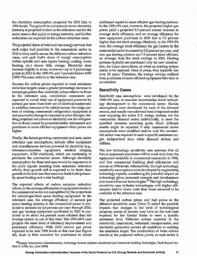
the electricity consumption projected for 2010 falls to1996 levels. The growth in commercial sector electricityintensity is projected to slow in the reference case for thesame reasons that apply to energy intensity, and furtherreductions are expected in the carbon reduction cases.
The projected share of total end-use energy services thateach major fuel provides to the commercial sector in2010 is fairly stable across the different carbon reductioncases, and each fuel's share of energy consumptionwithin specific end uses (space heating, cooling, waterheating, etc.) shows little change. Electricity doesincrease slightly in share, however—up to 2 percentagepoints in 2010 in the 1990-3% and 7-percent-below-1990(1990-7%) cases relative to the reference case.
Because the carbon prices required to meet emissionsreduction targets cause a greater percentage increase innatural gas prices than electricity prices relative to thosein the reference case, commercial consumers areexpected to curtail their use of equipment powered bynatural gas more than their use of electrical equipment.In addition, because of its critical nature, the usage pat-tern of existing commercial refrigeration equipment isnot assumed to change in response to price changes, lim-iting projected reductions in electricity use for refrigera-tion to those caused by potential earlier retirements andpurchases of more efficient equipment when prices arehigher.
Finally, the fastest-growing commercial end uses, underreference case assumptions, include office equipmentand miscellaneous devices powered by electricity (e.g.,telecommunications equipment, medical imagingequipment, ATM machines), which are continuing topenetrate the commercial sector. Although electricityconsumption for these end uses would be responsive tothe price signals resulting from emissions reductionefforts, their growth still is expected to be faster thangrowth in the end uses that consume fossil fuels (primar-ily space heating and water heating).
The expected effects of carbon emission reductionefforts on the average efficiencies of equipment stocks inthe commercial sector are exemplified by the projectionsfor natural-gas-fired space heating equipment. In thereference case, the average efficiency of natural gasspace heating systems in the commercial sector is pro-jected to increase by 0.6 percent per year through 2010,and gas heating equipment purchased in 2005 is pro-jected to be about 6.4 percent more efficient than theaverage system in use at that time. The 1990+24% caseprojects the same level of efficiency improvement andpurchased efficiency. With 2010 natural gas pricesexpected to be near 1996 levels in this case (see Figure40), there is little incentive for purchasers to invest
additional capital in more efficient gas heating systems.In the 1990+9% case, however, the projected higher gasprices yield a projected 0.7-percent annual increase inaverage stock efficiency and an average efficiency fornew equipment purchases in 2005 that is 7.2 percenthigher than the stock average. Similarly, in the 1990-3%case, the average stock efficiency for gas heaters in thecommercial sector increases by 0.8 percent per year, andnew gas heating systems are 7.5 percent more efficient,on average, than the stock average in 2005. Heatingsystems typically are purchased only for new construc-tion, for major renovations, or when an existing systemneeds to be replaced. Once in place, they typically lastover 20 years. Therefore, the energy savings realizedfrom purchases of more efficient equipment take time toaccumulate.
Sensitivity CasesSensitivity case assumptions were developed for the1990+9% case, to examine uncertainties about technol-ogy development in the commercial sector. Similarassumptions were developed for each of the demandsectors, and results were derived from integrated modelruns requiring the entire U.S. energy system, not thecommercial demand sector individually, to meet thespecified emission reduction goals. Much differentresults might be expected if only commercial sectorassumptions were modified and/or only the commer-cial sector was required to meet a specific emissions tar-get, independent from other demand sectors andutilities.
The low technology sensitivity case assumes that allfuture equipment purchases will be made only from theequipment available to commercial consumers in 1998,and that commercial building shell efficiencies willremain at 1998 levels. Alternatively, the high technologysensitivity assumptions were developed by engineeringtechnology experts, considering the potential impact ontechnology given increased research and developmentinto more advanced technologies.40 The high technologysensitivity case includes technologies with higher effi-ciencies and/or lower costs than those assumed to beavailable in the reference case.
The projected carbon prices and fuel prices in thedifferent sensitivity cases (Table 7) reflect the possibleimpacts that changes in the level of technologicalprogress, across all sectors, may have on the fuel costsrequired for the United States to meet a specificemissions level. Different actions expected in theresidential, commercial, industrial, transportation, andelectricity generation sectors all contribute to meetingthe emissions target. The combination of these actionsresults in the projected carbon prices, as each sector is
^Energy Information Administration, Technology Forecast Updates—Residential and Commercial Building Technologies, Draft Report (Ar-thur D. Little, Inc., June 1998).
Energy Information Administration / Impacts of the Kyoto Protocol on U.S. Energy Markets and Economic Activity 47

Photovoltaics and Fuel CellsIn every carbon reduction case considered in this report,neither photovoltaics nor fuel cells are projected to gainsignificant market penetration, because of their highcosts. With payback periods of more than 20 years, thesuccess of these technologies seems largely dependent onreducing production costs and increasing efficiency(which would result in further cost reductions for the con-sumer). Federal financial assistance would also play a rolein their success.
Currently, electricity from photovoltaics and fuel cells isapproximately 1.4 to 5.8 times the price to consumers ofelectricity from utility grids. Average prices in 1998 were79 mills per kilowatt for utility power, 112 mills for phos-phoric acid fuel cells (with no cogeneration), and 461 millsfor photovoltaic systems. To increase the market penetra-tion rates of the alternative technologies, their costswould have to be more competitive.
Photovoltaic and fuel cell technologies are examined hereon the basis of their potential for further market penetra-tion in 2010 for the 1990-3% case and in sensitivity casesassuming cost reductions (30 to 50 percent), performanceimprovements (50 percent for fuel cells, 70 percent forphotovoltaics), and Federal subsidies and credits. Pay-back periods are calculated for the regions where thesetechnologies are most likely to penetrate.
The effects of various private and government-assistedfinancing plans, such as rolling the cost of the alternativetechnology into a mortgage plan, tax credits, and depre-ciation, are summarized in the chart below. The first pairof bars shows the projected payback periods in 2010 forthe 1990-3% case with current technology performanceand costs. The other projections incorporate performanceimprovements of 50 percent for fuel cells and 70 percentfor photovoltaics, as well as the cumulative effects of vari-ous methods for reducing the payback periods. The sec-ond set of bars shows the effects of the assumedperformance improvement. The third includes a 30-percent production cost reduction, the fourth includes a
Projected Payback Periods for Photovoltaic andFuel Cell Purchases Under Different Assumptions,2010
Years
Performance201990-3% Improvement BFuel Cells - P V
15
10
Performance Improvementand 30% Cost Reduction
JPerformance Improvementand 50% Cost Reduction
M Performance Improvement,• 50% Cost Reduction, and• Mortgage IncorporationI Performance Improvement,
• • 50% Cost Reduction,^M I Mortgage Incorporation,^M I and Tax Credits
JSource: Energy Information Administration, Office of Integrated Analysis
and Forecasting.
50-percent cost reduction, the fifth includes the incorpo-ration of capital costs into a mortgage plan, and the sixthincludes a tax credit for photovoltaics and depreciationadjustments for businesses. It is important to note that thesubstantial cost reductions and improvements in effi-ciency (50 percent for fuel cells, 70 percent for photovol-taics) are merely arbitrary assumptions and are notcalculated projections for future costs and efficiencies.These assumptions are not included in the carbon reduc-tion cases or sensitivity cases presented in this report.
Under the most favorable assumptions shown in thegraph, payback periods could be reduced to less than 1year for fuel cells and 2 years for photovoltaics. Althoughpenetration levels are hard to predict from payback peri-ods, it can generally be assumed for the commercial andresidential sectors that paybacks within 3 to 4 yearswould be needed for significant penetration. In theNational Appliance Energy Conservation Act, the Federalefficiency payback standard for appliances is 3 years orless for investments to be non-burdensome to the con-sumer. Although some utilities may have payback peri-ods on their plants of 20 years, building consumers aremore likely to spend their money for efficient technolo-gies elsewhere if payback periods are over 4 years. Toachieve 3- to 4-year paybacks, both the current perform-ance and the costs of these alternatives would have to beimproved by the levels shown here; however, the likeli-hood of such substantial improvements in the next twodecades is small.
Production costs for photovoltaic modules have fallenfrom $100 per watt to $4 per watt over the past three dec-ades, an 11-percent annual decline, but since 1990 theyhave declined by an annual average of only 3.9 percent.3
To meet the cost reduction assumptions in these scenar-ios, the production costs for photovoltaic cells and mod-ules would have to decline at an average annual rate of 5.6percent through 2010.
The energy production efficiency of photovoltaic mod-ules has also improved, to approximately 12 percenttoday from 9 percent in 198O.b Reaching the goal of 70 per-cent improvement in performance, as assumed for thissensitivity analysis, would require an efficiency level of20 percent in 2010. Since 1980, the rate of improvement inperformance for photovoltaics has been less than 2 per-cent annually, whereas a 4.3-percent annual rate wouldbe needed to achieve a 70-percent improvement by 2010,and that improvement would also have to be accompa-nied by cost improvements to achieve a 3- to 4-year pay-back period. Fuel cells have been on the market for only ashort time, and historical information is not available.Neither technology appears to be on course to accomplishsuch a goal during the period of this analysis, however,and thus extensive market penetration is not probable foreither photovoltaics or fuel cells.
aEnergy Information Administration, Solar Collector Manu-facturing Activity 1991, DOE/EIA-0174(91), p. 18; and P. May-cock, "Photovoltaic Energy Conversion: PV Technology, Cost,Products, Markets, and Systems—Forecast 2010," ASES Con-ference (Albuquerque, NM, June 1998).
Paul Maycock, PV Energy, personal communication,August 1998.

Table 7. Projected Carbon Prices and Average FuelPrices for the Commercial Sector in \Technology Sensitivity Cases, 2010 [
Average !Carbon Price Fuel Price
(1996 Dollars per (1996 Dollars per >Analysis Case Metric Ton) Million Btu)
Reference — 11.51 |
1990+9% 163 17.99 J
11990+9% •Low Technology 243 21.66 j
1990+9% !I High Technology 121 15.75 II Source: Office of Integrated Analysis and Forecasting, National Energy Mod-eling System runs KYBASE.D080398A, FREE2E09.D080798A, FD09ABViD080398B, and HITECH09.D080698A. ',
expected to reduce demand in a way suitable to thatparticular sector.
Among the technology cases the highest carbon prices,and thus the highest fuel prices, in 2010 are projected inthe 1990+9% low technology sensitivity case. Due to thelack of technological progress in all sectors, higher fuelprices are required to achieve the demand reductionsneeded to reach the emissions target. The projected priceof fuel to the commercial sector is 20 percent higher inthe low technology case than in the 1990+9% case,resulting in 7 percent less commercial energy use.Commercial expenditures for fuel are also expected tobe highest under these conditions (Figure 43). Feweroptions for increased efficiency limit the potential forenergy savings in the low technology case. The averageefficiency of the equipment stock in this case continuesto improve as normal turnover takes place and olderequipment is replaced, but the most energy-efficientequipment available for purchase in 2010 or 2020 is whatis available today (Table 8).
Figure 43. Projected Fuel Expenditures in theCommercial Sector in Low and HighTechnology Cases, 1996-2020
2 0 0 -
1 5 0 -
1 0 0 -
50-
Billion 1996 Dollars
1990+9%Low Technology
Reference1990+9%
High Technology
0-r—1995 2000 2005 2010 2015 2020;
Source: Office of Integrated Analysis and Forecasting, National Energy!Modeling System runs KYBASE.D080398A, FREEZE09.D080798A, FD09ABV;
In the 1990+9% high technology sensitivity case, ad-vanced technologies are expected to penetrate themarket in all sectors over time as normal stock turnoverresults in the replacement of older, less efficientequipment. Projected technological advances through-out the energy market result in a carbon price in 2010that is 25 percent lower than that projected in the1990+9% case (see Table 7). In turn, the expected com-mercial fuel price in 2010 is 12 percent lower than in the1990+9% case, resulting in 4 percent more energy con-sumption. Even though more advanced technologies areavailable in the high technology case, with less priceincentive, commercial consumers are not as likely topurchase more costly equipment. For technologies suchas commercial natural gas water heaters, where high
Table 8. Projected Highest Available and Average Efficiencies for Newly Purchased Equipment in theCommercial Sector, 2015
Technology 19981990+9%
Low Technology
2.70
3.522.000.91
1.13
1.73
1.030.82
1990+9%
2.93
3.812.500.91
1.13
1.62
1.000.82
1990+9%High Technology
3.22
4.402.800.91
1.11
1.59
0.98
0.84
Highest Available Efficiency8
Air-Source Heat Pump
Natural Gas Chillers and Air Conditioners.
Heat Pump Water HeaterNatural Gas Water Heater
Average Purchased Efficiency3
Electric Space Heating
Natural Gas Space Cooling
Electric Water Heating
Natural Gas Water Heating
2.70
3.52
2.00
0.91
1.10
1.32
0.95
0.79aThe efficiencies shown (Btu of output divided by Btu of input) generally are seasonal efficiencies or include some measure of losses incurred
during normal use.I Source: Office of Integrated Analysis and Forecasting, National Energy Modeling System runs FREEZE09.D080798A, FD09ABV.D080398B, and HITECH09.;P080698A.
Energy Information Administration / Impacts of the Kyoto Protocol on U.S. Energy Markets and Economic Activity 49

technology assumptions specify lower costs in 2015 forthe most efficient equipment, as compared with the ref-erence case technology assumptions, more consumersare expected to adopt the efficient technology (see Table8). The projected reduction in energy demand in othersectors causes commercial fuel prices to decline in thelater years of the forecast, lowering commercial ex-penditures for fuel (Figure 43).
Industrial Demand
BackgroundThe industrial sector includes agriculture, mining, con-struction, and manufacturing activities. The sector con-sumes energy as an input to processes that produce thegoods that are familiar to consumers, such as cars andcomputers. The industrial sector also produces a widerange of basic materials, such as cement and steel, thatare used to produce goods for final consumption.Energy is an especially important input to the produc-tion processes of industries that produce basic materials.Typically, the industries that are energy-intensive arealso capital-intensive. Industries within the sector com-pete among themselves and with foreign producers forsales to consumers. Consequently, variations in inputprices can have significant competitive impacts. Themost significant determinant of industrial energy con-sumption is demand for final output.
Although energy is an important factor of production, itis not large in terms of annual manufacturing expendi-tures. In 1995, for example, purchased energy expendi-tures were 2.3 percent of annual manufacturingoutlays.41 Technology usually plays a minor role in thepattern of energy consumption, because technologytends to be used to produce new and improved finalproducts rather than to reduce energy consumption;however, when new investments are undertaken tointroduce improved production technology, steps toincrease energy efficiency also are undertaken. Overall,energy prices and technological breakthroughs tend tohave a rather small impact on industrial energy con-sumption.
The influence of energy prices on industrial energy con-sumption is modeled in terms of the efficiency of use ofexisting capital, the efficiency of new capital additions,and the mix of fuels used. This analysis uses "technologybundles" to characterize technological change in theenergy-intensive industries. This approach is dictatedby the number and complexity of processes used in theindustrial sector and the absence of systematic cost andperformance data for the components. These bundlesare defined for each production process step (e.g., cokeovens) for five of the industries and for end use (e.g.,refrigeration) in two of the industries. The process-stepindustries in the NEMS model are pulp and paper, glass,cement, steel, and aluminum.43 The industries for whichtechnology bundles are defined by end use are food andbulk chemicals.
The rate at which the average industrial energy intensitydeclines is determined primarily by the rate and timingof additions to manufacturing capacity. The rate andtiming of additions are functions of retirement rates andindustry growth rates. Typical retirement rates rangefrom 1 percent to 3 percent annually. The current modelalso allows retirement rates and the energy intensity ofnew additions to vary as a function of price. Price elastic-ity of demand, which indicates the responsiveness ofenergy consumption to changes in energy prices, is notan explicit assumption in the model; however, the typi-cal 20-year price elasticity ranges between -0.2 and -0.3,which indicates that a 1-percent price increase wouldreduce demand by 0.2 to 0.3 percent. Because the refer-ence case approximates a constant price regime, the ref-erence case results do not differ greatly from a situationin which all prices are held constant.
In 1996, the industrial sector's consumption of 34.6quadrillion Btu accounted for more than one-third of allU.S. energy consumption. The associated emissions of476 million metric tons of carbon accounted for one-third of all U.S. carbon emissions. In 1996, althoughindustrial energy prices were more than 50 percentlower than in 1980 (Figure 44), delivered energy con-sumption was only 13 percent higher than in 1980.Industrial output increased by more than 30 percentover that period. As a result, energy intensity (thousandBtu consumed per dollar of output) fell by 20 percent.
4 1 Calculated form U.S. Department of Commerce, 1995 Annual Survey of Manufactures, pp. 1-7 and 1-36.^For a variety of views, see Boyd et al., "Separating the Changing Composition of U.S. Manufacturing Production from Energy Effi-
ciency Improvements: A Divisia Index Approach," The Energy Journal, Vol. 8, No. 2 (1987); Doblin, "Declining Energy Intensity in the U.S.Manufacturing Sector," The Energy Journal, Vol. 9, No. 2 (1988); Howarth, "Energy Use in U.S. Manufacturing: The Impacts of the EnergyShocks on Sectoral Output, Industry Structure, and Energy Intensity," The Journal of Energy and Development, Vol. 14, No. 2 (1991); Jacard,Nyober, and Fogwill, "How Big is the Electricity Conservation Potential in Industry?" The Energy Journal, Vol. 14, No. 2 (1993); Steinmeyer,"Energy Use in Manufacturing," in Hollander, ed., The Energy-Environmental Connection (Island Press, 1992), Chapter 10; and U.S. Depart-ment of Energy, Comprehensive National Energy Strategy (Washington, DC, April 1998), pp. 13-14.
^The refining industry is modeled separately in the Petroleum Market Module of NEMS.

Figure 44. Index of Industrial Sector Energy Prices,2000-2020
Index, 2000=1.0 Industrial Delivered Energy Prices,History
3 .0 -
2.5-
2.0-
1.5-
. Index, 1970=1.0
1970 1975 1980 1985 1990
1,0-f—2000
'"-:---~ 1990-3%
1990+9%
1990+24%
Reference
2005 2010 2015 2020
Sources: History: Energy Information Administration, State Energy Price andExpenditure Report 1993, DOE/EIA-0376(93) (Washington, DC, December1995). Projections: Office of Integrated Analysis and Forecasting, NationalEnergy Modeling System runs KYBASE.DQ80398A, FD24ABV.D080398B;FD09ABV.D080398B, and FD03BLW.D080398B.
Most of the drop in energy intensity in the U.S.industrial sector occurred between 1980 and 1985, whenprices for both energy and capital inputs were rising andthe ability of U.S. manufacturers to compete inter-nationally was deteriorating. The recessions of 1980 and1981-1982 forced many less efficient plants to close,many permanently. Particularly hard hit were theprimary metals industries and motor vehicle manufac-turing. Output of the U.S. steel industry has neverrecovered to the levels of the late 1970s. Manufacturingprofits did not return to the levels attained in 1981 until1988.44 Energy prices certainly played a role in shapingthese changes in the industrial sector, but general eco-nomic conditions, recession, record high interest rates,and reduced ability of key industries to compete in inter-national markets were more important determinants ofchange.'45
In the reference case, industrial energy prices are pro-jected to increase very slightly or fall through 2010. Forexample, the price of natural gas is projected to increaseby 0.5 percent, and the price of electricity is projected tofall by 16 percent. From 1996 to 2010, industrial output isprojected to grow by 39 percent and energy consump-tion by only 16 percent. Industrial intensity falls by 17percent during the same period, approximating theintensity decline between 1980 and 1996. The factors thatare expected to produce the rapid decline in industrialenergy intensity despite moderate changes in energy
prices include a relative shift from, energy-intensive toless energy-intensive industries; replacement of existingequipment with less energy-intensive equipment asexisting capacity is retired; adoption of improved andless energy-intensive technologies; and the pressures ofinternational competition.
Carbon Reduction CasesIn the carbon reduction cases, the combined effect ofreduced demand for U.S. industrial output and higherenergy prices produces lower energy consumption thanin the reference case. Compared with the reference casein 2010, industrial output is $69 billion (1 percent) lowerin the 1990+24% case, $157 billion (3 percent) lower inthe 1990+9% case, and $308 billion (6 percent) lower inthe 1990-3% case (see Table 29 in Chapter 6).
Compared with the reference case, average energyprices in the industrial sector in 2010 are projected to be22 percent higher in the 1990+24% case, 55 percenthigher in the 1990+9% case, and 95 percent higher in the1990-3% case. In comparison, the industrial sector'saverage energy price increased by almost 189 percentfrom 1970 to 1980. Prices of all fuels are projected to behigher in the carbon reduction cases, with coal prices 135percent higher than the reference case in 2010 in the1990+24% case and natural gas prices 33 percent higher.The projected price increase for coal is attributable solelyto the projected carbon price, whereas the carbon priceand higher demand contribute about equally to theincrease for natural gas. In the 1990+9% case, natural gasand coal prices are projected to be 93 percent and 328percent higher, respectively, than in the reference case,and in the 1990-3% case they are 162 percent and 589 per-cent higher.
Lower projections of industrial output and higherprojected energy prices reduce the projections for deliv-ered energy consumption in the industrial sector by0.7 quadrillion Btu (2 percent) in the 1990+24% case, by1.3 quadrillion Btu (4 percent) in the 1990+9% case, andby 2.3 quadrillion Btu (7 percent) in the 1990-3% case in2010 relative to the reference case (Figure 45). In the1970-1980 period, industrial consumption was un-changed even though prices increased by 189 percent.Year-to-year industrial energy consumption began tofall in 1980, and the decline accelerated when generaleconomic conditions began to deteriorate during the1980 and 1981-1982 recessions. Energy consumptionreached its minimum in 1983, even though prices hadbegun to decline. These events reinforce the concept thatwhile energy prices do play a role in industrial energy
^Council of the Economic Advisers, Economic Report of the President (Washington, DC, February 1995), p. 381.45For example, see Boyd and Karlson, "Impact of Energy Prices on Technology Choice in the U.S. Steel Industry," The Energy Journal, Vol.
14, No. 2 (1993). More general discussion can be found in Berndt and Wood, "Energy Price Shocks and Productivity Growth: A Survey," inGordon et al., eds., Energy: Markets and Regulation (Cambridge, MA: MTT Press, 1987); and Berndt, "Energy Use, Technical Progress and Pro-ductivity Growth: A Survey of Economic Issues," Journal of Productivity Analysis, Vol. 2 (1990).
Energy Information Administration / Impacts of the Kyoto Protocol on U.S. Energy Markets and Economic Activity 51

Figure 45. Index of Delivered Energy Consumptionin the Industrial Sector, 1970-2020
Index, 1996=1.0
—Reference
—1990+24%—1990+14%
—1990+9%
—1990
— 1990-3%
—1990-7%
1.3-
1.2-
1.1-
1.0-
0.9-
0.8-
0.7-History Projections
1970 1980 1990 2000 2010 2020i
Sources: History: Energy Information Administration, State Energy DataReport 1995, DOE/EIA-0214(96) (Washington, DC, December 1997).;Projections: Office of Integrated Analysis and Forecasting, National EnergyModeling System runs KYBASE.D080398A, FD24ABV.D080398B, FD1998JD08D398B, FD09ABV.D080398B, FD1990.D080398B, FD03BLW.D080398B;and FD07BLW.D080398B. !
consumption, general and industry-specific economicconditions also play an important role.
Coal consumption is projected to drop sharply in thecarbon reduction cases, given its extreme pricedisadvantage. In the 1990+24% case, coal consumptionin 2010 is lower by 422 trillion Btu (16 percent) than inthe reference case; in the 1990+9% case it is 737 trillionBtu (28 percent) lower; and in the 1990-3% case it isabout 1 quadrillion Btu (36 percent) lower. The projectedreductions in coal consumption are predominantly dueto projected reductions in boiler fuel use.
The industrial sector consumes coal mainly as a boilerfuel and for production of coke in the iron and steelindustry. For example, 75 percent of manufacturing con-sumption of steam coal was used in boilers in 1994.46
Coal-fired boilers have substantially higher capital coststhan do gas-fired boilers, because of their materials han-dling requirements. For large steam loads, however,coal's price advantage over natural gas offsets its capitalcost disadvantage. But in the carbon reduction cases,coal suffers from both a capital cost and a fuel cost disad-vantage. As a result, a substantial amount of boiler fueluse switches from coal to natural gas and petroleumproducts.
The projected reduction in total steam coal consumptionin the industrial sector in 2010 (including for uses otherthan boiler fuel) in the 1990-3% case relative to the refer-ence case is more than 50 percent. Still, the reduction isless severe than that projected for the electric utility
sector. Electricity generators, in addition to switching tonatural gas, also have the available options of nuclearpower and renewable energy sources.
Consumption of metallurgical coal, which is used toproduce coke for iron and steel production, also isreduced sharply in the carbon reduction cases. Thereduction has several causes: substitution of natural gasin production processes, replacement of domestic cokeproduction with coke imports, replacement of somecoke-based steelmaking capacity with electricity-basedcapacity, and reduced production of domestic steel.
In the carbon reduction cases, natural gas consumptionis subject to two countervailing effects. The effect of gen-erally higher energy prices, and consequent lower levelsof industrial activity, is to reduce natural gas consump-tion. On the other hand, natural gas prices do notincrease by as much as the prices of competing fuels. Asnoted above, this results in relatively greater use of natu-ral gas as a boiler fuel. The carbon reduction cases alsoinduce additional cogeneration using natural gas, whichincreases natural gas consumption and reduces require-ments for other boiler fuels.
In the 1990+24% and 1990+9% cases, natural gas con-sumption is projected to increase slightly, because theimpact of increased boiler fuel use outweighs the reduc-tion caused by lower industrial output. In the 1990-3%case, natural gas consumption is unchanged from thereference case in 2010. Here, the drop in industrial out-put and the substitution for other boiler fuels have off-setting effects.
In the reference case, industrial carbon emissions areprojected to be 83 million metric tons higher in 2010 thanthey were in 1996 (Figure 46). Emissions attributable toincreased electricity consumption account for more thanhalf the increase. In contrast, electricity-based emissionsaccount for more than 70 percent of the emissionsreductions in the carbon cases. For example, in the1990+9% case, electricity-based carbon emissions in2010 are 79 million metric tons lower than in thereference case. A reduction of 19 million metric tons incarbon emissions from the combustion of fossil fuelsbrings industrial sector emissions to approximatelytheir 1990 level. Carbon emissions in the 1990-3% casefall to 418 million metric tons, 58 million tons below the1996 level and 35 million tons below the 1990 level.Again, electricity-based emissions account for three-fourths of the reduction from projected levels in thereference case.
Part of the reduction in electricity-based carbonemissions for the industrial sector is due to lowerelectricity consumption in the carbon reduction cases
^Energy Information Administration, Manufacturing Consumption of Energy 1994, DOE/EIA-0512(94) (Washington, DC, December1997), p. 168.

:igure 46. Industrial Sector Carbon Emissions,1990,1996, and 2010
7 0 0 -
6 0 0 -i1500-
Million Metric Tons
• Electric • :
Projections for 2010
Note: Electricity emissions are from the fossil fuels used to generate^ie electricity used in this sector.
Sources: History: Energy Information Administration, Emissions of
Greenhouse Gases in the United States 1996, DOE/EIA-0573(96) (Washington'JDC, October 1997). Projections: Office of Integrated Analysis and Forecasting,National Energy Modeling System runs KYBASE.D080398A, FD24ABV.D080398B, FD1998.D080398B, FD09ABV.D080398B, FD1990.D080398B,FD03BLW.D080398B, and FD07BLW.D080398B.
(Figure 47). A larger part of the reduction results fromsharply lower carbon intensity of electricity production.In the reference case, approximately 16.5 million metrictons of carbon are emitted in the production of 1quadrillion Btu of delivered electrical energy, ascompared with only 12.6 million metric tons in the1990+9% case and only 10.2 million metric tons in the1990-3% case (38 percent less than in the reference case).
Industrial energy intensity fell by 17 percent between1980 and 1996. In 1996, approximately 7,100 Btu ofenergy was required to produce a dollar's worth ofindustrial output. In the reference case energy intensitycontinues to fall, and in 2010 it is projected that only5,900 Btu will be required for each dollar of industrialoutput. The impact of the carbon reduction cases onindustrial energy intensity results from opposingeffects. The effect of higher energy prices is to reduceenergy intensity, whereas reduced or falling outputgrowth limits the amount of new, less energy-intensivecapital equipment that will be added to the existingstock, thereby retarding the rate of decline in energyintensity. Additional structural shifts in the compositionof industrial output further reduce energy intensity.(Fuel switching contributes to reduced carbon but doesnot affect energy intensity.)
The projected rate of decline in industrial energyintensity is smaller in the more stringent carbonreduction cases (Figure 48). Some process steps in theenergy-intensive industries approach the minimumlevel of energy intensity assumed to be practicallyachievable. In addition, in the more stringent carbonreduction cases, industrial output is more severely
Figure 47. Industrial Sector Energy Consumption| by Fuel, 1970,1980,1996, and 2010
Quadrillion Btu
• ~ e / : ; . - •NaturalGas •SteamCoal •Electricity14 - •Losses
History12-
Projections for 2010
1970 1980 1996 Reference 1990 1990 1990+24% +9% -3%
Sources: History: Energy Information Administration, State Energy Data'Peport 1995, DOE/EIA-0214(96) (Washington, DC, December 1997),Projections: Office of Integrated Analysis and Forecasting, National EnergyModeling System runs KYBASE.D080398A, FD24ABV.D080398B, FD09ABV.'fro80398B, and FD03BLW.D080398B,
Figure 48. Projected Energy Intensity in theIndustrial Sector, 1995-2020
Index, 1990=1.01.0-
0.9 - —Reference
—1990+24%
—1990+14%
— 1990+9%
0 . 8 - - 1 9 9 0
—1990-7%
Industrial Delivered Energy Intensity,History
Index, 1990=1.0
0.7'1995 2000 2005 2010 2015 2020Sources: History: Consumption: Energy Information Administration, State]
Energy Data Report 1995, DOE/EIA-0214(96) (Washington, DC, Decemberri 997). Output: Constructed by Standard & Poor's DRI from U.S. Department of^Commerce, "Benchmark Input-Output Accounts for the U.S. Economy, 1992:Make, Use, and Supplementary Tables," Survey of Current Business, November,{1997, and predecessor benchmark tables. Projections: Office of IntegratedAnalysis and Forecasting, National Energy Modeling System runs KYBASE^D080398A, FD24ABV.D080398B, FD1998.D080398B, FD09ABV.D080398BFD1990.D080398B, FD03BLW.D080398B, and FD07BLW.D080398B. '
reduced, resulting in smaller incentives for the additionof new, less energy-intensive capital equipment. Thechanges in energy intensity for the industrial subsectors(Figure 49) indicate that slower growth in output canlead to less pronounced declines in energy intensity inthe more stringent carbon reduction cases.
The change in aggregate industrial energy intensity canbe decomposed into two effects. One is the change inenergy intensity that results from a change in thecomposition of industrial output. For example, if the
Energy Information Administration / Impacts of the Kyoto Protocol on U.S. Energy Markets and Economic Activity 53
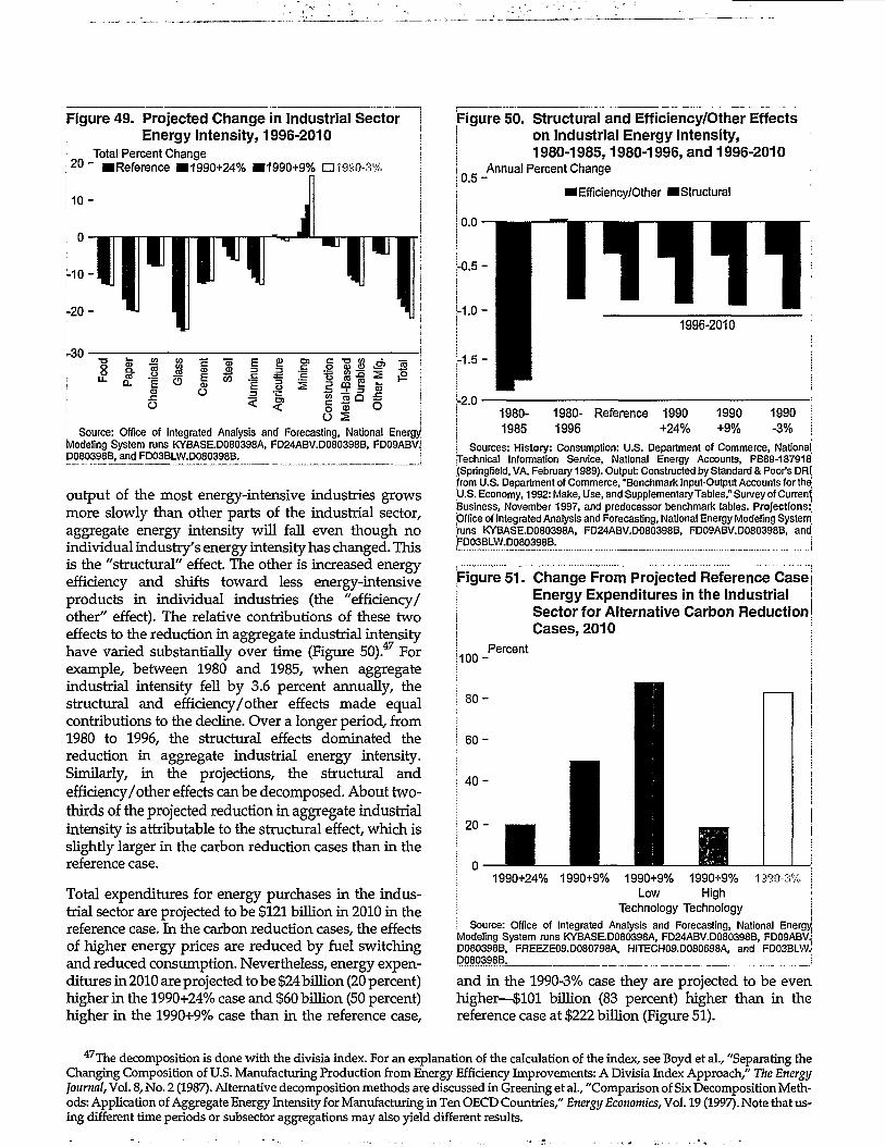
Figure 49. Projected Change in industrial Sectorj Energy Intensity, 1996-2010i Total Percent Change2 0 " •Reference •1990+24% •1990+9% •1990-3%
1 0 -
-20-
J%
r30
a. «
6CDO
•33 E 2 S>fl> 3 3 .=CO -f 3 | j
< i?
o "S S £> 1
§o
Source: Office of Integrated Analysis and Forecasting, National EnergyModeling System runs KYBASE.D080398A, FD24ABV.D080398B, FD09ABViD080398B, and FD03BLW.D080398B.
output of the most energy-intensive industries growsmore slowly than other parts of the industrial sector,aggregate energy intensity will fall even though noindividual industry's energy intensity has changed. Thisis the "structural" effect. The other is increased energyefficiency and shifts toward less energy-intensiveproducts in individual industries (the "efficiency/other" effect). The relative contributions of these twoeffects to the reduction in aggregate industrial intensityhave varied substantially over time (Figure 50).47 Forexample, between 1980 and 1985, when aggregateindustrial intensity fell by 3.6 percent annually, thestructural and efficiency/other effects made equalcontributions to the decline. Over a longer period, from1980 to 1996, the structural effects dominated thereduction in aggregate industrial energy intensity.Similarly, in tike projections, the structural andefficiency/other effects can be decomposed. About two-thirds of the projected reduction in aggregate industrialintensity is attributable to the structural effect, which isslightly larger in the carbon reduction cases than in thereference case.
Total expenditures for energy purchases in the indus-trial sector are projected to be $121 billion in 2010 in thereference case. In the carbon reduction cases, the effectsof higher energy prices are reduced by fuel switchingand reduced consumption. Nevertheless, energy expen-ditures in 2010 are projected to be $24 billion (20 percent)higher in the 1990+24% case and $60 billion (50 percent)higher in the 1990+9% case than in the reference case,
Figure 50. Structural and Efficiency/Other Effectsj on Industrial Energy Intensity,
1980-1985,1980-1996, and 1996-2010Annual Percent Change
Structural
1980-1985
1980- Reference 19901996 +24%
1990+9%
1990-3%
i Sources: History: Consumption: U.S. Department of Commerce, NationalTechnical Information Service, National Energy Accounts, PB89-187918|(Springfield, VA, February 1989). Output: Constructed by Standard & Poor's DR|from U.S. Department of Commerce, "Benchmark Input-Output Accounts for thdU.S. Economy, 1992: Make, Use, and Supplementary Tables," Survey of CurrentBusiness, November 1997, and predecessor benchmark tables. Projections^Office of Integrated Analysis and Forecasting, National Energy Modeling Systemjuns KYBASE.D080398A, FD24ABV.D080398B, FD09ABV.D080398B, andFD03BLW.D080398B.
Figure 51. Change From Projected Reference CaseEnergy Expenditures in the IndustrialSector for Alternative Carbon ReductionCases, 2010
1 0 0 -
8 0 -
6 0 -
Percent
1990+24% 1990+9% 1990+9% 1990+9% 1990-3%Low High
Technology TechnologySource: Office of Integrated Analysis and Forecasting, National Energy!
Modeling System runs KYBASE.D080398A, FD24ABV.D080398B, FD09ABVJD080398B, FREEZE09.D080798A, HITECH09.D080698A, and FD03BLWJb080398B. !
and in the 1990-3% case they are projected to be evenhigher—$101 billion (83 percent) higher than in thereference case at $222 billion (Figure 51).
47The decomposition is done with the divisia index. For an explanation of the calculation of the index, see Boyd et al., "Separating theChanging Composition of U.S. Manufacturing Production from Energy Efficiency Improvements: A Divisia Index Approach," The EnergyJournal, Vol. 8, No. 2 (1987). Alternative decomposition methods are discussed in Greening et al., "Comparison of Six Decomposition Meth-ods: Application of Aggregate Energy Intensity for Manufacturing in Ten OECD Countries," Energy Economics, Vol. 19 (1997). Note that us-ing different time periods or subsector aggregations may also yield different results.

Sensitivity Cases
The projections of industrial sector energy expendituresin the carbon reduction cases are based on the referencecase assumptions about technology improvements andlikely industrial response. Expenditures would be muchhigher if technology improvements occurred at a slowerrate than in the reference case. On the other hand, a moreoptimistic technology outlook would reduce energyexpenditures.
To span the technology alternatives, low and high tech-nology sensitivity cases, based on the 1990+9% carbonreduction case, were analyzed. The low technology case
assumes that no additional technology changes (asreflected in energy intensity) will occur after 1998. Nor-mal turnover of capital, however, would result in somedecline in energy intensity as old equipment is replacedwith currently available equipment with lower energyintensity. The high technology case assumes an aggres-sive private and Federal commitment to energy-relatedresearch and development, which results in successfulcommercialization of energy-saving technologies.48
As noted earlier, the analysis uses technology bundlesto characterize technological change in the energy-intensive industries. This approach is illustratedin Table 9. For example, the energy intensity of the
[Table 9. Projected Energy Intensities for Industrial Process Steps and End UsesIndustry/Process Step or End Use | 1990+9% Low Technology 1990+9% | 1990+9% High Technology
FoodDirect Fuel
Hot Water/Steam
RefrigerationOther Electric
Pulp and Paper
Paper Making
BleachingWaste Fiber PulpingMechanical PulpingSemi-Chemical
Kraft, Sulfite, misc
Wood PreparationBulk Chemicals
ElectrolyticOther ElectricDirect FuelSteam/Hot WaterFeedstocks
GlassPost-FormingForming
Melting/RefiningBatch Preparation
CementFinish GrindingDry ProcessWet Process
Steel
Cold Rolling
Hot RollingIngot Casting/Primary RollingContinuous CastingBlast Furnace/Basic Oxygen Furnace.
Electric Arc Furnace
Coke Oven
Primary Aluminum
1.001.00
1.00
1.00
1.00
1.00
1.00
1.001.001.001.001.001.001.001.001.001.001.001.001.001.001.001.001.001.001.001.001.001.001.001.001.001.001.001.001.001.00
0.89
0.88
0.89
0.90
0.90
0.78
0.77
0.860.940.920.860.780.950.950.910.900.880.890.990.730.910.890.630.960.850.820.830.930.810.560.651.001.081.101.001.000.87
0.790.790.790.790.790.640.620.780.870.960.910.610.920.850.830.830.830.830.870.590.940.880.410.990.770.720.660.970.500.330.371.001.060.500.620.980.71
Notes: The energy intensity for the low technology case is defined as 1.0. The 1990+9% case and high technology case energy intensities arendexed against the energy intensity for the low technology case. The intensities are not additive within an industry.
Source: The high technology sensitivity case is based in part on an analysis prepared by Arthur D. Little, Inc., Aggressive Technology Strategy for the NEMS Model(1998). :
48The high technology sensitivity case is based in part on an analysis prepared by Arthur D. Little, Inc., Aggressive Technology Strategy forthe NEMS Model (1998).
Energy Information Administration / Impacts of the Kyoto Protocol on U.S. Energy Markets and Economic Activity 55

Cogeneration SystemsIn every carbon reduction case considered in this report,neither photovoltaics nor fuel cells are projected to gainsignificant market penetration, because of their highcosts. With payback periods of more than 20 years, thesuccess of these technologies seems largely dependent onreducing production costs and increasing efficiency(which would result in further cost reductions for the con-sumer). Federal financial assistance would also play a rolein their success.
A key issue facing power producers and their customersis whether the types of cogeneration systems currentlyused in the United States will be extended to include dis-trict energy systems and advanced turbine systems(ATS). Cogeneration systems, also called combined heatand power systems, simultaneously produce heat in theform of hot air or steam and power in the form of electric-ity by a single thermodynamic process, usually steamboilers or gas turbines, reducing the energy losses thatoccur when process steam and electricity are producedindependently. Thus, cogeneration systems could play asignificant role in reducing U.S. greenhouse gas emis-sions.
In 1996, electric utilities used more than 21 quadrillionBtu of energy from the combustion of coal, natural gas,and oil to produce the equivalent of only 7 quadrillion Btuof electricity available at the plant gate, representing aconversion loss of 67 percent.8 Consequently, unusedwaste heat at utility plants accounted for 346 million met-ric tons or nearly 24 percent of U.S. carbon emissions in1996. Additional losses on the order of 7 percent areincurred during transmission and distribution of electric-ity to customers.13 Because cogeneration systems captureand use a significant portion of the waste heat energy,they are nearly twice as efficient as conventional powerplants in extracting usable energy. About 6 percent oftotal U.S. generating capacity includes some type ofcogeneration system, in such diverse industries as manu-facturing, mining, and refining.0
Some energy analysts believe that there is even greaterpotential to increase the penetration of cogeneration sys-tems and reduce carbon emissions by wide-scale con-struction of district energy systems. District energysystems distribute chilled water, steam, or hot water tobuildings to provide air conditioning, space heating,domestic hot water, and industrial process energy. About5,800 district energy systems are installed in the UnitedStates, serving more than 8 percent of commercial floor-space—primarily military bases, universities, hospitals,downtown areas, and other group buildings.
The greatest growth potential for district energy systemsis in the area of utility-financed cooling systems for down-town areas where there is a large amount of commercialfloorspace located in a relatively small area; however.
significant hurdles must be overcome if the potential is tobe realized. Siting one or more power and steam genera-tors in an area already dense with buildings could proveto be a challenge, as could the installation, maintenance,and repair of lines to carry steam and hot or chilled watersupplies in cities with under-street congestion of existinggas, water, sewage, and electricity lines. Also, construc-tion costs for district energy systems are about one-thirdhigher than those for conventional generating technolo-gies.
Although it is possible that fuel cost savings over the lifeof a district energy plant could offset its higher initial con-struction cost, electricity producers might be reluctant toinvest significant capital during a period of regulatoryreform. Even after the current restructuring process inU.S. electricity markets is completed, the risk of nonre-covery of capital for capital-intensive technologies in acompetitive environment will make finding investors insuch projects a challenge. Moreover, the development of adistrict energy system involves the coordinated effort oflocal and State governments, investors, and the commu-nity as a whole, together with the subsequent legal, finan-cial, and environmental issues that arise with theinclusion of many and diverse stakeholders.
Another technology that some energy analysts believecould significantly reduce greenhouse gas emissions isthe next-generation, very-high-efficiency ATS. These tur-bines are expected to operate, at minimum, 5 to 10 percentmore efficiently than steam boilers and to cost less than$350 Der kilowatthour when used as a simple-cycle tur-bine. Their small size (5 megawatts) and short construc-tion and delivery schedule (18 months) result in relativelysmaller capital outlays and faster capital recovery, whichare expected to give them an economic advantage overlarge central-station turbines.
Commercialization of ATS turbines is not expected until2001, and penetration is expected to occur first wherethere is a need to satisfy internal power and steamrequirements at industrial and large commercial estab-lishments. But large-scale penetration of the ATS technol-ogy as envisioned by its advocates depends on thedevelopment of a significant niche market for thiscogeneration system—a market characterized as having asmall, but not constant, demand for steam. ATS inelectric-only mode may not be competitive with other pri-mary power technologies, and a constant demand forsteam could be satisfied more economically by conven-tional gas and combined-cycle steam boilers. Conse-quently, the competitiveness of ATS with othergenerating technologies depends on locating marketswith an optimal demand for steam during part of the dayand maximum demand for electricity for the remainder ofthe day, even during off-peak periods. Few, if any, powermarkets would meet such stringent criteria.
^Energy Information Administration, Annual Energy Review 1996, DOE/EIA-0384(96) (Washington, DC, July 1997).Interlaboratory Working Group on Energy-Efficient and Low-Carbon Technologies, "Scenarios of U.S. Carbon Reductions,"
LBNL-40533, ORNL/CON-444 (September 1997)."Energy Information Administration, Annual Energy Outlook 1998, DOE/EIA-0383(98) (Washington, DC, December 1997).See web site www.energy.rochester.edu/us/climate/abstract.htm, "District Energy in U.S. Climate Change Strategy."
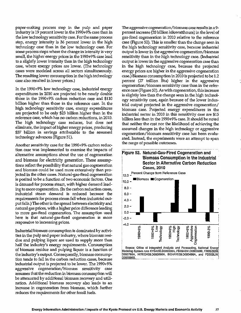
paper-making process step in the pulp and paperindustry is 19 percent lower in the 1990+9% case than inthe low technology sensitivity case. For the same processstep, energy intensity is 36 percent lower in the hightechnology case than in the low technology case. Forsome process steps where the change in intensity is verysmall, the higher energy prices in the 1990+9% case leadto a slightly lower intensity than in the high technologycase, where energy prices are lower. (The technologycases were modeled across all sectors simultaneously.The resulting lower consumption in the high technologycase also resulted in lower prices.)
In the 1990+9% low technology case, industrial energyexpenditures in 2010 are projected to be nearly doublethose in the 1990+9% carbon reduction case and $110billion higher than those in the reference case. In thehigh technology sensitivity case, energy expendituresare projected to be only $23 billion higher than in thereference case, which has no carbon reductions, in 2010.The high technology case reduces, but does noteliminate, the impact of higher energy prices, producing$37 billion in savings attributable to the assumedtechnology advances (Figure 51).
Another sensitivity case for the 1990+9% carbon reduc-tion case was implemented to examine the impacts ofalternative assumptions about the use of cogenerationand biomass for electricity generation. These assump-tions reflect the possibility that natural gas cogenerationand biomass could be used more extensively than pro-jected in the other cases. Natural-gas-fired cogenerationis posited to be a function of two economic factors. Oneis demand for process steam, with higher demand lead-ing to more cogeneration. (In the carbon reduction cases,industrial steam demand is reduced because therequirements for process steam fall when industrial out-put falls.) The other is the spread between electricity andnatural gas prices, with a higher price difference leadingto more gas-fired cogeneration. The assumption usedhere is that natural-gas-fired cogeneration is moreresponsive to increasing prices.
Industrial biomass consumption is dominated by activi-ties in the pulp and paper industry, where biomass resi-due and pulping liquor are used to supply more thanhalf the industry's energy requirements. Consumptionof biomass residue and pulping liquor is a function ofthe industry's output. Consequently, biomass consump-tion tends to fall in the carbon reduction cases, becauseindustrial output is projected to be lower. The 1990+9%aggressive cogeneration/biomass sensitivity caseassumes that the reduction in biomass consumption willbe attenuated by additional biomass recovery and utili-zation. Additional biomass recovery also leads to anincrease in cogeneration from biomass, which furtherreduces the requirements for other fossil fuels.
The aggressive cogeneration/biomass case results in a 9-percent increase (20 billion kilowatthours) in the level ofgas-fired cogeneration in 2010 relative to the referencecase (Figure 52). This is smaller than the change seen inthe high technology sensitivity case, because industrialoutput is lower in the aggressive cogeneration/biomasssensitivity than in the high technology case. (Industrialoutput is lower in the aggressive cogeneration case thanin the high technology case, because the projectedenergy prices are higher in the aggressive cogenerationcase.) Biomass consumption in 2010 is projected to be 1.2percent (27 trillion Btu) higher in the aggressivecogeneration/biomass sensitivity case than in the refer-ence case (Figure 52). As with cogeneration, this increaseis slightly less than the change seen in the high technol-ogy sensitivity case, again because of the lower indus-trial output projected in the aggressive cogeneration/biomass case. Projected energy expenditures in theindustrial sector in 2010 in this sensitivity case are $15billion less than in the 1990+9% case. It should be notedthat neither the cost nor the likelihood of achieving theassumed changes in the high technology or aggressivecogeneration/biomass sensitivity case has been evalu-ated. Instead, the experiments were an attempt to spanthe range of possible outcomes.
Figure 52. Natural-Gas-Fired Cogeneration andBiomass Consumption in the IndustrialSector in Alternative Carbon ReductionCases, 2010
112.0 -
10.0-
Percent Change from Reference Case
I Biomass •Cogeneration
2.0-
0.0
-2.0-
-4.0-
+oCD 5 -5
o o o oc <n c en
-5|2
.> ,gto ^a> |s S
en
enCO
8Source: Office of Integrated Analysis and Forecasting, National Energy
Modeling System runs KYBASE.D080398A, FD09ABV.D080398B, FREEZE09JD080798A, HITECH09.D080698A, BEHAVE09.D080498A, and FD03BLW.D080398B.
Energy Information Administration / Impacts of the Kyoto Protocol on U.S. Energy Markets and Economic Activity 57

Industrial CompositionBecause non-Annex I countries are not required to reduceemissions under the Kyoto Protocol, their energy pricesare likely to be lower than those in the Annex I countries,including the United States. As a result, more energy-intensive industries could migrate from areas with highenergy costs, and those that remain could lose markets tolower-cost foreign competition. Energy-intensive indus-tries also may face reduced demand as consumers shifttheir consumption patterns to less energy-intensivegoods and services. There are several counter argumentsto this hypothesis: the relatively small share of energyexpenditures in annual manufacturing expendituresmakes the impact of differential energy prices relativelyunimportant; energy prices are not important determi-nants of international trade or capital flows, whichimplies that U.S. energy-intensive industries are notlikely to be seriously affected by an energy price disad-vantage; and a large number of business opportunitiesrelated to climate change mitigation will become avail-able both domestically and in non-Annex I countries.Needless to say, there are widely divergent points of viewabout the likelihood of significant industrial migrationand the extent of adverse impacts on U.S. industry.3 Ananalysis of the change in industrial composition, whichwould require an analysis of all the relative costs of manu-facturing inputs, of which energy costs are only one,monetary issues, and international trade issues, is beyondthe scope of this report.
One published study has attempted to evaluate the poten-tial effects of differential changes in international energyprices on the U.S. industrial sector. The study was con-ducted by Argonne National Laboratory in a workshopformat (see Argonne National Laboratory, The Impact ofHigh Energy Price Cases on Energy-Intensive Sectors: Per-spectives from Industry Workshops (July 1997)). Industry-specific discussion papers circulated to workshop partici-pants contained analyses that examined impacts for eachindividual industry, assuming no price changes for other
industries or markets. The industries affected and the per-centage reductions in projected industrial output in thereference case were as follows: bulk chemicals, 28.5; alu-minum, 13.7; pulp and paper, 10.2; steel, 30.5; and cement,38.2.
A second study was conducted at EIA's request by Char-les River Associates (CRA),b using a more generalapproach. Explicit linkages to international trade were afundamental part of the modeling framework for thestudy, which was conducted under assumptions similarto those of the 1990+14% carbon reduction case in thisanalysis. The industries affected and the percentagereductions from reference case output projections were asfollows: total chemicals, 3.9; nonferrous metals, 1.5; pulpand paper plus printing, 0.7; steel, 1.4; and nonmetallicminerals, 1.4. The percentage output reductions from thecomparable NEMS case (1990+14%) are about double theCRA values: nonferrous metals, 4.4; pulp and paper plusprinting, 2.0; steel, 3.1; and nonmetallic minerals, 3.5. Theexception is total chemicals for which the NEMS resultsproject a slightly smaller reduction of 3.5 percent. Theprojections from NEMS, which estimates only domesticoutput reductions, and from CRA, which treated bothinternational capital flows and domestic output reduc-tions, are significantly lower than those from the ArgonneNational Laboratory study.
In view of the above results, it is difficult to distinguishthe effects of reduced output from those that could resultfrom industrial migration abroad in response to differ-ences in international energy prices. There are many ana-lytical complexities in the assessment of potential effectsof carbon reductions on industrial output. A completeanalysis of the issue would require consideration of allinput costs, including infrastructure and locationaladvantages, monetary issues, and trade issues. Signifi-cant additional research would be required to examinethe differential impacts of climate change policies on theUnited States and other countries.
aThe following authors provide a sample of the breadth of disagreement in this area: American Petroleum Institute, Impacts ofMarket-Based Greenhouse Gas Emission Reduction Policies on U.S. Manufacturing Competitiveness, January 1998; American AutomobileManufacturers Association, Economic Implications of the Adoption of Limits on Carbon Emissions from Industrialized Countries, November1997; Argonne National Laboratory, The Impact of High Energy Price Cases on Energy-Intensive Sectors: Perspectives from Industry Work-shops, July 1997; Matthewson, et al., The Economic Implications for Canada and the United States of International Climate Change Policies,1997 Canadian Energy Research Institute Environment-Energy Modeling Forum, October 1997; Repetto, et al., U.S. Competitiveness isNot at Risk in the Climate Negotiations, (World Resources Institute, October 1997); and WEFA, Inc., Global Warming: The High Cost of theKyoto Protocol, National and State Impacts, 1998.
Charles River Associates, Report to the Energy Information Administration (August 1998).

Transportation Demand
BackgroundIn terms of primary energy use in 1996, transportationsector carbon emissions, which almost equaled indus-trial carbon emission levels, were the second highestamong the end-use demand sectors. Nearly 33 percentof all carbon emissions and 78 percent of carbon emis-sions from petroleum consumption originate from thetransportation sector. In the reference case, carbon emis-sions from transportation are projected to grow at anaverage annual rate of 1.9 percent to 2010, comparedwith 1.4 percent for the commercial sector and 1.2 per-cent for both the residential and industrial sectors. Inaddition, transportation is the only sector with increas-ing carbon emissions projected for the period from 2010to 2020 in the carbon reduction cases. Therefore, if thereare no specific initiatives to reduce carbon emissions inthe transportation sector, especially beyond 2010,increasing pressure may have to be exerted in the othersectors in order to reach and then maintain 2010 carbonemissions targets beyond 2010.
Consumers select light-duty vehicles (cars, vans, pick-up trucks, and sport utility vehicles) based on a numberof attributes: size, horsepower, price, and cost of driving;weighting these attributes by their personal preferences.This analysis uses past experience to determine theweights that each of these attributes have in terms ofconsumer preferences for conventional vehicles. Tech-nologies are represented by component (e.g., frontwheel drive, electronic transmission type) with eachtechnology component defined by a date of introduc-tion, a cost, and a weight that indicates its impact on effi-ciency and horsepower. The vehicles are categorized bythe 12 size classes for cars and light trucks defined by theEnvironmental Protection Agency and includes 2 con-ventional engine technologies, and 14 alternative fuelvehicle engine technologies. Technologies penetratebased on both their cost-effectiveness and by consumerpreference based on past experience with similar tech-nologies in the automotive industry. Consumers areassumed to consider only current energy prices whenevaluating technologies. However, it is assumed that theautomobile industry requires 3 years for minor technol-ogy makeovers and 5 years for major redesigns, estimat-ing future fuel prices based on their rate of growth in thepast 3 to 5 years. Therefore, manufacturers considerwhether future fuel prices will enable their technologiesto be cost-effective from a consumer standpoint.
Penetration of alternative-fuel vehicles is based on fourconsumer criteria—vehicle price, cost of driving permile, vehicle range, and availability of refueling stations.Each of these attributes is weighted according to con-sumer surveys and expected changes over the forecastperiod as a result of technological improvements, larger
scales of production, the availability and cost of fuel-saving technologies, and the availability of alternative-fuel refueling stations as more alternative-fuel vehiclespenetrate the market. Production levels for alternative-fuel vehicles are constrained by the lead time to switchproduction to a particular technology and the availabil-ity of technologies in each size class.
Depending on per capita income, fuel prices, and fueleconomy, consumers may switch to either smaller sizeclasses or smaller vehicles with lower horsepowerrequirements within a size class. The trend in vehiclesales toward or away from light trucks (vans, sport util-ity vehicles, and pickups) is determined by fuel prices.Vehicle travel is determined by the cost of driving permile and per capita income. For flex-fuel or bi-fuelalternative-fuel vehicles, the percentage use of each fuelis based on the price differential between gasoline andthe alternative fuel.
Responding to changes in fuel prices, gasoline has a 2-year demand elasticity of -0.25 and a 20-year elasticity of-0.45. In the long term, consumers are expected to altertheir purchasing patterns and manufacturers to incorpo-rate more fuel-saving technologies. Because fuel use forfreight trucks and trains depends primarily on require-ments for freight movement as a result of economicactivity and the slow turnover of the stock, distillate fuelhas lower 2-year and 20-year price elasticities, at -0.09and -0.13, respectively. In addition to fuel prices, busi-ness and personal air travel also depend on grossdomestic product (GDP) and per capita income, respec-tively, and have very slow rates of stock turnover. Jetfuel has 2-year and 20-year elasticities of -0.12 and -0.15.
Energy intensity in the transportation sector is definedas energy use (in terms of gallons of gasoline) per vehicleper year. In the reference case, transportation energyintensity in 2010 is projected to be about 635 gallons ofgasoline per vehicle, or about 53 gallons per month(Figure 53). Energy intensity in the 1990+24% case islower than in the reference case but only by 12 gallons ofgasoline per car per month. In the 1990+9% case, theprojected energy intensity in 2010 is almost 53 gallonslower—equivalent to 1 month's use of gasoline. Inthe 1990-3% and 1990-7% cases, the correspondingreductions in gasoline consumption in 2010 areequivalent to nearly 1.5 and 2 months of gasoline use,respectively.
In the absence of fuel price changes, transportationenergy intensity will change in response to stockturnover, technology availability, and income effects(Table 10). Because 1998 prices are lower than thoseprojected for 2010 in the reference case, vehicle-milestraveled would be higher and fuel efficiency lower thanin the reference case if the 1998 price level continued.Constant 1998 fuel prices would slightly increase air
Energy Information Administration / Impacts of the Kyoto Protocol on U.S. Energy Markets and Economic Activity 59
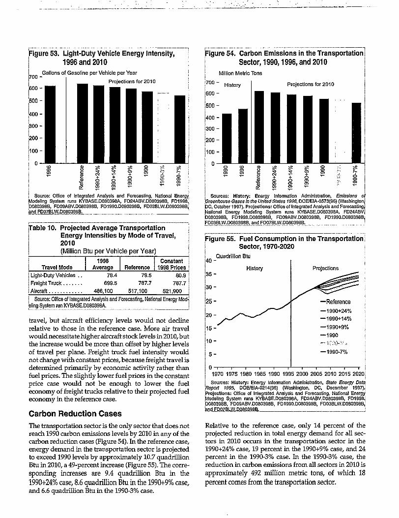
Figure 53. Light-Duty Vehicle Energy Intensity,1996 and 2010
Gallons of Gasoline per Vehicle per Year
Projections for 2010
Source: Office of Integrated Analysis and Forecasting, National EnergyModeling System runs KYBASE.D080398A, FD24ABV.D080398B, FD1998JD080398B, FD09ABV.D080398B, FD1990.D080398B, FD03BLW.D080398B,!
and FD07BLW.D080398B.
Table 10. Projected Average TransportationEnergy Intensities by Mode of Travel,2010(Million Btu per Vehicle per Year)
Travel Mode1998
Average ReferenceConstant
1998 PricesLight-Duty Vehicles . .
Freight Truck
Aircraft
78.4
699.5
486,100
79.5
787.7
517,100
80.9
787.7
521,900
Source: Office of Integrated Analysis and Forecasting, National Energy Modfeling System run KYBASE.D080398A.
travel, but aircraft efficiency levels would not declinerelative to those in the reference case. More air travelwould necessitate higher aircraft stock levels in 2010, butthe increase would be more than offset by higher levelsof travel per plane. Freight truck fuel intensity wouldnot change with constant prices, because freight travel isdetermined primarily by economic activity rather thanfuel prices. The slightly lower fuel prices in the constantprice case would not be enough to lower the fueleconomy of freight trucks relative to their projected fueleconomy in the reference case.
Carbon Reduction CasesThe transportation sector is the only sector that does notreach 1990 carbon emissions levels by 2010 in any of thecarbon reduction cases (Figure 54). In the reference case,energy demand in the transportation sector is projectedto exceed 1990 levels by approximately 10.7 quadrillionBtu in 2010, a 49-percent increase (Figure 55). The corre-sponding increases are 9.4 quadrillion Btu in the1990+24% case, 8.6 quadrillion Btu in the 1990+9% case,and 6.6 quadrillion Btu in the 1990-3% case.
Figure 54. Carbon Emissions in the Transportation!Sector, 1990,1996, and 2010
Million Metric Tons
i 7 0 0 -
£ CM
OCDCD
•^OCDCD
CD
OCDCD
OCDCD
CD
Sources: History: Energy Information Administration, Emissions ofGreenhouse Gases in the United States 1996, DOE/EIA-0573(96) (Washington,t)C, October 1997). Projections: Office of Integrated Analysis and Forecasting,Rational Energy Modeling System runs KYBASE.D080398A, FD24ABV,D080398B, FD1998.D080398B, FD09ABV.D080398B, FD1990.D080398B<FD03BLW.D080398B, and FD07BLW.D080398B. 1
Figure 55. Fuel Consumption in the Transportation ji Sector, 1970-2020 i
! 4 0 -
3 5 -
130 -
iJ25-J20 -!
I10-
i 5 -
Quadrillion Btu
History Projections
—Reference—1990+24%
—1990+14%
-1990+9%
—1990
— 1990-7%
1970 1975 1980 1985 1990 1995 2000 2005 2010 2015 2020!j I
Sources: History: Energy Information Administration, State Energy DataPeport 1995, DOE/EIA-0214(96) (Washington, DC, December 1997);Projections: Office of Integrated Analysis and Forecasting, National Energy!Modeling System runs KYBASE.D080398A, FD24ABV.D080398B, FD1998JD080398B, FD09ABV.D080398B, FD1990.D080398B, FD03BLW.D080398B<!
k J
Relative to the reference case, only 14 percent of theprojected reduction in total energy demand for all sec-tors in 2010 occurs in the transportation sector in the1990+24% case, 19 percent in the 1990+9% case, and 24percent in the 1990-3% case. In the 1990-3% case, thereduction in carbon emissions from all sectors in 2010 isapproximately 492 million metric tons, of which 18percent comes from the transportation sector.
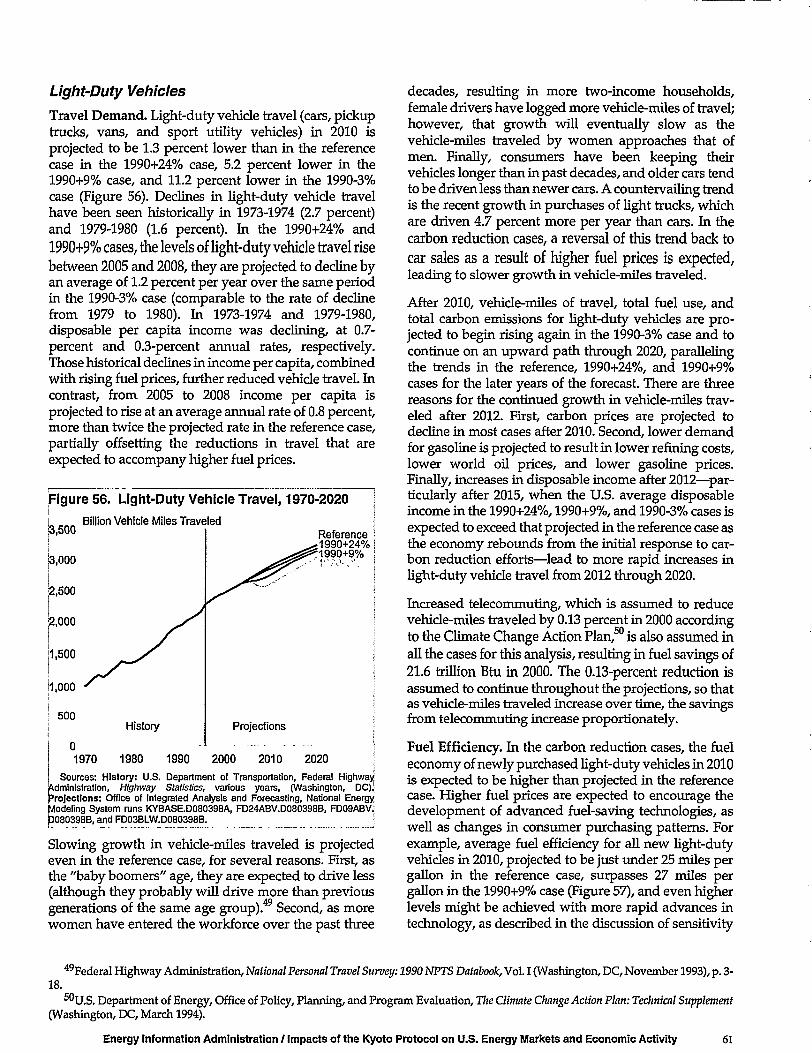
Light-Duty Vehicles
Travel Demand. Light-duty vehicle travel (cars, pickuptrucks, vans, and sport utility vehicles) in 2010 isprojected to be 1.3 percent lower than in the referencecase in the 1990+24% case, 5.2 percent lower in the1990+9% case, and 11.2 percent lower in the 1990-3%case (Figure 56). Declines in light-duty vehicle travelhave been seen historically in 1973-1974 (2.7 percent)and 1979-1980 (1.6 percent). In the 1990+24% and1990+9% cases, the levels of light-duty vehicle travel risebetween 2005 and 2008, they are projected to decline byan average of 1.2 percent per year over the same periodin the 1990-3% case (comparable to the rate of declinefrom 1979 to 1980). In 1973-1974 and 1979-1980,disposable per capita income was declining, at 0.7-percent and 0.3-percent annual rates, respectively.Those historical declines in income per capita, combinedwith rising fuel prices, further reduced vehicle travel. Incontrast, from 2005 to 2008 income per capita isprojected to rise at an average annual rate of 0.8 percent,more than twice the projected rate in the reference case,partially offsetting the reductions in travel that areexpected to accompany higher fuel prices.
Figure 56. Light-Duty Vehicle Travel, 1970-2020
Billion Vehicle Miles Traveledb,500
J3.000
k,500
11,000
500History
Reference1990+24%19909%
Projections
1970 1980 1990 2000 2010 2020Sources: History: U.S. Department of Transportation, Federal Highway)
Administration, Highway Statistics, various years, (Washington, DC),projections: Office of Integrated Analysis and Forecasting, National EnergyModeling System runs KYBASE.D080398A, FD24ABV.D080398B, FD09ABV.£080398B, and FD03BLW.D080398B.
Slowing growth in vehicle-miles traveled is projectedeven in the reference case, for several reasons. First, asthe "baby boomers" age, they are expected to drive less(although they probably will drive more than previousgenerations of the same age group). Second, as morewomen have entered the workforce over the past three
decades, resulting in more two-income households,female drivers have logged more vehicle-miles of travel;however, that growth will eventually slow as thevehicle-miles traveled by women approaches that ofmen. Finally, consumers have been keeping theirvehicles longer than in past decades, and older cars tendto be driven less than newer cars. A countervailing trendis the recent growth in purchases of light trucks, whichare driven 4.7 percent more per year than cars. In thecarbon reduction cases, a reversal of this trend back tocar sales as a result of higher fuel prices is expected,leading to slower growth in vehicle-miles traveled.
After 2010, vehicle-miles of travel, total fuel use, andtotal carbon emissions for light-duty vehicles are pro-jected to begin rising again in the 1990-3% case and tocontinue on an upward path through 2020, parallelingthe trends in the reference, 1990+24%, and 1990+9%cases for the later years of the forecast. There are threereasons for the continued growth in vehicle-miles trav-eled after 2012. First, carbon prices are projected todecline in most cases after 2010. Second, lower demandfor gasoline is projected to result in lower refining costs,lower world oil prices, and lower gasoline prices.Finally, increases in disposable income after 2012—par-ticularly after 2015, when the U.S. average disposableincome in the 1990+24%, 1990+9%, and 1990-3% cases isexpected to exceed that projected in the reference case asthe economy rebounds from the initial response to car-bon reduction efforts—lead to more rapid increases inlight-duty vehicle travel from 2012 through 2020.
Increased telecommuting, which is assumed to reducevehicle-miles traveled by 0.13 percent in 2000 accordingto the Climate Change Action Plan,50 is also assumed inall the cases for this analysis, resulting in fuel savings of21.6 trillion Btu in 2000. The 0.13-percent reduction isassumed to continue throughout the projections, so thatas vehicle-miles traveled increase over time, the savingsfrom telecommuting increase proportionately.
Fuel Efficiency. In the carbon reduction cases, the fueleconomy of newly purchased light-duty vehicles in 2010is expected to be higher than projected in the referencecase. Higher fuel prices are expected to encourage thedevelopment of advanced fuel-saving technologies, aswell as changes in consumer purchasing patterns. Forexample, average fuel efficiency for all new light-dutyvehicles in 2010, projected to be just under 25 miles pergallon in the reference case, surpasses 27 miles pergallon in the 1990+9% case (Figure 57), and even higherlevels might be achieved with more rapid advances intechnology, as described in the discussion of sensitivity
49Federal Highway Administration, National Personal Travel Survey: 1990 NPTS Databook, Vol. I (Washington, DC, November 1993), p. 3-18.
^U.S. Department of Energy, Office of Policy, Planning, and Program Evaluation, The Climate Change Action Plan: Technical Supplement(Washington, DC, March 1994).
Energy Information Administration / Impacts of the Kyoto Protocol on U.S. Energy Markets and Economic Activity 61
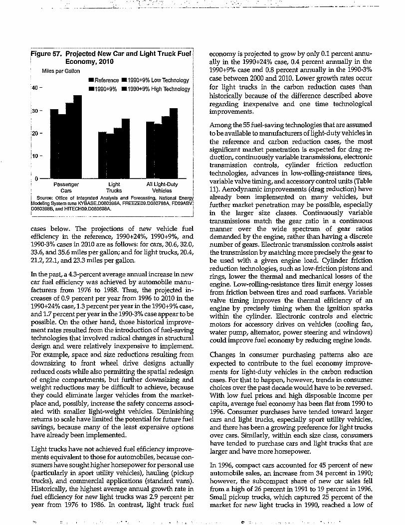
Figure 57. Projected New Car and Light Truck FuelEconomy, 2010
Miles per Gallon {
•Reference •1990+9% Low Technology j
40 - • 1990+9% • 1990+9% High Technology
3 0 -
2 0 -
1 0 -
PassengerCars
LightTrucks
All Light-DutyVehicles
Source: Office of Integrated Analysis and Forecasting, National EnergyModeling System runs KYBASE.D080398A, FREEZE09.D080798A, FD09ABV]D080398B, and HITECH09.D080698A. !
cases below. The projections of new vehicle fuelefficiency in the reference, 1990+24%, 1990+9%, and1990-3% cases in 2010 are as follows: for cars, 30.6,32.0,33.6, and 35.6 miles per gallon; and for light trucks, 20.4,21.2,22.1, and 23.3 miles per gallon.
In the past, a 4.3-percent average annual increase in newcar fuel efficiency was achieved by automobile manu-facturers from 1976 to 1988. Thus, the projected in-creases of 0.9 percent per year from 1996 to 2010 in the1990+24% case, 1.3 percent per year in the 1990+9% case,and 1.7 percent per year in the 1990-3% case appear to bepossible. On the other hand, those historical improve-ment rates resulted from the introduction of fuel-savingtechnologies that involved radical changes in structuraldesign and were relatively inexpensive to implement.For example, space and size reductions resulting fromdownsizing to front wheel drive designs actuallyreduced costs while also permitting the spatial redesignof engine compartments, but further downsizing andweight reductions may be difficult to achieve, becausethey could eliminate larger vehicles from the market-place and, possibly, increase the safety concerns associ-ated with smaller light-weight vehicles. Diminishingreturns to scale have limited the potential for future fuelsavings, because many of the least expensive optionshave already been implemented.
Light trucks have not achieved fuel efficiency improve-ments equivalent to those for automobiles, because con-sumers have sought higher horsepower for personal use(particularly in sport utility vehicles), hauling (pickuptrucks), and commercial applications (standard vans).Historically, the highest average annual growth rate infuel efficiency for new light trucks was 2.9 percent peryear from 1976 to 1986. In contrast, light truck fuel
economy is projected to grow by only 0.1 percent annu-ally in the 1990+24% case, 0.4 percent annually in the1990+9% case and 0.8 percent annually in the 1990-3%case between 2000 and 2010. Lower growth rates occurfor light trucks in the carbon reduction cases thanhistorically because of the difference described aboveregarding inexpensive and one time technologicalimprovements.
Among the 55 fuel-saving technologies that are assumedto be available to manufacturers of light-duty vehicles inthe reference and carbon reduction cases, the mostsignificant market penetration is expected for drag re-duction, continuously variable transmissions, electronictransmission controls, cylinder friction reductiontechnologies, advances in low-rolling-resistance tires,variable valve timing, and accessory control units (Table11). Aerodynamic improvements (drag reduction) havealready been implemented on many vehicles, butfurther market penetration may be possible, especiallyin the larger size classes. Continuously variabletransmissions match the gear ratio in a continuousmanner over the wide spectrum of gear ratiosdemanded by the engine, rather than having a discretenumber of gears. Electronic transmission controls assistthe transmission by matching more precisely the gear tobe used with a given engine load. Cylinder frictionreduction technologies, such as low-friction pistons andrings, lower the thermal and mechanical losses of theengine. Low-rolling-resistance tires limit energy lossesfrom friction between tires and road surfaces. Variablevalve timing improves the thermal efficiency of anengine by precisely timing when the ignition sparkswithin the cylinder. Electronic controls and electricmotors for accessory drives on vehicles (cooling fan,water pump, alternator, power steering and windows)could improve fuel economy by reducing engine loads.
Changes in consumer purchasing patterns also areexpected to contribute to the fuel economy improve-ments for light-duty vehicles in the carbon reductioncases. For that to happen, however, trends in consumerchoices over the past decade would have to be reversed.With low fuel prices and high disposable income percapita, average fuel economy has been flat from 1990 to1996. Consumer purchases have tended toward largercars and light trucks, especially sport utility vehicles,and there has been a growing preference for light trucksover cars. Similarly, within each size class, consumershave tended to purchase cars and light trucks that arelarger and have more horsepower.
In 1996, compact cars accounted for 45 percent of newautomobile sales, an increase from 34 percent in 1990;however, the subcompact share of new car sales fellfrom a high of 26 percent in 1991 to 19 percent in 1996.Small pickup trucks, which captured 25 percent of themarket for new light trucks in 1990, reached a low of
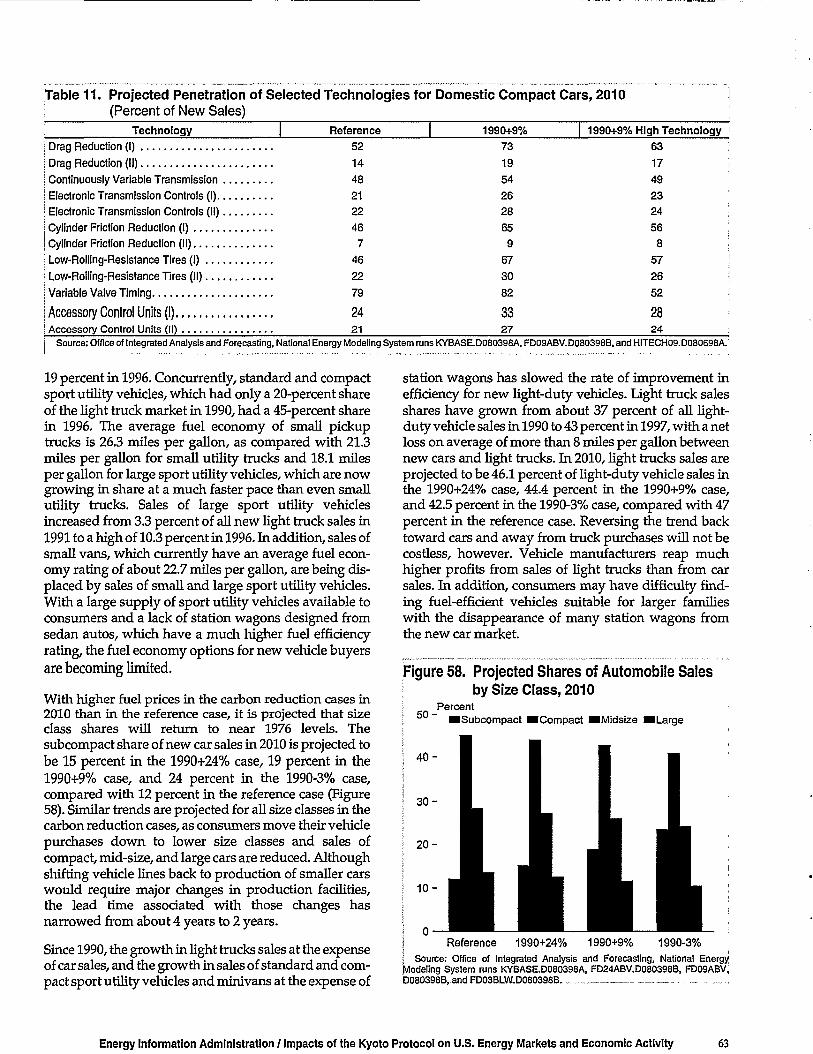
Table 11. Projected Penetration of Selected Technologies for Domestic Compact Cars, 2010| (Percent of New Sales)
Technology Reference I 1990+9% 1990+9% High Technology
I Drag Reduction (I) ,
I Drag Reduction (II)
I Continuously Variable Transmission ,
i Electronic Transmission Controls (I).,
i Electronic Transmission Controls (II),
I Cylinder Friction Reduction (I) ,
j Cylinder Friction Reduction (II)
| Low-Rolling-Resistance Tires (I)
| Low-Rolling-Resistance Tires (II)
Variable Vaive Timing ,
Accessory Control Units (I)Accessory Control Units (II)
52
14
48
21
22
46
7
46
22
79
2421
73
19
54
26
28
65
9
67
30
82
3327
63
17
49
23
24
56
8
57
26
52
2824
Source: Office of Integrated Analysis and Forecasting, National Energy Modeling System runs KYBASE.D080398A, FD09ABV.D080398B, and HITECH09.D080698A. |
19 percent in 1996. Concurrently, standard and compactsport utility vehicles, which had only a 20-percent shareof the light truck market in 1990, had a 45-percent sharein 1996. The average fuel economy of small pickuptrucks is 26.3 miles per gallon, as compared with 21.3miles per gallon for small utility trucks and 18.1 milesper gallon for large sport utility vehicles, which are nowgrowing in share at a much faster pace than even smallutility trucks. Sales of large sport utility vehiclesincreased from 3.3 percent of all new light truck sales in1991 to a high of 10.3 percent in 1996. In addition, sales ofsmall vans, which currently have an average fuel econ-omy rating of about 22.7 miles per gallon, are being dis-placed by sales of small and large sport utility vehicles.With a large supply of sport utility vehicles available toconsumers and a lack of station wagons designed fromsedan autos, which have a much higher fuel efficiencyrating, the fuel economy options for new vehicle buyersare becoming limited.
With higher fuel prices in the carbon reduction cases in2010 than in the reference case, it is projected that sizeclass shares will return to near 1976 levels. Thesubcompact share of new car sales in 2010 is projected tobe 15 percent in the 1990+24% case, 19 percent in the1990+9% case, and 24 percent in the 1990-3% case,compared with 12 percent in the reference case (Figure58). Similar trends are projected for all size classes in thecarbon reduction cases, as consumers move their vehiclepurchases down to lower size classes and sales ofcompact, mid-size, and large cars are reduced. Althoughshifting vehicle lines back to production of smaller carswould require major changes in production facilities,the lead time associated with those changes hasnarrowed from about 4 years to 2 years.
Since 1990, the growth in light trucks sales at the expenseof car sales, and the growth in sales of standard and com-pact sport utility vehicles and minivans at the expense of
station wagons has slowed the rate of improvement inefficiency for new light-duty vehicles. Light truck salesshares have grown from about 37 percent of all light-duty vehicle sales in 1990 to 43 percent in 1997, with a netloss on average of more than 8 miles per gallon betweennew cars and light trucks. In 2010, light trucks sales areprojected to be 46.1 percent of light-duty vehicle sales inthe 1990+24% case, 44.4 percent in the 1990+9% case,and 42.5 percent in the 1990-3% case, compared with 47percent in the reference case. Reversing the trend backtoward cars and away from truck purchases will not becostless, however. Vehicle manufacturers reap muchhigher profits from sales of light trucks than from carsales. In addition, consumers may have difficulty find-ing fuel-efficient vehicles suitable for larger familieswith the disappearance of many station wagons fromthe new car market.
Figure 58. Projected Shares of Automobile SalesI by Size Class, 2010
5 0 -
4 0 -
3 0 -
PercentISubcompact •Compact •Midsize •Large
20-
1 0 -
Reference 1990+24% 1990+9% 1990-3%Source: Office of Integrated Analysis and Forecasting, National Energy
Modeling System runs KYBASE.D080398A, FD24ABV.D080398B, FD09ABV,D080398B,.and ED03BLW.D080398B '.
Energy Information Administration / Impacts of the Kyoto Protocol on U.S. Energy Markets and Economic Activity 63
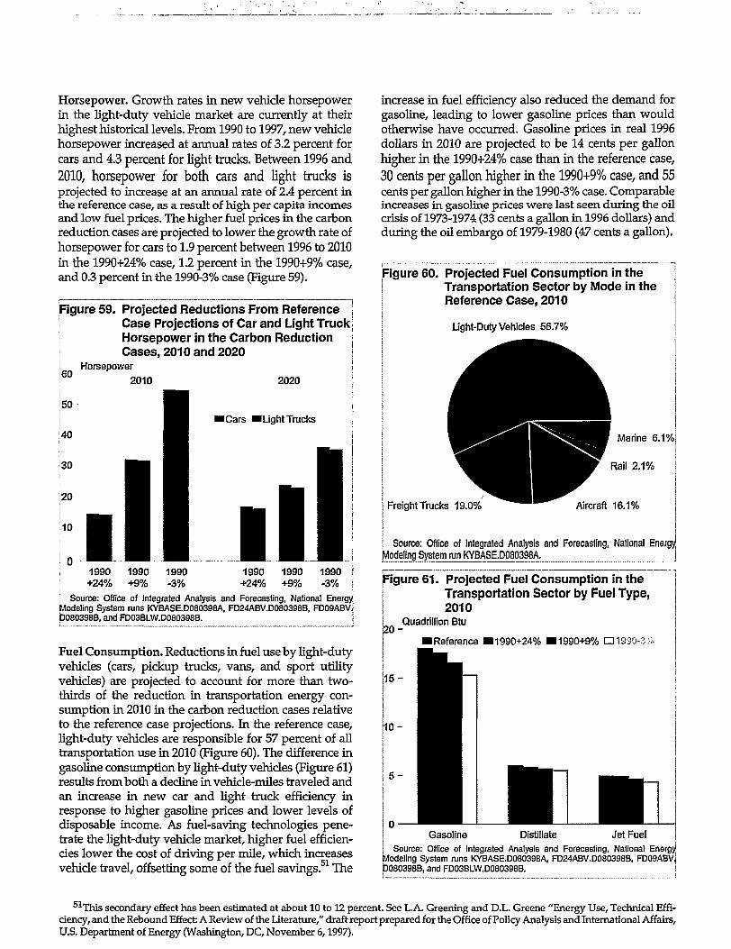
Horsepower. Growth rates in new vehicle horsepowerin the light-duty vehicle market are currently at theirhighest historical levels. From 1990 to 1997, new vehiclehorsepower increased at annual rates of 3.2 percent forcars and 4.3 percent for light trucks. Between 1996 and2010, horsepower for both cars and light trucks isprojected to increase at an annual rate of 2.4 percent inthe reference case, as a result of high per capita incomesand low fuel prices. The higher fuel prices in the carbonreduction cases are projected to lower the growth rate ofhorsepower for cars to 1.9 percent between 1996 to 2010in the 1990+24% case, 1.2 percent in the 1990+9% case,and 0.3 percent in the 1990-3% case (Figure 59).
Figure 59. Projected Reductions From Reference jCase Projections of Car and Light Truck!Horsepower in the Carbon Reduction jCases, 2010 and 2020 j
Horsepower j
2010 2020 I60
50
40
30
20
10
I Cars •Light Trucks
1990 1990+24% +9%
1990 1990+24% +9%
Source: Office of Integrated Analysis and Forecasting, National EnergyModeling System runs KYBASE.D080398A, FD24ABV.D080398B, FD09ABV.'D080398B, and FD03BLW.D080398B.
Fuel Consumption. Reductions in fuel use by light-dutyvehicles (cars, pickup trucks, vans, and sport utilityvehicles) are projected to account for more than two-thirds of the reduction in transportation energy con-sumption in 2010 in the carbon reduction cases relativeto the reference case projections. In the reference case,light-duty vehicles are responsible for 57 percent of alltransportation use in 2010 (Figure 60). The difference ingasoline consumption by light-duty vehicles (Figure 61)results from both a decline in vehicle-miles traveled andan increase in new car and light truck efficiency inresponse to higher gasoline prices and lower levels ofdisposable income. As fuel-saving technologies pene-trate the light-duty vehicle market, higher fuel efficien-cies lower the cost of driving per mile, which increasesvehicle travel, offsetting some of the fuel savings.51 The
increase in fuel efficiency also reduced the demand forgasoline, leading to lower gasoline prices than wouldotherwise have occurred. Gasoline prices in real 1996dollars in 2010 are projected to be 14 cents per gallonhigher in the 1990+24% case than in the reference case,30 cents per gallon higher in the 1990+9% case, and 55cents per gallon higher in the 1990-3% case. Comparableincreases in gasoline prices were last seen during the oilcrisis of 1973-1974 (33 cents a gallon in 1996 dollars) andduring the oil embargo of 1979-1980 (47 cents a gallon).
Figure 60. Projected Fuel Consumption in theTransportation Sector by Mode in theReference Case, 2010
Light-Duly Vehicles 56.7%
Freight Trucks 19.0%
Marine 6.1%
Rail 2.1%
Aircraft 1 6 . 1 %
Source: Office of Integrated Analysis and Forecasting, National EnergyModeling System run KYBASE.D080398A.
Figure 61. Projected Fuel Consumption in theTransportation Sector by Fuel Type,2010
2 0 -Quadrillion Btu
•Reference ^ 1 9 9 0 + 2 4 % ^ 1 9 9 0 + 9 % • 1990-3 «•
0Gasoline Distillate Jet Fuel
Source: Office of Integrated Analysis and Forecasting, National Energy1
Modeling System runs KYBASE.D080398A, FD24ABV.D080398B, FD09ABV,D080398B, and FD03BLW.D080398B.
51This secondary effect has been estimated at about 10 to 12 percent. See L.A. Greening and D.L. Greene "Energy Use, Technical Effi-ciency, and the Rebound Effect A Review of the Literature," draft report prepared for the Office of Policy Analysis and International Affairs,U.S. Department of Energy (Washington, DC, November 6,1997).

Air TravelPersonal, business, and international air travel areexpected to decline in response to higher jet fuel pricesand higher ticket prices in the carbon reduction cases, ascompared with the reference case, from 2005 through2015. The projected levels of air travel in 2010 are 1.4 per-cent lower in the 1990+24% case than in the referencecase, 7.4 percent lower in the 1990+9% case, and 16.0 per-cent lower in the 1990-3% case. Higher fuel prices in 2010are projected to increase ticket prices by 5 percent, 13percent, and 23 percent in the 1990+24% case, 1990+9%and 1990-3% cases, respectively, over the reference caseprices. Lower merchandise exports (0.9 percent lower inthe 1990+24% case, 2.5 percent in the 1990+9% case, and4.9 percent in the 1990-3% case than in the referencecase) have comparable effects on dedicated air freighttravel.
Between 2005 and 2008, air travel is projected to declineby 1.2 percent annually in the 1990-3% case as a result ofa 19-percent average annual increase in jet fuel prices. Incomparison, air travel declined by 2.2 percent from 1980to 1981, when jet fuel prices increase by 49 percent. Simi-lar to light-duty vehicles, differences in the responses tohigher fuel prices between history and the carbon reduc-tion cases can be explained by comparing growth ratesin income levels. Income during 2005 to 2008 is expectedto increase by 0.8 percent annually in the carbon reduc-tion cases, however from 1980 to 1981 income was risingeven faster at 2.3 percent per year, which mitigated thedecline in air travel.
In 2010, the projected use of jet fuel is lower by 1.4 per-cent in the 1990+24% case than in the reference case, by6.6 percent in the 1990+9% case, and by 14.2 percent inthe 1990-3% case (Figure 61). Jet fuel prices are projectedto be 15 cents per gallon higher than in the reference casein 2010 in the 1990+24% case, 34 cents per gallon higherin the 1990+9% case, and 63 cents per gallon higher inthe 1990-3% case.
Only relatively minor changes in the average fuel effi-ciency of new aircraft are expected to result from theimposition of carbon reduction targets. For example, inthe 1990+9% case, new aircraft fuel efficiency is pro-jected to improve at an annual rate of just 0.9 percentbetween 1996 and 2010, compared with the 0.7-percentrate projected in the reference case. As a result, the aver-age efficiencies projected for the entire U.S. stock of air-craft are nearly the same in the two cases (Figure 62).
Less air travel is expected in the carbon reduction casesthan in the reference case, leading to slower rates of air-craft stock turnover, which in turn limit the penetrationof new aircraft into the aircraft stock. Higher fuel pricesand lower air travel in the carbon reduction cases lowerthe demand for wide-body aircraft, which have higherefficiencies in terms of seat-miles per gallon than do
narrow-body aircraft. In addition, near-term aircrafttechnologies that can improve fuel efficiency are limited,and they are not expected to be cost-effective even in the1990-3% case. Among the six advanced aircraft tech-nologies available by 2010, only weight-reducing mate-rials and ultra-high-bypass engines, which are currentlyin use, are expected to penetrate the market (Table 12);and only the ultra-high-bypass engine technology isprojected to achieve significant penetration (more than90 percent) by 2010, and then only in the 1990-3% case orthe high technology sensitivity case described below.
figure 62. Projected New and Stock Aircraft FuelI Efficiency, 2010
•90 -i
Seat-Miles per Gallon
•Reference •1930*9% Lev Technology
•1990+9% •1990+9% High Technology
Stock Aircraft
! Source: Office of Integrated Analysis and Forecasting, National EnergyModeling System runs KYBASE.D080398A, FREEZE09.D080798A, FD09ABV.-D080398B, and HITECH09.D080698A.
Table 12. Projected Penetration for Selectedi Advanced Technologies for Aircraft,| 2010| (Percent of New Sales)
Technology Reference 1990+9%
1990+9%High ;
Technology
I Ultra-High-BypassI Engines
i Weight-Reducingi Materials
! Advanced
i AerodynamicsI Thermodynamics .
9
85
0
0
90
85
0
0
77
96
96
56
I Source: Office of Integrated Analysis and Forecasting, National Energy Mod-eling System runs KYBASE.D080398A, FD09ABV.D080398B, ancjHITECH09.D080698A. :
Freight Trucks, Rail, and ShippingThe projected demand for distillate fuel, used primarilyfor freight trucks and rail, is also lower in the carbonreduction cases than in the reference case in 2010—by 2percent in the 1990+24% case, by 4.9 percent in the1990+9% case, and by 8.3 percent in the 1990-3% case(see Figure 61). Distillate fuel prices are projected to be
Energy Information Administration / Impacts of the Kyoto Protocol on U.S. Energy Markets and Economic Activity 65

15 cents per gallon higher in the 1990+24% case, 37 centsper gallon higher in the 1990+9% case and 68 centshigher in the 1990-3% case. These increases are largerthan those projected for gasoline because of the highercarbon content of distillate fuel.
Higher fuel prices do not result in as much change intravel and efficiency for freight trucks and rail as they dofor light-duty vehicles. Because of the slow turnover inthe stock of freight trucks and rail and the high powerrequirements of the engines used to move freight, fuelsavings are limited. The main source of reductions indistillate fuel use is the response to overall lower eco-nomic activity and demand for goods by 2010 in the car-bon reduction cases, leading to lower freight travel forboth trucks and rail. Lower demand for goods in the1990+24%, 1990+9% and 1990-3% cases results in levelsof freight truck travel that are 1.3 percent, 2.4 percentand 4.9 percent lower, respectively, in 2010 than pro-jected in the reference case. Declines in coal consump-tion and production also lead to further cuts in rail travelas described below.
The potential for improvement in fuel economy forfreight trucks is also limited. In the reference case, thefuel efficiency of new freight trucks is projected toincrease by only 0.6 percent per year between 1996 and2010. Even with higher distillate fuel prices in the 1990-3% case, the efficiency for new freight trucks improves atan annual rate of only 0.8 percent. As a result of thelower demand for goods and slower turnover in thestock of freight trucks projected in the 1990+9% case
The number of advanced technologies available forfreight trucks is relatively small. Those with the greatestpotential are advanced aerodynamics, the turbo-compound diesel engine, and the LE-55 heat engine,with expected marginal fuel efficiency improvements ofapproximately 25, 10, and 17 percent, respectively(Table 13). In all the carbon reduction cases, theadvanced aerodynamics technology is projected toachieve the greatest efficiency improvements andhighest penetration rates for both medium- and heavy-duty trucks. The turbo-compound diesel engine and theLE-55 heat engine do not penetrate the market until after2010, except in the high technology sensitivity cases.
In percentage terms, the projections for rail and shipfreight travel in 2010 show the sharpest reductionsrelative to the reference case in the carbon reductioncases. Rail freight travel is 9 percent, 23 percent, and 32percent lower in 2010 in the 1990+24%, 1990+9%, and1990-3% cases than in the reference case. Since more than40 percent of rail travel is for coal transportation, thelower rail travel in the carbon reduction cases isprimarily due to the projected reductions in coalproduction of 20 percent, 52 percent, and 71 percent inthe 1990+24%, 1990+9%, and 1990-3% cases relative tothe reference case. Domestic freight travel by ship isprojected to be 3 percent, 6 percent, and 10 percent lowerin the three cases than in the reference case. Domesticshipping is not expected to be affected as adversely bythe decline in coal production as is rail traffic; however,with lower demand for goods and industrial production
relative to the reference case, there is almost no differ-ence in the projected average stock efficiencies for thetwo cases in 2010 (Figure 63).
Figure 63. Projected New and Stock Freight TruckFuel Efficiency, 2010
Miles per Gallon S10 I
•Reference •1990+9% Low Technology j
8 •1990+9% •1990+9% High Technology j
Table 13. Projected Penetration of SelectedTechnologies for Freight Trucks, 2010(Percent of I
Technology
Medium Trucks
Improved Tiresand LubricantsElectronicEngine Controls
AdvancedDrag Reduction
Turbo Compound Diesel.
LE-55 Heat Engine
^ ^ ^ ^ ^ ^ ^ ^ H ^ ^ ^ ^ ^ ^ ^ ^ | | Heavy Trucks
o ^ ^ —New Freight Trucks Stock Freight Trucks
Source: Office of Integrated Analysis and Forecasting, National EnergyModeling System runs KYBASE.D080398A, FREEZE09.D080798A, FD09ABVD080398B, and H1TECH09.D080698A.
Improved Tiresand Lubricants
ElectronicEngine Controls
AdvancedDrag Reduction
Turbo Compound Diesel.
1 LE-55 Heat Engine
view Sales)
Reference
0
0
23
0
0
0
0
100
1
0
1990+9%
0
0
34
2
0
3
4
100
1
0
1990+9%High
Technology
0
5
45
8
13
98 j
98 !
100
35
10 !j Source: Office of Integrated Analysis and Forecasting, National Energy Mod-eling System runs KYBASE.D080398A, FD09ABV.D080398BD080698A.
, and HITECH09,

in the carbon reduction cases, domestic shipping is alsoprojected to be lower.
Like freight truck and rail travel, shipping is affectedmore by the impacts of carbon prices on travel and ship-ping requirements than by the direct impacts of higherfuel costs. High-carbon residual fuel has the largest pro-jected price increases of all the transportation fuels, withincrements of 19 cents per gallon in the 1990+24% case,46 cents in the 1990+9% case, and 84 cents—almost 100percent—in the 1990-3% case relative to the prices pro-jected for 2010 in the reference case.
Approximately 15 to 17 percent of the drop in total fuelconsumption in 2010 in the carbon reduction cases isattributed to aircraft, 6 to 7 percent to freight trucks, 4 to6 percent to rail engines, and 1 percent to marineengines. The relative energy consumption shares for themajor transportation modes and fuels do not varysignificantly across the cases (Table 14).
Table 14. Projected Fuel Consumption Shares inthe Transportation Sector by Fuel andTravel Mode, 2010(Percent of Total) i
Projection ReferenceFuel
Gasoline 58
Distillate 19
Jet Fuel 16
Residual 4
Alternative Fuels
Travel Mode
Light-Duty Vehicles..
Freight Trucks
Aircraft
Rail
3
5717162
Marine 6
1990+24%
5819
16
4
3
56191626
1990+9%
57
20
16
4
3
56201626
1990-3%
56
21
16
5
3
55201627
Source: Office of Integrated Analysis and Forecasting, National Energy Mod-Bling System runs KYBASE.D080398A, FD24ABV.D080398B, FD09ABV.1
D080398B, and FD03BLW.D080398B.
Both freight rail and domestic shipping efficiencies areprojected to remain at reference case levels in the carbonreduction cases. Stock turnover will virtually cease,because rail ton-miles traveled are lower by 32 percent in2010 in the 1990-3% case than in the reference case, anddomestic shipping travel is 10 percent lower. Also, withthe loss in revenue associated with the projected lowerlevels of travel, efficiency improvements will be difficultto achieve.
Alternative-Fuel VehiclesAccording to consumer surveys, alternative-fuel vehiclesales are dependent on vehicle price, the cost of drivingper mile, vehicle range, fuel availability, and commercial
availability. In 2010, alternative-fuel vehicle sales as apercent of light-duty vehicle sales are projected toincrease to 11.98 percent in the 1990+24% case, 12.07 per-cent in the 1990+9% case, and 12.10 percent in the 1990-3% case from 11.91 percent in the reference case. Theprojected market shares for alternative-fuel vehicles arehigher in the carbon reduction cases primarily becausehigher fuel prices would encourage consumers to takeadvantage of the higher fuel efficiencies and lower costsof driving projected for some alternative-fuel vehiclesrelative to gasoline vehicles. In addition, as the fuel effi-ciency of alternative-fuel vehicles improves, their driv-ing range will increase.
Although alternative-fuel vehicle sales increase in per-centage terms relative to the reference case in 2010, theactual number of alternative-fuel vehicles sold isexpected to be smaller in the carbon reduction cases as aresult of projected declines in light-duty vehicle salesoverall. In the reference case alternative-fuel vehiclesales are projected to be approximately 1.79 millionvehicles in 2010, whereas sales range between 1.68 and1.75 million vehicles in the 1990+24%, 1990+9%,1990+9% , and 1990-3% cases. Similar results are pro-jected for alternative-fuel consumption as a percentageof total transportation fuel use in 2010. Although theprojected cost of driving per mile is lower for somealternative-fuel vehicles than for gasoline vehicles insome of the carbon reduction cases, it would still bemore costly to drive an alternative-fuel vehicle than agasoline vehicle. The purchase prices for mostalternative-fuel vehicles still would be higher than thosefor conventional gasoline-powered vehicles, and addi-tional driving costs would be incurred as the result oflower vehicle range and limited availability of fuel. Also,with higher projected fuel prices, vehicle-miles traveledare expected to be reduced for all vehicles, includingthose that use alternative fuels. Finally, the higher effi-ciencies of alternative-fuel vehicles would lower theirtotal fuel consumption.
Sensitivity CasesTo examine the effects of technology improvements onenergy use and prices, two sensitivity cases were ana-lyzed for the transportation sector. The 1990+9% lowtechnology sensitivity case was designed to hold aver-age new vehicle fuel efficiencies at their 1998 levelsthroughout the forecast period. The implication is thatstock turnover and travel reductions would have tocompensate for the lack of fuel efficiency improvementsin order to meet the carbon reduction targets. The1990+9% high technology sensitivity case was designedto illustrate the effects of advanced fuel-saving technolo-gies on transportation fuel efficiency, fuel consumption,and carbon emissions. This sensitivity case generallyassumes that the costs of new technologies will bereduced, the marginal fuel efficiency benefits will be
Energy Information Administration / Impacts of the Kyoto Protocol on U.S. Energy Markets and Economic Activity 67

Mass Transit and CarpoolingAn issue for the transportation sector is whether the ratifi-cation of the Kyoto Protocol by the United States will leadto increased use of mass transit and carpooling. Automo-bile transportation is a major contributor to air pollutionand greenhouse emissions, and a cutback in this areawould be desirable. U.S. transportation patterns makethis unlikely, however, in spite of the fact that the carbonreduction cases in this analysis project higher gasolineprices and lower levels of vehicle-miles traveled.The United States consumes far more energy per capitafor transportation than any other developed country,with U.S. passenger travel dominated by the automobile.In 1990, about 86 percent of passenger-miles wereaccounted for by automobiles, and mass transitaccounted for less than 4 percent. The U.S. mass transitsystem includes buses, light rail, commuter rail, trolleys,subways, and an array of services such as van pools, sub-sidized taxis, dial-a-ride services, and shared minibusand van rides. Most cities of over 20,000 population havebus systems, and buses on established routes with setschedules account for over half of all public transit pas-senger trips. About 70 percent of all public transit trips in1990, however, were in the 10 cities with rapid rail sys-tems; 41 percent were in New York City and its suburbs."More recent statistics show that, as of 1995, mass transitaccounted for only 0.8 percent of total fuel consumptionin the transportation sector.1"
One reason for the low usage of mass transit in the UnitedStates and the concentration of use in major cities is urbandevelopment that has decreased the importance of his-toric central business districts (CBDs). Peak trips in gen-eral, and work trips in particular, have become diffuse inboth origin and destination and thus not easily served bymass transit. In 1980 only 9 percent of the workers inurban areas and only 3 percent of workers living outsidethe central city were employed in the CBDs.c (In Europe,where population densities are much higher, access to theworkplace is much easier.) Other factors that workagainst mass transit in the United States are a past historyof low gasoline prices, rising income levels, increasingnumbers of women in the workforce with needs to dropoff and pick up children at child care facilities, a movetoward less standardization of work hours, and premi-ums placed on personal independence and time saved bydriving rather than making use of mass transit The samefactors affect the use of carpooling.
Available statistics support the contention that the lowerlevels of vehicle-miles traveled associated with the carbonreduction cases do not necessarily imply increased use ofmass transit. According to the American Public TransitAssociation, all forms of mass transit in terms ofpassenger-miles decline during periods of high fuelprices. Transit rail passenger-miles, which include lightand heavy rail travel, declined by nearly 10 percent from1973 to 1974 and by 5 percent from 1979 to 1981, eventhough real gasoline prices concurrently rose by 28 per-cent during both periods. Similar trends occurred in com-muter rail, which experienced declines of almost 8percent from 1980 to 1982. Between 1979 and 1982, transitbus passenger-miles declined by 7 percent and intercitybus travel by 1 percent, while real gasoline pricesincreased by 15 percent. A counter example is the periodfrom 1973 to 1974, when transit bus use rose by 11 per-cent, and intercity bus passenger-miles increased by 5percent. That period was unique, however, because gaso-line was often either unavailable or required waits of upto several hours in gas station lines.
Carpooling trends, according to the U.S. Census Bureau,have declined from approximately 20 percent of theworkforce in 1980 to just over 13 percent in 1990.° TheNational Personal Transportation Survey has reportedsimilar trends in vehicle occupancy rates, which indicatethat from 1977 through 1990, vehicle occupancy rateshave declined in commuting to and from work, from 1.30to 1.14 person-miles per vehicle mile/ These occupancyrates correspond to about one-third of total vehicle-milestraveled.Because travelers do not take into account such externali-ties as reducing greenhouse gas emissions when makingtheir transportation decisions, and past gasoline priceincreases do not seem to have had an impact, it is unlikelythat mass transit and carpooling will increase in theUnited States without policy intervention factors such ashigher gasoline taxes and urban and transportation plan-ning that facilitates access to workplaces. There are differ-ing opinions as to the role these factors could play inshaping travel patterns. If history, geography, income,and demographics are the primary determinants of travelpatterns, policy may play only a minor role in changingenergy use; but if instruments of public policy are pri-mary travel determinants, then there is a large potentialfor policy to reduce energy use8 and alter mass transit andcarpooling patterns.
aU.S. Congress, Office of Technology Assessment, Saving Energy in U.S. Transportation, OTA-ETT-589 (Washington, DC, July 1994),pp. 5-6.
S. Davis, Transportation Energy Databook No. 17, prepared for the Office of Transportation Technologies, U.S. Department of Energy(Oak Ridge, TN: Oak Ridge National Laboratory, August 1997), p. 2-12.
CU.S. Congress, Office of Technology Assessment, Saving Energy in U.S. Transportation, OTA-ETI-589 (Washington, DC, July 1994),pp. 5-6.
dAmerican Public Transit Association, 1994r-1995 Transit Fact Book (Washington, DC, February 1995), pp. 106-107.eS. Davis, Transportation Energy Databook No. 17, prepared for the Office of Transportation Technologies, U.S. Department of Energy
(data provided by the Journey-to-Work and Migration Statistics Branch, Population Division, U.S. Bureau of the Census) (Oak Ridge,TN: Oak Ridge National Laboratory, August 1997), p. 2-12.
fFederal Highway Administration, National Personal Travel Survey: 1990 NPTS Databook, Vol. II, Chapter 7 (Washington, DC,November 1993).
SU.S. Congress, Office of Technology Assessment, Saving Energy in U.S. Transportation, OTA-ETI-589 (Washington, DC, July 1994),pp. 5-6.
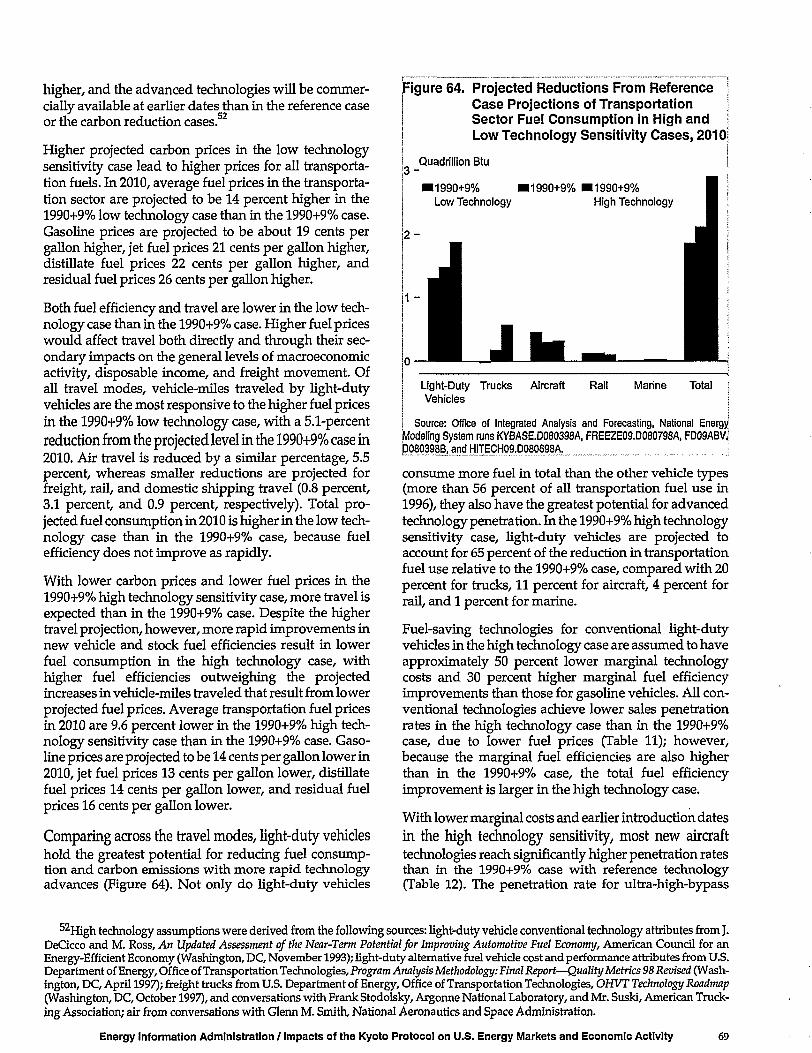
higher, and the advanced technologies will be commer-cially available at earlier dates than in the reference caseor the carbon reduction cases.52
Higher projected carbon prices in the low technologysensitivity case lead to higher prices for all transporta-tion fuels. In 2010, average fuel prices in the transporta-tion sector are projected to be 14 percent higher in the1990+9% low technology case than in the 1990+9% case.Gasoline prices are projected to be about 19 cents pergallon higher, jet fuel prices 21 cents per gallon higher,distillate fuel prices 22 cents per gallon higher, andresidual fuel prices 26 cents per gallon higher.
Both fuel efficiency and travel are lower in the low tech-nology case than in the 1990+9% case. Higher fuel priceswould affect travel both directly and through their sec-ondary impacts on the general levels of macroeconomicactivity, disposable income, and freight movement. Ofall travel modes, vehicle-miles traveled by light-dutyvehicles are the most responsive to the higher fuel pricesin the 1990+9% low technology case, with a 5.1-percentreduction from the projected level in the 1990+9% case in2010. Air travel is reduced by a similar percentage, 5.5percent, whereas smaller reductions are projected forfreight, rail, and domestic shipping travel (0.8 percent,3.1 percent, and 0.9 percent, respectively). Total pro-jected fuel consumption in 2010 is higher in the low tech-nology case than in the 1990+9% case, because fuelefficiency does not improve as rapidly.
With lower carbon prices and lower fuel prices in the1990+9% high technology sensitivity case, more travel isexpected than in the 1990+9% case. Despite the highertravel projection, however, more rapid improvements innew vehicle and stock fuel efficiencies result in lowerfuel consumption in the high technology case, withhigher fuel efficiencies outweighing the projectedincreases in vehicle-miles traveled that result from lowerprojected fuel prices. Average transportation fuel pricesin 2010 are 9.6 percent lower in the 1990+9% high tech-nology sensitivity case than in the 1990+9% case. Gaso-line prices are projected to be 14 cents per gallon lower in2010, jet fuel prices 13 cents per gallon lower, distillatefuel prices 14 cents per gallon lower, and residual fuelprices 16 cents per gallon lower.
Comparing across the travel modes, light-duty vehicleshold the greatest potential for reducing fuel consump-tion and carbon emissions with more rapid technologyadvances (Figure 64). Not only do light-duty vehicles
Figure 64. Projected Reductions From ReferenceCase Projections of TransportationSector Fuel Consumption in High andLow Technology Sensitivity Cases, 2010
Quadrillion Btu3 -
2 -
11990+9% •1990+9% ^1990+9%Low Technology High Technology
Light-Duty TrucksVehicles
Aircraft Rail Marine Total
Source: Office of Integrated Analysis and Forecasting, National EnergyModeling System runs KYBASE.D080398A, FREEZE09.D080798A, FD09ABV.'& C
consume more fuel in total than the other vehicle types(more than 56 percent of all transportation fuel use in1996), they also have the greatest potential for advancedtechnology penetration. In the 1990+9% high technologysensitivity case, light-duty vehicles are projected toaccount for 65 percent of the reduction in transportationfuel use relative to the 1990+9% case, compared with 20percent for trucks, 11 percent for aircraft, 4 percent forrail, and 1 percent for marine.
Fuel-saving technologies for conventional light-dutyvehicles in the high technology case are assumed to haveapproximately 50 percent lower marginal technologycosts and 30 percent higher marginal fuel efficiencyimprovements than those for gasoline vehicles. All con-ventional technologies achieve lower sales penetrationrates in the high technology case than in the 1990+9%case, due to lower fuel prices (Table 11); however,because the marginal fuel efficiencies are also higherthan in the 1990+9% case, the total fuel efficiencyimprovement is larger in the high technology case.
With lower marginal costs and earlier introduction datesin the high technology sensitivity, most new aircrafttechnologies reach significantly higher penetration ratesthan in the 1990+9% case with reference technology(Table 12). The penetration rate for ultra-high-bypass
^High technology assumptions were derived from the following sources: light-duty vehicle conventional technology attributes from J.DeCicco and M. Ross, An Updated Assessment of the Near-Term Potential for Improving Automotive Fuel Economy, American Council for anEnergy-Efficient Economy (Washington, DC, November 1993); light-duty alternative fuel vehicle cost and performance attributes from U.S.Department of Energy, Office of Transportation Technologies, Program Analysis Methodology: Final Report—Quality Metrics 98 Revised (Wash-ington, DC, April 1997); freight trucks from U.S. Department of Energy, Office of Transportation Technologies, OHVT Technology Roadmap(Washington, DC, October 1997), and conversations with Frank Stodolsky, Argonne National Laboratory, and Mr. Suski, American Truck-ing Association; air from conversations with Glenn M. Smith, National Aeronautics and Space Administration.
Energy Information Administration / Impacts of the Kyoto Protocol on U.S. Energy Markets and Economic Activity 69
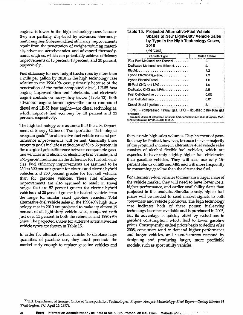
engines is lower in the high technology case, becausethey are partially displaced by advanced thermody-namic engines. Substantial fuel efficiency improvementsresult from the penetration of weight-reducing materi-als, advanced aerodynamics, and advanced thermody-namic engines, which can potentially achieve efficiencyimprovements of 15 percent, 18 percent, and 20 percent,respectively.
Fuel efficiency for new freight trucks rises by more than1 mile per gallon by 2010 in the high technology caserelative to the 1990+9% case, primarily because of thepenetration of the turbo compound diesel, LE-55 heatengine, improved tires and lubricants, and electronicengine controls on heavy-duty trucks (Table 13). Bothadvanced engine technologies—the turbo compounddiesel and LE-55 heat engine—are diesel technologies,which improve fuel economy by 10 percent and 23percent, respectively.
The high technology case assumes that the U.S. Depart-ment of Energy Office of Transportation Technologiesprogram goals for alternative-fuel vehicle cost and per-formance improvements will be met. Generally theseprogram goals include a reduction of 50 to 66 percent inthe marginal price difference between comparable gaso-line vehicles and electric or electric hybrid vehicles, anda 75-percent reduction in the difference for fuel cell vehi-cles. Fuel efficiency improvements are assumed to be230 to 300 percent greater for electric and electric hybridvehicles and 250 percent greater for fuel cell vehiclesthan for gasoline vehicles. These fuel efficiencyimprovements are also assumed to result in travelranges that are 57 percent greater for electric hybridvehicles and 20 percent greater for fuel cell vehicles thanthe range for similar sized gasoline vehicles. Totalalternative-fuel vehicle sales in the 1990+9% high tech-nology case in 2010 are projected to make up almost 19percent of all light-duty vehicle sales, compared withjust over 11 percent in both the reference and 1990+9%cases. The projected shares for different alternative-fuelvehicle types are shown in Table 15.
In order for alternative-fuel vehicles to displace largequantities of gasoline use, they must penetrate themarket early enough to replace gasoline vehicles and
Table 15. Projected Alternative-Fuel VehicleShares of Newby Type in the2010(Percent)
Vehicle Type
Flex-Fuel Methanol and Ethanol
Dedicated Methanol and Ethanol
Electric
Hybrid Electric/Gasoline
Hybrid Electric/Diesel
Bi-Fuel CNG and LPG .
Dedicated CNG and LPG
Fuel Cell Gasoline
Fuel Cell Methanol
Diesel Direct Injection
Light-Duty Vehicle SalesHigh Technology Cases,
| Sales Share9.12.11.21.31.61.02.50.020.01
2.1
CNG = compressed natural gas. LPG = liquefied petroleum gas(propane).
Source: Office of Integrated Analysis and Forecasting, National Energy Mod-eling System run KYBASE.D080398A.
then sustain high sales volumes. Displacement of gaso-line may be limited, however, because the vast majorityof the projected increase in alternative-fuel vehicle salesconsists of alcohol flexible-fuel vehicles, which areexpected to have only slightly higher fuel efficienciesthan gasoline vehicles. They will also use only 15-percent blends of E85 and M85 and will more frequentlybe consuming gasoline than the alternative fuel.
For alternative-fuel vehicles to maintain a larger share ofthe vehicle market, they will need to have lower costs,higher performance, and earlier availability dates thanprojected in this analysis. Simultaneously, higher fuelprices will be needed to send market signals to bothconsumers and vehicle producers. The high technologycase indicates both of these points: fuel-savingtechnology becomes available and is purchased in 2005,but its advantage is quickly offset by reductions ingasoline consumption, which lead to lower gasolineprices. Consequently, as fuel prices begin to decline after2008, consumers tend to demand higher performanceand larger vehicles, and manufacturers respond bydesigning and producing larger, more profitablemodels, such as sport utility vehicles.
53U.S. Department of Energy, Office of Transportation Technologies, Program Analysis Methodology: Final Report—Quality Metrics 98(Washington, DC, April 16,1997).
70 Enerc Information Administration / Im acts of the K oto Protocol on U.S. Enei. Markets and .

4. Electricity Supply
IntroductionThis chapter discusses the electricity supply side optionsunder various domestic carbon emissions reduc-tion cases, particularly the 24-percent-above-1990(1990+24%), 9-percent-above-1990 (1990+9%) and 3-percent-below-1990 (1990-3%) cases. The impacts onelectricity sector fuel use, capacity expansion and retire-ment decisions, electricity prices, and carbon emissionsare discussed. In addition, the results of sensitivity casesincorporating alternative assumptions about improve-ments in technology costs and performance, the poten-tial role for new nuclear power plants, and reducingimpacts on the coal industry are also discussed. Theeffects of demand-side decisions (i.e., consumer appli-ance choices and usage, as discussed in Chapter 3) thatwould reduce the demand for electricity are also con-sidered.
During the approximately 100-year history of theelectricity supply industry, the key fuels used to meetthe ever-increasing demand for electricity have changedas new generating technologies have emerged and fuelprices varied (Figure 65). Beginning with smallhydroelectric facilities just before the turn of the century,the industry then turned to fossil fuels. Among the fossilfuels, coal has almost always played a major role in U.S.electricity generation, and it remains the dominant fueltoday. Oil and natural gas use has varied, depending ontheir respective prices. In fact, concerns about future oiland natural gas prices contributed to the emergence ofnuclear power plants in the 1960s. In today's market,coal-fired power plants produce just over half of theelectricity used in the United States, nuclear plants 19percent, natural gas plants 14 percent, and hydroelectricplants about 10 percent. The remaining 7 percent comesfrom oil-fired plants and plants using other fuels such asmunicipal solid waste, wood, and geothermal and windpower.
In the reference case, which does not include the KyotoProtocol, the power generation sector is expected tobecome more energy-efficient over the next 20 years asnew, more efficient power plants are built. At the sametime, however, dependence on fossil fuels, especiallynatural gas and coal, is expected to increase, leading tosignificant growth in power plant carbon emissions.Coal is expected to remain the dominant fuel as existingplants are used more intensively, but generation from
Figure 65. Electricity Generation by Fuel in the| Reference Case, 1949-2020
Billion Kilowatthours
History
1950 1960 1970 1980 1990 2000 2010 2020.
Note: Data on nonutility generation are not available for years before[1989, but it was small. In 1989, nonutility generation accounted forJ6 percent of total U.S. electricity generation. II Sources: History: Energy Information Administration, Annual Energy Review1997, DOE/EIA-0384(97) (Washington, DC, July 1998). Projections: Office ofIntegrated Analysis and Forecasting, National Energy Modeling System runKYBASEpOSOSSSA
natural gas is expected to increase rapidly, with gas-fired plants making up the vast majority of new capacityadditions. Of the major non-carbon-based fuels,hydroelectric generation is expected to change verylittle, and nuclear generation is expected to decline asolder, more costly plants are retired. Looked at anotherway, while the efficiency of the generation sector,expressed as the amount of energy in terms of Britishthermal units (Btu) needed to produce each kilowatt-hour of electricity, is expected to improve, increasingdependence on fossil fuels will lead to more rapidgrowth in electricity sector carbon emissions than inelectricity sales (Figure 66). Without the improvement inefficiency, growth in fossil fuel use would match thegrowth in fossil-fired generation.
Although the costs of non-carbon-based generatingtechnologies have fallen, they still are not widely com-petitive with fossil fuel technologies. As a result, themost economical options available to electricity suppli-ers for meeting the demand for electricity over the next20 years are existing coal plants and new natural gasplants. In 1995, the average operating cost of coal-firedpower plants was 1.8 cents per kilowatthour. Only
Energy Information Administration / Impacts of the Kyoto Protocol on U.S. Energy Markets and Economic Activity 71
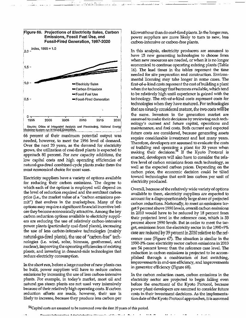
Figure 66. Projections of Electricity Sales, Carbon! Emissions, Fossil Fuel Use, andI Fossil-Fired Generation, 1997-2020
2 . 0 -
1.5-
1.0-
0 .5 -
Index, 1995 = 1.0
Electricity Sales
Carbon Emissions
Fossil Fuel Use
Fossil-Fired Generation
1995 2000 2005 2010 2015 2020
Source: Office of Integrated Analysis and Forecasting, National EnergyModeling System run KYBASE.D080398A. _ _ _ J
66 percent of their maximum potential output wasneeded, however, to meet the 1996 level of demand.Over the next 20 years, as the demand for electricitygrows, the utilization of coal-fired plants is expected toapproach 80 percent. For new capacity additions, thelow capital costs and high operating efficiencies ofnatural-gas-fired combined-cycle plants make them themost economical choice for most uses.
Electricity suppliers have a variety of options availablefor reducing their carbon emissions. The degree towhich each of the options is employed will depend onthe level of reduction required and the resultant carbonprice (i.e., the market value of a "carbon emissions per-mit") that evolves in the marketplace. Many of theoptions may require a significant financial incentive bef-ore they become economically attractive. Among the keycarbon reduction options available to electricity suppli-ers are reducing the use of relatively carbon-intensivepower plants (particularly coal-fired plants), increasingthe use of less carbon-intensive technologies (mainly
natural-gas-fired plants), the use of "carbon-free" tech-nologies (i.e. wind, solar, biomass, geothermal, andnuclear), improving the operating efficiencies of existingplants, and investing in demand-side technologies thatreduce electricity consumption.
In the short run, before a large number of new plants canbe built, power suppliers will have to reduce carbonemissions by increasing the use of less carbon-intensiveplants. For example, in today's market, most oil andnatural gas steam plants are not used very intensivelybecause of their relatively high operating costs. If carbonreduction efforts are made, however, their use islikely to increase, because they produce less carbon per
kilowatthour than do coal-fired plants. In the longer run,power suppliers are more likely to turn to new, lesscarbon-intensive or carbon-free plants.
In this analysis, electricity producers are assumed tohave 15 new generating technologies to choose fromwhen new resources are needed, or when it is no longereconomical to continue operating existing plants (Table16). The lead times in the tables represent the timeneeded for site preparation and construction. Environ-mental licensing may take longer in some cases. Thefirst-of-a-kind costs represent the cost of building a plantwhen the technology first becomes available, which tendto be relatively high until experience is gained with thetechnology. The nth-of-a-kind costs represent costs fortechnologies when they have matured. For technologiesthat are already considered mature, the two costs will bethe same. Investors in the generation market areassumed to make their decisions by reviewing each tech-nology's current and future capital, operations andmaintenance, and fuel costs. Both current and expectedfuture costs are considered, because generating assetsrequire considerable investment and last many years.Therefore, developers are assumed to evaluate tine costsof building and operating a plant for 30 years whenmaking their decisions. If the Kyoto Protocol isenacted, developers will also have to consider the rela-tive level of carbon emissions from each technology, aswell as the expected carbon prices. Depending on thecarbon price, the economic decision could be tiltedtoward technologies that emit less carbon per unit ofelectricity produced.
Overall, because of the relatively wide variety of optionsavailable to them, electricity suppliers are expected toaccount for a disproportionately large share of projectedcarbon reductions. Nationally, to meet an emissions tar-get 9 percent above 1990 levels, overall carbon emissionsin 2010 would have to be reduced by 18 percent fromtheir projected level in the reference case, which is 33percent above 1990 levels. But in order to meet the tar-get, emissions from the electricity sector in the 1990+9%case are reduced by 39 percent in 2010 relative to the ref-erence case (Figure 67). The situation is similar in the1990-3% case: electricity sector carbon emissions in 2010are 54 percent lower than the reference case level. Thereduction in carbon emissions is projected to be accom-plished through a combination of fuel switching,improvements in end-use efficiency, and improvementsin generator efficiency (Figure 68).
In the carbon reduction cases, carbon emissions in theelectricity sector are projected to begin falling evenbefore the enactment of the Kyoto Protocol, becausepower plant developers are assumed to consider futurecosts in their investment decisions. As the implementa-tion date of the Kyoto Protocol approaches, it is assumed
^Capital costs are assumed to be recovered over the first 20 years of this period.

Table 16. Cost and Performance Characteristics of New FossilGenerating Technologies
TechnologySize(MW)
LeadTime
(Years)
FirstElectricity
Date
OvernightCapital Costa
(1996 Dollarsper kWh)
First-of-a-Kind
nth-of-a-Kind
, Renewable, and Nuclear
VariableO&M
(1996 Millsper kWh)
Fixed O&M(1996
DollarsperkW)
Heat Rate(Btu per kWh)
First-of-a-kind
nth-of-a-Kind
CarbonEmissions(Poundsper MWh)
I Pulverized Coali (95% Scrubber)
I Advanced Coal(IGCC)
Oil/Gas Stream| (Conventional)
| Combined-Cyclej (Conventional, F-Frame) . . .
Combined-Cycle(Advanced, G- & H-Frame) .
Combustion Turbine(Conventional)
Combustion Turbine(Advanced Turbine System)Fuel Cell(Molten Carbonate)Nuclear (EvolutionaryAdvanced Reactor)
Biomass
Geothermalb
Municipal Solid Waste0
Solar Thermal
Solar Photovoltaic
Wind
400
380
300
250
400
160
120
10
1,3001005030100550
4
4
2
3
3
2
2
2
5441323
2001
2001
1998
2000
2000
1999
1999
2003
2010200519961995200019971997
1,079
1,833
991
440
572
325
458
2,189
2,356
2,243
NA
6,403
2,903
4,556
1,235
1,079
1,206
991
440
400
325
320
1,440
1,550
1,476
2,025
5,289e1,910e3,185
965
3.25
1.87
0.5
2.0
2.0
5.0
5.0
2.0
0.4
5.2
0.0
5.4
0.0
0.0
0.0
22.5
24.2
30.0
15.0
13.8
4.0
5.7
14.4
55.043.095.70.0
46.09.7
25.6
9,585
8,470
9,500
8,030
6,985
11,900
9,700
6,000
10,400
8,911
32,391
16,000
NA
NA
NA
9,087
7,308
9,500
7,000
6,350
10,600
8,000
5,361
10,4008,224
NA
16,000
NA
NA
NA
519
417
296
250
198
330
249
167
0000000
I ^Overnight capital cost plus project contingencies.I Because geothermal cost and performance parameters are specific for each of the 51 sites in the database, the value shown is an average for thecapacity built in 2000.
°Because municipal solid waste does not compete with other technologies in the model, these values are used only in calculating the averagecosts of electricity.j Solar thermal is assumed to operate economically only in Electricity Market Module regions 2,5, and 10-13, that is, West of the Mississippi River,because of its requirement for significant direct, normal insulation.! eCapital costs for solar technologies are net of (reduced by) the 10 percent investment tax credit.
kW = kilowatt. kWh = kilowatthour. MW = megawatt. MWh = megawatthour. NA = not available. O&M = operations and maintenance costs.j Sources: Most values are derived by the Energy Information Administration, Office of Integrated Analysis and Forecasting from analysis of reports and discussions with'yarious sources from industry, government, and the National Laboratories, with the following specific sources: Solar Thermal—California Energy CommissionMemorandum, Technology Characterization for ER94 (August 6, 1993). Photovoltaic—Electric Power Research Institute, Technical Assessment Guide, EPRI-TAG[1993. Municipal Solid Waste—EPRI-TAG 1993. J
that developers will incorporate their expectations ofcarbon prices into their plans for new capacity additions,and that more lower-carbon generating capacity will bebrought on line than would have been in the absence ofthe expected carbon reduction mandate.
Trends in Fuel Useand Generating Capacity
To reduce power plant carbon emissions in the 1990+9%case, the mix of fuels used to produce electricity isexpected to change significantly from historical patterns(Figure 69). The change required is possible, but it willbe challenging. For example, the shift required tostabilize carbon emissions 9 percent above 1990 levels is
unprecedented historically. Even during the 1960s and1970s, when nuclear generation grew rapidly, thechange in fuel use patterns was not as dramatic as wouldbe required in this case. In the 1990+24% case, the shift isless pronounced, but coal-fired generation still isprojected to be 17 percent lower in 2010 and 40 percentlower in 2020 than in the reference case. Across thecarbon reduction cases, the projections show aconsistent shift away from coal to natural gas andrenewables for electricity generation. In addition,nuclear generation remains near current levels, and thedemand for electricity falls as the carbon reduction goaltightens (Figure 70).
The shift away from coal-fired generation occursbecause coal accounts for such a large share of powerplant carbon emissions. In 1996, coal-fired power plants
Energy Information Administration / Impacts of the Kyoto Protocol on U.S. Energy Markets and Economic Activity 73

Figure 67. Projections of Carbon Emissions Fromthe Electricity Supply Sector, 1996-2020
Reference
1990+24%
90+9%
1990-3%
2010 2015 2020!
Source: Office of Integrated Analysis and Forecasting, National Energy'Modeling System runs KYBASE.D080398A, FD24ABV.D080398B, FD09ABV.D080398B, and FD03BLW.D080398B.
Figure 68. Projected Reductions in CarbonEmissions From the Electricity SupplySector, 1990-3% Case, 1996-2020
,600-
500-
J400-
i300-
Million Metric Tons
•Demand Reductions
I Generation Efficiency
I Fuel Switching
2000 2005 2010 2015 2020
Source: Office of Integrated Analysis and Forecasting, National EnergyModeling System runs KYBASE.D080398A and FD03BLW.D080398B. '
produced an estimated 92 percent of the carbon emis-sions in the power generation sector. In the referencecase, that share is expected to be 86 percent in 2010; andin 2020, even though natural-gas-fired generation growsrapidly, coal plants still are expected to account for 81percent of total carbon emissions from the electricity sec-tor. Per unit of fuel consumed (Btu), coal plants emitnearly 80 percent more carbon than do natural gasplants, and the difference is even greater per megawat-thour of electricity generated (Table 17). New naturalgas combined-cycle plants are much more efficient thanexisting coal plants, requiring less than two thirds theamount of fuel (in Btu) to produce a kilowatthour ofelectricity. As a result, per megawatthour of electricity
Figure 69. Electricity Generation by Fuel, 1990+9%Case, 1949-2020
5,000 -
4,000 -
Billion Kilowatthours
History Projections
•Renewable/OtherI 3 ' 0 0 0 " .Hydro
•Nuclear
!2,000- OO'1
•Gas•Coal
1,000-
1950 1960 1970 1980 1990 2000 2010 2020
. Note: Data on nonutility generation are not available for years beforet
[1989, but it was small. In 1989, nonutility generation accounted forJ6 percent of total U.S. electricity generation. j
Sources: History: Energy Information Administration, Annual Energy Review,1997, DOE/EIA-0384(97) (Washington, DC, July 1998). Projections: Office o^Integrated Analysis and Forecasting, National Energy Modeling System runFD09ABV.D080398B. j
Figure 70. Electricity Generation by Fuel, 2010S
Billion KilowatthoursIReference •1990+24% •1990+9% • ' ; & : >
j-1,000——
3
o•nuCD
inw•a=
n
•D
c
Wii
to
Ea^o
O
CDJO
6
• •ctoECDQ
CO
co
••JJ3
• o
a:
' Source: Office of Integrated Analysis and Forecasting, National EnergyModeling System runs KYBASE.D080398A, FD24ABV.D080398B, FD09ABVJ
produced, existing coal plants release nearly 3 times asmuch carbon into the atmosphere as do the most effi-cient new natural gas plants.
Coal
Generation
In the carbon reduction cases, the projected decreasesin coal-fired electricity generation are dramatic. In the1990+24%, 1990+9%, and 1990-3% cases, coal-firedgeneration in 2010 is expected to be 18 percent, 53percent, and 75 percent lower, respectively, than in the

Table 17. Carbon Emissions From Fossil Fuel Generating Technologies
Technology
Heat Rate(Btu per
Kilowatthour)
Carbon Emissions
Pounds perMillion Btu
Pounds perMegawatthour
Coal-Fired Technologies
Existing Capacity
New Capacity Additions
| Advanced Coal Technology
| Natural-Gas-Fired Technologies
I Conventional Turbine| Advanced Turbine
j Existing Gas Steam
j Conventional Combined-Cycle...
| Advanced Combined-Cycle
j Fuel Cell
10,0009,0877,308
10,6008,00010,3007,0006,3505,361
575757
323232323232
571519418
336253326222201170
i Source: Energy Information Administration, Office of Integrated Analysis and Forecasting.
reference case (Figure 71). In 2020, the differences fromthe reference case are even larger: 41 percent in the1990+24% case, 77 percent in the 1990+9% case, and over96 percent in the 1990-3% case. In 1990-3% case, coal-fired generation is virtually eliminated. Coal plantssimply are not very economical when carbon prices arehigh.
Such reductions in coal use would come at a cost.Although they are major carbon emitters, existing coalplants are very economical, and their operating costshave been falling (Figure 72). Under more stringentemissions reduction targets, however, with risingcarbon prices, the economics of coal-fired generationwould change (Table 18). For a power supplier decidingwhether to continue operating an existing coal plant,build a new coal plant, build a new natural-gas-firedcombined-cycle plant, or convert an existing coal-firedplant to natural gas, continued operation of the coalplant would be a clear winner in the absence of a carbonprice. As the carbon price rises, however, the newnatural gas plant looks more attractive. In thehypothetical example, assuming a 70-percent capacityfactor for the four types of plant, it would make sense toshut the coal plant down and build a new natural gasplant at a carbon price of approximately $100 per metricton of carbon. 5 Assuming a 30-percent capacity factor,the crossover point would be closer to $200 per metricton of carbon. In this hypothetical example, the carbonprices that would induce power suppliers to retireexisting coal plants are high, because the operating costsof most existing coal plants are low. In reality, thecrossover point would vary from plant to plant.
Generating Capacity
In all the carbon reduction cases, significant amounts ofcoal capacity are expected to be retired (Figure 73). Ingeneral, the projected changes in the mix of generating
Figure 71. Projections of Coal-Fired ElectricityGeneration, 2000-2020
2,500-,
:2,ooo -
1,500 -
1,000-
500-
Billion KilowatthoursIReference •1990+24% •1990+9% •1990-3%
2000 2005 2010 2015 2020! Source: Office of Integrated Analysis and Forecasting, National EnergyModeling System runs KYBASE.D080398A, FD24ABV.D080398B, FD09ABVJj !
capacity parallel the changes in fuel use. As the domesticcarbon reduction requirement becomes more stringent,more coal capacity is retired and more natural gas andrenewable plants are built (Figure 74). In the 1990+24%and 1990+9% cases, there is 3 percent and 10 percent lesscoal-fired capacity by 2010, and 13 percent and 36 per-cent less by 2020. Approximately two-thirds of the exist-ing coal-fired capacity is projected to be retired by 2020in the 1990-3% case. The net result is that the share ofcapacity accounted for by coal plants declines fromaround 40 percent in 1996 to just over 29 percent in 2010and to slightly over 11 percent in 2020 in the 1990-3%case.
One possible effect of the projected coal plant retire-ments is that some of the plants may be shut downbefore their total investment costs are recovered. Such
55In NEMS, the capacity factor for a particular plant type is determined by its operating costs. The values presented here are for illustra-tion only.
Energy Information Administration / Impacts of the Kyoto Protocol on U.S. Enej. Markets and Economic Activ

Table 18. Hypothetical Examples of Levelized Plant Costs at Various Carbon PricesI (1996 Cents per Kilowatthour)
Plant TypeCarbon Price (1996 Dollars per Metric Ton)
50 100 I 150 I 200 250 300
j 70-Percent Capacity Factor
Existing Coal-Fired
New Coal-Fired
New Gas-Fired Advanced Combined-Cycle
Coal-to-Gas Conversion
30-Percent Capacity Factor
Existing Coal-Fired
New Coal-FiredNew Gas-Fired Advanced Combined-Cycle
Coal-to-Gas Conversion
1.643.673.043.45
1.926.694.233.90
2.92
4.91
3.53
4.19
3.217.934.724.64
4.216.164.024.94
4.49
9.18
5.22
5.38
5.497.404.525.68
5.78
10.42
5.716.12
6.78
8.65
5.01
6.42
7.06
11.67
6.21
6.87
8.06
9.89
5.50
7.16
8.35
12.91
6.70
7.61
9.3511.146.007.91
9.63
14.16
7.19
8.35
Source: Energy Information Administration, Office of Integrated Analysis and Forecasting.
Figure 72. Operating Costs for Coal-Fired \Electricity Generation Plants, 1981-1995 j
1995 Mills per Kilowatthour j
•Fuel •Nonfuel !4 0 -
1983 1985 1987 1989
Source: Form FERC-1, "Annual Report of Major Electric Utilities, Licensees;and Other." j
unrecovered costs would be stranded. Most coal plantsare fairly old, however, and their construction costs havealready been recovered. On the other hand, some plantowners could suffer losses because plants they expectedto be profitable might no longer be profitable whencarbon prices are imposed.
Natural GasGeneration
The story for natural gas generation is the opposite ofthat for coal (Figure 75). As the requirement to reducecarbon emissions tightens and the associated carbonprice rises, natural-gas-fired generation becomes moreeconomical than coal-fired generation. In 2010 andbeyond, electricity generation from natural gas isbetween 17 percent and 76 percent higher in the carbonreduction cases than in the reference case projections.Overall, between 1996 and 2020, natural gas generationincreases by almost 500 percent in the most stringentcarbon reduction cases, and even in the 1990+24% case it
Figure 73. Projections of Coal-Fired GeneratingCapacity, 2000-2020
400-Gigawatts•Reference •1990+24% •1990+9% • 1990-3%
300-
200-
1100-
2000 2005 2010 2015 2020Source: Office of Integrated Analysis and Forecasting, National Energy
Modeling System runs KYBASE.D080398A, FD24ABV.D080398B, FD09ABVJ^ L W J
Figure 74. Electricity Generation Capacity by Fuel,2010
5 0 0 -
4 0 0 -
Gigawatts
BReference ^1990+24% "1990+9% 01990-3%
n
Coal Gas and Oil Hydro Other NuclearRenewables
Source: Office of Integrated Analysis and Forecasting, National EnergyModeling System runs KYBASE.D080398A, FD24ABV.D080398B, FD09ABVJP080398B, and FD03BLW.D080398B.
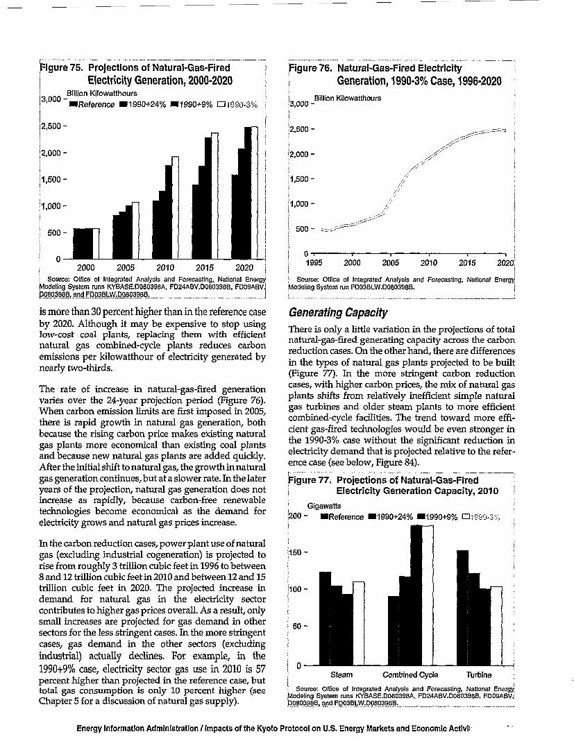
Figure 75. Projections of Natural-Gas-FiredElectricity Generation, 2000-2020
3,000 -Billion Kilowatthours j
•Reference •1990+24% •1990+9% £31980-3% i
2000 2005 2010Source: Office of Integrated Analysis and Forecasting, National Energy
/Modeling System runs KYBASE.D080398A, FD24ABV.D080398B, FD09ABVJB0B0398B, m
is more than 30 percent higher than in the reference caseby 2020. Although it may be expensive to stop usinglow-cost coal plants, replacing them with efficientnatural gas combined-cycle plants reduces carbonemissions per kilowatthour of electricity generated bynearly two-thirds.
The rate of increase in natural-gas-fired generationvaries over the 24-year projection period (Figure 76).When carbon emission limits are first imposed in 2005,there is rapid growth in natural gas generation, bothbecause the rising carbon price makes existing naturalgas plants more economical than existing coal plantsand because new natural gas plants are added quickly.After the initial shift to natural gas, the growth in naturalgas generation continues, but at a slower rate. In the lateryears of the projection, natural gas generation does notincrease as rapidly, because carbon-free renewabletechnologies become economical as the demand forelectricity grows and natural gas prices increase.
In the carbon reduction cases, power plant use of naturalgas (excluding industrial cogeneration) is projected torise from roughly 3 trillion cubic feet in 1996 to between8 and 12 trillion cubic feet in 2010 and between 12 and 15trillion cubic feet in 2020. The projected increase indemand for natural gas in the electricity sectorcontributes to higher gas prices overall. As a result, onlysmall increases are projected for gas demand in othersectors for the less stringent cases. In the more stringentcases, gas demand in the other sectors (excludingindustrial) actually declines. For example, in the1990+9% case, electricity sector gas use in 2010 is 57percent higher than projected in the reference case, buttotal gas consumption is only 10 percent higher (seeChapter 5 for a discussion of natural gas supply).
figure 76. Natural-Gas-Fired ElectricityGeneration, 1990-3% Case, 1996-2020
3,000 -
2,500 -
2,000 -
1,500-
1,000 -
5 0 0 -
Billion Kilowatthours
1995 2000 2005 2010 2015 2020:
I Source: Office of Integrated Analysis and Forecasting, National EnergyModeling System run FD03BLW.D080398B. I
Generating CapacityThere is only a little variation in the projections of totalnatural-gas-fired generating capacity across the carbonreduction cases. On the other hand, there are differencesin the types of natural gas plants projected to be built(Figure 77). In the more stringent carbon reductioncases, with higher carbon prices, the mix of natural gasplants shifts from relatively inefficient simple naturalgas turbines and older steam plants to more efficientcombined-cycle facilities. The trend toward more effi-cient gas-fired technologies would be even stronger inthe 1990-3% case without the significant reduction inelectricity demand that is projected relative to the refer-ence case (see below, Figure 84).rigure 77. Projections of Natural-Gas-Fired
Electricity Generation Capacity, 2010Gigawatts
200- •Reference ^1990+24% ^1990+9% •i99'}-3%
150-
100-
Sfeam Combined Cycle Turbine
Source: Office of Integrated Analysis and Forecasting, National Energy,Modeling System runs KYBASE.D080398A, FD24ABV.D080398B, FD09ABV,''D080398Rand FD03BLW.D080398B.
Energy Information Administration / Impacts of the Kyoto Protocol on U.S. Energy Markets and Economic Activil

A critical question is whether new natural gas capacitycan be built in sufficient quantity and in the right placesto reduce carbon emissions to the levels required by theKyoto Protocol. For example, in the 1990-3% case, theamount of capacity, mostly natural gas, projected to bebuilt in some years far exceeds the amount of capacitybuilt in any year since 1983. The average amount ofgenerating capacity brought on line each year since 1983has been around 10 gigawatts (33 typical plants).56 Thepeak year was 1985, when just under 22 gigawatts ofcapacity was added. In the 1990-3% case, annualadditions are projected to exceed 28 gigawatts (93typical plants) in some years.
Some gas-fired plants are expected to be built to meetgrowth in demand, but most are likely to replace retiringcoal plants. From 2008 to 2020, the projected additions ofgenerating capacity in the 1990-3% case average 24 giga-watts annually, with just over 28 gigawatts in 2009. Thislevel of construction is high but not unprecedented. It isactually less than the amount of capacity that was builtannually during the 1970s, when the demand for elec-tricity was growing at more than twice the rate projectedin the reference case.
Given time and forewarning, the natural gas plantdesign and construction industry should be able to meetthe challenge presented in the carbon reduction cases;however, the prices for new gas-fired facilities might riseabove those used in this analysis. In addition, the situa-tion could be exacerbated by the fact that many othercountries may also be turning to natural gas in order toreduce their carbon emissions.
Not only will a large number of new natural gas plantshave to be built, they will also have to be built in the rightplaces. Today's electricity transmission system is con-structed around major load and supply centers, connect-ing major cities to major power plants. The location ofpower plants is critical to the reliability of the electricitysupply system. If, as expected, a large number of exist-ing coal plants are retired to reduce carbon emissions,many of the new gas plants will have to be built at thelocations of the coal plants they replace, in order tomaintain the reliability of the system. (Biomass andwind plants must be built where their resources areavailable.) The alternative would be to reconfigure thetransmission system to accommodate new plant loca-tions,57 an undertaking that might require additionalinvestment.
One option for adding new natural-gas-fired capacitywould be to modify existing coal-fired plants to burnnatural gas instead of coal. This option, however, maynot prove to be economical. Generally, there are twoapproaches for converting a coal plant to burn gas. Thefirst is simply to modify the existing coal boiler so that itcan be fired with natural gas. From a mechanical per-spective this is not terribly difficult or expensive. Therequired plant modifications would be expected to cost$70 to $80 per kilowatt of capacity, mainly for new burn-ers and gas handling equipment (compressors, meteringstation, distribution headers, etc.). In terms of perform-ance, there would be a small loss of efficiency, 2 to 5 per-cent, if gas were burned in a boiler originally designed toburn coal.58
The main problem with this approach to plant conver-sion is the relative thermal inefficiency of existing coalplants. The majority of older coal plants consumebetween 10,000 and 10,500 Btu of fuel for each kilowat-thour of electricity they produce,59 as compared with6,500 to 7,500 Btu of fuel input for each kilowatthour ofelectricity produced by a new gas-fired combined-cycleplant. Existing coal plants are economical because thefuel is inexpensive, not because they are thermally effi-cient.
As described above (see Table 18), in the absence ofrequired carbon emissions reductions, existing coal-fired plants are the most economical option for electric-ity generation. Conversion of existing plants from coalto gas is not the most economical option if the plant is tobe used at a high capacity factor. If the price of carbonemissions rises, however, continuing to run the existingcoal plant becomes less economical. Assuming a 70-percent capacity factor and a carbon price of $100 permetric ton, it would make sense to abandon the plant(not the site) and build a new gas-fired combined-cycleplant. At a lower capacity factor, the carbon price wouldhave to be higher before the operational cost savingsfrom the greater efficiency of a new combined-cycleplant would offset its higher capital costs (Table 18).
The second approach to using gas in an existing coalplant would be to "repower" it by converting it into anatural gas combined-cycle plant. This approach wouldresult in higher plant efficiency, but it would also bemuch more expensive than the first approach. In a typi-cal repowering, the coal handling system and the boilerare replaced with new combustion turbines and a heat
56Depending on the technology type, new power plants differ tremendously in size, from a few kilowatts for the smallest distributedphotovoltaic technologies to 500,000 kilowatts (500 megawatts) or more for the largest new coal and nuclear technologies. Throughout thisreport, when a number of typical plants is provided, a 300-megawatt average plant size is used.
57See Energy Information Administration, "An Exploration of Network Modeling: The Case of NEPOOL," in Issues in Midterm Analysisand Forecasting 1998, DOE/EIA-0607(98) (Washington, DC, July 1998), for a discussion of the impact of plant location on reliability and pric-ing.
^Cost and performance impact estimates provided by Parsons Engineering.59Energy Information Administration, Form EIA-860, "Annual Electric Generator Report."
7 -1 . , ' ' ' •• " 1 . i . i. cts of the U 'oto Protocol on U.S. Eneri Markets and Economic Activit

recovery boiler. The only significant part of the plantthat is maintained is the original turbine generator. Thisapproach can be attractive at some facilities, but it is notwithout problems. New combined-cycle plants arepackaged systems. The turbines, heat recovery boiler,and turbine generator are designed to work smoothlytogether for optimal efficiency. Because many oldercoal-fired plants were custom designed and built, theydo not always come in standard sizes or configurationsor with standard operational parameters. If such facili-ties are to be repowered, additional work will berequired to integrate the system components. Given thatfor a typical combined-cycle plant the steam turbinegenerator accounts for between 10 and 22 percent of thecapital cost of the plant,60 the additional work could eas-ily drive the cost of repowering beyond what it wouldcost simply to replace the plant with a new, more effi-cient packaged combined-cycle plant.
Renewable FuelsIn the carbon reduction cases, U.S. electricity suppliersare expected to turn to renewable energy resources laterin the projection period to meet the demand forelectricity while reducing carbon emissions. Wind,biomass, geothermal, solar, and hydropower resourcesgenerally are thought to have less environmental impactthan fossil fuels; they are domestically available; and insome instances they have begun to penetrate U.S.electricity markets. Significant growth in the use ofnonhydroelectric renewable resources for electricitygeneration is expected to accompany efforts to reducecarbon emissions (Figure 78).
Figure 78. Projections of NonhydroelectricRenewable Electricity Generation,2000-2020
600 -
5 0 0 -
4 0 0 -
Billion Kilowatthours
Reference1990+24%1990+9%
2000 2005 2010 2015 2020
Source: Office of Integrated Analysis and Forecasting, National EnergyModeling System runs KYBASE.D080398A, FD24ABV.D080398B, FD09ABVJ
B F L y W j
The largest increases in renewable generation are ex-pected after 2010 in the most stringent carbon reductioncases (Table 19). For this reason, the results of the 7-percent-below-1990 (1990-7%) case are also discussed inthis section. Before 2010, nonhydroelectric renewabletechnologies generally are not competitive with newnatural gas plants, but their costs are expected to fallover time. With higher carbon prices, these technologiescan be expected to play a significant role in reducing car-bon emissions. In the reference case little growth in gen-eration from renewables is expected. In the carbonreduction cases, nonhydroelectric renewable generationis 1.1 to 1.7 times the reference case level in 2010 and 1.5to 4.8 times the reference case level in 2020.
Because of the lack of market experience with renewabletechnologies other than hydropower, there is consider-able uncertainty about the costs of developing them onthe scale that would be needed for large carbon emissionreductions. It is also unclear whether electric system reli-ability can be maintained if large quantities of wind orsolar, which have intermittent output, are developed.Although some environmental objections have beenraised against some renewables, including negativeeffects on animal life, destruction of habitat, and damageto scenery and recreation, these effects are small in com-parison with the alternatives. While wind and biomasstechnologies are expected to be the most importantrenewable technologies used to reduce carbon emis-sions, others—including geothermal, conventionalhydroelectric, and solar power plants—may also play arole (Table 19).
WindAmong the nonhydroelectric renewable fuels, biomassand wind technologies are expected to make the mostsignificant contributions to carbon emission reductions.Projected growth in the wind and biomass industries,together with the natural gas industry, would at leastpartially offset the impacts of declines in the coal indus-try. The biomass industry in the United States today issmall, but it could see large growth. Similarly, the windindustry, estimated to employ 30,000 to 35,000 peopleworldwide in 1995, could increase several times over inthe most stringent carbon reduction cases. In someregions, wind is projected to provide a significant shareof electricity supply. However, the ability of windresources to meet large-scale U.S. electric power needsreliably and cost-effectively is uncertain. Wind power isan intermittent technology, available only part of thetime during a day or season. As a result, EIA assumesthat the maximum contribution of wind power will belimited to 12 percent of any region's total annual genera-tion requirements (excluding cogeneration) to avoidreliability problems that larger shares might cause.
60Electric Power Research Institute, Technical Assessment Guide. The steam turbine and auxiliary systems account for 10 percent of theplant. If the boiler can also be used, this figure rises to 22 percent.
Energy Information Administration / Impacts of the Kyoto Protocol on U.S. Energy Markets and Economic Activity 79
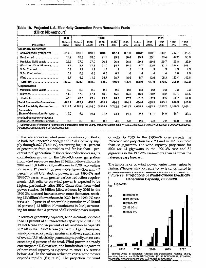
Table 19. Projected U.S. Electricity Generation From Renewable(Billion Kilowatthours)
ProjectionElectricity Generators
Conventional Hydropower
Geothermal
Municipal Solid Waste..Wood and Other BiomassSolar Thermal
Solar Photovoltaic
Wind
SubtotalCogenerators
Municipal Solid Waste
Biomass
Subtotal
Total Renewable Generation . .
Total Electricity Generation . . .
RenewableShare of Generation (Percent) . .
Nonhydroelectric RenewableShare of Generation (Percent) . .
2000Refer-ence
310.3
17.2
2288.20 9
0.1
5.7365 2
2.2
41.2
43.5
408.7
3,716.8
11.0
2.6
! Fuels
2010Refer-ence
313.0
16.8
27.08.71.2
0.6
6.2373 5
2.3
47.3
49.6
423.1
4,267.6
9.9
2.6
1990+24%
313.0
18.0
27 017.6
1 2
0.6
11.2
388 6
2 3
47 4
49.7
438.34,144.0
10.6
3.0
1990+9%
313.0
21.7
26 821.0
1 2
0.6
24.7
409 0
2.3
46 9
49.2
458.2
3,929.7
11.7
3.7
1990-3%
317.4
29.9
26 534.7
1 2
0.7
35.7
4461
2 3
45 9
48.2
494.3
3,712.6
13.3
4.8
1990-7%
321.9
30.4
26 536.4
1 2
1.0
48.9
466 2
2 3
456
47.9
514.1
3,641.7
14.1
5.3
2020Refer-ence
313.2
19.9
29 88.71.5
1.4
8.7
383 2
2 3
48 9
51.2
434.4
4,648.2
9.3
2.6Source: Office of Integrated Analysis and Forecasting, National Energy Modeling System runs KYBASE.D080398A,
FD03BLW.D080398B, and FD07BLW.D080398B.
1990+24%
313.1
25.1
29 822.5
1 5
1.443.6
437 0
2 3
50 2
52.5
489.5
4,422.3
11.1
4.0
1990+9%
313.1
33.4
29.783.1
1.5
1.4108.3
570 5
2.3
50.2
52.5
623.1
4,282.7
14.5
7.2FD24ABV.D080398B,
1990-3%
317.7
47.2
29.8244.4
1.5
1.8
123.4
765.9
2.3
50.4
52.7
818.5
4,160.2
19.7
12.0
1990-7%
322.4
53.3
29.9305.1
1.5
2.3
142.8
857.2
2.3
50.5
52.8
910.0
4,105.1
22.2
14.3FD09ABV.D080398B,
In the reference case, wind remains a minor contributorto both total renewable energy and total electricity sup-ply through 2020 (Table 19), accounting for just 2 percentof generation from renewables and far less than 1 per-cent of total generation. In the carbon reduction cases, itscontribution grows. In the 1990+9% case, generationfrom wind resources reaches 25 billion kilowatthours in2010 and 108 billion kilowatthours in 2020, accountingfor nearly 17 percent of renewable generation and 2.5percent of all U.S. electric power. In the 1990-3% and1990-7% cases, with greater carbon reduction require-ments, U.S. reliance on wind power is expected to behigher, particularly after 2010. Generation from windpower reaches 36 billion kilowatthours by 2010 in the1990-3% case and increases even more thereafter, reach-ing 123 billion kilowatthours in 2020. In the 1990-7% caseit rises to 10 percent of renewable generation in 2010 and16 percent (143 billion kilowatthours) in 2020, account-ing for more than 3 percent of all electric power output.
In terms of generating capacity, wind accounts for morethan 11 percent of all renewables capacity in 2010 in the1990-3% case and 26 percent of all renewables capacityin 2020 in the 1990-7% case (Table 20). Again, however,wind-powered capacity remains a relatively small shareof overall U.S. electricity generating capacity, in no caseexceeding 6 percent of the total. Wind power is alreadyentering some U.S. markets, and hundreds of megawattsof new wind capacity is expected to enter U.S. servicebefore 2000. In the carbon reduction cases, wind powerexpands rapidly (Figure 79). The projection for wind
capacity in 2005 in the 1990+9% case exceeds thereference case projection for 2020, and in 2020 it is morethan 38 gigawatts. The wind capacity projections for2020 are 44 gigawatts in the 1990-3% case and 51gigawatts in the 1990-7% case—more than 14 times thereference case forecast.
The importance of wind power varies from region toregion. Whereas wind capacity today is concentrated in
Figure 79. Projections of Wind-Powered Electricity;Generation Capacity, 2000-2020
6 0 -
| 5 0 -
4 0 -
130 -
Gigawatts
• Reference
• 1990+24%
• 1990+9%• 1990-3%• 1990-7%
Source: Office of Integrated Analysis and Forecasting, National EnergyModeling System runs KYBASE.D080398A, FD24ABV.D080398B, FD09ABVJD080398B, FD03BLW.D080398B, and FD07BLW.D080398B. J
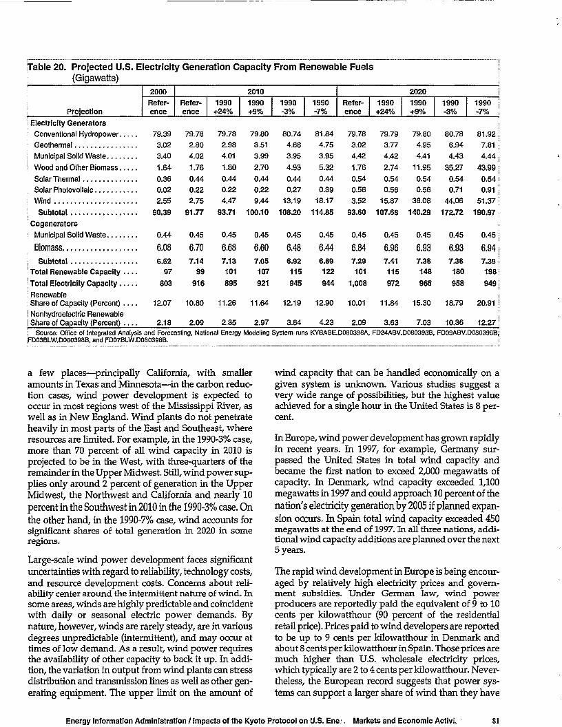
Table 20. Projected U.S. Electricity Generation Capacity(Gigawatts)
Projection
Electricity GeneratorsConventional Hydropower
Geothermal
Municipal Solid Waste
Wood and Other Biomass
Solar Thermal
Solar Photovoltaic
Wind
Subtotal
Cogenerators
Municipal Solid Waste
BiomassSubtotal
Total Renewable Capacity
Total Electricity Capacity
RenewableShare of Capacity (Percent)
Nonhydroelectric RenewableShare of Capacity (Percent)
2000
Refer-ence
From Renewable Fuels
2010
Refer-ence
79.39 79.78
3.02 2.80
3.40 4.02
1.64 1.76
0.36 0.44
0.02 0.22
2.55 2.75
90.39 91.77
0.44 0.45
6.08 6.70
6.52 7.1497 99
803 916
12.07 10.80
2.18 2.09
1990+24%
79.78
2.98
4.01
1.80
0.44
0.22
4.47
93.71
0.45
6.68
7.13101
895
11.26
2.35
1990+9%
79.80
3.51
3.99
2.70
0.44
0.22
9.44
100.10
0.45
6.60
7.05107
921
11.64
2.97
1990-3%
80.74
4.68
3.95
4.93
0.44
0.27
13.19
108.20
0.45
6.48
6.92
115
945
12.19
3.64
1990-7%
81.84
4.75
3.95
5.32
0.44
0.39
18.17
114.85
0.45
6.44
6.89122
944
12.90
4.23
2020
Refer-ence
1990+24%
79.78 79.79
3.02 3.77
4.42 4.42
1.76 2.74
0.54 0.54
0.56 0.56
3.52 15.87
93.60 107.68
0.45 0.45
6.84 6.96
7.29 7.41101 115
1,008 972
10.01 11.84
2.09 3.63
1990+9%
79.80
4.95
4.41
11.95
0.54
0.56
38.08
140.29
0.45
6.93
7.38148
965
15.30
7.03', Source: Office of Integrated Analysis and Forecasting, National Energy Modeling System runs KYBASE.D080398A, FD24ABV.D080398B,FD03BLW.D080398B, and FD07BLW.D080398B.
1990-3%
80.78
6.94
4.43
35.27
0.54
0.71
44.06
172.72
0.45
6.93
7.38180
958
18.79
10.36
1990-7%
81.92
7.81
4.44
43.99
0.54
0.91
51.37
190.97
0.45
6.94
7.39198
949
20.91
12.27FD09ABV.D080398B,
a few places—principally California, with smalleramounts in Texas and Minnesota—in the carbon reduc-tion cases, wind power development is expected tooccur in most regions west of the Mississippi River, aswell as in New England. Wind plants do not penetrateheavily in most parts of the East and Southeast, whereresources are limited. For example, in the 1990-3% case,more than 70 percent of all wind capacity in 2010 isprojected to be in the West, with three-quarters of theremainder in the Upper Midwest. Still, wind power sup-plies only around 2 percent of generation in the UpperMidwest, the Northwest and California and nearly 10percent in the Southwest in 2010 in the 1990-3% case. Onthe other hand, in the 1990-7% case, wind accounts forsignificant shares of total generation in 2020 in someregions.
Large-scale wind power development faces significantuncertainties with regard to reliability, technology costs,and resource development costs. Concerns about reli-ability center around the intermittent nature of wind. Insome areas, winds are highly predictable and coincidentwith daily or seasonal electric power demands. Bynature, however, winds are rarely steady, are in variousdegrees unpredictable (intermittent), and may occur attimes of low demand. As a result, wind power requiresthe availability of other capacity to back it up. In addi-tion, the variation in output from wind plants can stressdistribution and transmission lines as well as other gen-erating equipment. The upper limit on the amount of
wind capacity that can be handled economically on agiven system is unknown. Various studies suggest avery wide range of possibilities, but the highest valueachieved for a single hour in the United States is 8 per-cent.
In Europe, wind power development has grown rapidlyin recent years. In 1997, for example, Germany sur-passed the United States in total wind capacity andbecame the first nation to exceed 2,000 megawatts ofcapacity. In Denmark, wind capacity exceeded 1,100megawatts in 1997 and could approach 10 percent of thenation's electricity generation by 2005 if planned expan-sion occurs. In Spain total wind capacity exceeded 450megawatts at the end of 1997. In all three nations, addi-tional wind capacity additions axe planned over the next5 years.
The rapid wind development in Europe is being encour-aged by relatively high electricity prices and govern-ment subsidies. Under German law, wind powerproducers are reportedly paid the equivalent of 9 to 10cents per kilowatthour (90 percent of the residentialretail price). Prices paid to wind developers are reportedto be up to 9 cents per kilowatthour in Denmark andabout 8 cents per kilowatthour in Spain. Those prices aremuch higher than U.S. wholesale electricity prices,which typically are 2 to 4 cents per kilowatthour. Never-theless, the European record suggests that power sys-tems can support a larger share of wind than they have
Energy Informatfon Administration / Impacts of the Kyoto Protocol on U.S. Ene Markets and Economic ActivL ' 81

in the United States to date and that, if prices are highenough, capacity can be added fairly rapidly/61
A second issue is the considerable uncertainty sur-rounding the future cost of wind turbines. Installed capi-tal costs for wind turbines and associated equipmenthave fallen over the past 20 years and are expected tocontinue falling, particularly if large numbers of tur-bines are built. The costs are near $1,000 per kilowatt ofwind capacity today, and they are projected to be below$800 per kilowatt early in the 21st century and toapproach $600 per kilowatt by 2020 in the most stringentcarbon reduction cases. With no known manufacturingbarriers to large increases in factory production capacityfor wind turbines, the industry should be able to meetthe production levels called for in the carbon reductioncases, given sufficient lead times. Of course, it is impos-sible to say with certainty that the projected cost declineswill occur. This analysis does adjust for the cost effects ofshort-term bottlenecks in identifying sites, permittingprojects, manufacturing equipment, and installing proj-ects, but the actual effects of rapid large-scale expansionare not known.
While there appear to be large wind resources in manyregions, the costs of developing some of the sites may behigh. In general, wind power costs are expected toincrease as the best natural resources are consumed andless-favored sites enter service. Lower quality sites—including those on steep, rocky, or sharply variedsurfaces, those in more difficult environments (excessivecold, moisture, dirt, insects, or storms), and those withless useful winds (unpredictable, ill-timed, sharplyvarying, too fast)—could have much higher costs thanmore favorable sites. Moreover, in most regions only aportion of the total potential is likely to be economical.The possible stress on wind resources (and thereforecosts) can be seen by comparing projections of windcapacity with EIA's estimates of "economic" re-sources—identified as those available at capital costs no
more than double the baseline projection (Figure 80). Inthe 1990-7% case, eight regions consume a third or moreof "economic" wind resources, and three regions exceedthat portion of supply, including California. In thoseregions, more expensive wind resources are developedin the most stringent carbon reduction cases. Little isknown about the actual costs at these levels of resourceuse.62
The costs of transmission interconnections and ofupgrading existing distribution and transmissionnetworks are also expected to increase as the penetrationof wind resources grows. As projects are developed atgreater distances from existing lines, the costs of new
Figure 80. Projected Shares of Most EconomicalWind Resources Developed by Region,1990-7% Case, 1996-2020
Percent
sHI
o
Note: ECAR=East Central Area Reliability Coordination AgreementRegion; ERCOT = Electric Reliability Council of Texas; MAAC = Midi•Atlantic Area Council; MAIN = Mid-America Interconnected Network;'MAPP = Mid-Continent Area Power Pool; NY = New York Power Pool!HE = New England Power Pool; FL = Florida subregion of the South-eastern Electric Reliability Council; STV = Southeastern Electric Relitability Council excluding Florida; SPP=Southwest Power Pool; NWP =Northwest Pool subregion of the Western Systems Coordinating!Council; RA = Rocky Mountain and Arizona-New Mexico Power Areas?*CNV = California-Southern Nevada Power Area. ]
Source: Office of Integrated Analysis and Forecasting, National Energy Mod-j'sling System run FD07BLW.D080398B. j
interconnections will increase. In addition, the costs ofupgrading existing local distribution networks, both totransmit the electricity generated from wind power andto offset the destabilizing local effects of varying powerflows, will increase.
Finally, market competition for land with good windresources is also likely to increase the future costs ofextensive wind power development. Other urban oragricultural uses may compete for some locations. Publi-c opposition to wind project development on environ-mental, cultural, and recreational grounds may alsogrow as large numbers of wind facilities are built.Because excellent wind resources tend to occur in highlyvisible places, such as along ridges and other naturalprojections, preferred sites often serve other cultural,scenic, or religious purposes, and they may not be madeavailable for wind power development. For example, itremains to be seen whether the development of 170square miles in Texas (about 0.1 percent of the land area)for the wind capacity that would be needed to meet the2020 projections in the 1990-7% case would be accept-able to the State's inhabitants.
6 1 American Wind. Energy Association, International Wind Energy Capacity Projections (Washington, DC, April 1998).62Only 6 percent of the estimated, wind resources in region 5 (including Minnesota, Iowa, and the Dakotas) are used in the 1990-7% case;
however, the remaining resources are not economically accessible to other regions.

BiomassUnlike wind plants, which are intermittent, biomassplants operate continuously. Biomass currently is beingused to supply energy for power generation and in theindustrial, transportation, and residential sectors. Thelargest amount of biomass is used in the paper and lum-ber industries, where residue is burned to produce bothelectricity and steam (cogeneration). Biomass is alsoused to produce ethanol for fuel in the transportationsector, and wood is burned for residential heating.
Current biomass consumption in the electricity sector,excluding cogeneration, is limited to a few inefficientwood-burning generating units and a small amount ofcofiring at coal plants. Newer technologies, primarilyseveral types of gasification combined-cycle units, are inthe demonstration phase in the United States and areexpected to be commercially available by 2005. Suchunits would be somewhat more expensive than currenttechnology, but they are expected to be more than twiceas efficient. They can use a variety of fuel sources, suchas wood and wood residues, several types of energycrops, and crop residues. Without a carbon price, thesefacilities currently are not competitive with new naturalgas or coal plants. However, using biomass in the pro-duction of electricity produces no net carbon emissions.The carbon emitted during biomass combustionapproximates the carbon sequestered during the growthof the trees or crops that are burned. As a result, it is anattractive option for complying with the Kyoto Protocol.
In the 1990+24% case, biomass generation increases onlyslightly from the levels projected in the reference case. Inthe 1990+9% case, however, biomass generation is pro-jected to reach 68 billion kilowatthours—21 percentabove the reference case projection—in 2010 and 133 bil-lion kilowatthours—more than double the referencecase projection—in 2020. In the 1990-3% case, biomassgeneration is projected to be 81 billion kilowatthours in2010—44 percent above the reference case—and 295 bil-lion kilowatthours—5.0 times the reference case—in2020. And in the 1990-7% case, biomass generationexceeds the reference case projection by about 47 percentin 2010 and by 6.2 times in 2020. In each of these cases,biomass is allowed to contribute up to 5 percent of a coalplant's fuel input, but because coal plant usage declinesrapidly as the carbon price increases, the contributionfrom cofiring is limited.
With biomass resources projected to play such a majorrole in meeting electricity needs in the carbon reductioncases, a critical question is whether the projected levelsof reliance on biomass would be realistic. To answer thatquestion, it is necessary to examine the components ofthe biomass resource. Biomass resources are diverse andpotentially much larger than the amounts projected tobe developed even in the most stringent carbonreduction cases in this analysis (Figure 81).
Figure 81. Estimated Biomass ResourceAvailability and Projected GeneratingCapacity in 2020 by Region
Gigawatts6 0 ' •Reference •1990+24% •1990+9% 01990-3%
SO
J40
J30
2 0
ko
•Resource
JJ s rJ J J O U U J JK. H< oo o
UJ
o 2 2-
i IUJ
z OccUJCO
Q. Q.
8t 5 o
Note: ECAR = East Central Area Reliability Coordination AgreementRegion; ERCOT = Electric Reliability Council of Texas; MAAC = MidAtlantic Area Council; MAIN = Mid-America Interconnected Network;MAPP = Mid-Continent Area Power Pool; NY = New York Power Pool;WE = New England Power Pool; FL = Florida subregion of the Southfeastem Electric Reliability Council; STV = Southeastern Electric Reli-Iability Council excluding Florida; SPP = Southwest Power Pool; NWP =Northwest Pool subregion of the Western Systems CoordinatingjCouncil; RA = Rocky Mountain and Arizona-New Mexico Power Areas;,CNV = California-Southern Nevada Power Area.( Source: Office of Integrated Analysis and Forecasting, National EnergyModeling System runs KYBASE.D080398A, FD24ABV.D080398B, FD09ABV.'D080398B, FD03BLW.D080398B, and FD07BLW.D080398B.
Biomass materials are derived from a variety of sources,including urban wood waste, mill residues, forest resi-due, agricultural residue, and energy crops grown spe-cifically for combustion. Urban wood waste includestree trimmings, construction and demolition debris, anddiscards such as crates and pallets. (Some of these mate-rials are currently being used to make recycled productsor as fuel, and the resource data used for this analysisexclude those quantities.) Mill residues are the sawdustand scrap from sawmills, pulp mills, and wood productfacilities. Many mill residues are consumed on site, butsome are accumulated in stockpiles or sent to landfills,often at a cost to the producer. Forest residues are, gener-ally, material that is too low grade to be used for otherproducts. They include branches, dead trees, unmarket-able species, and cull trees from commercial forests. Thealternative to its use as a fuel is to leave it in the forest.Agricultural residues include a wide variety of materi-als. The greatest quantities (and the only amountsincluded in this analysis) are from wheat straw andcornstalks. Only a small amount is currently used asfuel, most being left in the field. It is assumed here thatonly 40 percent of all agricultural residues would beavailable for use as fuel, with the rest continuing to beleft in the field. What the above types of residues have incommon is that they are very inexpensive at the source.On the other hand, the cost of gathering and deliveringthem to a power plant, compared with the cost of coal,
Energy Information Administration / Impacts of the Kyoto Protocol on U.S. Energy Markets and Economic Activity 83

visually makes them too expensive for use in electricitygeneration under current economic conditions.
Energy crops involve dedicated operations that wouldlikely require long-term agreements between growersand conversion plant operators. The primary energycrops are willow, poplar, and switchgrass, each with dis-tinct growing areas and conditions. Energy crops differfrom residues in that it is the cost of growing them, notcollection, that dominates their total costs.
Agricultural lands can be divided into croplands, pas-turelands, and Conservation Reserve Program (CRP)acreage. The total U.S. agricultural land supply isapproximately 960 million acres, of which about one-third is now used for field crops. In some instances,energy crops can be grown on poor quality land that hasno other use. The amounts of agricultural land assumedto be available for energy crops in the resource data usedfor this analysis include all the CRP acreage, 20 percentof the cropland, and 10 percent of the pastureland. How-ever, even in the cases that project the highest levels ofbiomass use, the total amount of land needed for energycrops would be about 10 to 12 million acres, which is inthe range of the yearly fluctuations of U.S. croplandplanted. Thus, the question of competition for land doesnot appear large. As fossil fuel prices rise in the morestringent carbon reduction cases, the value of biomassfuels would also rise, making energy crops more attrac-tive economically.
There may be competition between the use of land forbiomass energy crops and its use for tree planting toincrease carbon sequestration. In terms of the amount ofcarbon sequestered or emissions avoided per acre ofland used, displacing a new gas-fired plant with abiomass-fired plant would have about the same impactas planting trees. For example, the U.S. EnvironmentalProtection Agency estimates that planting 1 acre of treeson marginal land would sequester 0.6 to 1.6 metric tonsof carbon annually.63 In comparison, if a new biomasspower plant displaced a new gas-fired plant, an esti-mated 1.3 metric tons of carbon emissions would beavoided per acre of land used.64 The comparison wouldnot be as close if the generation displaced were from acoal-fired power plant, which would emit roughly 3metric tons of carbon in producing the same amount ofelectricity that a biomass plant would generate from 1acre of crops. The critical issue in the land use decisionbetween tree planting and energy crops will be the rela-tive economics of the two choices. If sequestrationproves to be more economical, fewer biomass plantsmay be built than projected in this analysis. Instead of
building a biomass plant, a developer could simplybuild a gas-fired plant and also grow enough trees to off-set the carbon emissions from the plant.
It is assumed in this analysis that energy crops will notbecome economical until new integrated gasificationcombined-cycle (IGCC) plants are available in 2005 andafter. The current technology for biomass plants, usingstoker boilers, is inefficient and uneconomical. Thenewer IGCC technology is now being tested, and it isexpected to be vastly superior to the current technologyin terms of both efficiency and emissions. Most of theexperience with the IGCC technology has been inEurope, particularly in Scandinavia. Sydkraft, thesecond-largest utility in Sweden, has been operating a 6-megawatt wood-fired IGCC plant in Varnami, Sweden,since 1994. Finland has a 30-megawatt unit operating onwood waste, as well as several smaller peat-fired gasifi-cation units with a combined capacity of 50 megawatts.There are several other demonstration plants that totalabout 5 megawatts of capacity worldwide. Future plansinclude 12 megawatts of capacity in Italy (Bioelettrica), 8megawatts in the United Kingdom, and 32 megawatts inBrazil. In addition, a number of refineries are currentlyoperating IGCC plants that burn petroleum coke.
In the United States, the most advanced IGCC project isoperated by the Vermont Department of Public Worksin cooperation with utilities in the State, the U.S. Depart-ment of Energy, the U.S. Environmental ProtectionAgency, and the U.S. Agency for International Develop-ment. The system, which gasifies waste wood and woodchips from a dedicated poplar tree farm, is just begin-ning operation, with a design capacity of 15 megawatts.The project is being used to demonstrate the economicsof the technology. In addition, a privately owned 7.5-megawatt unit fueled with various wood, paper, andindustrial wastes began operating in the Midwest inJune 1998, and a 75-megawatt alfalfa-fired unit isplanned for operation in 2001 in Minnesota.
As shown in Table 21, the potential resource base for bio-mass from all sources amounts to approximately 15quadrillion Btu annually, roughly enough to meet 15percent of today's U.S. energy needs if fully developed.Even in the most stringent carbon reduction case, how-ever, only about 15 percent of the resource, about 2.3quadrillion Btu, is projected to be used. The region thatshows the greatest projected growth in biomass con-sumption is the Southeast, followed by the Midwest.The Southeast has ample supplies of both forests andcropland. In the Midwest, the land suitable for energycrops is vast, although energy demand there is low. The
J.S. Environmental Protection Agency, Climate Change Mitigation Strategies in the Forest and Agriculture Sectors (Washington, DC, June1995),p.ES-5.
^This estimate was derived from the following assumptions: biomass yield 6 tons per acre, biomass heat content 17,000,000 Btu per ton,biomass plant heat rate 8,000 Btu per kilowatthour, gas plant heat rate 7,000 Btu per kilowatthour, and natural gas carbon content 14,400metric tons per trillion Btu.

region that comes closest to reaching a limit on availableresources is Florida, which has high electricity demandand limited biomass resources. The West is the area thatuses biomass the least, because land suitable for energycrops is limited, and other resources, including otherrenewables, are more plentiful.
Table 21 . U.S. Biomass Resources
Biomass ResourceUrban Wood Waste . . .
Mill Residues
Forest Residues
Crop Residues
Energy Crops
Total
Quantity Availablein 2020
(Quadrillion Btu)
0.2
0.8
6.50.9
6.5
15.0
Price Range(1996 Dollars
per Million Btu)
0 - 3
1-43 - 42 - 3
1-3—
j Source: Urban Wood Waste and Mill Residues: Antares Group, Inc. Forestand Crop Residues: Oak Ridge National Laboratory. Energy Crops: Oak Ridgejjjnergy Crop County Level Database (December 20,1996). _j
Biomass Limitation. Because of concerns about theability of the biomass energy business to develop asrapidly as would be required to meet the capacity andgeneration projections in the most stringent carbonreduction cases in this analysis, a special sensitivity casewas analyzed, assuming that no new biomass capacitywould be built. All other assumptions were same asthose in the 1990-7% carbon reduction case. In thesensitivity case, the projected carbon price wasapproximately $39 per metric ton higher in 2020 than inthe 1990-7% case, with smaller increments in 2010 and2015.
Without additional biomass capacity, new natural gascapacity for electricity generation was projected to beabout 43 gigawatts higher than in the 1990-7% case in2020, making up 212 billion kilowatthours of the 295 bil-lion kilowatthours of generation "lost" from biomass.Most of the remaining decrement was balanced out bylower demand resulting from higher projected electric-ity prices that stemmed from the higher carbon price.Natural gas prices at the wellhead were also projected tobe higher in the biomass limitation sensitivity case, byabout $0.13 per thousand cubic feet in 2020 as comparedwith the projected price in the 1990-7% case.
GeothermalAlthough it is a more limited resource than biomass orwind, geothermal energy has the potential to contributeto the goal of carbon emission reductions. Only hydro-thermal resources west of the Rocky Mountains are con-sidered in this analysis. The technologies represented
for new generating capacity are dual-flash and binarycycle plants, both of which are currently available. Theexisting dry-steam capacity at The Geysers is expectedto decline as the resource continues to be depleted.Although few domestic orders for new geothermalplants are being placed, the U.S. geothermal industryremains viable because of activity with foreign projects,such as those in Indonesia and the Philippines. Underthe Kyoto Protocol, the large U.S. resources, which arecostly to develop because of their inaccessibility, couldbe brought within economic reach. Although little newcapacity has been built in the United States in recentyears, studies have estimated that more than 27 giga-watts of new capacity could be developed from cur-rently identified resources and as much as 50 gigawattswhen potential unidentified resources are included/65
In the reference case, geothermal electricity generation isprojected to be 17 billion kilowatthours in 2010 and 20billion kilowatthours in 2020. In the 1990+9% case, geo-thermal generation is projected to increase to 22 and 33billion kilowatthours in those years, levels that are 29percent and 68 percent, respectively, above the referencecase projection. In the 1990-3% case, geothermal genera-tion increases to 30 billion kilowatthours in 2010 and 47billion kilowatthours in 2020. In the reference case, 280megawatts of new capacity is added by 2010, more than80 percent of which is built in the Northwest and theremainder in California. In the 1990-3% case, roughly 60percent of the projected new capacity is built in theNorthwest, 35 percent in California, and the remainderin the Southwest. These levels are within estimates of thepotential for geothermal development by the CaliforniaEnergy Commission (CEC) and the Northwest PowerPlanning Council (NPPC). The CEC found more than 3gigawatts of potential66 and the NPCC nearly 4 giga-watts of potential in an optimistic case.67
Municipal Solid Waste
Electricity generation from municipal solid waste facili-ties is not expected to increase beyond the reference caselevels of 29 billion kilowatthours in 2010 and 32 billionkilowatthours in 2020, regardless of the carbon reduc-tion target assumed. The economics of these facilities aredriven primarily by waste disposal costs (landfill tip-ping fees), rather than their energy production. After ris-ing in the 1980s, tipping fees have stabilized, and theyare not expected to increase significantly. Moreover,efforts to reduce carbon emissions could actually reducethe waste stream available for combustion because ofgreater emphasis on reusable products, reduced use ofpackaging materials, and recycling. In addition to theirhigh cost, municipal solid waste facilities are expected to
65Energy Information Administration, Geothermal Energy in the Western United States and Hawaii: Resources and Projected Electricity Genera-tion Supplies, DOE/EIA-0544 (Washington, DC, September 1991).
66California Energy Commission, Technical Potential of Alternative Technologies (December 2,1991).67Northwest Power Planning Council, Northwest Power in Transition: Opportunities and Risk, 96-5 (March 13,1996).
Energy Information Administration / Impacts of the Kyoto Protocol on U.S. Energy Markets and Economic Activity 85

be at a disadvantage in the electricity generation marketbecause of the carbon emissions produced from thepetroleum-based portion of the waste stream (primarilyplastics), local resistance to their operation, and otherenvironmental factors.
Solar
A variety of photovoltaic (PV) configurations serve U.S.electricity markets. Grid-connected PV can be (1) largecentral station units greater than 1 megawatt, (2) smallerdistribution-level units less than 1 megawatt, and (3)individual end-user units, usually much less than 20kilowatts. Off-grid PV always serves individual enduses—for remote buildings, pumps, signals and com-munications devices and for lighting—where the costsof grid interconnection are high. EIA forecasts includeonly grid-connected power.
PV is expected to grow steadily over the forecast period,as experience grows and costs decline. In general,increases in electricity prices should imply increasingopportunities for PV technologies. In the reference case,an increase in U.S. grid-connected PV is projected, fromjust over 10 megawatts in 1996 to 560 megawatts in 2020.No change from reference case levels is expected in the1990+24% case. In the 1990-3% and 1990-7% cases, grid-connected PV capacity increases more rapidly, exceed-ing 700 and 900 megawatts by 2020, respectively.68
Off-grid PV applications, currently estimated to grow byless than 10 megawatts a year, should expand muchmore quickly if electricity prices rise, particularly if indi-vidual consumers shoulder the full costs of interconnec-tion in locations that are difficult to serve. Furthermore,as costs decline, experience grows, and world demandincreases, global markets for U.S. PV output—alreadyabsorbing nearly two-thirds of U.S. production—shouldalso enjoy robust expansion. As a result, U.S. productionof PV is likely to expand even more rapidly than domes-tic PV consumption.
Despite the optimistic outlook for PV in cases indicatingincreasing electricity prices—and despite expected largedrops in PV costs—the technology is not expected tobecome a large component of U.S. electricity supplythrough 2020. In most instances, central station fossil,nuclear, and other renewable sources will remain farless costly than PV over the forecast period.
Even in the 1990-7% case, central station PV is expectedto remain more expensive than alternatives through2020 in all regions. In the most favorable areas, such asthe Southwest, where central station PV costs are pro-jected to decline to around 9 cents per kilowatthour after2012, electricity generation costs for natural-gas-fired
advanced combined-cycle plants are expected to bemuch lower, around 6 cents per kilowatthour includingthe carbon price, and to provide power more reliablyand for a much greater proportion of the demand cycle.As a result, no new central station PV capacity isexpected to be built on a cost-competitive basis.
Distributed PV units less than 1 megawatt are likely tosucceed in small numbers in limited circumstances, andthey are included, along with small end-user units, inEIA forecasts for grid-connected PV growth. DistributedPV may become competitive where the combination ofexcellent insolation, transmission or distribution linecongestion, and unavailability of natural-gas-firedcapacity make PV a cost-effective option. Such combina-tions, however, are expected to be infrequent.
As costs drop and experience grows, end-user sited PVmay grow more rapidly, but it is not expected to becomea general source of end-user electricity supply. Moreindividual instances should occur in which deliveredpeak power can be cost-effectively supplied by grid-connected PV, such as where peak-time distribution linecongestion and difficulty in siting new lines raise thecosts of power from central station plants. Overall, how-ever, PV is expected to remain costly for almost all appli-cations that could use grid-connected power.
Smaller-scale PV units purchased by retail consumersare likely to cost even more than utility-scale PV. Moreo-ver, grid-using PV consumers could incur some fixedcosts of the transmission and distribution system towhich they remain connected. And to the extent thatutilities incur additional costs from the presence of end-user PV—such as for protecting lines and personnelfrom intermittent and unexpected electricity flows—users could incur additional costs. As a result, utilitiesmay be unwilling to pay full retail rates for electricitypurchases from end-user PV units.
Unlike PV, which uses solar energy to create electricitydirectly, solar thermal technologies—including trough,central receiver, and dish Stirling—convert solar energyto heat and then to electricity in generating units (usu-ally turbines). The 360 megawatts of trough units built inCalifornia in the 1980s constitute almost all the solarthermal units operating today. No additional troughunits are planned at this time. One central receiver unit,the 10-megawatt Solar II, is currently being tested. Nocommercial-scale central receiver units are in operationor planned. Dish-Stirling units are in relatively earlytesting stages, with only a few kilowatts operating.
Unless breakthroughs are forthcoming, solar thermalappears unlikely to make a notable contribution to U.S.electricity supply, even in the most demanding carbon
68Increases in P V capacity were determined exogenously to reflect small, distributed, and end-user applications. Central-station PV wasallowed to compete with other central station generating technologies.
reduction cases. Solar thermal suffers a number of dis-advantages. Cloud cover and humidity weaken the re-quired (direct) solar radiation sufficiently to eliminateall but the drier Western regions from consideration,and where solar conditions are best the water volumesneeded for steam production are in shortest supply.In addition, the technology currently has both high capi-tal costs and limited availability. The facilities cannotoperate many hours without storage, but adding energystorage fields to compensate for non-peak solar hoursmeans significant additional capital costs. As a result,central station solar thermal generation is not expectedto penetrate U.S. markets significantly before 2020.
Hydropower
Under currently expected circumstances, little addi-tional hydroelectric power is likely to be available tomeet U.S. carbon emission reduction targets. Conven-tional hydroelectricity is the major source of renewableelectricity today, supplying about 80 percent of renew-able generation and nearly 10 percent of all U.S. electricpower in 1996. However, the combination of few addi-tional sites, high capital costs, reduced Federal support,and changing national water-use priorities away fromelectricity and toward environmental improve-ments—including for fish, habitat preservation, and rec-reation—sharply limit the potential for expansion ofU.S. hydropower capacity, whether or not carbon reduc-tion measures are required.
In the reference case, U.S. conventional hydroelectricpower stays virtually unchanged over the forecast peri-od, annually providing about 313 billion kilowatthours.Because both overall electricity generation and use ofother renewables increases, the hydropower shares ofboth renewable and total generation decline. In 2020,conventional hydropower is projected to provide about72 percent of U.S. renewable electricity generation andless than 7 percent of total generation.
Increasing carbon reduction requirements are projectedto increase reliance on other renewables but have littleeffect on hydropower. In the 1990+9% case, total renew-able generation in 2020 is nearly 44 percent greater thanin the reference case, but hydroelectricity remainsunchanged. Despite much greater reliance on renew-ables in the 1990-3% and 1990-7% cases, U.S. conven-tional hydroelectric power increases only slightly. Evenin the 1990-7% case, hydroelectric generation in 2020 isless than 3 percent above the reference case projection.The increases that are projected in this case are primarilyfrom new units at existing dams rather than the additionof new dams. As a consequence, by 2020, conventionalhydroelectric generation slips to second place, belowbiomass, providing about 35 percent of total renewableelectricity generation.
NuclearNuclear generation is expected to be higher in the car-bon reduction cases than in the reference case. In the ref-erence case, more than half of the nuclear plants existingtoday are expected to be retired when their licensesexpire. The economics of the retirement versus lifeextension decision will change, however, if significantreductions in carbon emissions are required.
To simulate this decision process, an approach wasdeveloped for evaluating the economic choice of con-tinuing to operate a nuclear plant or retiring it and build-ing a replacement plant. Essentially it was assumed thatas nuclear plants age their components will eventuallyneed to be replaced. At that point, the component re-placement costs and the plant's continuing operatingcosts can be compared to the costs of building and oper-ating another type of generator. Because it is impossibleto predict when component replacement costs will beincurred for a particular plant, it was assumed for thesake of simplicity that all nuclear plants would needrefurbishment at 30 years and again at 40 years of life.The 30-year point represents the point at which manyexisting plants are expected to require turbine generatorreplacements, and the 40-year point represents the pointat which plants will have to be prepared for continuedoperation after their 40-year operating licenses expire.
Even in the 1990+24% case, where the projected carbonprice is much less than that in the 1990-3% case, it wouldbe economical to incur the 30-year componentreplacement cost and continue operating most nuclearplants. For some plants, however, it would not beeconomical to continue operation after 40 years. Withthe higher carbon prices in the 1990-3% case, almost allexisting nuclear plants would be maintained andcontinue their current electricity generation levelsthroughout the projection period (Figure 82). Thedifference in electricity generation projections betweenthe reference and 1990-3% cases is greater for nuclearthan for any other non-carbon-based fuel (see Figure 70).In the absence of that increment in nuclear generation,greater reliance on natural gas and nonhydroelectricrenewables would result in even higher generatingcosts.
In the 1990-3% case, additional generation from nuclearplants operating beyond 40 years offsets approximately30 to 40 million metric tons of carbon emissions—approximately equal to the difference between thecarbon targets in the 1990-3% and 1990-7% cases. Thus,in the absence of the projected nuclear plant lifeextensions, projected electricity prices in 2010 in the1990-3% case would be some 5 percent higher,equivalent to the 2010 price projection in the 1990-7%case.
Energy Information Administration / Impacts of the Kyoto Protocol on U.S. Energy Markets and Economic Activity 87

Figure 82. Projections of Nuclear ElectricityGeneration, 2000-2020
1,000-
8 0 0 -
6 0 0 -
4 0 0 -
2 0 0 -
Billion Kilowatthours
IReference •1990+24% ^1990+9% 01990-3%
2000 2005 2010 2015 2020
Source: Office of Integrated Analysis and Forecasting, National Energy'Modeling System runs KYBASE.D080398A, FD24ABV.D080398B, FD09ABV.'D080398B, and FD03BLW.D080398B. !
The higher projections for nuclear electricity generationin the carbon reduction cases would have implicationsfor nuclear waste disposal. The projected impact is notsignificant through 2010, but in 2020 cumulative spentfuel discharges from nuclear units would be 6 percentand 9 percent higher than the reference case projectionin the 1990+9% and 1990-3% cases, respectively. Thespent fuel calculations assume that all spent fuel will beremoved from a reactor when it is retired—a greateramount than would be discharged during a normal yearof operation. Thus, even greater differences would beseen if spent fuel projections were calculated over theentire lifetime of all nuclear units.
Nuclear capacity varies significantly across the carbonreduction cases (Figure 83) not because new nuclearplants are built but because existing plants aremaintained and life-extended. In the 1990+9% case, thecarbon price makes it economical to maintain almost 75percent of existing U.S. nuclear power capacitythroughout the projection period, so that the projectedcapacity in 2020 is 26 gigawatts higher than in thereference case. With higher carbon prices in the 1990-3%case, it would be economical to keep 86 percent or moreof the existing nuclear capacity—roughly 40 gigawattsmore than in the reference case—operating through2020.
Demand ReductionElectricity usage decisions by consumers, as discussedin Chapter 3, would also play a large role in reducingelectricity sector carbon emissions (Figure 84). Even inthe 1990+24% case, consumers would be expected toreduce their electricity consumption by 4 percent in 2010and 6 percent in 2020 relative to the levels ofconsumption projected in the reference case. When a
Figure 83. Projections of Nuclear ElectricityGeneration Capacity, 2000-2020
Gigawatts
•Reference •1990+24% ^1990+9% 01990- i%1 2 0 -
1 0 0 -
Source: Office of Integrated Analysis and Forecasting, National Energy;Modeling System runs KYBASE.D080398A, FD24ABV.D080398B, FD09ABV*D080398B, and FD03BLW.D080398B. |
Figure 84. Projected Changes in Electricity Sales j[ Relative to the Reference Case, !
2000-2020 !
o-
-200 -
-400-
-600-
Billion Kilowatthours
11990+24% ^1990+9% •1930-3%
-8002000 2005 2010 2015 2020 I
| Source: Office of Integrated Analysis and Forecasting, National EnergyModeling System runs KYBASE.D080398A, FD24ABV.D080398B, FD09ABVJP080398B, and FD03BLW.D080398B. I
more stringent carbon reduction target is assumed in the1990-3% case, consumer usage decisions are moreimportant. In this case, lower demand for electricityaccounts for a large share of the reduction in electricitysector carbon emissions.
Electricity Prices
While electricity suppliers do have options available forreducing their carbon emissions, it will take financialincentives to encourage them to implement them. Inturn, this will have an impact on average electricityprices. In all the cases discussed in this analysis, with theexception of the competitive pricing cases described

below, electricity prices are based on average costs in allregions except California, New York, and New England.It is assumed that competitive prices, based on marginalcosts, will be phased in over time in those threeregions.69 In other words, the total costs of producingand delivering electricity to consumers are divided bythe amount of electricity sold to calculate the averageprices. In the carbon reduction cases, electricity produc-tion costs include the projected carbon prices. A discus-sion of competitive electricity markets is providedbelow.
In all the carbon reduction cases, projected electricityprices are higher than reference case prices beginning in2005 as the carbon targets are phased in (Figure 85). Thehighest prices are projected between 2008 to 2012. Insubsequent years, as new renewable plants becomemore economical and the financial incentives needed toensure their development moderate, electricity pricesare expected to decline. In 2009, average electricityprices in the 1990-3% case could be as much as 82 percenthigher than in the reference case. The higher priceswould lead to higher consumer bills. In 2010, residentialconsumers would pay $10, $23, and $36 more per monthon average in the 1990+24%, 1990+9%, and 1990-3%cases, respectively, than the $70 average monthly billsprojected in the reference case.
Figure 85. Projections of Electricity Prices,1996-2020
1996 Cents per Kilowatthour
Reference
O-i—1995 2000 2005 2010 2015 2020,
Source: Office of Integrated Analysis and Forecasting, National EnergyModeling System runs KYBASE.D080398A, FD24ABV.D080398B, FD09ABV;3080398B, and FpO3_BLW.DO8O398B.
Regionally, the price impact would be greatest in thoseregions where generation currently is dominated bycoal-fired power plants. Particularly hard hit would bethe midwestern ECAR and MAPP regions, where coal-fired generation accounts for 89 and 70 percent of total
generation, respectively. In the 1990+9% case, efforts toreduce carbon emissions could lead to an increase of asmuch as 71 to 78 percent in the price of electricity in thetwo regions between 2008 and 2010 relative to the pricesprojected in the reference case. Nationally, prices in the1990+9% case in 2008 are only 50 percent higher than inthe reference case.
The impact on prices could be greater in a more competi-tive market. The results shown in Figure 85 are based onprices calculated as they have been in the regulated elec-tricity market over the past 50 to 60 years.70 This may notbe appropriate in the near future. The U.S. electric indus-try is in the midst of a major change in its regulatorypricing structure. Historically, prices have been basedon the average cost of producing and delivering electric-ity to the customer, but in a competitive market this willnot be the case.
In a competitive market, prices will be based on theoperating costs of the last plant needed to meet demand.Gn a typical hot summer day, generating plants arebrought on line as the demand for electricity grows. Ini-tially, the lowest cost plants (in terms of operating costs)are brought on line, but as consumer needs grow, morecostly units are started. At any given time, the price forpower will equal the cost of operating the highest costunit supplying power—the "marginal unit." The operat-ing costs for a typical plant include fuel and operationsand maintenance costs and, in a carbon reduction case,the carbon price. Because carbon prices would beincluded in the operating costs of the marginal plant,they would have a direct impact on the competitiveprice of electricity. In a regulatory pricing environmentthe effect of the carbon price would be smaller, becausethe operating costs for plants with lower carbon emis-sions would be averaged in with the costs for units withhigher emissions.
In this analysis, when higher carbon prices are projected,end-use electricity prices are higher under marginal cost(competitive) pricing than they would be under averagecost (regulated) pricing (Figure 86). The effect ofmarginal cost pricing on electricity prices increases withthe level of the carbon price. Because the effect isrelatively minor in the less stringent carbon reductioncases, the 1990-3% case is examined. In this illustration,the higher prices in the early years under marginal costpricing cause consumers to reduce their electricity use,resulting in lower generation requirements. Conse-quently, it is easier for suppliers to meet the carbonreduction goals, and the carbon price is lower than itwould be under average cost pricing (Figure 87),although the competitive electricity price remainshigher than the average electricity price.
69See Energy Information Administration, Annual Energy Outlook 1998, DOE/EIA-0383(98) (Washington, DC, December 1997), for a dis-cussion of competitive pricing.
70In all cases the California, New York, and New England regions are treated as competitive.
Ent.. Information Administration / Ir. >acts of the I: oto Protocol on U.S. Enert Markets and Economic Actlvlt

An easy way to see the impact of the carbon price is tolook at the impact it has on the types of plants that willset the marginal price of power. A carbon permit systemwould change the plants that set the market price ofelectricity in a competitive pricing environment. In acarbon reduction case assuming competitive pricing, theorder in which plants are used would differ from that ina corresponding reference case. The coal-fired plantsthat traditionally serve as baseload generators would bemore expensive than the other fossil fuel plants or non-carbon-based technologies (renewables and nuclear) inthe competitive pricing carbon reduction case. There-fore, they would be dispatched last and set the marginalprice more often.
Figure 86. Projected Electricity Prices in Regulatedand Competitive Electricity Markets,2000-2020
1 2 -
1 0 -
Source: Office of Integrated Analysis and Forecasting, National EnergyModeling System runs FD03BLW.D080398B and FD03COMP.D080698C. I
1996 Cents per KilowatthourMarginal
(Competitive)Pricing
Average(Reference)
Pricing8 -
4 -
2 -
2000 2005 2010 2015 2020
Figure 87. Projected Carbon Prices in Regulatedand Competitive Electricity Markets,2000-2020
350-
300 -
J 2 5 0 -
S200-
150-
100-
5 0 -
1996 Dollars per Metric Ton
Average(Reference)
Pricing
Marginal(Competitive)
Pricing
2000 2005 2010 2015 2020
; Source: Office of Integrated Analysis and Forecasting, National EnergyModeling System runs FD03BLW.D080398B and FD03COMP.D080698C. |
Figure 88 shows the fraction of time in which eachtechnology would set the margin in a referencecompetitive case and in a 1990-3% competitive case. In2010, even though total coal-fired generation is muchlower in the 1990-3% case, the amount of time that coalunits set the marginal price is greater than in thereference competitive case. In both cases, the marginalplant type shifts from generally older, existing plants(coal and other fossil steam) in 2010 to newer units(combined cycle and combustion turbine) in 2020.Because the carbon price would have a greater impact onplants with higher emissions, the carbon reduction casefavors more efficient technologies. Thus, in 2020, themarginal price is most often based on the cost of a newcombustion turbine in the reference case, but newcombined-cycle units set the marginal price morefrequently in the 1990-3% competitive case.
Changing electricity trade patterns are also expected toaffect electricity prices. Although no new construction ofinterregional transmission lines is assumed in thisanalysis, changes in economy trades still occur. Econ-omy trades take place whenever there is capacity avail-able in a neighboring region that is cheaper than the costof the marginal plant that would be needed in the homeregion. For example, in the reference competitive case,Region 1—the East Central Area Reliability Coordina-tion Agreement—is a net exporter of power, because ithas a large amount of coal capacity that can be operatedinexpensively. In the 1990-3% competitive case, as aresult of the carbon price, coal-fired capacity is moreexpensive to operate than other technologies. In thiscase, Region 1 becomes a net importer of electricity,finding generation from neighboring regions less ex-pensive than electricity from its coal-fired units. Becausethe marginal cost of generation in a given region
Figure 88. Projected Percentage of Time forDifferent Plant Types SettingNational Marginal Electricity Prices,2010 and 2020
Percent of Total100-
• C o a l
j • Oil/Gas Steam
I 8 0 " BIOil/Gas Turbine
•Oil/Gas Combined Cycle
6 0 -2010
4 0 -
2 0 -
Reference 1990-3% Reference 1990-3% i
I Source: Office of Integrated Analysis and Forecasting, National EnergyModeling System runs KYCOMP.DQ80598A and FD03COMP.D080698C. j

is the cost after economy trades are made, changes intrade patterns directly affect competitive prices. Figure89 shows the fraction of time in which a trade isresponsible for setting the marginal price in each regionin 2020.
Figure 89, Projected Percentage of Time for' Interregional Trade Setting Marginal
Electricity Prices, 2020
100-Percent of Total
•Reference miSSO-3%
80-
60 -
4 0 -
2 0 -
u —1
_
D h-. 00 O
1 MlimJCM CO
<Otil
bOOCCHI
o3
111
zc! g &
m wCO
£ >o
| Note: ECAR = East Central Area Reliability Coordination AgreementRegion; ERCOT = Electric Reliability Council of Texas; MAAC = Mid-jAtlantic Area Council; MAIN = Mid-America Interconnected Network;-MAPP = Mid-Continent Area Power Pool; NY = New York Power Pool-fvIE = New England Power Pool; FL = Florida subregion of the,Southeastern Electric Reliability Council; STV = Southeastern ElectricReliability Council excluding Florida; SPP = Southwest Power Pool;piWP = Northwest Pool subregion of the Western Systems Coordinat-jIng Council; RA = Rocky Mountain and Arizona-New Mexico Power,Areas; CNV = California-Southern Nevada Power Area. j[ Source: Office of Integrated Analysis and Forecasting, National Energyi/Iod
Sensitivity Cases
Technological ProgressThe development and market penetration of new tech-nologies for consumer use (new air conditioners, fur-naces, refrigerators, etc.) and for supplier use (newgeneration, transmission, and distribution equipment)will have a significant impact on the feasibility and costsof meeting the Kyoto Protocol targets in the U.S. electric-ity sector. All the carbon reduction cases in this analysisinclude substantial improvements in technology, main-ly as a function of market penetration. For example, inthe reference case the cost of new advanced combined-cycle plants declines from a starting point of $572 perkilowatt to $400 per kilowatt, a 30-percent improve-ment. In addition, the thermal efficiency of the sametechnology improves by roughly 10 percent. The situa-tion is similar for wind plants, the cost of which fallsfrom around $1,000 per kilowatt to under $750per kilowatt. It is possible that further improvementsmight occur; however, it is impossible to predict to what
degree a concerted effort to reduce carbon emissionsmight stimulate the development of new technologies orreduce the costs of existing ones.
As described in Chapter 2, to look at the potentialimpacts of technological innovation, development, andmarket penetration, a set of low (currently available)technology and high technology sensitivity cases weredeveloped. In the 1990+9% low technology case, the newgenerating options available were limited to technolo-gies available in 1998. In the 1990+9% high technologycase, cost and performance characteristics wereassumed to improve at rates consistent with those usedin the high technology sensitivity cases in the AnnualEnergy Outlook 1998.
The performance and cost data used in the high technol-ogy cases are considered optimistic but not unreason-able. In addition, two new plant types, coal gasificationwith carbon sequestration and natural gas combinedcycle with carbon sequestration were made availablebeginning in 2010 in the high technology case. Theuncertainty involved in selecting aggressive cost andperformance values for different technologies is consid-erable. Thus, the results of these sensitivity cases shouldnot be viewed as indicating which technologies are mostpromising but, rather, as indicative of the extent towhich technological innovation might lower the costs ofmeeting carbon emission reduction targets.
The key result of the high technology cases is that if new,more efficient, lower cost technologies evolve, the cost ofmeeting the Kyoto Protocol targets could be loweredsignificantly. The most important of the generating tech-nologies appears to be the advanced natural gas com-bined cycle; however, as pointed out above, this is aproduct of the high technology assumptions, and it isimpossible to say which technology might progress themost.
Figure 90 shows the average heat rate (number of Btuneeded to generate each kilowatthour of electricity) forall natural-gas-fired generating plants. Even in the lowtechnology case, the average heat rates for natural gasplants are expected to improve significantly. Theimprovement is greater in the 1990+9% case and evengreater in the 1990+9% high technology case.
The effects of assuming lower and higher rates oftechnological progress on electricity prices in the carbonreduction cases are significant. For example, in 2010,projected electricity prices in the 1990+9% lowtechnology case are more than 70 percent higher thanthose in the reference case (Figure 91). In the 1990+9%case and the 1990+9% high technology sensitivity case,they still are higher than in the reference case, but byonly 49 and 36 percent, respectively. In 2020 the pricedifference remains quite high in the low technology casebut is only 45 percent and 13 percent in the 1990+9% and
Energy Information Administration / Impacts of the Kyoto Protocol on U.S. Energy Markets and Economic Activity 91

1990+9% high technology cases, respectively. Neither ofthe carbon sequestration technologies penetrates themarket in the 1990+9% high technology case, becausethe projected carbon price is relatively low, and otherhigh-technology options are more attractive.
Nuclear PowerOne carbon-free technology around which there is con-siderable uncertainty is new nuclear power plants. Cur-rently nuclear power accounts for 20 percent of thepower produced in the United States; however, no newnuclear power plants have been ordered since 1978, andthe last one to come on line was Watts Bar 1 in 1996. Inrecent years, the overall performance of existing plantshas improved dramatically (although several older units
Figure 90. Projections of Average Heat Rates forNatural-Gas-Fired Power Plants in Highand Low Technology Cases, 1996-2020
Btu per Kilowatthour12,000 -
J10.000 -
I 8,000 -
6,000 -
4,000 -
— 1990+9% Low Technology2,000- _ 1 g g o + 9 o / o
— 1990+9% High TechnologyOn—1995 2000 2005 2010 2015 2020
| Source: Office of Integrated Analysis and Forecasting, National EnergyModeling System runs FREEZE09.D080798A, FD09ABV.D080398B, andHITECH09.D080698A. |
Figure 91. Projected Electricity Prices in High and j{ Low Technology Cases, 1996-2020
12-
1 0 -
8 -
I 6 -
I 4 -
2 -
1996 Cents per Kilowatthour
^1990+9% Low Technology. • — — • •
1990+9%
1990+9% High Technology
Reference
1995 2000 2005 2010 2015 2020iSource: Office of Integrated Analysis and Forecasting, National Energy
Modeling System runs KYBASE.D080398A, FREE2E09.D080798A, FD09ABVJD080398B, and HITECH09.D080698A. j
were retired before their 40-year operating licensesexpired). In addition, manufacturers are now workingon designs for a new generation of nuclear power plants,which are expected to be safer and less costly. As withany new technology the first few newly designed unitsare likely to be quite expensive, but costs should fall asmanufacturers and regulators gain experience withthem.
A special sensitivity case was used in this analysis toexamine the possible impacts of new nuclear powerplants on the carbon reduction cases. Because newnuclear plants are not economical in the 1990+9% case,this sensitivity was analyzed against the 1990-3% case.The 1990-3% nuclear sensitivity case assumes a carbonemissions target 3 percent below 1990 levels and newnuclear plant costs about 8 percent lower than the coststypically associated with the early units of new tech-nologies, with rapidly declining costs as the new tech-nology penetrates the market.
In the 1990-3% nuclear sensitivity case, about 40gigawatts of new nuclear capacity is built, mostly in thelater part of the projection period (Figure 92). Withhigher carbon prices and lower initial construction costs,the new plants are becoming competitive with othergenerating technologies. Nuclear electricity generationin the 1990-3% nuclear sensitivity case is only 9 billionkilowatthours higher than in the 1990-3% case in 2010but is 248 billion kilowatthours higher in 2020.
As discussed above, increases in nuclear capacity andgeneration will result in greater amounts of spentnuclear fuel discharged from nuclear generating units.The waste must ultimately be moved to a permanentstorage facility. The 1990-3% nuclear sensitivity caseresults in a 15-percent increase in projected cumulative
Figure 92. Projections of Nuclear GeneratingCapacity in the 1990-3% NuclearSensitivity Case, 2000-2020
140-
120-
100-
80-
Gigawatts
•Reference • ' Y.',-'. '•• 11990-3% Nuclear Sensitivity
2000 2005 2010 2015 2020Source: Office of Integrated Analysis and Forecasting, National Energy
Modeling System runs KYBASE.D080398A, FD03BLW.D080398B, ant!MUKE03LC.D081298A.
92 Enerc Information Administration / Impacts of the Kvoto Protocol on U.S. Enerav Markets and Economic An

spent fuel discharges by 2020, relative to the referencecase.
The future of nuclear power in the United States isuncertain. Indeed, it may depend on the extent to whichlimits are set on carbon emissions in response to theKyoto Protocol. The reference and carbon reductioncases in this analysis assume no new nuclear construc-tion, for several reasons. One is concern about the futureof nuclear waste disposal. The Nuclear Waste Policy Actof 1982 directed the U.S. Department of Energy (DOE) tobegin accepting spent fuel for permanent disposal in1998. As yet, however, no permanent waste storage siteis available, and most of the waste is still being storedon-site by the utilities that operate nuclear power plants.The current schedule projects 2010 as the earliest that theproposed site at Yucca Mountain could begin acceptingwaste, Given the history of schedule slippage in the
waste repository project, new investors may not committo new nuclear power construction until they are certainthat DOE will be prepared to handle the waste. Inaddition, public concerns about the safety of bothplant operations and waste disposal will need to beaddressed. The public's association of nuclear powerwith its weapons origin, along with highly publicizedaccidents at Three Mile Island and Chernobyl, haveheightened safety concerns. Public opposition can causedelays in project approval, adding risk to investments innuclear power.
Another uncertainty is the cost of new nuclear construc-tion. If another nuclear reactor is built in the UnitedStates, it will be one of several new designs that havebeen approved by the U.S. Nuclear Regulatory Commis-sion (NRC). Two evolutionary designs have receivedfinal approval from the NRC, and one "passively safe"design is still being reviewed. The nuclear industryhopes that creating relatively few, standardized designs
will bring down construction costs and reduce the timeneeded to build future plants. However, past experiencesuggests that there will be considerable uncertainty untilthe first new units have actually been completed. Nonuclear plant operating in the United States today wasbuilt at its initial estimated cost or schedule. Instead, allfaced both cost overruns and delays in completion.
There is also uncertainty about the useful lifetimes ofcurrently operating nuclear reactors. In recent years, anumber of nuclear plants have been permanently shutdown well before their license expiration dates, mainlybecause of the availability of more economical genera-tion. Operating a nuclear unit for a full 40 years (thelicense life) will generally require additional capitalexpenditures over the last 10 to 15 years of the plant'slife. Whether or not it is economical to incur such costswill depend on factors specific to each plant, such as
location, other types of generation available, and fuelprices.
If limitations are placed on carbon emissions in thefuture, the relative costs of electricity generation couldshift in favor of nuclear power. This analysis assumesthat license renewal for nuclear plants will be consid-ered, if economical, in all cases with restrictions oncarbon emissions. Operators of nuclear power plantsthat are economical will renew the plant licenses,incurring the costs assumed to be necessary to preparethe plant for an additional 20 years of operation. In 1998,two utilities—Baltimore Gas & Electric and DukePower—filed applications to renew the operatinglicenses of existing plants, the Calvert Cuffs units inMaryland and the Oconee plant in South Carolina. Theapproval process is likely to be lengthy for the first fewplants, but as the NRC develops a standard reviewprocess, more utilities may consider license renewal aviable option.
Reducing the Impact on the Coal IndustryCoal is the most carbon-intensive fuel used for electricityproduction. The carbon emission rate for coal is 78 per-cent higher than that for natural gas, which has the lowestrate among the fossil fuels. Consequently, carbon reduc-tion strategies are expected to affect coal more than otherenergy sources. Because of their heavy reliance on coal,electricity generators have historically produced morecarbon than the other energy sectors. In 1996, more thanone-third of U.S. carbon emissions resulted from electric-ity production.
Reductions in carbon emissions in the electricity sectorare expected to occur primarily as a result of switchingfrom coal to fuels with lower emission rates, such as natu-ral gas and renewables. Initially, fuel switching occursmostly by changing the utilization of existing capacity.That is, coal-fired plants are operated less frequentlyand gas-fired units are used more extensively. Later on,
additional fuel switching results as new capacity is builtto replace electricity from existing coal units.Historically, electric utilities have accounted for most ofthe coal consumption in the United States. Therefore, fuelswitching to reduce carbon would seriously affect the coalindustry. In the 1990+9% case, utility coal use in 2020 isprojected to be 78 percent lower than in the reference case.In the 1990-3% case, coal consumption for electricity pro-duction would be nearly eliminated in 2020. Absent sig-nificant changes in other sectors, continued use of coal inthe electricity generation sector is not economical in the1990+9% case. Substantially lower coal use would likelyhave dramatic impacts on mining employment, as fewerminers would be needed, and on the railroads, whosetransportation of the coal used in power plants woulddecline dramatically.
(Continued on page 94)
Energy Information Administration / Impacts of the Kyoto Protocol on U.S. Energy Markets and Economic Activity 93

Reducing the Impact on the Coal Industry (Continued)In the carbon reduction cases, the projected utilizationrates for coal-fired generating capacity are much lowerthan the rates at which they have traditionally been oper-ated. Many coal plants are designed as baseload capacitythat operates almost continuously because they cannot berestarted quickly or efficiently. The low utilization ratesin the carbon reduction cases are more typical of peakingor reserve capacity, which is run infrequently. It is unclearwhether coal plants, particularly the larger units, can beoperated either efficiently or economically in this manner.
For purposes of energy security, it may be advisable tomaintain a broad portfolio of fuel options, including somecoal. Coal is the largest domestic energy source andaccounts for most of U.S. energy exports. In contrast,imports already represented over half of oil supplies in1996, and imports are projected to make up more than 15percent of natural gas supplies by 2020 in the referencecase. Consequently, fuel switching from coal to gas wouldincrease U.S. dependence on foreign energy sources.Renewable technologies, such as wind and biomass, arerelatively new, and the projected capacity in the carbonreduction cases far exceeds existing capacity, particularlyin the 1990-3% case.
With these issues in mind—the impacts on the coal andrailroad industries, efficient operation of generatingunits, and energy security—a coal sensitivity case wasprepared that maintained a share of the coal-fired elec-tricity generation that would otherwise be lost. For the
Projected Carbon Prices in the Coal SensitivityCase, 1996-2020
4 0 0 -
3 0 0 -
2 0 0 -
100-
1996 Dollars per Metric Ton
O-i—1995 2000 2005 2010 2015 2020
Source: Office of Integrated Analysis and Forecasting, National EnergyModeling System runs FD09ABV.D080398B and HICOAL09.D080998B.
1990+9% case, the carbon price for coal was adjusted, on aBtu basis, to be equivalent to that for natural gas. Becausethe utilization rates for coal-fired and gas-fired capacityare determined by the delivered prices and operating effi-ciencies for the respective fuels, the impact on coal in thesensitivity case was significantly reduced. Although coaluse would still be lower because of reduced electricitydemand and higher renewable capacity levels, utilizationrates for coal units would more closely resemble currentlevels, because the adjustment effectively maintains thehistorical cost advantage of coal over natural gas.
The key result of the 1990+9% coal sensitivity case is thatsubsidizing some portion of the coal industry wouldmake it more difficult to reach carbon emission reductiontargets, significantly raising both the carbon price and theprice of electricity (see figures below). In the 1990+9% coalsensitivity case, the projected carbon price in 2010 is 124percent higher than the carbon price in the 1990+9% case,and the price of electricity is 6 percent higher. (The impacton electricity prices is dampened by the reduced carbonprice for coal users.) The impact on fossil fuel prices otherthan coal is also large. In 2020, the differences from the1990+9% case are 126 and 5 percent, respectively. In con-trast to the impact in the 1990+9% case, the reduction incoal use in the sensitivity case is significantly moderated.By 2020, the reduction in coal consumption by electricityproducers would be only 41 percent relative to the refer-ence case projection.
Projected Electricity Prices in the Coal SensitivityCase, 1996-2020
1 2 -1996 Cents per Kilowatthour
,1990+9% Coa! Sensitivity
= =1990+9%
Reference
2 -
O T —1995 2000 2005 2010 2015 2020
Source: Office of Integrated Analysis and Forecasting, National EnergyModeling System runs KYBASE.D080398A, FD09ABV.D080398B, andHICOAL09.D080998B.
r Informatinn AriminiQtrfltinn / Imnnntc rvf tho Kifrrfrt A^nl *-»M I I G Cun
5. Fossil Fuel Supply
The impacts on fossil fuel suppliers of policies to limitcarbon emissions will depend on how much carbon is ineach type of fuel: the more carbon in the fuel, the moresevere the impact. If the Kyoto Protocol carbon emis-sions reduction targets were imposed, the U.S. coal andoil industries would see lower consumption and pro-duction than in the reference case, which does not incor-porate the Protocol, whereas the natural gas industrywould expand. Natural gas wins out over coal and oil inthe carbon reduction cases used for this analysis,because its carbon content per British thermal unit (Btu)is only 55 percent of that for coal and 70 percent of thatfor oil. As a result of higher natural gas consumptionand lower oil and coal consumption, carbon emissionsfrom natural gas are projected to be higher in the carbonreduction cases, while emissions from oil and coal arelower.
Natural Gas Industry
Natural gas is a clean, economical, widely-available fuelused in more than 58 million homes and more than 60percent of the manufacturing plants in the United States.Almost one-quarter of the energy consumed in theUnited States comes from natural gas. Most of the natu-ral gas consumed in the United States is produceddomestically from wells in the central part of the Nation.Gas is transported from the Central United States bypipelines throughout the country and becomes moreexpensive the farther it must be shipped. Yet natural gasis generally cheaper than oil products, though moreexpensive than coal on the basis of heating values.
In 1996 the combustion of natural gas produced 318 mil-lion metric tons of carbon emissions in the United States,about one-fifth of the U.S. total. The industrial sectorwas responsible for the biggest share of those emissions,about 45 percent, followed by residential, commercial,and electricity generation in order of magnitude. Twelveyears from now, if no carbon reduction measures are putin place, emissions from natural gas combustion areexpected to be about 100 million metric tons higher thanthey were in 1996. Even though the projected emissionsare higher in 2010, the natural gas share of total emis-sions increases only slightly from 1996.
Natural gas consumption, production, imports, andprices are all expected to rise in the reference case.
Natural gas consumption increases more rapidly thanconsumption of any other major fuel in the referencecase from 1996 to 2010. Natural gas use increases in allsectors, but consumption by electricity generators morethan doubles to take advantage of the high efficiencies ofcombined-cycle units and the low capital costs of com-bustion turbines. By 2010 the generating capability ofcombined-cycle plants increases more than sixfold, andthe generating capability of combustion turbines morethan doubles. More than four-fifths of the new con-sumption is supplied by increased domestic production.The remainder comes from increased imports, primarilyfrom Canada.
Two-thirds of the production increase between 1996 and2010 is expected to come from onshore resources in thelower 48 States; the rest is expected to come from Alaskaand lower 48 offshore resources. More productioncomes from onshore lower 48 resources, becauseroughly 75 percent of current proved reserves arelocated onshore, and continued technology improve-ments make development of the vast onshore unconven-tional resources more economical. Wellhead prices risemoderately in the reference case through 2010, reflectingincreased consumption and its impact on resources, aseach type of production progresses from larger, moreprofitable fields to smaller, less economical ones.
Policies designed to reduce carbon emissions wouldboost natural gas consumption, production, imports,and prices, principally because natural gas consumptionwould displace coal consumption in the electricity sup-ply sector. In response, gas production and importswould increase, pushing up prices. In the 3-percent-below-1990 (1990-3%) case, for example, the natural gasshare of the U.S. energy market is projected to increasefrom 24 percent in 1996 to 35 percent in 2010, comparedwith an increase of only 2 percentage points in the refer-ence case. Following the imposition of a carbon price,higher prices for natural gas eventually would bring gasinto competition with conservation (i.e., demand reduc-tion) and renewable fuels, slowing the growth of gasconsumption and prices.
Natural Gas ConsumptionNatural gas plays a key role in the transition to lowercarbon emissions, because it allows fuel users toconsume the same number of Btu, while emitting lesscarbon. Thus, one strategy for fuel users seeking to
Energy Information Administration / Impacts of the Kyoto Protocol on U.S. Energy Markets and Economic Activity 95
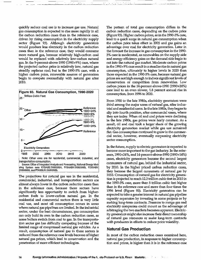
quickly reduce coal use is to increase gas use. Naturalgas consumption is expected to rise more rapidly in allthe carbon reduction cases than in the reference case,driven by rising consumption in the electricity supplysector (Figure 93). Although electricity generatorswould produce less electricity in the carbon reductioncases than in the reference case, they would consumemore natural gas, because relatively high-carbon coalwould be replaced with relatively low-carbon naturalgas. In the 9-percent-above-1990 (1990+9%) case, wherethe projected carbon price is relatively low, natural gassteadily replaces coal; but in the 1990-3% case, with ahigher carbon price, renewable sources of generationbegin to compete successfully with natural gas after2010.
Figure 93. Natural Gas Consumption, 1996-2020
25-Trillion Cubic Feet
20- Other
15-
1 0 -
5 -
Reference1990+24%
——1990+9%~ 1990-3%
1990-3%1990+9%
1990+24%
Reference
Electricity Generators0-r-1995 2000 2005 2010 2015 2020
Note: Other uses are for residential, commercial, industrial, and^transportation consumption.j Source: Office of Integrated Analysis and Forecasting, National Energy Mod-teling System runs KYBASE.D080398A, FD24ABV.D080398B, FD09ABV.D080398B, and FD03BLW.D080398B. j
The projections for natural gas use in the residential,commercial, industrial, and transportation sectors arealmost always lower in the carbon reduction cases thanin the reference case, because those sectors havesignificantly less opportunity to switch from higher-carbon fuels to lower-carbon natural gas. In theresidential and commercial sectors there is very littlecoal use, and most oil consumption occurs in areaswhere natural gas pipelines are limited. In the industrialsector, under the best circumstances, gas consumptioncan only hold its own in the carbon reduction cases, assome boilers switch from coal to gas. In the transporta-tion sector gas has difficulty competing because of thelimited range of compressed natural gas vehicles. As aresult, consumption of natural gas in these sectors isreduced from the reference case levels because of highernatural gas prices, which lead to conservation and thepenetration of more efficient technologies.
The pattern of total gas consumption differs in thecarbon reduction cases, depending on the carbon price(Figure 93). Higher carbon prices, as in the 1990-3% case,lead to a quick surge in natural gas consumption whenthe carbon price takes effect in 2005 and gas gains anadvantage over coal for electricity generation. Later inthe forecast the increase in gas consumption in the 1990-3% case is moderated, as renewables on the supply sideand energy efficiency gains on the demand side begin tocut into the natural gas market. Moderate carbon pricesin the 1990+9% case result in a steadier rise in natural gasconsumption, ultimately to higher levels in 2020 thanthose expected in the 1990-3% case, because natural gasprices are not high enough to induce significant levels ofconservation or competition from renewables. Lowcarbon prices in the 24-percent-above-1990 (1990+24%)case lead to an even slower, 1.8 percent annual rise inconsumption, from 1996 to 2020.
From 1950 to the late 1980s, electricity generators werethird among the major users of natural gas, after indus-trial and residential users. In the late 1980s, they began toslip into fourth position, after commercial users, wherethey are today. When oil and coal prices were decliningin the late 1980s, gas prices were fairly constant. As aresult, oil and coal took a larger share of the growingelectricity generation market while gas use remainedflat. Gas consumption continued to grow in the commer-cial sector, however, eventually surpassing electricitysector consumption.
In the future, supply to electric generators is expected tobecome more important to the gas industry. In the refer-ence, 1990+24%, and 14-percent-above-1990 (1990+14%)cases, electricity generators become the second largestconsumers of natural gas, behind the industrial sector,by 2010. In the higher priced carbon reduction cases,they become the largest consumers of natural gas by2010. Consumption of natural gas for electricity genera-tion is projected to reach 12.2 trillion cubic feet in 2010 inthe 1990-3% case, more than 5 trillion cubic feet higherthan in the reference case and more than four times the1996 level (Figure 93). Electricity generators can beexpected to take a greater interest in natural gas pipelinecapacity expansion by investing in some projects or bymaking long-term contracts. Pressure to merge gas andelectricity companies could mount as the advantage ofarbitraging the two markets becomes apparent. Electric-ity generators might also increase their direct ownershipof natural gas resources or make long-term contractswith producers in efforts to reduce price volatility.
Natural Gas ProductionIn most of the carbon reduction cases examined here,natural gas production, in response to higher consump-tion and prices, is higher than it is in the reference case
96 Energy Information Administration / Impacts of the K. oto Protocol on U.S. Enere Markets;
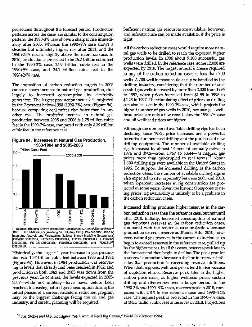
projections throughout the forecast period. Productionpatterns across the cases are similar to the consumptionpattern: the 1990-3% case shows a sharper rise immedi-ately after 2005, whereas the 1990+9% case shows asteadier but ultimately higher rise after 2011, and the1990+24% case is slightly above the reference case. In2010, production is projected to be 26.2 trillion cubic feetin the 1990-3% case, 25.9 trillion cubic feet in the1990+9% case, and 24.1 trillion cubic feet in the
1990+24% case,
The imposition of carbon reduction targets in 2005causes a sharp increase in natural gas production, duelargely to increased consumption by electricitygenerators. The largest production increase is projectedin the 7-percent-below-1990 (1990-7%) case (Figure 94),because competing coal prices rise faster than in anyother case. The projected increase in natural gasproduction between 2005 and 2006 is 1.75 trillion cubicfeet in the 1990-7% case, compared with only 0.39 trillioncubic feet in the reference case.
Figure 94. Increases in Natural Gas Production,1983-1984 and 2005-2006
2 . 0 -
1.5-
1.0-
Trillion Cubic Feet
2005-2006-
0.5-
Sources: History: Energy Information Administration, Annual Energy Review1997, DOE/EIA-0384(97) (Washington, DC, July 1998). Projections: Office ofIntegrated Analysis and Forecasting, National Energy Modeling System runsWBASE.D080398A, FD24ABV.D080398B, FD1998.D080398B, FD09ABVJP080398B, FD1990.D080398B, FD03BLW.D080398B, and FD07BLWJD08039SB. I
Historically, the largest 1-year increase in gas produc-tion was 1.37 trillion cubic feet between 1983 and 1984(Figure 94). However, in 1984 production was recover-ing to levels that already had been reached in 1982, andproduction in both 1983 and 1985 was down from theprevious year. In contrast, the levels expected in 2005-2007—while not unlikely—have never before beenreached. Increasing natural gas consumption during theinitial phases of a carbon emissions reduction programmay be the biggest challenge facing the oil and gasindustry, and careful planning will be required.
Sufficient natural gas resources are available, however,and infrastructure can be made available, if the price isright.
All the carbon reduction cases would require more natu-ral gas wells to be drilled to reach the expected higherproduction levels. In 1996 about 9,100 successful gaswells were drilled. In the reference case, some 12,000 areexpected by 2010. The largest annual increase requiredin any of the carbon reduction cases is less than 700wells. A 700-well increase could easily be handled by thedrilling industry, considering that the number of suc-cessful gas wells increased by more than 2,000 from 1996to 1997, when prices increased from $1.55 in 1995 to$2.23 in 1997. The stimulating effect of prices on drillingcan also be seen in the 1990-3% case, which projects thehighest number of gas wells in 2010, because gas well-head prices are only a few cents below the 1990-7% caseand oil wellhead prices are higher.
Although the number of available drilling rigs has beendeclining since 1982, price increases are a powerfulincentive for increased drilling and the purchase of newdrilling equipment. The number of available drillingrigs increased by almost 14 percent annually between1974 and 1982—from 1,767 to 5,644^-as natural gasprices more than quadrupled in real terms.71 About1,600 drilling rigs were available in the United States in1996. To support the increased drilling in the carbonreduction cases, the number of available drilling rigs isalso expected to rise, especially between 2005 and 2010,when 2-percent increases in rig construction are pro-jected in some years. Given the historical response to ris-ing prices, rig availability is unlikely to be a problem inthe carbon reduction cases.
Increased drilling produces higher reserves in the car-bon reduction cases than the reference case, but not untilafter 2010. Initially, increased consumption of naturalgas depresses reserves in the carbon reduction cases,compared with the reference case projection, becauseproduction exceeds reserve additions. After 2010, how-ever, natural gas reserves in the carbon reduction casesbegin to exceed reserves in the reference case, pulled upby the higher prices. In all the cases, reserves peak late inthe forecast and then begin to decline. The peak year forreserves is important, because a decline in reserves indi-cates that production is exceeding reserve additions.When that happens, wellhead prices tend to rise becauseof depletion effects. Reserves peak later in the highercarbon price cases, as higher wellhead prices sustaindrilling and discoveries over a longer period. In the1990-3% and 1990+9% cases, reserves peak in 2018, com-pared with 2013 in the reference case and 1990+24%case. The highest peak is projected in the 1990-7% case,at 195.5 trillion cubic feet of reserves in 2018. Projections
71T,A. Stokes and M.R. Rodriguez, "44th Annual Reed Rig Census," World Oil (October 1996).

- r • ' ' " " . - •
of reserve levels depend on the assumed levels of natu-ral gas resources and, as such, are highly uncertain, par-ticularly in the offshore regions of the lower 48 States.
In general, increased reserves indicate that a mineralindustry is well prepared to serve its customers;however, reserves must be placed in the context ofproduction to gauge their real adequacy. Reserve-to-production (RP) ratios provide a measure of theadequacy of reserves. In this analysis, RP ratiosgenerally are projected to fall faster in the carbonreduction cases than in the reference case, becauseproduction exceeds replacement of reserves (Figure 95).The path of RP ratios over the forecast is heavilyinfluenced by the production path. When productionincreases steeply in the 1990-3% case the RP ratio dropssteeply, whereas in the 1990+24% case the RP ratio dropsmore steadily to lower ultimate levels. In 1996, the RPratio for natural gas was 8.3. In the reference case, it isprojected to fall to 6.4 in 2020. In the 1990+24% case, theRP ratio in 2020 is slightly lower than in the referencecase and is at the lowest level of any year in the forecast.In the 1990-3% and 1990+9% cases, the RP ratio in 2020exceeds the reference case projection (Figure 95). Thus,when a higher carbon price is projected, the adequacy ofnatural gas reserves improves relative to that projectedin the reference case, because higher gas prices areexpected to lead to more reserve additions.
Most types of natural gas production are projected to behigher in the carbon reduction cases than in thereference case, with the exception of associated-dissolved (AD) and Alaskan gas. AD gas production is afunction of oil production, which is expected to be lowerin the carbon reduction cases than in the referencecase (see the "Oil Production" section below). While
Figure 95. Index of Natural Gas Reserve-to-i Production Ratios, 1990-2020
11.0-Index, 1990=1.0
0.9-
0.8-
0.7-
n R -History Projections
1990-3%Reference1990+9%1990+24%
| 1990 1995 2000 2005 2010 2015 2020I Sources: History: Energy Information Administration, U.S. Crude Oil, NaturalGas, and Natural Gas Liquids Reserves 1996, DOE/EIA-0216(96) (Washington]DC, November 1997), and preceding reports. Projections: Office of IntegratedAnalysis and Forecasting, National Energy Modeling System runs KYBASEJD080398A, FD24ABV.D080398B, FD09ABV.D080398B, and FD03BLWJD080398B. I
increasing in all cases, Alaska's production of naturalgas is expected to be lower in the carbon reduction cases,because the market for Alaskan gas is limited mostly tothe State. Electricity generators in Alaska are alreadymore heavily dependent on natural gas than coal, andtheir opportunities to switch from coal to gas are limited.So, electricity generators reduce gas consumption.Although not included in this analysis, the market forAlaskan natural gas could grow through increasedexportation of liquefied natural gas, manufacturing ofliquids from natural gas (the Fischer-Tropsch process),increased industrial manufacturing, or methanolmanufacturing.
Employment in the oil and gas industries generally hasfallen in recent years, as oil production has declined andproductivity has increased. According to the U.S.Bureau of Labor Statistics, employment in the oil andgas extraction industries declined from 400,000 employ-ees in 1988 to 322,000 in 1996, a reduction of approxi-mately 20 percent. Over the same period, total oil andgas production dropped from 34.9 quadrillion Btu to33.0 quadrillion Btu, a reduction of only 5 percent. Ris-ing productivity accelerated the decline in employmentrelative to the decline in production.
In the reference case, higher natural gas production isprojected to more than offset lower oil production, lead-ing to a total oil and gas production level of 38.6 quadril-lion per year Btu by 2020. Although employment in theoil and gas industries is not included in the projectionsfor this analysis, it is reasonable to expect that theincrease in production would at least reduce the rate ofdecline in employment. In the 1990+9% case, total oiland gas production in 2020 is projected to be 2.1 quadril-lion Btu (about 5 percent) higher than in the referencecase, despite a reduction of 0.5 quadrillion Btu in oil pro-duction. Thus, the projection for the 1990+9% caseimplies that there would be more workers in the naturalgas industry in 2020.
The patterns of U.S. natural gas production projected inthe carbon reduction cases differ among the six onshoreand three offshore producing regions, depending onconsumption and available resources. In the largestproducing regions, the Rocky Mountain and Gulf Coastonshore and Gulf Coast offshore, production risesthroughout the forecast in the reference case, becausesignificant amounts of resources are located in thoseregions, and technology improvements make more ofthe resources available for production in the projectionperiod—particularly, unconventional resources andconventional resources at depths greater than 10,000feet. In the three medium-sized onshore regions,production peaks during the forecast in the referencecase and declines as production becomes more costly. Inthe two least productive regions, the West Coast andPacific offshore, production generally falls throughout
Natural Gas Supply IssuesUncertainty regarding estimates of the Nation's naturalgas resources has always been an issue in projecting pro-duction. Although this study relies on resource estimatesmade by the U.S. Geological Survey (USGS) and MineralsManagement Service (MMS), some uncertainty sur-rounds those estimates. Although many analysts believethat the USGS estimates are too high, an April 1998 studyby the Gas Research Institute (GRI)a contends that theindustry has "significantly underestimated" the growthpotential of existing fields and should look to the Mtdcon-tinent, onshore Gulf Coast, East Texas, and San Juan Basinfor reserve growth. GRI has increased its reserve esti-mates for those areas but maintains that assessing theactual amounts remains a difficult task. Uncertainty is aparticular problem in the offshore area (which the indus-try hopes will provide significant supplies) because notmuch historical data is available for offshore production.Not all of the industry's original hopes may be realized,however. For example, the sub-salt area, which untilrecently was regarded as a promising supply source, is nolonger considered to be as promising.
Another concern about supply availability is access topublic land for drilling. Drilling moratoria have placedoffshore areas in the eastern Gulf of Mexico, North Caro-lina, and California off limits, and drilling is limited insome areas of the West because of concern about emis-sions. Substantial resources in the Arctic National Wild-life Refuge (ANWR)b are also restricted from drilling,although the current inability to market natural gas fromnorthern Alaska renders the accessibility issue moot.
In addition to concerns about supply availability, there iswidespread speculation in the industry as to whether thelevel of production that would be needed to meet thehefty increases in demand projected in various carbonreduction scenarios could be achieved, given currentworldwide shortages of offshore rigs and skilled person-nel. Virtually every available offshore rig was in usethroughout 1997, and capacity expansion has been lim-ited by uncertainty surrounding the actual demand fornew rigs. The lead time for construction of new rigs is 2 to3 years, and costs range from $115 million for a 350-foot
jack up to $325 million for a deepwater semisubmersible.c
Considerable training is needed to develop a workforce,and many people are reluctant to enter the workforcebecause of its cyclical history and their consequent fear offuture layoffs. In addition, there are concerns about theadequacy of the infrastructure to move gas from offshoredrilling platforms to the shore.
To address these uncertainties, several studies are beingundertaken. For example, former Secretary of EnergyFederico Pena commissioned the National PetroleumCouncil (NPC) to undertake a study of whether the indus-try will be able to respond to meet projected demands,and the Natural Gas Supply Association (NGSA) is work-ing on a report that will analyze whether the industry canmeet increased demand projections without increasingwellhead prices.6
Royalty issues are also of concern. The Assistant Secretaryof the Interior for Land and Minerals Management, Rob-ert L. Armstrong, raised the issue of a possible increase inthe deepwater royalty rate to 16.67 percent from 12.5 per-cent after the current "royalty holiday." Although theproposal has not been supported by Congress, the uncer-tainty about royalty relief that stems from any talk aboutchanges could place a damper on investment.
Despite the above concerns, considerable investment isbeing made in the industry. According to Arthur Ander-sen's 10th annual "U.S. Oil & Gas Industry Outlook Sur-vey," executives of mostU.S. exploration-and-productioncompanies plan to increase spending in 1998.f As anexample, Shell has recently announced plans to spendnearly $1 billion to develop three oil-and-gas fields in thedeepwater Gulf of Mexico.6
Clearly, there are conflicting opinions throughout indus-try as to whether steep increases in production can beachieved in a timely fashion, even with significantincreases in wellhead prices. In order for this to happen,the industry first needs to be confident that the demandwill be there, so that the necessary investments in infra-structure, rigs, drilling, and manpower development canbe made in time.
Assessment and Characterization ofLower-48 Oil and Gas Reserve Growth, prepared by Energy and Environmental Analysis, Inc. forthe Gas Research Institute (Chicago, IL, April 1998).
ANWR resources are not included in this analysis.c"Simmons: Offshore Rig Shortage Looms," Oil and Gas Journal (April 27,1998), p. 24.d,,Producers Question Studies Showing Rising Gas Demand But Flat Prices," Inside F.E.R.C.'s Gas Market Report (May 15,1998), p. 2.e"Concerned About Prices, NGSA To Throw Shadow Over Rosy Supply Pictures," Inside F.E.R.C (May 11,1998), p. 7.
E&P Companies Plan To Boost Spending Despite Variety of Concerns—Study," Inside F.E.R.C.'s Gas Market Report (December 26,1997), p. 9.
8"Shell To Spend $1 Billion To Develop Three Gulf Deep-Water Discoveries," InsideF.E.R.C.'s Gas Market Report (April 3,1998), p. 9.
I,,
the forecast, as a small resource base precludes signifi-cant responses to higher prices. Regional production inthe carbon reduction cases is generally higher than in thereference case because prices are higher. In regionswhere production peaks during the forecast, productiontends to peak sooner in the carbon reduction cases,because more gas is produced earlier.
Natural Gas ImportsNatural gas imports are projected to be higher in all thecarbon reduction cases than in the reference case, as theindustry works to meet rising demands for natural gas.In 2010, net natural gas imports are projected to be 4.7trillion cubic feet in the reference case and up to 5.7 tril-lion cubic feet in the carbon reduction cases. Net imports
Energy Information Administration / Impacts of the Kyoto Protocol on U.S. Energy Markets and Economic Activity 99

are highest in the cases with high carbon prices, whereimports surge as the carbon prices are imposed andremain at higher levels than those projected in the refer-ence case. However, by the end of the forecast, the high-est levels of net imports are expected in the 1990-3%case, rather than the 1990-7% case, because consumptionis projected to be higher in the 1990-3% case.
In most of the carbon reduction cases, the majority of thehigher imports come from Canada in 2010, but in the1990-7% and 1990-3% cases at least half of the increasecomes from Mexico. Even though Canada would be sub-ject to its own carbon restrictions, it has a large enoughresource base to increase both domestic consumptionand exports. The Canadian Gas Potential Committeeestimated in 1997 that the Western Canada SedimentaryBasin contained 263 trillion cubic feet of marketablegas.72 In 2010 Natural Resources Canada projects Cana-dian natural gas consumption at 3.6 trillion cubic feet,up 600 billion cubic feet from 1995.73 If carbon reductiontargets were imposed, Canada's gas consumptionwould likely be higher. For example, if gas consumptionin Canada were 10 percent higher in 2010 as a result ofcarbon restrictions, as projected for the United States inthe most stringent carbon reduction cases, it wouldreach 4.2 trillion cubic feet in 2010. Even at that level,however, U.S. prices are expected to be high enough tocontinue the flow of imports from Canada.
In the carbon reduction cases, Mexico is a net exporter ofnatural gas to the United States in 2010, whereas it is anet importer in the reference case. Mexico begins toexport gas to the United States in the carbon reductioncases in response to higher consumption and higherwellhead prices. Net imports of liquefied natural gas(LNG) reach one-third of a trillion cubic feet annually inall the carbon reduction cases but do so more quickly inthe cases with higher projected carbon prices.
Natural Gas PipelinesInterstate natural gas pipeline capacity additions wouldneed to be higher in the carbon reduction cases than theyare in the reference case projections, but they areexpected to be manageable. In the reference case, cumu-lative additional natural gas pipeline capacity crossingthe 12 regions used for this analysis are projected toincrease to 52.5 trillion cubic feet of design capacity in2010 from the 1996 capacity of 43.0 trillion cubic feet. Themost significant increase is projected from 1998 to 2001,when capacity increases by 6.3 trillion cubic feet becauseof increasing consumption in the Midwest and North-east not because of carbon reduction policies. Duringthe 1998-2001 period, the Alliance pipeline is expectedto come down to the Midwest from Canada, andthe Maritimes/Northeast and Portland Natural Gas
Transmission System pipelines are expected to comedown from Sable Island in Canada to the northeasternUnited States. After 2001, pipeline capacity is projectedto increase more gradually through 2010.
In the carbon reduction cases, the largest 1-year increasein pipeline capacity after 2001 is seen from 2011 to 2012in the 1990+9% and 1990+14% cases, when capacityincreases by 1.6 trillion cubic feet. The capacity increasesin this period are primarily out of Texas, Louisiana, andOklahoma, through the South, to the southern coastalStates in response to growing consumption. The largestincrease soon after imposition of the carbon price is from2006 to 2007 in the 1990-3% case, when capacity is pro-jected to increase by 1.4 trillion cubic feet. The increase ismainly from west to east, from the Texas-Oklahoma-Louisiana region to the Middle South.
Historically, the largest recent annual increase in pipe-line capacity was 1.6 trillion cubic feet from 1991 to 1992,partly because of the construction of four major pipe-lines into California from the Mountain States (KernRiver, Mohave, El Paso, and Transwestern) and twomajor pipelines out of Canada (Great Lakes into theMidwest and Iroquois into the New York/New Englandarea). In view of the historical and expected near-termincreases in capacity, capacity expansion is not likely tobe a problem in any carbon reduction scenario, as longas pipeline requirements are known 2 to 3 years inadvance.
Natural Gas PricesNatural gas prices are higher in the carbon reductioncases than in the reference case, both at the wellhead andat the burner tip. At the wellhead, higher production tosatisfy increased natural gas consumption, in the face ofincreasingly expensive resources, boosts prices. At theburner tip, adding carbon prices to resource costs couldmore than double some end-use prices.
In the reference case, lower 48 wellhead natural gasprices are projected to rise from $2.24 per thousand cubicfeet in 1996 to $2.33 in 2010 in 1996 dollars (Figure 96).The 2010 wellhead prices are more than 40 cents perthousand cubic feet or 19 and 29 percent higher in the1990-3% and 1990+9% cases, which project higherconsumption and the use of increasingly expensiveresources. The highest wellhead prices in 2010 are seenin the 1990-7% case at $3.03 per thousand cubic feet,where carbon prices are highest in 2010.
The pattern of natural gas wellhead prices is similar tothe consumption and production patterns (see above).In the reference case, prices rise gradually, but in thecarbon reduction cases prices rise quickly after a carbon
^Canadian Gas Potential Committee, Natural Gas Potential in Canada (Calgary: University of Calgary, 1997), Figure 1.2.73Calculated from Natural Resources Canada, Canada's Energy Outlook 1996-2020 (Ottawa: Natural Resources Canada, 1997), Annex C.

price is imposed in 2005. In the cases with higher pro-jected carbon prices, gas prices rise more quickly, thenflatten out as energy conservation on the demand sideand renewable energy production on the supply side
slow the overall rate of growth in natural gas con-sumption. When moderate carbon prices are projected,gas prices rise more steadily but ultimately reach higherlevels.
Natural Gas Pipeline ExpansionThere are three ways of increasing pipeline capacity. Thesimplest and least expensive is to increase throughput byincreasing compression at compressor stations. The sec-ond is through a process called "looping," in which paral-lel pipe is laid next to existing pipe to increase capacityalong an existing route. The third, and most costly, is tobuild new pipe, usually entailing additional costs for landand/or right-of-way.
Two key criteria must be met in order for an expansionproject even to be proposed: (1) the existence of demandmust be shown, and (2) the project must be proven to befinancially viable. Four steps are needed to bring a projectto fruition: (1) an open season of 1 to 2 months duringwhich bids for the proposed capacity are solicited andreceived, (2) a planning stage of 3 to 5 months, (3) filingwith the Federal Energy Regulatory Commission (FERC)for approval, with an average time of 15 months (rangingfrom 5 to 18 months), and (4) an actual construction stage,which averages 6 to 9 months. Barring unforeseen delays,capacity can be added with a lead time of 2 to 3 years.Problems that can slow down the process include the fil-ing of environmental impact statements and acquiringnecessary approvals, and changes in market conditions(such as the changing market conditions that affected theAltamont project, which was approved in 1990 but stillhas not been constructed). FERC has seen a significantincrease recently in the number of comments and protestsreceived on proposed expansion projects. Another poten-tial problem is competition between two pipelines forexpansion to serve the same market, such as the recentcompetition to move supplies from Western Alberta,Canada, into the Midwest.
Greater increases in pipeline capacity than those pro-jected in the carbon reduction cases are likely betweennow and 2000. More than 116 expansion projects havealready been proposed. For the 71 projects for which pre-liminary estimates are available, the estimated total costsexceed $11 billion. In 2000 alone, $4.6 billion in expendi-tures is anticipated, as several major projects maybe com-pleted.8 The added capacity is needed to provide access tonew and expanding production areas, such as Canadaand the deep offshore, and to accommodate shifts indemand patterns, such as new demands for natural gas toreplace electricity generation capacity lost as a result ofnuclear retirements.
Although there is speculation within the industry as towhether the needed expansions can occur, two factorssupport an optimistic outlook. The first is changes inFERC policy, which now leans more toward letting thepipelines assume more risk rather than requiring firmcontracts to be in place before approving an expansion.
This may work to speed up the approval process. The sec-ond is projected increases in natural gas demand, inde-pendent of the Kyoto Protocol. Demand growth is alreadyanticipated to result from electric utility restructuringactivities in a growing number of States, retirements ofnuclear facilities, and measures included in the Presi-dent's Climate Change Technology Initiative (a $6.3 bil-lion initiative), which will proceed regardless of the fateof the Kyoto Protocol. If the anticipated increases indemand do materialize, they could provide the impetusfor much of the capacity increase that would be needed inthe event that the Kyoto Protocol is ratified.
On the other hand, financial considerations are creatingsome uncertainty about the responsiveness of the pipe-line industry. A major issue is whether the economic cli-mate for investment will continue to be favorable.Pipeline owners are claiming that they currently face con-siderable risk because of increased competition and thethreat of capacity turnback. While the Natural Gas SupplyAssociation (NGSA) contends that the FERC's currentpolicy for determining pipeline returns on equity is fairand properly accounts for the risk faced by the pipelineindustry, the Interstate Natural Gas Association of Amer-ica (INGAA) contends that the Commission's genericmethod artificially lowers allowed returns, and that ratesshould be calculated on a case-by-case basis. Pipelineexecutives contend that the 12- to 13-percent average rateof return for pipelines in 1996 was far lower than the 20-percent rate earned by most public companies. Inresponse to the industry's concerns, the FERC is currentlyevaluating possible changes in the method used to calcu-late pipeline returns. As even more risk is associated withthe levels of expansion forecast in the carbon reductioncases, a key question is, "Who will assume the addedrisk—utilities that need the gas, other consumers willingto contract for gas, or the pipeline companies?"
Despite the obvious uncertainties, recent history showsthat the industry can handle expansions of the same orderof magnitude as those being projected as a result of theKyoto Protocol. Changes in the pipeline industry betweennow and the time of the rapid capacity expansions thatare expected to be needed to support electricity suppliersafter the enactment of carbon reduction targets will be keyto the industry's ability to respond. This is one of theissues that the upcoming NPC study commissioned byformer Secretary of Energy Federico Pena will be address-ing. Several other industry studies are underway toevaluate the industry's ability to respond, including anINGAA study that "will be looking at what needs to bedone for the pipeline industry" to achieve a market of 30trillion cubic feet by 2010.°
aEnergy Information Administration, Office of Oil and Gas, EIAGIS Natural Gas Geographic Information System Natural Gas ProposedConstruction Database (Washington, DC, preliminary as of April 1998).
b"NGSA: Return-on-Equiry Fair Despite Protests by Pipelines," Natural Gas Week (March 9,1998), p. 6.
formation Administration l\n . acts of the K oto Protocol on U.S. Ene. Markets and Economic ActivJ. 101

Figure 96. Natural Gas Wellhead Prices, 1970-2020 {1996 Dollars per Thousand Cubic Feet
1990+9%1990-3%
1990+24%
Reference
Figure 97. Delivered Natural Gas Prices in theResidential Sector, 1970-2020
1996 Dollars per Thousand Cubic Feet
1990 2000 2010 2020Sources: History: Energy Information Administration, Annual Energy Review
\I997, DOE/EIA-0384(97) (Washington, DC, July 1998). Projections: Office ofIntegrated Analysis and Forecasting, National Energy Modeling System runskYBASE.D080398A, FD24ABV.D080398B, FD09ABV.D080398B, andFD03BLW.D080398B. i
On a regional basis, access to end-use markets heavilyinfluences wellhead prices. Some of the lowest wellheadprices are seen in the Rocky Mountain region, whereaccess to eastern markets is limited by pipelineconstraints. This is balanced by wellhead prices in thetwo largest producing regions in this study, the GulfCoast onshore and offshore, which have prices slightlyabove the national average in 1996. Wellhead prices arecurrently higher in the Northeast region than any other,where demand is significant and growing. Regionalprices are generally higher in the carbon reduction cases,because of higher demand. Though more exaggerated,the pattern of growth across regions is much the same asin the reference case.
The projected end-use prices for natural gas in thecarbon reduction cases are double the prices in thereference case at their peak in the most extreme cases.The main components of end-use prices are thewellhead price, the carbon price, and transmission anddistribution margins. On a percentage basis, residentialprices are the least affected by the imposition of carbonprices, and the prices to electricity generators are themost affected (the projected carbon price is almost thesame for both sectors, but gas prices are significantlyhigher in the residential sector). In 1996, natural gasprices for end users in the residential sector, which hasthe largest number of end-use customers, were $6.37 perthousand cubic feet. In the 1990-3% case, residentialprices are expected to peak in 2013 at $11.31 perthousand cubic feet (in 1996 dollars), compared with$5.71 in the reference case (Figure 97). The difference isalmost entirely attributable to the carbon price, whichadds $4.20 to residential gas prices in 2013. Wellheadprices and transmission margins are also projected to behigher, however, because of higher in total gasconsumption even though residential consumption is
1990-7%1 S3 0-3%19901990+9%1990+14%1990+24%
Reference
1970 1980 1990 2000 2010 2020Sources: History: Energy Information Administration, Annual Energy Review,
\1997, DOE/EIA-0384(97) (Washington, DC, July 1998). Projections: Office oiIntegrated Analysis and Forecasting, National Energy Modeling System runsKYBASE.D080398A, FD24ABV.D080398B, FD1998.D080398B, FD09ABV,'D080398B, FD1990.D080398B, FD03BLW.D080398B, and FD07BLW.D08Q398B.
lower. In the residential sector, margins for distributionservices are higher because fixed costs must be spreadover a smaller consumption base. In the 1990-7% case,residential prices are projected to peak at $12.10 perthousand cubic feet in 2013, because this case has thehighest carbon prices. End-use prices in the carbonreduction cases follow a pattern similar to the pattern ofcarbon prices.
The story is much the same for the electricity supplysector, where the most growth in consumption isexpected, except that the projected difference betweenwellhead and end-use margins is much smaller (lessthan 10 cents per thousand cubic feet) in the 1990-3%case in 2010. The differences in margins is not as high asin the residential sector because higher electric generatorconsumption allows gas utilities to spread their fixedcosts over a larger volume of gas. In 1996, deliveredprices to electricity generators were $2.70 per thousandcubic feet. At their peak in 2014, prices in the 1990-3%case are projected to be $8.27 per thousand cubic feet,compared with $3.05 in the reference case. As in theresidential sector, the higher the carbon price, the higherthe end-use price.
End-use prices for natural gas are affected by their dis-tance from the sources of supply. End-use prices in theTexas-Louisiana region are currently less than half ofprices in New England, for example. Although NewEngland currently has the highest average natural gasend-use prices, prices are expected to be highest in theMid-Atlantic region in a few years, as new pipeline proj-ects are completed into New England and as consump-tion for electric generation increases. Regional prices aregenerally higher in the carbon reduction cases than in
the reference case, because of higher demand. Theyshow much the same pattern of growth as in the refer-ence case.
Oil Industry
Oil is a larger source of energy than natural gas. Nearly40 percent of U.S. energy comes from oil, most of whichis used to fuel our vehicles and industry. Gasoline anddiesel oil fuel more than 200 million vehicles, one forevery 1.3 people in the country. Almost half of our oilwas imported by tanker ship from Venezuela, Mexico,Saudi Arabia, and other countries at a cost of more than$60 billion in 1996. The rest is produced domestically,mainly in Texas, Alaska, Louisiana, and California, andshipped by pipeline and tanker. With the exception ofresidual fuel oil, this easily moved, universally-availableliquid tends to cost more per Btu than other forms ofenergy.
In 1996, oil combustion produced 621 million metrictons of carbon emissions in the United States, over two-fifths of the total and more than those produced fromburning coal. The transportation sector was responsiblefor the major share of those emissions, almost threequarters, followed by industrial and residential emis-sions in order of magnitude. In 2010, if no carbon reduc-tion measures are put in place, emissions from oilcombustion are expected to be more than 130 millionmetric tons higher man they were in 1996, although theirshare of the total will be slightly lower.
U,S. oil consumption is expected to increase between1996 and 2010 in the reference case, despite a projecteddecline in domestic oil production. Most of the growth isexpected in the transportation sector, where oil con-sumption is projected to increase by almost 30 percentfrom 1996 to 2010. About half the increase comes fromlight-duty vehicle travel and more than 20 percent fromincreased air travel. Oil use in the industrial sector isprojected to increase by about 15 percent between 1996and 2010, with more than three-fifths of the increasecoming in refining and petrochemical feedstocks. As aresult of these increases, oil's share of the energy marketwill increase slightly over time.
While petroleum production from conventional sourcesin the lower 48 States and in Alaska is expected to fallbetween 1996 and 2010, enhanced oil recovery and off-shore production are expected to increase, but notenough to prevent an overall decline. Net imports ofcrude oil and petroleum products are projected to rise tofill the gap between consumption and production. In thereference case, almost three-fifths of the U.S. oil supplyin 2010 is projected to come from imports, with aboutthree-fourths of total imports entering the country in theform of crude oil and the rest as finished or unfinished
products. Gross refinery margins are projected toincrease on the strength of increased refinery through-put and capacity expansion. End-use prices show littlechange in the reference case, as increases in world oilprices are balanced by assumed reductions in motor fueltaxes. Federal taxes on gasoline and diesel fuel areassumed to stay constant in real dollar terms, whichwould mean a decline in nominal terms.
Policies aimed at reducing carbon emissions would leadto lower consumption, production, imports, and refin-ery margins for the U.S. oil industry. On the other hand,end-use prices and market share would be higher.Higher end-use prices—reflecting new carbon prices—would reduce consumption in the carbon reductioncases, lessening the need for domestic production andforeign imports. Refinery margins in those cases wouldbe lower, because consumption of petroleum productsand expansion of refinery capacity are projected to belower than in the reference case. Despite the lower levelsof oil consumption projected in the carbon reductioncases, oil's share of the energy market would be higheras a result of an even larger drop in coal use. Forexample, in the 1990-3% case, oil is projected to claim 41percent of the domestic energy market in 2010 and coaljust 7 percent, as compared with their respective 38-percent and 22-percent shares in 1996.
Oil ConsumptionOil consumption is expected to be lower in the carbonreduction cases than in the reference case (Figure 98),with most of the difference in the transportation sector.Current petroleum product consumption is at about theprevious peak level of consumption reached 20 yearsago. In the reference case, consumption rises from 18.5million barrels per day in 1996 to 22.5 million barrels perday in 2010. In title carbon reduction cases, higher carbonprices overwhelm lower crude oil prices and lead tolower levels of oil consumption in 2010—22.0 millionbarrels per day in the 1990+24% case and 20.0 millionbarrels per day in the 1990-3% case. Consumption in thetransportation sector is particularly affected. More than65 percent of the difference between the reference andthe carbon reduction cases in 2010 is in the trans-portation sector.
In the reference case, petroleum consumption risesthroughout the forecast. Consumption also rises con-tinually throughout the forecast in the carbon reductioncase with the lowest projected carbon prices, the1990+24% case. In the other cases, consumption declinesduring the 2005-2009 period after the carbon price isimposed. The higher the carbon price, the greater thedecline in consumption. After 2009, consumption risesin all cases through the rest of the forecast, because high-way and air travel increase while carbon prices changemodestly.
Energy Information Administration / Impacts of the Kyoto Protocol on U.S. Energy Markets and Economic Activity 103

Figure 98. Petroleum Consumption, 1970-2020
25-
20-
'15-
Million Barrels per Day
5 -
History
Reference1990+24%
^ 1 9 9 0 + 9 %
Projections
1970 1980 1990 2000 2010 2020
| Sources: History: Energy Information Administration, Annual Energy Review\1997, DOE/E!A-0384(97) (Washington, DC, July 1998). Projections: Office ofIntegrated Analysis and Forecasting, National Energy Modeling System runs'KYBASE.D080398A, FD24ABV.D080398B, FD09ABV.D080398B, andFD03BLW.D080398B. j
Oil use in the transportation sector is expected to absorbthe largest share of the projected declines between 2005and 2009, accounting for more than 85 percent of thetotal drop in oil consumption in the three most stringentcarbon reduction cases, with smaller reductions in theresidential, commercial, and industrial sectors. In the1990-3% case, transportation consumption falls from14.2 million barrels per day in 2004 to 13.5 millionbarrels per day in 2009, followed by a continuingincrease to 15.0 million barrels per day in 2020. Duringthe period of declining consumption, high carbon pricesproduce rapid increases in transportation fuel prices.After 2009, when consumption begins to rise, fuel pricesin the transportation sector are generally level ordeclining, as the carbon prices decline.
Oil Production
U.S. oil production declines steadily throughout theforecast both in the reference case and in the carbonreduction cases, but lower consumption and diminish-ing oil reserves in the later years of the carbon reductioncases lead to larger production declines. In the referencecase, crude oil production is projected to drop from 6.5million barrels per day in 1996 to 5.9 million barrels perday in 2010, compared with 5.8 million barrels per day inthe 1990+24% case and 5.7 million barrels in the1990+9% and 1990-3% cases in 2010. The higher the car-bon price, the lower is the crude oil price, the less is thebuildup in reserves, and the lower is oil production,because the higher carbon prices overwhelm lowercrude oil prices.
Domestic oil drilling activity rises steadily in the refer-ence case and in the least stringent carbon reductioncase. In the more stringent cases, drilling generallyincreases, but declines are projected in the middle years
Figure 99. Lower 48 Crude Oil Reserve Additions,1990-2020
I Billion Barrels2 .5-
2.0-
1.5-
1.0-
|0.5-
History
! 0-r-
Reference1990+24%1990+9%
Projections
i 1990 1995 2000 2005 2010 2015 2020 j
j Sources: History: Energy Information Administration, U.S. Crude Oil, Natural[Gas, and Natural Gas Liquids Reserves 1996, DOE/EIA-0216(96) (Washington]DC, November 1997), and preceding reports. Projections: Office of Integrated;Analysis and Forecasting, National Energy Modeling System runs KYBASEiD080398A, FD24ABV.D080398B, FD09ABV.D080398B, and FD03BLWD080398B. J
of the forecasts, when high carbon prices depress oilprices. The lowest levels of drilling activity are seen inthe cases with the highest projected carbon prices, whichresult in the lowest wellhead prices.
Despite the projections of increased oil drilling both inthe reference case and in the carbon reduction cases, oilreserves are not expected to rise over the forecast period.Declining reserves are projected in all the cases, becausereserve additions do not exceed production. For exam-ple, all the carbon reduction cases show reserve addi-tions of only 1.9 billion barrels in 2005 (Figure 99), whenproduction is projected to be about 2.2 billion barrels forthe year. Thus, oil reserves decline. In the reference case,higher oil prices sustain enough drilling for annualreserve additions to peak at 2.0 billion barrels in 2009. Inthe more stringent carbon reduction cases, however,declining oil prices cause reserve additions to fall after2005. The inability of the oil industry to replace reserveshas less effect on oil prices than the inability to replacegas reserves has on gas prices, because oil prices are setin a world market, and because the RP ratios for oil areactually projected to rise.
Oil RP ratios, which are indicative of the industry's abil-ity to sustain production, rise over the forecast both inthe reference case and in the carbon reduction cases, asoil production falls more quickly than reserves. The RPratio in the reference case rises from 7.1 in 1996 to 7.3 in2010. RP ratios in the carbon reduction cases are slightlylower, because the low oil prices in the carbon reductioncases depress reserve additions more than production.
Most types of oil production are projected to be lower inthe carbon reduction cases than in the reference case,
104 Enerav Information Administration / Imnants nf tho tCvntn Pm»nr>ni nn 11 c cno C—__-:- A-H..U..

and most of the lower production in the carbon reduc-tion cases is in lower 48 onshore conventional andenhanced oil recovery production—the two types ofproduction that are the most responsive to lower oilprices. In 2010, conventional onshore lower 48 oil pro-duction is 90,000 barrels per day lower in the 1990-3%case than in the reference case, 60,000 barrels per daylower in the 1990+9% case, and 20,000 barrels per daylower in the 1990+24% case. Enhanced oil recovery is50,000 barrels per day lower in the 1990-3% case, 40,000barrels per day lower in the 1990+9% case, and 10,000barrels per day lower in the 1990+24% case.
Regionally, oil production is generally lower in the car-bon reduction cases than in the reference case. It is sig-nificantly lower in the Southwest (western Texas andeastern New Mexico), in the Rocky Mountains, and inthe offshore Gulf Coast, which are the largest producingregions. In the 1990-3% case, for example, the projectedproduction in 2010 in each of these regions is 40,000 bar-rels per day less than projected in the reference case. Inthe Midcontinent region (Kansas, Oklahoma, andArkansas), oil production is slightly higher in the morestringent carbon reduction cases than in the referencecase, because increased drilling for gas in the carbonreduction cases leads to more oil discoveries and greateroil production; however, the peak difference is onlyabout 10,000 barrels per day.
Regional crude oil prices are most affected by the qualityof the crude oil. West Coast crude oil prices are generallylower than prices in the rest of the Nation because thedensity of West Coast crude oils is higher. Dense crudeoils contain less of the higher-valued light products, likegasoline or diesel fuel, so their value is lower. Crude oilprices are lower in the carbon reduction cases, but therelationships among regional prices is the same as in thereference case.
OH ImportsThe projections for net imports of crude oil andpetroleum products are lower in the carbon reductioncases than in the reference case, because oil consumptionis projected to be lower, with domestic sourcesproviding a greater share of the Nation's oil needs. As ashare of total consumption, net oil imports reach 59percent in 2010 in the reference and 1990+24% cases butonly 54 percent in the 1990-3% case and 56 percent in the1990+9% case. In all the cases, the projected importlevels are above current levels, which are the highest yetrecorded. The total value of net oil imports in 2010 is$103 billion in the reference case but only $96 billion inthe 1990+24% case, $82 billion in the 1990+9% case, and$70 billion in the 1990-3% case (Figure 100). Both valuesare well below the 1980 peak of $138 billion (in 1996dollars). Even in 2020, the total projected expendituresfor oil imports in the reference case are only $123 billion.
Net crude oil imports rise steadily throughout theforecast in the reference case and in the 1990+24% and1990+9% cases. In the 1990 stabilization, 1990-3%, and1990-7% cases, however, net crude oil imports begin tofall when the carbon price is first imposed, bottomingout in 2009 before beginning to rise again. Imposition ofrelatively high carbon prices causes oil consumption—and imports—to fall temporarily in these cases.
Net petroleum product imports are affected morestrongly than crude oil imports in the carbon reductioncases, because imported crude oil is generally morevaluable to U.S. refiners than imported products inas-much as profits are maximized only at high rates ofrefinery utilization. In the reference case, net productimports rise from 1.1 million barrels per day in 1996 to3.1 million barrels per day in 2010. In comparison, thecorresponding increases are only 70,000 barrels per dayin the 1990-3% case, 760,000 barrels per day in the1990+9% case, and 1.64 million barrels per day in the1990+24% case. In the reference case and in the less strin-gent carbon reduction cases, net petroleum productimports exceed the historic 1973 peak of 2.8 million bar-rels per day at some time during the forecast, beginningas early as 2009 in the reference case, for example.
In the two most stringent reduction cases, unlike theother cases, product imports fall from 2004 through 2008because of a decline in petroleum product consumption,and net product imports stay below the historic peakthrough 2020. In the 1990-7% case, net product importsremain below even their 2004 peak of 2 million barrelsper day through 2020.
Figure 100. NetExpenOil and Pel
Billion J996 Dollars140- I
120-
100-
8 0 - i
6 0 - "
4 0 -
2 0 -
n
VJHistory
1980 1990
ditures for Imported Cruderoleum Products, 1974-2020
Projections
2000 2010
^ Reference
1990+24%^ 1 9 9 0 + 1 4 %^ 1 9 9 0 + 9 %
^ 1 9 9 0 - 7 %
2020
Sources: History: Energy Information Administration, Monthly Energy'peview June 1998, DOE/EIA-0035(98/06) (Washington, DC, June 1998^Projections: Office of Integrated Analysis and Forecasting, National EnergyModeling System runs KYBASE.D080398A, FD24ABV.D080398B, FD1998.JD080398B, FD09ABV.D080398B, FD1990.D080398B, FD03BLW.D080398Bjand FD07BLW.D080398B. i
Energy Information Administration / Impacts of the Kyoto Protocol on U.S. Energy Markets and Economic Activity 105
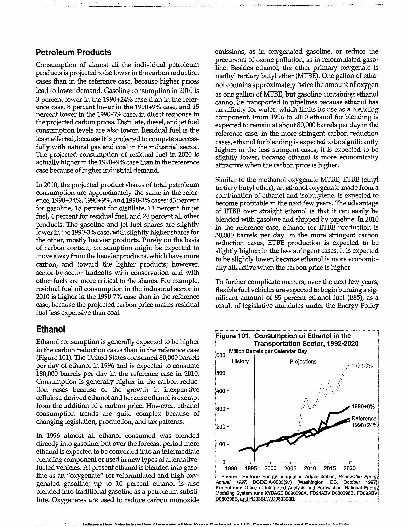
Petroleum ProductsConsumption of almost all the individual petroleumproducts is projected to be lower in the carbon reductioncases than in the reference case, because higher priceslead to lower demand. Gasoline consumption in 2010 is3 percent lower in the 1990+24% case than in the refer-ence case, 8 percent lower in the 1990+9% case, and 15percent lower in the 1990-3% case, in direct response tothe projected carbon prices. Distillate, diesel, and jet fuelconsumption levels are also lower. Residual fuel is theleast affected, because it is projected to compete success-fully with natural gas and coal in the industrial sector.The projected consumption of residual fuel in 2020 isactually higher in the 1990+9% case than in the referencecase because of higher industrial demand.
In 2010, the projected product shares of total petroleumconsumption are approximately the same in the refer-ence, 1990+24%, 1990+9%, and 1990-3% cases: 43 percentfor gasoline, 18 percent for distillate, 11 percent for jetfuel, 4 percent for residual fuel, and 24 percent all otherproducts. The gasoline and jet fuel shares are slightlylower in the 1990-3% case, with slightly higher shares forthe other, mostly heavier products. Purely on the basisof carbon content, consumption might be expected tomove away from the heavier products, which have morecarbon, and toward the lighter products; however,sector-by-sector tradeoffs with conservation and withother fuels are more critical to the shares. For example,residual fuel oil consumption in the industrial sector in2010 is higher in the 1990-7% case than in the referencecase, because the projected carbon price makes residualfuel less expensive than coal.
EthanolEthanol consumption is generally expected to be higherin the carbon reduction cases than in the reference case(Figure 101). The United States consumed 80,000 barrelsper day of ethanol in 1996 and is expected to consume180,000 barrels per day in the reference case in 2010.Consumption is generally higher in the carbon reduc-tion cases because of the growth in inexpensivecellulose-derived ethanol and because ethanol is exemptfrom the addition of a carbon price. However, ethanolconsumption trends are quite complex because ofchanging legislation, production, and tax patterns.
In 1996 almost all ethanol consumed was blendeddirectly into gasoline, but over the forecast period moreethanol is expected to be converted into an intermediateblending component or used in new types of alternative-fueled vehicles. At present ethanol is blended into gaso-line as an "oxygenate" for reformulated and high oxy-genated gasoline; up to 10 percent ethanol is alsoblended into traditional gasoline as a petroleum substi-tute. Oxygenates are used to reduce carbon monoxide
emissions, as in oxygenated gasoline, or reduce theprecursors of ozone pollution, as in reformulated gaso-line. Besides ethanol, the other primary oxygenate ismethyl tertiary butyl ether (MTBE). One gallon of etha-nol contains approximately twice the amount of oxygenas one gallon of MTBE, but gasoline containing ethanolcannot be transported in pipelines because ethanol hasan affinity for water, which limits its use as a blendingcomponent. From 1996 to 2010 ethanol for blending isexpected to remain at about 80,000 barrels per day in thereference case. In the more stringent carbon reductioncases, ethanol for blending is expected to be significantlyhigher; in the less stringent cases, it is expected to beslightly lower, because ethanol is more economicallyattractive when the carbon price is higher.
Similar to the methanol oxygenate MTBE, ETBE (ethyltertiary butyl ether), an ethanol oxygenate made from acombination of ethanol and isobutylene, is expected tobecome profitable in the next few years. The advantageof ETBE over straight ethanol is that it can easily beblended with gasoline and shipped by pipeline. In 2010in the reference case, ethanol for ETBE production is30,000 barrels per day. In the more stringent carbonreduction cases, ETBE production is expected to beslightly higher; in the less stringent cases, it is expectedto be slightly lower, because ethanol is more economic-ally attractive when the carbon price is higher.
To further complicate matters, over the next few years,flexible fuel vehicles are expected to begin burning a sig-nificant amount of 85 percent ethanol fuel (E85), as aresult of legislative mandates under the Energy Policy
Figure 101. Consumption of Ethanol in theTransportation Sector, 1992-2020
600-Million Barrels per Calendar Day
History Projections, 1990-3%
1990+9%
Reference1990+24%i
0-T1990 1995 2000 2005 2010 2015 2020 ]
Sources: History: Energy Information Administration, Renewable Energy'Annual 1997, DOE/EIA-0603(97) (Washington, DC, October 1997)JProjections: Office of Integrated Analysis and Forecasting, National EnergyModeling System runs KYBASE.D080398A, FD24ABV.D080398B, FD09ABVJb080398B.andFD03BLW.D080398B. j
U« IT, . * . * * n—*
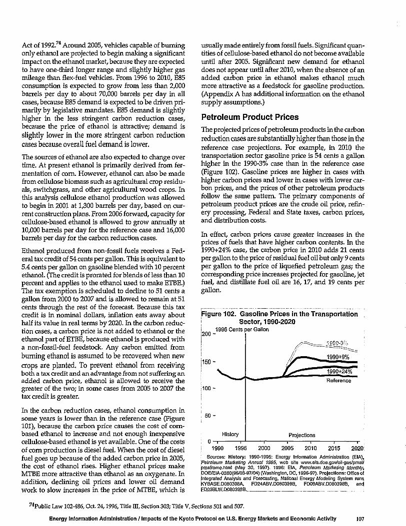
Act of 1992.74 Around 2005, vehicles capable of burningonly ethanol are projected to begin making a significantimpact on the ethanol market, because they are expectedto have one-third longer range and slightly higher gasmileage than flex-fuel vehicles. From 1996 to 2010, E85consumption is expected to grow from less than 2,000barrels per day to about 70,000 barrels per day in allcases, because E85 demand is expected to be driven pri-marily by legislative mandates. E85 demand is slightlyhigher in the less stringent carbon reduction cases,because the price of ethanol is attractive; demand isslightly lower in the more stringent carbon reductioncases because overall fuel demand is lower.
The sources of ethanol are also expected to change overtime. At present ethanol is primarily derived from fer-mentation of corn. However, ethanol can also be madefrom cellulose biomass such as agricultural crop residu-als, switchgrass, and other agricultural wood crops. Inthis analysis cellulose ethanol production was allowedto begin in 2001 at 1,300 barrels per day, based on cur-rent construction plans. From 2006 forward, capacity forcellulose-based ethanol is allowed to grow annually at10,000 barrels per day for the reference case and 16,000barrels per day for the carbon reduction cases.
Ethanol produced from non-fossil fuels receives a Fed-eral tax credit of 54 cents per gallon. This is equivalent to5.4 cents per gallon on gasoline blended with 10 percentethanol. (The credit is prorated for blends of less than 10percent and applies to the ethanol used to make ETBE.)The tax exemption is scheduled to decline to 51 cents agallon from 2000 to 2007 and is allowed to remain at 51cents through the rest of the forecast. Because this taxcredit is in nominal dollars, inflation eats away abouthalf its value in real terms by 2020. In the carbon reduc-tion cases, a carbon price is not added to ethanol or theethanol part of ETBE, because ethanol is produced witha non-fossil-fuel feedstock. Any carbon emitted fromburning ethanol is assumed to be recovered when newcrops are planted. To prevent ethanol from receivingboth a tax credit and an advantage from not suffering anadded carbon price, ethanol is allowed to receive thegreater of the two; in some cases from 2005 to 2007 thetax credit is greater.
In the carbon reduction cases, ethanol consumption insome years is lower than in the reference case (Figure101), because the carbon price causes the cost of corn-based ethanol to increase and not enough inexpensivecellulose-based ethanol is yet available. One of the costsof corn production is diesel fuel. When the cost of dieselfuel goes up because of the added carbon price in 2005,the cost of ethanol rises. Higher ethanol prices makeMTBE more attractive than ethanol as an oxygenate. Inaddition, declining oil prices and lower oil demandwork to slow increases in the price of MTBE, which is
usually made entirely from fossil fuels. Significant quan-tities of cellulose-based ethanol do not become availableuntil after 2005. Significant new demand for ethanoldoes not appear until after 2010, when the absence of anadded carbon price in ethanol makes ethanol muchmore attractive as a feedstock for gasoline production.(Appendix A has additional information on the ethanolsupply assumptions.)
Petroleum Product PricesThe projected prices of petroleum products in the carbonreduction cases are substantially higher than those in thereference case projections. For example, in 2010 thetransportation sector gasoline price is 54 cents a gallonhigher in the 1990-3% case than in the reference case(Figure 102). Gasoline prices are higher in cases withhigher carbon prices and lower in cases with lower car-bon prices, and the prices of other petroleum productsfollow the same pattern. The primary components ofpetroleum product prices are the crude oil price, refin-ery processing, Federal and State taxes, carbon prices,and distribution costs.
In effect, carbon prices cause greater increases in theprices of fuels that have higher carbon contents. In the1990+24% case, the carbon price in 2010 adds 21 centsper gallon to the price of residual fuel oil but only 9 centsper gallon to the price of liquefied petroleum gas; thecorresponding price increases projected for gasoline, jetfuel, and distillate fuel oil are 16,17, and 19 cents pergallon.
Figure 102. Gasoline Prices in the TransportationSector, 1990-2020
200
150
100
50
0
1996 Cents f
_
-
History
• i
)er Gallon
/L ^ 1990+9%
Projections
1990 1995 2000 2005 2010 2015 2020:Sources: History: 1990-1995: Energy Information Administration (EIA),
'Petroleum Marketing Annual 1995, web site www.eia.doe.gov/oil-gas/pmal/pmaframe.html (May 30, 1997). 1996: EIA, Petroleum Marketing Monthly^DOE/EIA-0380(96/03-97/04) (Washington, DC, 1996-97). Projections: Office ofintegrated Analysis and Forecasting, National Energy Modeling System runs,)<YBASE.D080398A, FD24ABV.D080398B, FD09ABV.D080398B, andEDQ3BJ-W.D0a03.9SB. j
74Public Law 102-486, Oct. 24,1996, Title IE, Section 303; Title V, Sections 501 and 507.
Energy Information Administration / Impacts of the Kyoto Protocol on U.S. Energy Markets and Economic Activity 107

World oil prices and demand-side effects moderate tosome extent the higher prices resulting from the carbonprice. Higher product prices lead to reduction indemand in all the carbon reduction cases, which reducesworld oil prices. Thus, the world oil price and demandeffects combine to relieve some of the pressure onproduct prices that results from carbon prices (Table 22).The only product with a positive demand-side effect inthe carbon reduction cases relative to the reference caseis E85 in the 1990-3% and 1990-7% cases (Table 22).Demand for ethanol grows more rapidly in the caseswith higher projected carbon prices, because there is nocarbon price added to ethanol-based products. (Becauseethanol is made from renewable plant material, carbonemitted from burning ethanol is assumed to be re-covered when new crops are planted.) In 2010, theprojected demand for ethanol is 70 percent higher in the1990-3% case than in the reference case. With theprojected growth of demand for ethanol in the 1990-3%case, increasing supplies of inexpensive biomass-based
ethanol are made available, reducing projected priceincreases in 2010.
Regional petroleum product prices in the carbon re-duction cases reflect many of the same market patternsthat exist today. In general, the Northeast and Pacificregions continue to have the highest priced petroleumproducts in the reference case and the carbon reductioncases (Figure 103). Prices in these regions remainrelatively high because State tax rates are higher andsupplies are limited. Limited refining capacity in theNortheast region increases reliance on imports andsupplies brought in from other regions. In contrast, thePacific region is isolated from outside sources of supplyby geography and by environmental restrictions.Geographically separated from the rest of the Nation bythe Rocky Mountains, California must rely heavily on itsown refinery production. In addition, the State ofCalifornia has the most restrictive environmentalregulations on gasoline and diesel in the country, which
[Table 22. Components of Differential Petroleum Product Prices Relative to the Reference Case, 2010I (1996 Dollars per Gallon)
Fuel
1990+24%Demand
ReductionCarbonPrice Total
1990+9%Demand
ReductionCarbonPrice Total
1990-3%Demand
ReductionCarbonPrice Total
j Gasoline
! Distillate
betFuel
| Residual Fuel.
JLPG
E85
World Oil Price ,
-0.02
-0.04
-0.02
-0.02
-0.02
-0.02
-0.02
0.160.190.170.210.090.03
0.14
0.15
0.15
0.19
0.07
0.01
-0.08
-0.05
-0.07
-0.04
-0.08
-0.08
-0.05
0.38
0.42
0.41
0.50
0.23
0.05
0.300.370.340.460.15
-0.03
-0.15
-0.13
-0.13
-0.08
-0.13
0.07
-0.07
0.690.810.760.930.420.11
0.540.680.630.850.290.18
Source: Office of Integrated Analysis and Forecasting, National Energy Modeling System runs KYBASE.D080398A, FD24ABV.D080398B, FD09ABV.D080398B, andFD03BLW.D080398B.
Figure 103. Retail Gasoline Prices by Region, Average of All Grades, 1996 and 2010(1996 Cents per Gallon)
Pacific Mountain
Sources: 1996: Energy Information Administration, Form EIA-782A, "Refiners'/Gas Operators' Monthly Petroleum Product Sales Report," and Form EIA-782B^•Resellers'/Retailers' Monthly Petroleum Product Sales Report," and volume-weighted taxes estimated by the Office of Integrated Analysis and Forecasting. Projections;Office of Integrated Analysis and Forecasting, National Energy Modeling System runs KYBASE.D080398A, FD24ABV.D080398B, FD09ABV.DQ8Q398B, andFD03BLW.D080398B. i
108 Ener: \ Information Administration / Impacts of the Kyoto Protocol on U.S. Enerav Markets and Economic Activity
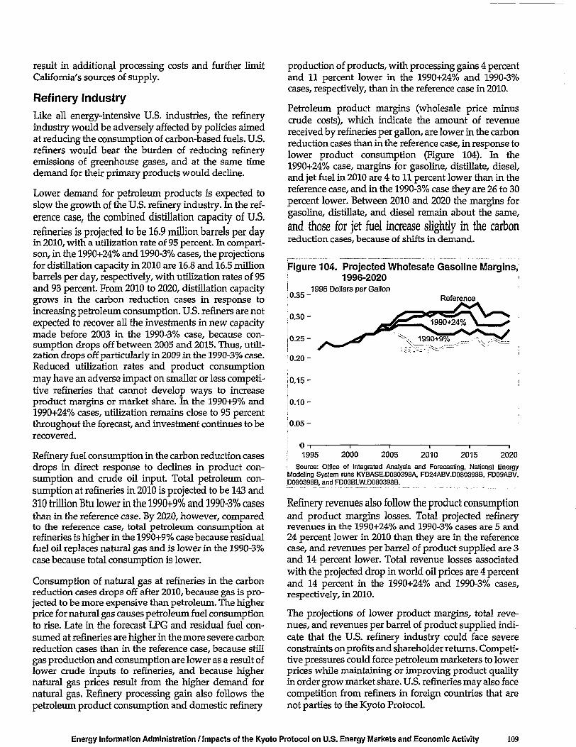
result in additional processing costs and further limitCalifornia's sources of supply.
Refinery IndustryLike all energy-intensive U.S. industries, the refineryindustry would be adversely affected by policies aimedat reducing the consumption of carbon-based fuels. U.S.refiners would bear the burden of reducing refineryemissions of greenhouse gases, and at the same timedemand for their primary products would decline.
Lower demand for petroleum products is expected toslow the growth of the U.S. refinery industry. In the ref-erence case, the combined distillation capacity of U.S.refineries is projected to be 16.9 million barrels per dayin 2010, with a utilization rate of 95 percent. In compari-son, in the 1990+24% and 1990-3% cases, the projectionsfor distillation capacity in 2010 are 16.8 and 16.5 millionbarrels per day, respectively, with utilization rates of 95and 93 percent. From 2010 to 2020, distillation capacitygrows in the carbon reduction cases in response toincreasing petroleum consumption. U.S. refiners are notexpected to recover all the investments in new capacitymade before 2003 in the 1990-3% case, because con-sumption drops off between 2005 and 2015. Thus, utili-zation drops off particularly in 2009 in the 1990-3% case.Reduced utilization rates and product consumptionmay have an adverse impact on smaller or less competi-tive refineries that cannot develop ways to increaseproduct margins or market share. In the 1990+9% and1990+24% cases, utilization remains close to 95 percentthroughout the forecast, and investment continues to berecovered.
Refinery fuel consumption in the carbon reduction casesdrops in direct response to declines in product con-sumption and crude oil input. Total petroleum con-sumption at refineries in 2010 is projected to be 143 and310 trillion Btu lower in the 1990+9% and 1990-3% casesthan in the reference case. By 2020, however, comparedto the reference case, total petroleum consumption atrefineries is higher in the 1990+9% case because residualfuel oil replaces natural gas and is lower in the 1990-3%case because total consumption is lower.
Consumption of natural gas at refineries in the carbonreduction cases drops off after 2010, because gas is pro-jected to be more expensive than petroleum. The higherprice for natural gas causes petroleum fuel consumptionto rise. Late in the forecast LPG and residual fuel con-sumed at refineries are higher in the more severe carbonreduction cases than in the reference case, because stillgas production and consumption are lower as a result oflower crude inputs to refineries, and because highernatural gas prices result from the higher demand fornatural gas. Refinery processing gain also follows thepetroleum product consumption and domestic refinery
production of products, with processing gains 4 percentand 11 percent lower in the 1990+24% and 1990-3%cases, respectively, than in the reference case in 2010.
Petroleum product margins (wholesale price minuscrude costs), which indicate the amount of revenuereceived by refineries per gallon, are lower in the carbonreduction cases than in the reference case, in response tolower product consumption (Figure 104). In the1990+24% case, margins for gasoline, distillate, diesel,and jet fuel in 2010 are 4 to 11 percent lower than in thereference case, and in the 1990-3% case they are 26 to 30percent lower. Between 2010 and 2020 the margins forgasoline, distillate, and diesel remain about the same,
and those for jet fuel increase slightly in the carbonreduction cases, because of shifts in demand.
Figure 104. Projected Wholesale Gasoline Margins,1996-2020
1996 Dollars per Gallonl 0 - 3 5 ~ Reference
0.30-
0.25-
0.20-
0.15-
0 .10-
0.05-
1995 2000 2005 2010 2015 2020
Source: Office of Integrated Analysis and Forecasting, National EnergyModeling System runs KYBASE.D080398A, FD24ABV.D080398B, FD09ABV.D080398B, and FD03BLW.D080398B.
Refinery revenues also follow the product consumptionand product margins losses. Total projected refineryrevenues in the 1990+24% and 1990-3% cases are 5 and24 percent lower in 2010 than they are in the referencecase, and revenues per barrel of product supplied are 3and 14 percent lower. Total revenue losses associatedwith the projected drop in world oil prices are 4 percentand 14 percent in the 1990+24% and 1990-3% cases,respectively, in 2010.
The projections of lower product margins, total reve-nues, and revenues per barrel of product supplied indi-cate that the U.S. refinery industry could face severeconstraints on profits and shareholder returns. Competi-tive pressures could force petroleum marketers to lowerprices while maintaining or improving product qualityin order grow market share. U.S. refineries may also facecompetition from refiners in foreign countries that arenot parties to the Kyoto Protocol.
Energy Information Administration / Impacts of the Kyoto Protocol on U.S. Energy Markets and Economic Activity 109
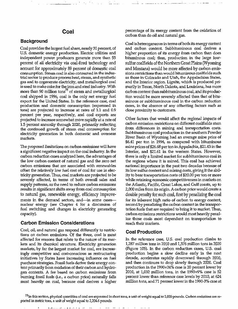
Coal
Background
Coal provides the largest fuel share, nearly 31 percent, ofU.S. domestic energy production. Electric utilities andindependent power producers generate more than 55percent of all electricity via coal-fired technology andaccount for approximately 89 percent of domestic coalconsumption. Steam coal is also consumed in the indus-trial sector to produce process heat, steam, and syntheticgas and to cogenerate electricity, and metallurgical coalis used to make coke for the iron and steel industry. Withmore than 90 million tons75 of steam and metallurgicalcoal shipped in 1996, coal is the only net energy fuelexport for the United States. In the reference case, coalproduction and domestic consumption (expressed intons) are projected to increase at rates of 1.1 and 0.9percent per year, respectively, and coal exports areprojected to increase somewhat more rapidly at a rate of1.5 percent annually through 2020, primarily reflectingthe continued growth of steam coal consumption forelectricity generation in both domestic and overseasmarkets.
The proposed limitations on carbon emissions will havea significant negative impact on the coal industry. In thecarbon reduction cases analyzed here, the advantages ofthe low carbon content of natural gas and the zero netcarbon emissions that are associated with renewablesoffset the relatively low fuel cost of coal for use in elec-tricity generation. Thus, coal markets are projected to beseverely affected, in terms of both overall sales andsupply patterns, as the need to reduce carbon emissionsresults in significant shifts away from coal consumptionto natural gas, renewable energy, efficiency improve-ments in the demand sectors, and—in some cases—nuclear energy (see Chapter 4 for a discussion offuel switching and changes in electricity generatingcapacity).
Carbon Emission Considerations
Coal, oil, and natural gas respond differently to restric-tions on carbon emissions. Of the three, coal is mostaffected for reasons that relate to the nature of its mar-kets and its chemical structure. Electricity generationmarkets, by far the largest market for coal, are increas-ingly competitive and cost-conscious as restructuringinitiatives by States have increasing influence on fuelpurchase strategies. Fossil fuels derive their energy con-tent primarily from oxidation of their carbon and hydro-gen contents. A fee based on carbon emissions fromburning fossil fuels (i.e., a carbon price) naturally fallsmost heavily on coal, because coal derives a higher
percentage of its energy content from the oxidation ofcarbon than do oil and natural gas.
Coal is heterogeneous in terms of both its energy contentand carbon content. Subbituminous coal derives ahigher proportion of its energy from carbon than doesbituminous coal; thus, production in the large low-sulfur coalfields of the Northern Great Plains (Wyomingand Montana) would be more affected by carbon emis-sions restrictions than would bituminous coalfields suchas those in Colorado and Utah, the Appalachian States,and the Interior region. Lignite, which is produced pri-marily in Texas, North Dakota, and Louisiana, has morecarbon content than subbituminous coal, and its produc-tion would be more severely affected than that of bitu-minous or subbituminous coal in the carbon reductioncases, in the absence of any offsetting factors such asclose proximity to customers.
Other factors that would affect the regional impacts ofcarbon emission restrictions on different coalfields stemfrom differences in mining and transportation costs.Subbituminous coal production in the southern PowderKiver Basin of Wyoming had an average mine price of$6.41 per ton in 1996, as compared with bituminousmine prices of $26.68 per ton in Appalachia, $21.43 in theInterior, and $21.61 in the western States. However,there is only a limited market for subbituminous coal inthe regions where it is mined. This coal has achievednational importance in the past two decades because ofits low sulfur content and mining costs, giving it the abil-ity to bear transportation costs of $20.00 per ton or morewhile retaining economic competitiveness in markets onthe Atlantic, Pacific, Great Lakes, and Gulf coasts, up to2,000 miles from its origin. A carbon price would create adouble penalty for such coal, first by penalizing the coalfor its inherent high ratio of carbon to energy content,second by penalizing the carbon content in the transpor-tation fuels that are required to bring it to market. Thus,carbon emissions restrictions would most heavily penal-ize those coals most dependent on transportation toreach their markets.
Coal Production
In the reference case, U.S. coal production climbs to1,287 million tons in 2010 and 1,376 million tons in 2020(Figure 105). In the carbon reduction cases, U.S. coalproduction begins a slow decline early in the nextdecade, accelerates rapidly downward through 2010,and then continues to drop slowly through 2020. Coalproduction in the 1990+24% case is 20 percent lower by2010, at 1,032 million tons, in the 1990+9% case is 52percent lower than reference case levels by 2010, at 624million tons, and 71 percent lower in the 1990-3% case at
75In this section, physical quantities of coal are expressed in short tons, a unit of weight equal to 2,000 pounds. Carbon emissions are re-ported in metric tons, a unit of weight equal to 2,204.6 pounds.
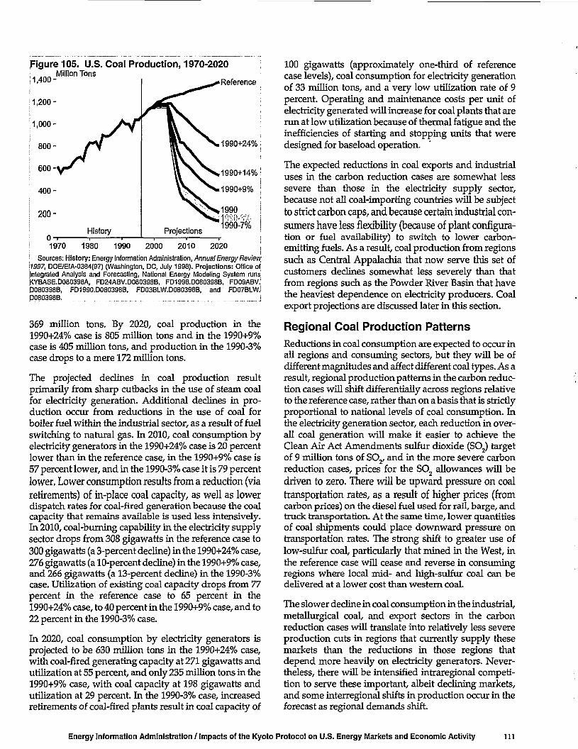
JFigure 105. U.S. Coal Production, 1970-2020Million Tons
• Reference
1990+24%
1990+14%
1990+9%
1990
1990-7%
1970 1980 1990 2000 2010 2020Sources: History: Energy Information Administration, Annual Energy Review
\1997, DOE/EIA-0384(97) (Washington, DC, July 1998). Projections: Office ofIntegrated Analysis and Forecasting, National Energy Modeling System runs)<YBASE.D080398A, FD24ABV.D080398B, FD1998.D080398B, FD09ABV.'D080398B, FD1990.D080398B, FD03BLW.D080398B, and FD07BLW.PP80398B.
369 million tons. By 2020, coal production in the1990+24% case is 805 million tons and in the 1990+9%case is 405 million tons, and production in the 1990-3%case drops to a mere 172 million tons.
The projected declines in coal production resultprimarily from sharp cutbacks in the use of steam coalfor electricity generation. Additional declines in pro-duction occur from reductions in the use of coal forboiler fuel within the industrial sector, as a result of fuelswitching to natural gas. In 2010, coal consumption byelectricity generators in the 1990+24% case is 20 percentlower than in the reference case, in the 1990+9% case is57 percent lower, and in the 1990-3% case it is 79 percentlower. Lower consumption results from a reduction (viaretirements) of in-place coal capacity, as well as lowerdispatch rates for coal-fired generation because the coalcapacity that remains available is used less intensively.In 2010, coal-burning capability in the electricity supplysector drops from 308 gigawatts in the reference case to300 gigawatts (a 3-percent decline) in the 1990+24% case,276 gigawatts (a 10-percent decline) in the 1990+9% case,and 266 gigawatts (a 13-percent decline) in the 1990-3%case. Utilization of existing coal capacity drops from 77percent in the reference case to 65 percent in the1990+24% case, to 40 percent in the 1990+9% case, and to22 percent in the 1990-3% case.
In 2020, coal consumption by electricity generators isprojected to be 630 million tons in the 1990+24% case,with coal-fired generating capacity at 271 gigawatts andutilization at 55 percent, and only 235 million tons in the1990+9% case, with coal capacity at 198 gigawatts andutilization at 29 percent. In the 1990-3% case, increasedretirements of coal-fired plants result in coal capacity of
100 gigawatts (approximately one-third of referencecase levels), coal consumption for electricity generationof 33 million tons, and a very low utilization rate of 9percent. Operating and maintenance costs per unit ofelectricity generated will increase for coal plants that arerun at low utilization because of thermal fatigue and theinefficiencies of starting and stopping units that weredesigned for baseload operation.
The expected reductions in coal exports and industrialuses in the carbon reduction cases are somewhat lesssevere than those in the electricity supply sector,because not all coal-importing countries will be subjectto strict carbon caps, and because certain industrial con-sumers have less flexibility (because of plant configura-tion or fuel availability) to switch to lower carbon-emitting fuels. As a result, coal production from regionssuch as Central Appalachia that now serve this set ofcustomers declines somewhat less severely than thatfrom regions such as the Powder River Basin that havethe heaviest dependence on electricity producers. Coalexport projections are discussed later in this section.
Regional Coal Production PatternsReductions in coal consumption are expected to occur inall regions and consuming sectors, but they will be ofdifferent magnitudes and affect different coal types. As aresult, regional production patterns in the carbon reduc-tion cases will shift differentially across regions relativeto the reference case, rather than on a basis that is strictlyproportional to national levels of coal consumption. Inthe electricity generation sector, each reduction in over-all coal generation will make it easier to achieve theClean Air Act Amendments sulfur dioxide (SO2) targetof 9 million tons of SO2, and in the more severe carbonreduction cases, prices for the SO2 allowances will bedriven to zero. There will be upward pressure on coaltransportation rates, as a result of higher prices (fromcarbon prices) on the diesel fuel used for rail, barge, andtruck transportation. At the same time, lower quantitiesof coal shipments could place downward pressure ontransportation rates. The strong shift to greater use oflow-sulfur coal, particularly that mined in the West, inthe reference case will cease and reverse in consumingregions where local mid- and high-sulfur coal can bedelivered at a lower cost than western coal.
The slower decline in coal consumption in the industrial,metallurgical coal, and export sectors in the carbonreduction cases will translate into relatively less severeproduction cuts in regions that currently supply thesemarkets than the reductions in those regions thatdepend more heavily on electricity generators. Never-theless, there will be intensified intraregional competi-tion to serve these important, albeit declining markets,and some interregional shifts in production occur in theforecast as regional demands shift.
Energy Information Administration / Impacts of the Kyoto Protocol on U.S. Energy Markets and Economic Activity 111

In the reference case, the western share of total U.S. coalproduction increases from 47 percent in 1996 to 57percent in 2010, as a result of its lower cost and thegrowing requirements for low-sulfur coal under theClean Air Act Amendments (Figure 106). In contrast, thewestern share in the carbon reduction cases decreases to54 percent in the 1990+24% case, to 39 percent in the1990+9% case, and to 28 percent in the 1990-3% case in2010. Approximately 75 percent of the 179 million tonreduction in western coal production in the 1990+24%case, 486 million ton reduction in the 1990+9% case, andthe 628 million ton reduction in the 1990-3% case isborne by subbituminous surface mines in the PowderRiver Basin. The low-sulfur coal from these surfacemines is used almost exclusively for electricitygeneration and must be transported over relatively longdistances to reach many of the markets that are projectedto expand in the reference case.
As overall demand falls, eastern minemouth prices arereduced, and there is less economic incentive totransport western coal. Western coal becomes lesscompetitive in electricity generation markets as trans-portation fuel costs increase, and its potential to expandinto most industrial and export applications is limitedby its lower heat content and other physical characteris-tics, such as moisture content and handling problems.
By 2020, western coal production has dropped by anadditional 189 million tons from 2010 levels in the1990+24% case, 115 million tons in the 1990+9% case,and by 71 million tons in the 1990-3% case, with westernproduction shares reaching 45, 32, and 19 percent,respectively. In these cases, the limited coal that isproduced in the West is generally sold in markets closeto the point of production.
Figure 106. Western Share of U.S. CoalProduction, 1990-2020
Percent Share
•Reference •1990+24%7 0 -
6 0 -1990+9% • 1990-3%
1990 1996 2000 2005 2010 2015 2020Sources: History: Energy Information Administration, Annual Energy fiev/ewf
'{1997, DOE/EIA-0384(97) (Washington, DC, July 1998). Projections: Office ofIntegrated Analysis and Forecasting, National Energy Modeling System runsKYBASE.D080398A, FD24ABV.D080398B, FD09ABV.D080398B, andFD03BLW.D080398B.
Coal PricesBecause coal is heterogeneous in terms of heat content,sulfur level, and other physical properties, trends innational average prices are affected substantially by therelative shares of the various coal types produced andsold and by the units in which prices are reported. Forexample, coal from the Powder River Basin is generallythe lowest-priced coal per ton on a minemouth basis;however, because Powder River Basin coal has roughlytwo-thirds the heat content of bituminous coal, its costadvantage is somewhat less on a Btu basis and may benonexistent when delivered to more distant markets.
In general, to the extent that market share shifts awayfrom Powder River Basin coal, which has a low mine-mouth price, to higher-priced bituminous coal, thenational average minemouth price will increase. Simi-larly, the greater the share represented by metallurgicalcoal and by premium grades of coal for export use, thehigher will be the share-weighted average price. Thiscompositional effect offsets the reduction in minemouthprices at the regional level that is likely to occur becauseof intraregional competition and the lower productionquantities that occur when carbon restrictions takeeffect. The regional productivity improvements pro-jected in the reference case are assumed to occur at thesame rates in all the carbon reduction cases given thesame rate of technological progress. However, if thelevel of investment in new capital equipment is severelyconstrained, there could be adverse impacts on produc-tivity.
In 2010, real minemouth prices are projected to decreaseto $14.29 per ton in the reference case but increase to$14.72 in the 1990+24% case, to $16.42 in the 1990+9%case, and to $17.90 in the 1990-3% case (Figure 107).Minemouth prices in individual regions generallydecline in all cases, but the national average minemouthprice increases in the carbon reduction cases because ofthe shift in quantity shares to higher grade and higherpriced coal and away from coal with a lower minemouthprice, such as that from the Powder River Basin. In someinstances, however, even the regional weighted averageprice for a given coal rank will increase relative to thereference case, if a greater share of coal is being shippedto export or metallurgical markets that demandpremium-grade (and therefore higher priced) coals. Thepattern of higher national average prices in the carbonreduction cases is accentuated by the projections for2020, when prices increase from the reference case valueof $12.53 to $14.29 in the 1990+24% case, to $16.24 in the1990+9% case, and to $19.63 in the 1990-3% case.
Delivered prices for coal, as projected in this report,reflect the sum of the minemouth price, transportationcost (in dollars per ton), and the carbon price associatedwith meeting a carbon reduction target. The carbonprice dominates the effects on delivered prices in the
112 Ener Information A<
Figure 107. Average U.S. Minemouth Coal Prices,1970-2020
50
40
30
20
10
n
1996 Dollars per Ton
\
) V-
History
—Reference
— 1990+24%
— 1990+14%
—1990+9%
— 1990
I'lMIt 1 %
-1990-7%
-C-^=— .
Projections
1970 1980 1990 2000 2010 2020
\ Note: Carbon prices are added to the delivered price of coal, not tofhe minemouth price. [
Sources: History: Energy Information Administration, Annual Energy Review[1997, DOE/EIA-0384(97) (Washington, DC, July 1998). Projections: Office ofIntegrated Analysis and Forecasting, National Energy Modeling System runs|<YBASE.D080398A, FD24ABV.D080398B, FD1998.D080398B, FD09ABVJP080398B, FD1990.D080398B, FD03BLW.D080398B, and FD07BLW.'D080398B. _ __!
carbon reduction cases. In 2010, the carbon fee adds$1.73 per million Btu to the delivered price of coal toelectricity generators in the 1990+24% case, $4.18 permillion Btu in the 1990+9% case, and $7.51 per millionBtu in the 1990-3% case. In 2020, the carbon price compo-nent drops to $2.55, $3.62, and $6.14 per million Btu,respectively because the carbon price for all fuels islower in 2020.
In 2010, the national average delivered price of coal toelectricity generators increases from $22.20 per ton in thereference case to $57.03 in the 1990+24% case, $109.56 inthe 1990+9% case, and $185.47 in the 1990-3% case (Fig-ure 108). In 2020, the delivered price to electricity gen-erators rises from $19.56 in the reference case, to $71.95in the 1990+24% case, to $95.33 in the 1990+9% case, andto $156.60 in the 1990-3% case.
Coal Industry Employment andProductivity
Between 1978 and 1996, the number of miners employedin the U.S. coal industry fell by 5.8 percent a year, declin-ing from 246,000 to 83,000. The decrease primarilyreflected strong growth in labor productivity, whichincreased at an annual rate of 6.7 percent over the sameperiod. An additional factor was increased output fromlarge surface mines in the Powder River Basin, whichrequire much less labor per ton of output than mineslocated in the Interior and Appalachian regions. ThePowder River Basin share of total U.S. coal productionincreased from 13 percent in 1978 to 30 percent in 1996.
1996 Dollars per Ton250-
History
200-
150-
100-
50- / ^ - * S s ^
0-i • 1
Projections
A
Figure 108. Coal Prices to Electricity Generators,1970-2020
1990-7%
1990
1990+9%
1990+14%
1990+24%
Reference
1970 1980 1990 2000 2010 2020
Sources: History: Energy Information Administration, Annual Energy Review1997, DOE/EIA-0384(97) (Washington, DC, July 1998). Projections: Office of.integrated Analysis and Forecasting, National Energy Modeling System runsKYBASE.D080398A, FD24ABV.D080398B, FD1998.D080398B, FD09ABV.JD080398B, FD199D.D080398B, FD03BLW.D080398B, and FD07BLWJb080398B. ]
In the reference case, productivity improvements areassumed to continue but to decline in magnitude overthe forecast period. On a national basis, labor productiv-ity increases at an average rate of 2.3 percent a year overthe whole forecast. The annual rate of increase slows,however, from 5.8 percent in 1996 to approximately 1.6percent per year from 2010 to 2020. With improvementscontinuing over the forecast period, further declines inemployment of 1.3 and 1.1 percent per year are projectedfrom 1996 through 2010 and from 2010 through 2020,respectively. In absolute terms, coal mine employmentdeclines from 83,000 in 1996 to 69,000 in 2010 and to62,000 in 2020.
Regionally, labor productivity in the carbon reductioncases is assumed to improve at the same rates as in thereference case. As a result, lower levels of productionin the carbon reduction cases in all supply regions, rela-tive to the reference case, result in lower employmentlevels in all regions. Table 23 shows projections of coalmining jobs in 2010 by region for the reference case andthe carbon reduction cases. In the 1990+24% case, coalmine employment declines at a rate of 2.5 percent a yearbetween 1996 and 2010, falling from 83,000 in 1996 to58,000 in 2010 (Figure 109). In the 1990+9% case, employ-ment declines at a more rapid rate of 4.6 percent a year to2010, resulting in employment of only 43,000 miners in2010. In the 1990-3% case, coal mine employmentdeclines at a rate of 7.2 percent a year between 1996 and2010, reaching 29,000 in 2010.
Production and employment are positively correlated.In 2010, the projected levels of coal production in the
^Higher or lower rates of productivity growth could occur in the carbon reduction cases depending on the skill level and motivation ofthe labor force in a rapidly contracting job market and the rate at which new capital equipment and technology are adopted.
Energy Information Administration / Impacts of the Kyoto Protocol on U.S. Energy Markets and Economic Activity 113

[Table 23. Projected Number of Coal Mining Jobs by Region, 2010Region 1996 I Reference [ 1990+24% [ 1990+14% | 1990+9% I 1990 | 19903% | 1990-7%
S Appalachia
i Interior1'Powder River Basin0
Other Westd
U.S. Total
60,00113,4774,1595,825
83,462
49,477
8,043
5,013
5,693
68,519
41,617
7,801
3,827
4,785
58,223
37,340
7,617
2,490
2,859
50,224
32,3866,2571,8292,254
42,531
26,0344,3151,0151,034
32,053
24,3073,484844941
29,187
21,6542,663673895
25,486
*PA, OH, MD, WV, VA, and KY (east).bIL, IN, KY (west), IA, MO, KS, AR, OK, TX, and LA.CWY, MT, and ND.dCO, UT, NM, AZ, AK, and WA. jSource: History: Energy Information Administration, Coal Industry Annual 1996, DOE/EIA-584(96) (Washington, DC, November 1997). Projections: Office of Intej
grated Analysis and Forecasting, National Energy Modeling System runs KYBASE.D080398A, FD24ABV.D080398B, FD1998.D080398B, FD09ABV.D080398BFD1990.D080398B, FD03BLW.D080398B, FD07BLW.D080398B. i
Figure 109. Coal Mine Employment, 1970-2020Number of Mining Jobs
250.000- *
200,000 / 1
/ * \
150,000 -«/"* \
\
100,000 - ^ ^
50,000 -
n —. , ,
Projections
••Reference
— 1990+24%
—1990+14%
—1990+9%
— 1990
t=> 1990-3%
=1990-7%
1970 1980 1990 2000 2010 2020Sources: History: Energy Information Administration (EIA), The U.S. Coal
Industry, 1970-1990: Two Decades of Change, DOE/EIA-0559, (Washington,'DC, November 1992) and EIA, Coal Industry Annual 1996, DOE/ElA-0584(96)'(Washington, DC, November 1997). Projections: Office of Integrated Analysisand Forecasting, National Energy Modeling System runs KYBASE.D080398AJFD24ABV.D080398B, FD1998.D080398B, FD09ABV.D080398B, FD1990.'D080398B, FD03BLW.D080398B, and FD07BLW.D080398B. j
1990+24% and 1990-3% cases are 20 percent and 75percent lower, respectively, than in the reference case. Incomparison, employment in the 1990+24% case is only15 percent lower in 2010 than in the reference case andemployment in the 1990-3% case in 2010 is only 57percent below the reference case. The projected declinesin employment are smaller than the declines inproduction because of the relatively greater losses inoutput projected from mines in the Northern GreatPlains, which require less labor per unit of output thanmines in other coal-producing regions.
Table 24 provides an indication of the importance of coalindustry jobs in the top coal-producing States. The tableshows that the wages associated with coal miningexceeded 2 percent of all wages paid in 1996 in WestVirginia, Kentucky, and Wyoming. In West Virginia andWyoming, they accounted for more than 5 percent of allwages paid. The fact that coal mining wages are higherthan average wages in these States is shown by the factthat coal industry jobs account for a greater share of total
wages than their share of total employment. In WestVirginia, the coal industry employs 3.2 percent of allworkers in the State but accounts for 6.5 percent of allwages paid. In Wyoming, coal industry workers accountfor only 2.2 percent of all jobs but earn 5.3 percent of allwages. Similarly, in Kentucky, the coal industryprovides 1.2 percent of all jobs but 2.1 percent of allwages. Table 24 also shows that while the potential fordirect losses of coal-related wages and employment isconcentrated in the 10 States listed, it is much morestrongly concentrated in West Virginia, Kentucky,Wyoming, and perhaps Pennsylvania (depending onwhether the absolute amount of wages and employmentat stake is counted, or the relative proportion of theState's total wages and employment).
In addition to the substantial contraction of the U.S. coalindustry projected in the carbon reduction cases, theU.S. rail industry, which derives considerable revenuesfrom coal shipments, also stands to be greatly affected(see box).
U.S. Coal ExportsU.S. coal producers exported 90 million tons of coal in1996. Of that amount, 59 percent represented shipmentsof coking coal for use at integrated steel plants world-wide, and 41 percent was steam coal, used primarily forelectricity generation and for the production of processsteam and direct heat for industrial applications. In 1997,U.S. coal exports fell by 7 million tons, reversing theupward trend of the previous 2 years. The decline wasmostly in steam coal exports, as a result of weak interna-tional coal prices and strong competition from othercoal-exporting countries.
In the reference case, U.S. coal exports are projectedto increase from 90 million tons in 1996 to 113 milliontons in 2010. All the increase reflects expected growthin steam coal exports, with exports of metallurgical coalprojected to decline slightly. In the reference case, worldmetallurgical coal trade remains relatively constant,although regionally there is a slight shift awayfrom markets in Europe and Japan to Brazil and the

[Table 24. Coal Industry Wages and Employment, 1996
State
Wages
Million 1996 Dollars Percent of State Total
Employment
Number of Jobs | Percent of State Total
i West Virginia .
I Kentucky
| Wyoming
I Pennsylvania .
! Illinois
[ Virginia
Alabama
Ohio
Texas
Montana
Subtotal
United States.
1,041
815
258
512
347
290
332
172
149
49
3,965
4,691
6.53
2.06
5.29
0.34
0.20
0.03
0.74
0.12
0.65
0.66
0.42
0.17
21,033
19,372
4,706
11,214
6,136
7,039
6,552
3,889
2,861
933
83,375
97,649
3.17
1.20
2.20
0.22
0.11
0.02
0.04
0.01
<0.01
0.03
0.03
0.08
I aRelative to Form EIA-7A, "Coal Production Report," which focuses on workers directly involved in the production and preparation of coal, the datapresented in this table include coverage of corporate officials, executives, clerical workers, and other office workers. Data from Form EIA-7A indicate;that 83,462 miners were employed in the U.S. coal industry in 1996.
Source: U.S. Department of Labor, Bureau of Labor Statistics, ES-202 Program, "Covered Employment and Wages."
developing countries in Asia. World steam coal trade isprojected to increase by 45 percent between 1996 and2010, rising from 305 million tons to 441 million tons.The U.S. share of total world coal trade is projected toremain constant at about 18 percent.
In the reference case, Japan's remaining two coal minesare assumed to be closed shortly after 2000. Currentlythese mines have a combined annual production capac-ity of about 3.5 million tons, representing less than 3 per-cent of Japan's total coal consumption. In 1996, coalconsumption in Japan amounted to 144 million tons—82million tons of steam coal (including 9.5 million tons ofcoal for pulverized coal injection at blast furnaces) and62 million tons of coking coal.
In the carbon reduction cases, two alternative coal tradescenarios were developed. In a severe carbon reductioncase (1990-3%), carbon emissions in Western Europewere assumed to be 8 percent below their 1990 level by2010 consistent with the limits for the European Unionthat were specified in the Kyoto Protocol. Similarly, car-bon emissions in Japan were assumed to be 6 percentbelow their 1990 level by 2010. Coal was assumed to playa proportionately greater role than oil or natural gas inmeeting these emission reductions, because it has ahigher carbon content (on a Btu basis) and the opportu-nities to substitute for petroleum products in the trans-portation sector are limited. In Western Europe, bothdomestic coal production and imports were assumed todecline by approximately 50 percent, but in Japan coalimports had to account for the total reduction in coalconsumption.
In Europe, steam coal imports from all sources arereduced from 156 million tons in the reference case in2010 to 47 million tons in the 1990-3% case. Only steamcoal imports to the industrialized Annex I countries inEurope are reduced. Steam coal imports to Japan, theonly Annex I country in Asia, are reduced from 99 mil-lion tons in the reference case in 2010 to 56 million tons inthe 1990-3% case. Because other fuels are not easily sub-stituted for coal coke at steel plants, coking coal importsare not adjusted downward.
Steam coal imports to Japan are reduced by a relativelysmaller amount than are imports to Europe, primarilybecause Japan has limited access to alternative sourcesof energy such as natural gas and renewable fuels. Inaddition to reduced use of coal, other strategies thatJapan may pursue to meet its carbon reduction targetsinclude purchasing surplus emission allowances fromother signatory countries and pursuing an acceleratednuclear program.77
U.S. coal exports to Europe and Asia in 2010 are pro-jected to be lower by 27 and 7 million tons, respectively,in the 1990-3% case (and all other carbon reduction caseswhere U.S. carbon emissions are held at or below the1990 level in 2010) than in the reference case. In thesecases, U.S. coal exports are projected to decline to 76 mil-lion tons in 2010.
In the moderate cases, 1990+24% and 1990+9%, devel-oped to evaluate the potential impacts of less severereductions in carbon emissions, Western European coalconsumption and imports were assumed to decline by asmaller amount than in the severe case discussed above,
^ I n June 1998, a panel headed by then Prime Minister Ryutaro Hashimoto urged the government to construct an additional 20 new nu-clear plants over the next 12 years, with the goal of increasing Japan's nuclear generation by more than 50 percent between 1997 and 2010.EIA's International Energy Outlook (IEO98) high nuclear case projects an increase of 12.4 gigawatts (29 percent) in Japan's nuclear generatingcapacity over the same period. The IEO98 reference case projects an increase of only 5.2 gigawatts (12 percent) between 1996 and 2010.
Energy Information Administration / Impacts of the Kyoto Protocol on U.S. Energy Markets and Economic Activity 115
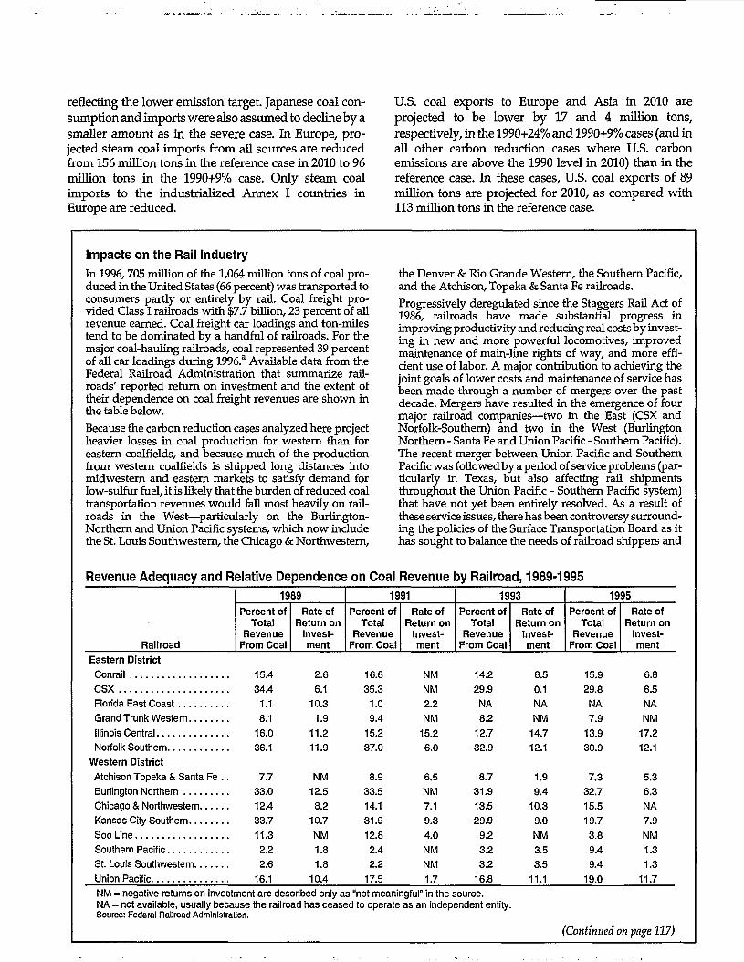
reflecting the lower emission target. Japanese coal con-sumption and imports were also assumed to decline by asmaller amount as in the severe case. In Europe, pro-jected steam coal imports from all sources are reducedfrom 156 million tons in the reference case in 2010 to 96million tons in the 1990+9% case. Only steam coalimports to the industrialized Annex I countries inEurope are reduced.
U.S. coal exports to Europe and Asia in 2010 areprojected to be lower by 17 and 4 million tons,respectively, in the 1990+24% and 1990+9% cases (and inall other carbon reduction cases where U.S. carbonemissions are above the 1990 level in 2010) than in thereference case. In these cases, U.S. coal exports of 89million tons are projected for 2010, as compared with113 million tons in the reference case.
Impacts on the Rail Industry
In 1996,705 million of the 1,064 million tons of coal pro-duced in the United States (66 percent) was transported toconsumers partly or entirely by rail. Coal freight pro-vided Class I railroads with $7.7 billion, 23 percent of allrevenue earned. Coal freight car loadings and ton-milestend to be dominated by a handful of railroads. For themajor coal-hauling railroads, coal represented 39 percentof all car loadings during 1996.a Available data from theFederal Railroad Administration that summarize rail-roads' reported return on investment and the extent oftheir dependence on coal freight revenues are shown inthe table below.
Because the carbon reduction cases analyzed here projectheavier losses in coal production for western than foreastern coalfields, and because much of the productionfrom western coalfields is shipped long distances intomidwestern and eastern markets to satisfy demand forlow-sulfur fuel, it is likely that the burden of reduced coaltransportation revenues would fall most heavily on rail-roads in the West—particularly on the Burlington-Northern and Union Pacific systems, which now includethe St. Louis Southwestern, the Chicago & Northwestern,
the Denver & Rio Grande Western, the Southern Pacific,and the Atchison, Topeka & Santa Fe railroads.
Progressively deregulated since the Staggers Rail Act of1986, railroads have made substantial progress inimproving productivity and reducing real costs by invest-ing in new and more powerful locomotives, improvedmaintenance of main-line rights of way, and more effi-cient use of labor. A major contribution to achieving thejoint goals of lower costs and maintenance of service hasbeen made through a number of mergers over the pastdecade. Mergers have resulted in the emergence of fourmajor railroad companies—two in the East (CSX andNorfolk-Southern) and two in the West (BurlingtonNorthern - Santa Fe and Union Pacific - Southern Pacific).The recent merger between Union Pacific and SouthernPacific was followed by a period of service problems (par-ticularly in Texas, but also affecting rail shipmentsthroughout the Union Pacific - Southern Pacific system)that have not yet been entirely resolved. As a result ofthese service issues, there has been controversy surround-ing the policies of the Surface Transportation Board as ithas sought to balance the needs of railroad shippers and
Revenue Adequacy and Relative Dependence on Coal Revenue by Railroad, 1989-1995
Railroad
1989
Percent ofTotal
RevenueFrom Coal
Rate ofReturn on
Invest-ment
1991
Percent ofTotal
RevenueFrom Coal
Rate ofReturn on
Invest-ment
1993
Percent ofTotal
RevenueFrom Coal
Rate ofReturn on
Invest-ment
1995
Percent ofTotal
RevenueFrom Coal
Rate ofReturn on
Invest-ment
Eastern District
Conrail 15.4 2.6 16.8 NM 14.2 6.5 15.9 6.8
CSX 34.4 6.1 35.3 NM 29.9 0.1 29.8 6.5
Florida East Coast 1.1 10.3 1.0 2.2 NA NA NA NA
Grand Trunk Western 8.1 1.9 9.4 NM 8.2 NM 7.9 NM
Illinois Central 16.0 11.2 15.2 15.2 12.7 14.7 13.9 17.2
Norfolk Southern 36.1 11.9 37.0 6.0 32.9 12.1 30.9 12.1
Western District
Atchison Topeka & Santa F e . . 7.7 NM 8.9 6.5 8.7 1.9 7.3 5.3
Burlington Northern 33.0 12.5 33.5 NM 31.9 9.4 32.7 6.3
Chicago & Northwestern 12.4 8.2 14.1 7.1 13.5 10.3 15.5 NA
Kansas City Southern 33.7 10.7 31.9 9.3 29.9 9.0 19.7 7.9
SooLine 11.3 NM 12.8 4.0 9.2 NM 3.8 NM
Southern Pacific 2.2 1.8 2.4 NM 3.2 3.5 9.4 1.3
St. Louis Southwestern 2.6 1.8 2.2 NM 3.2 3.5 9.4 1.3
Union Pacific 16.1 1O4 VT£ 1 J 1&8 11J 1^0 11.7
NM = negative returns on investment are described only as "not meaningful" in the source.NA = not available, usually because the railroad has ceased to operate as an independent entity.Source: Federal Railroad Administration.
(Continued on page 117)

Impacts on the Rail Industry (Continued)the continued profitability of the Union Pacific, and of theNation's major railroads in general. Even if these issuesare successfully resolved over the next few years, theadoption of carbon emissions restrictions would inevita-bly result in a reduction in domestic coal traffic handledby the railroads.As suggested by the results of the carbon reduction cases,the reductions in coal traffic range from moderate tosevere, depending on the case. In all cases, western coal,particularly subbituminous coal from the Powder RiverBasin, would be most severely restricted, because of itsdependence on long-distance rail transportation to reachits markets in locations up to 2,000 miles away and itshigh ratio of carbon to energy content. As shown in thetable, the Burlington Northern and Union Pacific systemshave a fairly high dependence on coal freight revenue;therefore, the loss of revenue associated with carbon
reduction measures could create significant financialproblems for those firms. Lignite production in Texas,Louisiana, and North Dakota would also be severelyreduced by carbon emissions restrictions, but the effect onrail revenues would be minor. Because of its inherentlylow heat content, lignite is predominantly consumed at orclose to the place of mining.Although the projected losses of coal production in theindividual carbon reduction cases are proportionatelyand absolutely less for Appalachian coalfields thanfor thePowder River Basin, the two eastern rail systems (CSXand Norfolk Southern) are also highly dependent on coalrevenue. In the more severe carbon reduction cases,Appalachian coal production could be reduced by one-third to one-half, with potentially serious financial conse-quences for these carriers.
aAssociation of American Railroads, Freight Commodity Statistics.
Energy Information Administration / Impacts of the Kyoto Protocol on U.S. Energy Markets and Economic Activity 117

This page is intentionally left blank.

6. Assessment of Economic Impacts
Objectives of theMacroeconomic Analysis
Because energy resources are used to produce mostgoods and services, higher energy prices can affect theeconomy's production potential. Since the energy crisisof the 1970s, economic research has led to a better under-standing of the potential adverse economic conse-quences of rising real energy costs, in terms of both long-run equilibrium costs and short-run adjustment costs.Long-run equilibrium costs are associated with reduc-ing reliance on energy in favor of other factors of pro-duction—including labor and capital, which becomerelatively cheaper as energy costs rise. Short-run adjust-ment costs, or business cycle costs, can arise when priceincreases disrupt capital or employment markets. Long-run costs are considered unavoidable. Short-run costsmight be avoidable if price changes can be accuratelyanticipated or if appropriate compensatory monetaryand fiscal policies can be implemented.
This chapter assesses possible impacts on the economyassociated with attaining the alternative carbon mitiga-tion targets presented earlier in this report, focusing onthree target cases—the 3-percent-below-1990 (1990-3%),the 9-percent-above-1990 (1990+9%), and the 24-percent-above-1990 (1990+24%) cases—and comparingthem with a reference case that does not include theKyoto Protocol. In evaluating these alternative targets,three key questions are posed:
• What would be the unavoidable minimum impacton the economy?
• With rising energy prices and inflation, what cyclicalreactions could the economy face, and how wouldthe Federal Reserve Board implement accommodat-ing monetary policy?
• What would be the impact of fiscal policy on eco-nomic output and inflation?
EIA used the Data Resources, Inc. (DRI) model of theU.S. economy to assess these issues. 8 The DRI model isa representation of the U.S. economy with detailedoutput, price, and financial sectors incorporating bothlong-term and short-term properties. In the DRI model,the concept of potential GDP reflects the trajectory of thelong-term growth potential of the economy at fullemployment, while actual GDP is a measure of the tran-sition effects as the economy adjusts to its long-run path.Energy end-use demands and prices for fuels are the keyenergy inputs to the DRI model. In addition, for thisanalysis, assumptions were made about the domesticflow of funds that would result from a U.S. system ofcarbon permits sold by the Federal Government, andabout the international flow of funds that would resultfrom international trading of permits. These assump-tions were based on the results of the energy marketanalyses described in the preceding chapters of thisreport.
This chapter first presents a discussion of the U.S. permitsystem and the potential role of international trading ofpermits. A summary of the macroeconomic effects ispresented next, focusing on the definition and measure-ment of -potential GDP, actual GDP, and the value of thepurchased international permits as key elements. The chap-ter then discusses in detail two topics. The firstaddresses the unavoidable loss to the economy thatwould result from a reduction in available energyresources. The unavoidable loss has two components:the loss in potential GDP and the value of the purchasedinternational permits. The chapter concludes with a dis-cussion of the possible transitional impacts on the aggre-gate economy that might occur as energy prices increasein response to carbon emission constraints. The criticalroles of monetary and fiscal policy are highlighted. Twofiscal policies are considered as alternative methods ofreturning carbon permit revenues to the economy:through a lump sum personal income tax rebate andthrough a social security tax rebate that would passfunds back to both employers and employees.
78The version of the model used is US97A95.^This macroeconomic analysis of the costs of implementing the Kyoto Protocol is limited to the consideration of investment costs that
are comparable in magnitude to those in the reference case, as well as direct fuel costs. No consideration is given to the potential incrementalcosts of investment in technology and infrastructure that would be necessaiy in each of the specific cases analyzed. Business investmentsabove reference case levels may be required to reduce energy costs in response to increasing energy prices.
Energy Information Administration / Impacts of the Kyoto Protocol on U.S. Energy Markets and Economic Activity 119
The U.S. Permit System andInternational Trading of Permits
Two key features shape the discussion in this chapter—first, the characterization of the carbon permit tradingsystem as an auction run by the Federal Government;and second, the international trading of carbon permits.Both of these issues have important implications for theassessment of the potential macroeconomic impacts ofcarbon mitigation policies.
The U.S. Permit System
When a system is developed for the trading of carbonpermits within the United States, a number of initialdecisions must be made: How many permits will beavailable? Will they be freely allocated or sold by com-petitive auction? If they are allocated, how will the initialallocations be made? If they are sold, what will be donewith the revenues? How many permits will be bought ininternational markets? If the permits are traded in a freemarket, holders of permits who can reduce carbon emis-sions at a cost below the permit price will sell their per-mits, and those with higher costs of reduction will buypermits, resulting in a transfer of funds between privateparries. If the permits are sold by competitive auction,there will be a transfer of funds from emitters of carbonto the Federal treasury.
This analysis makes the explicit assumption that carbonpermits will be sold in a competitive auction run by theFederal Government.80 To illustrate the importance ofrecycling the funds back to the economy, two fiscal pol-icy approaches are considered: first, returning collectedrevenues to consumer through personal income taxrebates and, second, lowering the social security tax rateas it applies to both employers and employees. The twopolicies are meant only to be representative of a set ofpossible fiscal policies that might accompany an initialcarbon mitigation policy.
International Trading of PermitsIn the energy market assessments described earlier inthis report, the projected carbon prices reflect the pricethe United States would be willing to pay to achieve agiven emissions reduction target. The more stringent thecarbon target, the higher the carbon price. The energymarket analysis in this report does not address the inter-national implications of achieving a particular target atthe projected carbon price. In the absence of modeling
international trade of emissions permits, the energymarket assessment makes no link between the U.S. car-bon price and the international market-clearing price ofpermits, or the price at which other countries would bewilling to offer permits for sale in the United States.
The macroeconomic analysis in this chapter departsfrom the above interpretation in order to facilitate anevaluation of the role of the purchase of permits in aninternational market. The analysis first assumes that theU.S. State Department's assessment of the accounting ofcarbon-absorbing sinks and offsets from reductions inother greenhouse gases will reduce the binding U.S.emissions target to 3 percent below the 1990 level ofemissions. Then, if the United States is to meet a targetthat is less stringent, the difference in emissions isassumed to be made up through the purchase of permitson the international market. Moreover, the United Statesis assumed to purchase international permits at the mar-ginal abatement cost in the United States. Thus, the domes-tic carbon price would be the same as the internationalpermit price under the alternative targets considered. Ifunrestricted international trading among Annex I coun-tries is allowed, the international carbon price could fallbelow the levels projected here for domestic permits. Ifthis were to occur, to achieve equilibrium in an uncon-strained market for carbon permits, the domestic carbonprice would fall to the international carbon price.
The above assumptions imply that different inter-national supplies of permits would be available in thealternative cases considered. This is an importantsimplifying assumption, and the value placed on theoverseas transfer of funds to purchase internationalpermits is subject to considerable uncertainty. However,this element must be considered a key factor inperforming any assessment of the impacts on theeconomy, and therefore it is explicitly factored into theanalysis. Table 25 shows the assumed carbonreductions, carbon prices, and number and value ofcarbon emission permits purchased on the internationalmarket in the 1990-3%, 1990+9%, and 1990+24% cases.
Summary ofMacroeconomic Impacts
In the long run, higher energy costs would reduce theuse of energy by shifting production toward less energy-intensive sectors, by replacing energy with labor and
80 A permit auction system is identical to a carbon tax as long as the marginal abatement reduction cost is known with certainty by theFederal Government. If the target reduction is specified, as in this analysis, then there is one true price, which represents the marginal cost ofabatement, and this also becomes the appropriate tax rate. In the face of uncertainty, however, the actual tax rate applied may over- or un-dershoot the carbon reduction target. Auctioning of the permits by the Federal Government is evaluated in this report. The costs of adminis-tering the program are not considered. To investigate a system of allocated permits would require an energy and macroeconomic modelingstructure with a highly detailed sectoral breakout beyond those represented in the NEMS and DRI models. For a comparison of emissionstaxes and marketable permit systems, see R. Perman, Y. Ma, and J. McGilvray, Natural Resources and Environmental Economics (New York,NY: Longman Publishing, 1996), pp. 231-233.)
120 Enerqv Information Administration / Imnacts of the Kvotn Protonoi nn u « 110*0*0 -»r>ri c*,*r.«.*.i/« A „»
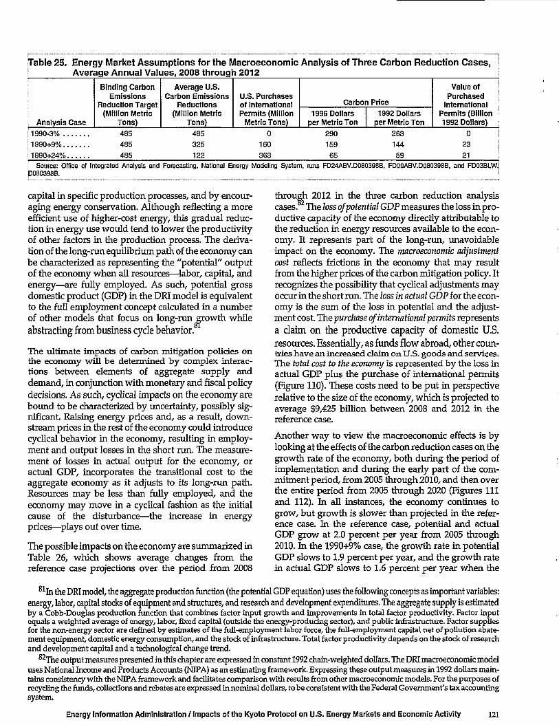
•
Table 25. Energy Market Assumptions for the Macroeconomic Analysis of Three Carbon Reduction Cases,Average Annual Values, 2008 through 2012
Analysis Case1990-3%1990+9%1990+24%
Binding CarbonEmissions
Reduction Target(Million Metric
Tons)485485485
Average U.S.Carbon Emissions
Reductions(Million Metric
Tons)485325122
U.S. Purchasesof InternationalPermits (Million
Metric Tons)0
160363
Carbon Price1996 Dollars
per Metric Ton29015965
1992 Dollarsper Metric Ton
26314459
Value ofPurchased
InternationalPermits (Billion1992 Dollars)
0
23
21
i Source: Office of Integrated Analysis and Forecasting, National Energy Modeling System, runs FD24ABV.D080398B, FD09ABV.D080398B, and FD03BLWJD080398B. I
capital in specific production processes, and by encour-aging energy conservation. Although reflecting a moreefficient use of higher-cost energy, this gradual reduc-tion in energy use would tend to lower the productivityof other factors in the production process. The deriva-tion of the long-run equilibrium path of the economy canbe characterized as representing the "potential" outputof the economy when all resources—labor, capital, andenergy—are fully employed. As such, potential grossdomestic product (GDP) in the DRI model is equivalentto the full employment concept calculated in a numberof other models that focus on long-run jjrowth whileabstracting from business cycle behavior.'si
The ultimate impacts of carbon mitigation policies onthe economy will be determined by complex interac-tions between elements of aggregate supply anddemand, in conjunction with monetary and fiscal policydecisions. As such, cyclical impacts on the economy arebound to be characterized by uncertainty, possibly sig-nificant. Raising energy prices and, as a result, down-stream prices in the rest of the economy could introducecyclical behavior in the economy, resulting in employ-ment and output losses in the short run. The measure-ment of losses in actual output for the economy, oractual GDP, incorporates the transitional cost to theaggregate economy as it adjusts to its long-run path.Resources may be less than fully employed, and theeconomy may move in a cyclical fashion as the initialcause of the disturbance—the increase in energyprices—plays out over time.
The possible impacts on the economy are summarized inTable 26, which shows average changes from thereference case projections over the period from 2008
through 2012 in the three carbon reduction analysiscases. The loss of potential GDP measures the loss in pro-ductive capacity of the economy directly attributable tothe reduction in energy resources available to the econ-omy. It represents part of the long-run, unavoidableimpact on the economy. The macroeconomic adjustmentcost reflects frictions in the economy that may resultfrom the higher prices of the carbon mitigation policy. Itrecognizes the possibility that cyclical adjustments mayoccur in the short run. The loss in actual GDP for the econ-omy is the sum of the loss in potential and the adjust-ment cost. The purchase of international permits representsa claim on the productive capacity of domestic U.S.resources. Essentially, as funds flow abroad, other coun-tries have an increased claim on U.S. goods and services.The total cost to the economy is represented by the loss inactual GDP plus the purchase of international permits(Figure 110). These costs need to be put in perspectiverelative to the size of the economy, which is projected toaverage $9,425 billion between 2008 and 2012 in thereference case.
Another way to view the macroeconomic effects is bylooking at the effects of the carbon reduction cases on thegrowth rate of the economy, both during the period ofimplementation and during the early part of the com-mitment period, from 2005 through 2010, and then overthe entire period from 2005 through 2020 (Figures 111and 112). In all instances, the economy continues togrow, but growth is slower than projected in the refer-ence case. In the reference case, potential and actualGDP grow at 2.0 percent per year from 2005 through2010. In the 1990+9% case, the growth rate in potentialGDP slows to 1.9 percent per year, and the growth ratein actual GDP slows to 1.6 percent per year when the
^In the DRI model, the aggregate production function (the potential GDP equation) uses the following concepts as important variables:energy, labor, capital stocks of equipment and structures, and research and development expenditures. The aggregate supply is estimatedby a Cobb-Douglas production function that combines factor input growth and improvements in total factor productivity. Factor inputequals a weighted average of energy, labor, fixed capital (outside the energy-producing sector), and public infrastructure. Factor suppliesfor the non-energy sector are defined by estimates of the full-employment labor force, the full-employment capital net of pollution abate-ment equipment, domestic energy consumption, and the stock of infrastructure. Total factor productivity depends on the stock of researchand development capital and a technological change trend.
82The output measures presented in this chapter are expressed in constant 1992 chain-weighted dollars. The DRI macroeconomic modeluses National Income and Products Accounts (NIPA) as an estimating framework. Expressing these output measures in 1992 dollars main-tains consistency with the NIPA framework and facilitates comparison with results from other macroeconomic models. For the purposes ofrecycling the funds, collections and rebates are expressed in nominal dollars, to be consistent with the Federal Government's tax accountingsystem.
Energy Information Administration / Impacts of the Kyoto Protocol on U.S. Energy Markets and Economic Activity 121
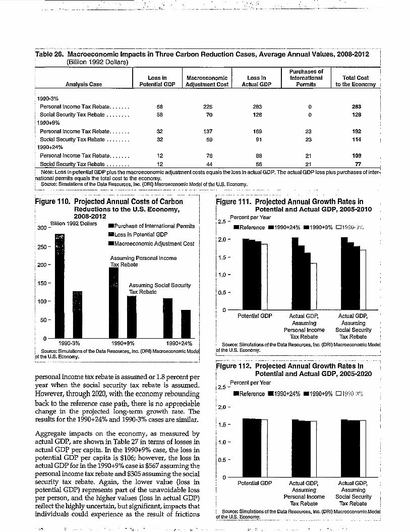
Table 26. Macroeconomic Impacts in Three Carbon Reduction Cases, Average Annual Values, 2008-2012(Billion 1992 Dollars)
Analysis CaseLoss in
Potential GDPMacroeconomicAdjustment Cost
Loss inActual GDP
Purchases ofInternational
PermitsTotal Cost
to the Economy
1990-3%
Personal Income Tax Rebate.
Social Security Tax Rebate . .
1990+9%
Personal Income Tax Rebate.
Social Security Tax Rebate . .
1990+24%
Personal Income Tax Rebate.
Social Security Tax Rebate . .
5858
32
32
12
12
225
70
137
59
76
44
283
128
169
91
8856
0
0
23
23
2121
283
128
192114
109
77
Note: Loss in potential GDP plus the macroeconomic adjustment costs equals the loss in actual GDP. The actual GDP loss plus purchases of inter-,'national permits equals the total cost to the economy.
Source: Simulations of the Data Resources, Inc. (DRI) Macroeconomic Model of the U.S. Economy.
Figure 110. Projected Annual Costs of CarbonReduct ions to the U.S. Economy,2008-2012
•Purchase of International Permits
•Loss in Potential GDP
•Macroeconomic Adjustment Cost
3 0 0 -Billion 1992 Dollars
2 5 0 -
2 0 0 -Assuming Personal IncomeTax Rebate
Assuming Social SecurityTax Rebate
1990-3% 1990+9% 1990+24%Source: Simulations of the Data Resources, Inc. (DRI) Macroeconomic Model
of the U.S. Economy.
personal income tax rebate is assumed or 1.8 percent peryear when the social security tax rebate is assumed.However, through 2020, with the economy reboundingback to the reference case path, there is no appreciablechange in the projected long-term growth rate. Theresults for the 1990+24% and 1990-3% cases are similar.
Aggregate impacts on the economy, as measured byactual GDP, are shown in Table 27 in terms of losses inactual GDP per capita. In the 1990+9% case, the loss inpotential GDP per capita is $106; however, the loss inactual GDP for in the 1990+9% case is $567 assuming thepersonal income tax rebate and $305 assuming the socialsecurity tax rebate. Again, the lower value (loss inpotential GDP) represents part of the unavoidable lossper person, and the higher values (loss in actual GDP)reflect the highly uncertain, but significant, impacts thatindividuals could experience as the result of frictions
Figure 111. Projected Annual Growth Rates inPotential and Actual GDP, 2005-2010
Potential GDP Actual GDP, Actual GDP,Assuming Assuming
Personal Income Social SecurityTax Rebate Tax Rebate ;
Source: Simulations of the Data Resources, Inc. (DRI) Macroeconomic Modelof the U.S. Economy. ,
2 . 5 -
2 . 0 -
Percent per Year
•Reference ^1990+24% ^1990+9% 01990-3%
Figure 112. Projected Annual Growth Rates inPotential and Actual GDP, 2005-2020
2 . 5 -Percent per Year
IReference • 1990+24% • 1990+9% • 1990-3%
2 . 0 -
1.5-
1.0-
0.5-
Potential GDP Actual GDP, Actual GDP, :Assuming Assuming j
Personal Income Social Security '•,Tax Rebate Tax Rebate I
) Source: Simulations of the Data Resources, Inc. (DRI) Macroeconomic Modelof the U.S. Economy. i
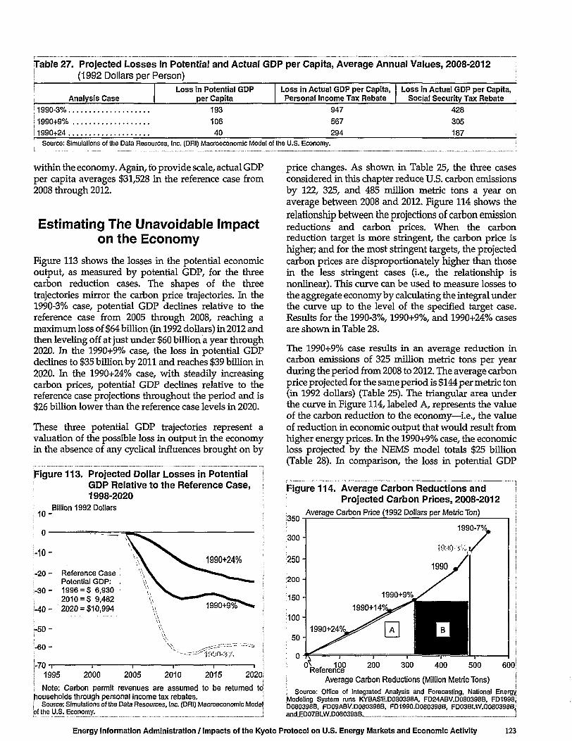
Table 27 Projected Losses in Potential and Actual(1992 Dollars per Person)
Analysis Case
1990-3%.
1990+9%
1990+24.
Loss in Potential GDPper Capita
193
106
40
GDP per Capita, Average Annual Values, 2008-2012
Loss in Actual GDP per Capita,Personal Income Tax Rebate
947
567
294
Loss in Actual GDP per Capita,Social Security Tax Rebate
428
305
187Source: Simulations of the Data Resources, Inc. (DRI) Macroeconomic Model of the U.S. Economy.
within the economy. Again, to provide scale, actual GDPper capita averages $31,528 in the reference case from2008 through 2012.
Estimating The Unavoidable Impacton the Economy
Figure 113 shows the losses in the potential economicoutput, as measured by potential GDP, for the threecarbon reduction cases. The shapes of the threetrajectories mirror the carbon price trajectories. In the1990-3% case, potential GDP declines relative to thereference case from 2005 through 2008, reaching amaximum loss of $64 billion (in 1992 dollars) in 2012 andthen leveling off at just under $60 billion a year through2020. In the 1990+9% case, the loss in potential GDPdeclines to $35 billion by 2011 and reaches $39 billion in2020. In the 1990+24% case, with steadily increasingcarbon prices, potential GDP declines relative to thereference case projections throughout the period and is$26 billion lower than the reference case levels in 2020.
These three potential GDP trajectories represent avaluation of the possible loss in output in the economyin the absence of any cyclical influences brought on by
figure 113, Projected Dollar Losses in PotentialGDP Relative to the Reference Case,1998-2020
10-
• 1 0 -
Billion 1992 Dollars
i-20 - Reference CasePotential GDP:
|-30 - 1996 = $ 6,9302010 = $ 9,482
j - 40 - 2020 = $10,994
I -50-i
i-60 -
V.
\
1990+9°/o
-70 T
1995 2000 2005 2010 2015 2020
Note: Carbon permit revenues are assumed to be returned tojhouseholds through personal income tax rebates.! Source: Simulations of the Data Resources, Inc. (DRI) Macroeconomic Modeljpf the U.S. Economy.
price changes. As shown in Table 25, the three casesconsidered in this chapter reduce U.S. carbon emissionsby 122, 325, and 485 million metric tons a year onaverage between 2008 and 2012. Figure 114 shows therelationship between the projections of carbon emissionreductions and carbon prices. When the carbonreduction target is more stringent, the carbon price ishigher; and for the most stringent targets, the projectedcarbon prices are disproportionately higher than thosein the less stringent cases (i.e., the relationship isnonlinear). This curve can be used to measure losses tothe aggregate economy by calculating the integral underthe curve up to the level of the specified target case.Results for the 1990-3%, 1990+9%, and 1990+24% casesare shown in Table 28.
The 1990+9% case results in an average reduction incarbon emissions of 325 million metric tons per yearduring the period from 2008 to 2012. The average carbonprice projected for the same period is $144 per metric ton(in 1992 dollars) (Table 25). The triangular area underthe curve in Figure 114, labeled A, represents the valueof the carbon reduction to the economy—i.e., the valueof reduction in economic output that would result fromhigher energy prices. In the 1990+9% case, the economicloss projected by the NEMS model totals $25 billion(Table 28). In comparison, the loss in potential GDP
Figure 114. Average Carbon Reductions and ;Projected Carbon Prices, 2008-2012 I
, Average Carbon Price (1992 Dollars per Metric Ton) i!350 ~~
0\ . 100 200 300 400 500 600Reference
Average Carbon Reductions (Million Metric Tons)Source: Office of Integrated Analysis and Forecasting, National Energy
Modeling System runs KYBASE.D080398A, FD24ABV.D080398B, FD1998*D080398B, FD09ABV.D080398B, FD1990.D080398B, FD03BLW.D080398B=and_ED07BLW.D080398B. I
Energy Information Administration / Impacts of the Kyoto Protocol on U.S. Energy Markets and Economic Activity 123

Table 28. Average Projected Annual Losses in Economic Output, 2008-2012
Analysis Case
Value of Lost Output
NENIS Valuation(Billion 1992 Dollars)
1990-3% 57
1990+9% 25
1990+24% 4
DRI Potential GDP Loss(Billion 1992 Dollars)
58
32
12
U.S. Purchase ofInternational Permits(Billion 1992 Dollars)
0
23
21Sources: Office of Integrated Analysis and Forecasting, National Energy Modeling System, runs FD24ABV.D080398B, FD09ABV.D080398B, and FD03BLW^
D080398B, and simulations of the Data Resources, Inc. (DRI) Macroeconomic Model of the U.S. Economy. I
Figure 115. Comparison of Average U.S. EconomicLosses Projected by the NEMS andDRI Models, 2008-2012
Potential Loss From Reference Case (Billion 1992 Dollars)80( 7 0 -
J s o -•40 -
J 3 0 -
|20-
ho-0
1990+24%
100 200 300 400 500 600
Average Carbon Reductions (Million Metric Tons)Source: Simulations of the Data Resources, Inc. (DRI) Macroeconomic Mode
bf the U.S. Economy.
calculated by the DRI model over the same period is $32billion. As a first approximation, this value closelymatches the estimate of the value of the lost outputcalculated independently using the energy modelresults (Figure 115).
The curve shown in Figure 114 can also be used toestimate the international value of traded permits. Thecarbon prices calculated in the NEMS model can becharacterized as the particular penalties that the UnitedStates would be willing to pay to achieve a given carbonmitigation target. For example, in the 1990+9% case, U.S.carbon emission reductions average 325 million metrictons per year during the period 2008 to 2012. Thedifference between that reduction and the binding target
of 485 million metric tons under the Kyoto Protocol (asreflected by the 1990-3% case) is assumed to be made upthrough purchases of international permits abroad. Thevalue of those purchases is shown as the rectangle Bunder the curve in Figure 114. For the 1990+9% case, thisrepresents a transfer of $23 billion dollars (1992 dollars)to purchase permits abroad. For the 1990+24% case, thetransfer is $21 billion (Table 25). Even though morepermits are purchased abroad, the purchases occurin the context of greater permit availability in the
1990+24% case, and the international price at which theyare bought is projected to be dramatically lower, asshown in Table 25.
Focusing on the last two columns of Table 28 highlightsthe role of international permit trading. Potential GDP isa measure of the level of the output of the economy, butas the last column indicates, there now is a cost to theeconomy reflected in the transfer of funds abroad to buypermits. Although the direct cost to the U.S. economy interms of lost potential GDP as a result of lower energyconsumption would be less in the 1990+24% and1990+9% cases than in the 1990-3% case, there would beadditional losses of output available to the U.S. economyin those cases. Funds transferred abroad for purchasesof international carbon emissions permits would, ineffect, reduce the amount of potential GDP available fordomestic use.
Energy Prices and the Role ofMonetary and Fiscal Policy
This following analysis focuses on the possible transi-tional impacts on the aggregate economy that wouldresult from efforts to reduce U.S. carbon emissions. Themeasurement of actual output for the economy, or actualGDP, is the key concept used in the examination ofchanges in the aggregate economy as it adjusts to itslong-run path. In addition to internal frictions caused bywage-price interactions and capital stock obsolescence,losses in domestic income may occur as funds are trans-ferred out of the United States to purchase internationalcarbon permits. Resources may be less than fullyemployed, and the economy will move in a cyclical fash-ion as the initial cause of the disturbance—the increase
in energy prices—plays out over time. Shifts in the secto-ral composition of the economy would also accompanythe adjustment process.
Here, a single fiscal policy is assumed to accompany thecarbon mitigation policy—the revenues collected fromthe domestic permit auction are returned to consumersthrough personal income tax rebates. This is a stylizedanalysis in that it represents only one of a wide range ofpossible combinations of monetary and fiscal responses.
124 Energy Information Administration / Impacts of the Kvoto Protocol on U.S. Enerav Markets anri Frnnnmin Af»tiuitu
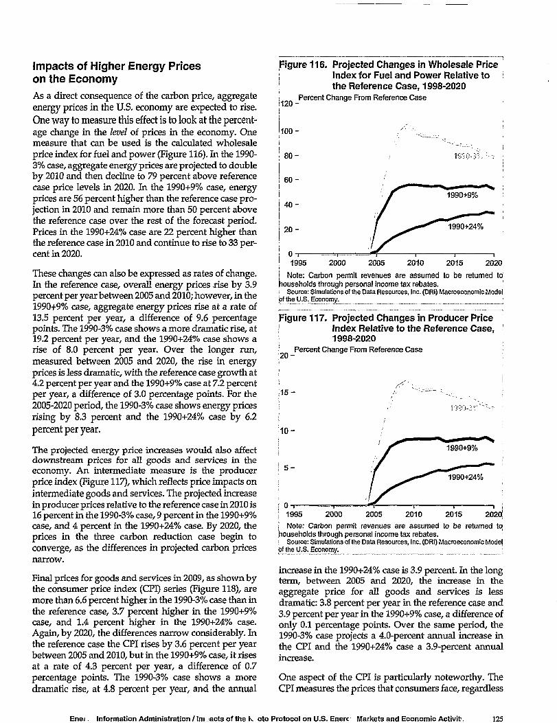
Impacts of Higher Energy Priceson the EconomyAs a direct consequence of the carbon price, aggregateenergy prices in the U.S. economy are expected to rise.One way to measure this effect is to look at the percent-age change in the level of prices in the economy. Onemeasure that can be used is the calculated wholesaleprice index for fuel and power (Figure 116). In the 1990-3% case, aggregate energy prices are projected to doubleby 2010 and then decline to 79 percent above referencecase price levels in 2020. In the 1990+9% case, energyprices are 56 percent higher than the reference case pro-jection in 2010 and remain more than 50 percent abovethe reference case over the rest of the forecast period.Prices in the 1990+24% case are 22 percent higher thanthe reference case in 2010 and continue to rise to 33 per-cent in 2020.
These changes can also be expressed as rates of change.In the reference case, overall energy prices rise by 3.9percent per year between 2005 and 2010; however, in the1990+9% case, aggregate energy prices rise at a rate of13.5 percent per year, a difference of 9.6 percentagepoints. The 1990-3% case shows a more dramatic rise, at19.2 percent per year, and the 1990+24% case shows arise of 8.0 percent per year. Over the longer run,measured between 2005 and 2020, the rise in energyprices is less dramatic, with the reference case growth at4.2 percent per year and the 1990+9% case at 7.2 percentper year, a difference of 3.0 percentage points. For the2005-2020 period, the 1990-3% case shows energy pricesrising by 8.3 percent and the 1990+24% case by 6.2percent per year.
The projected energy price increases would also affectdownstream prices for all goods and services in theeconomy. An intermediate measure is the producerprice index (Figure 117), which reflects price impacts onintermediate goods and services. The projected increasein producer prices relative to the reference case in 2010 is16 percent in the 1990-3% case, 9 percent in the 1990+9%case, and 4 percent in the 1990+24% case. By 2020, theprices in the three carbon reduction case begin toconverge, as the differences in projected carbon pricesnarrow.
Final prices for goods and services in 2009, as shown bythe consumer price index (CPI) series (Figure 118), aremore than 6.6 percent higher in the 1990-3% case than inthe reference case, 3.7 percent higher in the 1990+9%case, and 1.4 percent higher in the 1990+24% case.Again, by 2020, the differences narrow considerably. Inthe reference case the CPI rises by 3.6 percent per yearbetween 2005 and 2010, but in the 1990+9% case, it risesat a rate of 4.3 percent per year, a difference of 0.7percentage points. The 1990-3% case shows a moredramatic rise, at 4.8 percent per year, and the annual
Figure 116. Projected Changes in Wholesale Price; Index for Fuel and Power Relative to
the Reference Case, 1998-2020
120-
100-
8 0 -
6 0 -
4 0 -
2 0 -
Percent Change From Reference Case
1990-3^ ; -
O n —1995
1990+24%
2000 2005 2010 2015 2020
Note: Carbon permit revenues are assumed to be returned to!iouseholds through personal income tax rebates.
Source: Simulations of the Data Resources, Inc. (DRI) Macroeconomio Mode)af the U.S. Economy.
Figure 117. Projected Changes in Producer Pricei Index Relative to the Reference Case,I 1998-2020
2 0 -
1 5 -
10-
5 -
Percent Change From Reference Case
! 990-3';:
1990+24%
1995 2000 2005 2010 2015 2020,Note: Carbon permit revenues are assumed to be returned tq
households through personal income tax rebates.| Source: Simulations of the Data Resources, Inc. (DRI) Macroeconomic Mode|bf the U.S. Economy. ;
increase in the 1990+24% case is 3.9 percent. In the longterm, between 2005 and 2020, the increase in theaggregate price for all goods and services is lessdramatic: 3.8 percent per year in the reference case and3.9 percent per year in the 1990+9% case, a difference ofonly 0.1 percentage points. Over the same period, the1990-3% case projects a 4.0-percent annual increase inthe CPI and the 1990+24% case a 3.9-percent annualincrease.
One aspect of the CPI is particularly noteworthy. TheCPI measures the prices that consumers face, regardless
Enei. Information Administration / Im acts of the K oto Protocol on U.S. Enerc Markets and Economic Activit 125
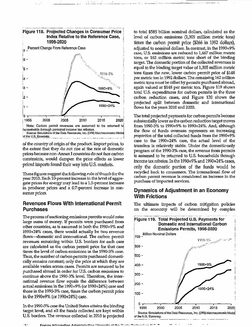
Figure 118. Projected Changes in Consumer PriceI Index Relative to the Reference Case,
1998-2020
7 -
6 -
5 -
; 4 -
3 -
2 -
1 -
Percent Change From Reference Case
1995 2000 2005 2010 2015 2020J
Note: Carbon permit revenues are assumed to be returned tohouseholds through personal income tax rebates. j! Source: Simulations of the Data Resources, Inc. (DRI) Macroeconomic Modelof the U.S. Economy. j
of the country of origin of the product. Import prices, tothe extent that they do not rise at the rate of domesticprices because non-Annex I countries do not face carbonconstraints, would dampen the price effects as lowerpriced imports found their way into U.S. markets.
These figures suggest the following rule of thumb for theyear 2010. Each 10-percent increase in the level of aggre-gate prices for energy may lead to a 1.5-percent increasein producer prices and a 0.7-percent increase in con-sumer prices.
Revenues Flows With International PermitPurchases
The process of auctioning emissions permits would raiselarge sums of money. If permits were purchased fromother countries, as is assumed in both the 1990+9% and1990+24% cases, there would actually be two revenueflows—domestic and international. The carbon permitrevenues remaining within U.S. borders for each caseare calculated as the carbon permit price for that casetimes the level of carbon emissions in the 1990-3% case.Thus, the number of carbon permits purchased domesti-cally remains constant; only the price at which they areavailable varies across cases. Permits are assumed to bepurchased abroad in order for U.S. carbon emissions tocontinue above the 1990-3% level. Therefore, the inter-national revenue flow equals the difference betweenactual emissions in the 1990+9% (or 1990+24%) case andthose in the 1990-3% case, times the carbon permit pricein the 1990+9% (or 1990+24%) case.
In the 1990-3% case the United States attains the bindingtarget level, and all the funds collected are kept withinU.S. borders. The revenue collected in 2010 is projected
to total $585 billion nominal dollars, calculated as thelevel of carbon emissions (1,305 million metric tons)times the carbon permit price ($266 in 1992 dollars),adjusted to nominal dollars. In contrast, in the 1990+9%case, U.S. emissions are reduced to 1,467 million metrictons, or 162 million metric tons short of the bindingtarget. The domestic portion of the collected revenues isequal to the binding target value of 1,305 million metrictons times the new, lower carbon permit price of $148per metric ton in 1992 dollars. The remaining 162 millionmetric tons must be offset by permits purchased abroad,again valued at $148 per metric ton. Figure 119 showstotal U.S. expenditures for carbon permits in the threecarbon reduction cases, and Figure 120 shows theprojected split between domestic and internationalflows for the years 2010 and 2020.
The total projected payments for carbon permits becomesubstantially lower as the carbon reduction target movesfrom 1990-3% to 1990+9% to 1990+24%. And, althoughthe flow of funds overseas represents an increasingproportion of the total collected funds from the 1990+9%case to the 1990+24% case, the actual level of thetransfers is relatively stable. Under the domestic-onlyprogram of the 1990-3% case, the revenue from permitsis assumed to be returned to U.S. households throughincome tax rebates. In the 1990+9% and 1990+24% cases,only the domestic portion of the funds would berecycled back to consumers. The international flow ofcarbon permit revenue is considered an increase in thepurchase of imported services.
Dynamics of Adjustment in an EconomyWith Frictions
The ultimate impacts of carbon mitigation policieson the economy will be determined by complex
Figure 119. Total Projected U.S. Payments for| Domestic and International Carbon| Emissions Permits, 1998-2020
7 0 0 -
6 0 0 -
J500-
J400-
3 0 0 -
2 0 0 -
100-
Billion Nominal Dollars
1990-3%
1990+24%
1995 2000 2005 2010 2015 2020)Source: Simulations of the Data Resources, Inc. (DRI) Macroeconomic Mode(
of the U.S. Economy.
Pnprnv lnfnr

Figure 120. Projected Destinations of Funds Paid! for Carbon Emissions Permits, 2010! and 2020j Billion Nominal Dollars
•International Payments
700 - •Domestic Payments 1990-3%
i 6 0 0 _ 1990-3%
2010 2020
Source: Simulations of the Data Resources, Inc. (DRI) Macroeconomic Modelpf the U.S. Economy.
interactions between elements of aggregate supply anddemand, in conjunction with monetary and fiscal policydecisions. As such, any discussion of possible cyclicalimpacts on the economy is bound to be characterized byuncertainty and controversy. It should be recognized,however, that the process of raising the price of energyand downstream prices in the rest of the economy by themagnitudes shown in Figure 116, 117, and 118 couldintroduce cyclical behavior in the economy resulting inemployment and output losses beyond those associatedwith the projected impacts on potential GDP.
The introduction of carbon emission limits would affectboth consumers and businesses. Households would befaced with higher prices for energy and the need toadjust spending patterns. Nominal energy expenditureswould rise, taking a larger share of the family budget forgoods and service consumption and leaving less for sav-ings. Higher prices for energy would cause consumersto try to reduce spending not only on energy, but onother goods as well. Thus, changes in energy priceswould tend to disrupt both saving and spendingstreams.
Energy services also represent a key input in the produc-tion of goods and services. As energy prices increase, thecosts of production rise, placing upward pressure on thenominal prices of all intermediate goods and final goodsand services in the economy, with widespread impactson spending across many markets. The ultimate effectwill depend on opportunities for substitution away fromhigher-cost energy to other goods and services and theeffectiveness of compensatory fiscal and monetarypolicy.
The transitional adjustment of the economy can be cap-tured by calculations of the actual GDP of the economy.The impacts on actual GDP represent a measure of theloss of output from the economy, recognizing thatadjustments are not frictionless and that all resourcesmay not be fully employed in the near term. The outputof the economy as reflected by actual GDP can cyclearound the measure of potential GDP.
The Role of Monetary PolicyMonetary policy can moderate or intensify the ultimateimpacts on the economy; however, trying to predict theresponse of monetary authorities to large increases inenergy prices is a difficult task. The emphasis on control-ling inflation relative to concerns about rising unem-ployment has changed over the past 20 years, and usinghistory as a guide does not remove the large amount ofuncertainty about the response of monetary authorities.In addition, the types of financial instruments availablehave become more numerous and more interdependent,and the task of monitoring the Nation's money supplyhas become more complex.
The monetary authorities could concentrate on in-creased inflation resulting from higher energy pricesand choose not to increase the money supply in order tomoderate the resulting inflation. In this instance, outputand employment losses would be larger than theywould if the money supply were expanded when energyprices increased. Another option would be to allow themoney supply to increase in order to remove the unem-ployment impacts while allowing substantial additionalprice inflation. This analysis uses neither extreme ofthese assumptions about the response of the FederalReserve. The discussion that follows represents a middlepath that the Federal Reserve might follow.
In the setting that has been described—returning fundsin the form of personal income tax rebates—higherprices in the economy would place upward pressure oninterest rates. The Federal Reserve Board would thenseek to balance the consequences of higher energy priceson the economy with possible adverse effects on outputand employment. The Federal Reserve would respondto changes in inflation and unemployment brought onby the initial carbon mitigation policy by making adjust-ments to influence the Federal funds rate.83 The adjust-ments would be designed to moderate the possibleimpacts on both inflation and unemployment, and toreturn the economy toward its long-run growth path.The characterization of monetary policy reactions toinflation and unemployment used in these simulationsis based on a DRI reaction function that has been esti-mated to reflect the historical relationship between the
83The Federal funds rate is the rate charged by a depository institution on an overnight sale of Federal funds to another depository insti-tution. This rate influences the trend in behavior for other interest rates in the economy.
Energy Information Administration / Impacts of the Kyoto Protocol on U.S. Energy Markets and Economic Activity 127
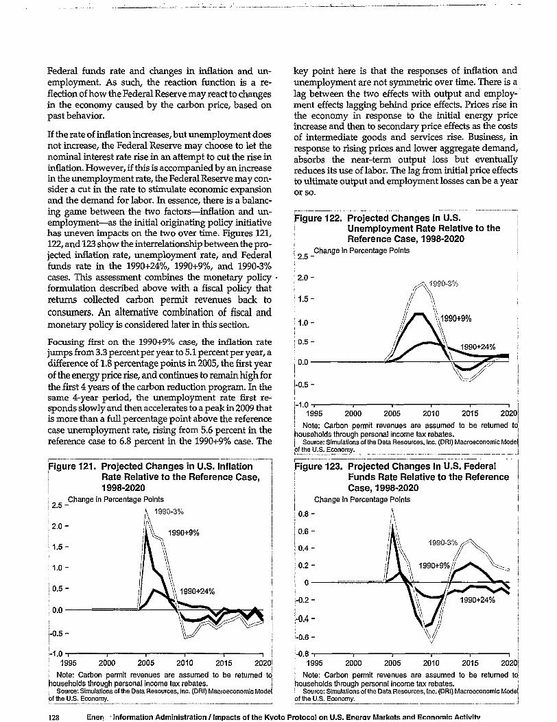
Federal funds rate and changes in inflation and un-employment. As such, the reaction function is a re-flection of how the Federal Reserve may react to changesin the economy caused by the carbon price, based onpast behavior.
If the rate of inflation increases, but unemployment doesnot increase, the Federal Reserve may choose to let thenominal interest rate rise in an attempt to cut the rise ininflation. However, if this is accompanied by an increasein the unemployment rate, the Federal Reserve may con-sider a cut in the rate to stimulate economic expansionand the demand for labor. In essence, there is a balanc-ing game between the two factors—inflation and un-employment—as the initial originating policy initiativehas uneven impacts on the two over time. Figures 121,122, and 123 show the interrelationship between the pro-jected inflation rate, unemployment rate, and Federalfunds rate in the 1990+24%, 1990+9%, and 1990-3%cases. This assessment combines the monetary policyformulation described above with a fiscal policy thatreturns collected carbon permit revenues back toconsumers. An alternative combination of fiscal andmonetary policy is considered later in this section.
Focusing first on the 1990+9% case, the inflation ratejumps from 3.3 percent per year to 5.1 percent per year, adifference of 1.8 percentage points in 2005, the first yearof the energy price rise, and continues to remain high forthe first 4 years of the carbon reduction program. In thesame 4-year period, the unemployment rate first re-sponds slowly and then accelerates to a peak in 2009 thatis more than a full percentage point above the referencecase unemployment rate, rising from 5.6 percent in thereference case to 6.8 percent in the 1990+9% case. The
Figure 121. Projected Changes in U.S. InflationRate Relative to the Reference Case,1998-2020
2 . 5 -
2 . 0 -
1.5-
1.0-
0 .5 -
0.0 —
- 0 . 5 -
Change in Percentage Points
1990-3%
1990+9%
1-1.0 •1995 2000 2005 2010 2015 2020!
Note: Carbon permit revenues are assumed to be returned tohouseholds through personal income tax rebates. I
Source: Simulations of the Data Resources, Inc. (DRI) Macroeconomic Mode(bf the U.S. Economy. I
key point here is that the responses of inflation andunemployment are not symmetric over time. There is alag between the two effects with output and employ-ment effects lagging behind price effects. Prices rise inthe economy in response to the initial energy priceincrease and then to secondary price effects as the costsof intermediate goods and services rise. Business, inresponse to rising prices and lower aggregate demand,absorbs the near-term output loss but eventuallyreduces its use of labor. The lag from initial price effectsto ultimate output and employment losses can be a year
or so.
Figure 122. Projected Changes in U.S.I Unemployment Rate Relative to the
Reference Case, 1998-2020
2 . 5 -Change in Percentage Points
1995 2000 2005 2010 2015 2020
Note: Carbon permit revenues are assumed to be returned tohouseholds through personal income tax rebates. i
Source: Simulations of the Data Resources, Inc. (DRI) Macroeconomic Modelof the U.S. Economy. i
Figure 123. Projected Changes in U.S. FederalFunds Rate Relative to the ReferenceCase, 1998-2020
Change in Percentage Points
0 . 8 -
i-0.8 •1995 2000 2005 2010 2015 2020
Note: Carbon permit revenues are assumed to be returned tohouseholds through personal income tax rebates. ji Source: Simulations of the Data Resources, Inc. (DRI) Macroeconomic Modelbf the U.S. Economy.
128 Enen • Information Administration / Impacts of the Kvoto Protocol on U.S. Enerav Markets and Economic Activity
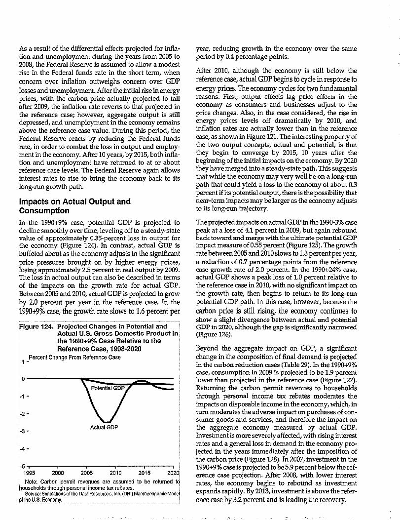
As a result of the differential effects projected for infla-tion and unemployment during the years from 2005 to2008, the Federal Reserve is assumed to allow a modestrise in the Federal funds rate in the short term, whenconcern over inflation outweighs concern over GDPlosses and unemployment. After the initial rise in energyprices, with the carbon price actually projected to fallafter 2009, the inflation rate reverts to that projected inthe reference case; however, aggregate output is stilldepressed, and unemployment in the economy remainsabove the reference case value. During this period, theFederal Reserve reacts by reducing the Federal fundsrate, in order to combat the loss in output and employ-ment in the economy. After 10 years, by 2015, both infla-tion and unemployment have returned to at or aboutreference case levels. The Federal Reserve again allowsinterest rates to rise to bring the economy back to itslong-run growth path.
Impacts on Actual Output andConsumptionIn the 1990+9% case, potential GDP is projected todecline smoothly over time, leveling off to a steady-statevalue of approximately 0.35-percent loss in output forthe economy (Figure 124). In contrast, actual GDP isbuffeted about as the economy adjusts to the significantprice pressures brought on by higher energy prices,losing approximately 2.5 percent in real output by 2009.The loss in actual output can also be described in termsof the impacts on the growth rate for actual GDP.Between 2005 and 2010, actual GDP is projected to growby 2.0 percent per year in the reference case. In the1990+9% case, the growth rate slows to 1.6 percent per
igure 124. Projected Changes in Potential andActual U.S. Gross Domestic Product inthe 1990+9% Case Relative to theReference Case, 1998-2020
1 -Percent Change From Reference Case
-1 -
- 3 -
i-4-
Actual GDP
i-5-1995 2000 2005 2010 2015 2020
J Note: Carbon permit revenues are assumed to be returned tohouseholds through personal income tax rebates.
Source: Simulations of the Data Resources, Inc. (DRI) Macroeconomic Modejof the U.S. Economy.
year, reducing growth in the economy over the sameperiod by 0.4 percentage points.
After 2010, although the economy is still below thereference case, actual GDP begins to cycle in response toenergy prices. The economy cycles for two fundamentalreasons. First, output effects lag price effects in theeconomy as consumers and businesses adjust to theprice changes. Also, in the case considered, the rise inenergy prices levels off dramatically by 2010, andinflation rates are actually lower than in the referencecase, as shown in Figure 121. The interesting property ofthe two output concepts, actual and potential, is thatthey begin to converge by 2015, 10 years after thebeginning of the initial impacts on the economy. By 2020they have merged into a steady-state path. This suggeststhat while the economy may very well be on a long-runpath that could yield a loss to the economy of about 0.3percent if its potential output, there is the possibility thatnear-term impacts maybe larger as the economy adjuststo its long-run trajectory.
The projected impacts on actual GDP in the 1990-3% casepeak at a loss of 4.1 percent in 2009, but again reboundback toward and merge with the ultimate potential GDPimpact measure of 0.55 percent (Figure 125). The growthrate between 2005 and 2010 slows to 1.3 percent per year,a reduction of 0.7 percentage points from the referencecase growth rate of 2.0 percent. In the 1990+24% case,actual GDP shows a peak loss of 1.0 percent relative tothe reference case in 2010, with no significant impact onthe growth rate, then begins to return to its long-runpotential GDP path. In this case, however, because thecarbon price is still rising, the economy continues toshow a slight divergence between actual and potentialGDP in 2020, although the gap is significantly narrowed(Figure 126).
Beyond the aggregate impact on GDP, a significantchange in the composition of final demand is projectedin the carbon reduction cases (Table 29). In the 1990+9%case, consumption in 2009 is projected to be 1.9 percentlower than projected in the reference case (Figure 127).Returning the carbon permit revenues to householdsthrough personal income tax rebates moderates theimpacts on disposable income in the economy, which, inturn moderates the adverse impact on purchases of con-sumer goods and services, and therefore the impact onthe aggregate economy measured by actual GDP.Investment is more severely affected, with rising interestrates and a general loss in demand in the economy pro-jected in the years immediately after the imposition ofthe carbon price (Figure 128). In 2007, investment in the1990+9% case is projected to be 5.9 percent below the ref-erence case projection. After 2008, with lower interestrates, the economy begins to rebound as investmentexpands rapidly. By 2013, investment is above the refer-ence case by 3.2 percent and is leading the recovery.

Figure 125. Projected Changes in Potential and[ Actual U.S. Gross Domestic Product in! the 1990-3% Case Relative to the
Reference Case, 1998-2020
1 -Percent Change From Reference Case
[ - 1 -
jj - 2 -
ji - 4 -
Actual GDP
!-51995 2000 2005 2010 2015 2020
Note: Carbon permit revenues are assumed to be returned tohouseholds through personal income tax rebates. ;j Source: Simulations of the Data Resources, Inc. (DRl) Macroeconomic Modelof the U.S. Economy. •
Figure 126. Projected Changes in Potential and: Actual U.S. Gross Domestic Product in! the 1990+24% Case Relative to theI Reference Case, 1998-2020
Percent Change From Reference Case
-1 -
- 2 -
• - 3 -
Potential GDP
s ^Actual GDP
-5-1995 2000 2005 2010 2015 2020
| Note: Carbon permit revenues are assumed to be returned tohouseholds through personal income tax rebates.j Source: Simulations of the Data Resources, Inc. (DRl) Macroeconomic Modelof the U.S. Economy. I
The 1990-3% case shows a pattern of adjustment similarto that projected in the 1990+9% case, except that thereaction in terms of both consumption and investment ismore extreme, given the higher carbon price. Consump-tion reaches its lowest point in the year 2009 at 2.8percent below the reference case. Thereafter, consump-tion returns to the reference case level in 2013 and by2015 is 0.8 percent above the reference case level.Investment is more volatile, falling to 9.1 percent belowreference case levels by 2008. Again, with interest rates
Figure 127. Projected Changes in RealConsumption in the U.S. EconomyRelative to the Reference Case,1998-2020
Percent Change From Reference Case
1990+9%
-101995 2000 2005 2010 2015 2020
: Note: Carbon permit revenues are assumed to be returned tojJiouseholds through personal income tax rebates. <
Source: Simulations of the Data Resources, Inc. (DRl) Macroeconomic Modejof the U.S. Economy. !
Figure 128. Projected Changes in RealInvestment in the U.S. EconomyRelative to the Reference Case,1998-2020
Percent Change From Reference Case
1995 2000 2005 2010 2015 2020
Note: Carbon permit revenues are assumed to be returned tohouseholds through personal income tax rebates.i Source: Simulations of the Data Resources, Inc. (DRl) Macroeconomic Modelof the U.S. Economy. i
declining relative to the reference case after 2010, invest-ment recovers rapidly and by 2013 is 5.1 percent abovethe reference case.
The 1990+24% case reflects a much smoother path forboth consumption and investment. Consumption re-mains below the reference case throughout the period,but with a maximum loss of only 0.8 percent in 2010. Theimpact on investment, likewise, is more moderate thanin the 1990-3% and 1990+9% cases, falling to 2.2 percent

Table 29. Projected Economic Impacts of Carbon Reduction Cases Assuming Personal Income Tax Rebate] (Changes From Reference Case)
Analysis Case 1 2010 2015 2020
1990-3%
Collections (Billion Nominal Dollars)
Wholesale Price Index for Fuel and Power (Percent Change).
Producer Price Index (Percent Change)
Consumer Price Index (Percent Change)
! Unemployment Rate (Difference in Rate)
j Federal Funds Rate (Difference in Rate)
! Potential GDP (Percent Change)
j Real GDP (Percent Change)
j Real GDP (Billion 1992 Chain-Weighted Dollars)
i Consumption (Percent Change)j Investment (Percent Change)
S Industrial Output (Percent Change)
1990+9%
Collections (Billion Nominal Dollars)
Wholesale Price Index for Fuel and Power (Percent Change).
Producer Price Index (Percent Change)
Consumer Price Index (Percent Change)
Unemployment Rate (Difference in Rate)
Federal Funds Rate (Difference in Rate)
Potential GDP (Percent Change)Real GDP (Percent Change)
Real GDP (Billion 1992 Chain-Weighted Dollars)
Consumption (Percent Change)
Investment (Percent Change)
Industrial Output (Percent Change)
1990+24%
Collections (Billion Nominal Dollars)
Wholesale Price Index for Fuel and Power (Percent Change).
Producer Price Index (Percent Change)
Consumer Price Index (Percent Change)
Unemployment Rate (Difference in Rate)
| Federal Funds Rate (Difference in Rate)Potential GDP (Percent Change)Real GDP (Percent Change)Real GDP (Billion 1992 Chain-Weighted Dollars)Consumption (Percent Change)
Investment (Percent Change)Industrial Output (Percent Change)
585
99.1
15.7
6.0
1.6
-0.7
-1.2
-3.5
-327
-2.3-3.6-5.8
317
55.7
9.03.5
0.9
-0.4-0.7-2.0-187
-1.5
-1.5-3.0
128
21.5
3.6
1.5
0.5-0.2-0.2
-1.0
-96
-0.8
-1.8-1.3
633
89.9
14.6
4.2
-0.4
0.5
-0.8
-0.1
-12
0.83.3-2.5
34053.78.82.5-0.20.2-0.4-0.1-150.21.8-1.6
206
29.3
4.9
1.6
0.2
-0.0-0.3-0.5-54-0.4
0.2
-1.3
674
78.9
12.9
2.9
0.1
0.1
-0.6
-0.7
-72
0.4-0.0-3.6
39152.58.72.10.2-0.1-0.4-0.6-68-0.2-0.1-3.1
271
32.9
5.5
1.4
0.1-0.1-0.3
-0.5
-49
-0.3
0.1-2.0
Source: Simulations of the Data Resources, Inc. (DRI) Macroeconomic Model of the U.S. Economy.
below the reference case in 2008. Thereafter, investmentreturns to the reference case level and essentially re-mains at that position for the remainder of the forecastperiod.
Figure 129 shows the projected impacts on consumptionand investment in terms of growth rates between 2005and 2010 and between 2005 and 2020. Between 2005 and2010, consumption growth rates fall from 2.0 percent peryear in the reference case to 1.9 percent in the 1990+24%case, 1.7 percent in the 1990+9% case, and 1.6 percent inthe 1990-3% case. Investment shows a similar, but morepronounced profile, with growth declining from 2.9percent per year in the reference case to 2.5 percent, 2.6
percent, and 2.2 percent in the respective carbonreduction cases. Slight variations in the order of theimpacts—the 1990+24% case at 2.5 percent and the1990+9% case at 2.6 percent—can be explained by thehighly cyclical effects on investment, as shown in Figure128. In the long run, as indicated by the projected growthrates between 2005 and 2020, growth in both con-sumption and investment returns to the reference caserates.
These results indicate that, as a result of higher energyprices, the economy may absorb a near-term loss in out-put in response to higher inflation and a rise in theunemployment rate. However* with appropriate action
Energy Information Administration / Impacts of the Kyoto Protocol on U.S. Enerav Markets and Ecnnnmip

Figure 129. Consumption and InvestmentGrowth Rates
Percent per Year
•Reference •1990+24% •1990+9% • 1990-3%
Note: Carbon permit revenues are assumed to be returned tohouseholds through personal income tax rebates. •| Source: Simulations of the Data Resources, inc. (DRI) Macroeconomic Modelof the U.S. Economy. J
on the part of the monetary authorities, these impactscould be mitigated, and in the long-term the economycould rebound.
The Role of Fiscal Policy
This analysis assumes that revenues from carbon per-mits would be collected by the Federal Government,which would have a number of alternatives with regardto their disposition. The producers of carbon-intensivefuels could keep the permit revenues; or the Govern-ment could either use the revenues to reduce thenational debt, return them to businesses through reduc-tions in corporate income tax rates or increased businesstax credits, return them to consumers through personalincome tax rebates, or return them to both consumersand businesses through social security tax rebates. Eachmethod of using the collected permit revenue isplausible, and each method would have a differenteconomic impact.
Returning the funds to consumers through personalincome tax rebates or returning them to consumers andbusinesses through social security tax rebates wouldwork to ameliorate the short-term impacts on the econ-omy by bolstering disposable income. Alternative fiscalpolicies, such as having the Federal Government use thefunds to lower the Federal debt level, or a corporateincome tax rebate, probably would result in larger
near-term impacts, because disposable income andtherefore consumption would fall by greater amounts.Conversely, policies that serve to shift the economyaway from consumption toward investment may havegreater long-term benefits in terms of expansion of theaggregate capital stock.
All the projections discussed so far in this chapter haveassumed a policy of returning carbon permit revenues tohouseholds through personal income tax rebates, usinga lump sum transfer. To highlight the potential signifi-cance of an alternative fiscal regime this chapter nextreviews the potential effects of a rebate of social securitytaxes that passes funds back to both employees andemployers in equal amounts. The analysis of a hypo-thetical rebate of the social security tax is meant only tobe descriptive of a tax measure that could have the effectof reducing price pressures in the economy by loweringbusiness costs, while also accomplishing a partial com-pensation to consumers for the higher energy bills theywould face. The two policies considered in this analy-sis—the personal income tax rebate and the social secu-rity tax rebate—are only meant to be representative of aset of possible fiscal policies that might accompany aninitial carbon mitigation policy.
The fundamental difference between the two policies isin their treatment of business. On the employer side, thereduction in employer contributions to the social secu-rity system would lower costs to the firm and, thereby,moderate the near-term price consequences to the econ-omy. Since it is the price effect that produces the pre-dominately negative effect on the economy, any steps toreduce inflationary pressures would serve to moderateadverse impacts on the economy. The smaller impact onaggregate prices would also moderate the monetary pol-icy reaction, as shown in Figures 130,131, and 132. In allthe carbon reduction cases, the reaction of the Federalfunds rate to the economic effects of higher energyprices would be less pronounced than projected underthe assumption of a personal income tax reduction.Similarly, the social security tax option would moderatethe potential impact on actual GDP in the carbon reduc-tion cases (Figure 133), largely because of the cost-cutting aspects of lowering of the employer portion ofthe tax. Similar moderating effects would be seen forconsumption (Figure 134) and investment (Figure 135).Under both policies, the economy would eventuallyrevert to a long-run path consistent with the path ofpotential output.
^In the DRI model for personal taxes only, a lump sum transfer produces the same effects as a cut in the personal income tax rate.
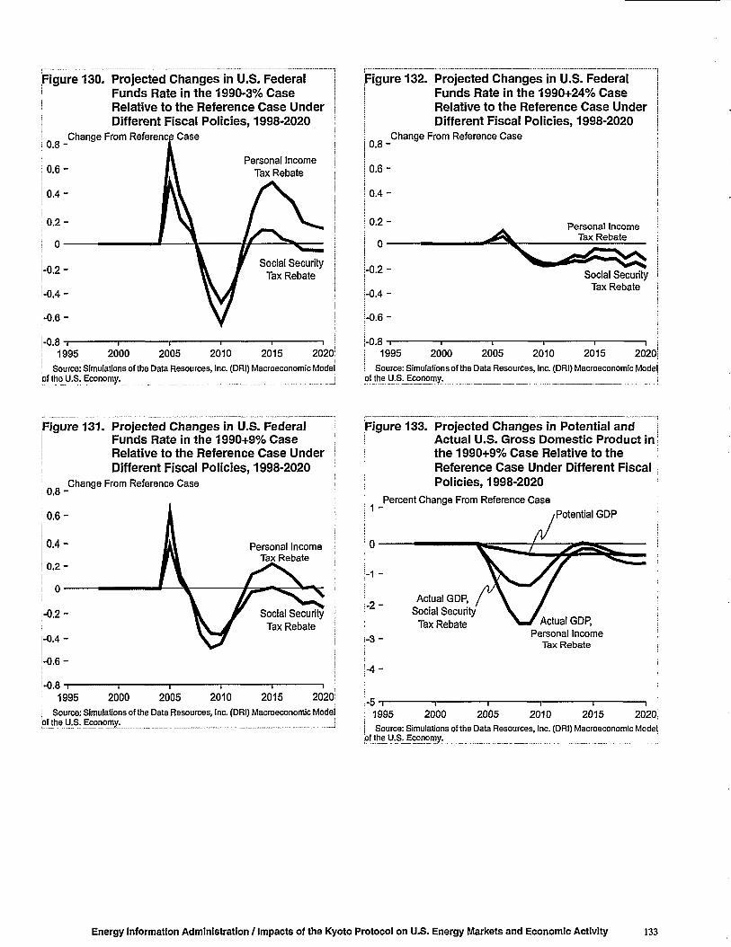
Figure 130. Projected Changes in U.S. Federal' Funds Rate in the 1990-3% CaseI Relative to the Reference Case Under| Different Fiscal Policies, 1998-2020
0 .8 -
0 .6 -
0 .4 -
0 .2 -
0 —
Change From Reference Case
Personal IncomeTax Rebate
-0 .2 -
-0 .4 -
-0 .6 -
Social SecurityTax Rebate
-0.8'1995 2000 2005 2010 2015 2020:
Source: Simulations of the Data Resources, Inc. (DRI) Macroeconomic Modelof the U.S. Economy.
Figure 132. Projected Changes in U.S. FederalFunds Rate in the 1990+24% CaseRelative to the Reference Case UnderDifferent Fiscal Policies, 1998-2020
0 .8 -
0 .6 -
0 .4 -
0 .2 -
Change From Reference Case
Personal IncomeTax Rebate
1995 2000 2005 2010 2015 2020|
Source: Simulations of the Data Resources, Inc. (DRI) Macroeconomic Modejof the U.S. Economy.
Figure 131. Projected Changes in U.S. FederalFunds Rate in the 1990+9% CaseRelative to the Reference Case UnderDifferent Fiscal Policies, 1998-2020
0 .8 -Change From Reference Case
Personal IncomeTax Rebate
2005 2010 2015 2020!Source: Simulations of the Data Resources, Inc. (DRI) Macroeconomic Model
of the U.S. Economy. __j
Figure 133. Projected Changes in Potential andActual U.S. Gross Domestic Product inthe 1990+9% Case Relative to theReference Case Under Different FiscalPolicies, 1998-2020
Percent Change From Reference Case
-1 -
- 2 -
- 3 -
- 4 -
-5-1—1995
Potential GDP
Actual GDP,Social Security'
Tax Rebate Actual GDP,Personal Income
Tax Rebate
2000 2005 2010 2015 2020.Source: Simulations of the Data Resources, Inc. (DRI) Macroeconomic Model
Of the U.S. Economy.
Energy Information Administration / Impacts of the Kyoto Protocol on U.S. Energy Markets and Economic Activity 133

Figure 134. Projected Changes in RealConsumption in the U.S. EconomyRelative to the Reference Case,1998-2020, Assuming a Social SecurityTax Rebate
6 -
4 -
2 -
0 -
Percent Change From Reference Case
1990-3%
-2-
-4-
-6-
-8-
1990+24%
1990+9%
.10-, , , , ,1995 2000 2005 2010 2015 2020Source: Simulations of the Data Resources, Inc. (DRI) Macroeconomic Model
of the U.S. Economy.
:igure 135. Projected Changes in RealInvestment in the U.S. EconomyRelative to the Reference Case,1998-2020, Assuming a Social SecurityTax Rebate
Percent Change From Reference Case
1990+9%
10 T 1 1 , \ 1
1995 2000 2005 2010 2015 2020Source: Simulations of the Data Resources, Inc. (DRI) Macroeconomic Model
iof the U.S. Economy. i
Energy Investment
This macroeconomic analysis of the costs of the KyotoProtocol includes the direct fuel costs and only thoseinvestment costs that are comparable in magnitude withthose in the reference case. Business investments abovereference case levels may be required to reduce energycosts in response to increasing energy prices. The poten-tial incremental costs of investment in technology andinfrastructure that may be necessary to obtain the emis-sions reductions specified in each of the cases analyzedare not included, either because they are not available or,in cases where they are available, because there is nodirect mapping to the National Income and ProductAccounts.
Full investment costs would include: (1) fuel and equip-ment costs, including the cost of capital and the cost ofpremature obsolescence; (2) research and developmentcosts; (3) infrastructure costs, including equipment main-tenance, supply, and distribution; (4) regulatory monitor-ing and enforcement costs; (5) the costs for manufacturersto retool prematurely; and (6) the costs of lost investmentopportunities. This macroeconomic analysis, like all oth-ers, does not include all of these investment costs. Thepremature obsolescence of capital—when a firm is forcedto retire equipment before the end of its physical or eco-nomic life—is typically ignored or assumed to be costless,because estimates of the amount of capital retired earlyare difficult to make. Estimates of the full cost of develop-ingnew technologies, particularly the associated researchand development costs, are generally unavailable. Inaddition, certain new technologies may require a consid-erable amount of additional investment in infrastructurein order to be widely adopted. For example, widespread
adoption of carbon-free vehicles (such as hydrogen fuelcell automobiles) may require substantial investment toguarantee consumers that hydrogen refueling stations areconveniently located and that the development of hydro-gen stations does not present safety risks. Estimates ofthese costs are difficult to obtain and are at best uncertain.
InNEMS, capital costs are included for newly constructedtechnologies in the electricity generation sector, for majorappliances and technologies in the residential and com-mercial sectors, for new vehicles in the transportation sec-tor/ and for new natural gas pipelines and new oilrefineries. The investment costs in buildings include newequipment costs but do not include costs attributable toimproving the energy efficiency of structures, such asinsulation and thermal windows. For generators, theinvestment costs include additional expenditures on bothequipment and structures required for generation, trans-mission, and distribution of electricity. The NEMS repre-sentations of investment costs for generators probably arethe most detailed estimates available from any energymodeling system; however, the financial accounting cate-gories available from the electricity sector do not mapdirectly into the National Income and Product Accountsincluded in macroeconomic models. The mappingdifficulties are even greater for the end-use sectors.Reconciling and meaningfully incorporating investmentinformation from energy models into macroeconomicmodels is a research area that still needs to be studied. Asa result, this analysis includes only the direct cost of fuelswhen evaluating the macroeconomic impacts of theKyoto Protocol.
aWhile infrastructure costs are not directly included for the transportation model, the rate at which infrastructure can expand isincluded in the adoption of new alternative-fuel vehicles.
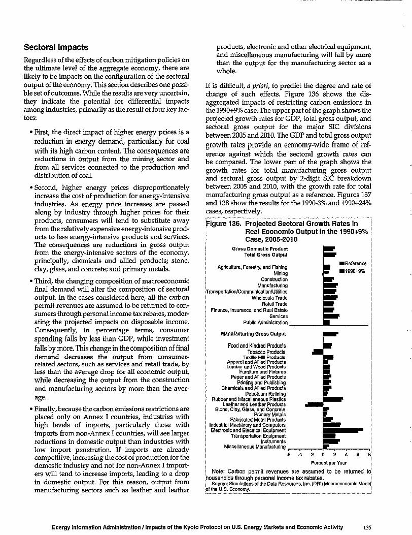
Sectoral ImpactsRegardless of the effects of carbon mitigation policies onthe ultimate level of the aggregate economy, there arelikely to be impacts on the configuration of the sectoraloutput of the economy. This section describes one possi-ble set of outcomes. While the results are very uncertain,they indicate the potential for differential impactsamong industries, primarily as the result of four key fac-tors:
• First, the direct impact of higher energy prices is areduction in energy demand, particularly for coalwith its high carbon content. The consequences arereductions in output from the mining sector andfrom all services connected to the production anddistribution of coal.
• Second, higher energy prices disproportionatelyincrease the cost of production for energy-intensiveindustries. As energy price increases are passedalong by industry through higher prices for theirproducts, consumers will tend to substitute awayfrom the relatively expensive energy-intensive prod-ucts to less energy-intensive products and services.The consequences are reductions in gross outputfrom the energy-intensive sectors of the economy,principally, chemicals and allied products; stone,clay, glass, and concrete; and primary metals.
• Third, the changing composition of macroeconomicfinal demand will alter the composition of sectoraloutput. In the cases considered here, all the carbonpermit revenues are assumed to be returned to con-sumers through personal income tax rebates, moder-ating the projected impacts on disposable income.Consequently, in percentage terms, consumerspending falls by less than GDP, while investmentfalls by more. This change in the composition of finaldemand decreases the output from consumer-related sectors, such as services and retail trade, byless than the average drop for all economic output,while decreasing the output from the constructionand manufacturing sectors by more than the aver-age.
• Finally, because the carbon emissions restrictions areplaced only on Annex I countries, industries withhigh levels of imports, particularly those withimports from non-Annex I countries, will see largerreductions in domestic output than industries withlow import penetration. If imports are alreadycompetitive, increasing the cost of production for thedomestic industry and not for non-Annex I import-ers will tend to increase imports, leading to a dropin domestic output. For this reason, output frommanufacturing sectors such as leather and leather
products, electronic and other electrical equipment,and miscellaneous manufacturing will fall by morethan the output for the manufacturing sector as awhole.
It is difficult, a priori, to predict the degree and rate ofchange of such effects. Figure 136 shows the dis-aggregated impacts of restricting carbon emissions inthe 1990+9% case. The upper part of the graph shows theprojected growth rates for GDP, total gross output, andsectoral gross output for the major SIC divisionsbetween 2005 and 2010. The GDP and total gross outputgrowth rates provide an economy-wide frame of ref-erence against which the sectoral growth rates canbe compared. The lower part of the graph shows thegrowth rates for total manufacturing gross outputand sectoral gross output by 2-digit SIC breakdownbetween 2005 and 2010, with the growth rate for totalmanufacturing gross output as a reference. Figures 137and 138 show the results for the 1990-3% and 1990+24%cases, respectively.
figure 136. Projected Sectoral Growth Rates ini Real Economic Output in the 1990+9%| Case, 2005-2010
•Reference
11990+9%
Gross Domestic ProductTotal Gross Output
Agriculture, Forestry, and FishingMining
ConstructionManufacturing
jTransportatlon/Communlcatlon/UfilitiesWholesale Trade
Retail TradeFinance, Insurance, and Real Estate
ServicesPublic Administration.
Manufacturing Gross Output
Food and Kindred ProductsTobacco Products
Textile Mill ProductsApparel and Allied ProductsLumber and Wood Products
Furniture and FixturesPaper and Allied Products
Printing and PublishingChemicals and Allied Products
Petroleum RefiningRubber and Miscellaneous Plastics
Leather and Leather ProductsStone, Clay, Glass, and Concrete
Primary MetalsFabricated Metal Products
Industrial Machinery and ComputersElectronic and Electrical Equipment
Transportation EquipmentInstruments
Miscellaneous Manufacturing-6 -4 -2
Percent per Year
Note: Carbon permit revenues are assumed to be returned tdhouseholds through personal income tax rebates.I Source: Simulations of the Data Resources, Inc. (DRl) Macroeconomic Modeof the U.S. Economy.
Energy Information Administration / Impacts of the Kyoto Protocol on U.S. Energy Markets and Economic Activity 135

Figure 137. Projected Sectoral Growth Rates inS Real Economic Output in the 1990-3%| Case, 2005-2010
•Reference
• 1980-3%
Figure 138. Projected Sectoral Growth Rates inReal Economic Output in the1990+24% Case, 2005-2010
Gross Domestic ProductTotal Gross Output
Agriculture, Forestry, and Fishing
MiningConstruction
j ManufacturingTransportation/Communication/Utilities
Wholesale TradeI Retail TradeI Finance, Insurance, and Real EstateI Services| Public Administration
i Manufacturing Gross Outputi| Food and Kindred Productsi Tobacco Products| Textile Mill Productsi Apparel and Allied Products| Lumber and Wood Productsi Furniture and Fixtures
Paper and Allied ProductsPrinting and Publishing
Chemicals and Allied ProductsPetroleum Refining
Rubber and Miscellaneous PlasticsLeather and Leather Products
Stone, Clay, Glass, and ConcretePrimary Metals
Fabricated Metal ProductsIndustrial Machinery and ComputersElectronic and Electrical Equipment
Transportation EquipmentInstruments
Miscellaneous Manufacturing
- 6 - 4 - 2
Percent per Year
Note: Carbon permit revenues are assumed to be returned tohouseholds through personal income tax rebates. j| Source: Simulations of the Data Resources, Inc. (DRI) Macroeconomic Modelbf the U.S. Economy. j
IReference
11990+24%
Gross Domestic ProductTotal Gross Output
Agriculture, Forestry, and Fishing
MiningConstruction
ManufacturingJTransportation/Communication/Utilities
Wholesale TradeRetail Trade
Finance, Insurance, and Real EstateServices
Public Administration
Manufacturing Gross Output
Food and Kindred ProductsTobacco Products
Textile Mill ProductsApparel and Allied ProductsLumber and Wood Products
Furniture and FixturesPaper and Allied Products
Printing and PublishingChemicals and Allied Products
Petroleum RefiningRubber and Miscellaneous Plastics
Leather and Leather ProductsStone, Clay, Glass, and Concrete
Primary MetalsFabricated Metal Products
Industrial Machinery and ComputersElectronic and Electrical Equipment
Transportation EquipmentInstruments
Miscellaneous Manufacturing
I Percent per Year
j Note: Carbon permit revenues are assumed to be returned tohouseholds through personal income tax rebates.| Source: Simulations of the Data Resources, Inc. (DRI) Macroeconomic Mode)bf the U.S. Economy.

7. Comparing Cost Estimates for the Kyoto Protocol
Introduction
This chapter provides a comparison of recent publiclyavailable estimates of the costs of achieving the KyotoProtocol carbon reduction targets in the United Statesfor the period 2008 to 2020. The projections are com-pared for the years 2010 and 2020, when the informationis available, for the following projection sources: theEnergy Information Administration (EIA) using theNational Energy Modeling System (NEMS), WEFA,85
Charles River Associates (CRA) using the Multi-Regional Trade model (MRT),86 the Pacific NorthwestNational Laboratory (PNNL) using the Second Genera-tion Model (SGM), the Massachusetts Institute of Tech-nology (MIT) using the Emissions Prediction and PolicyAnalysis Model (EPPA),88 Electric Power Research Insti-tute (EPRI) using the MERGE model89 and DataResources, Inc. (DRI).90 Differences between studies arerelated, to the extent possible, to the features of the mod-eling systems used (e.g., level of aggregation, level ofgeographic coverage), important assumptions em-ployed, and the particular points of view embodied inthe models.91
Two cases were solicited for analyses from each group: a7-percent-below-1990 (1990-7%) case in which theUnited States is assumed to reduce carbon emissions to1990-7% levels for the period 2008-2020 without thebenefit of sinks, offsets, international carbon permittrading, or the Clean Development Mechanism (CDM);and a best estimate of the impact on U.S. energy marketsif sinks, offsets, and Annex I emissions trading wereallowed, but not global trading or CDM.
Differences in the cost estimates for meeting the KyotoProtocol targets can be related to important differencesin assumptions about (1) economic growth in the refer-ence cases without the Kyoto Protocol, (2) the status ofthe resources available (e.g., resource base, world oilprices, and the slate of technologies available to the mar-ketplace), (3) the sensitivity of energy demand to pricechanges, (4) the degree of foresight that decisionmakershave in the marketplace, (5) the structure and function ofthe economy (e.g., how quickly the economy can shift toless energy-intensive industries when the price ofenergy relative to capital and materials increases), (6) thedegree and speed of substitution for factors of produc-tion (capital, labor, energy, and materials) when theirrelative prices change, and (7) the representation of tech-nology (i.e., representation of vintaged energy equip-ment and the penetration of new technologies).
Summary of ComparisonsBecause the information available varies considerably, adetailed comparison among the sources is virtuallyimpossible. Therefore, a comparison of commonvariables is provided in this section, with an explanationfor the differences between the sources. Comparisonsare provided for three of the cases analyzed in thisreport: the 1990-7% case and two cases—9 percentabove 1990 (1990+9%) and 14 percent above 1990(1990+14%)—that are comparable in some respects tothe Annex I trading case. The variables compared arecarbon price, change in actual gross domestic product(GDP) from the respective reference case in each study,
85 WEFA, Inc., Global Warming: The High Cost of the Kyoto Protocol, National and State Impacts (Eddystone, PA, 1998).^ Both the CRA and WEFA studies have been supported to some extent by industry groups, including the American Petroleum Insti-
tute.87 J.A. Edmonds et al., Modeling Future Greenhouse Gas Emissions: The Second Generation Model Description (Washington, DC: Pacific
Northwest National Laboratory, September 1992). Runs using PNNL's SGM model formed the basis for the testimony provided by Dr. JanetYellen, chairman of the Council of Economic Advisers, on March 4,1998, before the House Commerce Committee, Energy and Power Sub-committee.
88 H.D. Jacoby, R. Eckhaus, A.D. Ellerman, et al. "CO2 Emission Limits: Economic Adjustments and the Distribution of Burdens," EnergyJournal, Vol. 18, No. 3 (1997), pp. 31-58. MIT's analysis is part of a much larger integrated assessment methodology funded by the Office ofEnergy Research, U.S. Department of Energy.
89 A.S. Manne and R.G. Richels, "On Stabilizing CO2 Concentrations—Cost Effective Emissions Reduction Strategies," Energy and Envi-ronmental Assessment, Vol. 2 (1997), pp. 251-265. EPRI's work is self-funded and is part of the research agenda of electric utilities.
90 Standard and Poors DRI, The Impact of Meeting the Kyoto Protocol on Energy Markets and the Economy (July 1998).9* Information used in this chapter was contributed by Dr. Montgomery and Dr. Bernstein of Charles River Associates, Dr. Richels of the
Electric Power Research Institute, Dr. Edmonds of Pacific Northwest National Laboratory, and Professor Jacoby of MIT.
Energy Information Administration / Impacts of the Kyoto Protocol on U.S. Energy Markets and Economic Activity 137

actual and potential GDP loss, expenditures forpurchases of carbon emission permits, change in carbonintensity from the respective reference case, and changein fossil fuel consumption. Tables 30 and 31 providecomparisons of the results for 2010 and 2020. Furtherdetails are provided in Appendix C.
For the WEFA study, comparisons are provided onlywith the 1990-7% case. For DRI comparisons areprovided only for a trading case (Case 2). WEFA doesnot believe that sinks, offsets, or trading will be agreedupon and implemented before the target period of 2008to 2012, nor by 2020. As noted earlier in the report, EIAdoes not have the capability to analyze internationaltrading and thus is unable to provide a most likelyestimate of the impacts of the international tradingprovisions of the Kyoto Protocol, or of sinks and offsets,on the level of the energy-related carbon reductionsrequired to meet the 1990-7% reduction in greenhousegases. EIA's 1990+9% and 1990+14% cases are used inTable 31, because the carbon emissions levels of thosecases were most closely aligned with the other studiespresented.
Some of the major factors that result in differences in theprojected carbon prices and costs to achieve the 1990-7%carbon reduction level are:
• Relative differences in reference GDP and carbonemissions growth rates through 2020. For example,if the GDP or carbon emissions growth rate in agiven reference case is lower than that in EIA's refer-ence case, a smaller carbon reduction will be needed,and it will generally be easier to achieve the emis-sions target. If the reference GDP growth or carbonemissions growth is higher than in EIA's referencecase, the carbon price and GDP impacts relative tothose projected by EIA in this study will generally behigher. Most of the major differences among theanalyses are attributable to differences in the refer-ence case projections.
• Differences in assumptions about the potential foreconomical life extension or refurbishment ofexisting nuclear power plants beyond their normallicensing period. If, for example, no existing nuclearplants were retired by 2020, about 40 million metrictons of carbon emissions would be avoided from thecombustion of fossil fuel used in plants to replacethem.
• The amount of knowledge about future eventsassumed for decisionmakers. For example, modelsthat assume that decisionmakers have perfectknowledge about future prices, demands, or policiescould underestimate compliance costs, because allfuture events would be anticipated with certaintyand responded to at minimum cost. Analyses thatassume that all decisionmakers are myopic will tendto overstate transition costs.
• The amount of lead time decisionmakers areassumed to have to adjust to the Kyoto Protocol.For example, if a model starts to begin the adjust-ment process in 1985,1990 or 1995, it could underes-timate the costs of complying with the KyotoProtocol, because it has more time to adjust. Modelsthat wait until the last moment to begin the adjust-ments could overstate adjustment costs.
• The level of aggregation in the model for technolo-gies and goods. A model that deals only with aggre-gate products such as oil, gas, or coal without thebenefit of an explicit technology representation maynot capture important variables that can signifi-cantly affect energy efficiency and intensity or thechanging mix of industries that may result fromcompliance efforts.
• The amount of focus on the transition process andthe associated costs. For example, a model thatassumes that all capital and labor can be immediate-ly switched from one use to another cannot capturethe short-term or medium-term impacts of comply-ing with the Kyoto Protocol, because those costs arenot reflected in the model.
• The assumed speed and extent of changes that con-sumers can make in energy consumption ordemand for energy services in response to chang-ing prices (price elasticities of demand). Higherassumed elasticities make it easier to achieve the car-bon target through demand reductions. Lower elas-ticities make it more difficult.
Among the studies compared in Table 30, the projectedcarbon prices in 2010 fall into three groups. MIT, EPRI,CRA, and WEFA project prices in the range of $265(WEFA) to $295 (CRA) per metric ton of carbon. PNNLprojects carbon prices of about $221 per metric ton. EIAprojects carbon prices of $348 per metric ton.

In the PNNL study, assumptions about consumer priceresponsiveness (demand elasticities and capital/energysubstitution elasticities) are consistent with a long-termtime frame where everything is changeable.92'93 Apply-ing the long-term elasticities to the short-term andmid-term period can overstate the ease and willingness withwhich consumers change their equipment or reduce, . . . 94
their consumption in response to price increases.Further contributing to the low carbon price projection isthe amount of lead time consumers have to respond, aswell as differences in the reference case economicgrowth rates. The PNNL and EIA reference case GDPprojections are very similar. However, PNNL's end-userepresentation does not explicitly represent technolo-gies, and PNNL's assumed consumer responsiveness toprices (prompting lower energy service demand) andinterfuel substitution potential appear to be substan-tially higher in the medium term (through 2010) than theimplicit elasticities in EIA's explicit representation oftechnologies and consumer choices. The PNNL modelbegins solving in 1985 in 5-year increments. The PNNLreference case is calibrated to AEO98. In the PNNL pol-icy runs, the carbon policy was phased in over a 10-yearperiod beginning in 2000. Consequently, policy adjust-ments begin in 2001, consumers and producers begin toanticipate the Kyoto Protocol in that year, making theappropriate adjustments. In the PNNL analysis, electric-ity demand grows by 0.4 percent annually in the refer-ence case between 2010 and 2020. This is a significantdeparture from the annual growth rate of more than 2percent in recent years. Most electricity demand projec-tions have annual growth in excess of 0.9 percentbetween 2010 and 2020, as compared with PNNL's 0.4percent.95 Offsetting these factors are factors that tend tooverstate cost. For example, in the PNNL analysis, pri-mary renewable use for generation changes only slightlyfrom the reference case in 2020, even with a carbon priceof $286 per metric ton.
The group of models projecting costs between $265 permetric ton and $295 per metric ton in 2010 for the 1990-7% case include transitional processes and costs—eitherin the macroeconomy or in the energy system—througha detailed representation of the cost, performance, andmarket adoption of technologies.96 This group includesthe CRA model. Through 2010, CRA projects that, in thereference case, U.S. GDP will grow by $270 billion morethan projected in most of the other studies compared.The higher growth rate of GDP normally makes thereduction in emissions harder and more costly to theU.S. economy.
If differences in the reference cases were the only factoraccounting for the different estimates of the costs ofcomplying with the Kyoto Protocol, then CRA's costswould exceed EIA's and WEFA's in 2010; however, largeeconometric models of the U.S. economy like those ofWEFA and DRI tend to focus on the transitional process,including the method of recycling any carbon fees thatmay be collected by the Federal Government, and unem-ployment that may be increased as a result of policyimplementation. The WEFA, EIA, and DRI analysesassume that labor can be dislocated, whereas most otheranalyses assume full employment97 despite the suddenreduction of energy resources. More aggregated worldanalyses, including the CRA, PNNL, EPRI, and MITstudies, omit such details, because the inclusion ofglobal regional coverage and trade flows requires sim-plifications (some important) in the detail with whicheach region is represented. Model aggregation tends tounderestimate the macroeconomic costs; on the otherhand, a lack of global coverage (as in the EIA, DRI, andWEFA models) may overstate transition costs, particu-larly if international trading is implemented efficiently.Also, fossil fuel consumption in 2010 in the CRA analy-sis is about 6 quadrillion British thermal units (Btu) lessthan in the EIA reference case, with virtually identicalcarbon emissions levels, suggesting an accounting dif-ference in emissions coefficients.
9 2 The PNNL study uses a dynamic-recursive, computable general equilibrium (CGE) model with neoclassical elements. A model is a"general equilibrium" model if it represents all parts of the economy, both energy and non-energy, and all markets clear (supply equals de-mand at the prices determined). The model is "computable" if a computer is used to solve for the equilibrium; it is "dynamic" if it keepstrack of variables over time. A model is "neoclassical" if the model structure assumes that (1) its economic agents have perfect foresight andknowledge of all past, present, and future events, (2) there is perfect and instantaneous ability of capital and labor to move between uses andsectors, and (3) such transitions are costless and instantaneous.
9 3 The PNNL model (SGM) can be run with either perfect or imperfect foresight. Labor and new capital move freely.9 4 A carbon price of $221 per metric ton in 2010 would increase the delivered electricity price by 49 to 69 percent and reduce electricity
consumption by 22 percent relative to PNNL's reference case. This implies that, on average, consumers will reduce consumption of electric-ity by 3.2 to 4.5 percent for every 10-percent increase in the price of electricity. In 2020, a carbon price of $286 per metric ton translates to anelectricity price increase of 59 to 66 percent, resulting in a 28-percent reduction in electricity consumption. This implies that consumptionwill decline by about 4.2 to 4.7 percent for every 10-percent increase in price. (The estimated electricity price changes were derived fromcomparable EIA cases.)
9"* For example, WEFA's annual electricity growth rate is 1.7 percent and EIA's is 0.9 percent.9(^ The WEFA, CRA, MIT, and DRI models are econometric, general equilibrium, macroeconomic models. WEFA and DRI model the
United States, CRA and MTT model the world.9 7 The full employment assumption means that the unemployment rate is unchanged from reference case levels.
Energy Information Administration / Impacts of the Kyoto Protocol on U.S. Energy Markets and Economic Activity 139

Table 30. Comparison of Results for Reducing Carbon Emissions to 7 Percent BelowWithout Trading, Sinks, Offsets, or Clean Development Mechanism
Projection
Carbon Price (1996 Dollars per Metric Ton) . . .
Change in Actual Gross Domestic ProductFrom Reference Projection
Percent
Billion 1996 Dollars
Loss in Potential Gross Domestic ProductRelative to Reference Projection(Billion 1996 Dollars)
Change in Carbon Intensity (Percent)Change in Fossil Fuel Consumption (Percent)...
MIT
266
-1.5b
-156
NA
NA
NA
I EPRla |
2010
280
-1.0-102
73
-27.9-19.3to-23.9d
2020
CRA
295
-2.1
-227
82-32
-30.3
ElA
348
-4.2
-437
79 to 94°-26
-22.1
1990 Levels
PNNL |
221
NANA
65
-31
-24.5
WEFA
265
-3.2
-332
60
-24.5
-20.9
| Carbon Price (1996 Dollars per Metric Ton) . . .
I Change in Actual Gross Domestic Producti From Reference Projection
| Percent| Billion 1996 DollarsI Loss in Potential Gross Domestic ProductI Relative to Reference Projection
(Billion 1996 Dollars)
I Change in Carbon Intensity (Percent)
I Change in Fossil Fuel Consumption (Percent)...
147
-1.5D
-156
NA
NA
NA
251
-0.96-120
81
-32.2
-24.0 to -32.3e
316
-2.4-311
111
-31.0
-35.1
305
-0.8-91
75 to 103°
-38.9
-25.7
286
NANA
109-36.9-29.6
360
-2.0-257
130
-35.9
-28.4
fEPRI allows 50 million metric tons for sinks in this case.^"he percentage represents MITs upper bound estimate, including some macroeconomic adjustment costs. MIT provided a range from -0.5 to
-1.5 percent for change in GDP, to be interpreted as minimum and maximum losses to the economy. For the purposes of this chapter, the lowesirange is the irreducible economic loss. Because GDP was not provided forthe MIT reference case, the reader may assume a central value for GDP oi$9,400 billion in 2010 and $10,900 in 2020 (1992 dollars). Consequently, the range of losses is $52 billion to $156 billion in 2010 (1996 dollars).j °The losses in potential GDP for ElA shown in Tables 30 and 31 use two different concepts, which give slightly different results. One uses the com-putation of potential GDP that is derived from the DRI model as described in Chapter 6 of this report. The second uses the approximation methodunder the carbon reduction versus carbon price curve, also discussed in Chapter 6. The two calculations produce nearly identical results for the 1990-!J3% case. For the 1990-7% case, the DRI calculation produces a smaller estimate of potential GDP losses. For all other cases, the DRI calculation!produces a higher estimate of potential GDP losses. Because the projections from analyses other than ElA's were calculated using the approximation;method related to the carbon reduction versus carbon price curve, estimates from both the DRI and approximation methods are provided forthe ElAstudy.| Only total primary energy was provided. Fossil fuel consumption was derived by subtracting an estimate for nuclear energy and renewable energyRanging from 13 to 17 quadrillion Btu from total primary energy for 2010.! eOnly total primary energy was provided. Fossil fuel consumption was derived by subtracting an estimate for nuclear energy and renewable energ;of 12 to 20 quadrillion Btu from total primary energy for 2020. j| NA = not available. j| Sources: ElA: National Energy Modeling System, run FD07BLW.D080398B. WEFA: WEFA, Inc., Global Warming: The High Cost of the Kyoto Protocol, National andState Impacts (Eddystone, PA, 1998). PNNL: E-mail of data from PNNL with explanation of GDP effect received from Ronald Sands of PNNL on August 26,1998. CRA:Paul M. Bernstein, Charles River Associates, e-mail communications, August 24,1998. EPRI: E-mail provided by R. Richels of EPRI on July 6,1998. MIT: Facsimile datedJuly 10,1998, from Prof. Henry Jacoby, MIT, Cambridge Massachusetts. j

Table 31. Comparison of Results for Reducing Carbon Emissions to 7 Percent Below 1990 LevelsWith Annex I Trading, Sinks, and Offsets
Projection MIT EPRIa
2010
CRA DRI Case 2
EIAb
1990+9% | 1990+14% PNNL
> Carbon Price (1996 Dollars per Metric Ton) . . .; Change in Actual Gross Domestic Product| From Reference Projection
i Percenti Billion 1996 Dollars
: Loss in Potential Gross Domestic Product! Relative to Reference Projection! (Billion 1996 Dollars)
j Irreducible Losses (Billion 1996 Dollars)
! Expenditures on Annex I Trading! (Billion 1996 Dollars)I Purchased Emissions Creditsj (Million MetricTons)0
j Change in Carbon Intensity (Percent)
; Change in Fossil Fuel Consumption (Percent)...
175
-1.5
NA
NA
NA
NA
NA
NA
NA
114
-0.5
-56
17
43
-26
229
-15.7
-13.2
109
-1.3
-133
1546
-31
288
-15.8
-14.6
110
-1.1
-118
1632
-16
147
-15.8
-11.7
163
-2.0
-207
27 to 3653 to 62
-26
161
-15.8
-12.7
129
-1.7
-177
17 to 29
47 to 59
-30
229
-12.9
-10.3
100
NANA
38
55
-17
171
NA
-16.8
2020
j Carbon Price (1996 Dollars per Metric Ton) . . .
| Change in Actual Gross Domestic ProductI From Reference Projectioni Percent| Billion 1996 Dollars| Loss in Potential Gross Domestic Product! Relative to Reference Projection| (Billion 1996 Dollars)
! Irreducible Losses (Billion 1996 Dollars)
! Expenditures on Annex I Trading| (Billion 1996 Dollars)I Purchased Emissions Creditsi (Million MetricTons)0
i Change in Carbon Intensity (Percent)
j Change in Fossil Fuel Consumption (Percent)...
119 188 175 131 141 123 142
-1.5NA
NANA
NA
NANANA
-0.96-120
44
73
-33
177
-22.8
-18.7
-1.7-226
42
82
-40
228
-18.8
-23.3
-0.3-41
31
46
-15
111
-23.5
-19.3
-0.6-76
33 to 43
56 to 66
-23
161
-22.2
-16.2
-0.5-63
24 to 35
52 to 63
-28
229
-20.1
-14.2
NA
NA
71
102
-31
219
NA-20.6
fEPRI allows some contribution from the CDM.I nThe 1990+9% and 1990+14% cases are shown for comparison only, because the carbon emissions levels projected in these cases are nearthose of the other studies shown.| cFor EIA and EPRI, purchased carbon emissions credits equal the difference between the emissions target and 1,306 million metric tons (3 percentpelow the 1990 carbon emissions level).j NA = not available.| Sources: EIA: National Energy Modeling System, runs FD09ABV.D080398B and FD14ABV.D080398B. CRA: Paul M. Bernstein, Charies River Associates, e-mailcommunications, August 24,1998. EPRI: E-mail provided by R. Richels of EPRI on July 6,1998. DRI: Standard and Poors DRI, The Impact of Meeting the Kyoto Protocolpn Energy Markets and the Economy (July 1998). MIT: Facsimile dated July 10,1998, from Prof. Henry Jacoby, MIT, Cambridge Massachusetts. PNNL: Ronald Sands,pNNL, e-mail communication, August 26,1998.
Energy Information Administration / Impacts of the Kyoto Protocol on U.S. Energy Markets and Economic Activity 141

Because of the aggregation of sectors and outputs in theCRA analysis, CRA's analytical approach is likely tounderestimate the costs of the Kyoto Protocol. In theCRA reference case GDP grows rapidly from 2010 to2020, making it more difficult to comply with the KyotoProtocol in the 1990-7% case. Hence, the carbon price isprojected to rise to $316 per metric ton in 2020.
WEFA projects reference case GDP that is about 1.3 per-cent lower than EIA's in 2010 but then rises above EIA'sby about $670 billion, or about 6 percent, by 2020. Thedifference in the carbon prices in 2010 between the twostudies ($265 per metric ton for WEFA and $348 per met-ric ton for EIA) is largely attributable to (1) a lower refer-ence case GDP and lower emissions in the WEFA study,so that smaller reductions are needed to comply with the1990-7% target, and (2) differences in the mix of fuelsused in the reference case to generate electricity. WEFA'sanalysis projects less coal and more gas use for electric-ity generation than EIA's analysis, with basically thesame electricity demands in 2010.
In 2020, the WEFA carbon price rises to about $360 permetric ton—about $55 per metric ton higher than theEIA carbon price for the same case. The reason for thisdifference is based on three factors. Differences in thereference case GDP growth rates (WEFA's GDP growsmuch faster than EIA's from 2010 to 2020) lead to theneed for higher fuel prices in the WEFA projection tocomply with the 1990-7% case. WEFA assumes thatnuclear life extensions would not be economical orfeasible, whereas EIA allows economical nuclear re-furbishments. WEFA projects that renewables cannotcontribute significantly to electricity generation: re-newable use for generation increases by only 11 percentin 2020 relative to the baseline, even with a carbonprice of $360 per metric ton, whereas EIA projects a 115-percent increase in the use of renewables for elec-tricity generation in the 1990-7% case relative to the EIAreference case.
The EPRI analysis begins to react to the Kyoto Protocolin 1990, resulting in lower carbon prices and GDP lossesthan in the EIA analysis for 2010." Further, since themodel does not have end-use technology detail, the rateof autonomous energy efficiency improvement isassumed as a policy lever and is based on the analyst'sjudgement or on calibration with other midterm,technology-rich models.
The pattern of carbon prices in the MIT study is similarto that in the EIA and EPRI studies. In the MIT analysis,decisionmakers do not see future prices or the impend-ing Kyoto Protocol. In addition, capital stock is vin-taged—i.e., once capital is invested in equipment, thatcapital is sunk and the technology's efficiency and usecannot change during its survival period.
Carbon prices in 2020 for the 1990-7% case are moreevenly distributed among the studies, ranging between$147 per metric ton for MET to about $360 per metric tonfor WEFA. The declining carbon prices in the EPRI andEIA studies result from the projected increasing penetra-tion of carbon-free or low-carbon generation technolo-gies, coupled with greater selection of more efficienttechnologies that become economical with higher end-use fuel prices. MIT's carbon price in 2020, $147 per met-ric ton, is the lowest because this study implicitly hasgreater optimism than EIA and EPRI that the economywill produce and adopt low-carbon or carbon-free tech-nologies by 2020.
As already mentioned, the lead time that decisionmak-ers have to anticipate the Kyoto Protocol and theassumed responsiveness of consumers and equipment(demand elasticities and fuel substitution elasticities)can significantly affect the projections of how costly anddifficult the transition will be. Most of the studies com-pared, with the exception of WEFA and EIA, allow thetransitions to begin as early as 1990 or 1995.100 Sincestarting earlier allows consumers and producers to reactearlier, the economy has more time to adjust to theKyoto Protocol. This may result in an underestimationof the carbon prices and the midterm actual GDP lossesto the economy that will be required to achieve the 1990-7% case.
The CRA, WEFA, and PNNL studies exhibit a risingtrend in the carbon prices required over time to maintainthe 1990-7% emissions target, because technologicalimprovements do not occur quickly enough relative todemand growth. The technology-rich studies reach theirpeak carbon price in the early part of the complianceperiod, followed by a flat or declining carbon price to2020 as more efficient technologies are adopted. Therelatively high energy prices make higher-efficiency andhigher-cost equipment more competitive in the early
part of the compliance period and give rise to normallearning through manufacturing experience, which
9 8 The CRA model uses perfect foresight for investment behavior, which may also contribute to underestimating the costs. It assumesthat products (like gas and coal) are not perfect substitutes and capital is not perfectly malleable. Further, the demand for energy is onlymoderately responsive to price changes, compared to the PNNL model. CRA develops its model parameters using the GTAP database fromPurdue University and the International Energy Agency (DBA) database.
9 9 EPRI's MERGE model is an Aggregate Optimization Model and has perfect foresight. The EPRI model is being rebenchmarked tostart in 2000 and should result in higher carbon prices and higher GDP losses in 2010 than are shown in their current analysis.
100For PNNL, since the model begins solving in 1985, policy instruments could be introduced as early as 1990. For this study, PNNL re-ports that the policy instruments for the Kyoto Protocol were phased in beginning in 2001.
helps to reduce equipment costs in the later part of thecompliance period.
The other major area of disagreement among the projec-tions is the impact on actual GDP. In 2010, actual GDPlosses relative to each reference case range from -1.0 per-cent (EPRI) at the low end to about 4.2 percent (EIA) atthe high end. Some economists have noted that the totalGDP impact on the U.S. economy of regulatory pro-grams such as the Kyoto Protocol are large, and that thetrue costs typically exceed direct costs by a factor of twoto four, particularly in the few years following imple-mentation.101 CRA projects a 2.1-percent loss in GDP in2010 and a 2.4-percent loss in GDP in 2020. This contrastswith the EIA projection of a 4.2-percent loss in GDP in2010 and a 0.8-percent loss in 2020, a trend returning tothe reference case GDP. The EIA projected recoverytrend is due to declining real prices after 2012, whereasincreasing GDP losses for CRA are due to continuedincreasing delivered energy prices throughout the pro-jection period and the relative high GDP level in the ref-erence case from which the reductions must be made.
Most of the reasons for the differences in carbon pricesalso contribute to the differences in GDP losses. Forexample, perfect foresight and long lead times allow theeconomy to adjust at minimum cost as in the PNNL,EPRI, and CRA models. In the WEFA analysis, lowerGDP growth in the early period allows for lower carbonprices and smaller GDP losses relative to the EIA study.CRA's lower carbon price and smaller GDP losses areattributable to four factors: (1) the lack of representationof a revenue recycling mechanism, (2) the high level ofaggregation of the U.S. energy-economy, (3) the lengthof the adjustment period, and (4) the incorporation ofinternational trade flows.
The GDP losses portrayed in the analyses are not basedon the same definitions. EIA, DRI, and WEFA reportlosses in potential GDP102 and full macroeconomic ad-justment costs. CRA and EPRI report losses to potential
GDP plus some but not all of the macroeconomic adjust-ment costs, because the level of aggregation used to rep-resent the U.S. macroeconomy does not permit a fullrepresentation of the macroeconomic adjustment costs.PNNL reports only the direct cost of meeting therequired commitment level, i.e., losses in potential GDP.The loss in potential GDP can be estimated for all thestudies except MTT and can be combined with paymentsfor international permits to develop "irreducible" lossesto the economy arising from compliance with the KyotoProtocol for each of the two cases (no trading and AnnexI trading).103 Estimates of irreducible losses to GDP inthe 1990-7% case in 2010 are remarkably close, rangingfrom $60 billion for WEFA to about $94 billion for EIA(in 1996 dollars). The range of irreducible losses in 2020is $75 billion for EIA to $130 billion for WEFA. WEFAprojects the largest potential loss in 2020 because it hasthe highest carbon prices and its reference case projec-tion of GDP in 2020 is one of the two highest.
The GDP comparisons imply that there is a great deal ofuncertainty about the actual economic losses that couldresult from adherence to the Kyoto Protocol, with actualeconomic losses rising to as high as 4.2 percent of refer-ence case GDP in 2010—particularly for analyses thatuse highly disaggregated representations of the U.S.economy (EIA and WEFA). The difference betweenactual losses and potential GDP losses represents macro-economic adjustment costs, which are viewed by econo-mists as theoretically reducible by optimal fiscal andmonetary policies. This maybe another factor leading tothe wide variation in estimates of macroeconomicadjustment costs. Nevertheless, there is considerableagreement on the level of the potential GDP losses.
All the studies are in close agreement on the change incarbon intensity that must occur relative to each refer-ence case. Reductions in carbon intensities are between24 percent and 29 percent in 2010 and between 32 per-cent and 39 percent in 2020.
101 Jorgenson and Wilcoxen, "Impact of Environmental Legislation on U.S. Economic Growth and Capital Costs," in U.S. EnvironmentalPolicy and Economic Growth: How Do We Fare? (Washington, DC: American Council on Capital Formation, 1992); "Reducing U.S. CarbonEmissions: An Econometric General Equilibrium Assessment," Resource and Energy Economics, Vol. 15 (1993), pp. 7-25; and P.M. Bernsteinand W.D. Montgomery, "How Much Could Kyoto Really Cost? A Reconstruction and Reconciliation of Administration Estimates" (CharlesRiver Associates, 1998).
102"j ,e CUjve shown in Figure 114 in Chapter 6 of this report summarizes the relationship between the level of control and the marginalcost of that level of control. Hence, at each increment of control, the marginal cost is by definition equal to the economic resources that mustbe forgone in order to achieve the increment in control. It follows, therefore, that the sum of the marginal costs must equal the total cost of thecontrols that would be internalized in markets. This is the integral of the area under the curve, shown as area A in Figure 114. Conceptually,this is essentially the same effect that is measured by the unavoidable cost in the reduction of potential GDP in the macroeconomic models.As shown in Figure 115, this measure of the unavoidable costs using the results of the NEMS model is nearly identical to the similar estimatefrom the DRI macroeconomic model.
•^Furthermore, for the balance of total emissions needed to meet the Kyoto targets, permits would be purchased on the internationalmarket. If the marginal cost of control in the United States and the international prices of permits are in equilibrium, then the area B in Figure114 will represent the total payments for permits, and the sum of the two parts will represent the irreducible losses to the economy underthat trading regime to meet the Kyoto requirements.
Energy Information Administration / Impacts of the Kyoto Protocol on U.S. Energy Markets and Economic Activity 143
Comparisons of Annex I Trading Cases
Only five analyses—MIT, EPRI, CRA, PNNL, andDRI—provided simulations of the impacts of sinks, off-sets and Annex I trading. DRI's Case 2 is compared withthe other Annex I trading cases because carbon permitspurchased abroad are closest, falling in the range of 147to 288 million metric tons.104 Two EIA cases—1990+9%and 1990+14%—are compared with those studies inTable 31, because both of these cases yield carbon emis-sions in the range of the other studies. Internationallypurchased carbon credits in 2020 fall in the range of 111to 229 million metric tons for all these analyses. EIA'scarbon prices in the 1990+9% case is $163 per metricton105 in 2010 and $141 per metric ton in 2020. The EIAcarbon price in the 1990+14% case is $129 per metric tonin 2010 and $123 per metric ton in 2020. MTT providedonly carbon prices and a range of GDP losses; thus, fur-ther comparisons are not possible.
EIA's purchased carbon credits in 2010 (229 million met-ric tons) in the 1990+14% case are closest to the projectedinternational purchased credits by EPRI and CRA (229and 288 million metric tons, respectively). The carbonprice projected in these cases ranges from $109 per met-ric ton for CRA to $129 per metric ton for EIA, a statisti-cally insignificant variation. While there is considerableagreement on the carbon price and credit purchases inthese analyses, actual GDP losses projected in EIA's1990+14% case are more than 200 percent higher thanthe actual GDP losses projected by EPRI and more than33 percent higher than CRA's. It is also about 50 percenthigher than DRI's.
In the Annex I trading cases, only the DRI and EIAanalyses consider how the domestic funds will be recy-cled back to the economy. EIA assumed that the reve-nues from domestic sales of carbon emission permitswould be recycled back to consumers through a per-sonal income tax rebate, as described in Chapter 6,106
and DRI assumes a return of funds to business. The DRIchoice of returning the carbon revenues to business pro-vides a significant boost to business investment in theeconomy, which implies higher business profits andlower real incomes for consumers in the medium term.According to the DRI analysis, returning carbon reve-nues to business ultimately would accelerate recovery
and lead to stronger economic growth in the longer termthan would recycling the carbon revenues to consumers.The impacts of the two recycling mechanisms accountfor most of the differences in macroeconomic resultsbetween the EIA and DRI analyses.
The DRI approach also phases in the carbon policy overa 10-year period (an approach necessitated by the struc-ture of the DRI energy model), whereas EIA phases inthe policy over a 3-year period. This factor adds to thedifference between the EIA and DRI analyses of mac-roeconomic costs. In the DRI study, the 10-year phase-inand the assumption that consumers will anticipate andrespond to the Kyoto Protocol early results in asmoother economic transition and tends to give a lowercarbon price than analyses with shorter phase-in periodslike EIA's.
The estimates of unavoidable (irreducible) losses—income losses that cannot be recovered—for the U.S.economy range from $32 billion (DRI Case 2) to about$62 billion (EIA) in 2010. There are many frictions thatcan increase costs above the irreducible minimum.These include business cycles, international trade andcapital constraints, regulation, use of imperfect instru-ments instead of auction permits, coal subsidies, CAFEstandards, exemptions, efficiency losses from taxation,etc.107 Various Federal Reserve and Federal Governmentpolicies might mitigate actual GDP losses. There is con-siderable uncertainty regarding all the above actions.
The EPRI analysis, because of its perfect foresight andoptimizing framework, yields actual GDP losses that areclosest to its estimated unavoidable losses. CRA esti-mates actual GDP losses that are almost 3 times itsunavoidable losses in 2010, and estimated actual GDPlosses in 2010 for the DRI and EIA 1990+14% cases are 3to 4 times the unavoidable losses. Because DRI's andEIA's actual GDP losses are based on a detailed mac-roeconomic model that has limited foresight, focuses onthe transitional process rather than the steady-state con-dition of the economy, their projected GDP losses areexpected to be the largest and perhaps more appropriatein the mid term (through 2010). WEFA and EIA incorpo-rate revenue recycling, while DRI redirects the revenuesthrough higher profits to business.
104Standard and Poors DRI recently analyzed three cases for the UMWA-BCOA LMPCP Fund. Case 1 assumed that 8 percent of the nec-essary carbon reduction in 2010 would be accomplished from sinks and offsets, 15 percent from trading, and 77 percent domestically. Case 2assumed that sinks and offsets would account for 12 percent of the required reduction from baseline in 2010,30 percent would be purchasedfrom abroad, and 58 percent would be accomplished domestically. Case 3 assumes that sinks and offsets would generate 16 percent of the re-quired reductions from baseline, 55 percent of the reduction would be purchased from abroad, and 29 percent of the reduction to be accom-plished within domestic energy markets. Given that the DRI baseline for 1990 carbon emissions is 1,336 million metric tons, the domestictarget for Case 1 in 2010 (1,354 million metric tons) is about 1 percent above 1990 levels, Case 2 (1,452 million metric tons) is about 9 percentabove 1990 levels, and Case 3 (1,593 million metric tons) is about 19 percent above 1990 levels.
105For simplicity and ease of exposition, it is assumed in this chapter that the carbon price, the price at the margin that the United States iswilling to pay to reduce carbon emissions, equals the internationally traded permit price.
106In Chapter 6, EIA also considers a social security tax rebate.107Tom Tietenberg, Environmental and Natural Resource Economics, Third Edition (Harper Collins Publishers, 1992).
of the U roto Protocol on U.S. Enen Markets and Economic Activil

The DRI and EIA analyses share the same DRI mac-roeconomic model; however, they differ in the way theyrepresent the energy market. DRI uses a largelyeconometric approach, with some technology compo-nents to simulate equipment turnover. Responses ofenergy demand to energy prices are approximatedthrough demand elasticities. Elasticity estimates canvary dramatically and are a major factor in determiningresults.
Because DRI and EIA share the same macroeconomicmodel, the reference case estimates of macroeconomicvariables are nearly identical for 2010. The differences inthe reference case energy projections are primarily dueto differences in fuel prices. By 2020, the differencesbetween the DRI and EIA macroeconomic projectionswiden as differences in fuel prices widen.
The EIA 1990+9% case reduces more emissions domesti-cally (325 million metric tons) than the 1990+14% case atan average carbon price of $159 per metric ton (peakingat $163 per metric ton) for the 2008-2012 period. Theunavoidable losses to the U.S. economy for 2010 are esti-mated to be slightly ($3 to $6 billion) more than in the1990+14% case. The actual GDP losses are more than 3.5times the unavoidable losses in the EIA cases.
The carbon price in the two EIA cases and the MTT trad-ing case declines from 2010 to 2020, unlike the carbonprices in the EPRI, CRA, and DRI analyses that increaseover the decade. Most of the reasons for these differ-ences have already been described in the 1990-7% com-parison case and will not be repeated here. However,one noteworthy difference remains—the availabilityand cost of Annex I carbon permits and internationaltrade. In the EPRI model, inexpensive permits are pre-sumed to be available from Russia in the early part of theKyoto Protocol implementation period but are assumednot to be available in the later part of the period. Theelimination of the easy Russian permits makes it harder
for the United States to meet its commitments in 2020through Annex I trading and raises the carbon permitprice by 65 percent relative to 2010. The reason for the60-percent increase in 2020 in the CRA carbon price isrelated to the differences in the representation ofadvanced technologies, the level of aggregation of theCRA model as previously discussed, and the absence ofeasy carbon permits from Russia.
The Administration's estimate of the costs of implement-ing the Kyoto Protocol109 has been developed, in part, byusing the PNNL model. The Administration's analysisdoes not provide sufficient data to be included in Tables30 and 31; however, the Administration asserts in Table4 of the analysis (page 52) that under Annex I trading,
the carbon price wouldbe reduced by 11 percent and theresource cost •would be decreased by 57 percent relativeto a case in which all carbon reductions are achieveddomestically. Using Tables 4 and 5 on pages 52 and 53 ofthe Administration's report on the Kyoto Protocol, thecarbon price for the 1990-7% case can be calculated to be$192 per metric ton (in 1996 dollars), and the irreducibleeconomic losses can calculated to be $60 billion. WhenAnnex I trading is assumed, the Administration projectsthat carbon prices would be reduced to $54 per metricton, with $26 billion dollars of irreducible losses.110 Therelatively lower GDP growth rate from 1995 to 2010 inthe Administration's reference case analysis—2.1 per-cent annually, compared with 2.3 percent in the AEO98reference case, is a major factor that results in a lowercarbon price and lower economic costs needed toachieve a carbon target.
Based on Tables 30 and 31, the following can be summa-rized:
• There is no clear consensus on how effective Annex Itrading will be in reducing carbon prices andthe costs to the United States. WEFA believes thatAnnex I trading will not be effective at all because of
1(^Other reference case differences that influence the Kyoto analysis include: (1) The DRI reference case projects 3.1 quadrillion Btulower primary energy consumption and 1.8 quadrillion Btu lower fossil fuel consumption in 2010 than does EIA. By 2020, the differencesgrow to 4.2 quadrillion Btu of primary energy and 2.4 quadrillion Btu of fossil fuel consumption. Associated carbon emissions are alsolower. Consequently, it should be less costly for the economy to achieve the same carbon target (1,452 million metric tons) in the DRI analy-sis than in the EIA analysis (1,461 million metric tons in 1990+9% case), as Table 31 confirms. (2) The DRI reference case projects higher worldoil prices, higher delivered coal prices, and lower gas prices than the EIA reference case and greater coal, lower gas, and lower oil consump-tion than the EIA reference case for 2010 and 2020. The differences in the mix of fuel consumption are related to the differences in fuel pricesin the cases. Because the delivered price that consumers react to is the sum of the fuel costs plus the carbon price, when oil and coal prices arehigher (without the carbon price), the additional carbon price required to achieve the same delivered coal and petroleum product prices willbe lower. Higher reference case prices imply lower required carbon prices to induce an energy demand or mix change. Lower carbon pricesusually result in lower economic losses.
1 0 9 The Kyoto Protocol and the President's Policies To Address Climate Change: Administration Economic Analysis (Washington, DC, July 1998).HO According to Table 5, page 53, of the Administration's report, Annex I trading with participation by key developing countries would
result in a permit price of $23 per metric ton and irreducible losses of $12 billion. Table 4 on page 52 of the report indicates that the permitprice in that case would be reduced by 88 percent and the resource cost would be reduced by 80 percent relative to a "domestic onh/" case.This means that 12 percent of the carbon price for the domestic only case would be $23, and thus the carbon price in the domestic only casewould equal $192 per metric ton. Similarly, 20 percent of the domestic only resource cost would be $12 billion, meaning that the domesticonly resource cost would be $60 billion. Using the percentages for Annex I trading in Table 4, the carbon price and the irreducible losses canalso be derived for the Annex I trading case.
Energy Information Administration / Impacts of the Kyoto Protocol on U.S. Energy Markets and Economic Activity 145

political and implementation difficulties. Others,like CRA, EPRL and PNNL, suggest that carbonprices in 2010 can be reduced by about 60 percent.
1 All the studies project irreducible losses to the econ-omy that are small (less than 1 percent of GDP in2010 and 2020) in absolute magnitude—between $32billion and $62 billion in 2010 and between $46 bil-lion and $102 billion in 2020. The wider differencesin 2020 reflect the different perspectives on produc-tion losses to the economy associated with forcedreductions in fossil fuel energy use.
1 With Annex I trading, estimated actual GDP lossesrelative to each reference case range from 0.5 percentto about 2 percent.
1 If the United States is required to achieve stabiliza-tion at the 1990-7% levels, the estimate of carbonprices required for stabilization in 2010 range from alow of $221 per metric ton to $348 per metric ton,with the vast majority in the $265 to $295 per metricton range. Actual GDP losses are projected to rangefrom 1.0 percent to 4.2 percent. However, since allthe studies except EIA's and DRI's assume early U.S.action (before 1998) to limit carbon emissions, theirestimates of carbon prices and GDP estimates arelikely to be low.
The "Five-Lab Study"
Five U.S. Department of Energy Laboratories wereasked in the winter of 1996-97 (before the Kyoto confer-ence) to develop technology-oriented strategies forreducing U.S. carbon emissions to 1990 levels by 2010.111
To represent the potential impact of new technologystrategies on carbon emissions, the study assumesincreased performance and lower costs for new tech-nologies, new government policies that promote theiradoption into the market, and a greater propensity byconsumers to buy them than they have shown in thepast. In addition, the Five-Lab Study assumes the lowereconomic growth (and lower carbon emissions) in theAnnual Energy Outlook 1997 than the EIA analysisdescribed in this report.
The principal components of the Five-Lab Study focuson the adoption of energy-efficient technologies underthe assumption of a $25 and $50 per metric ton domesticcarbon price; an aggressive research and development(R&D) program; and aggressive but unspecified newpolicies to facilitate adoption of energy-efficient tech-nologies. The analysis was produced using a series ofindependent end-use sector models that were manuallycoupled to an electricity market model that assumes aderegulated electricity market.112 Thus, feedbackbetween energy markets and the rest of the economywere not captured. Consequently, the individual sectorsolutions may be inconsistent with each other and mostlikely do not represent a market equilibrium.
The Five-Lab Study is not directly comparable with anyof the analyses compared above, because it was not pre-pared using an integrated modeling framework thatsimultaneously balances the energy demand for equip-ment and consumption made by consumers in all seg-ments of the economy with the supply and prices offuels and economic growth. Therefore, simple compari-sons between the Five-Lab Study and EIA's analysis canbe misleading.
Given all the above qualifications, three comparisons aremade between the Five-Lab Study and the EIA analysis(Tables 32 and 33). The Five-Lab Study is compared interms of (1) the EIA case that comes closest to achieving acarbon price of $50 per metric ton in 2010 (the 1990+24%case), (2) the EIA case that comes closest to reducingcarbon emissions by about the same amount relative toits baseline (the 1990+9% case), and (3) the EIA case thatfocuses on advanced technologies (the 1990+9% hightechnology sensitivity case). By design, none of the Five-Lab Study scenarios results in carbon emissions that arebelow 1990 levels, because they were targeted toachieving stabilization at 1990 levels.
The Five-Lab Study defines three scenarios: (1) an effi-ciency case, (2) a high efficiency/low carbon case with a$25 per metric ton carbon price (25 HE/LC), and (3) ahigh efficiency/low carbon case with a $50 per metricton carbon price (50 HE/LC). The efficiency caseassumes better technology and improved cost com-petitiveness as compared to the business-as-usual case,
1:11Interlaboratory Working Group on Energy-Efficient and Low-Carbon Technologies, Scenarios of U.S. Carbon Reductions: Potential Im-pacts of Energy-Efficient and Low Carbon Technologies by 2010 and Beyond (Oak Ridge National Laboratory, Lawrence Berkeley National Labo-ratory, Pacific Northwest National Laboratory, National Renewable Energy Laboratory, and Argonne National Laboratory, September1997).
•^For the buildings sector (residential and commercial), a spreadsheet model was used for the Five-Lab Study, and it was calibrated toyield the results of the Annual Energy Outlook 1997 (AEO97) for a business-as-usual case. For the industrial sector, the Long-Term IndustrialEnergy Forecasting model was used, and it was calibrated to the AEO97 results for the business-as-usual case. For the transportation sector,the transportation model of the National Energy Modeling System (NEMS) was used, and the AEO97 baseline was modified based on thejudgment of analysts at Oak Ridge National Laboratory to develop the business-as-usual case. For the electricity sector, a new model wasdeveloped by Oak Ridge National Laboratory, which assumed a deregulated electricity industry.

Table 32. Comparison of Energy Consumption, Gross Domestic Product, and Energy Intensity Results
for EIA and Five-Lab Study Analyses
Projection 1990 1996
2010
Five-Lab Study
Businessas Usual 50 HE/LC
EIA
Reference 1990+24% 1990+9%1990+9%
High Technology
Energy Use by Sector(Quadrillion Btu)
Buildings 29.8 34.3
Industrial 31.4 34.6
Transportation 22.7 24.9
Total 83.9 93.8
Gross Domestic Product
Billion 1992 Chain-Weighted Dollars..
Change From Reference Projection
(Percent) — —
Energy Intensity
Thousand Btu per Dollar of GDP 13.67 13.54
Annual Percent Change, 1996-2010.. — —
36.0 32.0 38.6 36.1 32.2 33.3
37.4 33.6 40.0 38.5 36.9 34.6
32.3 27.8 32.6 31.9 30.5 29.8
105.7 93.4 111.2 106.5 99.6 97.7
6,139 6,928 9,185 9,185 9,429 9,333 9,241 9,277a
— — — 0.0 — -1.0 -2.0 -1.65
11.51 10.17 11.79 11.42 10.78 10.54a
-1.2 -2.0 -1.0 -1.25 -1.65 -1.78
aThe GDP and intensity values are approximations derived without using the full DRI model.| — = not applicable.[ Sources: Five-Lab Study—Interlaboratory Working Group on Energy-Efficient and Low-Carbon Technologies, Scenarios of U.S. Cartion Reductions: PotentialImpacts of Energy-Efficient and Low Carbon Technologies by 2010 and Beyond (Oak Ridge National Laboratory, Lawrence Berkeley National Laboratory, PacifiqNorthwest National Laboratory, National Renewable Energy Laboratory, and Argonne National Laboratory, September 1997), Table 1.1. EIA—National Energy ModelingSystem, runs KYBASE.D080398A, FD24ABV.D080398B, FD09ABV.D080398B, and HITECH09.D080498B.
(Table 33. Comparison of Carbon Emissions Results for EIA and Five-Lab Study Analyses
! (Million Metric Tons)
Projection 1990 1996
2010
Five-Lab Study
Businessas Usual 50 HE/LC
EIA
Reference 1990+24% 1990+9%1990+9%
High Technology
Carbon Emissions by Sector"
Buildings
Industrial
Transportation
Total
Electricity Generation
457 516
454 476
434 471
1,346 1,463
477 517
571
548
616
1,735
636
Change From Reference Emissions.
Carbon Price(1996 Dollars per Metric Ton)
509
455
513
1,340
500
(-136)°
395
50
615
559
617
1,791
657
545
519
605
1,668
567
127
67
424
462
576
1,462
409
342
163
462
437
562
1,461
446
342
121
Carbon emissions in each sector include a share of the carbon emitted from electricity generation.
In the EIA cases, carbon emissions reduced from electricity generation are accounted for in the end-use sectors.cFor the 50 HE/LC case, 136 million metric tons saved in electricity generation must be subtracted from the emissions in the end-use sectors^
yvhich do not Incorporate the saved emissions for generation. ,
—=not applicable. ;Sources: Five-Lab Study—Interlaboratory Working Group on Energy-Efficient and Low-Carbon Technologies, Scenarios of U.S. Carbon Reductions: Potential
Impacts of Energy-Efficient and Low Carbon Technologies by 2010 and Beyond (Oak Ridge National Laboratory, Lawrence Berkeley National Laboratory, PacificNorthwest National Laboratory, National Renewable Energy Laboratory, and Argonne National Laboratory, September 1997), Table 1.2. EIA—National Energy ModelingSystem, runs KYBASE.D080398A, FD24ABV.D080398B, FD09ABV.D080398B, and HITECH09.D080498B. ;
as a result of additional government spending on R&D
and new, unspecified government programs and poli-
cies encouraging adoption of energy-efficient technolo-
gies. The HE/LC cases assume even more aggressive
government spending, policies, and programs with
regard to development and deployment of energy-
efficient and low-carbon technologies. These cases
assume that government policies and programs will be
phased in gradually beginning in 2000 and implemented
by 2010, with a carbon price that begins in 2000 and rises
until 2010. The two HE/LC cases differ only in the car-
bon prices assumed, one reaching $25 per metric ton in
2010 and the other $50 per metric ton. The Five-Lab
Study focuses on the $50 per metric ton case because that
analysis finds that carbon emissions can be stabilized at
1990 levels by 2010. This case is equivalent to 5 percent
above 1990 levels when adjusted for the carbon emission
and economic baseline used in the EIA analysis.
Energy Information Administration / Impacts of the Kyoto Protocol on U.S. Energy Markets and Economic Activity 147

Comparison of EIA Cases With theFive-Lab Study 50 HE/LC CaseThe principal factors that explain differences betweenthe EIA cases and the Five-Lab Study results include (1)lower reference case economic growth (1.9 percentannually for the Five-Lab study versus 2.2 percent annu-ally for EIA) and carbon emissions growth (70 millionmetric tons lower in 2010) than the EIA reference case;(2) a more aggressive menu of technologies in the 50HE/LC case than in either the 1990+24% case or the1990+9% case, due to the assumption of aggressiveR&D; (3) a more aggressive consumer response—assumed through changes to their purchase behavior forenergy-efficient equipment and changes to energy con-servation—than has been seen historically, as the resultof new, unspecified government policies; and (4) a non-integrated analysis, in which the feedback between mar-kets is not captured and some double counting of bene-fits is probable.
As illustrated below, differences in the reference GDPand carbon emission growth rates can have anenormous impact on the difficulty or ease of achievingtarget carbon emissions, the carbon prices needed toachieve a carbon emissions target, and the emissionsreductions achieved.
Comparison With the EIA 1990+24% Case: This com-parison is made because the carbon prices are similar inthe two cases ($60 per metric ton for EIA and $50 permetric ton for the Five-Lab Study.) At $67 per metric ton,EIA projects carbon emissions will be reduced by 123million metric tons (7 percent relative to the referencecase) in 2010. The Five-Lab Study projects a carbonemissions reduction of 395 million metric tons (23percent) from its baseline in 2010 at the carbon price of$50 per metric ton. EIA projects a GDP loss of about $14billion in 2010 and an annual 1.25-percent rate of declinein energy intensity from 1996 to 2010. The Five-LabStudy estimates no GDP losses and an annual energyintensity decline rate of 2.0 percent. Although the EIAcases assume a dynamically changing menu oftechnologies, the differences in energy intensity resultfrom the assumed penetration of even more efficienttechnologies in the Five-Lab Study due to the moreaggressive technology assumptions and consumerbehavior.
Comparison With the EIA 1990+9% Case: The EIA1990+9% case reaches a carbon target of 1,467 millionmetric tons—about 325 million metric tons below EIA'sreference case—in 2010. The Five-Lab Study 50 HE/LCcase reduces carbon emissions by 396 million metric tonsbelow the business-as-usual case. If the two studies hadused EIA's reference levels of emissions in 2010, then1,416 million metric tons would have been the adjusted
carbon emissions in the Five-Lab Study 50 HE/LC case.Nevertheless, the carbon price required in the EIA1990+9% case is about $163 per metric ton, comparedwith $50 per metric ton in the Five-Lab Study. The com-bination of more advanced technologies and consumerbehavior, coupled with a lower reference case economyand carbon emissions, allows the Five-Lab Study toachieve comparable carbon emission reductions at amuch lower carbon price.
GDP losses are estimated to be close to zero in the Five-Lab Study. GDP losses in the EIA 1990+9% case are esti-mated to be about 2.0 percent relative to the EIA refer-ence case. GDP in the EIA 1990+9% case in 2010 is about$80 billion above that in the Five-Lab Study1 business-as-usual case. Consequently, a significant portion of the dif-ference in the carbon prices required to achieve therespective carbon emission targets can be explained bydifferences in reference GDP and carbon emission lev-els.
Comparison With the EIA 1990+9% High TechnologyCase: In the 1990+9% high technology case, EIA's pro-jected energy intensity reduction rate approaches 1.8percent annually and requires a carbon price of $110 permetric ton. The technological progress assumed isroughly similar to that in the Five-Lab Study, but EIA'sconsumer decisionrnaking remains unchanged. Theannual rate of change in energy intensity, due primarilyto technological change, in the 50 HE/LC for 1996-2010is about 2 percent per year, a rate that is historicallyunprecedented for any 14-year period when energyprices are relatively stable, illustrating the study's moreaggressive assumptions about cost-effective technologyand consumer behavior. Some of the assumptions of theFive-Lab Study that explain the major differences fromthe EIA results presented in this report are discussedbelow.
Differences in Assumptions
The following list identifies representative differencesbetween the major assumptions between the EIA refer-ence case—a minor modification of the Annual EnergyOutlook 1998 (AEO98) reference case—and those usedfor the Five-Lab Study. The EIA reference case assumesthat current policies continue unchanged for the entireforecast period and that technology continues to evolveas represented by EIA's assessment of the best engineer-ing estimates of their cost and performance during theforecast period. The Five-Lab Study is based on theassumption that technological advances are supportedby various new governmental policies; therefore, it isexpected that penetration rates of new energy-efficienttechnologies will generally be higher in the Five-LabStudy.
Buildings Sector AssumptionsTechnological Optimism and Adoption: The EIA refer-ence case technology menu for the buildings sectorimproves over time in terms of both costs and efficien-cies, including future technologies that are unavailabletoday. Market penetration is determined by economicsand observed consumer behavior. For the commercialsector, available technologies are selected on the basis ofannualized life-cycle costs and specified replacementequipment behavior rules (e.g., same fuel or no con-straints). For the residential sector, technologies areselected on the basis of first cost and first-year operating
cost, using observed market discount rates. The EIA ref-erence case and carbon reduction cases use a distribu-tion of implicit discount rates developed from observedconsumer behavior, ranging from 15 percent to morethan 200 percent in real terms; energy-efficient invest-ments must earn returns greater than these discountrates in order to be adopted by consumers.
The Five-Lab Study 50 HE/LC case includes implemen-tation of most of the cost-effective efficiency improve-ments, using a life-cycle cost calculation based on a 7-percent real discount rate for both the residential andcommercial sectors. By assumption, in the Five-LabStudy 50 HE/LC case, 65 percent of the cost-effectivepotential is achieved. The 7-percent discount rateimplies that consumers on average are willing to waitabout 15 years to get their payback on the incrementalinvestments required to acquire more energy-efficientequipment. Currently, residential and commercial con-sumers tend to have payback periods of 6 months to 5years, and residential homeowners tend to move aboutevery 7 years. Further, the assumption that 65 percent ofall equipment that is cost-effective at a 7-percent dis-count rate is purchased assumes that dramatic changeswill occur in consumer behavior as a result of govern-ment policy. Because the EIA cases assume no new gov-ernment policies, these Five-Lab Study assumptionsmake a dramatic difference in the efficiency of equip-ment purchased in the buildings sector and in the carbonprice required to achieve a specified carbon target.
Miscellaneous Electricity Growth: In the EIA cases,miscellaneous electricity use in the buildings sector,measured in primary terms, grows at 2.8 percent peryear from 1997 to 2010. In the Five-Lab Study, buildingssector miscellaneous electricity growth is 0.9 percent peryear from 1997 to 2010 in the HE/LC cases. The differ-ence is significant because it means that electricitydemand is lower in the Five-Lab Study HE/LC casesthan in the EIA cases, requiring a lower carbon price inthe Five-Lab Study to achieve the target.
Transportation Sector Assumptions
Light-Duty Vehicle Cost and Performance: The EIAreference case achieves a new car efficiency of 30.6 miles
per gallon by 2010. In EIA's 1990+24% case, with a car-bon price of $67 per metric ton, new car efficiencyincreases to about 32.0 miles per gallon in 2010. In com-parison, new car efficiencies reach 50.2 miles per gallonin the Five-Lab Study HE/LC cases. The Five-Lab Studyachieves the higher efficiency by reaching 73-percentdiesel penetration, 11-percent electric hybrid penetra-tion, and a small penetration of fuel cell vehicles by 2010.The Five-Lab Study higher efficiencies and penetrationrates were achieved through a variety of assumptions:(1) a major breakthrough of diesel NOx catalysts wasassumed; (2) the characteristics of advanced diesel vehi-cles (vehicle price, vehicle range, fuel availability, com-mercial availability, etc.) were assumed to be the same asthose of gasoline vehicles and to be accepted by consum-ers; (3) the incremental costs of advanced vehicles wereassumed to be substantially lower than those in the EIAcases; and (4) with a price increase of 12.5 cents per gal-lon, consumers were assumed to prefer vehicles withmuch lower horsepower in the Five-Lab Study in 2010(182 horsepower) than projected in the EIA cases (258horsepower).
Industrial Sector AssumptionsModel Methodology and Calibration: For the Five-LabStudy, the Long-Term Industrial Energy Forecasting(LIEF) model was calibrated to yield AEO97 results forthe business-as-usual case. Variations from thebusiness-as-usual case involved changing two majorassumptions in the LIEF model. For the HE/LC cases,the capital recovery factor (the implicit discount rateused to evaluate investment alternatives) was reducedfrom 33 percent to 15 percent, and the market penetra-tion factor (the rate at which cost-effective investmentsare undertaken) was doubled from 3 percent to 6 per-cent. Both assumptions accelerate adoption of advancedtechnologies in the Five-Lab Study.
Additional Assumptions: The HE/LC cases in the Five-Lab Study included additional reductions of 31 millionmetric tons of carbon-equivalent greenhouse gas emis-sions, based on results that were not part of the LIEFmodeling exercise. The additional reductions included14 to 24 million metric tons from advanced turbine sys-tems and 12 to 16 million metric tons of biomass andblack liquor gasification, cement clinker replacement,and aluminum technologies. The cement clinker re-placement and advanced aluminum production cellswere assumed to reduce emissions by 1 to 2 millionmetric tons and 3.5 million metric tons of carbon equiva-lent, respectively, by 2010. These technologies were notincluded in the EIA cases.
Electricity Sector Assumptions
Electricity Competition: In each of the Five-Lab Studycases, greenhouse gas emission reductions in the util-ity sector result from lower electricity demand in the
Energy Information Administration / Impacts of the Kyoto Protocol on U.S. Energy Markets and Economic Activity 149

end-use sectors, the assumed deregulation of the electricpower industry, an assumed carbon permit tradingprice of $50 per metric ton, and utility supply-sideassumptions for fossil, nuclear, and renewable technolo-gies. The Five-Lab Study assumes competitive prices in2010 in all regions. The competitive pricing assumptiontends to raise the price of electricity relative to the regu-lated cost-of-service price when a carbon price is appliedto the carbon content of the fuels. The EIA reference caseassumes competitive prices in 2010 in only threeregions—New York, California, and New England.
Electricity Demand Growth: In the EIA reference case,electricity demand is expected to grow by 1.6 percentper year from 1996 to 2010. In the EIA carbon reductioncases, electricity demand initially falls in response tohigher electricity prices and then recovers as more effi-cient units are constructed and brought on line to dis-place uneconomical units. In the Five-Lab Study 50HE/LC case, electricity demand is assumed to grow byjust 0.2 percent per year. In 2010, total electricity demandin the 50 HE/LC case is 17 percent lower than in the EIAreference case.113 The lower electricity demand growthin the Five-Lab Study results from its estimates of effi-ciency improvements in the end-use sectors and lowergrowth for new electricity uses.
Coal Retirements: The EIA reference case determineswhen and if any generation plants should be retiredbased on economics. In the Five-Lab Study, externalassumptions are used in the business-as-usual andHE/LC cases to determine whether coal plants shouldbe retired and whether coal units should be co-fired withbiomass. In the 50 HE/LC case, 75 gigawatts of coal-fired capacity was assumed to be retired by 2010. In theEIA 1990+24% case, only 2.5 gigawatts of coal capacityand about 30 gigawatts of oil and gas steam were eco-nomically retired by 2010. In the EIA analysis, a carbonprice of $50 per metric ton is insufficient to cause large-scale retirements of coal plants and replacement bynatural-gas-fired advanced combined-cycle plants.
An Integrated Estimate of theFive-Lab StudyThe U.S. Environmental Protection Agency, Office ofAtmospheric Programs, contracted with Lawrence Ber-keley Laboratory to modify the AEO98 version of theNational Energy Modeling System to analyze the tech-nology and policy assumptions of the Five-Lab Studywithin an integrated accounting system.114 Substantialmodifications were made to the NEMS to model the
variations of the Five-Lab Study. For example, theNEMS demand models were used as an accounting toolto represent the aggressive research and developmentprogram that facilitates adoption of energy-efficienttechnologies in the Five-Lab Study. Major assumptionsregarding the retirement of fossil fuel units were imple-mented manually in the NEMS electricity module tomake room for advanced, low-carbon technologies. TheNEMS integrated framework was retained so that inter-actions between the supply and demand sectors couldbe consistently represented.
The EPA/LBNL study analyzes two of the Five-LabStudy cases: a high efficiency/low carbon case with acarbon price of $23 per metric ton and a high effi-ciency/low carbon case with a carbon price of $50 permetric ton. All the technology and behavioral assump-tions in the Five-Lab Study, with a few exceptions listedbelow, were adopted by the EPA/LBNL study. A sce-nario approach was used to determine the impact ofeach major group of assumptions.
The major exceptions included: (1) the hurdle ratesassumed in the residential and commercial sectors werereduced from the AEO98 baseline to 15 and 18 percent,respectively, instead of 7 percent in the Five-Lab study—roughly matching energy consumption in the HE/LCcases in the Five-Lab Study; (2) 16 gigawatts of coal-firedcapacity and 100 gigawatts of oil- and gas-fired steamwere retired by 2008, whereas the Five-Lab Study retiredabout 75 gigawatts of older coal plants and repoweredan additional 45 gigawatts of coal plants as combined-cycle units; (3) cogeneration capacity was increasedbetween 2000 and 2010 by 35 gigawatts instead of the 42to 51-gigawatt capacity increase assumed in the 50HE/LC case of the Five-Lab Study; (4) wind received anextension of the renewable tax credit of 1.5 cents perkilowatthour rather than assuming the penetration ofwind in the Five-Lab Study; and (5)power plant efficien-cies were not improved relative to the baseline, unlikethe Five-Lab Study.
The EPA/LBNL preliminary results indicate that, whenall the efficiency and capacity improvements, fossilgeneration retirements, other technology enhance-ments, electricity demand reductions, and behavioralassumptions are used simultaneously with a carbonprice of $50 per metric ton, carbon emissions can bereduced in 2010 to 1,491 million metric tons (11 percentabove 1990) and 1,461 million metric tons (9 percentabove 1990) in 2020. Energy intensity declines by aprojected annual rate of 1.9 percent in this case. In
113Total electricity demand in 2010 in the 50 HE/LC case is projected to be 9.7 percent lower than in the 1990+9% case and 4.5 percentlower than in the 1990+24% case.
114J.G. Koomey, R.C. Richey, S. Laitner, A.H. Sanstad, R.J. Markel, and C. Marnay, Technology and Greenhouse Gas Emissions: an IntegratedScenario Analysis Using the LBNL-NEMS Model, LBNL-42054 (Lawrence, CA: Lawrence Berkeley Laboratory, Energy Analysis Department,September 1998).

comparison, the EIA 1990+9% high technology case of $110 per metric ton but without the additionalyields the equivalent carbon emissions with an energy behavioral assumptions used in the EPA/LBNLintensity decline rate of -1.78 percent and a carbon price analysis.
Energy Information Administration / Impacts of the Kyoto Protocol on U.S. Energy Markets and Economic Activity 151

This page is intentionally left blank.

Appendix A
Modifications to the Reference Case

This page is Intentionally left blank.
At the request of the House Science Committee, thisanalysis of the Kyoto Protocol is based upon theassumptions and methodology of the Annual EnergyOutlook 1998 (AEO98).m Although the reference case inthis report is similar to the reference case from AEO98,there are some small differences. Modifications weremade in order to permit additional flexibility in theNational Energy Modeling System (NEMS) in responseto higher energy prices or to include certain analysespreviously done offline directly within the modelingframework. In addition, some assumptions were modi-fied to reflect more recent assessments of technologicalimprovements and costs. This appendix describes (1)those changes in assumptions and methodologies thatcause a change to the reference case of AEO98, and (2)other model changes that were implemented inpreparing the carbon reduction cases.
Modifications to the Reference Case
Industrial
In AEO98, coke imports were incorrectly reported. In2020, the reference case forecast for coke imports is 260trillion Btu compared with 82 trillion Btu reported inAEO98.
Due to a revision in the methodology for representingthe non-energy-intensive industries, the reference caseforecast for electricity consumption in 2020 is 220 trillionBtu, or 4.7 percent, less than in AEO98. The modificationresults in an improved representation of the non-energy-intensive industries.
Electricity Generation
Electricity sales are lower by 1.6 percent, or 68 billionkilowatthours, in 2020 compared with AEO98, primarilydue to the revision in industrial demand noted above.
The ratio of peak load to base load was recalibrated torecent data, resulting in lower projections of peakdemands and reducing capacity requirements in theearly years of the forecast. This modification reduced theprojection of turbine builds by almost 55 gigawatts inthe pre-2000 period and by almost 34 gigawatts by 2020,compared with AEO98.
In AEO98, generating plant retirements were developedoffline to the model based on an analysis of when high-cost units would become uneconomic. Retirement deci-sions for fossil units and pumped storage are now devel-oped internal to the model based on two criteria. First,fossil units that are candidates for retirement must havegoing-forward costs greater than the total costs of build-ing a replacement over the forecast years for capacity
planning. Second, such units must have short-run costsgreater than revenues in the year it is scheduled forretirement. This impacts all fossil-fired units. In therevised reference case, only 5 gigawatts of coal unitsretire from 1996 through 2020 compared to 29 gigawattsin AEO98. Total oil and gas retirements from 1996through 2020 are 13 gigawatts lower than in AEO98,with the reduction in retirements most pronouncedaround 2005.
Nuclear retirements were also based on an offline analy-sis in AEO98. The retirement decision is now made inter-nal to the model. After 30 years, if the going-forwardcost of the unit (including all capital expenditures neces-sary to continue operation) is greater than that of the fulllevelized cost of a replacement unit, the unit is retired.This represents the point in time when many plants needto replace their turbine generators. This modificationresults in about 1 gigawatt of additional nuclear retire-ments by 2020 relative to AEO98.
Oil and Gas
Lower 48 natural gas reserves are lower in the revisedreference case than in the AEO98 reference case, result-ing in lower levels of domestic production and slightlyhigher prices. For this analysis, the initial finding rates,success rates, and the assumed level of technicallyrecoverable resources in the shallow waters of the Gulfof Mexico were revised. The initial finding and successrates were updated using new drilling data publishedby EIA and resulted in significantly lower natural gasreserve additions from conventional sources. Theresources for the shallow waters of the Gulf of Mexicowere made consistent with the technically recoverableresource levels estimated by the Minerals ManagementService. This change also lowers the overall level ofreserves, particularly in the later part of the projectionperiod. Both of these changes put upward pressure onprices.
Cellulose-derived ethanol was added for this analysis,based on updated information about this source of etha-nol. This supply represents ethanol derived from cellu-lose biomass such as agricultural crop residuals, switchgas, and other agricultural wood crops, supplementingthe corn-derived ethanol supply curves. Capital andoperating cost estimates for the cellulose ethanol pro-duction were obtained from the Office of Energy Effi-ciency and Renewable Energy and decline by 20 percentlinearly throughout the forecast for all cases except thehigh technology sensitivities, for which the costs declineby 50 percent. Consumption of ethanol for gasolineblending and E85 production is higher in the revised ref-erence case than in AEO98 due to higher demands forE85 and the availability of attractively-priced cellulose-based ethanol. The additional availability of cellulose-
n 4Energy Information Administration, Annual Energy Outlook 1998, DOE/EIA-0383(98) (Washington, DC, December 1997).
Energy Information Administration / Effects of the Kyoto Protocol on U.S. Energy IViarkets and Economic Activity 155

based ethanol reverses the downward trend in theblending of ethanol in gasoline in AEO98. Additionalblending of ethanol in gasoline rises above the levels inAEO98 starting in 2005 and maintains this level, eventhough the subsidy for ethanol is declining through2020. The additional availability of cellulose-based etha-nol also reduces prices in the latter half of the forecastperiod.
Canadian natural gas pipeline capacity additions wereassumed to be higher in the revised reference case, par-ticularly in the near term, given updated information onproposed pipelines. This change resulted in a higherforecast for Canadian imports and a somewhat lowerdomestic natural gas production forecast, even withrelatively consistent consumption levels. As a result,through the latter half of the forecast, the import pricesin the revised reference case exceed the national averagewellhead price by a greater margin than in the AEO98reference case.
The forecasts for total domestic natural gas pipeline andstorage capacity builds are lower in the revised referencecase, mainly in the later and earlier years of the forecast,respectively. This is primarily because anticipated con-sumption growth was tightened in the capacity plan-ning model. Previously, the model planned for moreconsumption than was realized. This change also con-tributed to a somewhat lower use of pipeline fuel.
Additional Model Changes
Macroeconomic Activity
• The previous methodology was a response surfacerepresentation of the Standard and Poor's DataResources, Inc. (DRI) Macroecnomic Model of theU.S. Economy. This was replaced with a nonpara-metric estimation technique known as kernel regres-sion. The kernel regression model mimics DRIresults by comparing inputs from NEMS to data-bases of inputs and outputs from DRI model simula-tions of different policy and implementationstrategies. The inputs include tax collections andenergy prices and quantities. The outputs are 99macroeconomic variables used in NEMS.
• As part of the analysis underlying the Kyoto servicereport, EIA requested that DRI examine its FederalReserve reaction function estimated in the 1997 ver-sion of the model, which was the model used in gen-erating AEO98. The DRI model used by EIA in thisservice report changed the structural form of theFederal Reserve reaction function to incorporate a
longer-term view of the tradeoff between inflationand unemployment changes.
Residential
• Short-term price elasticity was increased from -0.15to -0.25 to reflect increased willingness by consumersto reduce energy services in the face of dramaticallyhigher prices, for example, adjusting thermostats,turning off lights when leaving the room, etc. Also, aprice elasticity was included for more end uses, suchas water heating and clothes drying.
• The unit energy consumption values were adjustedfor personal computers, color televisions, and fur-nace fans to reflect more recent data. Unit energyconsumption values for personal computers are nowhigher and for televisions and furnace fans arelower.
• Technology choice consideration for both conven-tional lighting and torchiere lighting was added.This allows lighting efficiency levels to be deter-mined by relative equipment costs and electricityprices.
• The responses to large price increases for shell effi-ciency improvements are lagged over a 5-yearperiod, as opposed to a total response in 1 year.
• The nonfinancial part of consumer hurdle rates wasmade a function of energy prices. A doubling ofenergy prices results in about a 30-percent reductionin the nonfinancial hurdle rate, subject to a lowerlimit of 15 percent, the assumed financial discountrate.
• New technology databases were updated based on areport from Arthur D. Little.115
• Solar hot water heaters were added as a technologychoice for electric hot water heating.
• Fuel switching methodology was reestimated.
• Recent Energy Star programs were incorporated thatare aimed at cutting standby losses in televisions andVCRs.
Commercial• Short-term price elasticities were added to all uses
except commercial refrigeration, including "other"uses such as cogeneration and nonbuilding use.The short-term price elasticities were increased from-0.15 to -0.25 to capture a greater consumer responseto increasing fuel prices, such as adjusting thermo-stats, turning off lights and office equipment whennot in use, etc.
115Arthur D. Little, Inc., EIA—Technology Forecast Updates—Residential and Commercial Building Technologies—Reference Case, Draft Re-port, 37125-00 (June 16,1998).
• The proportion of consumers who consider all fuelsin equipment purchase decisions for new construc-tion was allowed to increase. The proportion variesby building type with all proportions showing a 15-percent increase over AEO98 reference case values.
• The nonfinancial part of consumer hurdle rates wasmade a function of energy prices. A doubling ofenergy prices results in about a 30-percent reductionin the nonfinancial hurdle rate, with a lower limit of15 percent, the assumed financial discount rate.
• New technology databases were updated based onthe Arthur D. Little report cited previously.
Industrial• Retirement rates were made a function of price
changes.
• The rate of intensity decline, the technology possibil-ity coefficient, was made a function of price changes.
• The representation of cogeneration was revised tobetter reflect the incremental energy requirements ofcogeneration. Biomass cogeneration was made afunction of the availability of byproduct biomass,and natural gas cogeneration was made a function ofthe difference between the electricity price and thenatural gas price.
Transportation
• An algorithm which switched consumer preferencestoward cars and away from light trucks was addedas a function of fuel price.
• The vehicle-miles traveled fuel price elasticity wasincreased from -.05 to -0.2.
• A direct injection diesel, diesel electric hybrid, andgasoline fuel cell technologies were added to thetechnology menu.
• Additional fuel price sensitivity was added to reflecthigher consumer purchase shifting toward smallervehicles.
• A fuel switching algorithm based on fuel price wasadded for flexible fuel and bi-fuel vehicles.
• Ultra-high bypass engines for aircraft were currentlymade available.
• Air travel coefficients were adjusted as a function ofjet fuel prices to a -0.2 fuel price elasticity from -0.04.
• Domestic load factors were increased to 69 percentfor domestic flights and 72 percent for internationalflights by 2015 beginning in 2005.
• Technology trigger prices for freight trucks werebased on a 10-percent discount rate and 20-year pay-back period.
• LE-55 and turbocompound diesel engine technolo-gies were added to the technology menu for freighttrucks.
• Time to maximum penetration for most freight trucktechnologies was changed to 20 years from 99 years.
• Rail ton-miles traveled was made a function of coalproduction and average miles traveled of east-westcoal production shares.
Electricity• For this analysis, the decision to retire nuclear plants
is now made internal to the model. As noted before, aunit is retired after 30 years if the cost of continuingoperation, including required capital expenditures,exceeds the cost of replacement power. For the car-bon reduction cases, the status of the unit is alsoreviewed after 40 years, the time for relicensing. Thelicense can be renewed for 20 years if the cost of con-tinuing operation, including required capital expen-ditures, is lower than the cost of replacement power.
• With increasing competition in the electricity indus-try, electricity suppliers are reluctant to build excesscapacity. In the revised reference case, total capacityis limited to 2 percent above the minimum reliabilityrequirement, compared to 1 percent in AEO98.
• Coal-fired units in regions with sufficient biomasssupplies are allowed to cofire with up to 5 percentbiomass.
Renewables• Capital costs for renewable technologies were
increased to reflect impacts of expected short-termsupply bottlenecks (e.g., site identification, permit-ting, and construction) that could result if capacityincreases rapidly above existing levels. In AEO98,biomass, solar, and wind capacity could increase 25percent annually without incurring higher capitalcosts. Costs were assumed to increase by one-halfpercent for every 1 percent increase of capacity inexcess of 25 percent. With higher renewable penetra-tion expected in this analysis, the supply curveswere modified so that capital costs increase by 1 per-cent for every percent increase in capacity above 20percent for all technologies except wind, for whichthe cost increase is 1.5 percent.
• Available biomass resources were updated by reesti-mating potential biomass resources from mill andagricultural residues, forestry products, and energycrops.
• The project life of geothermal units was reducedfrom 30 years to 20 years, the same as other renew-able technologies, to reflect shorter cost recoveryperiods resulting from competition in the electricity
Ener r Information Administration / Effects of the Kyoto Protocol on U.S. Enerav Markets and Economic Activity 157
industry. The time period required to develop addi-tional geothermal projects at an existing site wasreduced by 1 year.
• In AEO98, capacity additions of hydroelectric powerare limited to announced projects; however, carbonreduction targets are expected to raise the cost offossil-fired technologies, which could attract addi-tional hydroelectric capacity. For this analysis,regional hydroelectric supply curves based on proj-ects identified by the Idaho National Engineeringand Environmental Laboratory were included.
OH and Gas• The decline in flow rates for the discounted cash
flow calculation was revised. The decline in flowrates is now linked to the ratio of reserve additions toproduction instead of to the decline in the findingrates. As a result, the decline in flow rates increases ifreserve additions exceed production.
• For AEO98, the annual change in onshore drillingwas limited to 20 percent for 1997 through 2001, andoffshore drilling was not limited. For the revised ref-erence case, the annual increase in onshore drilling islimited to 30 percent and offshore drilling to 20 per-cent throughout the forecast, and the minimum drill-ing limit was removed.
• The forecast of Canadian pipeline expansion inAEO98 was modified to incorporate more recentinformation on historical and near-term expansions.
1 In this analysis, the subsidy for both corn-based andcellulose-based ethanol is 54 cents per gallon, declin-ing by the inflation rate throughout the forecasts. Inthe carbon reduction cases, the carbon fee applied toend-use product prices replaces the ethanol subsidyif the carbon fee is greater than the ethanol subsidyadjusted by inflation. Corn-based ethanol receivesthe full carbon fee as a subsidy because corn pricesare carbon penalized through the price of diesel fuel,used in the production and harvesting of corn.
1 Refinery efficiency increases linearly throughout theforecast based on the carbon fee as refineries becomemore efficient to reduce the effect of lost productdemand on petroleum product margins. The con-sumption of steam, natural gas, and electricitydecreases linearly at increasing rates based on thecarbon fee to a maximum of 5.1,4.3, and 12.0 percentrespectively by 2020.
»In the reference case, the capital recovery investmentdecision factor for each refinery processing unit isbased on a 15-percent return on investment with a 3-year construction and investment decision periodand a 15-year plant life. For the carbon reductioncases, a 7.5-year plant life is used between 2000 to2008 to reflect the additional risk from the decliningmarket demand in that period. For the industrialmigration sensitivity, refinery investment is notallowed beyond 2000, reflecting the inability of theU.S. refinery industry to compete with non-Annex Icountries in energy-intensive industries.

Appendix B
Results for the Carbon Reduction Cases

Table B1. Total Energy Supply and Disposition Summary(Quadrillion Btu per Year, Unless Otherwise Noted)
Supply, Disposition, and Prices 1996Reference
Case24 Percent
Above14 Percent
Above
Projections2005
9 PercentAbove
1990 Level3 Percent
Below7 Percent
Below
ProductionCrude Oil and Lease Condensate 13.71Natural Gas Plant Liquids 2.46
Dry Natural Gas 19.55
Coal 22.64NudearPower 7.20Renewable Energy1 6.83Other1 1.33
Total 73.73
Imports
Crude Oil3 16.30Petroleum Products' 3.98Natural Gas 2.93Other Imports5 0.57
Total 23.78
ExportsPetroleum6 2.04Natural Gas 0.16Coal 2.37
Total 4.57
Discrepancy7 0.82
Consumption
Petroleum Products* 36.01Natural Gas 22.43Coal 20.90NudearPower 7.20Renewable Energy1 6.84Other9 0.39Total 93.77
Net Imports-Petroleum 1855
Prices (1996 dollars per unit)
World Oil Price (dollars per barrel)10 20.48Gas Wellhead Price (dollars per Mcf)" 2.24Coal Minemouth Price (dollars perton) 18.50Average Electric Price (cents per kwh) 6.8
12.742.53
22.03
25.836.956.990.58
77.65
21.515.794.871.04
3351
1.990.282.644.91
-0.13
41.0926.5123.506.957.010.77
105.82
25.31
20.26250
15.036.0
12.722.56
22.24
24.737.297.100.58
7752
21.495.784.880.52
32.67
2.020.152574.44
-0.13
41.0126.8522.757.297.120.30
105.32
2555
20.122.18
15.396.1
12.712.56
22.26
23.047.307.170.57
75.61
21.445.494.870.52
32.33
1.990.152.274.41
-050
40.7126.8620.977.307.180.30
103.32
24.94
20.042.19
15.786.9
12.712.59
22.53
21.027.307.180.52
73.84
21.335534.930.52
32.00
1.880.152.274.30
0.07
40.3627.1819587.307.200.30
101.61
24.68
19.962.21
16.107.4
12.702.62
22.74
20.077.457.280.51
73.39
21.305.064.940.47
31.78
1.860.152.114.11
•0.07
40.1827.4118.327.457.300.30
100.98
2451
19.95254
16.137.7
12.692.62
22.77
19.697.457.340.51
73.09
21.185.065.280.47
32.00
1.860.142.114.11
-0.16
40.0627.8017.867.457.360.30
100.82
24.39
19.912.24
16.177.8
12.702.62
22.72
18.657.457.440.51
72.10
21.135.085.320.47
32.00
1.900.142.114.14
0.26
39.9727.7417.297.457.450.30
100.22
24.32
19.892.24
16.367.9

Table B1. Total Energy Supply and Disposition Summary (Continued)(Quadrillion Btu per Year, Unless Otherwise Noted)
Reference
Case
12.40
2,8224,3326,75
6.17
7.25
0,57
80.29
22.09
7.77
5.12
1.05
36.03
1.75
0.29
2.88
4.93
-0.21
43.82
28.97
24,14
6.17
7.27
0.80
111.18
24 Percent
Above
12.32
2.88
24.7921.71
6.68
7.42
0.53
76.32
22.08
7.07
5.12
0.43
34.70
1.90
0.14
2.28
4.32
-0.22
42.83
29.57
19,70
6.68
7.44
0.25
106.48
14 Percent
Above
12.19
2.99
25.7016.90
6.90
7.58
0.57
72.83
22.03
5.86
5.29
0.44
33.61
1.86
0.14
2.28
4.28
•0.31
41.64
30.65
14.81
6.90
7.61
0.25
101.86
2010
9 Percent
Above
12.14
3.1126.6713.69
6.98
7.70
0.56
70.85
21.94
5.34
5.49
0.44
33.21
1.87
0.14
2.28
4.29
-0.20
41.12
31.82
11.68
6.98
7.72
0.25
99.57
1QQfl I ouoflaSU Level
12.07
3.16
27.099.49
7.36
7.96
0.56
67.69
21.13
4.21
5.64
0.34
31.31
1.54
0.14
1.95
3.63
-0.14
39.49
32.38
7.80
7.36
7.98
0.24
95.23
3 Percent
Below
12.03
3.1426.91
8.44
7.36
8.21
0.70
66.79
20.89
3.74
5.92
0.34
30.89
1.61
0.14
1.95
3.69
-0.06
38.89
32.49
6.72
7.36
8.23
0.23
93.93
Projections
7 Percent
Below
12.00
3.11
26.50
7.21
7.41
8.41
0.75
65.39
20.31
3.54
5.94
0.34
30.13
1.68
0.14
1.95
3.77
•0.08
38.06
32.09
5.44
7.41
8.44
0.23
91.67
Reference
Case
10.96
3.2427.66
28.15
3.80
7.56
0.64
82.01
24.73
9565.50
1.08
4057
1.69
0.32
3.29
5.30
-0.26
46.88
32.65
25.27
3.80
7.59
0.83
117.02
24 Percent
Above
10.59
3.4129.05
17.30
5.06
8.26
0.63
74.30
24.47
8.14
5.80
0.47
38.87
1.67
0.14
2.37
4.18
-0.34
45.25
34.50
15.28
5.06
8.29
0.26
108.64
14 Percent
Above
10.46
3.50
29.78
11.90
5.63
9.39
0.65
71.32
24.65
7.53
5.97
0.48
38.63
1.65
0.14
2.37
4.16
-0.18
44.87
35.40
10.02
5.63
9.43
0.26
105.61
2020
9 Percent
Above
10.44
3.573057
9.08
5.90
9.73
0.66
69.65
24.67
7.42
6.10
0.49
38.67
1.67
0.14
2.37
4.18
-0.34
44.78
36.02
7.06
5.90
9.77
0.26
103.79
1000 I mrail3?U Level
10.24
3.55
30.13
4.86
6.67
11.01
0.81
67.27
24.57
6.47
6.06
0.41
3751
1.66
0.14
1.92
3.72
•0.17
43.75
35.84
3.34
6.67
11.05
0.25
100.90
3 Percent
Below
10.12
3.48
29.37
4.14
6.86
11.88
0.89
66.73
24.56
5.77
6.37
0.41
37.10
1.66
0.14
1.92
3.72
•0.17
42.94
35.39
2.59
6.86
11.91
0.25
99.94
7 Percent
Below
10.02
3.3728.52
3.51
7.41
12.89
0.87
6659
24.13
4.96
6.37
0.41
35.87
1.52
0.14
1.92
3.58
-0.12
41.67
34.54
1.98
7.41
12.92
05498.76
28.11 27.26 26.03 25.41 23.80 23.02 22.17 32.31 30.94 30.53 30.42 29.38 28.66 27.57
20.77
2.33
14.29
5.9
19.99
2.38
14.72
7.1
19.15
2.62
15.81
8.2
18.72
2.78
16.42
8.8
18.11
3.01
17.53
10.0
17.82
3.01
17.90
10.5
17.54
3.03
18.29
11.0
21.69
2.62
12.53
5.6
20.14
3.02
14.29
7.3
19.81
3.50
15.51
7.8
19.73
3.71
1654
8.1
19.08
3.74
18.58
8.7
18.74
3.67
19.63
8.9
18.38
3.53
20.50
9.3
'Includes grid-connected electricity from conventional hydroelectric; wood and wood waste; landfill gas; municipal solid waste; other biomass; wind; photovoltaic and solar thennal sources;
non-electric energy from renev/able sources, such as active and passive solar systems, and wood; and both the ethanol and gasoline components of E85, but not the ethanol components
of blends less than 85 percent. Excludes electricity Imports using renewable sources and nonmarketed renewable energy. See Table B18 for selected nonmarketed residential and commercial
renewable energy.'Includes liquid hydrogen, methanol, supplemental natural gas, and some domestic inputs to refineries.'Includes Imports of crude oil for the Strategic Petroleum Reserve.'Includes Imports of finished petroleum products, imports of unfinished oils, alcohols, ethers, and blending components.'Includes coal, coal coke (net), and electricity (net).'Includes crude oil and petroleum products.'Balancing item. Includes unaccounted for supply, losses, gains, and net storage withdrawals.
'Includes natural gas plant liquids, crude oil consumed as a fuel, and nonpetroleum based liquids for blending, such as ethanol.'Includes net electricity imports, methanol, and liquid hydrogen.'"Average refiner acquisition cost for imported crude oil."Represents lower 48 onshore and offshore supplies.Btu = British thermal unit.Mcf = Thousand cubic feet.Kwh = Kilowatthour.Note: Totals may not equal sum of components due to Independent rounding. Rgures may differ from published data due to internal conversion factors.Sources; 1996 natural gas values: Energy Information Administration (EIA), Natural Gas Monthly, DOE/EIA-O130(97/06) (Washington, DC, June 1997). 1996 coal minemouth price: Coal
Industry Annual 1996 DOBEIA-0584(96) (Washington, DC, November 1997). Coal production and exports derived from: EIA, Monthly Energy Review, DOE/EIA-0035(97/08) (Washington,DC, August 1997). Other 1996 values: EIA, Annual Energy Review 1996, DOE/EIA-0384(96) (Washington, DC, July 1997). Project ions: EIA, AEO98 National Energy Modeling System runsKYBASE,D080398A, FD24ABV.D080398B, FD1998.D080398B, FD09ABV.D080398B, FD1990.D080398B, FD03BLW.D080398B, and FD07BLW.D080398B.
Energy Information Administration / Impacts of the Kyoto Protocol on U.S. Energy Markets and Economic Activitv

Table B2. Energy Consumption by Sector and Source(Quadrillion Btu per Year, Unless Otherwise Noted)
Sector and Source 1996
Projections
Reference
Case
2005
24 Percent
Above
14 Percent
Above
9 Percent
Above1990 Level
3 Percent
Below
7 Percent
Below
Energy Consumption
Residential
Distillate Fuel 0.89
Kerosene 0.08
Liquefied Petroleum Gas 0.42Petroleum Subtotal 1.40
Natural Gas 5.39Coal 0.05Renewable Energy1 0.61
Electricity 3.68Delivered Energy 11.13
Electricity Related Losses 8.21
Total 19.34
Commercial
Distillate Fuel 0.44
Residual Fuel 0.15
Kerosene 0.03
liquefied Petroleum Gas 0.08
Motor Gasoline2 0.03
Petroleum Subtotal 0.71Natural Gas 3.30Coal 0.08Renewable Energy3 0.00Electricity 3.37
Delivered Energy 7.47
Electricity' Related Losses 7.52
Total 14.98
Industrial*
Distillate Fuel 1.17
Liquefied Petroleum Gas 2.12
Petrochemical Feedstock 1.28
Residual Fuel 0.34
Motor Gasoline2 0.19
Other Petroleum5 4.12
Petroleum Subtotal 9.23
NaturalGas5 , 9.96
Metallurgical Coal 0.85
SteamCoal 1.55
Net Coal Coke Imports 0.00
Coal Subtotal 2.40
Renewable Energy7 1.82
Electricity 3.46
Delivered Energy 26.87Electricity Related Losses 7.72
Total 34.59
0.77
0.07
0.44
1.28
5.53
0.06
0.61
4.34
11.81
9.12
20.92
0.39
0.12
0.02
0.08
0.03
0.64
3.63
0.09
0.00
3.91
8.28
8.23
16.51
1.33
2.28
1.39
0.35
0.22
4.56
10.14
10.97
0.76
1.69
0.16
2.60
2.11
4.05
29.87
8.52
38.39
0.77
0.07
0.43
1.28
5.52
0.05
0.61
4.32
11.77
8.98
20.75
0.39
0.12
0.02
0.08
0.03
0.64
3.62
0.09
0.00
3.90
8.26
8.11
16.37
1.33
2.28
1.39
0.35
0.22
4.55
10.12
10.97
0.76
1.67
0.16
2.58
2.11
4.03
29.82
8.39
38.22
0.75
0.07
0.43
1.25
5.35
0.05
0.61
4.21
11.47
8.63
20.11
0.37
0.12
0.02
0.08
0.03
0.62
3.51
0.09
0.00
3.80
8.02
7.78
15.80
1.33
2.27
1.38
0.35
0.22
4.52
10.06
11.01
0.75
1.40
0.16
2.30
2.11
3.98
29.46
8.16
37.61
0.74
0.07
0.43
1.23
5.25
0.04
0.61
4.13
11.26
8.33
19.59
0.36
0.12
0.02
0.08
0.03
0.61
3.42
0.09
0.00
3.70
7.82
7.46
15.29
1.33
2.25
1.36
0.34
0.22
4.44
9.95
11.11
0.75
1.24
0.15
2.13
2.10
3.92
29.21
7.91
37.12
0.74
0.07
0.43
1.23
5.21
0.04
0.61
4.10
11.19
8.25
19.45
0.36
0.12
0.02
0.08
0.03
0.61
3.39
0.09
0.00
3.65
7.74
7.36
15.10
1.32
2.25
1.36
0.34
0.22
4.41
9.90
11.13
0.74
1.19
0.15
2.08
2.09
3.88
29.09
7.82
36.91
0.73
0.07
0.42
1.22
5.19
0.04
0.61
4.09
11.16
8.25
19.41
0.36
0.12
0.02
0.08
0.03
0.61
3.37
0.08
0.00
3.65
7.72
7.37
15.09
1.32
2.25
1.36
0.33
0.22
4.39
9.87
11.15
0.74
1.17
0.14
2.06
2.09
3.88
29.04
7.81
36.86
0.73
0.07
0.42
1.22
5.16
0.04
0.61
4.07
11.10
8.15
19.25
0.35
0.12
0.02
0.08
0.03
0.60
3.34
0.08
0.00
3.63
7.66
7.27
14.93
1.33
2.24
1.35
0.34
0.22
4.35
9.83
11.14
0.74
1.15
0.14
2.04
2.09
3.85
28.95
7.71
36.66

Table B2. Energy Consumption by Sector and Source (Continued)(Quadrillion Btu per Year, Unless Otherwise Noted)
Projections
2010
ReferenceCase
24 PercentAbove
14 PercentAbove
9 PercentAbove
1990 Level3 Percent
Below7 Percent
Below
2020
ReferenceCase
24 PercentAbove
14 PercentAbove
9 PercentAbove
1990 Level3 Percent
Below7 Percent
Below
0.730.070,451.255.710.050.614.62
12.240.30
21.55
0.380.120.020.090,030.643.790.100.00
4.178.698.39
17.08
1.422.441,480,350,244,79
10,7211,430,701,740.202.652.254,30
31.358,65
40.00
0.700.070.441.215.430.040.614.42
11.728.49
20.20
0.360.120.020,090.030.613.590.090.003.96
8.267.60
15.86
1.412.401.450.350.244.68
10.5311.470.651.360.222.222.254.13
30.607.92
38.52
0.670.060.441.175.150.040.624.27
11.257.71
18.95
0.340.120.020.090.030.593.360.080.003.78
7.826.82
14.64
1.422.381.420.350,234.62
10.4111.520.611.140.231.982.243.99
30.147.21
37.34
0.650.060.431.155.000.040,624.19
11.007.27
18.27
0.330.120.020.090.030.583.220.080.003.68
7.566.38
13.94
1.432.381.410.360.234.61
10.4111.540.611.070.231.912.233.95
30.046.85
36.89
0.620.060.421.104.720.040.634.05
10.546.89
17.43
0.300.110.020.080.030.552.920.070.003.48
7.025.91
12.93
1.432.341.370.350.234.42
10.1411.440.600.920.221.732.193.78
29.296.44
35.73
0.600.060.411.084.640.030.633.99
10.366.85
17.21
0.280.110.020.030.030.532.810.070.003.39
6.805.82
12.63
1.432.351.360.330.234.31
10.0211.430.600.870.221.692.183.74
29.056.43
35.48
0.590.060.411.054.510.030.633.93
10.156.72
16.86
0.260.110.020.080.030.512.650.060.00
3.30
6.525.64
12.16
1.442.371.350.410.234.22
10.0111.120.590.830.221.642.173.67
28.616.28
34.88
0.660.070.471.205.980.050.625.30
13.149.81
22.95
0.360.120.020.090.020.623.930.100.00
4.53
9.188.39
17.57
1.522.521.520.350.265.08
11.2511.780.581.790.272.642.354.51
32.538.37
40.89
0.610.060.461.135.450.040.634.97
12528.19
20.41
0.330.120.020.090.020.583.550.090.00
4.198.416.90
15.31
1.522.471.460.370.255.08
11.1611.650.441.360.322.122.394.27
31.597.05
38.64
0.600.060.461.125.220.040.644.88
11.907.60
19.50
0.320.120.020.090.020.573.370.090.00
4.088.126.35
14.48
1.542.471.450.390.255.20
11.3011.450.411.300.332.042.394.19
31.376.51
37.88
0.590.060.461.115.100.040.644.82
11.717.28
18.99
0.310.120.020.090.020.573.270.080.00
4.027.946.06
14.00
1.552.461.440.500.255.16
11.3711.310.401.260.331.992.394.13
31.196.23
37.42
0.560.060.451.074.890.040.654.73
11.387.04
18.42
0.300.120.020.090.020.553.090.080.00
3.907.615.79
13.40
1.572.501.420.490.255.03
11.2611.290.391.090.341.822.394.04
30.816.01
36.82
0.550.060.441.044.810.030.664.71
11557.11
18.37
0.280.110.020.090.020.532.990.070.00
3.857.455.81
1356
1.572.501.420.470.254.96
11.1611.240.381.000.341.732.394.01
30.536.06
36.60
0.530.050.421.014.680.030.674.65
11.047.25
1859
0.260.110.020.090.020.512.840.060.00
3.777.185.88
13.06
1.582.471.410.440.254.82
10.9711.370.380.900.341.622.403.98
30.346.20
36.55
Energy Information Administration / Impacts of the Kvoto Protocol on n.s. Pmam im=i-i«»te .r. «~™I- A _

Table B2. Energy Consumption by Sector and Source (Continued)(Quadrillion Btu per Year, Unless Otherwise Noted)
Sector and Source 199S
Projections
2005
Reference
Case
24 Percent
Above
14 Percent
Above
9 Percent
Above1990 Level
3 PercentBelow
7 Percent
Below
Transportation
Distillate Fuel8 4.48
JetFuel9 3.27
Motor Gasoline2 14.94
Residual Fuel 0.90
Liquefied Petroleum Gas 0.04
Other Petroleum10 0.29
Pelroleum Subtotal 23.92
Pipeline Fuel Natural Gas 0.73
Compressed Natural Gas 0.01
Renewable Eneigy(E85)" 0.01
Methanol12 0.01
Liquid Hydrogen 0.00
Electricity 0.06
Delivered Energy 24.73
Electricity Related Losses 0.13
Total 24.86
Delivered Energy Consumption for All
Sectors
Distillate Fuel 6.98
Kerosene 0.14Jet Fuel9 3.27
Liquefied Petroleum Gas 2.66
Motor Gasoline2 15.16
Petrochemical Feedstock 1.28
Residual Fuel 1.39Other Pelroleum" 4.37
Petroleum Subtotal 35.26NaturalGas6 19.39
Metallurgical Coal 0.85
Steam Coal 1.68Net Coal Coke Imports 0.00
Coal Subtotal 2.53Renewable Energy" 2.44
Methanol12 0.01
Liquid Hydrogen 0.00
Electricity 10.57
Delivered Energy 70.19
Electricity Related Losses 23.57
Total 93.77
Electric Generators"Distillate Fuel 0.07
Residual Fuel 0.67
Petroleum Subtotal 0.75
Natural Gas 3.04
SteamCoal 18.36NuclearPower 7.20
Renewable Energy18 4.40
Electricity Imports" 0.39
Total 34.14
5.65
4.36
17.04
1.10
0.13
0.32
28.61
0.80
0.18
0.07
0.08
0.00
0.08
29.81
0.17
29.99
8.15
0.12
4.36
2.94
17.29
1.39
1.574.85
40.67
21.11
0.76
1.83
0.16
2.75
2.79
0.08
0.00
12.38
79.78
26.04
105.82
0.08
0.34
0.42
5.40
20.75
6.95
4.22
0.69
38.43
5.64
4.35
17.02
1.10
0.13
0.32
28.57
0.83
0.18
0.07
0.08
0.00
0.08
29.81
0.17
29.98
8.13
0.12
4.35
2.94
17.27
1.39
1.574.84
40.61
21.12
0.76
1.81
0.16
2.73
2.79
0.08
0.00
12.33
79.66
25.66
105.32
0.05
0.35
0.40
5.73
20.02
7.29
4.33
0.22
37.99
5.59
4.33
16.93
1.10
0.13
0.32
28.41
0.82
0.17
0.07
0.03
0.00
0.08
29.64
0.17
29.81
8.04
0.12
4.33
2.91
17.18
1.38
1.564.81
40.34
20.87
0.75
1.53
0.16
2.43
2.79
0.08
0.00
12.07
78.59
24.73
103.32
0.04
0.32
0.37
5.99
18.54
7.30
4.39
0.22
36.80
5.54
4.31
16.81
1.10
0.13
0.32
28.21
0.82
0.17
0.07
0.08
0.00
0.08
29.45
0.17
29.61
7.97
0.12
4.31
2.90
17.06
1.36
1.554.74
40.01
20.77
0.75
1.37
0.15
2.26
2.78
0.08
0.00
11.83
77.74
23.87
101.61
0.04
0.31
0.35
6.41
17.01
7.30
4.42
0.22
35.70
5.52
4.29
16.77
1.10
0.13
0.32
28.12
0.82
0.17
0.07
0.08
0.00
0.08
29.35
0.17
29.52
7.94
0.12
4.29
2.89
17.01
1.36
1.554.70
39.85
20.73
0.74
1.32
0.15
2.21
2.78
0.08
0.00
11.72
77.38
23.60
100.98
0.04
0.29
0.33
6.68
16.11
7.45
4.52
0.22
35.32
5.51
4.27
16.72
1.10
0.13
0.32
28.05
0.84
0.17
0.07
0.08
0.00
0.08
29.30
0.17
29.47
7.93
0.12
4.27
2.88
16.97
1.36
1.554.68
39.75
20.72
0.74
1.30
0.14
2.19
2.78
0.08
0.00
11.70
77.22
23.60
100.82
0.04
0.27
0.31
7.07
15.67
7.45
4.58
0.22
35.30
5.49
4.25
16.69
1.09
0.13
0.32
27.98
0.83
0.17
0.07
0.08
0.00
0.08
29.22
0.16
29.39
7.90
0.12
4.25
2.88
16.93
1.35
1.554.65
39.63
20.64
0.74
1.28
0.14
2.16
2.77
0.08
0.00
11.63
76.92
23.29
100.22
0.04
0.31
0.34
7.10
15.13
7.45
4.68
0.22
34.93

Table B2. Energy Consumption by Sector and Source (Continued)(Quadrillion Btu per Year, Unless Otherwise Noted)
Projections
2010
ReferenceCase
6.03
4,93
18,03
1.27
0.20
0,34
30.86
0.87
0.25
0.12
0.14
0.00
0.10
32.35
0,21
32.55
8.55
0.12
4.98
3.18
18,30
1,48
1,74
5,1143,46
22.06
0,70
1.89
0,20
2,80
2,980,140,00
13.19
84.63
26.55
111.18
0.07
0.29
0.36
6,91
21,35
6,17
4,30
0.66
39.74
24 PercentAbove
5.91
4.91
17.57
1.26
0.20
0.34
30.19
0.90
0.25
0.12
0,15
0.00
0.10
31.70
0.19
31.90
8,38
0.12
4,913.13
17.83
1.45
1.74
4.99
42.54
21.64
0.65
1.49
0.22
2.36
2.98
0.15
0.00
12,61
82.28
24,20
106.48
0.04
0.25
0.29
7.93
17.34
6.68
4.46
0.10
36.81
14 PercentAbove
5.78
4.75
16.90
1.26
0.19
0.33
29.23
0.91
0.23
0,12
0.14
0.00
0.10
30.74
0.18
30.92
8.21
0.11
4.75
3.09
17.16
1.42
1.73
4.92
41.40
21.17
0.61
1.26
0.23
2.10
2.980.140.00
12.15
79.94
21.92
101.85
0.03
0.21
0.24
9.48
12.71
6.90
4.63
0.10
34.07
9 PercentAbove
5.73
4.68
16.55
1.26
0.19
0.33
28.75
0.96
0.23
0.13
0.14
0.00
0.10
30.30
0.17
30.47
8.14
0.11
4.68
3.08
16.81
1.41
1.73
4.91
40.88
20.96
0.61
1.19
0.23
2.03
2.98
0.14
0.00
11.92
78.90
20.67
99.57
0.03
0.21
0.24
10.86
9.65
6.98
4.74
0.10
32.58
1990 Level
5.57
4.43
15.71
1.25
0.18
0.32
27.46
0.95
0.22
0.12
0.14
0.00
0.10
28.98
0.16
29.14
7.92
0.11
4.433.03
15.96
1.37
1.71
4.72
39.24
20.26
0.60
1.02
0.22
1.84
2.940.140.00
11.41
75.83
19.41
95.23
0.03
0.21
0.24
12.12
5.95
7.36
5.05
0.10
30.82
3 PercentBelow
5.54
4.32
15.32
1.25
0.17
0.32
26.93
0.96
0.21
0.11
0.13
0.00
0.09
28.44
0.16
28.61
7.86
0.11
4.32
3.02
15.58
1.36
1.70
4.61
38.56
20.04
0.60
0.97
0.22
1.79
2.93
0.13
0.00
11.21
74.66
19.27
93.93
0.07
0.26
0.33
12.45
4.93
7.36
5.30
0.10
30.48
7 PercentBelow
5.49
4.18
14.71
1.25
0.17
0.32
26.11
0.95
0.21
0.11
0.13
0.00
0.09
27.60
0.16
27.76
7.77
0.11
4.18
3.03
14.97
1.35
1.78
4.50
37.68
19.43
0.59
0.92
0.22
1.73
2.92
0.13
0.00
10.98
7Z87
18.79
91.67
0.10
0.28
0.38
12.66
3.71
7.41
5.52
0.10
29.78
2020
ReferenceCase
6.38
5.93
19.03
1.56
0.27
0.37
33.54
0.98
0.33
0.17
0.22
0.00
0.13
35.37
0.23
35.60
8.91
0.12
5.93
3.36
19.31
1.52
2.03
5.42
46.60
23.01
0.58
1.94
0.27
2.79
3.13
0.22
0.00
14.47
90.21
26.80
117.02
0.07
0.21
0.28
9.64
22.48
3.80
4.46
0.61
41.27
24 PercentAbove
6.15
5.78
18.08
1.56
0.26
0.36
32.19
1.05
0.32
0.18
0.22
0.00
0.12
34.08
0.20
34.29
8.62
0.11
5.78
3.28
18.36
1.46
2.05
5.42
45.07
22.02
0.44
1.48
0.32
2.25
3.20
0.22
0.00
13.55
86.30
22.35
108.64
0.04
0.14
0.18
12.49
13.04
5.06
5.10
0.04
35.90
14 PercentAbove
5.99
5.73
17.75
1.56
0.26
0.36
31.65
1.09
0.31
0.18
0.22
0.00
0.12
33.57
0.19
33.76
8.45
0.11
5.73
3.28
18.03
1.45
2.06
5.53
44.64
21.44
0.41
1.43
0.33
2.17
3.21
0.22
0.00
1358
84.96
20.65
105.61
0.11
0.11
0.22
13.96
7.86
5.63
6.22
0.04
33.93
9 PercentAbove
5.93
5.6817.49
1.56
0.25
0.36
31.27
1.10
0.31
0.18
0.21
0.00
0.12
33.19
0.18
33.38
8.39
0.11
.5 .68
3.27
17.76
1.44
2.18
5.50
44.32
21.09
0.40
1.38
0.33
2.11
3.21
0.21
0.00
13.09
84.04
19.76
103.79
0.37
0.09
0.47
14.93
4.95
5.90
6.56
0.04
32.85
4nnn I n . , .t1990 Level
5.83
5.54
16.65
1.56
0.24
0.36
30.19
1.10
0.30
0.17
0.21
0.00
0.12
32.03
0.18
3256
8.25
0.11
5.54
35816.93
1.42
2.17
5.36
43.06
20.67
0.39
1.21
0.34
1.93
3.21
0.21
0.00
12.80
81.87
19.02
100.90
0.61
0.08
0.69
15.17
1.41
6.67
7.84
0.04
31.82
3 PercentBelow
5.80
5.48
16.22
1.57
0.24
0.37
29.67
1.08
0.29
0.16
0.20
0.00
0.12
31.54
0.18
31.71
8.21
0.11
5.48
3.26
16.49
1.42
2.15
5.29
42.41
20.42
0.38
1.11
0.34
1.83
3.22
0.20
0.00
12.69
80.77
19.17
99.94
0.45
0.08
0.53
14.97
0.76
6.86
8.69
0.04
31.86
7 PercentBelow
5.77
5.3515.59
1.57
0.23
0.37
28.88
1.05
0.29
0.16
0.20
0.00
0.12
30.69
0.18
30.87
8.14
0.10
5.35
3.21
15.87
1.41
2.13
5.16
41.37
20.23
0.38
1.00
0.34
1.72
3.23
0.20
0.00
12.51
79.25
19.51
98.76
0.20
0.10
0.30
14.32
0.25
7.41
9.69
0.04
32.02
Energy Information Administration / Impacts of the Kyoto Protocol on U.S. Enernv Markets and
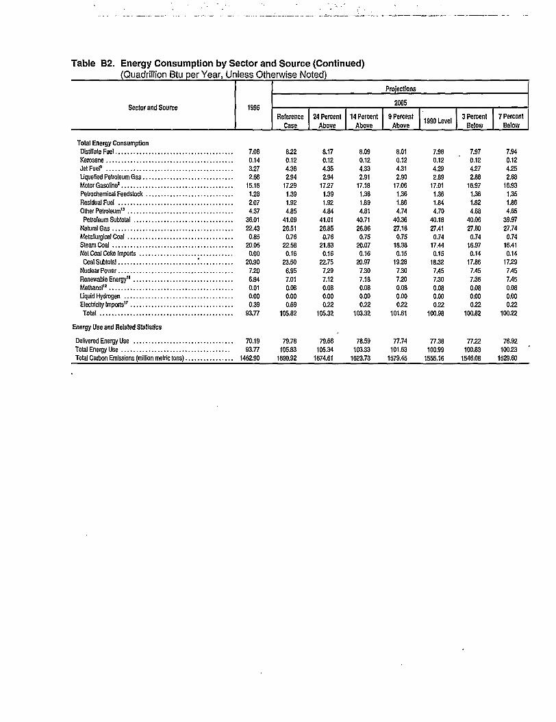
Table B2. Energy Consumption by Sector and Source (Continued)(Quadrillion Btu per Year, Unless Otherwise Noted)
Sector and Source 1S96
Projections
2005
Reference
Case
24 Percent
Above
14 Percent
Above
9 Percent
Above1990 Level
3 Percent
Below
7 Percent
Below
Total Energy Consumption
Distillate Fuel 7.06
Kerosene 0.14
JetFuel9 3.27
Liquefied Petroleum Gas 2.66
Motor Gasoline2 15.16
Petrochemical Feedstock 1.28
ResidualFuel 2.07
Other Petroleum" 4.37
Petroleum Subtotal 36.01
Natural Gas 22.43
Metallurgical Coal 0.85
SteamCoal 20.05
Net Coal Coke Imports 0.00
Coal Subtotal ! 20.90
NuclearPower 7.20
Renewable Energy" 6.84
Methanol" 0.01
Liquid Hydrogen 0.00
Electricity Imports" 0.39
Total 93.77
Energy Use and Related Statistics
Delivered Energy Use 70.19
Total Energy Use 93.77
Total Carbon Emissions (million metric tons) 1462.90
8.22
0.12
4.36
2.94
17.29
1.39
1.92
4.85
41.09
26.51
0.76
22.58
0.16
23.50
6.95
7.01
0.08
0.00
0.69
105.82
79.78
105.83
1690.92
8.17
0.12
4.35
2.94
17.27
1.39
1.92
4.84
41.01
26.85
0.76
21.83
0.16
22.75
7.29
7.12
0.08
0.00
0.22
105.32
79.66
105.34
1674.61
8.09
0.12
4.33
2.91
17.18
1.38
1.89
4.81
40.71
26.86
0.75
20.07
0.16
20.97
7.30
7.18
0.08
0.00
0.22
103.32
78.59
103.33
1623.73
8.01
0.12
4.31
2.90
17.06
1.36
1.86
4.74
40.36
27.18
0.75
18.38
0.15
19.28
7.30
7.20
0.08
0.00
0.22
101.61
77.74
101.63
1579.45
7.98
0.12
4.29
2.89
17.01
1.36
1.84
4.70
40.18
27.41
0.74
17.44
0.15
18.32
7.45
7.30
0.08
0.00
0.22
100.93
77.38
100.99
1555.16
7.97
0.12
4.27
2.88
16.97
1.36
1.82
4.68
40.06
27.80
0.74
16.97
0.14
17.88
7.45
7.36
0.08
0.00
0.22
100.82
77.22
100.83
1546.08
7.94
0.12
4.25
2.88
16.93
1.35
1.86
4.65
39.97
27.74
0.74
16.41
0.14
17.29
7.45
7.45
0.08
0.00
0.22
100.22
76.92
100.23
1529.60

Table B2. Energy Consumption by Sector and Source (Continued)(Quadrillion Btu per Year, Unless Otherwise Noted)
Projections
2010
Reference
Case
8.62
0.12
4.98
3.18
18.30
1.48
2.03
5.11
43,8228.97
0.70
23.24
0.20
24.146.17
7.27
0.14
0.000.66
111.18
84.63111.19
1790.62
24 Percent
Above
8.42
0.12
4,91
3.13
17.83
1.45
1.99
4.99
42.8329.57
0.65
18.83
0.22
19.70
6.68
7.44
0.15
0.00
0.10
106.48
82.28
106.491667.93
14 Percent
Above
8.24
0,11
4.75
3.09
17.16
1.42
1.94
4.92
41.6430.65
0.61
13.97
0,23
14.81
6.90
7.61
0.14
0.000.10
101.86
79.94101.87
1535.00
9 Percent
Above
8.17
0.11
4.68
3.08
16.81
1.41
1.94
4.91
41.12. 31.82
0.61
10.85
0.23
11.68
6.98
7.72
0.14
0.00
0.10
99.57
78.9099.58
1461.50
1990 Level
7.96
0.11
4.43
3.03
15.96
1.37
1.92
4.72
39.4932.38
0.60
6.98
0.22
7.80
7.36
7.98
0.14
0.000.10
95.23
75.83
95.25
1339.98
3 Percent
Below
7.94
0.11
4.32
3.02
15.58
1.36
1.96
4.61
38.8932.49
0.60
5.91
0.22
6.72
7.36
8.23
0.13
0.000.10
93.93
74.6693.94
1299.97
7 Percent
Below
7.87
0.11
4.18
3.03
14.97
1.35
2.05
4.50
38.0632.09
0.59
4.63
0.22
5.44
7.41
8.44
0.13
0.00
0.10
91.67
72.8791.68
1243.42
2020
Reference
Case
8.98
0.12
5.93
3.36
19.31
1.52
2.24
5.4246.8832.65
0.58
24.42
0.27
25.27
3.80
7.59
0.22
0.000.61
117.02
90.21117.01
1928.74
24 Percent
Above
8.65 '
0.11
5.78
3.28
18.36
1.46
2.19
5.4245.253450
0.44
14.52
0.32
15.28
5.06
8.29
0.22
0.00
0.04
108.64
86.30108.64
1668.05
14 Percent
Above
8.56
0.11
5.73
3.28
18.03
1.45
2.18
5.5344.8735.40
0.41
9.29
0.33
10.02
5.63
9.43
0.22
0.00
0.04
105.61
84.96
105.60
1536.23
9 Percent
Above
8.76
0.11
5.68
3.27
17.76
1.44
2.27
5.5044.7836.02
0.40
6.33
0.33
7.06
5.90
9.77
0.21
0.000.04
103.79
84.04103.79
1467.78
1990 Level
8.86
0.11
5.54
3.28
16.93
1.42
2.25
5.3643.7535.84
0.39
2.61
0.34
3.34
6.67
11.05
0.21
0.00
0.04
100.90
81.87
100.89
1346.70
3 Percent
Below
8.66
0.11
5.48
3.26
16.49
1.42
2.23
5.2942.943559
0.38
1.87
0.34
2.59
6.86
11.91
0.20
0.00
0.04
99.94
80.77
99.93
1303.26
7 Percent
Below
8.34
0.10
5.35
3.21
15.87
1.41
2.23
5.1641.673454
0.38
1.26
0.34
1.98
7.41
12.92
0.20
0.00
0.04
98.76
79.25
98.75
1250.80
'Includes wood used (or residential heating. See Table B18 estimates of nonmarketed renewable energy consumption for geothemal heat pumps & solar thermal hot water heating.'Includes ethanol (blends of 10 percent or less) and ethers blended into gasoline.'Includes commercial sector electricity cogenerated by using wood and wood waste, landfill gas, municipal solid waste, and other biomass. See Table B18 for estimates of nonmarketed
renewable energy consumption for solar thermal hot water heating.4Fuel consumption Includes consumption for cogeneration.'Includes petroleum coke, asphalt, road oil, lubricants, still gas, and miscellaneous petroleum products.'Includes lease and plant fuel.'Includes consumption of energy from hydroelectric, wood & wood waste,.municipal solid v/aste, & other biomass; includes for cogeneration, both sales to the grid & for own use.'Low sulfur dlesel fuel."Includes naphtha and kerosene type."Includes aviation gas and lubricants."E85 Is 85 percent ethanol (renewable) and 15 percent motor gasoline(nonrenewable)."Only M85 (85 percent methanol and 15 percent motor gasoline)."Includes unfinished oils, natural gasoline, motor gasoline blending compounds, aviation gasoline, lubricants, still gas, asphalt, road oil, petroleum coke, and miscellaneous petroleum
products.
"Includes electricity generated for sale to the grid and for own use from renev/able sources, and non-electric energy from renewable sources. Excludes nonmarketed renewable energy
consumption for geolhernial heat pumps and solar thermal hot water heaters."Includes consumption of energy by all electric power generators for grid-connected power except cogenerators, which produce electricity and other useful thermal energy."Includes conventional hydroelectric, geolhermal, wood and wood waste, municipal solid v/aste, other biomass, E85, wind, photovoltaic and solar thermal sources. Excludes cogeneration.
Excludes net electricity Imports." I n 1996 approximately two-thirds of the U.S. electricity imports were provided by renewable sources (hydroeiectricity); EIA does not project future proportions."Includes hydroelectric, geothermal, wood and v/ood v/aste, municipal solid waste, other biomass, wind, photovoltaic and solar thermal sources. Includes ethanol components of E85;
excludes elhanol blends (10 percent or less) In motor gasoline. Excludes net electricity imports and nonmarketed renev/able energy consumption for geothermal heat pumps and solar thermalhot water heaters.
Btu = British thermal unit.Note: Totals may not equal sum of components due to independent rounding. Figures for 1996 may differ from published data due to internal conversion factors. Consumption values of
0.00 are values that round to 0.00, because they are less than 0.005.Sources: 1996 natural gas lease, plant, and pipeline fuel values: Energy Information Administration, Short-Teim Energy Outlook, August 1997. Online. http:ZAvww.eia.doe.gov/emeu/steo
/puh/upd/aug97/index.html (August 21,1997). 1996 electric utility fuel consumption: EIA, Electric Power Annual 1996, Volume I, DOE/EIA-0348(96)/1 (Washington, DC, August 1997). 1996nonutility consumption estimates: EIA Form 867, "Annual Nonutility Power Producer Report." Other 1996 values: EIA, Short-Term Energy Outlook August 1997. Online.http://wwv,eia.dO9.gov/erneu/steo/pub/upd/aug97/index.html (August 21,1997). Projections: EIA, AEO98 National Energy Modeling System runs KYBASE.D080398A, FD24ABV.D080398B,FD1998.D080398B, FD09ABV.D080398B, FD1990.D080398B, FD03BLW.D080398B, and FD07BLW.D080398B.
Energy Information Administration / ImDacts of the Kvntn Prntnrni n n i i s Pn»n« Mari«»»e <,„,! i r — — : - A _.:..«..

Table B3. Energy Prices by Sector and Source(1996 Dollars per Million Btu)
Sector and Source1996
Projections
2005
Reference
Case
24 Percent
Above
14 Percent
Above
9 Percent
Above1990 Level
3 Percent
Below
7 Percent
Below
Residential 12.86
Primary Energy1 6.63Petroleum Products2 8.51
Distillate Fuel 7.09
Liquefied Petroleum Gas 11.59Natural Gas 6.19
Electricity 24.42
Commercial 12.84
Primary Energy1 5.26
Petroleum Products2 5.56
Distillate Fuel 5.27
Residual Fuel 3.24
NaturalGas3 5.28
Electricity 22.05
Industrial' 5.35Primary Energy 3.99
Petroleum Products2 5.58
Distillate Fuel 5.50
Liquefied Petroleum Gas 7.80
Residual Fuel 2.99
NaturalGas5 2.96
Metallurgical Coal 1.77
Steam Coal 1.46Electricity 13.37
Transportation 8.77
Primary Energy 8.76
Petroleum Products2 8.76
Distillate Fuel6 8.90
JetFuel7 5.52
Motor Gasoline' 9.89
Residual Fuel 2.55
Liquid Petroleum Gas9 12.63
Natural Gast0 5.42
E85" 15.85
M8512 12.24Electricity 15.33
Average End-Use Energy 8.65
Primary Energy 8.32
Electricity 20.00
Electric Generators"
Fossil Fuel Average 1.54
Petroleum Products 3.25Distillate Fuel 4.91
Residual Fuel • 3.07
Natural Gas 2.64
SteamCoal 1.29
12.18
6.26
9.187.59
12.115.63
21.55
11.62
4.81
5.76
5.37
3.07
4.73
19.21
4.96
3.75
5.21
5.43
6.70
2.75
2.80
1.63
1.30
11.57
8.62
8.61
8.61
8.47
5.37
9.92
2.70
12.99
5.82
16.35
12.54
13.44
8.21
7.92
17.49
1.50
3.44
4.97
3.10
2.62
1.17
12.37
6.33
9.287.68
12.235.69
21.95
11.84
4.88
5.86
5.46
3.204.79
19.62
5.07
3.83
5.28
5.53.
6.83
2.84
2.88
1.76
1.42
11.83
8.78
8.77
8.76
8.62
5.51
10.10
2.80
13.10
5.88
16.38
12.60
13.56
8.36
8.07
17.85
1.62
3.38
5.10
3.15
2.69
1.28
13.85
7.04
10.048.48
12.876.37
24.60
13.49
5.58
6.68
6.27
4.13
5.46
22.29
5.86
4.48
5.78
6.35
7.45
3.77
3.51
2.88
2.56
13.41
9.53
9.52
9.52
9.41
6.30
10.83
3.72
13.74
6.52
16.60
13.32
13.69
9.32
8.97
20.11
2.66
4.33
5.93
4.11
3.32
2.42
14.92
7.52
10.519.00
13.226.85
26.62
14.68
6.07
7.19
6.79
4.67
5.93
24.28
6.37
4.88
6.09
6.87
7.80
4.34
3.93
3.60
3.27
14.61
10.03
10.02
10.02
9.89
6.79
11.35
4.30
14.07
6.98
16.69
13.78
13.93
9.97
9.57
21.82
3.32
4.91
6.45
4.71
3.74
3.13
15.40
7.72
10.709.20
13.39
7.05
27.54
15.21
6.27
7.38
6.984.89
6.13
25.19
6.59
5.04
6.21
7.05
7.97
4.55
4.12
3.86
3.54
15.14
10.22
10.21
. 10.21
10.07
6.97
11.55
4.50
14.24
7.17
16.73
13.96
14.09
10.24
. 9.82
22.60
3.59
5.15
6.65
4.95
3.99
3.39
15.54
7.84
10.859.35
13.527.16
27.70
15.38
6.39
7.54
7.14
5.06
6.24
25.37
6.70
5.15
6.31
7.22
8.10
4.72
4.22
4.06
3.74
15.25
10.37
10.36
10.37
10.23
7.11
11.69
4.68
14.37
7.27
16.75
14.09
14.07
10.38
9.96
22.76
3.77
5.33
6.81
5.12
4.07
3.60
15.84
7.99
11.019.52
13.667.31
28.21
15.72
6.54
7.71
7.31
5.24. 6.39
25.89
6.85
5.28
6.41
7.38
8.24
4.90
4.36
4.28
3.96
15.56
10.53
10.52
10.52
10.39
7.26
11.85
4.84
14.50
7.41
16.78
14.23
14.06
10.56
10.13
23.20
3.97
5.47
6.98
5.29
4.24
3.81
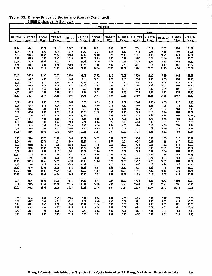
Table B3. Energy Prices by Sector and Source (Continued)(1996 Dollars per Million Btu)
Projections
2010
Reference
Case
12.24
6.24
9.54
7.78
12.50
5.56
21,36
11.514,745.99
5.57
3,18
4,6118.87
5.12
3.96
5.46
5.68
7.01
2.94
2.98
1.58
1.26
11.28
8.75
8.74
8.73
8,49
5.62
10,12
2.90
13.18
6.53
16.73
12.63
13.27
8.31
8,04
17,22
1.55
3.675.21
3.29
2,82
1.11
24 Percent
Above
14.61
7.32
10.54
8.86
13.29
6.64
25.63
14.16
5.827.076.65
4.43
5.67
23,21
6.26
4.86
6.05
6.76
7.79
4.17
3.96
3,28
2.96
13.86
9.84
9.83
9.82
9.58
6.69
11.25
4.16
13.95
7.60
16.79
13.54
13.78
9.76
9.38
20,92
3.144.876,35
4.63
3.81
2.81
14 Percent
Above
16.79
8.50
11.47
9.93
13.91
7.86
29.11
16.57
7.028.117.72
5.62
6,88
26.77
7.32
5.75
6.60
7.83
8.41
5.35
5.06
4.85
4.53
15.96
10.77
10.76
10.75
10.67
7.65
12.14
5.34
14.55
8.74
16.38
14.31
14.08
11.04
10.54
23,94
4.656,097.47
5,88
4.99
4.37
9 Percent
Above
18.11
9.18
11.94
10.47
14.27
8.58
31.29
17.99
7.718.648.26
6.26
7.60
28.85
7.92
6,26
6.87
8.35
8.76
5.96
5.74
5.69
5.37
17.12
11.22
11.21
11.20
11.18
8.15
12.55
5.96
14.89
9.39
16.39
14.71
14.74
11.73
11.16
25.70
5.496.718.03
6.52
5.70
5.23
1QQn I avallysu Level
20.87
10.79
13.39
12.10
15.34
10.20
35.46
21.05
9.3610.22
9.87
8.10
9.24
32.94
9.35
7.55
7.79
9.93
9.85
7.73
7.26
7.98
7.65
19.50
12.60
12.59
12.58
12.66
9.61
13.87
7.72
15.93
10.93
18.13
16.01
15.45
13.45
12.75
29.23
7.388.52
9.55
8.35
7.28
7.53
3 Percent
Below
21.94
11.39
14.07
12.83
15.93
10.78
37.17
22.31
9.99
10.95
10.60
8.90
9.83
34.71
9.95
8.09
8.25
10.66
10.44
8.56
7.81
8.98
8.65
20.51
13.24
13.24
13.23
13.37
10.24
14.50
8.54
16.52
11.49
18.83
16.60
15.80
14.18
13.44
30.68
8.049.34
10.14
9.11
7.80
8.55
7 Percent
Below
23.29
• 12.27
15.03
13.85
16.79
11.65
38.98
23.82
10.91
11.98
11.62
10.02
10.72
36.43
10.79
8.90
8.95
11.70
11.37
9.65
8.65
10.36
10.03
21.51
14.19
14.18
14.18
14.39
11.20
15.44
9.66
17.36
12.32
19.61
17.21
15.91
15.17
14.38
32.19
8.9610.48
11.14
10.24
8.63
9.95
2020
Reference
Case
12.32
6.42
9.72
7.82
12.49
. 5.80
20.37
11.104.70
6.12
5.66
3.38
4.57
17.67
5.15
4.16
5.58
5.86
6.99
3.16
3.25
1.51
1.18
10.31
8.59
8.57
8.55
8.22
5.76
10.01
3.08
12.76
7.17
16.58
12.69
12.39
8.27
7.98
16.31
1.684.035.36
3.56
3.20
1.00
24 Percent
Above
16.06
8.32
11.19
9.44
13.61 .
7.76
26.37
15.07
6.607.70
7.24
5.23
6.49
23.61
6.92
5.62
6.41
7.40
8.12
4.97
5.06
4.00
3.67
13.83
10.05
10.04
10.02
9.75
7.32
11.46
4.92
13.88
8.95
1650
13.86
12.77
10.39
9.90
21.44
4.225.94
6.99
5.67
4.97
3.48
14 Percent
Above
17.31
9.12
11.51
9.87
13.73
8.64
28.01
16.30
7.39
8.07
7.64
5.69
7.35
25.09
7.44
6.09
6.55
7.76
8.18
5.39
5.86
4.60
4.27
14.74
10.36
10.35
10.32
10.10
7.70
11.74
5.36
14.02
9.67
1627
14.14
12.90
10.98
10.40
22.79
5.206.71
7.21
6.245.81
4.07
9 PercentAbove
18.149.61
11.83102113.999.16
29.20
17.16
7.888.40
7.98
6.06
7.87
26.21
7 .83-
6.44
6.75
8.10
8.47
5.74
6.35
5.05
4.72
15.38
10.67
10.66
10.63
10.42
8.01
12.05
5.70
14.27
10.15
16.54
14.42
13.15
11.43
10.80
23.77
5.907.36
7.52
6.72
6.31
4.52
1QGn I QUAII99U Level
19.68
10.56
12.79
11.24
14.83
10.10
31.23
18.76
8.869.43
9.02
7.21
8.82
28.18
8.69
7.25
7.39
9.14
9.36
6.85
7.24
6.55
6.19
16.52
11.56
11.55
11.52
11.50
9.04
12.88
6.85
15.09
10.99
17.43
15.18
13.38
12.45
11.75
25.49
7.178.50
8.55
8.06
7.21
6.04
3 Percent
Below
20.34
11.06
13.43
11.90
15.42
10.57
31.94
19.459.39
10.12
9.68
8.01
9.30
28.85
9.17
7.73
7.80
9.80
9.95
7.63
7.71
7.56
72017.00
12.17
12.17
12.14
12.18
9.66
13.49
7.63
15.66
11.44
17.92
15.76
13.15
13.02
12.31
26.10
7.709.169.21
8.84
7.68
7.10
7 Percent
Below
21.52
11.91
14.51
13.06
16.39
11.37
33.34
20.6910.2811.30
10.85
9.33
10.12
30.13
9.93
8.52
8.49
10.97
10.87 .
8.91
8.50
9.19
8.83
17.67
13.22
13.22
13.20
13.34
10.73
14.53
8.96
16.61
12.20
19.09
16.74
13.27
13.98
13.24
27.21
8.5210.28
10.38
10.06
8.48
8.80
Energy Information Administration / Impacts of the Kyoto Protocol on U.S. Energy Markets and Economic Activity 169
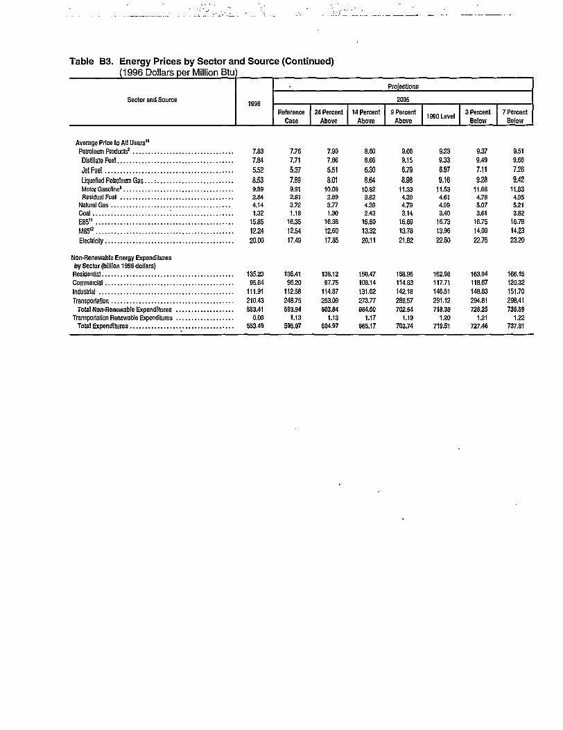
Table B3. Energy Prices by Sector ai(1996 Dollars per Million Btu
Sector and Source
id Source (Continued)
1996
Projections
2005
Reference
Case
24 Percent
Above
14 Percent
Above
9 Percent
Above1990 Level
3 Percent
Below
7 Percent
Below
Average Price to All Users"
Petroleum Products2 7.83
Distillate Fuel 7.84
Jet Fuel 5.52Liquefied Petroleum G a s . . . : 8.53Motor Gasoline* 9.89
Residual Fuel 2.84
Natural Gas 4.14
Coal i 1.32E85" 15.85
M85'2 12.24
Electricity 20.00
Non-Renewable Energy Expenditures
by Sector (billion 1996 dollars)
Residential 135.23
Commercial 95.84Industrial 111.91
Transportation 210.43
Total Non-Renewable Expenditures 553.41Transportation Renewable Expenditures 0.08
Total Expenditures 553.49
7.76
7.71
5.37
7.899.912.813.72
1.18
16.35
12.54
17.49
136.41
96.20
112.58
248.75
593.94
1.13
595.07
7.90
7.86
5.518.01
10.082.893.77
1.30
16.38
12.60
17.85
138.12
97.75
114.87
253.09
603.84
1.13
604.97
8.60
8.66
6.308.64
10.823.82
4.39
2.43
16.60
13.32
20.11
150.47
108.14
131.62
273.77
664.00
1.17
665.17
9.06
9.15
6.798.98
11.334.394.79
3.14
16.69
13.78
21.82
158.96
114.83
142.18
286.57
702.541.19
703.74
9.23
9.33
6.979.16
11.534.614.99
3.40
16.73
13.96
22.60
162.96
117.71
146.51
291.12
718.30
1.20
719.51
9.37
9.49
7.119.28
11.684.785.07
3.61
16.75
14.09
22.76
163.94
118.67
148.83
294.81
726.25
1.21
727.46
9.51
9.66
7.269.42
11.834.955.213.82
16.78
14.23
23.20
166.15
120.32
151.70
298.41
736.591.22
737.81

Table B3. Energy Prices by Sector and Source (Continued)(1996 Dollars per Million Btu)
Projections
2010
Reference
Case
7.94
7.81
5.62
8.29
10.11
2.98
3.76
1.12
16.73
12.63
17.22
142.47
100.04
121,43
273,12
637.05
1.97
639.03
24 Percent
Above
8.91
8.91
6,69
9.05
11.23
4.24
4.71
2.82
16.79
13.54
20.92
162.27
116.91
145.88
301.43
726.49
2.01
728.51
14 Percent
Above
9.74
9.99
7.65
9.67
12.12
5.42
5.80
4.39
16.38
14.31
23.94
178.46
129.55
168.16
320.24
796.40
2.04
798.44
9 Percent
Above
10.14
10.50
8.15
10.00
12.53
6.04
6.45
5.24
16.39
14.71
25.70
187.98
136.02
181.59
328.53
834.12
2.07
836.18
4QQA 1 atta\issU Level
11.39
12.01
9.61
11.07
13.86
7.81
7.96
7.56
18.13
16.01
29.23
206.89
147.66
209.59
353.51
917.65
2.12
919.77
3 Percent
Below
11.98
12.71
10.24
11.64
14.49
8.64
8.49
8.57
18.83
16.60
' 30.68
213.60
151.70
222.20
364.91
952.41
2.15
954.56
7 Percent
Below
12.83
13.72
11.20
12.52
15.43
9.76
9.31
9.97
19.61
17.21
32.19
221.60
155.24
238.74
379.60
995.18
2.18
997.35
Reference
Case
7.88
7.67
5.76
8.32
10.00
3.15
3.96
1.01
16.58
12.69
16.31
154.21
101.88
125.47
292.00
673.57
2.81
676.38
24 Percent
Above
9.18
9.21
7.32
9.44
11.45
4.99
5.69
3.50
16.20
13.86
21.44
186.09
126.71
164.58
329.71
807.09
2.86
809.95
14 Percent
' Above
9.43
9.54
7.70
9.52
11.73
5.43
6.48
4.10
16.27
14.14
22.79
194.97
132.32
176.32
334.53
838.14
2.91 •841.05
2020
9 Percent
Above
9.69
9.79
8.01
9.80
12.04
5.77
6.95
4.57
16.54
14.42
23.77
200.87
136.19
184.55
340.63
86223
£93865.16
"tOOn 1 awalissU Level
10.49
10.78
9.04
10.62
12.86
6.91
7.84
6.12
17.43
15.18
25.49
211.16
142.68
203.62
357.11
914.57
2.92
917.49
3 Percent
Below
11.06
11.49
9.66
11.19
13.48
7.70
8.30
7.18
17.92
15.76
26.10
215.46
144.77
214.30
370.26
' 944.78
2.94
947.72
7 Percent
Below
12.02
12.73
10.73
12.11
14.51
9.02
9.09
8.84
19.09
16.74
27.21
223.12
148.56
231.62
392.18
995.49
3.02
998.51
'Weighted average price includes fuels below as well as coal.'This quantity is the weighted average for all petroleum products, not just those listed below.'Excludes independent power producers.'Includes cogenerators.'Excludes uses for lease and plant fuel."Low sulfur diesel fuel. Price includes Federal and State taxes while excluding county and local taxes.7Kerosene-type jet fuel. Price includes Federal and State taxes while excluding county and local taxes.
'Sales weighted-average price for all grades. Includes Federal and State taxes and excludes county and local taxes.
'Includes Federal and State taxes while excluding county and local taxes."Compressed natural gas used as a vehicle fuel. Price includes estimated motor vehicle fuel taxes.11E85 is 85 percent ethanol (renev/able) and 15 percent motor gasoline (nonrenewable)."Only M85 (85 percent methanot and 15 percent motor gasoline)."Includes all electric power generators except cogenerators, which produce electricity and other useful thermal energy."Weighted averages of end-use fuel prices are derived from the prices shown in each sector and the corresponding sectoral consumption.Btu = British thermal unit.Note: 1996 figures may differ from published data due to internal rounding.Sources: 1996 prices for gasoline, distillate, and jet fuel are based on prices in various issues of Energy Information Administration (EIA), Petroleum Marketing Monthly, DOE/EIA-
0380(96/13-97/4) (Washington, DC, 1996-97). 1996 prices for all other petroleum products are derived from the EIA, State Energy Price and Expenditure Report 1994, DOE/EIA-0376(94)(Washington, DC, June 1997). 1996 industrial gas delivered prices are based on EIA, Manufacturing Energy Consumption Survey 1991.1996 residential and commercial natural gas deliveredprices: EIA, Natural Gas Monthly, DOE/EIA-0130(97/6) (Washington, DC, June 1997). Other 1996 natural gas delivered prices: EIA, AEO98 National Energy Modeling System runsKYBASE.D080398A, FD24ABV.D080398B, FD1998.D080398B, FD09ABV.D080398B, FD1990.D080398B, FD03BLW.D080398B, and FD07BLW.D080398B. Values for 1996 coal prices havebeen estimated from EIA, State Energy Price and Expenditure Report 1994, DOE/EIA-0376(94) (Washington, DC, June 1997) by use of consumption quantities aggregated from EIA, StareEnergy Data Report 1994. Online, ftp://ftp.eia.doe.gov/ pub/state.data/021494.pdf (August 26,1997) and the Coaf Industry Annual 1996, DOE/EIA-0584(96) (Washington, DC, November1997). 1996 electricity prices for commercial, industrial, and transportation: EIA, AEO98 National Energy Modeling System runs KYBASE.D080398A, FD24ABV.D080398B, FD1998.D080398B,FD09ABV.D080398B, FD1990.D080398B, FD03BLW.D080398B, and FD07BLW.D080398B. Projections: EIA, AEO98 National Energy Modeling System runs KYBASE.D080398A,FD24ABV.D080398B, FD1998.D080398B, FD09ABV.D080398B, FD1990.D080398B, FD03BLW.D080398B, and FD07BLW.D080398B.
Energy Information Administration / Impacts of the Kyoto Protocol on U.S. Energy Markets and Economic Activity 171

Table B4. Residential Sector Key Indicators and End-Use Consumption(Quadrillion Btu per Year, Unless Otherwise Noted)
Key Indicators and Consumption 1996
Projections
2005
Reference
Case
24 Percent
Above
14 Percent
Above
9 Percent
Above1990 Level
3 Percent
Below
7 Percent
Below
Key Indicators
Households (millions)
Single-Family 69.61
Multifamily 24.76
Mobile Homes 6.00
Total 100.37
Average House Square Footage 1649
Energy Intensity
(million Btu consumed per household)
Delivered Energy Consumption 110.92Electricity Related Losses 81.78Total Energy Consumption 192.70
Delivered Energy Consumption by Fuel
Electricity
Space Heating
Space Cooling
Water Heating
Refrigeration
Cooking
Clothes Dryers
Freezers
Lighting
Clothes Washers1
Dishwashers'
Color Televisions
Personal Computers
Furnace Fans
Other Uses2
Delivered Energy
Natural Gas
Space Heating
Space CoolingWater Heating
Cooking
Clothes Dryers
Other Uses3
Delivered Energy
Distillate
Space Heating
WaterHeating
Other Uses4
Delivered Energy
Liquefied Petroleum Gas
Space Heating
WaterHeating
Cooking
Other Uses3
Delivered Energy
Marketed Renewables (wood)5
OtherFuels6 ,
77.46
26.54
7.08
111.08
77.46
26.54
7.08
111.08
77.43
26.52
7.08
111.02
77.40
26.50
7.07
110.97
77.3826.49
7.07
110.95
77.38
26.49
7.07
110.94
77.37
26.48
7.07
110.92
1691 1691 1691 1691 1691 1691 1691
106.3082.08
188.37
105.9780.85
186.82
103.3477.75
181.09
101.5075.07
176.57
100.8874.40
175.28
100.5974.35
174.93
100.0573.50
173.55
0.47
0.46
0.370.41
0.13
0.19
0.13
0.32
0.03
0.05
0.21
0.02
0.09
0.79
3.68
3.77
0.00
1.31
0.16
0.05
0.09
5.39
0.80
0.09
0.00
0.89
0.32
0.07
0.03
0.01
0.42
0.61
0.13
0.48
0.51
0.37
0.31
0.14
0.21
0.09
0.37
0.03
0.05
0.29
0.03
0.11
1.35
4.34
3.86
0.00
1.35
0.17
0.05
0.10
5.53
0.68
0.09
0.00
0.77
0.32
0.08
0.03
0.01
0.44
0.61
0.13
0.48
0.51
0.37
0.31
0.14
0.21
0.09
0.37
0.03
0.05
0.29
0.03
0.11
1.34
4.32
3.85
0.00
1.35
0.17
0.05
0.10
5.52
0.68
0.09
0.00
0.77
0.31
0.08
0.03
0.01
0.43
0.61
0.13
0.46
0.49
0.36
0.31
0.14
0.21
0.09
0.36
0.03
0.05
0.28
0.03
0.10
1.30
4.21
3.73
0.00
1.31
0.17
0.05
0.10
5.35
0.66
0.09
0.00
0.75
0.31
0.08
0.03
0.01
0.43
0.61
0.12
0.45
0.48
0.35
0.31
0.14
0.20
0.09
0.35
0.03
0.05
0.28
0.03
0.10
1.27
4.13
3.65
0.00
1.28
0.17
0.05 .
0.09
5.25
0.65
0.09
0.00
0.74
0.31
0.07
0.03
0.01
0.43
0.61
0.11
0.45
0.47
0.350.31
0.14
0.20
0.09
0.350.03
0.05
0.28
0.03
0.10
1.26
4.10
3.62
0.00
1.27
0.17
0.05
0.09
5.21
0.65
0.09
0.00
0.74
0.31
0.07
0.03
0.01
0.43
0.61
0.11
0.45
0.47
0.35
0.31
0.14
0.20
0.09
0.35
0.03
0.05
0.27
0.03
0.10
1.26
4.09
3.61
0.00
1.27
0.17
0.05
0.09
5.19
0.64
0.09
0.00
0.73
0.31
0.07
0.03
0.01
0.42
0.61
0.11
0.44
0.47
0.35
0.31
0.14
0.20
0.09
0.340.03
0.05
0.27
0.03
0.10
1.25
4.07
3.58
0.00
1.26
0.17
0.05
0.09
5.16
0.64
0.09
0.00
0.73
0.30
0.07
0.03
0.01
0.42
0.61
0.11

Table B4. Residential Sector Key Indicators and End-Use Consumption (Continued)(Quadrillion Btu per Year, Unless Otherwise Noted)
Projections
2010
Reference
Case
24 Percent
Above
14 Percent
Above
9 Percent
Above1990 Level
3 Percent
Below
7 Percent
Below
Projections
2020
Reference
Case
24 Percent
Above
14 Percent
Above
9 Percent
Above1990 Level
3 Percent
Below
7 Percent
Below
81.55
27.92
7.58
117.04
81.48
27.85
7.57
116.90
81.37
27.71
7.56
116.64
81.34
27.68
7.56
116.58
81.19
27.52
7.55
116.26
81.14
27.47
7.54
116.15
81.08
27.42
7.54
116.04
89.52
30.84
8.35
128.71
89.50
30.76
8.37
128.62
89.53
30.75
8.39
128.68
89.50
30.71
8.40
128.60
89.41
30.56
8.41
128.38
89.59
30.70
8.45
128.74
89.61
30.70
8.47
128.78
1707 1707 1707 1707 1708 1708 1708 1732 1732 1732 1732 1733 1732 1732
104.60
79.49
184.09
100.24
72.59
172.83
96.41
66.09
162.50
94.35
62.35
156.70
90.64
59.29
149.94
89.21
58.97
148.18
87.44
57.88
145.32
102.07
76.23
178.30
94.99
63.67
158.66
92.50
59.04
151.53
91.07
56.62
147.68
88.64
54.82
143.47
87.41
55.26
142.67
85.69
56.32
142.01
0.480,530,38
0.29
0.15
0.23
0,08
0.40
0,03
0.05
0,30
0.04
0.12
1.55
4.62
3,97
0,00
1.40
0,18
0,06
0,10
5,71
0,64
0.09
0.00
0.73
0,32
0,08
0,040,010.45
0.610,12
0.460,500.36
0.280.15
0,22
0.08
0.38
0.03
0,05
0.29
0,04
0.11
1.48
4.42
3.76
0.00
1.34
0.18
0.05
0.10
5.43
0.61
0.090.00
0.70
0.31
0.08
0.040.010.44
0.61
0.11
0.430.470.35
0.280.15
0.21
0.08
0.36
0.03
0.05
0.28
0.04
0.11
1.43
4.27
3.55
0.00
1.28
0.18
0.05
0.10
5.15
0.58
0.08
0.00
0.67
0.31
0.08
0.040.010.44
0.62
0.10
0.420.460.340.280.15
0.20
0.08
0.35
0.03
0.05
0.27
0.04
0.11
1.41
4.19
3.44
0.00
1.24
0.18
0.05
0.095.00
0.57
0.08
0.00
0.65
0.31
0.08
0.040.010.43
0.62
0.10
0.400.440.33
0.280.15
0.20
0.08
0.34
0.03
0.05
0.27
0.04
0.10
1.36
4.05
3.22
0.01
1.18
0.17
0.05
0.09
4.72
0.54
0.08
0.000.62
0.30
0.08
0.040.010.42
0.63
0.10
0.400.430.32
0.280.15
0.20
0.08
0.33
0.03
0.05
0.26
0.04
0.10
1.34
3.99
3.15
0.01
1.17
0.17
0.05
0.09
4.64
0.52
0.08
0.00
0.60
0.29
0.08
0.040.010.41
0.63
0.09
0.390.420.310.28
0.15
0.19
0.08
0.31
0.03
0.05
0.26
0.04
0.10
1.32
3.93
3.05
0.01
1.14
0.17
0.05
0.09
4.51
0.51
0.08
0.00
0.59
0.29
0.08
0.040.010.41
0.63
0.09
0.510.570.410.270.17
0.26
0.07
0.45
0.03
0.05
0.33
0.06
0.14
1.96
5.30
4.13
0.01
1.48
0.19
0.06
0.11
5.98
0.57
0.09
0.00
0.66
0.33
0.09
0.040.010.47
0.62
0.12
0.470.520.380.270.17
0.24
0.07
0.42
0.03
0.05
0.31
0.06
0.13
•1.84
4.97
3.74
0.01
1.35
0.19
0.06
0.11
5.45
0.53
0.08
0.00
0.61
0.32
0.09
0.040.010.46
0.63
0.10
0.460.500.370.270.17
0.24
0.07
0.41
0.03
0.05
0.31
0.05
0.13
1.81
4.88
3.57
0.01
1.29
0.19
0.06
0.105.22
0.51
0.08
0.00
0.60
0.32
0.09
0.040.010.46
0.64
0.10
0.450.490.370.270.17
0.23
0.07
0.41
0.03
0.05
0.31
0.05
0.13
1.79
4.82
3.47
0.01
1.27
0.19
0.06
0.10
5.10
0.51
0.08
0.00
0.59
0.32 .
0.09
0.040.010.46
0.64
0.10
0.440.470.360.270.17
0.23
0.07
0.40
0.03
0.05
0.30
0.05
0.13
1.76
4.73
3.31
0.01
1220.19
0.05
0.10
4.89
0.48
0.08
0.00
0.56
0.31
0.09
0.040.010.45
0.65
0.09
0.440.470.350.270.17
0.23
0.07
0.39
0.03
0.05
0.30
0.05
0.12
1.75
4.71
3.25
0.01
1.21
0.19
0.05'
0.10
4.81
0.47
0.08
0.00
0.55
0.30
0.08
0.040.010.44
0.66
0.09
0.430.460.340.27
0.17
0.23
0.07
0.39
0.03
0.05
0.30
0.05
0.12
1.73
4.65
3.15
0.01
1.18
0.19
0.05
0.104.68
0.45
0.08
0.00
0.53
0.29
0.080.040.010.42
0.67
0.09
Energy Information Administration / Impacts of the Kyoto Protocol on U.S. Energy Markets and Economic Activity 173
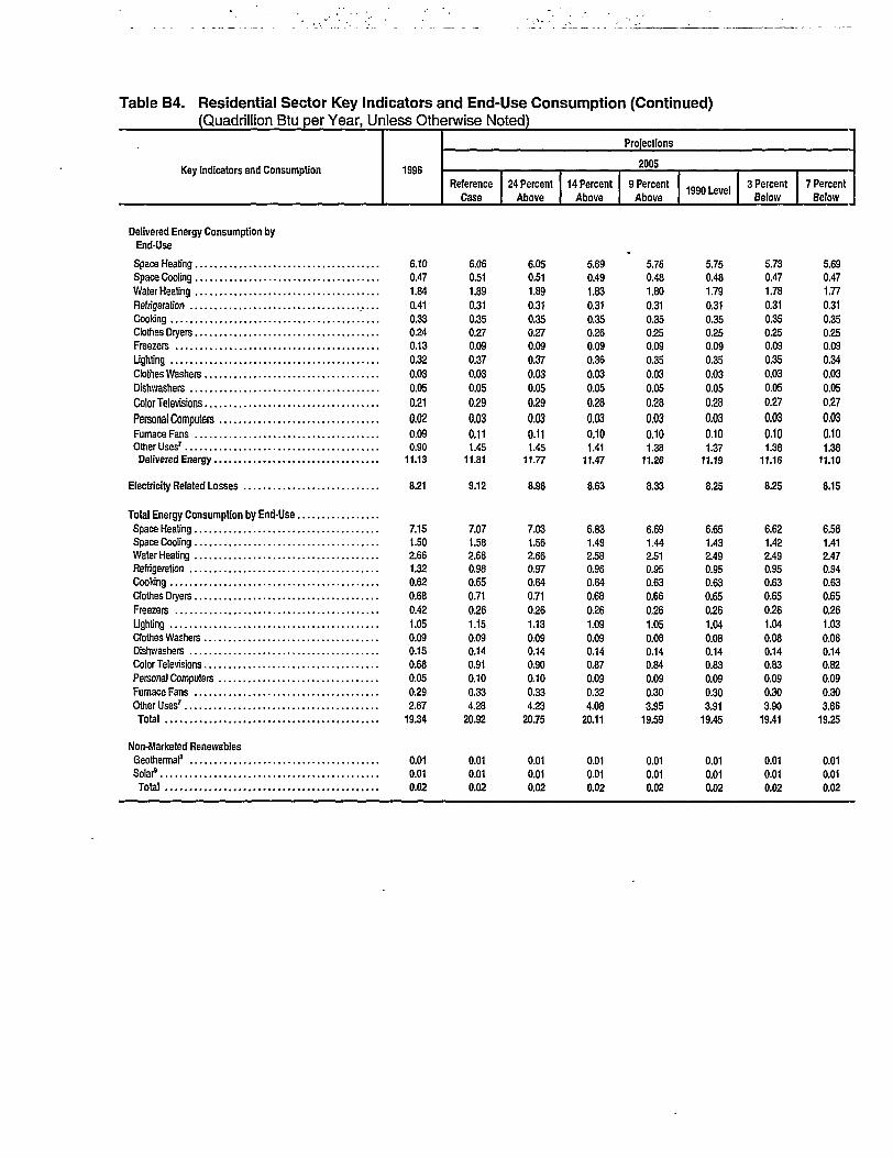
Table B4. Residential Sector Key Indicators and End-Use Consumption (Continued)(Quadrillion Btu per Year, Unless Otherwise Noted)
Key Indicators and Consumption 1996
Reference
Case
24 Percent
Above
14 Percent
Above
Proiections
2005
9 Percent
Above1990 Level
3 Percent
Below
7 Percent
Below
Delivered Energy Consumption by
End-Use
Space Heating 6.10
Space Cooling 0.47
WaterHeating 1.84
Refrigeration 0.41
Cooking 0.33
Clothes Dryers 0.24
Freezers 0.13
Lighting 0.32
Clothes Washers 0.03
Dishwashers 0.05
Color Televisions 0.21Personal Computers 0.02Furnace Fans 0.09OtherUses7 0.90
Delivered Energy 11.13
Electricity Related Losses 8.21
Total Energy Consumption by End-Use
Space Heating 7.15
Space Cooling 1.50
WaterHeating 2.66
Refrigeration 1.32
Cooking 0.62Clothes Dryers 0.68
Freezers 0.42
Lighting 1.05
Clothes Washers 0.09
Dishwashers 0.15
Color Televisions 0.68
Personal Computers 0.05
Furnace Fans 0.29
OtherUses7 2.67
Total 19.34
Non-Marketed Renewables
Geothermal8 0.01
Solar9 0.01
Total 0.02
6.06
0.51
1.89
0.31
0.35
0.27
0.09
0.37
0.03
0.05
0.290.030.111.45
11.81
6.05
0.51
1.89
0.31
0.35
0.27
0.09
0.37
0.03
0.05
0.290.030.111.45
11.77
5.89
0.49
1.83
0.31
0.35
0.26
0.09
0.36
0.03
0.05
0.280.030.101.41
11.47
5.78
0.48
1.80
0.31
0.35
0.25
0.09
0.35
0.03
0.05
0.28
0.030.101.38
11.26
5.75
0.48
1.79
0.31
0.35
0.25
0.09
0.35
0.03
0.05
0.28
0.030.101.37
11.19
5.73
0.47
1.78
0.31
0.35
0.25
0.09
0.35
0.03
0.05
0.27
0.030.101.36
11.16
5.69
0.47
1.77
0.31
0.35
0.25
0.09
0.34
0.03
0.05
0.270.030.101.36
11.10
9.12 8.S8 8.63 8.33 8.25 8.25 8.15
7.07
1.58
2.68
0.98
0.65
0.71
0.26
1.15
0.09
0.14
0.91
0.10
0.33
4.28
20.92
0.01
0.01
0.02
7.03
1.56
2.66
0.97
0.64
0.71
0.26
1.13
0.09
0.14
0.90
0.10
0.33
4.23
20.75
0.01
0.01
0.02
6.83
1.49
2.58
0.96
0.64
0.68
0.26
1.09
0.09
0.14
0.87
0.09
0.32
4.08
20.11
0.01
0.01
0.02
6.69
1.44
2.51
0.95
0.63
0.66
0.26
1.05
0.08
0.14
0.84
0.09
0.30
3.95
19.59
0.01
0.01
0.02
6.65
1.43
2.49
0.95
0.63
0.65
0.26
1.04
0.08
0.14
0.83
0.09
0.30
3.91
19.45
0.01
0.01
0.02
6.62
1.42
2.49
0.95
0.63
0.65
0.26
1.04
0.08
0.14
0.83
0.09
0.30
3.90
19.41
0.01
0.01
0.02
6.58
1.41
2.47
0.94
0.63
0.65
0.26
1.03
0.08
0.14
0.82
0.09
0.30
3.86
19.25
0.01
0.01
0.02

Table B4. Residential Sector Key Indicators and End-Use Consumption (Continued)(Quadrillion Btu per Year, Unless Otherwise Noted)
Projections
2010
Reference
Case
24 Percent
Above
14 Percent
Above
9 Percent
Above1990 Level
3 Percent
Below7 Percent
Below
Projections
2020
Reference
Case24 Percent
Above14 Percent
Above9 Percent
Above 1990 Level3 Percent
Below7 Percent
Below
6.140.54
1.96 '
0.29
0.36
0.28 .
0.08
0,40
0.03
0.05
0.30
0.04
0,12
1.67
12.24
5.86
0.50
1.87
0.28
0,36
0.27
0.08
0.38
0.03
0,05
0.29
0.04
0,11
1.59
11.72
5,59
0.48
1.79
0.28
0.36
0.26
0.08
0.36
0.03
0.05
0.28
0.04
0.11
1.54
11.25
5.45
0.46
1.75
0.28
0.36
0.26
0.08
0.35
0.03
0.05
0.27
0.04
0.11
1.51
11.00
5.18
0.44
1.67
0.28
0.36
0.25
0.08
0.34
0.03
0.05
0.27
0.04 •
0.10
1.46
10.54
5.09
0.43
1.64
0.28
0.36
0.24
0.08
0.33
0.03
0.05
0.26
0.04
0.10
1.44
10.36
4.96
0.42
1.61
0.28
0.36
0.24
0.08
0.31
0.03
0.05
0.26
0.04
0.10
1.42
10.15
6.28
0.58
2.06
0.27
0.40
0.32
0.07
0.45
0.03
0.05
0.33
0.06
0.14
2.09
13.14
5.78
0.53
1.90
0.27
0.40
0.30
0.07
0.42
0.03
0.05
0.31
0.06
0.13
1.96
12.22
5.60
0.51
1.84
0.27
0.40
0.29
0.07
0.41
0.03
0.05
0.31
0.05
0.13
1.93
11.90
5.49
0.50
1.81
0.27
0.40
0.29
0.07
0.41
0.03
0.05
0.31
0.05
0.13
1.91
11.71
5.29
0.48
1.75
. 0.27
0.40
0.29
0.07
0.40
0.03
0.05
0.30
0.05
0.13
1.87
11.38
5.21
0.48
1.72
0.27
0.40
0.28
0.07
0.39
0.03
0.05
0.30
0.05
0.12
1.87
11.25
5.08
0.47
1.68
0.27
0.40
0.28
0.07
0.39
0.03
0.05
0.30
0.05
0.12
1.84
11.04
9.30 8.49 7.71 7.27 6.89 6.85 6.72 9.81 8.19 7.60 7.28 7.04 7.11 7.25
7.11
1.60
2.72
0.86
0,67
0.74
0.23
1,200,090.140.910.120.36
4.79
21.55
0.02
0.01
0.03
6.74
1.46
2.56
0.83
0.65
0.68
0.22
1.10
0,09
0,140.840.12
0.33
4.44
20.20
0.02
0.01
0.03
6.37
1.33
2.42
0.80
0.63
0.64
0.21
1.02
0.080.13
0.780.11
0.31
4.12
18.95
0.02
0.010.03
6.18
1.26
2.34
0.78
0.62
0.61
0.21
0.97
0.080.13
0.750.100.29
3.95
18.27
0.02
0.01
0.03
5.87
1.18
2.22
0.76
0.62
0.58
0.20
0.91
0.080.130.720.100.28
3.78
17.43
0.02
0.01
0.03
5.77
1.16
2.19
0.77
0.62
0.58
0.20
0.88
0.080.130.710.10
0.28
3.74
17.21
0.02
0.01
0.03
5.63
1.14
2.14
0.77
0.62
0.57
0.20
0.85
0.080.130.700.100.27
3.69
16.86
0.02
0.01
0.03
7.23
1.63
2.82
0.78
0.71
0.80
0.21
1.28
0.090.150.960.17
0.40
5.72
22.95
0.04
0.010.05
6.55
1.38
2.53
0.72
0.68
0.70
0.19
1.110.090.140.830.15
0.35
4.99
20.41
0.04
0.01
0.05
6.31
1.29
2.42
0.70
0.66
0.66
0.18
1.05
0.080.140.790.14
0.33
4.74
19.50
0.04
0.01
0.05
6.17
1542.36
0.68
0.65
0.64
0.18
1.02
0.080.140.770.14
0.32
4.61
18.99
0.04
0.01
0.05
5.95
1.18
2.28
0.68
0.65
0.63
0.18
0.99
0.080.130.750.13
0.31
4.49
18.42
O.O4
0.01
0.05
5.87
1.18
2.25
0.69
0.65
0.63
0.18
0.99
0.080.140.750.13
0.31
4.52
18.37
0.05
O.010.06
5.75
1.18
2.22
0.70
0.66
0.63
0.18
0.990.080.140.760.13
0.31
4.55
1829
0.05
0.01
0.06
'Does not include water heating of load.'Includes small electric devices, heating elements and motors.'Includes such appliances as swimming pool heaters, outdoor grills, and outdoor lighting (natural gas).'Includes such appliances as swimming pool and hot tub heaters."Includes v/ood used for primary and secondary heating in wood stoves or fireplaces as reported in the Residential Energy Consumption Survey 1993.'Includes kerosene and coal.'Includes all other uses listed above.'Includes primary energy displaced by geothermai heat pumps in space heating and cooling applications."Includes primary energy displaced by solar thermal water heaters.Btu = British thermal unit.Note: Totals may not equal sum of components due to independent rounding.Sources: 1996; Energy Information Administration (EIA) Short-Term Energy Outlook, August 1997. Online, http://www.eia.doe.gov/emeu/steo/pub/upoyaug97/index.html (August 2 1 ,
1997). Projections: EIA, AEO98 National Energy Modeling System runs KYBASE.D080398A, FD24ABV.D080398B, FD1998.D080398B, FD09ABV.D080398B, FD1990.D080398B,FD03BLW.D080398B, and FD07BLW.D080398B.
Energy Information Administration / Impacts of the Kvoto Protocol on u s Frmrnu =»nri c™n,,m:~ A .

Table B5. Commercial Sector Key Indicators and End-Use Consumption(Quadrillion Btu per Year, Unless Otherwise Noted)
Key Indicators and Consumption 1996
Projections
2005
ReferenceCase
24 PercentAbove
14 PercentAbove
9 PercentAbove 1990 Level 3 Percent
Below7 Percent
Below
Key Indicators
Total Floor Space (billion square feet)
Surviving 69.2
New Additions 1.7
Total 70.9
Energy Consumption Intensity
(thousand Btu per square foot)
Delivered Energy Consumption 105.3
Electricity Related Losses 106.0
Total Energy Consumption 211.2
Delivered Energy Consumption by Fuel
ElectricitySpace Heating 0.12
Space Cooling 0.51WaterHeaBng 0.17
Ventilation 0.17
Cooking 0.03Lighting 1.16
Refrigeration 0.14Office Equipment (PC) 0.07Office Equipment (non-PC) 0.20Other Uses1 0.80
Delivered Energy 3.37
Natural Gas2
Space Heating 1.34
Space Cooling 0.02
WaterHeating 0.46
Cooking 0.18
OtherUses3 1.29
Delivered Energy 3.30
DistillateSpace Heating 0.20
WaterHeating 0.05
OtherUses4 0.19
Delivered Energy 0.44
Other Fuels5 0.36
Marketed Renewable Fuels
Biomass 0.00
Delivered Energy 0.00
Delivered Energy Consumption by End-Use
Space Heating 1.65Space Cooling 0.53WaterHeating 0.68
Ventilation 0.17
Cooking 0.21
Lighting 1.16
Refrigeration 0.14
Office Equipment (PC) 0.07
Office Equipment (non-PC) 0.20
OtherUses$ 2.64
Delivered Energy 7.47
77.3
1.7
79.0
104.8
104.2
209.0
77.3
1.7
79.0
104.5
102.6
207.2
77.3
1.7
79.0
101.5
98.4
199.9
77.3
1.7
79.0
99.0
94.5
193.5
77.3
1.7
79.0
98.0
93.2
191.2
77.3
1.7
79.0
97.7
' 93.3
191.0
77.3
1.7
79.0
96.9
92.0
188.9
0.11
0.54
0.17
0.18
0.031.250.150.080.251.15
3.91
1.38
0.03
0.50
0.21
1.52
3.63
0.17
0.05
0.17
0.39
0.11
0.54
0.17
0.18
0.031.240.150.080.251.14
3.90
1.37
0.03
0.49
0.21
1.52
3.62
0.17
0.050.17
0.39
0.11
0.52
0.17
0.18
0.03
1.21
0.150.080.24
1.12
3.80
1.33
0.03
0.48
0.20
1.47
3.51
0.16
0.05
0.16
0.37
0.10
0.51
0.16
0.17
0.03
1.17
0.15O.080.24
1.09
3.70
1.29
0.03
0.47
0.20
1.44
3.42
0.16
0.050.16
0.36
0.10
0.50
0.16
0.17
0.03
1.16
0.150.080.231.07
3.65
1.28
0.03
0.46
0.20
1.42
3.39
0.16
0.05
0.16
0.36
0.10
0.50
0.16
0.17
0.03
1.16
0.150.080.23
1.08
3.65
1.28
0.03
0.46
0.20
1.41
3.37
0.16
0.04
0.16
0.36
0.10
0.50
0.16
0.170.031.150.150.080.231.07
3.63
1.26
0.03
0.45
0.19
1.40
3.34
0.15
0.04
0.16
0.35
0.34 0.34 0.34 0.33 0.33 0.33 0.33
0.00
0.00
1.650.570.720.18
0.24
1.25
0.15
0.08
0.25
3.18
8.28
0.00
0.00
1.650.570.720.18
0.24
1.24
0.15
0.08
0.25
3.18
8.26
0.00
0.00
1.60
0.550.690.18
0.23
1.21
0.15
0.08
0.24
3.09
8.02
0.00
0.00
1.550.540.680.17
0.23
1.17
0.15
0.08
0.24
3.02
7.82
0.00
0.00
1.540.530.670.17
0.22
1.16
0.15
0.08
0.23
2.99
7.74
0.00
0.00
1.53
0.530.67
0.17
0.22
1.16
0.15
0.08
0.23
2.98
7.72
0.00
0.00
1.52
0.530.660.17
0.22
1.15
0.15
0.08
0.23
2.96
7.66
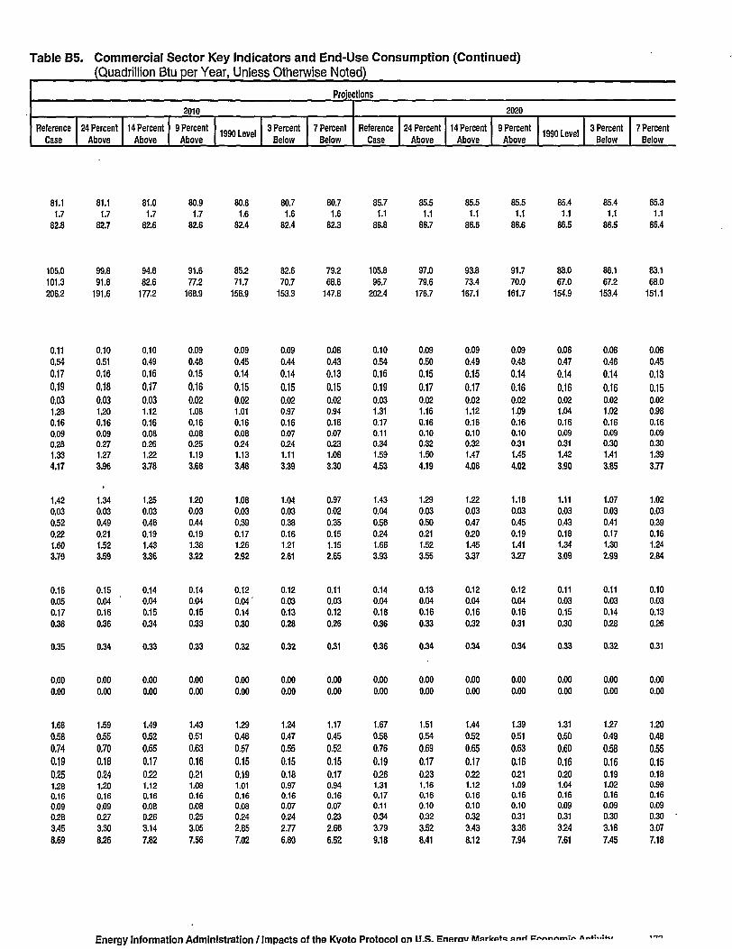
Table B5. Commercial Sector Key Indicators and End-Use Consumption (Continued)(Quadrillion Btu per Year, Unless Otherwise Noted)
Projections
2010
Reference
Case
24 Percent
Above
14 Percent
Above
9 Percent
Above1990 Level
3 Percent
Below
7 Percent
Below
2020
Reference
Case
24 Percent
Above
14 Percent
Above
9 Percent
Above1990 Level
3 Percent
Below
7 Percent
Below
81.1
1.7
82.8
105.0
101.3
206.2
81.1
1.7
82.7
99.8
91.8
191.6
81.0
1.7
82.6
94.6
82.6
177.2
80.9
1.7
82.6
91.6
77.2
168.9
80.8
1.6
82.4
85.2
71.7
156.9
80.7
1.6
82.4
82.6
70.7
153.3
80.7
1.6
82.3
79.2
68.6
147.8
85.7
1.1
86.8
105.8
96.7
202.4
85.5
1.1
86.7
97.0
79.6
176.7
85.5
1.1
86.6
93.8
73.4
167.1
85.5
1.1
86.6
91.7
70.0
161.7
85.4
1.1
86.5
88.0
67.0
154.9
85.4
1.1
86.5
86.1
67.2
153.4
85.3
1.1
86.4
83.1
68.0
151.1
0.11
0,54
0,170,190,031.28
0.16
0.090.28
1.33
4.17
1,42
0,03
0,52
0.22
1.60
3.79
0.16
0.05
0.17
0.38
0.10
0.51
0,16
0,180,031.20
0.160.090.27
1.27
3.96
1.34
0.03
0,49
0.21
1.52
3.59
0.15
0.04
0.16
0.36
0.10
0.49
0,16
0.170.031.12
0.160.080.261.22
3.78
1.25
0.03
0.46
0.19
1.43
3.36
0.14
0.04
0.15
0.34
0.09
0.48
0.15
0,160.021.08
0.160.080.25
1.19
3.68
1.20
0.03
0.44
0.19
1.38
3.22
0.14
0.04
0.15
0.33
0.09
0.45
0.14
0.150.02
1.01
0.160.080.24
1.13
3.48
1.08
0.03
0.39
0.17
1.26
2.92
0.12
0.04"
0.14
0.30
0.09
0.44
0.14
0.150.020.97
0.160.070.24
1.11
3.39
1.04
0.03
0.38
0.16
1.21
2.81
0.12
0.03
0.13
0.28
0.08
0.43
0.13
0.150.020.94
0.160.070.23
1.08
3.30
0.97
0.02
0.35
0.15
1.15
2.65
0.11
0.03
0.12
0.26
0.10
0.54
0.16
0.190.03
1.31
0.170.110.34
1.59
4.53
1.43
0.04
0.56
0.24
1.66
3.93
0.14
0.04
0.18
0.36
0.09
0.50
0.150.170.021.16
0.160.100.32
1.50
4.19
1.29
0.03
0.50
0.21
1.52
3.55
0.13
0.04
0.16
0.33
0.09
0.49
0.150.170.02
1.12
0.160.100.32
1.47
4.08
1.22
0.03
0.47
0.20
1.45
3.37
0.12
0.04
0.16
0.32
0.09
0.48
0.140.160.02
1.09
0.160.100.31
1.45
4.02
1.18
0.03
0.45
0.19
1.41
357
0.12
0.04
0.16
0.31
0.08
0.47
0.140.160.02
1.04
0.160.090.31
1.42
3.90
1.11
0.03
0.43
0.18
1.34
3.09
0.11
0.03
0.15
0.30
0.08
0.46
0.140.160.02
1.02
0.160.090.30
1.41
3.85
1.07
0.03
0.41
0.17
1.30
2.99
0.11
0.03
0.14
0.28
0.08
0.45
0.130.150.02
0.98
0.160.090.30
1.39
3.77
1.02
0.03
0.39
0.16
1.24
2.84
0.10
0.03
0.13
0.26
0.35 0.34 0.33 0.33 0.32 0.32 0.31 0.36 0.34 0.34 0.34 0.33 0.32 0.31
0,00
0.00
1.68
0,58
0,740,190,251.280.160,090.28
3,45
8.69
0.00
0.00
1.59
0.55
0,70
0,180,241.200.160.09
0.27
3.30
8.26
0.00
0.00
1.49
0.52
0.65
0.170.22
1.120.160.08
0.26
3.14
7.82
0.00
0.00
1.43
0.51
0.63
0,160.211.080.160.08
0.25
3.05
7.56
0.00
0.00
1.29
0.48
0.57
0.150.19
1.010.160.080.24
2.85
7.02
0.00
0.00
1.24
0.47
0.55
0.150.180.970.160.07
0.24
2.77
6.80
0.00
0.00
1.17
0.45
0.52
0.150.170.940.160.07
0.23
2.66
6.52
0.00
0.00
1.67
0.58
0.76
0.190.261.310.170.11
0.34
3.79
9.18
0.00
0.00
1.51
0.54
0.69
0.170.231.160.160.10
0.32
3.52
8.41
0.00
0.00
1.44
0.52
0.65
0.170.221.120.160.10
0.32
3.43
8.12
0.00
0.00
1.39
0.51
0.63
0.160.211.090.160.10
0.31
3.36
7.94
0.00
0.00
1.31
0.50
0.600.160.201.040.160.09
0.31
3.24
7.61
0.00
0.00
1.27
0.49
0.580.160.191.020.160.09
0.30
3.18
7.45
0.00
0.00
1.20
0.48
0.550.150.180.980.160.09
0.30
3.07
7.18
Energy Information Administration/Impacts of the Kvoto Protocol on U.S. Enerav Mar s anr l P/*r»nr»mi/* A*%*iw
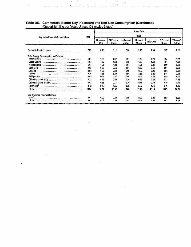
Table B5. Commercial Sector Key Indicators and End-Use Consumption (Continued)(Quadrillion Btu per Year, Unless Otherwise Noted)
Key Indicators and Consumption 1996
Projections
2005
ReferenceCase
24 PercentAbove
14 PercentAbove
9 PercentAbove
1990 Level3 Percent
Below7 Percent
Below
Electricity Related Losses " 7.52
Total Energy Consumption by End-UseSpace Heating 1.91Space Cooling 1.67WaterHeating 1.07Ventilation 0.55Cooking 0.28Lighting 3.76Refrigeration 0.45Office Equipment (PC) 0.22Office Equipment (non-PC) 0.63
OlherUses6 4.43
Total 14.98
Non-Marketed Renewable FuelsSolar7 0.01Total 0.01
8.23 8.11 7.78 7.46 7.36 7.37 7.27
1.881.701.080.570.303.880.470.250.78
5.5916.51
0.030.03
1.871.681.080.560.303.830.470.250.77
5.5616.37
0.030.03
1.811.621.040.540.293.680.460.240.74
5.38
15.80
0.030.03
1.761.561.010.520.283.530.460.230.715.22
15.29
O.O30.03
1.741.540.990.510.283.490.460.230.70
5.1615.10
0.030.03
1.741.540.990.510.28
' 3.480.460.230.70
5.16
15.09
0.030.03
1.721.520.980.500.283.440.460.230.70
5.10
14.93
0.030.03
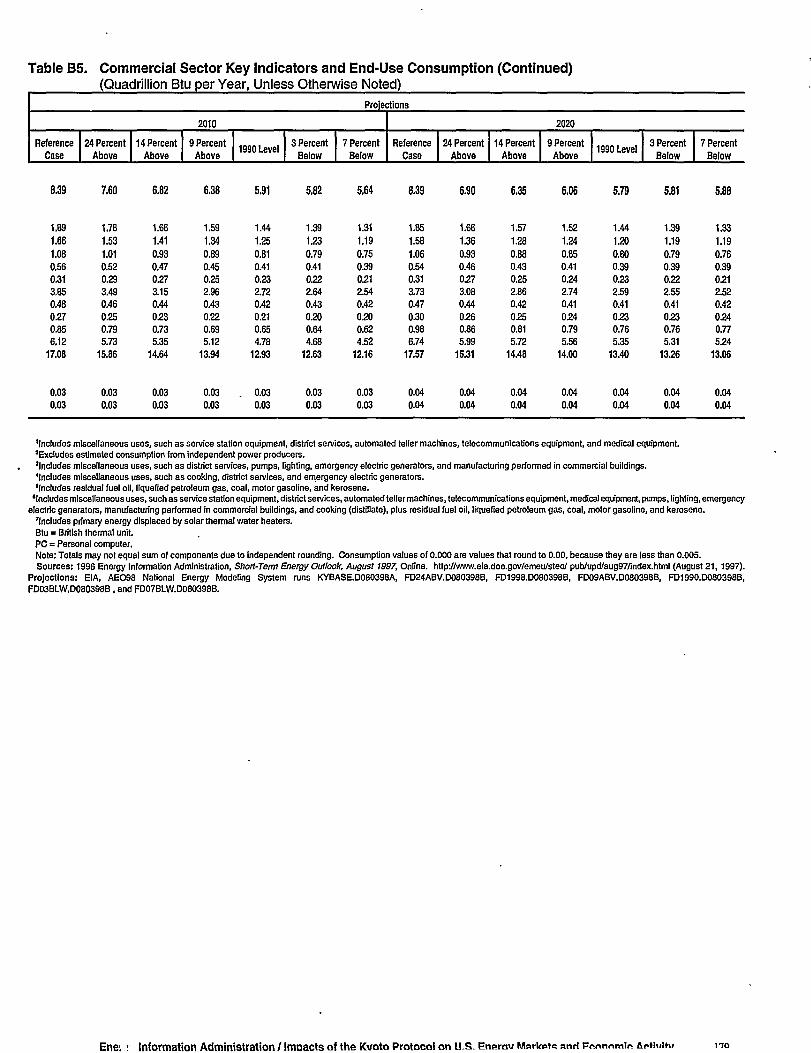
Table B5. Commercial Sector Key Indicators and End-Use Consumption (Continued)(Quadrillion Btu per Year, Unless Otherwise Noted)
Projections
2010
Reference
Case
24 Percent
Above
14 Percent
Above
9 Percent
Above1990 Level
3 Percent
Below
7 Percent
Below
2020
Reference
Case
24 Percent
Above
14 Percent
Above
9 Percent
Above1990 Level
3 Percent
Below
7 Percent
Below
8,39 7.60 6.82 6.38 5.91 5.82 5.64 8.39 6.90 6.35 6.06 5.79 5.81 5.88
1,89
1.661.080.56
0.31
3.85
0.48
0.27
0.85
6.12
17.08
0.03
0.03
1,78
1.53
1.01
0.52
0.29
3.49
0.46
0.25
0.79
5.73
15.86
0.03
0.03
1.66
1.410.93
0.47
0.27
3.15
0.44
0.23
0.73
5.35
14.64
0.03
0.03
1.59
1.34
0.89
0.45
0.25
2.96
0.43
0.22
0.69
5.12
13.94
0.03
0.03
1.44
1.25
0.81
0.41
0.23
2.72
0.42
0.21
0.65
4.78
12.93
. 0.03
0.03
1.39
1.23
0.79
0.41
0.22
2.64
0.43
0.20
0.64
4.68
12.63
0.03
0.03
1.31
1.19
0.75
0.39
0.21
2.54
0.42
0.20
0.62
4.52
12.16
0.03
0.03
1.85
1.58
1.06
0.54
0.31
3.73
0.47
0.30
0.98
6.74
17.57
0.04
0.04
1.66
1.36
0.93
0.46
0.27
3.08
0.44
0.26
0.86
5.99
15.31
0.04
0.04
1.57
1.28
0.88
0.43
0.25
2.86
0.42
0.25
0.81
5.72
14.48
0.04
0.04
1.52
1.24
0.85
0.41
0.24
2.74
0.41
0240.79
5.56
14.00
0.04
0.04
1.44
1.20
0.80
0.39
0.23
2.59
0.41
0230.76
5.35
13.40
0.04
0.04
1.39
1.19
0.79
0.39
0.22
2.55
0.41
0.23
0.76
5.31
1326
0.04
0.04
1.33
1.19
0.76
0.39
0.21
2.52
0.42
0.24
0.77
5.24
13.06
0.04
0.04
'Includes miscellaneous uses, such as service station equipment, district seivices, automated teller machines, telecommunications equipment, and medical equipment.'Excludes estimated consumption from independent power producers.'Includes miscellaneous uses, such as district seivices, pumps, lighting, emergency electric generators, and manufacturing performed in commercial buildings.'Includes miscellaneous uses, such as cooking, district services, and emergency electric generators.'Includes residual fuel oil, liquefied petroleum gas, coal, motor gasoline, and kerosene.
'Includes miscellaneous uses, such as service station equipment, district services, automated teller machines, telecommunications equipment, medical equipment, pumps, lighting, emergencyelectric generators, manufacturing performed in commercial buildings, and cooking (distillate), plus residual fuel oil, liquefied petroleum gas, coal, motor gasoline, and kerosene.
'Includes primary energy displaced by solar thermal v/ater heaters.Btu = British thermal unit.PC = Personal computer.Note: Totals may not equal sum of components due to independent rounding. Consumption values of 0.000 are values that round to 0.00, because they are less than 0.005.Sources: 1996 Energy Information Administration, Short-Term Energy Outlook, August 1997, Online, http://www.eia.doe.gov/emeu/steo/ pub/upd/aug97/index.html (August 21,1997).
Projections: EIA, AEO98 National Energy Modeling System runs KYBASE.D080398A, FD24ABV.D080398B, FD1998.D0S0398B, FD09ABV.D080398B, FD1990.D080398B,FD03BLW.D080398B, and FD07BLW.D080398B.
Enei < Information Administration / Imnacts of the Kvoto Protocol on U.S. Enerm/ Markets anri Pcnn &rti«iti»
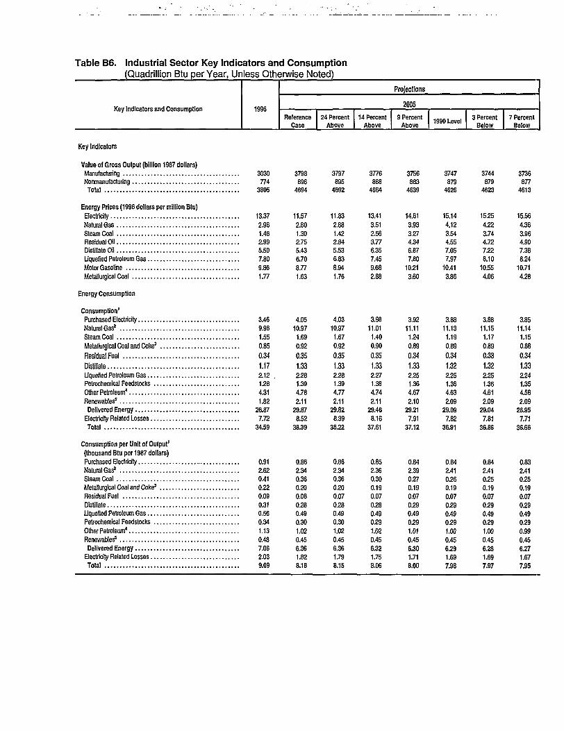
Table B6. Industrial Sector Key Indicators and Consumption(Quadrillion Btu per Year, Unless Otherwise Noted)
Key Indicators and Consumption 1996
Projections
2005
ReferenceCase
24 PercentAbove
14 PercentAbove
9 PercentAbove
1990 Level3 Percent
Below7 Percent
Below
Key Indicators
Value of Gross Output (billion 1987 dollars)
Manufacturing 3030
Nonmanufacturing 774
Total 3805
Energy Prices (1996 dollars per million Btu)
Electricity 13.37
Natural Gas 2.96
SteamCoal 1.46Residual Oil 2.99
Distillate Oil 5.50
Liquefied Petroleum Gas 7.80
MotorGasoline 9.86
Metallurgical Coal 1.77
Energy Consumption
Consumption1
Purchased Electricity 3.46
NaturalGas8 9.96
SteamCoal 1.55Metallurgical Coal and Coke3 0.85
Residual Fuel 0.34
Distillate 1.17
Liquefied Petroleum Gas 2.12
Petrochemical Feedstocks 1.28
Other Petroleum4 4.31
Renewables5 1.82
Delivered Energy 26.87Electricity Related Losses 7.72
Total 34.59
Consumption per Unit of Output'
(thousand Btu per 1987 dollars)
Purchased Electricity 0.91
NaturalGas* 2.62
Steam Coal 0.41
Metallurgical Coal and Coke3 0.22
ResidualFuel 0.09
Distillate 0.31
Liquefied Petroleum Gas 0.56
Petrochemical Feedstocks 0.34
Other Petroleum4 1.13
Renewables5 0.48
Delivered Energy 7.06
Electricity Related Losses 2.03
Total 9.09
3798896
4694
11.57
2.80
1.30
2.75
5.43
6.70
8.77
1.63
3797895
4692
11.83
2.88
1.42
2.84
5.53
6.83
8.94
1.76
3776888
4664
13.41
3.51
2.56
3.77
6.35
7.45
9.68
2.88
3756883
4639
14.61
3.93
3.27
4.34
6.87
7.80
10.21
3.60
3747
8794626
15.14
4.12
3.54
4.55
7.05
7.97
10.41
3.86
3744
8794623
15.25
4.22
3.74
4.72
7.22
8.10
10.55
4.06
3736877
4613
15.56
4.36
3.96
4.90
7.38
8.24
10.71
4.28
4.05
10.97
1.69
0.92
0.35
1.332.281.39
4.78
2.11
29.87
8.52
38.39
0.86
2.34
0.36
0.20
0.08
0.28
0.49
0.30
1.02
0.45
6.36
1.82
8.18
4.03
10.97
1.67
0.92
0.35
1.332.28
1.39
4.772.11
29.82
8.39
38.22
0.86
2.34
0.36
0.20
0.07
0.28
0.49
0.30
1.02
0.45
6.36
1.79
8.15
3.98
11.01
1.40
0.90
0.35
1.332.27
1.38
4.74
2.11
29.46
8.16
37.61
0.85
2.36
0.30
0.19
0.07
0.28
0.490.29
1.02
0.45
6.32
1.75
8.06
3.92
11.11
1.24
0.89
0.34
1.332.25
1.36
4.67
2.10
29.21
7.91
37.12
0.84
2.39
0.27
0.19
0.07
0.29
0.49
0.29
1.010.45
6.30
1.71
8.00
3.88
11.13
1.19
0.89
0.341.322.25
1.36
4.63
2.09
29.09
7.82
36.91
0.84
2.41
0.26
0.19
0.07
0.29
0.49
0.29
1.00
0.45
6.29
1.69
7.98
3.88
11.15
1.17
0.89
0.331.322.25
1.36
4.61
2.09
29.04
7.81
36.86
0.842.41
0.25
0.19
0.07
0.29
0.49
0.29
1.000.45
6.28
1.69
7.97
3.85
11.14
1.15
0.88
0.341.332.24
1.35
4.58
2.09
28.95
7.71
36.66
0.83
2.41
0.25
0.19
0.07
0.29
0.49
0.29
0.99
0.45
6.27
1.67
7.95
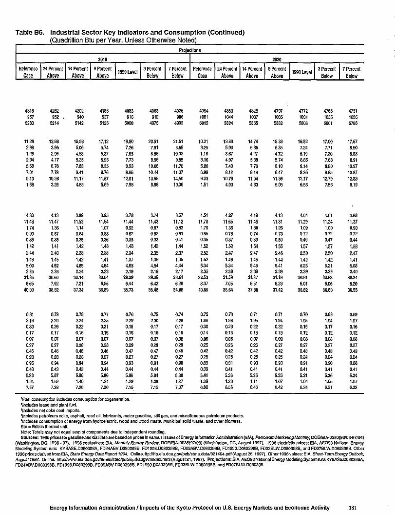
Table B6. Industrial Sector Key Indicators and Consumption (Continued)(Quadrillion Btu per Year, Unless Otherwise Noted)
Projections
2010
Reference
Case24 Percent
Above14 Percent
Above9 Percent
Above1990 Level
3 Percent
Below7 Percent
Below
2020
Reference
Case24 Percent
Above14 Percent
Above9 Percent
Above1990 Level
3 PercentBelow
7 PercentBelow
4316
9675283
11.28
2.98
1.26
2.94
5.68
7.01
9.13
1.58
4262
952 .
5214
13.86
3.96
2.96
4.17
6.76
7.79
10.26
3.28
4202
9405142
15.96
5.06
4.53
5.35
7.83
8.41
11.17
4.85
4188
9375126
17.12
5.74
5.37
5.96
8.35
8.76
11.57
5.69
4083
9165000
19.50
7.26
7.65
7.73
9.93
9.85
12.91
7.98
4063
9124975
20.51
7.81
8.65
8.56
10.66
10.44
13.55
8.98
4026
9064932
21.51
8.65
10.03
9.65
11.70
11.37
14.50
10.36
4954
1061
6015
10.31
3.25
1.18
3.16
5.86
6.99
9.33
1.51
4850
1044
5894
13.83
5.06
3.67
4.97
7.40
8.12
10.78
4.00
4828
1037
5865
14.74
5.86
4.27
5.39
7.76
8.18
11.04
4.60
4797
1035
5832
15.38
6.35
4.72
5.74
8.10
8.47
11.36
5.05
4772
1031
5803
16.52
7.24
6.19
6.85
9.14
9.36*
12.17
6.55
4766
1035
5801
17.00
7.71
7.20
7.63
9.80
9.95
12.79
7.56
4751
1036
5786
17.67
8.50
8.83
8.91
10.97
10.87
13.83
9.19
4,30
11,43
1.74
0.90
0,35
1.422.441.48
5.03
2.25
31.35
8,65
40.00
0,81
2,16
0,33
0.17
0,07
0,27
0.46
0.28
0.95
0.43
5.93
1.64
7.57
4.13
11.47
1.36
0.87
0.35
1.412.401.45
4.92
2.25
30.60
7.92
38.52
0.79
2.20
0.26
0.17
0.07
0.27
0.46
0.28
0.94
0.43
5.87
1.52
7.39
3.99
11.52
1.14
0.84
0.35
1.42
2.38
1.42
4.85
2.24
30.14
7.21
37.34
0.78
2.24
0.22
0.16
0.07
0.28
0.46
0.28
0.94
0.43
5.86
1.40
7.26
3.95
11.54
1.07
0.83
0.36
1.43
2.38
1.41
4.84
2.23
30.04
6.85
36.89
0.77
2.25
0.21
0.16
0.07
0.28
0.46
0.27
0.94
0.44
5.86
1.34
7.20
3.78
11.44
0.92
0.82
0.35
1.43
2.34
1.37
4.65
2.19
29.29
6.44
35.73
0.76
2.29
0.18
0.16
0.07
0.29
0.47
0.27
0.93
0.44
5.86
1.29
7.15
3.74
11.43
0.87
0.82
0.33
1.43
2.35
1.36
4.54
2.18
29.05
6.43
35.48
0.75
2.30
0.17
0.16
0.07
0.29
0.47
0.27
0.91
0.44
5.84
1.29
7.13
3.67
11.12
0.83
0.81
0.41
1.44
2.37
1.35
4.44
2.17
28.61
6.28
34.88
0.74
2.26
0.17
0.16
0.08
0.29
0.48
0.27
0.90
0.44
5.80
1.27
7.07"
4.51
11.78
1.79
0.85
0.35
1.52
2.52
1.52
5.34
2.35
32.53 .
8.37
40.89
0.75
1.96
0.30
0.14
0.06
0.25
0.42
0.25
0.89
0.39
5.41
1.39
6.80
4.27
11.65
1.36
0.76
0.37
1.52
2.47
1.46
5.34
2.39
31.59
7.05
38.64
0.73
1.98
0.23
0.13
0.06
0.26
0.42
0.25
0.91
0.41
5.36
1.20
6.56
4.19
11.45
1.30
0.74
0.39
1.54
2.47
1.45
5.45
2.39
31.37
6.51
37.88
0.71
1.95
0.22
0.13
0.07
0.26
0.42
0.25
0.93
0.41
5.35
1.11
6.46
4.13
11.31
1.26
0.73
0.50
1.55
2.46
1.44
5.41
2.39
31.19
6.23
37.42
0.71
1.94
0.22
0.13
0.09
0.27
0.42
0.25
0.93
0.41
5.35
1.07
6.42
4.04
11.29
1.09
0.72
0.49
1.57
2.50
1.42
5582.39
30.81
6.01
36.82
0.70
1.95
0.19
0.12
0.08
0.27
0.43
0.24
0.91
0.41
5.31
1.04
6.34
4.01
11.24
1.00
0.72
0.47
1.57
2.50
1.425.21
2.39
30.53
6.06
36.60
0.69
1.94
0.17
0.12
0.08
0.27
0.43
0.24
0.90
0.41
5.26
1.05
6.31
3.98
11.37
0.900.72
0.44
1.58
2.471.41
5.08
2.40
30.34
6.20
36.55
0.69
1.97
0.16
0.12
0.08
0.27
0.43
0.24
0.88
0.41
5541.07
6.32
'Fuel consumption Includes consumption for cogeneration.
'Includes lease and plant fuel.'Includes net coke coal imports.'Includes petroleum coke, asphalt, road oil, lubricants, motor gasoline, still gas, and miscellaneous petroleum products.'Includes consumption of energy from hydroelectric, wood and wood waste, municipal solid waste, and other biomass.Btu = British thermal unit.Note: Totals may not equal sum of components due to independent rounding.Sources: 1996 prices for gasoline and distillate are based on prices in various issues of Energy Information Administration (El A), Petroleum Marketing Monthly, DOE/El A-0380(96/03-97/04)
(Washington, DC, 1996 - 97). 1996 coal prices: EIA, Monthly Energy Review, DOE/EIA-0035(97/08) (Washington, DC, August 1997). 1996 electricity prices: EIA, AEO98 National EnergyModeling System runs KYBASE.D080398A, FD24ABV.D080398B, FD1998.D080398B, FD09ABV.D080398B, FD1990.D080398B, FD03BLW.D080398B, and FD07BLW.D080398B. Other1996 prices derived from El A, State Energy Data Report 1994. Online, ftp://ftp.eia.doe.gov/pub/state.data/021494.pdf (August 26,1997). Other 1996 values: El A, Short-Term Energy Outlook,August 1997. Online. http://www.eia.doe.gov/emeu/steo/pub/upd/aug97Andex.html (August 21,1997). Projections: EIA, AEO98 National Energy Modeling System runs KYBASE.D080398A,FD24ABV.D080398B, FD1998.D080398B, FD09ABV.D080398B, FD1990.D080398B, FD03BLW.D080398B, and FD07BLW.D080398.
Energy Information Administration / Impacts of the Kyoto Protocol on U.S. Energy Markets and Economic Activity 181
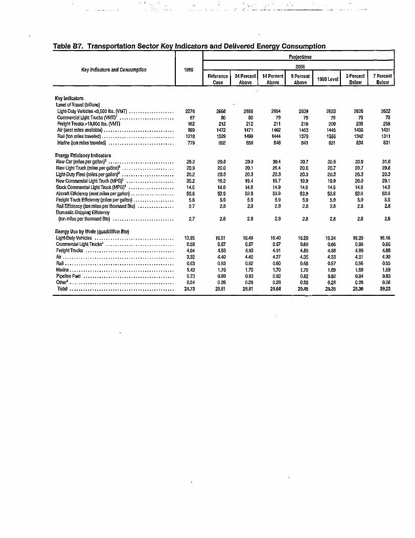
Table B7. Transportation Sector Key Indicators and Delivered Energy Consumption
Key Indicators and Consumption 1996
Projections
2005
ReferenceCase
24 PercentAbove
14 PercentAbove
9 PercentAbove
1990 Level 3 PercentBelow
7 PercentBelow
Key IndicatorsLevel of Travel (billions)Light-Duty Vehicles <8,500 lbs. (VMT) 2276Commercial Light Trucks (VMT)1 67Freight Trucks >10,000 lbs. (VMT) 162Air (seat miles available) 999Rail (ton miles traveled) 1218Marine (ton miles traveled) 779
Energy Efficiency IndicatorsNew Car (miles per gallon)2 28.2New Light Truck (miles per gallon)2 20.9Light-Duty Fleet (miles per gallon)3 20.2New Commercial Light Truck (MPG)1 20.2Stock Commercial Light Truck (MPG)1 14.5Aircraft Efficiency (seat miles per gallon) 50.6Freight Truck Efficiency (miles per gallon) 5.6Rail Efficiency (ton miles per thousand Btu) 2.7Domestic Shipping Efficiency(ton milesperthousand Btu) 2.7
Energy Use by Mode (quadrillion Btu)Light-Duty Vehicles 13.95Commercial Light Trucks1 0.58Freight Trucks 4.04Air 3.32Rail 0.53Marine 1.43Pipeline Fuel 0.73Other1 0.24Total 24.73
266880
21214721529862
29.820.020.319.314.853.95.92.8
266580
21214711499859
29.920.120.319.414.853.95.92.8
265479
21114621444848
30.420.420.319.714.953.95.92.8
263979
21014531379841
30.720.620.319.914.953.95.92.8
263379
20914451356831
30.820.720.319.914.953.85.92.8
262679
20914381342834
30.920.720.320.014.953.85.92.8
262278
20814311311831
31.020.820.320.114.953.85.92.8
2.8 2.8 2.8 2.8 2.8 2.8 2.8
16.510.674.934.400.631.700.800.28
29.81
16.490.674.934.400.621.700.830.28
29.81
16.400.674.914.370.601.700.820.28
29.64
16.290.664.894.350.581.700.820.28
29.45
16.240.664.884.330.571.690.820.28
29.35
16.200.664.884.310.561.690.840.28
29.30
16.160.664.884.300.551.690.830.28
29.22
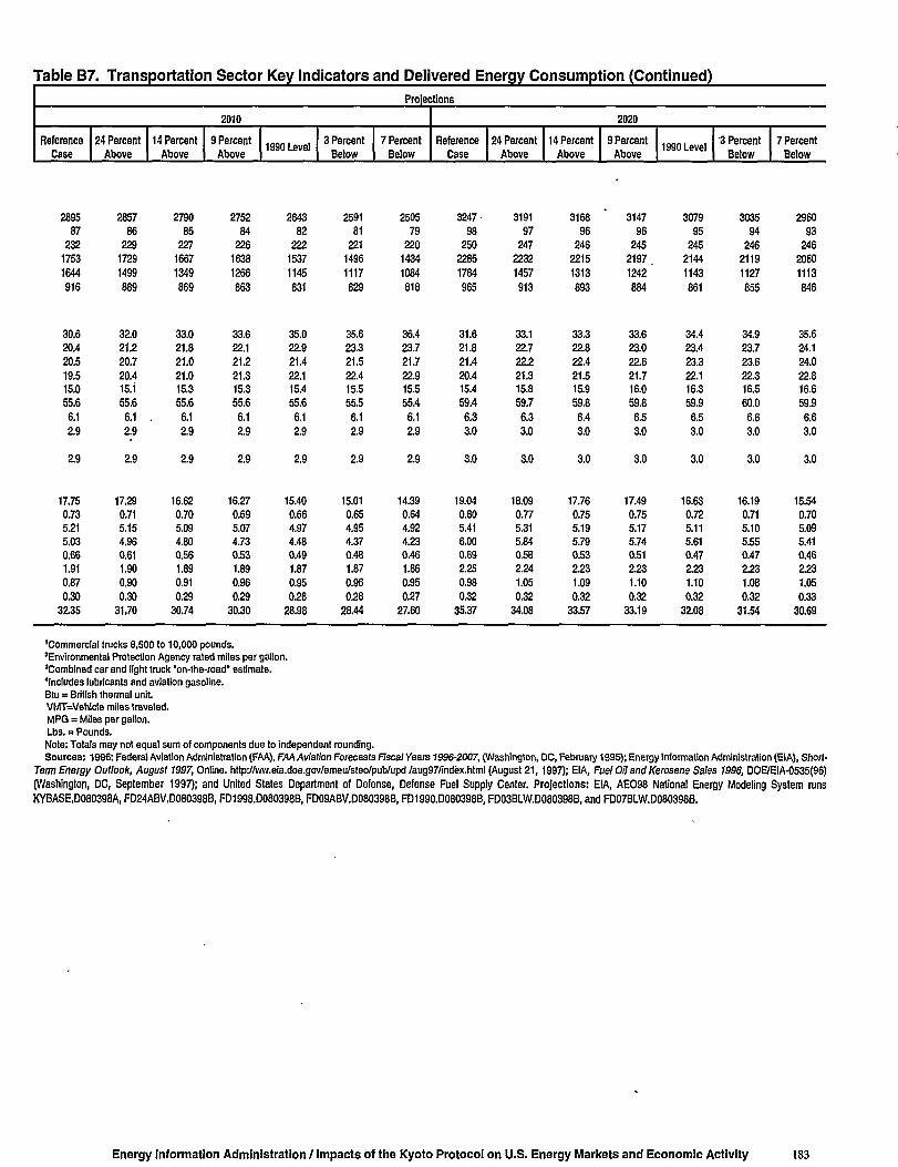
Table B7. Transportation Sector Key Indicators and Delivered Energy Consumption (Continued)Projections
2010 2020
ReferenceCase
24 PercentAbove
14 PercentAbove
9 PercentAbove
1990 Level 3 PercentBelow
7 PercentBelow
ReferenceCase
24 PercentAbove
14 PercentAbove
9 PercentAbove 1990 Level 3 Percent
Below7 Percent
Below
28958723217531644916
30,620.420.519,515.055,66.12.9
28578622917291499889
32.021.220.720.415.155.66.1 .2.9
27908522716671349869
33.021.821.021.015.355.66.12.9
27528422616381266863
33.622.121.221.315.355.66.12.9
26438222215371145831
35.022.921.422.115.455.66.12.9
25918122114961117829
35.623.321.522.415.555.56.12.9
25057922014341084818
36.423.721.722.915.555.46.12.9
3247-9825022851784965
31.621.821.420.415.459.46.33.0
319197247
22321457913
33.122.722.221.315.859.76.33.0
316896246
22151313893
33.322.822.421.515.959.86.43.0
3147962452197.1242884
33.623.022.621.716.059.86.53.0
307995245
21441143861
34.423.423.322.116.359.96.53.0
30359424621191127855
34.923.723.622.316.560.06.63.0
29609324620601113846
35.624.124.022.816.659.96.63.0
2.9 2.9 2.9 2.9 2.9 2.9 2.9 3.0 3.0 3.0 3.0 3.0 3.0 3.0
17.750.735.215.030.661.910,870.3032.35
17.290.715,154.960.611.900.900.3031.70
16.620.705.094.800,561.890.910.29
30.74
16.270.695.074.730.531.890.960.2930.30
15.400.664.974.480.491.870.950.2828.98
15.010.654.954.370.481.870.960.28
28.44
14.390.644.924.230.461.860.950.27
27.60
19.040.805.416.000.692.250.980.32
35.37
18.090.775.315.840.582.241.050.3234.03
17.760.755.195.790.532.231.090.32
33.57
17.490.755.175.740.512.231.100.32
33.19
16.630.725.115.610.472.231.100.3232.08
16.190.715.105.550.472.231.080.3231.54
15.540.705.095.410.462.231.050.3330.69
'Commercial trucks 8,500 to 10,000 pounds.'Environmental Protection Agency rated miles per gallon.'Combined car and light truck 'on-the-road' estimate.'Includes lubricants and aviation gasoline.Btu = British thermal unit.VMT=Veh!cle miles traveled.MPG = Miles per gallon.Lbs. = Pounds.Note: Totals may not equal sum of components due to independent rounding.Sources: 1996: Federal Aviation Administration (FAA), FAA Aviation Forecasls Fiscal years 1996-2007, (Washington, DC, February 1995); Energy Information Administration (EIA), Short-
Tern; Energy Outlook, August 1997, Online, http://ww.eia.doe.gov/emeu/steo/pub/upd /aug97/index.html (August 21,1997); EIA, Fuel Oil and Kerosene Sales 1996, DOE/EIA-0535(96)(Washington, DC, September 1997); and United States Department of Defense, Defense Fuel Supply Center. Projections: EIA, AEO98 National Energy Modeling System runsKYBASE,D080398A, FD24ABV.D080398B, FD1998.D080398B, FD09ABV.D080398B, FD1990.D080398B, FD03BLW.D080398B, and FD07BLW.D080398B.
Energy Information Administration / Impacts of the Kyoto Protocol on U.S. Energy Markets and Economic Activity 183

Table B8. Electricity Supply, Disposition, and Prices
(Billion Kilowatthours, Unless Otherwise Noted)
Supply, Disposition, and Prices 1996
Projections
2005
ReferenceCase
24 PercentAbove
14 PercentAbove
9 PercentAbove
1990 Level3 PercentBelow
7 PercentBelow
Generation by Fuel TypeElectric Generators1
Coal 1758Petroleum 80Natural Gas 288Nuclear Power 675Pumped Storage -2Renewable Sources2 392Total 3191
Non-Utility Generation for Own Use 6
Cogenerators3
Coal 51Petroleum . . : 6Natural Gas 196OtherGaseous Fuels4 7Renewable Sources2 42Other5 3Total 305
Salesto Utilities 156Generation for Own Use 149
Net Imports6 38
Electricity Sales by SectorResidential 1079Commercial 988Industrial 1014Transportation 17Total 3098
End-Use Prices (1996 cents per kilowatthour)7
Residential 8.3Commercial 7.5Industrial 4.6Transportation 5.2
All Sectors Average . . . 6 . 8
2019
42612651-33693690
6
516
2147473
329161168
67
12711147118824
3630
7.46.63.94.66.0
1949
41671683-33793720
6
516
2147473
329161168
21
12651143118324
3615
7.56.74.04.66.1
1820
37714683-33853637
6
516
2187473
332161171
21
12351112116724
3538
8.47.64.64.76.9
1681
36777683-3
3853559
6
506
2227463
335162174
21
12101084114924
3467
9.18.35.04.87.4
1597
34807698-3
3923525
6
506
2247463
337162175
21
12011071113824
3435
9.48.65.24.87.7
1556
32841698-33963519
6
506
2237463
337162175
21
11991071113624
3430
9.58.75.24.87.8
1504
35863698-3
4013498
6
506
2247463
337162175
21
11931064112924
3410
9.68.85.34.87.9
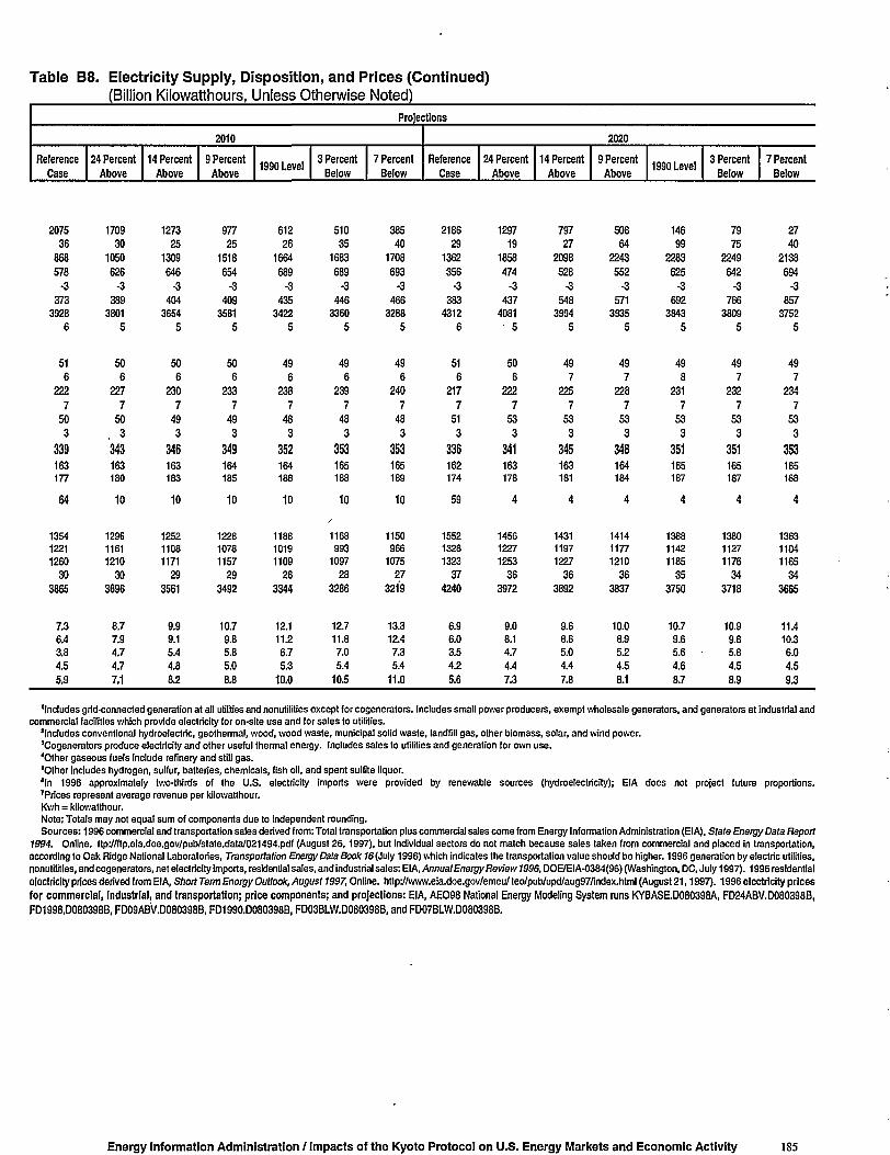
Table B8. Electricity Supply, Disposition, and Prices (Continued)(Billion Kilowatthours, Unless Otherwise Noted)
Projections
2010
ReferenceCase
207536868578-337339286
516
2227503339163177
24 PercentAbove
170930
1050626-338938015
506
2277503
'343163180
14 PercentAbove
127325
1309646-340436545
506
2307493346163183
9 PercentAbove
97725
1518654-340935815
506
2337493
349164185
1QQn t mrallasU Level
61226
1664689-343534225
496
2387483
352164188
3 PercentBelow
51035
1683689-3
44633605
496
2397483
353165188
7 PercentBelow
38540
1708693-3
46632885
496
2407483
353165189
2020
ReferenceCase
218629
1362356-338343126
516
2177513
336162174
24 PercentAbove
129719
1858474-343740815
506
2227533
341163178
14 PercentAbove
79727
2098528-354839945
497
2257533
345163181
9 PercentAbove
50864
2243552-3571
39355
497
2287533
348164184
loon t ouoiI99U Level
14699
2283625-369238435
498
2317533
351165187
3 PercentBelow
7975
2249642-376638095
497
2327533
351165187
7 PercentBelow
2740
2138694-385737525
497
2347533
353165188
64 10 10 10 10 10 10 59
13541221126030
3865
7.36.43.84,55,9
12961161121030
3696
8.77.94.74.77.1
12521108117129
3561
9.99.15.44.88.2
12281078115729
3492
10.79.85.85.08.8
11881019110928
3344
12.111.26.75.310.0
1168993109728
3286
12.711.87.05.4
10.5
1150966107527
3219
13.312.47.35.411.0
15521328132337
4240
6.96.03.54.25.6
14561227125336
3972
9.08.14.74.47.3
14311197122736
3892
9.68.65.04.47.8
14141177121036
3837
10.08.95.24.58.1
13881142118535
3750
10.79.65.6 •
4.68.7
13801127117634
3718
10.99.85.84.58.9
13631104116534
3665
11.410.36.04.59.3
'Includes grid-connected generation at all utilities and nonutilities except for cogenerators. Includes small power producers, exempt wholesale generators, and generators at industrial andcommercial facilities which provide electricity for on-site use and for sales to utilities.
'Includes conventional hydroelectric, geolhermal, wood, wood waste, municipal solid waste, landfill gas, other biomass, solar, and wind power.'Cogenerators produce electricity and other useful thermal energy. Includes sales to utilities and generation for own use.'Other gaseous fuels include refinery and still gas."Other includes hydrogen, sulfur, batteries, chemicals, fish oil, and spent sulfite liquor."In 1996 approximately two-thirds of the U.S. electricity imports were provided by renewable sources (hydroelectricity); EIA does not project future proportions.'Prices represent average revenue per kilowatthour.Kwh = kilowatthour.Note; Totals may not equal sum of components due to independent rounding.Sources: 1996 commercial and transportation sales derived from: Total transportation plus commercial sales come from Energy Information Administration (EIA), State Energy Data Report
1994. Online, ftp://ftp.ela.doe.gov/pub/state.data/021494.pdf (August 26,1997), but individual sectors do not match because sales taken from commercial and placed in transportation,according to Oak Ridge National Laboratories, Transportation Energy Data Book J6(July 1996) which indicates the transportation value should be higher. 1996 generation by electric utilities,nonutilities, and cogenerators, net electricity imports, residential sales, and industrial sales: EIA, Annual Energy Review 1996, DOE/EIA-0384(96) (Washington, DC, July 1997). 1996 residentialelectricity prices derived from EIA, Short Term Energy Outlook, August 1997, Online, http://www.eia.doe.gov/emeu/teo/pub/upd/aug97/index.html (August 21,1997). 1996 electricity pricesfor commercial, Industrial, and transportation; price components; and projections: EIA, AEO98 National Energy Modeling System runs KYBASE.D080398A, FD24ABV.D080398B,FD1998.D080398B, FD09ABV.D080398B, FD1990.D080398B, FD03BLW.D080398B, and FD07BLW.D080398B.
Energy Information Administration / Impacts of the Kyoto Protocol on U.S. Energy Markets and Economic Activity 185

Table B9. Electricity Generating Capability(Thousand Megawatts)
Net Summer Capability11996
Projections
2005
Reference
Case
24 Percent
Above
14 Percent
Above
9 Percent
Above1990 Level
3 Percent
Below
7 PercentBelow
Electric Generators2
Capability
CoalSteam 303.7Other Fossil Steam3 136.6Combined Cycle 15.2Combustion Turbine/Diesel 61.6Nuclear Power 100.8Pumped Storage 19.9Fuel Cells 0.0Renewable Sources4 87.8Total 725.5
Cumulative Planned Additions5
Coal Steam 2.1
Other Fossil Steam3 0.0
Combined Cycle 2.0
Combustion Turbine/Diesel 3.8
NudearPower 1.2
Pumped Storage 1.1
Fuel Cells 0.0Renewable Sources' 0.7Total 11.1
Cumulative Unplanned Additions5
CoalSteam 0.0
Other Fossil Steam3 0.0
Combined Cycle 0.0
Combustion Turbine/Diesel 5.7
Nuclear Power 0.0
Pumped Storage 0.0
Fuel Cells 0.0
Renewable Sources4 0.8
Total 6.6
Cumulative Total Additions 17.7
Cumulative Retirements6 15.2
305.3
128.2
50.7
123.9
89.6
19.9
0.091.1
808.8
2.90.12.75.21.21.10.03.1
16.3
3.10.0
34.2
68.4
0.00.00.01.4
107.1
123.4
40.1
302.1
126.0
61.6
115.6
94.1
19.9
0.091.3
810.5
2.90.12.75.21.21.10.03.1
16.3
0.00.0
45.1
59.6
0.00.00.01.6
106.2
122.5
37.5
302.1
125.6
66.0
105.7
94.1
19.9
0.092.5
805.9
2.90.12.75.21.21.10.03.1
16.3
0.00.0
49.5
49.7
0.00.00.02.9
102.1
118.4
38.0
302.1
125.4
74.7
99.0
94.1
19.9
0.093.1
808.2
2.90.12.75.21.21.10.03.1
16.3
0.00.0
58.2
43.3
0.00.00.03.4
104.9
121.2
38.5
302.0
125.4
72.6
99.2
96.1
19.9
0.094.8
810.0
2.90.12.75.21.21.10.03.1
16.3
0.00.0
56.1
43.3
0.00.00.05.1
104.5
120.8
36.4
301.9
126.1
70.8
99.3
96.1
19.9
0.095.7
809.8
2.90.12.75.21.21.10.03.1
16.3
0.00.0
54.3
43.7
0.00.00.06.0
104.1
120.4
36.1
301.9
124.4
78.5
96.2
96.1
19.9
0.097.0
814.0
2.90.12.75.21.21.10.03.1
16.3
0.00.0
62.0
40.4
0.00.00.07.3
109.7
126.0
37.5
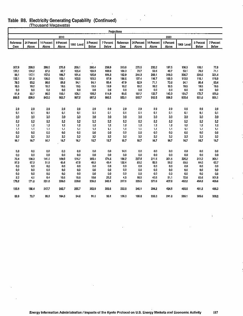
Table B9. Electricity Generating Capability (Continued)(Thousand Megawatts)
Projections
2010 2020
Reference
Case
24 Percent
Above
14 Percent
Above
9 PercentAbove
1990 Level3 Percent
Below
7 PercentBelow
Reference
Case
24 Percent
Above
14 PercentAbove
9 Percent
Above1990 Level
3 Percent
Below
7 PercentBelow
307.8
123.1
90,1
152.1
76,0
19,5
0,091.8
860.5
2,90.13,05,21.21.10,03.2
16.7
5,80,0
73.497.9
0,00,00,02.2
179.2
195.8
60.9
299.9
104,2
117.1121.883.219.2
0.093.7
839.2
2.90.13,05,21.21.10.03,2
16.7
0.00.0
100,3
67.3
0.00,00,04,1
171.8
188.4
73.7
288.5
87.0
157.6
106.0
86.6
19.2
0.098.0
843.0
2.90.13.05.21.21.10.03.2
16.7
0.00.0
141.151.5
0.00.00.08.4
201.0
217.7
99.2
275.8
92.7
186.7
100.1
88.8
19.5
0.0100.1
863.7
2.90.13.05,21.21.10.03,2
16.7
0.00.0
169.9
45.6
0.00.00.0
10.5
226.0
242.7
104.5
268.1
105.4
191.4
102.5
94.1
19.5
0.0106.1
887.2
2.90.13.05.21.21.10.03.2
16.7
0.00.0
174.7
47.8
0.00.00.0
16.5
239.0
255.7
94.0
266.4
109.8
185.9
103.5
94.1
19.5
0.0108.2
887.3
2.90.13.05.21.21.10.03.2
16.7
0.00.0
169.1
48.5
0.00.00.0
18.6
236.2
252.9
91.1
258.9
108.0
191.3
97.9
95.4
19.9
0.0114.9
886.2
2.90.13.05.21.21.10.03.2
16.7
0.00.0
174.5
43.4
0.00.00.0
25.2
243.1
259.8
99.1
313.6
109.3
182.9
186.6
47.9
19.2
0.093.6
953.1
2.90.13.05.21.21.10.03.2
16.7
14.10.0
166.2132.4
0.00.00.04.5
317.1
333.8
106.3
270.5
73.7
244.3
137.4
62.9
19.2
0.0107.7
915.7
2.90.13.05.21.21.10.03.2
16.7
0.00.0
227.883.2
0.00.00.0
18.5
329.5
346.1
155.0
232.2
53.6
288.1
116.7
71.119.2
0.0132.7
913.5
2.90.13.05.21.21.10.03.2
16.7
0.00.0
271.5
62.5
0.00.00.0
43.5
377.6
3945
205.3
197.5
49.7
318.0
109.3
73.8
19.50.0
140.3
9085
2.90.1
3.05.2151.10.03.2
16.7
0.00.0
301.555.2
0.00.00.0
51.1
407.8
424.5
241.8
136.3
53.1
336.7
113.9
84.1
19.5
0.0161.7
905.4
2.90.13.05.2151.10.03.2
16.7
0.00.0
320.2
59.5
0.00.00.0
72.6
4525
468.9
288.1
100.1
70.2
334.0
118.1
86.4
19.5
0.0172.7
901.0
2.90.13.05.2151.10.03.2
16.7
0.00.0
317.2
64.0
0.00.00.0
83.6
464.8
481.5
305.6
77.8
71.1
321.4
116.9
93.4
'19.5
0.0191.0
891.1
2.90.13.05.2151.10.03.2
16.7
0.00.0
305.1
62.7
0.00.00.0
101.8
469.6
486.3
3205
Energy Information Administration / Impacts of the Kyoto Protocol on U.S. Energy Markets and Economic Activity 187

Table B9. Electricity Generating Capability (Continued)(Thousand Megawatts)
Net Summer Capability1 1996
Projections
2005
ReferenceCase
24 PercentAbove
14 PercentAbove
9 PercentAbove
1990 Level 3 PercentBelow
7 PercentBelow
Cogenerators7
CapabilityCoalPetroleumNatural GasOther Gaseous Fuels .Renewable Sources4..OtherTotal
Cumulative Additions5
9.21.2
31.41.25.90.0
48.8
9.91.3
34.91.16.90.0
54.2
9.91.3
35.01.16.90.0
54.2
9.91.3
35.41.16.80.0
54.6
9.9 •1.3
36.01.16.80.0
55.0
9.81.3
36.31.16.80.0
55.3
9.81.3
36.21.16.80.0
55.2
9.81.3
36.21.16.80.0
55.3
18.2 23.6 23.6 23.9 24.4 24.7 24.6 24.6

Table B9. Electricity Generating Capability (Continued)(Thousand Megawatts)
Projections
2010
ReferenceCase
24 PercentAbove
14 PercentAbove
9 PercentAbove
1990 Level3 Percent
Below7 Percent
Below
2020
ReferenceCase
24 PercentAbove
14 PercentAbove
9 PercentAbove
1990 Level3 Percent
Below7 Percent
Below
10,01,3
36,0
1.17.10.0
55.6
24.9
10.01.3
36.61.17.10.0
56.1
25.5
9.91.3
37.11.17.10.0
56.6
25.9
9.91.3
37.51.17.10.0
56.9
26.3
9.81.3
38.21.1
'6.90.0
57.4
26.7
9.81.3
38.31.16.90.0
57.5
26.8
9.81.3
38.41.16.90.0
57.5
26.9
10.01.3
35.41.17.30.0
555
24.6
10.01.3
36.11.17.40.0
56.0
25.4
10.01.3
36.61.17.40.0
56.5
25.8
10.01.3
37.01.17.40.0
56.9
252
9.91.3
37.61.17.40.0
57.4
26.7
9.91.3
37.71.17.40.0
57.4
26.8
9.91.3
37.81.17.40.0
57.6
27.0
'Net summer capability is the steady hourly output that generating equipment is expected to supply to system load (exclusive of auxiliary power), as demonstrated by tests during summerpeak demand.'Includes grid-connected utilities and nonutilities except (or cogenerators. Includes small power producers, exempt wholesale generators, and generators at industrial and commercial facilities
which produce electricity for on-site use and sales to utilities.'Includes oil-, gas-, and dual-fired capability.'Includes conventional hydroelectric, geothermal, wood, wood waste, municipal solid v/aste, landfill gas, other biomass, solar and wind power.'Cumulative additions after December 31,1995.'Cumulative total retirements from 1990.7Nameplate capacity Is reported for nonutilities on Form EIA-867, "Annual Power Producer Report." Nameplate capacity is designated by the manufacturer. The nameplate capacity has
been converted to the net summer capability based on historic relationships.Notes: Totals may not equal sum of components due to independent rounding. Net summer capability has been estimated for nonutility generators for AEO9S. Net summer capacity is used
to be consistent with electric utility capacity estimates. Data for electric utility capacity are the most recent data available as of August 25,1997. Therefore, capacity estimates may differ fromother Energy Information Administration sources.
Sources: 1996 net summer capability at electric utilities and planned additions: Energy Information Administration (EIA), Form EIA-860, "Annual Electric Generator Report." Net summercapability for nonutilities and cogeneration in 1996 and planned additions estimated based on EIA, Form EIA-867, "Annual Nonutility Power Producer Report." Projections: EIA, AEO98National Energy Modeling System runs KYBASE.D080398A, FD24ABV.D080398B, FD1998.D080398B, FD09ABV.D080398B, FD1990.D080398B, FD03BLW.D080398B, andFD07BLW.D080398B.
Energy Information Administration / Impacts of the Kyoto Protocol on U.S. Energy Markets and Economic Activity 189

Table B10. Electricity Trade(Billion Kilowatthours, Unless Otherwise Noted)
Electricity Trade 1996
Projections
2005
ReferenceCase
24 PercentAbove
14 PercentAbove
9 PerceniAbove
1990 Level3 Percent
Below7 Percent
Below
Interregional Electricity Trade
Gross Domestic Rrm Power Sales 173.4Gross Domestic Economy Sales 54.7
Gross Domestic Trade 228.1
Gross Domestic Rrm Power Sales(million 1996 dollars) 8050.2
Gross Domestic Economy Sales(million 1996 dollars) 1283.9Gross Domestic Sales(million 1996 dollars) 9334.1
International Electricity Trade
Rrm Power Imports From Canada and Mexico1 26.1Economy Imports From Canada and Mexico1 20.7Gross Imports From Canada and Mexico1 46.8
Rrm Power Exports To Canada and Mexico 2.8Economy Exports To Canada and Mexico 6.4Gross Exports To Canada and Mexico 9.3
139.266.3
205.5
6462.9
1551.5
8014.3
51.435.887.2
13.4
7.0
20.3
139.277.5
216.7
6462.9
1801.0
8263.9
5.635.841.5
13.47.0
20.3
139.258.3
197.5
6462.9
1919.6
8382.5
5.635.941.5
13.47.0
20.3
139.249.8
189.0
6462.9
1914.1
8377.0
5.635.941.5
13.47.0
20.3
139.246.7
185.9
6462.9
1889.6
8352.5
5.635.941.5
13.47.0
20.3
139.250.5
189.7
6462.9
2125.6
8588.4
5.635.841.4
13.47.0
20.3
139.251.8
191.0
6462.9
2204.0
8666.9
5.635.841.5
13.47.0
20.3

Table B10. Electricity Trade (Continued)(Billion Kilowatthours, Unless Otherwise Noted)
Projections
2010
ReferenceCase
24 PercentAbove
14 PercentAbove
9 PercentAbove
1990 Level3 Percent
Below7 Percent
Below
2020
ReferenceCase
24 PercentAbove
14 PercentAbove
9 PercentAbove
1990 Level3 Percent
Below7 Percent
Below
139.266,2
205.4
6462.9
1567.0
8029.9'
51.433.484.8
13,4
7-721,0
139.254.8
194.0
6462.9
1918.0
8380.9
5.625,531.1
13,4
7,721.0
139.239.6
178.8
6462.9
1884.0
8346.8
5.625.531.1
13.4
7.721.0
139.227.2
166.4
6462.9
1467.6
7930.5
5.625.531.1
13.4
7.721.0
139.229.7
168.9
6462.9
2017.4
8480.3
5.625.130.7
13.4
7.721.0
139.227.7
167.0
6462.9
2071.5
8534.4
5.625.230.8
13.4
• 7.7
21.0
139239.6
178.8
6462.9
3356.4
9819.3
5.625.230.8
13.4
7.721.0
139281.5
220.7
6462.9
1831.8
8294.7
50.330.180.4
13.4
7.721.0
139263.3
202.5
6462.9
2478.3
89412
5.619.6252
13.4
7.721.0
139252.0
191.3
6462.9
2210.6
8673.4
5.619.6252
13.4
7.721.0
1392442
183.4
6462.9
2013.1
8475.9
5.619.6252
13.4
7.721.0
139251.4
190.6
6462.9
2640.1
9103.0
5.619.6252
13.4
7.721.0
139267.0
2062
6462.9
3602.1
10065.0
5.619.6252
13.4
7.7
21.0
139264.5
203.7
6462.9
3901.1
10364.0
5.619.6252
13.4
7.721.0
'Historically electric Imports were primarily from renewable resources, principally hydroelectric.Note: Totals may not equal sum of components due to independent rounding. Firm Power Sales are capacity sales, meaning the delivery of the power is scheduled as part of the normal
operating conditions of the affected electric systems. Economy Sales are subject to curtailment or cessation of delivery by the supplier in accordance with prior agreements or under specifiedconditions.
Sources: 1996 interregional electricity trade data: Energy Information Administration (EIA), Bulk Power Data System. 1996 international electricity trade data: DOE Form FE-718R, 'AnnualReport of International Electrical Export/Import Data." Firm/economy share: National Energy Board, Annual Report 1993. Planned interregional and international firm power sales: DOE FormIE-411, 'Coordinated Bulk Power Supply Program Report," April 1995. Projections: EIA, AEO98 National Energy Modeling System runs KYBASE.D080398A, FD24ABV.D080398B.FD1998.D080398B, FD09ABV.D080398B, FD1990.D080398B, FD03BLW.D080398B, and FD07BLW.D080398B.
Energy Information Administration / Impacts of the Kyoto Protocol on U.S. Energy Markets and Economic Activity 191

Table B11. Petroleum Supply and Disposition Balance(Million Barrels per Day, Unless Otherwise Noted)
Supply and Disposition 1996
Projections
2005
Reference
Case
24 Percent
Above
14 Percent
Above
9 Percent
Above1990 Level
3 Percent
Below
7 Percent
Below
Crude OilDomesticCrude Production1 6.48
Alaska 1.40
Loner 48 States 5.08
Net Imports 7.40
Gross Imports 7.51
Exports 0.11
OtherCrude Supply2 0.33
Total Crude Supply 13.87
Natural Gas Plant Liquids 1.83
Otherlnputs3 0.39
Refinery Processing Gain4 0.84
Net Product Imports5 1.10
Gross Refined Prod. Imports 1.39Unfinished Oil Imports 0.37Ethers Imported 0.05Blending Components Imported 0.17Exports 0.87
Total Primary Supply5 18.03
Refined Petroleum Products Supplied
Motor Gasoline7 7.99
JetFuel8 1.58
Distillate Fuel9 3.32
Residual Fuel 0.90Other10 4.66
Total 18.45
Refined Petroleum Products Supplied
Residential and Commercial 1.13
Industrial" 4.87
Transportation 12.12
Electric Generators" 0.33
Total 18.45
Discrepancy" -0.42
World Oil Price (1996 dollars per barrel)" 20.48
Import Share of Product Supplied : 0.46Net Expenditures for Imported Crude Oil and Petroleum
Products (billion 1996 dollars) 62.27
Domestic Refinery Distillation Capacity 15.4
Capacity Utilization Rate (percent) 94.0
6.02
0.93
5.09
9.81
9.91
0.10
0.00
5.83
1.95
0.28
0.86
2.08
2.07
0.820.050.000.85
6.01
0.93
5.07
9.80
9.90
0.10
0.00
15.81
1.97
0.28
0.84
2.07
2.16
0.720.050.000.86
6.00
0.93
5.07
9.77
9.87
0.10
0.00
15.78
1.98
0.28
0.83
1.95
2.06
0.680.050.000.85
6.00
0.93
5.07
9.72
9.82
0.10
0.00
15.73
2.00
0.23
0.81
1.87
1.940.680.050.000.80
6.00
0.93
5.07
9.71
9.81
0.10
0.00
15.71
2.02
0.23
0.81
1.78
1.850.670.050.000.79
6.00
0.93
5.06
9.65
9.76
0.10
0.00
15.65
2.02
0.23
0.81
1.78
1.86
0.660.050.000.79
6.00
0.93
5.07
9.63
9.73
0.10
0.00
15.63
2.01
0.23
0.82
1.75
1.850.660.050.000.81
21.00 20.96 20.81 20.63 20.55 20.49 20.45
9.122.113.870.835.13
21.05
1.055.33
14.480.19
21.05
•0.05
20.260.56
89.0016.795.0
9.112.103.840.845.12
21.01
1.055.33
14.460.18
21.01
-0.05
20.120.56
88.3616.795.1
9.062.093.800.825.08
20.86
1.035.29
14.380.16
20.86
-0.05
20.040.56
86.8816.695.2
9.002.083.770.815.03
20.69
1.015.24
14.280.15
20.69
-0.05
19.960.56
85.6916.695.3
8.972.073.750.805.00
20.60
1.015.21
14.230.15
20.60
-0.05
19.950.56
85.0116.595.3
8.952.063.750.794.99
20.54
1.005.20
14.200.14
20.54
-0.05
19.910.56
84.3916.595.3
8.932.063.730.814.97
20.49
1.005.18
14.160.15
20.49
-0.04
19.890.56
83.9816.495.3
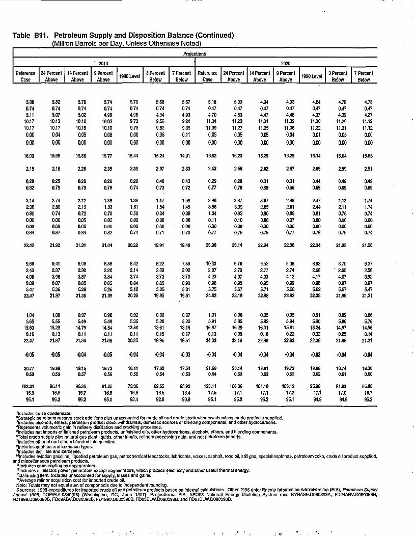
Table B11. Petroleum Supply and Disposition Balance (Continued)(Million Barrels per Day, Unless Otherwise Noted)
Protections
' 2010
Reference
Case
24 Percent
Above
14 Percent
Above
9 Percent
Above1990 Level
3 Percent
Below
7 Percent
Below
2020
Reference
Case
24 Percent
Above
14 Percent
Above
9 Percent
Above1990 Level
3 Percent
Below
7 Percent
Below
5.86
0.74
5.11
10.17
10.17
0,00
0,00
16.03
2.15
0.29
0.82
3.14
2.96
0,95
0.06
0.00
0.84
5.82
0.745.07
10.13
10.17
0,040,00
15.95
2.18
0.25
0.79
2.74
2.80
0.74
0.060.00
0.87
5.76
0.74
5.02
10.10
10.15
0.05
0.00
15.86
2.26
0.28
0.79
2.12
2.19
0.72
0.050.00
0.84
5.74
0.74
4.99
10.03
10.10
0.08
0.00
15.77
2.35
0.28
0.78
1.86
1.93
0.70
0.050.00
0.82
5.70
0.74
4.96
9.73
9.73
0.00
0.00
15.44
2.39
0.28
0.74
1.38
1.61
0.50
0.02
0.00
0.74
5.68
0.74
4.94
9.56
9.62
0.06
0.00
15.24
2.37
0.40
0.73
1.17
1.54
0.34
0.00
0.00
0.71
5.67
0.74
4.93
9.24
9.35
0.11
0.00
14.91
2.33
0.43
0.72
1.09
1.49
0.30
0.00
• 0.00
0.70
5.18
0.47
4.70
11.34
11.39
0.05
0.00
16.52
2.43
0.29
0.77
3.96
3.58
1.04
0.110.00
0.77
5.00
0.47
4.53
11.22
11.27
0.05
0.00
16.23
2.56
0.28
0.70
3.37
3.09
0.93
0.100.00
0.76
4.94
0.47
4.47
11.31
11.35
0.05
0.00
16.25
2.62
0.31
0.69
3.07
2.85
0.90
0.080.00
0.75
4.93
0.47
4.46
11.32
11.36
0.04
0.00
16.25
2.67
0.31
0.66
2.99
2.81
0.88
0.070.00
0.77
4.84
0.47
4.37
11.30
11.32
0.01
0.00
16.14
2.65
0.44
0.65
2.47
2.44
0.81
0.00
0.00
0.79
4.78
0.47
4.32
11.26
11.31
0.05
0.00
16.04
2.59
0.49
0.69
2.12
2.11
0.76
0.000.00
0.75
4.73
0.47
4.27
11.12
11.12
0.000.00
15.85
2.51
0.49
0.69
1.74
1.74
0.74
0.00
0.00
0.74
22.42 21.92 21.31 21.04 20.22 19.91 19.48 23.98 23.14 22.94 22.88 22.34 21.93 21.28
9.66
2,40
4.06
0.89
5.47
22.47
1.04
5.65
15.63
0.16
22.47
9.41
2.37
3.96
0.87
5.36
21.97
1.00
5.55
15.29
0.13
21.97
9.06
2.30
3.87
0.85
5.28
21.36
0.97
5.49
14.79
0.11
21.36
8.88
2.26
3.84
0.85
5.26
21.09
0.96
5.49
14.54
0.11
21.09
8.42
2.14
3.74
0.84
5.12
20.25
0.92
5.35
13.88
0.11
20.25
8.22
2.09
3.73
0.85
5.05
19.95
0.90
5.30
13.61
0.15
19.95
7.89
2.02
3.70
0.90
5.01
19.51
0.87
5.30
13.18
0.17
19.51
10.20
2.87
4.23
0.93
5.75
24.02
1.01
5.91
16.97
0.13
24.02
9.70
2.79
4.07
.0.95
5.67
23.18
0.96
5.85
16.29
0.08
23.18
9.52
2.77
4.03
0.95
5.71
22.98
0.95
5.92
16.01
0.10
22.98
9.38
2.74
4.12
0.99
5.6822.92
0.95
5.94
15.81
0.22
22.92
8.93
2.68
4.17
0.985.62
22.38
0.91
5.90
15.24
0.32
22.38
8.70
" 2.65
4.07
0.97
5.57
21.96
0.89
5.86
14.97
02521.96
8.37
2.58
3.92
0.97
5.47
21.31
0.86
5.76
14.56
0.14
21.31
-0,05 •0,05 -0.04 •0.05 •0.04 •0.04 -0.03 •0.04 -0.04 •0.04 •0.04 •0.03 -0.04 •0.04
20.770.59
103.21
16.9
95.1
19.990.59
96.11
16.8
95.2
19.150.57
86.36
16.7
95.2
18.720.56
81.85
16.6
95.0
18.110.55
73.36
16.6
93.4
17.820.54
69.65
16.5
92.8
17.540.53
65.92
16.4
90.9
21.690.64
123.11
17.5
95.1
20.140.63
108.06
17.195.2
19.810.63
104.10
17.1
95.2
19.730.62
103.1217595.1
19.080.62
95.98
17.1
94.9
18.740.61
91.83
17.0
94.9
18.380.60
85.88
16.7
955
'Includes lease condensate.'Strategic petroleum reserve stock additions plus unaccounted for crude oil and crude stock withdrawals minus crude products supplied.'Includes alcohols, ethers, petroleum product stock withdrawals, domestic sources of blending components, and other hydrocarbons.'Represents volumetric gain in refinery distillation and cracking processes.'Includes net imports of finished petroleum products, unfinished oils, other hydrocarbons, alcohols, ethers, and blending components.'Total crude supply plus natural gas plant liquids, other inputs, refinery processing gain, and net petroleum imports.'Includes ethanol and ethers blended into gasoline.'Includes naphtha and kerosene types.'Includes distillate and kerosene."Includes aviation gasoline, liquefied petroleum gas, petrochemical feedstocks, lubricants, waxes, asphalt, road oil, still gas, special naphthas, petroleum coke, crude oil product supplied,
and miscellaneous petroleum products."Includes consumption by cogenerators."Includes all electric power generators except cogenerators, which produce electricity and other useful thermal energy."Balancing item. Includes unaccounted for supply, losses and gains."Average refiner acquisition cost for imported crude oil.Note: Totals may not equal sum of components due to independent rounding.Sources: 1996 expenditures for imported crude oil and petroleum products based on internal calculations. Other 1996 data: Energy Information Administration (EIA), Petroleum Supply
Annual 1996, DOE/EIA-0340(96) (Washington, DC, June 1997). Projections: EIA, AEO98 National Energy Modeling System runs KYBASE.D080398A, FD24ABV.D080398B,FD1998.D080398B, FD09ABV.D080398B, FD1990.D080398B, FD03BLW.D080398B, and FD07BLW.D080398B.

Table B12. Petroleum Product Prices(1996 Cents per Gallon Unless Otherwise Noted)
Sector and Fuel 1996
Projections
2005
Reference
Case
24 Percent
Above
14 Percent
Above
9 Percent
Above1990 Level
3 Percent
Below
7 Percent
Below
World Oil Price (1996 dollars per barrel) 20.48
Delivered Sector Product Prices
ResidentialDistillate Fuel 98.4
Liquefied Petroleum Gas 100.0
Commercial
Distillate Fuel 73.1
Residual Fuel 48.4
Residual Fuel (1996 dollars per barrel) 20.35
Industrial'
Distillate Fuel 76.3
Liquefied Petroleum Gas 67.3
Residual Fuel 44.8
Residual Fuel (1996 dollars per barrel) 18.81
Transportation
Diesel Fuel (distillate)2 123.5
Jet Fuel3 74.6
Motor Gasoline' 122.5
Liquefied Petroleum G a s . . . : 109.0
Residual Fuel 38.2
Residual Fuel (1996 dollars per barrel) 16.04
E85 141.7
M85 89.6
Electric Generators5
Distillate Fuel 68.1
Residual Fuel 45.9
Residual Fuel (1996 dollars per barrel) 19.28
Refined Petroleum Product Prices6
Distillate Fuel 108.7
Jet Fuel3 74.6
Liquefied Petroleum Gas 73.6
Motor Gasoline4 122.5
Residual Fuel 42.5
Residual Fuel (1996 dollars per barrel) 17.87
Average 102.8
20.26 20.12 20.04 19.96 19.95 19.91 19.89
105.3
104.5
74.5
46.0
19.31
75.3
57.9
41.1
17.28
117.4
72.5
123.0
112.1
40.5
17.00
146.2
91.8
68.9
46.4
19.49
107.0
72.5
68.1
122.8
42.0
17.64
101.9
106.5
105.5
75.8
47.8
20.09
76.7
58.9
42.6
17.88
119.5
74.4
125.1
113.1
41.8
17.58
146.5
92.3
70.7
47.2. 19.81
109.0
74.4
69.2
124.9
43.3
18.20
103.7
117.6
111.1
87.061.8
25.97
88.0
64.3
56.4
23.68
130.5
85.1
134.2
118.6
55.6
23.36
148.4
97.6
82.2
61.6
25.86
120.1
85.1
74.6
134.0
57.2
24.01
113.0
124.8
114.1
94.2
70.0
29.39
95.2
67.3
64.9
27.27
137.2
91.6
140.6
121.5
64.3
27.00
149.2
100.9
89.5
70.4
29.58
126.9
91.6
77.5
140.4
65.8
27.63
119.0
127.6
115.5
96.9
73.3
30.77
97.8
68.8
68.2
28.62
139.7
94.0
143.1
122.9
67.4
28.32
149.6
102.2
92.2
74.1
31.14
129.4
94.0
79.0
142.9
69.0
28.98
121.4
129.7
116.7
99.075.8
31.82
100.1
69.9
70.7
29.70
141.9
96.0
144.9
124.0
70.0
29.40
149.8
103.2
94.5
76.7
32.19
131.7
96.0
80.1
144.7
71.5
30.03
123.2
132.0
117.9
101.4
78.5
32.95
102.4
71.1
73.4
30.84
• 144.1
98.0
146.8
125.2
72.5
30.45
150.1
104.2
96.9
79.1
33.23
133.9
98.0
81.3
146.6
74.1
31.13
125.0
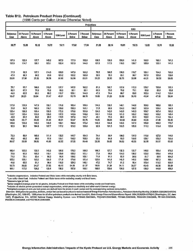
Table B12. Petroleum Product Prices (Continued)(1996 Cents per Gallon Unless Otherwise Noted)
Prelections
2010
Reference
Case
24 Percent
Above
14 Percent
Above
9 Percent
Above1990 Level
3 Percent
Below
7 Percent
Below
2020
Reference
Case
24 Percent
Above
14 Percent
Above
9 Percent
Above1990 Level
3 Percent
Below
7 Percent
Below
20.77 19.99 19.15 18.72 18.11 17.82 17.54 21.69 20.14 19.81 19.73 19.08 18.74 18.38
107.9
107.9
77.3
47.6
20.01
78,7
60.5
44.0
18.47
117,875.8
125.4
113.743.5
18.25
149,692.5
7Z349.2
20,67
108,4
75,8
71.5
125,2
44.6
18,73
104.1
122.9
114.7
92.3
66.3
27.86
93.7
67.2
62.5
26.23
132.9
90.3
139.3
120.462.3
26.17
150.2
99.1
88.0
69.2
29.08
123.5
90.3
78.1
139.1
63.5
26.65
117.0
137.7
120.1
107.1
84.2
35,35
108.6
72.6
80.1
33.64
147.9
103.3
150.4125.6
80.0
33.59
146.5104.8
103.6
88.0
36.95
138.5
103.3
83.4 •
150.2
81.1
34.07
128.2
145.2
123.1
114.5
93.8
39.38
115.8
75.6
89.2
37.47
155.1
110.1
155.5
128.689.2
37.45
146.5
107.7
111.4
97.6
41.00
145.6
110.1
86.3
155.3
90.4
37.95
133.4
167.9
132.4
136.9
121.2
50.90
137.7
85.0
115.7
48.61
175.6
129.8
172.0
137.5115.5
48.51
162.1
117.2
132.5
125.1
52.52
166.6
129.8
95.6
171.8
116.9
49.10
150.0
177.9
137.5
147.0
133.2
55.96
147.9
90.1
128.1
53.79
185.4
138.3
179.8
142.6127.8
53.67
168.4121.5
140.7
136.3
57.25
176.3
138.3
100.5
179.6
129.3
54.29
157.8
192.0
144.9
161.2
150.0
63.01
162.2
98.1
144.5
60.70
199.5
151.1
191.6
149.8144.7
60.76
175.4
126.0
154.5
153.3
64.40
190.3
151.1
108.1
191.4
146.1
61.37
169.1
108.5
107.8
78.5
50.5
21.23
81.3
60.3
47.3
19.86
114.0
77.8
124.0110.1
46.1
19.35
148.392.9
74.4
53522.36
106.3
77.8
71.8
123.9
47.2
19.81
102.9
130.9
117.5
100.5
78.3
32.90
102.7
70.0
74.4
31.26
135.2
98.9
142.0
119.873.6
30.93
144.8
101.5
96.9
84.8
35.62
127.7
98.9
81.5
141.8
74.7
31.39
120.6
136.9
118.5
106.0
85.1
35.75
107.6
70.6
80.7
33.89
140.1
104.0
145.5121.080.2
33.68
145.5
103.5
100.0
93.3
39.20
132.3
104.0
825145.3
81534.11
124.0
141.6
120.7
110.7
90.7
38.08
112.3
73.1
85.9
36.10
144.6
108.2
149.3
123585.3
35.83
147.9
105.6
104.3
100.6
42.25
135.7
108.2
84.6
149.2
86.4
36.27
127.5
155.9
128.0
125.1
107.9
45.31
126.7
80.8
102.5
43.04
159.5
122.0
159.7
1305
102.5
43.05
155.9
111.2
118.6
120.7
50.68
149.5
122.0
91.7
159.6
103.4
43.43
138.3
165.1
133.1
134.3
120.0
50.38
135.9
85.9
114.2
47.95
168.9
130.5
167.4135.2
114.3
47.99
160.3
115.4
127.8
132.3
55.57
159.4130.596.6
167.3115548.39146.0
181.2
141.5
150.5
139.6
58.65
152.1
93.8
133.4
56.04
185.1
144.9
180.2143.4
134.1
56.32
170.7
122.6
144.0
150.5
63.22
176.5
144.9
104.5
180.1
135.0
56.69
158.9
'Includes cogeneralors. Includes Federal and State taxes while excluding county and state taxes.'Low sulfur dlesel fuel. Includes Federal and State taxes while excluding county and local taxes.'Kerosene-type Jet fuel.4Sales weighted-average price for all grades. Includes Federal and State taxes while excluding county and local taxes.'Includes all electric power generators except cogeneralors, which produce electricity and other useful thermal energy.'Weighted averages of end-use fuel prices are derived from the prices in each sector and the corresponding sectoral consumption.
Sources: 1996 prices for gasoline, distillate, and jet fuel are based on prices in various issues of Energy Information Administration, Petroleum Marketing Monthly, DOE/EIA-0380(96/03-97/04)(Washington, DC, 1996-97). 1996 prices for all other petroleum products are derived from El A, State Energy Price and Expenditures Report: 1994, DOE/E!A-0376(94) (Washington, DC, June1997). Projections: EIA, AEO98 National Energy Modeling System runs KYBASE.D080398A, FD24ABV.D080398B, FD1998.D080398B, FD09ABV.D080398B, FD1990.D080398B,FD03BLW.D080398B, and FD07BLW.D080398B.
Energy Information Administration / Impacts of the Kyoto Protocol on U.S. Energy Markets and Economic Activity . 195
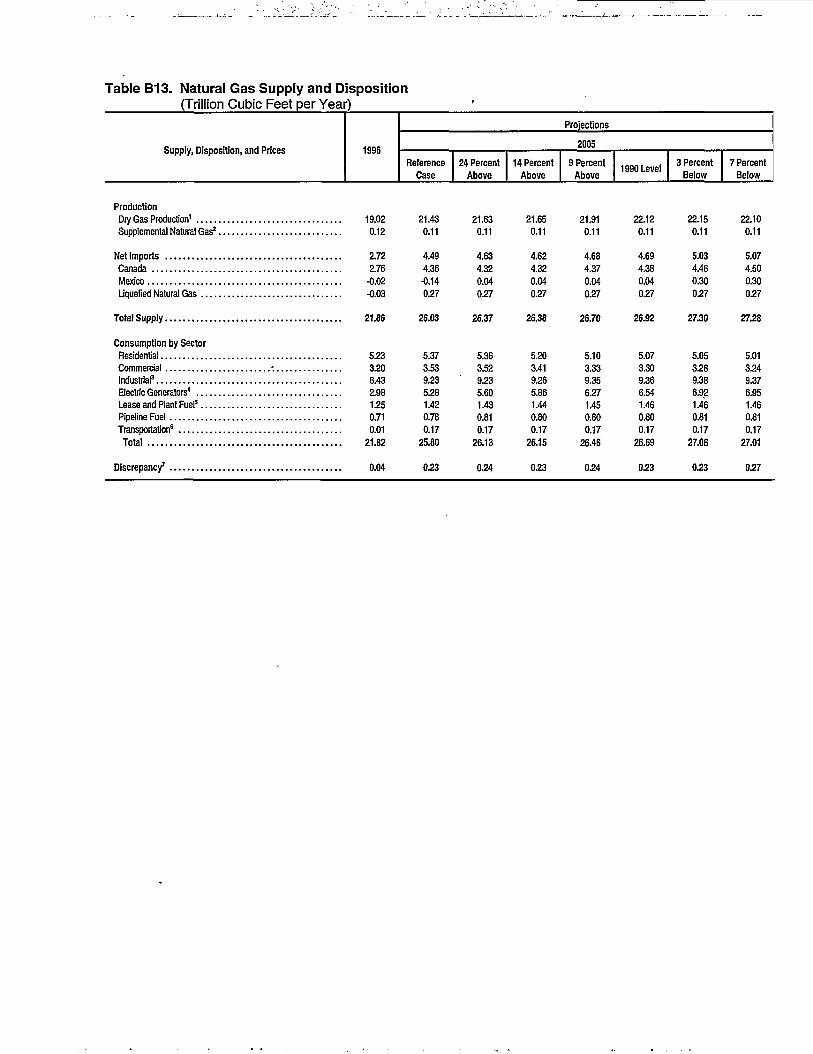
Table B13. Natural Gas Supply and Disposition(Trillion Cubic Feet per Year)
Supply, Disposition, and Prices 1996
Projections
2005
ReferenceCase
24 PercentAbove
14 PercentAbove
9 PercentAbove
1990 Level 3 PercentBelow
7 PercentBelow
ProductionDry Gas Production1 19.02Supplemental Natural Gas2 0.12
Netlmports 2.72Canada 2.76Mexico -0.02Liquefied Natural Gas -0.03
Total Supply 21.86
Consumption by SectorResidential 5.23Commercial •. 3.20Industrial3 8.43Electric Generators4 2.98Lease and Plant Fuel5 1.25Pipeline Fuel 0.71Transportation6 0.01Total 21.82
Discrepancy7 0.04
21.430.11
4.494.36
-0.140.27
21.630.11
4.634.320.040.27
21.650.11
4.624.320.040.27
21.910.11
4.684.370.040.27
22.120.11
4.694.380.040.27
22.150.11
5.034.460.300.27
22.100.11
5.074.500.300.27
26.03
0.23
26.37
0.24
26.38 26.70 26.92
0.23 0.24 0.23
27.30
0.23
27.28
5.373.539.235.281.420.780.17
25.80
5.363.529.235.601.430.810.17
26.13
5.203.419.265.861.440.800.17
26.15
5.103.339.356.271.450.800.17
26.46
5.073.309.366.541.460.800.17
26.69
5.053.289.386.921.460.810.17
27.06
5.013.249.376.951.460.810.17
27.01
0.27
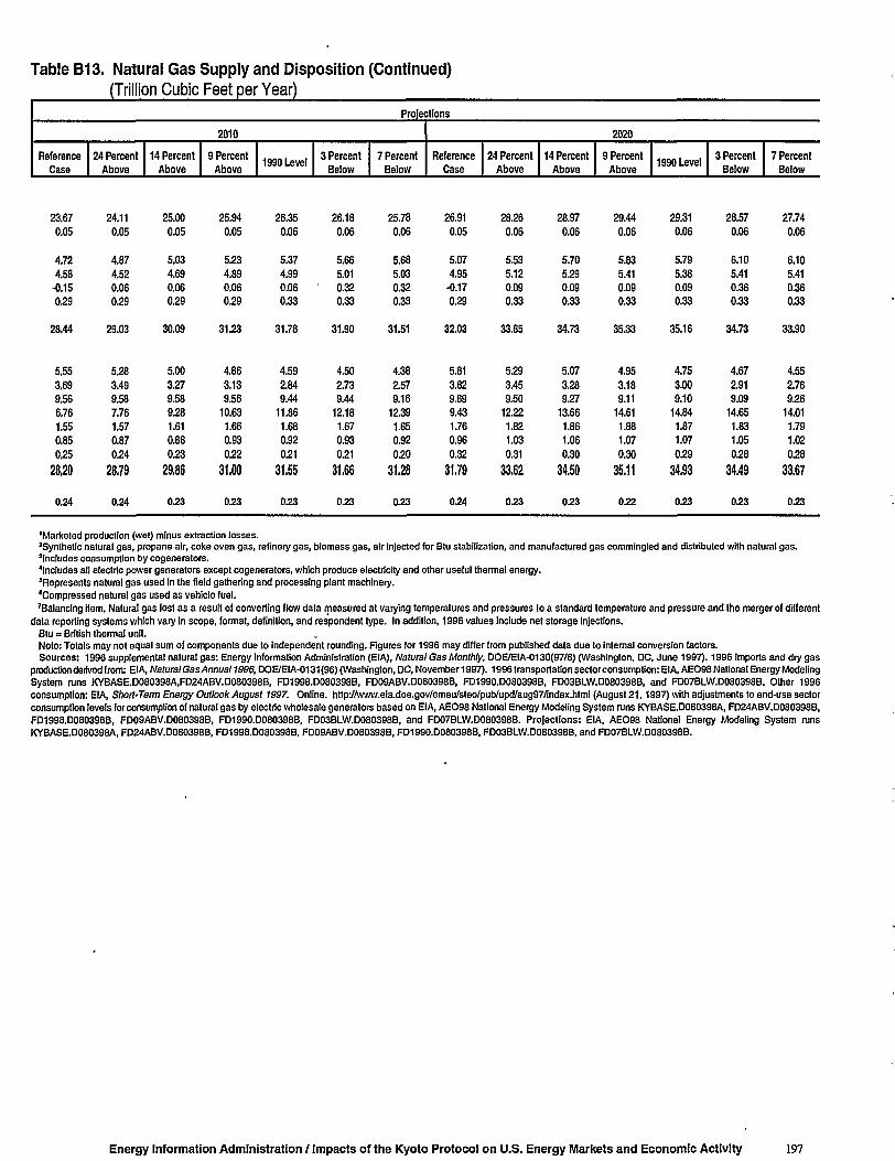
Table B13. Natural Gas Supply and Disposition (Continued)(Trillion Cubic Feet per Year)
Projections
2010
Reference
Case
24 Percent
Above
14 Percent
Above
9 Percent
Above1990 Level
3 Percent
Below
7 Percent
Below
2020
Reference
Case
24 Percent
Above
14 Percent
Above
9 Percent
Above1990 Level
3 Percent
Below
7 Percent
Below
23.67
0.05
4,72
4.58
-0.15
0.29
24.11
0.05
4.87
4.52
0.06
0.29
25.00
0.05
5.03
4.69
0.06
0.29
25.94
0.05
5.23
4.89
0.06
0.29
26.35
0.06
5.37
4.99
0.06
0.33
26.18
0.06
5.66
5.01
• 0.32
0.33
25.78
0.06
5.68
5.03
0.32
0.33
26.91
0.05
5.07
4.95
•0.17
0.29
28.26
0.06
5.53
5.12
0.09
0.33
28.97
0.06
5.70
5.29
0.09
0.33
29.44
0.06
5.83
5.41
0.09
0.33
29.31
0.06
5.79
5.38
0.09
0.33
28.57
0.06
6.10
5.41
0.36
0.33
27.74
0.06
6.10
5.41
0.36
0.33
28.44 29.03 30.09 31.23 31.78 31.90 31.51 32.03 33.85 34.73 35.33 35.16 34.73 33.90
5.55
3.69
9.56
6.76
1.55
0.85
0.25
28,20
0.24
5.28
3.49
9.58
7.76
1.57
0.87
0.24
28,79
0.24
5.00
3.27
9.58
9.28
1.61
0.88
0.23
29.86
0.23
4.86
3.13
9.56
10.63
1.66
0.93
0.22
31.00
023
4.59
2.84
9.44
11.86
1.68
0.92
0.21
31.55
023
4.50
2.73
9.44
12.18
1.67
0.93
0.21
31.66
023
4.38
2.57
9.16
12.39
1.65
0.92
0.20
31.28
023
5.81
3.82
9.69
9.43
1.76
0.96
0.32
31.79
024
5.29
3.45
9.50
12.22
1.82
1.03
0.31
33.62
023
5.07
3.28
9.27
13.66
1.86
1.06
0.30
34.50
023
4.95
3.18
9.11
14.61
1.88
1.07
0.30
35.11
022
4.75
3.00
9.10
14.84
1.87
1.07
0.29
34.93
023
4.67
2.91
9.09
14.65
1.83
1.05
0.28
34.49
023
4.55
2.76
9.26
14.01
1.79
1.02
0.28
33.67
023
'Marketed production (wet) minus extraction losses.'Synthetic natural gas, propane air, coke oven gas, refinery gas, biomass gas, air injected for Btu stabilization, and manufactured gas commingled and distributed with natural gas.'Includes consumption by cogenerators.'Includes all electric power generators except cogenerators, which produce electricity and other useful thermal energy.'Represents natural gas used In the field gathering and processing plant machinery.'Compressed natural gas used as vehicle fuel.'Balancing Item. Natural gas lost as a result of converting flow data measured at varying temperatures and pressures to a standard temperature and pressure and the merger of different
data reporting systems which vary In scope, format, definition, and respondent type. In addition, 1996 values include net storage injections.Btu = British thermal unit.Note: Totals may not equal sum of components due to independent rounding. Figures for 1996 may differ from published data due to internal conversion factors.Sources: 1996 supplemental natural gas: Energy Information Administration (EIA), Natural Gas Monthly, DOE/EIA-0130(97/6) (Washington, DC, June 1997). 1996 imports and dry gas
production derived from: EIA,/vafura/Gas/ln/7ua/79S5,DOE/EIA-0131(96) (Washington, DC, November 1997). 1996 transportation sector consumption: EIA, AEO98 National Energy ModelingSystem runs KYBASE.D080398A,FD24ABV.D080398B, FD1998.D080398B, FD09ABV.D080398B, FD1990.D080398B, FD03BLW.D080398B, and FD07BLW.D080398B. Other 1996consumption: EIA, Short'Term Energy Outlook August 1997. Online, http://www.eia.doe.gov/emeu/steo/pub/upd/aug97/index.html (August 21,1997) with adjustments to end-use sectorconsumption levels for consumption of natural gas by electric wholesale generators based on EIA, AEO98 National Energy Modeling System runs KYBASE.D080398A, FD24ABV.D080398B,FD1998.D080398B, FD09ABV.D080398B, FD1990.D080398B, FD03BLW.D080398B, and FD07BLW.D080398B. Projections: EIA, AEO98 National Energy Modeling System runsKYBASE.D080398A, FD24ABV.D080398B, FD1998.D080398B, FD09ABV.D080398B, FD1990.D080398B, FD03BLW.D080398B, and FD07BLW.D080398B.
Energy Information Administration / Impacts of the Kyoto Protocol on U.S. Energy Markets and Economic Activity 197
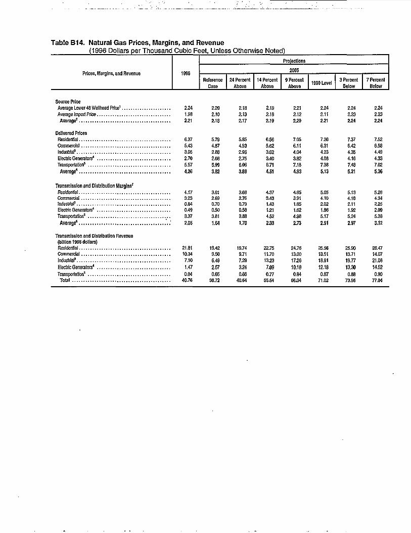
Table B14. Natural Gas Prices, Margins, and Revenue(1996 Dollars per Thousand Cubic Feet, Unless Otherwise Noted)
Prices, Margins, and Revenue 1996
Projections
2005
Reference
Case
24 Percent
Above
14 Percent
Above
9 Percent
Above1990 Level
3 Percent
Below
7 Percent
Below
Source PriceAverage Lower 48 Wellhead Price1 2.24
Average Import Price 1.98
Average2 2.21
Delivered Prices
Residential 6.37
Commercial 5.43Industrial3 3.05
Electric Generators' 2.70
Transportation5 5.57
Average6 4.26
Transmission and Distribution Margins7
Residential 4.17
Commercial 3.23Industrial3 0.84
Electric Generators* 0.49
Transportation' 3.37
Average6 ' 2.05
Transmission and Distribution Revenue
(billion 1996 dollars)
Residential 21.81
Commercial 10.34Industrial3 7.10Electric Generators4 1.47Transportation5 0.04
Total 40.76
2.20
2.10
2.18
5.79
4.87
2.88
2.68
5.99
3.82
3.612.690.70
0.50
3.81
1.64
19.42
9.50
6.49
2.670.65
38.72
2.18
2.13
2.17
5.85
4.93
2.96
2.75
6.06
3.88
3.682.760.79
0.58
3.88
1.70
19.74
9.71
7.29
3.240.66
40.64
2.19
2.18
2.19
6.56
5.62
3.62
3.40
6.71
4.51
4.373.431.43
1.21
4.52
2.33
22.75
11.70
13.23
7.09
0.77
55.54
2.21
2.12
2.20
7.05
6.11
4.04
3.82
7.18
4.93
4.853.911.85
1.62
4.98
2.73
24.76
13.00
17.26
10.180.84
66.04
2.24
2.11
2.21
7.26
6.31
4.23
4.08
7.38
5.13
5.054.102.02
1.86
5.17
2.91
25.56
13.51
18.91
12.180.87
71.02
2.24
2.23
254
7.37
6.42
4.35
4.16
7.48
5.21
5.134.182.11
1.92
5.24
2.97
25.90
13.71
19.77
13.300.88
73.56
2.24
2.23
2.24
7.52
6.58
4.49
4.33
7.62
5.36
5.284.34
2.25
2.09
5.38
3.12
26.47
14.07
21.08
14.520.90
77.04
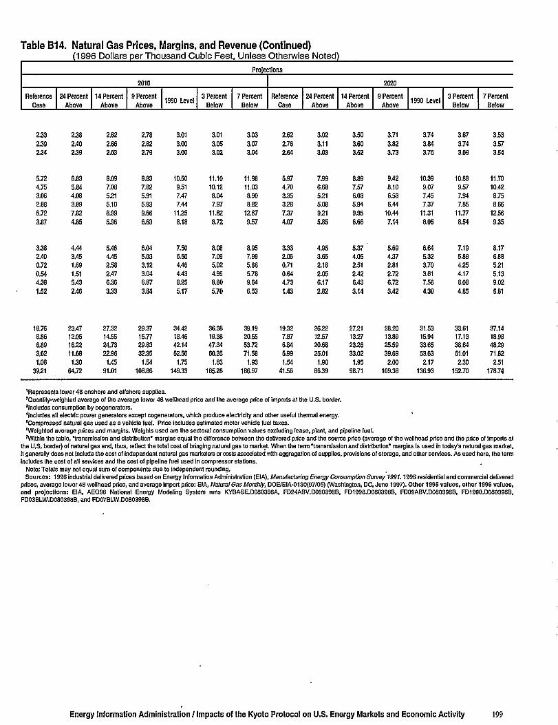
Table B14. Natural Gas Prices, Margins, and Revenue (Continued)(1996 Dollars per Thousand Cubic Feet, Unless Otherwise Noted)
Projections
2010
Reference
Case
2.33
2.39
2.34
5.72
4.75
3.06
2.88
6.72
3.87
3.38
2.40
0.72
0,54
4,38
1.52
24 Percent
Above
2.38
2.40
2.39
6.83
5.84
4.08
3.89
7.82
4.85
4.44
3.45
1.69
1.51
5.43
2.46
14 Percent
Above
2.62
2.66
2.63
8.09
7.08
5.21
5.10
8.99
5.96
5.46
4.45
2.58
2.47
6.36
3.33
9 Percent
Above
2.78
2.82
2.79
8.83
7.82
5.91
5.83
9.66
6.63
6.04
5.03
3.12
3.04
6.87
3.84
1990 Level
3.01
3.00
3.00
10.50
9.51
7.47
7.44
11.25
8.18
7.50
6.50
4.46
4.43
8.25
5.17
3 Percent
Below
3.01
3.05
3.02
11.10
10.12
8.04
7.97
11.82
8.72
8.08
7.09
5.02
4.95
8.80
5.70
7 Percent
Below
3.03
3.07
3.04
11.98
11.03
8.90
8.82
12.67
9.57
8.95
7.99
5.86
5.78
9.64
6.53
2020
Reference
Case
2.62
2.76
2.64
5.97
4.70
3.35
3.28
7.37
4.07
3.33
2.06
0.71
0.64
4.73
1.43
24 Percent
Above
3.02
3.11
3.03
7.99
6.68
5.21
5.08
9.21
5.85
4.95
3.65
2.18
2.05
6.17
2.82
14 Percent
Above
3.50
3.60
3.52
8.89
7.57
6.03
5.94
9.95
6.66
5.37 '
4.05
£512.42
6.43
3.14
9 Percent
Above
3.71
3.82
3.73
9.42
8.10
6.53
6.44
10.44
7.14
5.69
4.37
2.81
2.72
6.72
3.42
1990 Level
3.74
3.84
3.76
10.39
9.07
7.45
7.37
11.31
8.05
6.64
5.32
3.70
3.61
7.56
4.30
3 Percent
Below
3.67
3.74
3.69
10.88
9.57
7.94
7.85
11.77
8.54
7.19
5.89
4.25
4.17
8.08
4.85
7 Percent
Below
3.53
3.57
3.54
11.70
10.42
8.75
8.66
12.56
9.35
8.17
6.88
5.21
5.13
9.02
5.81
18.76
8.86
6.89
3.62
1.08
39.21
23.4712.05
16.22
11.68
1.30
64.72
27.32
14.55
24.73
22.96
1.45
91.01
29.37
15.77
29.83
32.35
1.54
108.86
34.4218.46
42.14
52.56
1.75
149.33
36.38
19.38
47.34
60.35
1.83
165.28
39.19
20.55
53.72
71.58
1.93
186.97
19.32
7.87
6.84
5.99
1.54
41.56
262212.57
20.68
25.01
1.90
86.39
27.211327232633.02
1.95
98.71
28.20
13.89
25.59
39.69
2.00
109.38
31.53
15.94
33.65
53.63
2.17
136.93
33.61
17.13
38.64
61.01
2.30
152.70
37.14
18.98
48.29
71.82
2.51
178.74
'Represents lov/er 48 onshore and offshore supplies.'Quantity-weighted average of the average lower 48 wellhead price and the average price of imports at the U.S. border.'Includes consumption by cogenerators.'Includes all electric power generators except cogenerators, which produce electricity and other useful thermal energy."Compressed natural gas used as a vehicle fuel. Price includes estimated motor vehicle fuel taxes.'Weighted average prices and margins. Weights used are the sectoral consumption values excluding lease, plant, and pipeline fuel.'Within the table, 'transmission and distribution" margins equal the difference between the delivered price and the source price (average of the wellhead price and the price of imports at
the U.S. border) of natural gas and, thus, reflect the total cost of bringing natural gas to market. When the term 'transmission and distribution' margins is used in today's natural gas market,It generally does not include the cost of independent natural gas marketers or costs associated with aggregation of supplies, provisions of storage, and other services. As used here, the termIncludes the cost of all services and the cost of pipeline fuel used in compressor stations.
Note; Totals may not equal sum of components due to independent rounding.Sources: 1996 industrial delivered prices based on Energy Information Administration (EIA), Manufacturing Energy Consumption Survey 1991.1996 residential and commercial delivered
prices, average lov/er 48 v/ellhead price, and average import price: EIA, Natural Gas Monthly, DOE/EIA-0130(97/06) (Washington, DC, June 1997). Other 1995 values, other 1996 values,and projections: EIA, AEO98 National Energy Modeling System runs KYBASE.D080398A, FD24ABV.D080398B, FD1998.D080398B, FD09ABV.D080398B, FD1990.D080398B,FD03BLW.D080398B, and FD07BLW.D080398B.
Energy Information Administration / Impacts of the Kyoto Protocol on U.S. Energy Markets and Economic Activity 199
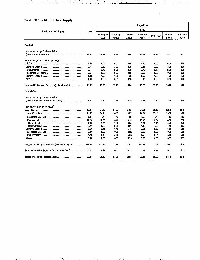
Table B15. Oil and Gas Supply
Production and Supply 1996
Projections
2005
Reference
Case
24 Percent
Above
14 Percent
Above
9 Percent
Above1990 Level
3 Percent
Below
7 Percent
Below
Crude Oil
Lower 48 Average Wellhead Price1
(1996 dollars per barrel) 19.41
Production (million barrels per day)2
U.S.Total 6.48
Lower 48 Onshore 3.76
Conventional 3.15
Enhanced Oil Recovery 0.61
Lower 48 Offshore 1.32
Alaska 1.40
Lower 48 End of Year Reserves (billion barrels) 16.82
Natural Gas
Lower 48 Average Wellhead Price1
(1996 dollars per thousand cubic feet) 2.24
Production (trillion cubic feet)3
U.S.Total 19.01
Lower 48 Onshore 13.07
Associated-Dissolved' 1.84
Non-Associated 11.23Conventional 7.96Unconventional 3.27
Lower 48 Offshore 5.50
Associated-Dissolved* 0.80
Non-Associated 4.70
Alaska 0.43
Lower 48 End of Year Reserves (trillion cubic feet) 157.23
Supplemental Gas Supplies (trillion cubic feet)5 0.12
Total Lower 48 Wells (thousands) 22.07
19.78
15.28
2.20
19.69
1525
2.18
19.54 < 19.44 19.39 19.32 19.31
6.023.392.760.631.690.93
6.013.392.750.631.690.93
6.003.382.750.631.690.93
6.003.382.750.631.690.93
6.003.382.750.631.680.93
6.003.382.750.631.680.93
6.003.382.750.631.690.93
1554
2.19
15.23
2.21
15.23
2.24
15.22
2.24
15.23
2.24
21.43
14.49
1.5312.969.093.886.41
0.92
5.49
0.53
172.31
0.11
28.12
21.63
14.68
1.5213.169.173.996.42
0.92
5.50
0.53
171.86
0.11
28.06
21.65
14.67
1.5213.159.243.916.45
0.92
5.53
0.53
171.61
0.11
28.08
21.91
14.87
1.5213.359.344.02
6.51
0.92
5.59
0.53
171.58
0.11
28.04
22.12
15.06
1.5213.549.454.09
6.53
0.92
5.61
0.53
171.03
0.11
28.06
22.15
15.13
1.52
13.609.434.186.500.92
5.58
0.53
170.87
0.11
28.16
22.10
15.02
1.52
13.509.434.076.55
0.92
5.63
0.53
171.25
0.11
28.15
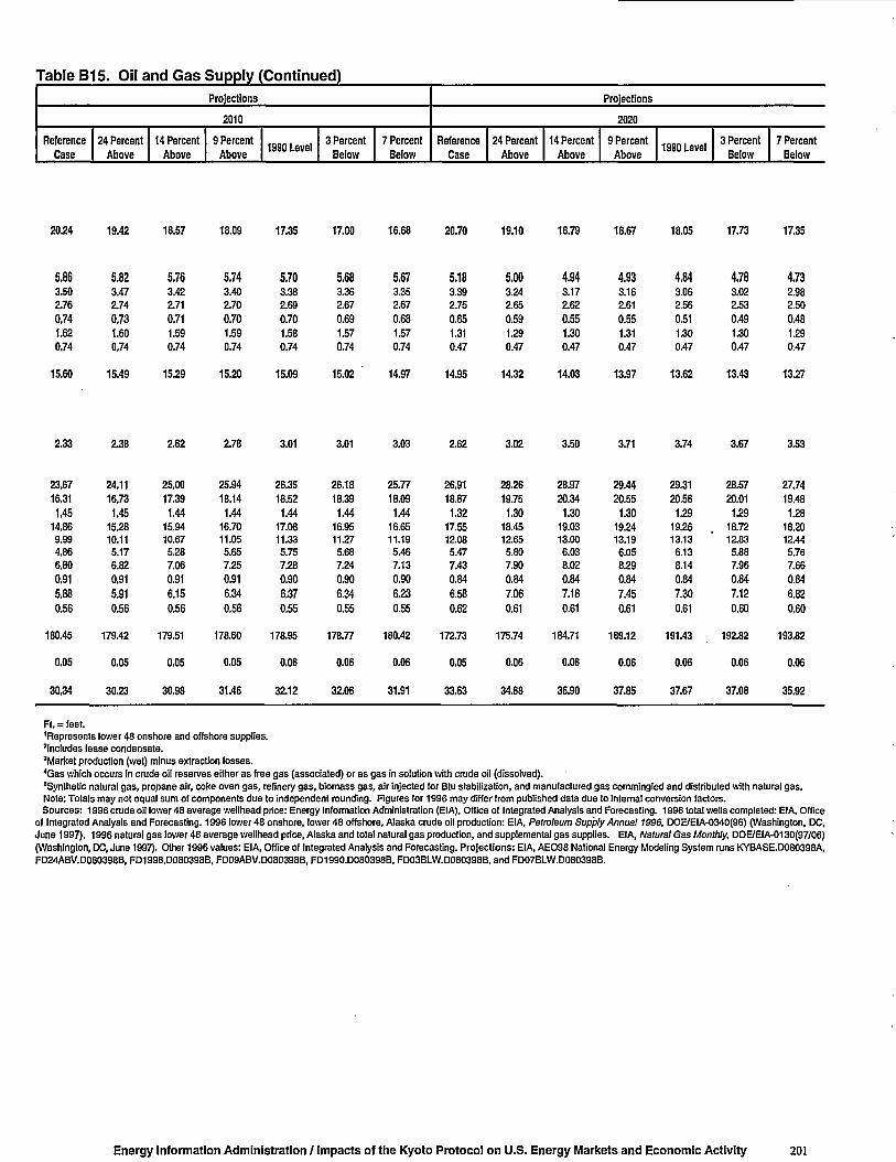
Table B15. Oil and Gas Supply (Continued)Projections
2010
Reference
Case
24 Percent
Above
14 Percent
Above
9 Percent
Above1990 Level
3 Percent
Below
7 Percent
Below
Projections
2020
Reference
Case
24 Percent
Above
14 Percent
Above
9 Percent
Above1990 Level
3 Percent
Below
7 Percent
Below
20.24 19.42 18.57 18.09 17.35 17.00 16.68 20.70 19.10 18.79 18.67 18.05 17.73 17.35
5.863.50
2.76
0,74
1.62
0,74
5.823.47
2.74
0,73
1.60
0.74
5.763.42
2.71
0.71
1.59
0.74
5.743.40
2.70
0.70
1.59
0.74
5.703.38
2.69
0.70
1.58
0.74
5.683.36
2.67
0.69
1.57
0.74
5.673.35
2.67
0.68
1.57
0.74
5.183.39
2.75
0.65
1.31
0.47
5.003.24
2.65
0.59
1.29
0.47
4.943.17
2.62
0.55
1.30
0.47
4.933.16
2.61
0.55
1.31
0.47
4.843.06
2.56
0.51
1.30
0.47
4.783.02
2.53
0.49
1.30
0.47
4.732.98
2.50
0.48
1590.47
15.60 15.49 15.29 15.20 15.09 15.02 14.97 14.95 14.32 14.03 13.97 13.62 13.43 13.27
2.33 2.38 2.62 2.78 3.01 3.01 3.03 2.62 3.02 3.50 3.71 3.74 3.67 3.53
23.67
16,31
1.45
14.869.994.86
6.80
0.91
5,88
0.56
180.45
0.05
30.34
24.11
16.73
1.45
15.2810.115.17
6.82
0.91
5,91
0.56
179.42
0.05
30.23
25.00
17.39
1.44
15.9410.675.28
7.06
0.91
6.15
0.56
179.51
0.05
30.98
25.94
18.14
1.44
16.7011.055.65
7.25
0.91
6.34
0.56
178.60
0.05
31.46
26.35
18.52
1.44
17.0811.33
5.75
7.28
0.90
6.37
0.55
178.95
0.06
32.12
26.18
18.39
1.44
16.9511.275.68
7.24
0.90
6.34
0.55
178.77
0.06
32.06
25.77
18.09
1.44
16.6511.195.46
7.13
0.90
6.23
0.55
180.42
0.06
31.91
26.91
18.87
1.32
17.5512.085.47
7.43
0.84
6.58
0.62
172.73
0.05
33.63
28.26
19.75
1.30
18.4512.655.80
7.90
0.84
7.06
0.61
175.74
0.06
34.68
28.97
20.34
1.30
19.0313.006.03
8.02
0.84
7.18
0.61
184.71
0.06
36.90
29.44
20.55
1.30
195413.196.05
8590.84
7.45
0.61
189.12
0.06
37.85
29.31
20.56
1.29
19.2613.136.13
8.14
0.84
7.30
0.61
191.43
0.06
37.67
28.57
20.01
1.29
18.7212.835.88
7.96
0.84
7.12
0.60
192.82
0.06
37.08
27.74
19.48
1.28
185012.445.76
7.66
0.84
6.82
0.60
193.82
0.06
35.92
Ft. = feet.'Represents lov/er 48 onshore and offshore supplies.'Includes lease condensate.'Market production (wet) minus extraction losses.'Gas which occurs in crude oil reserves either as free gas (associated) or as gas in solution with crude oil (dissolved).'Synthetic natural gas, propane air, coke oven gas, refinery gas, biomass gas, air injected for Btu stabilization, and manufactured gas commingled and distributed with natural gas.Note: Totals may not equal sum of components due to independent rounding. Figures for 1996 may differ from published data due to internal conversion factors.Sources: 1996 crude oil lower 48 average wellhead price: Energy Information Administration (EIA), Office of Integrated Analysis and Forecasting. 1996 total wells completed: EIA, Office
of Integrated Analysis and Forecasting. 1996 lov/er 48 onshore, lower 48 offshore, Alaska crude oil production: EIA, Petroleum Supply Annual 1996, DOE/EIA-0340(96) (Washington, DC,June 1997). 1996 natural gas lov/er 48 average v/ellhead price, Alaska and total natural gas production, and supplemental gas supplies. EIA, Natural Gas Monthly, DOE/EIA-0130(97/06)(Washington, DC, June 1997). Other 1996 values: EIA, Office of Integrated Analysis and Forecasting. Projections: EIA, AEO98 National Energy Modeling System runs KYBASE.D080398A,FD24ABV.D080398B, FD1998.D080398B, FD09ABV.D080398B, FD1990.D080398B, FD03BLW.D080398B, and FD07BLW.D080398B.
Energy Information Administration / Impacts of the Kyoto Protocol on U.S. Energy Markets and Economic Activity 201
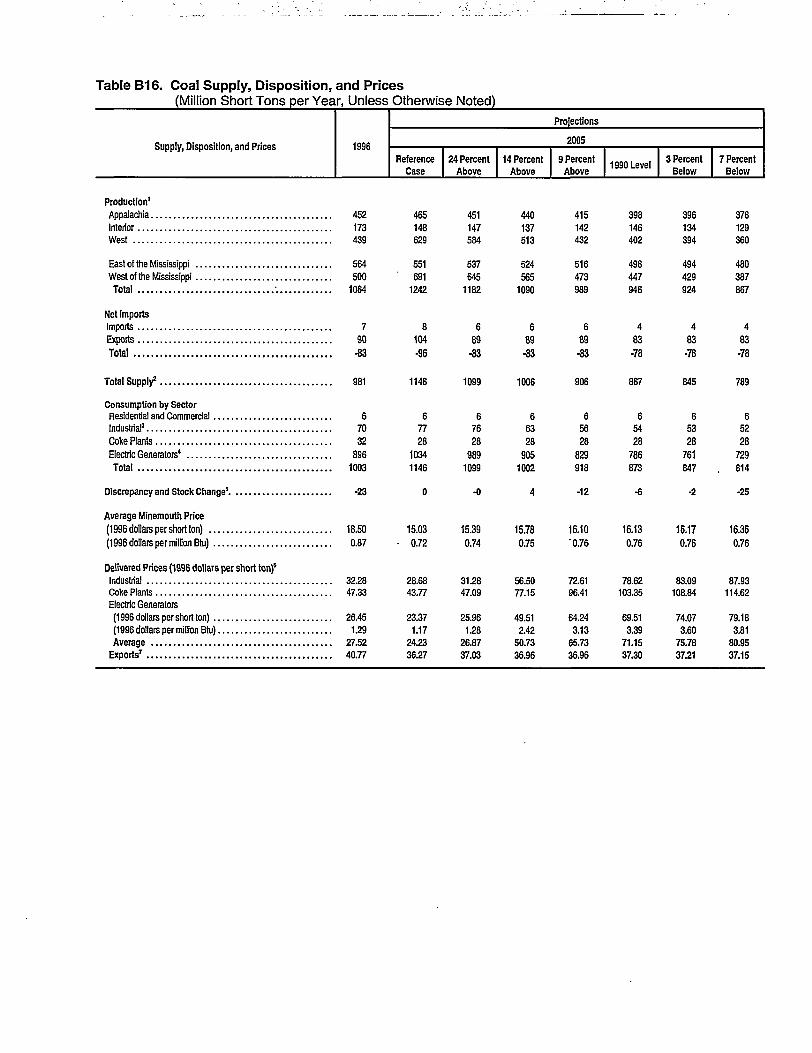
Table B16. Coal Supply, Disposition, and Prices(Million Short Tons per Year, Unless Otherwise Noted)
Supply, Disposition, and Prices 1996
Projections
2005
Reference
Case
24 Percent
Above14 Percent
Above
9 Percent
Above1990 Level
3 Percent
Below
7 Percent
Below
Production1
Appalachia 452
Interior 173
West 439
East of the Mississippi 564
West of the Mississippi 500
Total -. 1064
Net Imports
Imports 7
Exports 90
Total -83
Total Supply2 981
Consumption by SectorResidential and Commercial 6
industrial3 70
CokePlants 32
Electric Generators4 896
Total 1003
Discrepancy and Stock Change5. -23
Average Minemouth Price
(1996 dollars per short ton) 18.50
(1996 dollars per million Btu) 0.87
Delivered Prices (1996 dollars per short ton)5
Industrial 32.28
Coke Plants 47.33
Electric Generators
(1996 dollars per short ton) 26.45
(1996 dollars per million Btu) 1.29
Average 27.52
Exports7 40.77
465148629
551691
1242
8104•96
451147584
537645
1182
689•83
440137513
524565
1090
689-83
415142432
516473989
689-83
398146402
498447946
483-78
396134394
494429924
483-78
378129360
480387867
483-78
1146 1099 1006 906 867
-12
845 789
67728
1034
1146
67628
9891099
66328
9051002
65628
829918
65428
786873
65328
761847
65228
729. 814
-25
15.03
0.72
28.6843.77
23.37
1.17
24.23
36.27
15.39
0.74
31.2847.09
25.96
1.28
26.87
37.03
15.78
0.75
56.5077.15
49.51
2.42
50.73
36.96
16.10
0.76
72.6196.41
64.24
3.13
65.73
36.96
16.13
0.76
78.62
103.35
69.51
3.39
71.15
37.30
16.170.76
83.09108.84
74.07
3.60
75.78
37.21
16.360.76
87.93114.62
79.18
3.81
80.95
37.15

Table B16. Coal Supply, Disposition, and Prices (Continued)(Million Short Tons per Year, Unless Otherwise Noted)
Projections
2010
ReferenceCase
479135673
555732
1287
8113
-105
24 Percent
Above
401122510
479553
1032
489-85
14 Percent
Above
357112316
442343785
489-85
9 Percent
Above
30689
229
378246624
489
-85
1990 Level
24057
121
292126418
1. 76
-75
3 Percent
Below
22246
101
264104369
176-75
7 Percent
Below
1963582
22885
313
176-75
2020
Reference
Case
458128791
545831
1376
8130
-122
24 Percent
Above
38572
349
442364805
493
-89
14 Percent
Above -
29559
184
344194538
493-89
9 Percent
Above
23845
123
274131405
493
-89
1QQrt 1 auol
1461942
16046
207
175-74
3 Percent
Below
1291430
13933
172
175-74
7 Percent
Below
1111121
11924
144
175-74
1181 948 700 539 344 294 238 1254 716 449 316 133 98 70
77926
1065
1177
66124
854946
55123
614694
54823
460537
54122
276344
53922
227293
43722
172235
78222
1144
1254
66116
630713
55915
373452
55715
235312
5501466
134
545143499
441141171
-0
14.29
0.69
27.58
42.45
22.20
1.11
23.02
34.98
14.72
0.70
65.34
87.78
57.03
2.81
58.36
35.97
15.81
0.73
100.54
129.91
90.53
4.37
92.59
35.66
16.42
0.75
119.45
152.49
109.56
5.23
112.28
35.51
17.53
0.77
171.05
213.80
162.69
7.53
167.07
36.21
17.90
0.78
193.69
240.69
185.47
8.55
190.84
36.13
18.29
0.79
224.73
277.69
214.75
9.95
222.39
36.01
12.53
0.61
25.83
40.36
19.56
1.00
20.33
32.52
14.29
0.67
81.21
107.18
71.95
3.48
73.57
33.40
15.51
0.70
94.49
123.32
85.72
4.07
88.15
33.07
1654
0.72
10458
135.28
95.33
4.52
98.93
32.82
18.58
0.79
136.65
175.42
129.43
6.04
137.30
3450
19.63
0.82
159.35
202.70
156.60
7.10
164.92
34.04
20.50
0.84
195.43
246.16
197.61
8.80
206.64
33.84
'Includes anthracite, bituminous coal, and lignite.'Production plus net imports and net storage withdrawals.'Includes consumption by cogenerators.'Includes all electric power generators except cogenerators, which produce electricity and other useful thermal energy.'Balancing item: the sum of production, net imports, and net storage minus total consumption.'Sectoral prices weighted by consumption tonnage; weighted average excludes residential/ commercial prices and export free-alongside-ship (f.a.s.) prices.7 F.a.s. price at U.S. port of exit.Btu = British thermal unit.
Note: Totals may not equal sum of components due to independent rounding.Sources: 1996 data derived from: Energy Information Administration (E1A), Coal Industry Annual 1996, DOE/ElA-0584(96) (Washington, DC, November 1997). Projections: EIA,
AEO98 National Energy Modeling System runs KYBASE.D080398A, FD24ABV.D080398B, FD1998.D080398B, FD09ABV.D080398B, FD1990.D080398B, FD03BLW.D080398B, andFD07BLW.D080398B.
Energy Information Administration / Impacts of the Kyoto Protocol on U.S. Energy Markets and Economic Activity 203

Table B17. Renewable Energy Generating Capability and Generation(Thousand Megawatts,. Unless Otherwise Noted)
Capacity and Generation 1996
Projections
2005
Reference
Case
24 Percent
Above
14 Percent
Above
9 Percent
Above1990 Level
3 Percent
Below
7 Percent
Below
Electric Generators1
(excluding cogenerators)
Net Summer Capability
Conventional Hydropower 77.66
Geothermal2 3.02
Municipal Solid Waste3 3.26
Wood and Other Biomass' 1.64
Solar Thermal 0.36
Solar Photovoltaic 0.01Wind 1.85
Total 87.81
Generation (billion kilowatthours)
Conventional Hydropower 346.28
Geothermal2 15.70
Municipal Solid Waste3 18.85
Wood and Other Biomass4 7.27
Solar Thermal 0.82Solar Photovoltaic 0.00Wind 3.17Total 392.09
Cogenerators5
Net Summer Capability
Municipal Solid Waste 0.43
Biomass 5.44
Total 5.87
Generation (billion kilowatthours)
Municipal Solid Waste 2.21
Biomass 39.40
Total 41.61
79.73
2.76
3.66
1.76
0.38
0.08
2.7591,10
312.51
16.12
24.54
8.72
0.96
0.206.17
369.22
0.44
6.42
6.86
2.27
44.47
46.74
79.73
2.92
3.66
1.76
0.38
0.08
2.7591.26
312.50
17.25
24.54
17.72
0.96
0.206.17
379.33
0.44
6.41
6.85
2.27
44.42
46.69
79.74
2.99
3.66
2.25
0.38
0.083.44
92.53
312.55
17.76
24.53
21.00
0.96
0.208.03
385.03
0.44
6.38
6.83
2.27
44.37
46.64
79.74
3.11
3.66
1.93
0.38
• 0.084.22
93.12
312.53
18.61
24.53
18.30
0.96
0.2010.14
385.27
0.44
6.35
6.80
2.27
44.21
46.48
79.74
3.32
3.66
2.25
0.38
0.085.35
94.78
312.54
20.02
24.53
20.20
0.96
0.2013.40
391.84
0.446.34
6.78
2.27
44.12
46.39
80.69
3.39
3.66
2.18
0.38
0.08
5.3295.69
317.00
20.52
24.53
19.67
0.96
0.20
13.26396.14
0.44
6.34
6.78
2.27
44.09
46.36
80.70
3.74
3.66
2.18
0.38
0.08
6.2797.00
317.03
23.01
24.53
19.51
0.96
0.2015.80
401.04
0.446.32
6.77
2.27
44.01
46.28
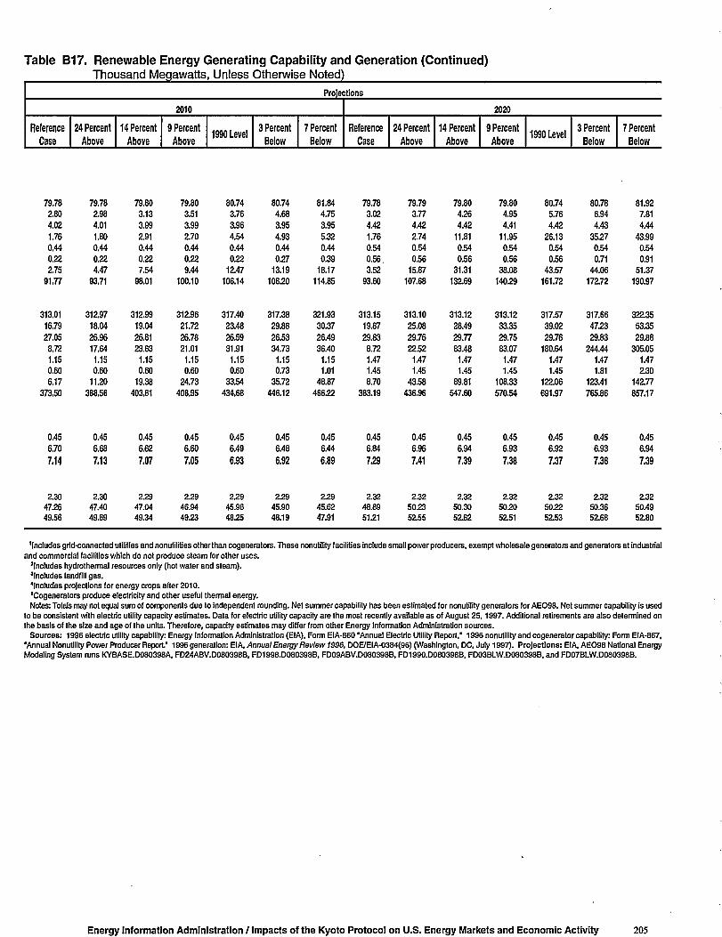
Table B17. Renewable Energy Generating Capability and Generation (Continued)Thousand Megawatts, Unless Otherwise Noted)
Projections
2010
ReferenceCase
24 PercentAbove
14 PercentAbove
9 PercentAbove
1990 Level3 Percent
Below7 Percent
Below
2020
ReferenceCase
24 PercentAbove
14 PercentAbove
9 PercentAbove
1990 Level3 Percent
Below7 Percent
Below
79.78
2.80
4.02
1.76
0.44
0.22
2.75
91.77
313.01
16.79
27,05
8.72
1.15
0.60
6.17
373.50
0.45
6.70
7.14
2.3047.26
49.56
79.78
2.98
4.01
1.80
0.44
0.22
4.47
93.71
312.97
18.04
26.96
17.64
1.15
0.60
11.20
388.56
0.45
6.68
7.13
2.3047.40
49.69
79.80
3.13
3.99
2.91
0.44
0.22
7.54
98.01
312.99
19.04
26.81
23.63
1.15
0.60
19.38
403.61
0.45
6.62
7.07
2.2947.04
49.34
79.80
3.51
3.99
2.70
0.44
0.22
9.44
100.10
312.96
21.72
26.78
21.01
1.15
0.60
24.73
408.95
0.45
6.60
7.05
2.29
46.94
49.23
80.74
3.76
3.96
4.54
0.44
05212.47
106.14
317.40
23.48
26.59
31.91
1.15
0.60
33.54
434.68
0.45
6.49
6.93
2.29
45.96
48.25
80.74
4.68
3.95
4.93
0.44
0.27
13.19
108.20
317.38
29.88
26.53
34.73
1.15
0.73
35.72
446.12
0.45
6.48
6.92
2.29
45.90
48.19
81.84
4.75
3.95
5.32
0.44
0.39
18.17
114.85
321.93
30.37
26.49
36.40
1.15
1.01
48.87
46622
0.45
6.44
6.89
25945.62
47.91
79.78
3.02
4.42
1.76
0.54
0.56.
3.52
93.60
313.15
19.87
29.83
8.72
1.47
1.45
8.70
383.19
0.45
6.84
7.29
2.32
48.89
5151
79.79
3.77
4.42
2.74
0.54
0.56
15.87
107.68
313.10
25.08
29.76
22.52
1.47
1.45
43.58
436.96
0.45
6.96
7.41
2.32505352.55
79.80
4.26
4.42
11.81
0.54
0.56
31.31
132.69
313.12
28.49
29.77
83.48
1.47
1.45
89.81
547.60
0.45
6.94
7.39
2.3250.3052.62
79.80
4.95
4.41
11.95
0.54
0.56
38.08
14059
313.12
33.35
29.75
83.07
1.47
1.45
108.33
570.54
0.45
6.93
7.38
£3250505Z51
80.74
5.76
4.42
26.13
0.54
0.56
43.57
161.72
317.57
39.02
29.76
180.64
1.47
1.45
122.06
691.97
0.45
6.92
7.37
2.32505252.53
80.78
6.94
4.43
35.27
0.54
0.71
44.06
172.72
317.66
47.23
29.83
244.44
1.47
1.81
123.41
765.86
0.45
6.93
7.38
2.3250.36
52.68
81.92
7.81
4.44
43.99
0.54
0.91
51.37
190.97
322.35
53.35
29.88
305.05
1.47
2.30
142.77
857.17
0.45
6.94
7.39
2.3250.49
52.80
'Includes grid-connected utilities and nonutilitles other than cogenerators. These nonutility facilities include small powerproducers, exempt wholesale generators and generators at industrialand commercial facilities which do not produce steam for other uses.
'Includes hydrothermal resources only (hot water and steam).'Includes landfill gas.'Includes projections for energy crops after 2010.'Cogenerators produce electricity and other useful thermal energy.Notes: Totals may not equal sum of components due to independent rounding. Net summer capability has been estimated for nonutility generators for AEO98. Net summer capability is used
to be consistent with electric utility capacity estimates. Data for electric utility capacity are the most recently available as of August 25,1997. Additional retirements are also determined onthe basis of the size and age of the units. Therefore, capacity estimates may differ from other Energy Information Administration sources.
Sources: 1996 electric utility capability: Energy Information Administration (EIA), Form EIA-860 'Annual Electric Utility Report,' 1996 nonutility and cogenerator capability: Form EIA-867,"Annual Nonutility Pov/er Producer Report." 1996 generation: EIA, Annual Energy Review 1996, DOE/EIA-0384(96) (Washington, DC, July 1997). Projections: EIA, AEO98 National EnergyModeling System runs KYBASE.D080398A, FD24ABV.D080398B, FD1998.D080398B, FD09ABV.D080398B, FD1990.D080398B, FD03BLW.D080398B, and FD07BLW.D080398B.
Energy Information Administration / Impacts of the Kyoto Protocol on U.S. Energy Markets and Economic Activity 205
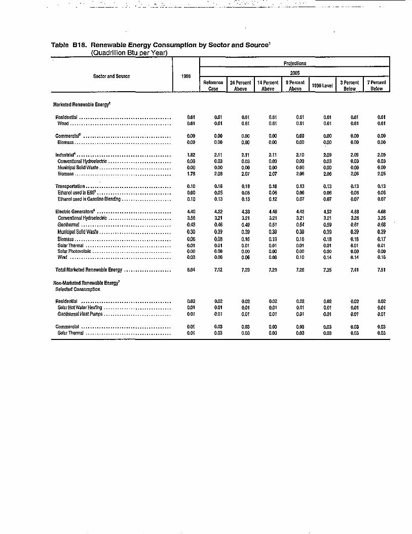
Table B18. Renewable Energy Consumption by Sector and Source1
(Quadrillion Btu per Year)
Sector and Source 1996
Projections
2005
Reference
Case
24 Percent
Above
14 Percent
Above
9 Percent
Above1990 Level
3 Percent
Below
7 Percent
Below
Marketed Renewable Energy2
Residential ,Wood ,
Commercial3
Biomass
Industrial4
Conventional HydroelectricMunicipal Solid WasteBiomass
Transportation ,Ethanol used in E855
Ethanol used in Gasoline Blending .
Electric Generators8 ,Conventional HydroelectricGeothermalMunicipal Solid WasteBiomass ,Solar Thermal ,Solar PhotovoltaicWind
Total Marketed Renewable Energy ,
Non-Marketed Renewable Energy7
Selected Consumption
Residential ,
Solar Hot Water Heating
Geothermal Heat Pumps
Commercial
Solar Thermal
0.61
0.61
0.00
0.00
1.82
0.03
0.00
1.78
0.10
0.00
0.10
4.40
3.56
0.43
0.300.06
0.010.000.03
0.61
0.61
0.00
0.00
2.11
0.03
0.00
2.08
0.18
0.05
0.13
4.22
3.21
0.46
0.39
0.08
0.010.000.06
0.61
0.61
0.00
0.00
2.11
0.03
0.00
2.07
0.18
0.05
0.13
4.33
3.21
0.49
0.39
0.160.010.000.06
0.61
0.61
0.00
0.00
2.11
0.03
0.00
2.07
0.18
0.06
0.12
4.40
3.21
0.51
0.390.19
0.010.000.08
0.61
0.61
0.00
0.00
2.10
0.03
0.00
2.06
0.13
0.06
0.07
4.42
3.21
0.54
0.390.16
0.010.000.10
0.61
0.61
0.00
0.00
2.09
0.03
0.00
2.06
0.13
0.06
0.07
4.52
3.21
0.59
0.39
0.18
0.010.000.14
0.61
0.61
0.00
0.00
2.09
0.03
0.00
2.06
0.13
0.06
0.07
4.58
3.26
0.61
0.390.180.010.000.14
0.61
0.61
0.00
0.00
2.09
0.03
0.00
2.05
0.13
0.06
0.07
4.68
3.26
0.68
0.390.170.010.000.16
6.94 7.12 7.23 7.29 7.26 7.35 7.41 7.51
0.02
0.01
0.01
0.01
0.01
0.02
0.01
0.01
0.03
0.03
0.02
0.01
0.01
0.03
0.03
0.02
0.01
0.01
0.03
0.03
0.02
0.01
0.01
0.03
0.03
0.02
0.01
0.01
0.03
0.03
0.02
0.01
0.01
0.03
0.03
0.02
0.01
0.01
0.03
0.03

Table B18. Renewable Energy Consumption by Sector and Source1 (Continued)(Quadrillion Btu per Year)
Projections
2010
ReferenceCase
24 PercentAbove
14 PercentAbove
9 PercentAbove
1990 Level3 Percent
Below7 Percent
Below
2020
ReferenceCase
24 PercentAbove
14 PercentAbove
9 PercentAbove
1990 Level3 Percent
Below7 Percent
Below
0.61
0.61
0.00
0.00
2.25
0.03
0.00
2.21
0.23
0.09
0,13
4.30
3.22
0.49
0.43
0.03
0,01
0,010.06
0.61
0.61
0.00
0.00
2.25
0.03
0.00
2.21
0.19
0.09
0.09
4.47
3.22
0.53
0.43
0.16
0.01
0.01
0,12
0.62
0.62
0.00
0.00
2.24
0.03
0.00
2.20
0.23
0.10
0.13
4.63
3.22
0.56
0.43
0.21
0.01
0,0f
0.20
0.62
0.62
0.00
0.00
2.23
0.03
0.00
2.20
0.22
0.10
0.12
4.75
3.22
0.64
0.43
0.19
0.01
0.01
0.25
0.63
0.63
0.00
0.00
2.19
0.03
0.00
2.15
0.23
0.09
0.13
5.05
3.26
0.72
0.43
0.28
0.01
0.010.34
0.63
0.63
0.00
0.00
2.18
0.03
0.00
2.15
0.39
0.09
0.30
5.31
3.26
0.93
0.42
0.31
0.01
0.01
0.37
0.63
0.63
0.00
0.00
2.17
0.03
0.00
2.13
0.53
0.09
0.45
5.53
3.31
0.95
0.42
0.32
0.01
0.01
0.50
0.62
0.62
0.00
0.00
2.35
0.03
0.00
2.31
0.31
0.13
0.18
4.47
3.22
0.59
0.48
0.08
0.00
0.01
0.09
0.63
0.63
0.00
0.00
2.39
0.03
0.00
2.35
0.29
0.14
0.15
5.11
3.22
0.75
0.48
0.20
0.00
0.01
0.45
0.64
0.64
0.00
0.00
2.39
0.03
0.00
2.36
0.38
0.14
0.24
6.23
3.22
0.85
0.48
0.74
0.00
0.01
0.92
0.64
0.64
0.00
0.00
2.39
0.03
0.00
2.35
0.40
0.14
056
6.58
3.22
1.01
0.48
0.74
0.00
0.01
1.11
0.65
0.65
0.00
0.00
2.39
0.03
0.00
2.35
0.57
0.13
0.44
7.85
3.26
1530.48
1.61
0.00
0.01
1.25
0.66
0.66
0.00
0.00
2.39
0.03
0.00
2.36
0.69
0.13
0.56
8.71
3.27
1.50
0.48
2.18
0.00
0.02
1.27
0.67
0.67
0.00
0.00
2.40
0.03
0.00
2.36
0.69
0.13
0.56
9.72
3.31
1.71
0.48
2.72
0.00
0.02
1.47
7.39 7.52 7.71 7.83 8.10 8.52 8.87 7.75 8.42 9.65 10.01 11.47 12.45 13.47
0,03
0,01
0.02
0.03
0.03
0.03
0.01
0.02
0.03
0.03
0.03
0.01
0.02
0.03
0.03
0.03
0.01
0.02
0.03
0.03
0.03
0.01
0.02
0.03
0.03
0.03
0.01
0.02
0.03
0.03
0.03
0.01
0.02
0.03
0.03
0.05
0.01
0.04
0.04
0.04
0.05
0.01
0.04
0.04
0.04
0.05
0.01
0.04
0.04
0.04
0.05
0.01
0.04
0.04
0.04
0.05
0.01
0.04
0.04
0.04
0.06
0.01
0.05
0.04
0.04
0.06
0.010.05
0.04
0.04
'Actual heat rates used to determine fuel consumption for all renewable fuels except hydropower, solar, and wind. Consumption at hydroelectric, solar, and wind facilities determined byusing the fossil fuel equivalent of 10,280 Btu per kilowatthour.
'Includes nonelectric renewable energy groups for which the energy source is bought and sold in the marketplace, although all transactions may not necessarily be marketed, and marketedrenewable energy inputs for electricity entering the marketplace on the electric power grid. Excludes electricity imports; see Table B8.
'Value Is less than 0.005 quadrillion Btu per year and rounds to zero.'Includes all electricity production by industrial and other cogenerators for the grid and for own use.'Excludes motor gasoline component of E85.'Includes renev/able energy delivered to the grid from electric utilities and nonutilities. Renewable energy used in generating electricity for own use is included in the individual sectoral
electricity energy consumption values.'Includes selected renev/able energy consumption data for which the energy is not bought or sold, either directly or indirectly as an input to marketed energy. The Energy Information
Administration does not estimate or project total consumption of nonmarketed renewable energy.Btu = British thermal unit.Notes: Totals may not equal sum of components due to independent rounding.Sources: 1996 electric generators: Energy Information Administration (EIA), Form EIA-860, "Annual Electric Utility Report" and EIA, Form EIA-867, "Annual Nonutility Power Producer
Report." 1996 ethanol: EIA, Petroleum Supply Annual 1996, DOE/EIA-O340(96/1) (Washington, DC, June 1997). Other 1996: EIA, Office of Integrated Analysis and Forecasting. Projections:EIA, AEO98 National Energy Modeling System runs KYBASE.D080398A, FD24ABV.D080398B, FD1998.D080398B, FD09ABV.D080398B, FD1990.D080398B, FD03BLW.D080398B, andFD07BLW.D080398B.
Energy Information Administration / I t >acts of the 1. oto Protocol on U.S. Ener< Markets and Economic Activit 207

Table B19. Carbon Emissions by Sector and Source(Million Metric Tons per Year)
Sector and Source 1996
Projections
2005
Reference
Case
24 Percent
Above
14 Percent
Above
9 Percent
Above1990 Level
3 Percent
Below
7 Percent
Below
Residential
Petroleum 27.3
Natural Gas 77.4
Coal 1.4
Electricity 179.9
Total .- 286.0
Commercial
Petroleum 15.3
Natural Gas 47.4
Coal 2.1
Electricity 164.8
Total 229.6
Industrial'
Petroleum 104.8
Natural Gas2 142.8
Coal 59.3
Electricity 169.2Total 476.1
TransportationPetroleum3 457.9
NaturalGas4 10.5
Other5 0.0
Electricity 2.8
Total3 4715
Total Carbon Emissions6
Petroleum3 605.3
NaturalGas 278.1
Coal 62.8
Other5 0.0
Electricity 516.7
Total3 1462.9
Electric Generators7
Petroleum 15.5
Natural Gas 40.3
Coal 460.9
Total 516.7
Total Carbon Emissions9
Petroleum3 620.8
NaturalGas 318.4
Coal 523.7
Other5 0.0
Total3 1462.9
Carbon Emissions(tons per person) 5.5
24.079.6
1.4
217.6
322.6
12.6
52.3
2.3196.4
263.6
110.5
155.9
66.0203.4535.7
549.4
14.0
1.4 .
4.2569.0
696.4
301.9
69.7
1.4621.5
1690.9
8.877.8
534.9
621.5
705.2
379.7
604.6
1.41690.9
24.0
79.4
1.4212.3
317.1
12.6
52.2
2.3191.7
258.8
110.1
156.0
65.5198.4530.0
548.7
14.5
1.54.1
568.7
695.4
302.1
69.2
1.5606.4
1674.6
8.482.5
515.5
606.4
703.8
384.6
584.7
1.51674.6
23.477.1
1.2
199.3
301.0
12.2
50.5
2.3179.5
244.5
109.7
156.5
58.2188.351Z8
545.6
14.4
1.53.9
565.4
691.0
298.6
61.7
1.5571.0
1623.7
7.786.3
476.9
571.0
698.7
384.9
538.7
1.51623.7
23.1
75.6
1.2187.5
287.3
12.0
49.3
2.2168.0
231.5
108.2
158.0
54.0178.0498.2
543.0
14.3
1.53.7
562.5
686.3
297.2
57.4
1.5537.1
1579.5
7.392.3
437.5
537.1
693.6
389.4
494.9
1.51579.5
23.0
75.1
1.1181.0
280.2
11.9
48.8
2.2161.4
224.4
107.5
158.3
52.8171.5490.0
541.2
14.4
1.53.6
560.6
683.6
296.5
56.1
•1.5
517.5
1555.2
7.096.3
414.3
517.5
690.5
392.8
470.4
1.51555.2
22.9
74.8
1.1178.6
277.4
11.9
48.6
2.2159.6
222.2
107.0
158.652.2
169.2487.0
539.9
14.5
1.53.6
559.5
681.6
• 296.5
55.5
1.5511.0
1546.1
6.5101.8
402.7
511.0
688.1
398.3
458.2
1.51546.1
22.8
74.3
1.1174.4
272.5
11.8
48.1
2.2155.5
217.5
106.6
158.451.6
164.9481.6
538.5
14.5
1.53.5
557.9
679.7
295.2
54.8
1.5498.3
1529.6
7.2102.3
388.9
498.3
686.9
397.5
443.7
1.51529.6
5.9 5.8 5.7 5.5 5.4 5.4 5.3

Table B19. Carbon Emissions by Sector and Source (Continued)(Million Metric Tons per Year)
Projections
2010
ReferenceCase
23,382,31,4
230,3337.3
12,554,62.5
207,6277.2
115,7162.467.1
214.3559.4
592.916,22.55.1
616.7
744.3315.570,92,5
657.41790.6
7.599,5
550.4657.4
751,8415,0621.3
2.51790.6
6.0
24 PercentAbove
22.578.31.2
198.8300.7
12.051.72.3
178,0244.1
113.7163,156.4
185.6518.7
580.916.42.64.6
604.5
729.1309.559,82,6
567.01667.9
6.2114.2446.6567.0
735.3423.7506.4
2.61667.9
5.6
14 PercentAbove
21.774.21.0
164.7261.7
11.548.42.1
145.8207.9
113.1163.750,1
154.0480.9
561.7
16.5
2.53.8
584.5
708.1
302,8
53.3
2.5468.3
1535.0
5.1136,5326.7468.3
713,2439.3379.9
2.51535.0
5.1
9 PercentAbove
21.472.01.0
143.9238.3
11.346.42.1
126,3186.1
113.5
164.148.4
135.6461.5
552.617.12.53.4
575.6
698.7299.751.42.5
409.11461.5
5.0156.4247.7409.1
703.8456.1299.1
2.51461.5
4.9
'tQOn 1 airaliyyu Level
20.568.00.9
117.9207.3
10.742.11.9
101.1155.7
1105162.743.9
110.1427.3
527.6
16.8
2.42.8
549.6
669.3289.746.72.4
331.91340.0
5.1174.5152.3
331.9
674.4464.2199.1
2.41340.0
4.5
3 PercentBelow
20.066.80.9
111.1198.7
10.440.51.8
94.4147.1
108.6
162.542.7
104.2418.0
514.4
16.8
2.32.6
536.2
653.3
286.6
45.42.3
312.41300.0
6.9179.3
126.1
312.4
660.3
465.9
171.5
2.31300.0
4.3
7 PercentBelow
19.564.90.9
101.9187.1
10.038.11.7
85.6135.3
1095158.241.495.2
403.9
495.7
16.6
2.32.4
517.1
634.3277.843.92.3
285.01243.4
7.9182.3
94.8
285.0
642.2460.2138.7
2.31243.4
45
2020
ReferenceCase
22.286.11.4
265.7375.4
12.156.62.6
227.3298.6
120.7
167.466.9
226.6581.6
644.1
19.0
3.86.4
673.2
799.1
329.0
70.83.8
726.0
1928.7
5.9138.8
581.3
726.0
805.0
467.8
652.1
3.81928.7
6.0
24 PercentAbove
21.078.41.1
190.3290.8
11.451.12.3
160.42255
121.9165.653.6
163.8504.9
618.8
19.7
3.84.8
647.1
773.1
314.8
57.0
3.8519.4
1668.0
3.8179.8
335.8
519.4
776.9494.6392.8
3.81668.0
55
14 PercentAbove
20.875.11.0
149.9246.8
11.2
48.6
2.2125.3187.4
124.8162.651.8
128.5467.7
606.6
20.2
3.83.8
634.3
763.5
306.5
55.0
3.8407.5
15365
4.6201.0
201.9
407.5
768.1
507.5
256.9
3.815365
4.7
9 PercentAbove
20.673.41.0
129.5224.4
11.147.12.1
107.8168.1
127.0
160.750.4
110.8449.0
598.9
20.3
3.73.3
626.3
757.6
301.6
53.6
3.7351.3
1467.8
9.3215.0
127.0
351.3
767.0516.5180.5
3.71467.8
4.5
1OOft I awali yyu LcVci
19.870.40.9
99.2190.3
10.744.42.0
81.7138.7
1255160.546.184.7
416.8
574.6
20.1
3.62.5
600.8
730.6
295.4
49.0
3.6268.0
1346.7
13.8218.435.9
268.0
744.4513.8
84.93.6
1346.7
45
3 PercentBelow
19.369.20.9
91.1180.5
10.443.11.8
74.4129.8
123.6159.743.777.7
404.7
562.5
19.8
3.52.3
5885
'715.9
291.8
46.53.5
245.51303.3
10.7215.6
19.2245.5
726.6507.465.73.5
1303.3
4.0
7 PercentBelow
f8.667.40.9
81.3168.1
10.0
40.9
1.765.8
118.3
120.2
161.641.169.5
392.4
547.2
19.3
3.42.0
571.9
696.0
289.1
43.6
3.4218.6
1250.8
6.1206.1
6.4218.6
702.1495.3
50.03.4
1250.8
3.9
'Includes consumption by cogenerators.'Includes lease and plant fuel.Th i s includes intemational bunker fuels which, by convention, are excluded from the intemational accounting of carbon emissions. In the years from 1989 through 1996, intemational bunker
fuels account for 22 to 24 million metric tons of carbon annually.'Includes pipeline fuel natural gas and compressed natural gas used as vehicle fuel.'Includes methanol and liquid hydrogen."Measured for delivered energy consumption.'Includes all electric power generators except cogenerators, v/hich produce electricity and other useful thermal energy.•Measured for total energy consumption, with emissions for electric power generators distributed to the primary fuels.
Note; Totals may not equal sum of components due to independent rounding.Sources: Carbon coefficients from Energy Information Administration, (EIA) Emissions of Greenhouse Gasesin the United Slates 1996, DOE/ElA-0573(96) (Washington, DC, October 1997).
1996 consumption estimates based on: EIA, Short Term Energy Outlook, August 1997, Online. http://www.eia.doe.gov/emeu/st.eo/pub/upd/aug97/index.html (August 21,1997). Prelections:EIA, AEO98 National Energy Modeling System run KYBASE.D080398A, FD24ABV.D080398B, FD1998.D080398B, FD09ABV.D080398B, FD1990.D080398B, FD03BLW.D080398B, andFD07BLW.D080398B.
Energy Information Administration / Impacts of the Kyoto Protocol on U.S. Energy Markets and Economic Activity 209

Table B20. Macroeconomic Indicators(Billion 1992 Chain-Weighted Dollars, Unless
Indicators 1996
Otherwise Noted)
Projections
2005
Reference
Case
24 Percent
Above
14 Percent
Above
9 Percent
Above1990 Level
3 Percent
Below
7 Percent
Below
GDP Chain-Type Price Index
(1992=1.000) 1.102
Real Gross Domestic Product 6928
Real Consumption 4714
Real Investment 1069
Real Government Spending 1258'
Real Exports 857
Real Imports 971
Real Disposable Personal Income 5077
M Utility Bond Rate (percent) 7.57
Real Yield on Government 10 Year Bonds
(percent) 4.99
Energy Intensity
(thousand Btu per 1992 dollar of GDP)
Delivered Energy 10.14
Total Energy 13.54
ConsumerPricelndex(1982-84=1.00) 1.57
Unemployment Rate (percent) 5.38
Unit Sales of Ught-Duty Vehicles (million) 15.10
Millions of People
Population with Armed Forces Overseas 266.1
Population (aged 16 and over) 204.2
LaborForce 133.9
1.380 1.382 1.393 1.401 1.404 1.406 1.408
8525
5738
1513
1386
1753
1859
6206
7.14
8520
5735
1509
1386
1753
1857
6205
7.17
8495
5730
1488
1385
1749
1854
6218
7.39
8474
5724
1473
1384
1746
1853
6224
7.55
8464
5721
1464
1383
1745
1851
6225
7.62
8462
5722
1462
1383
1744
1852
6230
7.66
8454
5719
1457
1383
1744
1852
6228
7.70
3.78 3.79 3.89 3.97 4.00 4.02 4.04
9.36
12.42
2.04
5.70
15.69
287.1
223.8
149.7
9.36
12.37
2.04
5.72
15.60
287.1223.8
149.7
9.26
12.17
2.06
5.80
15.19
287.1
223.8
149.7
9.18
12.00
2.07
5.87
14.91
287.1223.8
149.6
9.15
11.94
2.08
5.91
14.79
287.1223.8
149.6
9.13
11.92
2.08
5.91
14.73
287.1
223.8
149.6
9.11
11.86
2.09
5.94
14.64
287.1223.8
149.6

Table B20. Macroeconomic Indicators (Continued)(Billion 1992 Chain-Weighted Dollars, Unless Otherwise Noted)
Projections
2010
Reference
Case
24 Percent
Above
14 Percent
Above
9 Percent
Above1990 Level
3 Percent
Below
7 Percent
Below
2020
Reference
Case
24 Percent
Above
14 Percent
Above
9 Percent
Above1990 Level
3 Percent
Below
7 Percent
Below
1.606 1.628 1.645 1.655 1.679 1.688 1.701 2.281 2.303 2.308 2.317 2.327 2.333 2.337
9429
6347
1745
1499
2337
2519
6891
7.31
9333
6292
1714
1486
2318
2509
6835
7.42
9268
6258
1716
1473
2296
2520
6794
7.38
9241
6248
1719
1468
2283 •
2532
6783
7.36
9137
6207
1692
1454
2248
2541
6752
7.43
9102
6198
1682
1450
2232
2550
6751
7.47
9032
6160
1662
1442
2215
2548
6719
7.66
10865
7599
2100
1636
3333
4123
8192
8.50
10815
7573
2101
1622
3316
4153
8144
8.37
10808
7582
2099
1623
3296
4179
8151
8.33
10796
7583
2098
1622
3282
4195
8153
8.34
10799
7615
2101
1623
3252
4247
8188
8.30
10793
7631
2100
1622
3233
4274
8209
8.31
10782
7636
2095
1621
3218
4290
8214
8.27
3,58 3.55 3.64 3.71- 3.74 3.81 3.95 4.10 4.15 4.17 4.20 459 4.33 4.33
8.98
11.80
2.43
5.58
16.57
298.9
235.4
156.5
8.82
11.42
2.46
6.06
16.06
298.9
235.4
156.0
8.63
11.00
2.49
6.38
15.96
298.9235.4155.6
8.54
10.78
2.51
6.51
15.96
298.9
235.4
155.4
8.30
10.43
2.56
7.01
15.61
293.9
235.4
154.9
8.21
- 10.33
2.57
7.16
15.48
298.9
235.4
154.7
8.08
10.16
2.60
7.49
15.16
298.9235.4154.4
8.31
10.78
3.56
5.78
17.04
323.5
255.6
162.2
7.99
10.05
3.61
5.90
16.69
323.5.255.6162.0
7.87
9.78
3.62
5.91
16.70
323.5255.6161.9
7.79
9.62
3.63
5.94
16.66
323.5255.6161.9
7.59
9.35
3.65
5.86
16.69
323.5255.6161.9
7.49
9.27
3.66
5.84
16.68
323.5255.6161.8
7.36
9.17
3.68
5.85
16.51
323.5255.6161.8
GDP = Gross domestic product.
Btu = British thermal unit.
Source: Simulations of the Data Resources, Inc. (DRI) Model of the U.S. Economy.
Energy Information Administration / Impacts of the Kyoto Protocol on U.S. Energy Markets and Economic Activity 211

This page is intentionally left blank.

Appendix C
Summary Comparison of Analyses

This page Is intentionally left blank.

Table C1 • Summary of the WEFA Analysis
Parameter 1996
ReferenceCase in
2010
1990-7%Case in
2010
ReferenceCase in
2020
1990-7%Case in
2020Carbon Price (1996 Dollars per Metric Ton)Gross Domestic Product (Billion 1992 Chain-Weighted Dollars). . . .Total Carbon Emissions (Million Metric Tons)
Per Capita Carbon Emissions (Metric Tons per Person)
Real Disposable Personal Income (Billion 1992 Dollars)
Real Investment (Billion 1992 Dollars)*
Real Consumption (Billion 1992 Dollars)
Light-Duty Vehicle Sales (Millions)
Primary Energy Intensity (Thousand Btu per 1992 Dollar of GDP). . .
Delivered Energy Intensity (Thousand Btu per 1992 Dollar of GDP). .
World Oil Price (Refiners Acquisition Price, 1996 Dollars per Barrel) .
Natural Gas Wellhead Price (1996 Dollars per Thousand Cubic Feet).
Minemouth Coal Price (1996 Dollars per Short Ton)
Carbon Intensity (Metric Tons per Thousand 1992 Dollars of GDP) . .
Delivered Energy Prices (1996 Dollars)
Coal (Dollars per Million Btu to Utilities)
Natural Gas (Dollars per Thousand Cubic Feet)
Distillate (Dollars per Gallon)
Motor Gasoline (Dollars per Gallon)
Electricity (Cents per Kilowatthour)
Total Primary Energy Consumption (Quadrillion Btu)
Fossil Fuel Consumption (Quadrillion Btu)
Natural Gas
CoafPetroleumTotal
Total End-Use Carbon Emissions (Million Metric Tons)
Buildings (Residential/Commercial)"Industrial0
TransportationElectricity
Energy Consumption for Electricity Generation (Quadrillion Btu)CoalNatural GasNuclearRenewables
Petroleum
Electricity Sales (Quadrillion Btu)
NA6,9281,463
5.5
5,0771,067
4,714
15.1
13.57
10.16
20.482.24
18.50
0.217
1.29
4.25
1.09
1.23
6.9
94.0
22.6
20.936.079.51,463
170.9
306.9
468.4
516.7
18.36
3.04
7.20
4.47
0.75
10.57
NA9,3141,700
5.7
6,9421,527
6,303
16.7
11.08
8.24
19.77
2.09
16.43
0.183
1.19
3.92
1.21
1.24
5.9103.2
29.9
22.840.793.41,700
—
470.3
564.0665.7
20.35
8.91
6.02
3.79
0.6913.24
2659,0131,247
4.2
6,8401,468
6,152
16.2
9.30
7.20
17.58
2.19
12.82
0.138
7.71
7.61
1.89
1.83
9.8
83.9
30.1
8.435.373.91,247
—
369.1
507.6
370.8
7.10
12.64
6.02
4.00
0.52
11.04
NA11,4781,953
6.0
8,6711,923
7,705
18.3
9.98
7.45
21.38
2.24
15.05
0.170
1.11
3.79
1.23
1.30
5.6
114.5
36.4
25.845.2107.41,952
—
501.1
642.5
809.0
23.32
13.62
3.25
3.81
0.6315.63
36011,2451,231
3.8
8,5961,894
7,651
18.3
7.50
6.05
17.57
2.46
11.44
0.109
10.06
8.95
2.14
2.08
10.3
84.4
37.0
2-737.276.91,231
—
359.6
550.1
321.9
1.64
19.26
3.25
4.22
0.05
12.06
^Calculated as the sum of residential investment plus nonresidential fixed investment.Excludes emissions related to electricity generation.
°The WEFA projection provides an "other category" which combines direct emissions from the Buildings and Industrial sectors.Sources: 1996: Energy Information Administration, Annual Energy Outlook 1998, DOE/EIA-0383(98) (Washington, DC, December 1997). 2010
and 2020: WEFA, Inc., Global Warming: The High Cost of the Kyoto Protocol, National and State Impacts (1998). The WEFA report did not coveranalyses of alternative carbon emissions targets because they did not believe that a workable comprehensive international trading system could beimplemented in time and that developing countries would not participate in the clean development mechanism.
Energy Information Administration / Impacts of the Kyoto Protocol on U.S. Energy Markets and Economic Activity 215
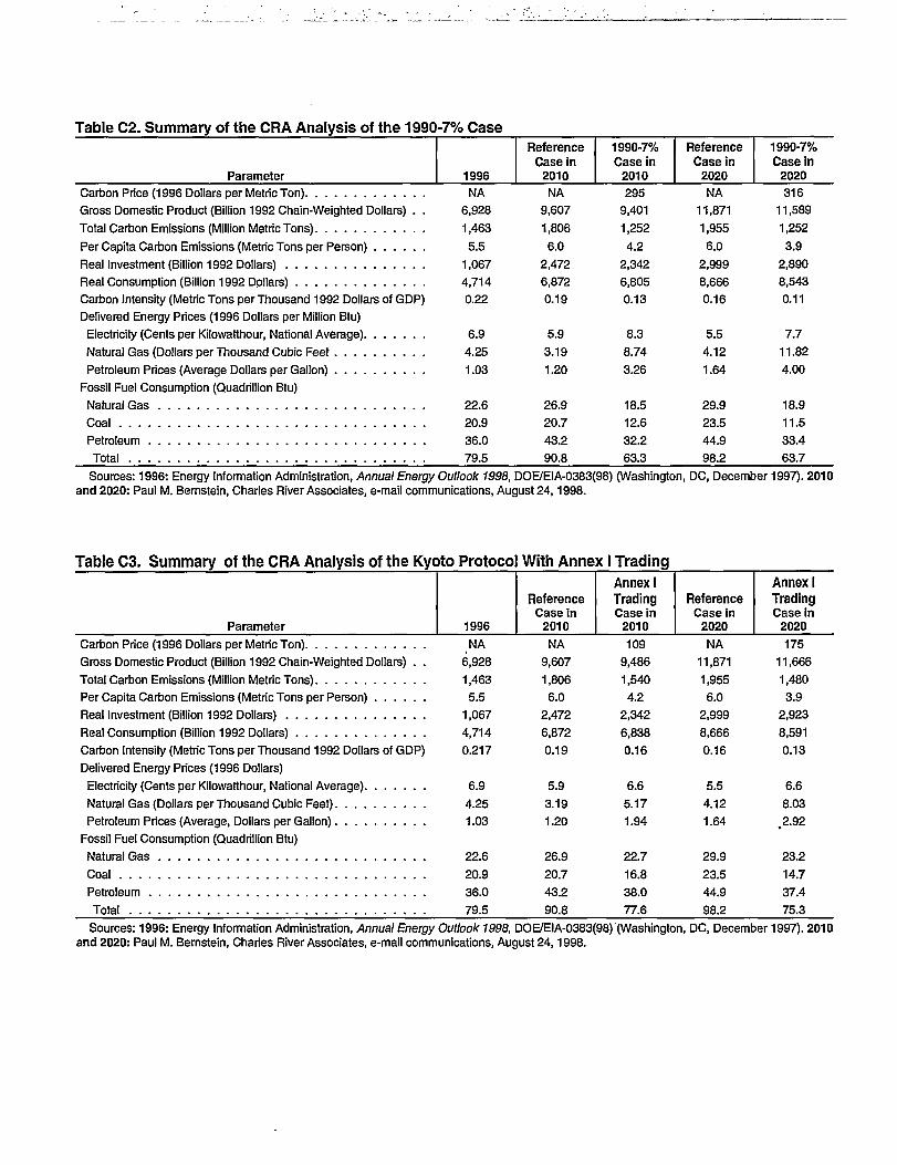
Table C2. Summary of the CRA Analysis of the 1990-7% Case
Parameter 1996
ReferenceCase in
2010
1990-7%Case in
2010
ReferenceCase in
2020
1990-7%Case in
2020Carbon Price (1996 Dollars per Metric Ton)
Gross Domestic Product (Billion 1992 Chain-Weighted Dollars) . .
Total Carbon Emissions (Million Metric Tons)
Per Capita Carbon Emissions (Metric Tons per Person)
Real Investment (Billion 1992 Dollars)
Real Consumption (Billion 1992 Dollars)
Carbon Intensity (Metric Tons per Thousand 1992 Dollars of GDP)
Delivered Energy Prices (1996 Dollars per Million Btu)
Electricity (Cents per Kilowatthour, National Average)
Natural Gas (Dollars per Thousand Cubic Feet
Petroleum Prices (Average Dollars per Gallon)
Fossil Fuel Consumption (Quadrillion Btu)
Natural GasCoalPetroleum
Total
NA6,928
1,463
5.5
1,067
4,714
0.22
6.9
4.25
1.03
22.6
20.9
36.0
79.5
NA9,607
1,806
6.0
2,472
6,872
0.19
5.9
3.19
1.20
26.9
20.7
43.2
90.8
2959,401
1,252
4.2
2,342
6,805
0.13
8.3
8.74
3.26
18.5
12.6
32.2
63.3
NA11,871
1,955
6.0
2,999
8,666
0.16
5.5
4.12
1.64
29.9
23.5
44.9
98.2
31611,589
1,252
3.92,890
8,543
0.11
7.711.82
4.00
18.9
11.5
33.4
63.7
Sources: 1996: Energy Information Administration, Annual Energy Outlook 1998, DOE/EIA-0383(98) (Washington, DC, December 1997). 2010and 2020: Paul M. Bernstein, Charles River Associates, e-mail communications, August 24,1998.
Table C3. Summary of the CRA Analysis of the Kyoto Protocol With Annex I Trading
Parameter 1996
ReferenceCase in
2010
Annex ITradingCase in
2010
ReferenceCase in
2020
Annex ITradingCase in
2020
Carbon Price (1996 Dollars per Metric Ton)
Gross Domestic Product (Billion 1992 Chain-Weighted Dollars) . .
Total Carbon Emissions (Million Metric Tons)
Per Capita Carbon Emissions (Metric Tons per Person)
Real Investment (Billion 1992 Dollars)
Real Consumption (Billion 1992 Dollars)
Carbon Intensity (Metric Tons per Thousand 1992 Dollars of GDP)
Delivered Energy Prices (1996 Dollars)
Electricity (Cents per Kilowatthour, National Average)
Natural Gas (Dollars per Thousand Cubic Feet)
Petroleum Prices (Average, Dollars per Gallon)
Fossil Fuel Consumption (Quadrillion Btu)
Natural GasCoalPetroleum
Total
NA6,928
1,463
5.5
1,067
4,714
0.217
6.9
4.25
1.03
22.6
20.9
36.0
79.5
NA9,607
1,806
6.0
2,472
6,872
0.19
5.9
3.19
1.20
26.9
20.7
43.2
90.8
1099,486
1,540
4.2
2,342
6,838
0.16
6.6
5.17
1.94
22.7
16.8
38.0
77.6
NA11,871
1,955
6.0
2,999
8,666
0.16
5.5
4.12
1.64
29.9
23.5
44.9
98.2
17511,666
1,480
3.9
2,923
8,591
0.13
6.6
8.03
2.92
23.2
14.7
37.4
75.3
Sources: 1996: Energy Information Administration, Annual Energy Outlook 1998, DOE/EIA-0383(98) (Washington, DC, December 1997). 2010and 2020: Paul M. Bernstein, Charles River Associates, e-mail communications, August 24,1998.

Table C4. Summary of the EPRI Analysis of the 1990-7% Case
Parameter 1996
ReferenceCase in
2010
1990-7%Case in
2010
ReferenceCase in
2020
1990-7%Case in
2020
Carbon Price (1996 Dollars per Metric Ton)a
Gross Domestic Product (Billion 1992 Chain-Weighted Dollars). . .
Total Carbon Emissions (Million Metric Tons)
Per Capita Carbon Emissions (Metric Tons per Person)
Primary Energy Intensity (Thousand Btu per 1992 Dollar of GDP). .
World Oil Price (Refiners Acquisition Price, 1996 Dollars per Barrel)
Carbon Intensity (Metric Tons per Thousand 1992 Dollars of GDP)
(Calculated)Total Primary Energy Consumption (Quadrillion Btu)
Total Fossil Fuel Consumption (Quadrillion Btu)
NA6,928
1,463
5.513.57
20.48
0.217
94
79.51
0
9,296
1,827
6.110.86
23.56
0.197
101
87.31
280
9,203
1,3054.49.13
20.03
0.142
84
0
11,389
1,947
6.09.48
28.27
0.171
108
94.74
251
11,280
1,3054.07.54
24.74
0.116
85
aAII dollars values were given in 1990 dollars by R. Richels, EPRI. To convert from 1990 to 1992 dollars, a deflator of 1.068 was used. To convertfrom 1990 to 1996 dollars, a deflator of 1.178 was used.
Calculated by dividing total primary energy by value of GDP.Sources: 1996: Energy Information Administration, Annual Energy Outlook 1998, DOE/EIA-0383(98) (Washington, DC, December 1997). 2010
and 2020: R. Richels, EPRI, e-mail communications, July 6,1998.
Table C5. Summary of the EPRI Analysis of the Kyoto Protocol With Annex I Trading
Parameter 1996
ReferenceCase in
2010
Annex ITradingCase in
2010
ReferenceCase in
2020
Annex ITradingCase in
2020Carbon Price (1996 Dollars per Metric Ton)
Gross Domestic Product (Billion 1992 Chain-Weighted Dollars). . .
Total Carbon Emissions (Million Metric Tons)Per Capita Carbon Emissions (Metric Tons per Person)
Primary Energy Intensity (Thousand Btu per 1992 Dollar of GDP)(Calculated)
World Oil Price (Refiners Acquisition Price, 1996 Dollars per Barrel)
Carbon Intensity (Metric Tons per Thousand 1992 Dollars of GDP)(Calculated)Total Primary Energy Consumption (Quadrillion Btu)
Total Fossil Fuel Consumption (Quadrillion Btu)
NA
6,928
1,4635.5
13.57
20.48
0.217
94.0
79.51
0
9,296
1,8276.1
10.86
23.56
0.197
101.0
87.31
114
9,245
1,5355.14
9.73
21.20
0.166
90.0
75.78
0
11,389
1,9476.0
9.48
28.27
0.171
108.0
94.74
188
11,199
1,4834.58
8.13
24.74
0.132
91.0
77.01
Sources: 1996: Energy Information Administration, Annual Energy Outlook 1998, DOE/EIA-0383(98) (Washington, DC, December 1997). 2010and 2020: R. Richels, EPRI, e-mail communications, July 6,1998.
Energy Information Administration / Impacts of the Kyoto Protocol on U.S. Energy Markets and Economic Activity 217

Table C6. Summary of the PNNL Analysis of the 1990-7% Case
Parameter 1996
ReferenceCase in
2010
1990-7%Case in
2010
ReferenceCase in
2020
1990-7%Case in
2020
Carbon Price (1996 Dollars per Metric Ton)
Gross Domestic Product (Billion 1992 Chain-Weighted Dollars). .
Total Carbon Emissions (Million Metric Tons)
Per Capita Carbon Emissions (Metric Tons per Person)
Primary Energy Intensity (Thousand Btu per 1992 Dollar of GDP).
Carbon Intensity (Metric Tons per Thousand 1992 Dollars of GDP)
Total Primary Energy Consumption (Quadrillion Btu)
Fossil Fuel Consumption (Quadrillion Btu)
Natural Gas
CoalPetroleum
Total
Energy Consumption for Electricity Generation (Quadrillion Btu)
CoalNatural Gas
Nuclear
Renewables
Petroleum
Electricity Sales (Quadrillion Btu)
NA6,928
1,463
5.513.57
0.217
94.0
22.620.9
36.0
79.5
18.4
3.0
7.2
4.5
0.8
10.6
—
9,416
1,853
6.012.5
0.197
117.7
33.3
24.5
44.5
102.3
20.7
5.0
8.8
4.5
0.1
13.1
2219,357a
1,267
4.310.0
0.135
93.9
33.5
5.8
38.0
77.3
3.0
9.3
9.9
4.6
0.1
10.2
—10,875
2,035
6.111.6
0.187
125.7
38.4
26.6
47.9
112.9
22.2
6.8
5.7
4.5
0.2
13.6
28610,775
1,267
4.08.7
0.118
93.5
38.5
2.9
38.0
79.4
0.5
11.8
6.7
4.8
0.0
9.8aThe GDP values provided are equal to reference level GDP minus the domestic direct cost of meeting the required commitment level. This direct
cost may be different from the welfare loss to the economy.For nuclear and renewable resources, estimated using 1995 benchmark for nuclear resources and corresponding PNNL generation.
Note: The PNL analysis includes a provision for the abatement costs of non-CO2 gases. Abatement costs for the non-CO2 gases are set such thatthe same percentage reduction per dollar of carbon price for those gases is obtained as for CO2. No credits are included for sinks.
Sources: 1996: Energy Information Administration, Annual Energy Outlook 1998, DOE/EIA-0383(98) (Washington, DC, December 1997). 2010and 2020: Ronald Sands, PNNL, e-mail communication, August 26,1998.
Table C7. Summary of the PNNL Analysis of the Kyoto Protocol With Annex I Trading
Parameter 1996
ReferenceCase in
2010
Annex ITradingCase in
2010
ReferenceCase in
2020
Annex ITradingCase in
2020
Carbon Price (1996 Dollars per Metric Ton)
Gross Domestic Product (Billion 1992 Chain-Weighted Dollars). .
Total Carbon Emissions (Million Metric Tons)
Per Capita Carbon Emissions (Metric Tons per Person)
Primary Energy Intensity (Thousand Btu per 1992 Dollar of GDP).
Carbon Intensity (Metric Tons per Thousand 1992 Dollars of GDP)
Total Primary Energy Consumption (Quadrillion Btu)
Fossil Fuel Consumption (Quadrillion Btu)
Natural Gas
CoalPetroleum
Total
Energy Consumption for Electricity Generation (Quadrillion Btu)
CoalNatural Gas
Nuclear
Renewables
Petroleum
Electricity Sales (Quadrillion Btu)
NA6,928
1,463
5.5
13.6
0.217
94.0
22.6
20.9
36.0
79.5
18.43.0
7.2
4.5
0.8
10.6
—9,416
1,853
6.012.5
0.197
117.7
33.3
24.5
44.5
102.3
20.7
5.0
8.84.5
0.1
13.1
1009,381a
1,439
4.910.8
0.153
101.5
33.6
10.4
41.0
85.0
7.38.2
9.6
4.5
0.1
11.0
—10,875
2,035
6.111.6
0.187
' 125.7
38.4
26.6
47.9
112.9
22.2
6.8
5.7
4.5
0.2
13.6
14210,811
1486
4.59.6
0.137
103.3
39.2
8.6
41.8
89.6
5.6
10.5
6.4
4.7
0.1
10.9aThe GDP values provided are equal to reference level GDP minus the domestic direct cost of meeting the required commitment level. This direct
cost may be different from the welfare loss to the economy.For nuclear and renewable resources, estimated using 1995 benchmark for nuclear resources and corresponding PNNL generation.
Note: The PNL analysis includes a provision for the abatement costs of non-CO2 gases. Abatement costs for the non-CO2 gases are set such thatthe same percentage reduction per dollar of carbon price for those gases is obtained as for CO2. No credits are included for sinks.
Sources: 1996: Energy Information Administration, Annual Energy Outlook 1998, DOE/EIA-0383(98) (Washington, DC, December 1997). 2010and 2020: Ronald Sands, PNNL, e-mail communication, August 26,1998.

Table C8. Summary of the El A Analysis of the 1990-7% Case
Parameter 1996
ReferenceCase in
2010
1990-7%Case in
2010
ReferenceCase in
2020
1990-7%Case in
2020
Carbon Price (1996 Dollars per Metric Ton)
Gross Domestic Product (Billion 1992 Chain-Weighted Dollars) . .Total Carbon Emissions (Million Metric Tons). . .
Per Capita Carbon Emissions (Metric Tons per Person)
Real Disposable Personal Income (Billion 1992 Dollars)
Real Investment (Billion 1992 Dollars)
Real Consumption (Billion 1992 Dollars)
Light-Duty Vehicle Sales (Millions) . . . :
Primary Energy Intensity (Thousand Btu per 1992 Dollar of GDP) .Delivered Energy Intensity (Thousand Btu per 1992 Dollar of GDP)World Oil Price (Refiners Acquisition Price, 1996 Dollars per Barrel)Natural Gas Wellhead Price (1996 Dollars per Thousand CubicFeet)
Minemouth Coal Price (1996 Dollars per Short Ton)
Carbon Intensity (Metric Tons per Thousand 1992 Dollars of GDP)
Delivered Energy Prices (1996 Dollars)
Coal (Dollars per Million Btu to Utilities)
Natural Gas (Dollars per Thousand Cubic Feet)
Distillate (Dollars per Gallon)
Motor Gasoline (Dollars per Gallon)
Electricity (Cents per Kilowatthour)Total Primary Energy Consumption (Quadrillion Btu)
Fossil Fuel Consumption (Quadrillion Btu)
Natural Gas
Coal .•PetroleumTotal
Total End-Use Carbon Emissions (Million Metric Tons)a
Buildings (Residential/Commercial)
Industrial
Transportation . . .
Electricity
Energy Consumption for Electricity Generation (Quadrillion Btu)
CoalNatural Gas
Nuclear
Renewables
Petroleum
Electricity Sales (Quadrillion Btu) •
NA6,928
1,463
5.5
5,077
1,067
4,714
15.1
13.57
10.16
20.48
2.24
18.50
0.22
1.29
4.25
1.09
1.23
6.9
94.0
22.6
20.9
36.079.51,463
170.9
306.9
468.4
516.7
18.4
3.0
7.2
4.5
0.8
10.57
NA9,429
1,791
6.0
6,891
1,745
6,347
16.6
11.80
8.98
20.77
2.33
14.29
0.19
1.11
3.87
1.08
1.25
5.9111.2
29.0
24.143.896.91,791
176.6
345.1
611.6
657.4
21.4 •
6.9
6.2
4.3
0.4
• 13.19
348
9,0321,243
4.2
6,719
1,662
6,160
15.2
10.16
8.0817.54
3.03
18.29
0.14
9.95
9.57
1.90
1.91
11.091.7
32.1
5.438.175.61,243
135.1
308.7
514.7
285.0
3.7
12.7
7.4
5.5
0.4
10.98
NA10,8651,929
6.0
8,192
2,100
7,599
17.0
10.78
8.31
21.69
2.62
12.53
0.18
1.00
4.07
1.06
1.24
5.6117.0
32.7
25.346.9104.91,929
181.0
355.0
668.8
726.0
22.5
9.6
3.8
4.5
0.3
14.47
305
10,782
1,251
3.9
8,214
2,095
7,636
16.5
9.17
7.36
18.38
3.53
20.50
0.11
8.80
9.35
1.77
1.80
9.398.8
34.5
2.041.778.21,251
139.3
322.9
569.9
218.6
0.3
14.3
7.4
9.7
0.3
12.51aExcludes emissions related to electricity generation.Sources: 1996: Energy Information Administration, Annual Energy Outlook 1998, DOE/EIA-0383(98) (Washington, DC, December 1997). 2010
and 2020: Office of Integrated Analysis and Forecasting, National Energy Modeling System runs KYBASE.D080398A and FD07BLW.D080398B.
Energy Information Administration / Impacts of the Kyoto Protocol on U.S. Energy Markets and Economic Activity 219

Table C9. Summary of the E1A Analysis of the 1990+9% and 1990+14% Cases
Parameter 1996
ReferenceCase in
2010
1990+9%Case in
2010
1990+14%Case in
2010
ReferenceCase in
2020
1990+9%Case in
2020
1990+14%Case in
2020
Carbon Price (1996 Dollars per Metric Ton) . . . .Gross Domestic Product (Billion 1992 Chain-Weighted Dollars)
Total Carbon Emissions (Million Metric Tons). . . .
Per Capita Carbon Emissions (Metric Tons perPerson)
Real Disposable Personal Income (Billion 1992Dollars) ,
Real Investment (Billion 1992 Dollars)
Real Consumption (Billion 1992 Dollars)
Light-Duty Vehicle Sales (Millions)
Primary Energy Intensity (Thousand Btu per 1992DolIarofGDP)
Delivered Energy Intensity (Thousand Btu per 1992Dollar of GDP)
World Oil Price (Refiners Acquisition Price, 1996Dollars per Barrel)
Natural Gas Wellhead Price (1996 Dollars perThousand Cubic Feet)
Minemouth Coal Price (1996 Dollars per Short Ton)
Carbon Intensity (Metric Tons per Thousand 1992Dollars of GDP)
Delivered Energy Prices (1996 Dollars)
Coal (Dollars per Million Btu to Utilities)
Natural Gas (Dollars per Thousand Cubic Feet). .
Distillate (Dollars per Gallon)
Motor Gasoline (Dollars per Gallon)
Electricity (Cents per Kilowatthour)
Total Primary Energy Consumption (Quadrillion Btu)
Fossil Fuel Consumption (Quadrillion Btu)
Natural Gas
CoalPetroleum
Total
Total End-Use Carbon Emissions (Million MetricTons)a
Buildings (Residential/Commercial)
IndustrialTransportation
Electricity
Energy Consumption for Electricity Generation(Quadrillion Btu)
CoalNatural Gas
Nuclear
Renewables
PetroleumElectricity Sales (Quadrillion Btu)
NA
0.22
NA
0.19
163 129 NA
0.16 0.17 0.18
141
0.14
123
6,9281,463
5.5
5,077
1,067
4,714
15.1
13.57
10.16
20.48
2.24
18.50
9,4291,791
6.0
6,891
1,745
6,347
16.6
11.80
8.98
20.77
2.33
14.29
9,2411,462
4.9
6,783
1,719
6,248
16.0
10.78
8.54
18.72
2.78
16.42
9,2681,535
5.1
6,794
1,716
6,258
16.0
11.0
8.63
19.15
2.62
15.81
10,8651,929
6.0
8,192
2,100
7,599
17.0
10.78
8.31
21.69
2.62
12.53
10,7961,468
4.5
8,153
2,098
7,583
16.7
9.62
7.79
19.73
3.71
16.24
10,8081,536
4.7
8,151
2,099
7,582
16.7
9.78
7.87
19.81
3.50
15.51
0.14
1.29
4.25
1.091.23
6.9
94.0
22.6
20.9
36.0
79.5
1,463
170.9
306.9
468.4
516.7
18.4
3.0
7.2
4.5
0.810.57
1.11
3.87
1.081.25
5.9111.2
29.0
24.1
43.8
96.9
• 1,791
176.6
345.1
611.6
657.4
21.4
6.9
6.2
4.3
0.413.19
5.23
6.63
1.461.55
8.8
99.6
31.8
11.7
41.1
84.6
1,462
154.2
325.9
572.2
409.1
9.7
10.9
7.0
4.7
0.211.92
4.37
5.96
1.391.50
8.2
101.9
30.7
14.8
41.6
87.1
1,535159.1
326.9
580.7
468.3
12.7
9.5
6.9
4.6
0.212.15
1.00
4.07
1.061.24
5.6
117.0
32.7
25.3
46.9
104.9
1,929
181.0
355.0
666.8
726.0
22.5
9.6
3.8
4.5
0.314.47
4.52
7.14
1.361.49
8.1
103.8
36.0
7.1
44.8
87.9
1,468
155.2
338.2
62310
351.3
5.0
14.9
5.9
6.6
0.513.09
4.07
6.66
1.321.45
7.8
105.6
35.4
10.0
44.9
90.3
1,536
159.0
339.2
630.5
407.5
7.9
14.0
5.6
6.2
0.213.28
aExcludes emissions related to electricity generation.Sources: 1996: Energy Information Administration, Annual Energy Outlook 1998, DOE/EIA-0383(98) (Washington, DC, December 1997). 2010
and 2020: Office of Integrated Analysis and Forecasting, National Energy Modeling System runs KYBASE.D080398A, FD09ABV.D080398B, andFD1998.D080398B.
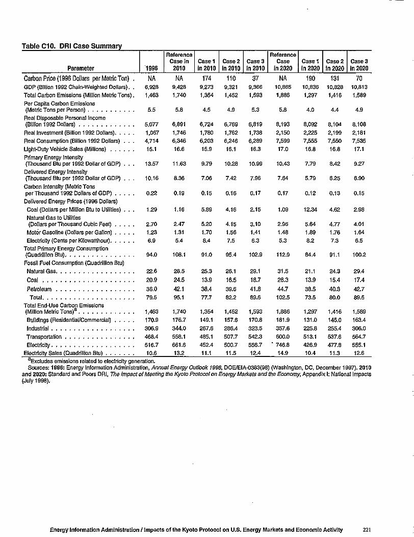
Table C10. DRI Case Summary
Parameter '1996
ReferenceCase in
2010Caseiin 2010
Case 2in 2010
Case 3in 2010
ReferenceCase
in 2020Caseiin 2020
Case 2in 2020
Case 3in 2020
Carbon Price (1996 Dollars per Metric Ton) .GDP (Billion 1992 Chain-Weighted Dollars). .
Total Carbon Emissions (Million Metric Tons).
Per Capita Carbon Emissions(Metric Tons per Person)Real Disposable Personal Income(Billion 1992 Dollars)
Real Investment (Billion 1992 Dollars)
Real Consumption (Billion 1992 Dollars) . . .
Light-Duty Vehicle Sales (Millions)
Primary Energy Intensity(Thousand Btu per 1992 Dollar of GDP) . . .Delivered Energy Intensity(Thousand Btu per 1992 Dollar of GDP) . . .
Carbon Intensity (Metric Tonsper Thousand 1992 Dollars of GDP)
Delivered Energy Prices (1996 Dollars)
Coal (Dollars per Million Btu to Utilities) . . .
Natural Gas to Utilities
(Dollars per Thousand Cubic Feet)
Motor Gasoline (Dollars per Gallon)
Electricity (Cents per Kilowatthour)Total Primary Energy Consumption(Quadrillion Btu)Fossil Fuel Consumption (Quadrillion Btu)
Natural Gas
Coal
Petroleum
TotalTotal End-Use Carbon Emissions(Million Metric Tons)a
Buildings (Residential/Commercial)
Industrial
Transportation
Electricity
Electricity Sales (Quadrillion Btu)
NA6,928
1,463
5.5
5,077
1,067
4,714
15.1
13.57
10.16
0.22
1.29
2.70
1.23
6.9
NA9,428
1,740
5.8
6,891
1,746
6,346
16.6
11.63
8.36
0.19
1.16
2.47
1.31
5.4
1749,273
1,354
4.5
6,724
1,780
6,203
15.9
9.79
7.06
0.15
5.89
5.20
1.70
8.4
1109,321
1,452
4.9
6,769
1,762
6,246
16.1
10.28
7.42
0.16
4.16
4.15
1.56
7.5
379,366
1,593
5.3
6,819
1,738
6,289
16.3
10.99
7.96
0.17
2.15
3.10
1.41
6.3
NA10,865
1,886
5.8
8,193
2,150
7,599
17.0
10.43
7.64
0.17
1.09
2.96
1.48
5.3
19010,836
1,297
4.0
8,092
2,225
7,555
16.8
7.79
5.79
0.12
12.34
5.64
1.89
8.2
13110,828
1,416
4.4
8,104
2,199
7,550
16.8
8.42
6.25
0.13
4.62
4.77
1.76
7.3
7010,813
1,589
4.9
8,108
2,181
7,535
17.1
9.27
6.90
0.15
2.98
4.01
1.64
6.5
94.0 108.1 91.0 95.4 102.9 112.9 84.4 91.1 100.2
22.6
20.9
36.0
79.5
1,463
170.9
306.9
468.4
516.7
10.6
28.5
24.5
42.1
95.1
1,740
176.7
344.0
558.1
661.6
13.2
25.3
13.9
38.4
77.7
1,354
149.1
267.6
485.1
452.4
11.1
26.1
16.5
39.6
82.2
1,452
157.6
286.4
507.7
500.7
11.5
29.1
18.7
41.8
89.6
1,593
170.8
323.5
542.3
556.7
12.4
31.5
26.3
44.7
102.5
1,886
181.9
357.6
600.0
' 746.8
14.9
21.1
13.9
38.5
73.5
1,297
131.0
225.8
513.1
426.9
10.4
24.3
15.4
40.3
80.0
1,416
145.0
255.4
537.6
477.8
11.3
29.4
17.4
42.7
89.5
1,589
163.4
306.0
564.7
555.1
12.6aExcludes emissions related to electricity generation.Sources: 1996: Energy Information Administration, Annual Energy Outlook 1998, DOE/EIA-0383(98) (Washington
and 2020: Standard and Poors DRI, The Impact of Meeting the Kyoto Protocol on Energy Markets and the Economy,(July 1998).
, DC, December 1997). 2010Appendix I: National Impacts
Energy Information Administration / Impacts of the Kyoto Protocol on U.S. Energy Markets and Economic Activity 221

This page Is intentionally left blank.

Appendix D
Letters from the Committee on Science

This page is intentionally left blank.

MHERWOOO L. BOEHICTT. N«w VoltHARROW. FAWEU. IlllnoliC0N8TANCE A. MORELLA, MaiyiindCUBrWElDON, ptniuyfeanlaDANA IIOHRABACHEB, Citfomll8TEVIN SCWfF. N«w MuSooJOE BARTON, T««aaKEN CAIVEAT. CaliforniaROSCOe 0. BARTUTT. MarylandVCTNOHJ.EHUnS.MkhljinDAveWBDON,Horl<!aMATT SALMON, ArljonaTH0UA9 M. DAVIS, VirginiaOil GUTKNECHT, MlimaaeUMASK fOUY. FloridaTHOMAS W. EWINQ. MnobCHARUS W. -CHIT FtOBUNa, MllllulpplCHNS CANNON, UUhKEVMMIAOV.TnuMEJtflU.COOK.UullFHI iNOUSH, PmniySwilaOlOROf R. N6THERCUTT, JiwWatrJnoeonTOM A. COBURN, Oklahomap£TEStSSIONS.TaxM
U.S. HOUSE OF REPRESENTAUVES
COMMITTEE ON SCIENCESUITE 2320 RAYBURN HOUSE OFFICE BUILDING
WASHINGTON, DC 20515^6301(202) 225-6371
TTYM202) 226-4410httpV/wvnv,houM.gov/KfanceAmlcoma.htm
March 3,1998
OEOACE E. BROWK. JIL. CdirwnlaRinUng Minority Monbtr
IUUPHM.HAU.Ttxt>BART GORDON. TrnnwiMJAM|»^TBAFlCANT,J»..Oh!oTIMROEMtR,kiibuROBERT E. (BOO) CRAMER, Jn . AlabamaJAMES A. BARC1A, M I e h S J PPAU.McHAl£. FanmytonUE M * BiRNICE JOHNSON, TaxaaALCEE L HAST1N03, FlorldiIYNNN.HWERS. MichiganZOElCfOREN.Ca»oralaMKXAaF.DOYU. PamaylMnlaSHEKA JACKSON IEX, TuaaBK1 LUTHER, MlnMtoUWALTER H. CAPPS. CalifonJaDEBBIE STABENOW, MlcWginBOS ETHERIOOE, North CarolinaMCKlAMTOON.TaxtaDARUNE HOOUY, OragonEUEN 0. TAinCHER, CalKomla
The Honorable Jay E. HakesAdministratorEnergy Information Administration ..U.S. Department of Energy1000 Independence Avenue, SWWashington, DC 20585
Dear Dr. Hakes:
We appreciated your verbal offer for the Energy Information Administration (EIA) to undertake an analysisof the Kyoto Protocol, particularly focusing on U.S. energy use and prices and the economy in the 2008-2012 time fiame. The purpose of this letter is to confirm that offer and to formally request that analysis. Wewould also like you to include in your study the impact of the penetration of more major efficient technologiesthat are or near commercial availability and other assumptions that have a major bearing on carbonreductions in the United States.
Given the uncertainties that exist regarding the level of carbon reductions that the United States must committo if it is to be in compliance with the Kyoto Protocol, we suggest that several cases be analyzed. Thosecases should bound the possible range of carbon reductions and include intermediate reduction targets thatprovide sufficient information to guide policy decisions. As resources permit, cases should also be examinedthat deal with major policy alternatives in the energy area.
Our staffs will be happy to work with you on this study. We realize that there are numerous alternatives tohow tiie Nation-can proceed to reduce carbon emissions and our mutual discussions of those issues shouldhelp to frame the analysis. We would appreciate the results of your analysis by this fall: In advance, thankyou for your assistance and we commend you and your agency for your consistently reliable energyinformation and analyses.
SENSENBRENNER, JR. GEORGE E. BROWN, JR-Ranking Minority Member
Energy Information Administration / Impacts of the Kyoto Protocol on U.S. Energy Markets and Economic Activity 225

F. JAMES EENSENBRENNER. Jn, Wtaxuln . CHAIRMAN GEORGE E. BROWN. J R . CaliforniaRanking Minority Mamb«r
SHERWOOD L BOEHLERT. Ntw YorkHARRISW. FAYVELMEnoilCONSTANCE A. MOREUA. MarylandCURT WEUDON. PinnsytviniaDANA ROHRABACHER. CalfomiaSTEVEN SCHFF. Nev> MaxicoJOE BARTON. T«xjaKEN CALVERT. CaliforniaROSCOE G. BARTLETT. MarylandVERNON J . EHLERS. MichiganDAVE WELDON, FloridaMATT SALMON, ArinnaTHOMAS M . DAVIS. VirginiaGIL GUTKNECHT, MinnasoUMARK FOLEY. FloridaTHOMAS W . EWINS. nEnoIsCHARLES W . "CHiP- PICKERING. MUaissippICHRIS CANNON. UtahKEVIN BRADY, TaxatMERRIU COOK, UtahPHIL ENGLISH. PannsyfcaniaGEORGE R. NETHERCUTT.JB, WashingtonTOM A. COBURN, OklahomaPETE SESSIONS. Taxla
U.S. HOUSE OF REPRESENTATIVES
COMMITTEE ON SCIENCESUITE 2320 RAYBURN HOUSE OFFICE BUILDING
WASHINGTON, DC 20515-6301
(202)225-6371TTY: (202) 226-4410
http7Avww.house.gov/science/welcome.htm
April 22,1998
RALPH M. HALL TaxasBART GORDON. TanneunJAMES A. TRAFICANT. Ja. OhioTIM ROEMER, IndianaROBERT E, (BUD! CRAMER. Ja , AlabamaJAMES A. BARCIA, MichiganPAUL McHALE. PennsylvaniaEDDIE BERNICE JOHNSON. TaxaaALCEE L HASTINGS, FloridaLYNN N. RIVERS. MichiganZOE LOFGREN. CaliforniaMICHAEL F. DOYLE, PennaytvaniaSHEILA JACKSON LEE. TexaaBILL LUTHER. MinnaaotaWALTER H. CAP PS, CaliforniaDEBBIE STABENOW. MichiganBOB ETHERIDGE. North CarolinaNICK LAMPSON, TaxaaDARLENE HOOLEY, OregonELLEN O. TAUSCHER. California
The Honorable Jay E. HakesAdministratorEnergy Information AdministrationU.S. Department of Energy1000 Independence Avenue, SWWashington, DC 20585
Dear Dr. Hakes:
On March 3, 1998, we formally requested that the Energy Information Administration (EIA) undertakean analysis of the impact of the Kyoto Protocol on U.S. energy use, prices and the economy in the2008-2012 time frame. The purposes of this letter are to more fully define the assumptions for thatstudy and to recommend the specific cases we would like you to consider.
Because of the uncertainties associated with the level of sinks, offsets, emissions of all six greenhousegases, and carbon trading that could result, we would like you to examine several different targets forU.S. energy-related carbon emissions reductions. The plausible cases should span a range of targets,from 7 percent below 1990 levels as the most extreme case to 34 percent above .1990 levels,representing the 2010 emissions level in the Annual Energy Outlook 1998 (AEO98) reference case.Also, for this set of cases we would prefer that you use AEO98 policy, technology and marketassumptions—that is, no additional policies or funding should be assumed unless those changes can bejustified solely based on the existence of the Protocol. Also, the nuclear option should be limited to lifeextension of existing nuclear units, if they are economic.
The recommended cases are:
• 7% below 1990 levels (the Kyoto Protocol target without offsets, sinks and internationaltrading);
• 3% below 1990 levels (State Department estimate of sinks and offsets from reforestation,afforestation, and reductions in other greenhouse gases);
• stabilization at 1990 levels;
• 9% above 1990 levels (State Department estimate of sinks and offsets, plus the EIA estimateof permits available from Annex I countries of the Former Soviet Union);
14% above 1990 levels (stabilization at 1998 emissions levels),

The Honorable Jay E. HakesApril 22, 1998Page two
• 24% above 1990 levels (State Department estimate plus global international trading as definedby Dr. Janet Yellen's testimony of March 4, 1998 before the House Commerce Subcommitteeon Energy and Power); and
• 34% above 1990 levels (EIA reference case levels in AEO98).
With this set of cases, we expect that the EIA will be able to closely estimate the impact on the U.S.energy system and economy for a wide range of values for offsets, sinks, and carbon trading. Forexample, if sinks and offsets from reforestation, afforestation, and reductions in other greenhouse gasesrelax the Kyoto target by 4 percent as the State Department has estimated, and if the United Statescould purchase all of the estimated 165 permits from the Annex I countries of the former Soviet Union,and if no permits were allowed for the Clean Development Mechanism, the carbon target to beexamined for the United States would be 9 percent above 1990 levels, or 1,471 million metric tons.
For each case examined, the target should be achieved on average for the 2008 to 2012 period andstabilize at that target post-2012. You should assume that the United States will begin to respond by2005 to both reflect anticipatory actions by industry and consumers, and to meet the Kyoto Protocol'sArticle 3.2 requirement that "Each Party included in Annex I shall, by 2005, have made demonstrableprogress achieving its commitments under this Protocol."
We would also like you to evaluate other uncertainties regarding: (1) economic growth; (2)construction of new nuclear plants; and (3) technology cost, performance, and penetration as sensitivitycases for some of the target cases described above (e.g., carbon stabilization at 1990 and 1998 levels).
If you have questions concerning these assumptions, please contact Harlan Watson and MikeRodemeyer of the Science Committee staff.
S SENSENBRENNER, JR. GEORGE E. BROWN, JR.an Ranking Minority Member
* U.S. GOVERNMENT PRINTING OFFICE: 1998 433-460/80026
Energy Information Administration / Impacts of the Kyoto Protocol on U.S. Energy Markets and Economic Activity 227