hss2381A – quantitative methods

Univariate Analysis part 2Frequency Analysis

WHAT THE HECK ARE ALL THOSE NUMBERS???

Frequency Distributions

• That’s what a frequency distribution is for—to help impose order on the data

• A frequency distribution is a systematic arrangement of data values, with a count of how many times each value occurred in a dataset

Uses of Frequency Distributions in Data Analysis

• First step in understanding your data!– Begin by looking at the frequency distributions

for all or most variables, to “get a feel” for the data

– Through inspection of frequency distributions, you can begin to assess how “clean” the data are

Data Cleaning

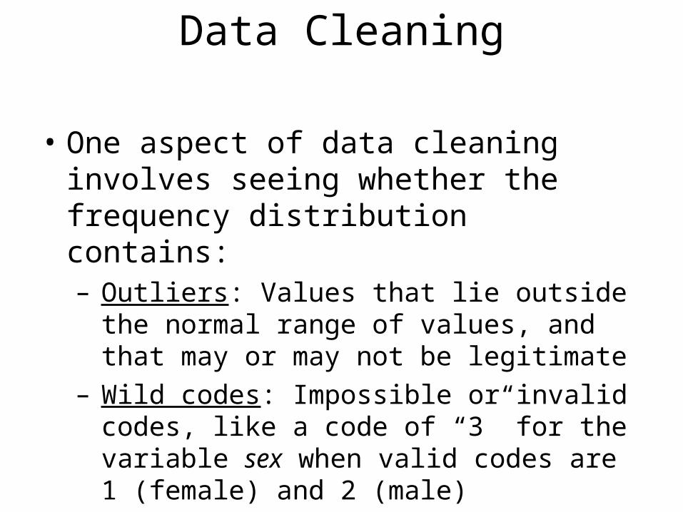
• One aspect of data cleaning involves seeing whether the frequency distribution contains:– Outliers: Values that lie outside the normal

range of values, and that may or may not be legitimate

– Wild codes: Impossible or invalid codes, like a code of “3” for the variable sex when valid codes are 1 (female) and 2 (male)

Wild Codes

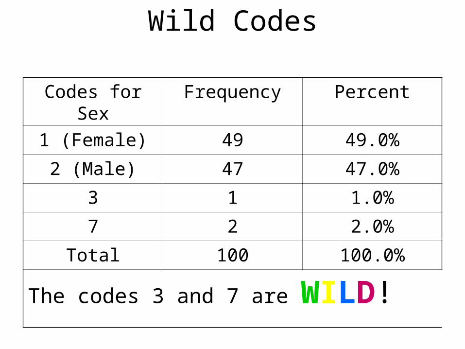
Codes for Sex Frequency Percent

1 (Female) 49 49.0%

2 (Male) 47 47.0%

3 1 1.0%

7 2 2.0%

Total 100 100.0%

The codes 3 and 7 are WILD!

Missing Values

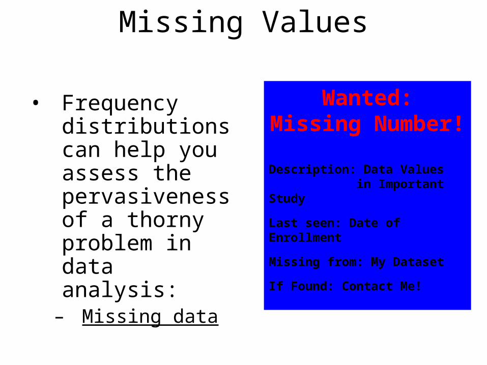
• Frequency distributions can help you assess the pervasiveness of a thorny problem in data analysis:

– Missing data

Wanted:Missing Number!

Description: Data Values in Important Study

Last seen: Date of Enrollment

Missing from: My Dataset

If Found: Contact Me!

Inspection for Missing Values

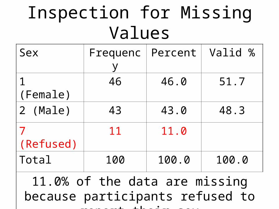
Sex Frequency Percent Valid %

1 (Female) 46 46.0 51.7

2 (Male) 43 43.0 48.3

7 (Refused) 11 11.0

Total 100 100.0 100.0

11.0% of the data are missing because participants refused to report their sex

Assumptions

• Frequency distributions can help you assess validity of certain assumptions for many statistical tests

– An assumption is a condition presumed to be true and, when violated, can result in invalid results

– For many inferential statistics, a normal distribution (for the dependent variable) is assumed

Describe Sample

• Frequency distributions can help you better understand the type of people who are in your study sample:

– What percent are men?– What percent are African American?– What percent have a college degree?

Answer Descriptive Questions

• Frequency distributions can sometimes be used to answer descriptive research questions

• BUT…inferential statistics are almost always needed, because they allow you to draw inferences about a broader group than the study sample

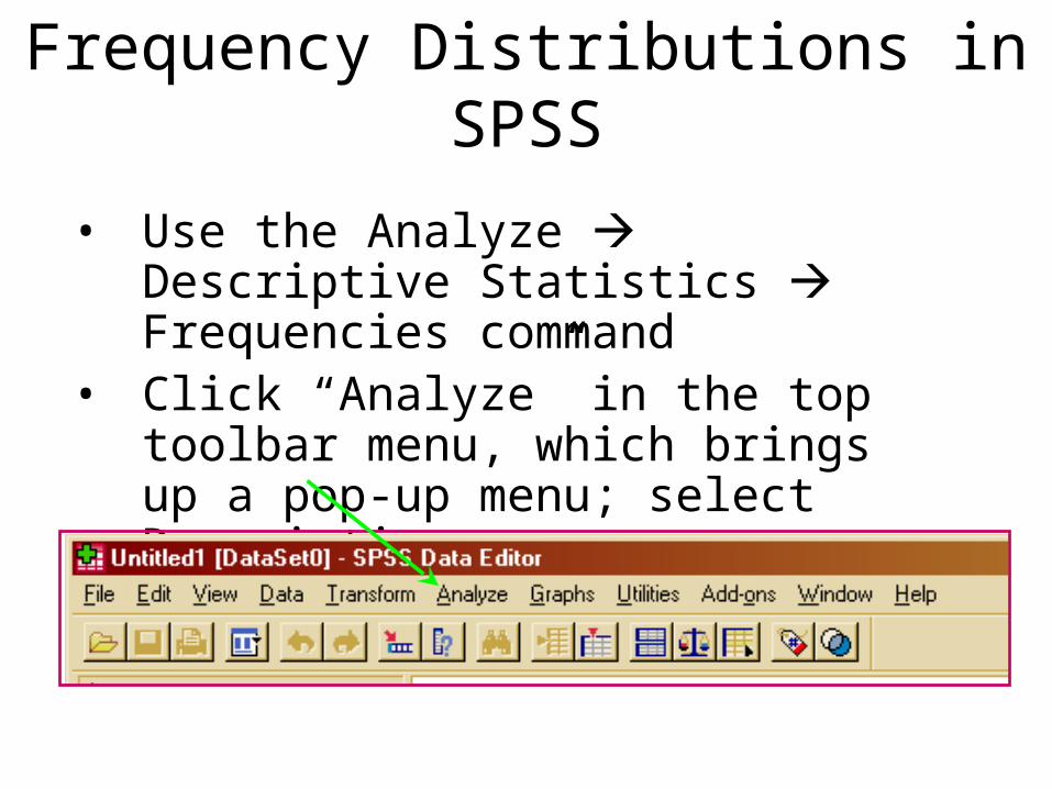
Frequency Distributions in SPSS

• Use the Analyze Descriptive Statistics Frequencies command

• Click “Analyze” in the top toolbar menu, which brings up a pop-up menu; select Descriptives

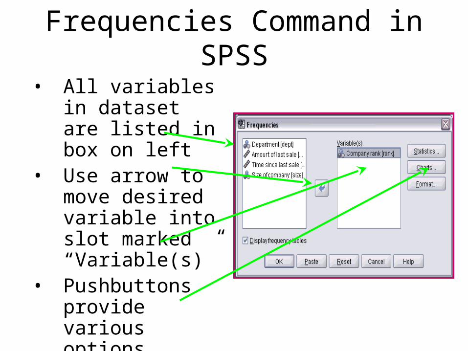
Frequencies Command in SPSS

• All variables in dataset are listed in box on left

• Use arrow to move desired variable into slot marked “Variable(s)”

• Pushbuttons provide various options

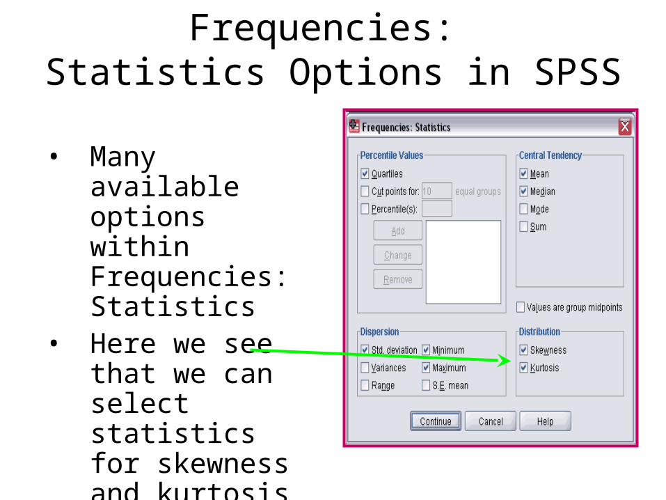
Frequencies: Statistics Options in SPSS

• Many available options within Frequencies: Statistics

• Here we see that we can select statistics for skewness and kurtosis

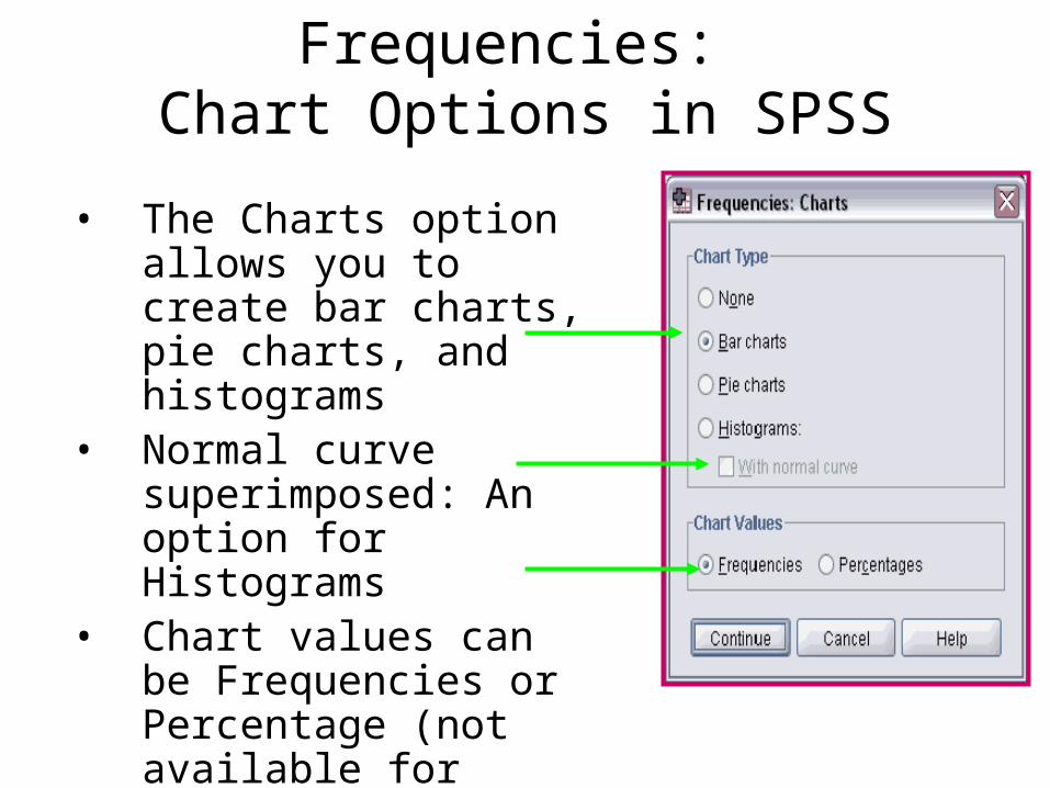
Frequencies: Chart Options in SPSS

• The Charts option allows you to create bar charts, pie charts, and histograms

• Normal curve superimposed: An option for Histograms

• Chart values can be Frequencies or Percentage (not available for Histograms)

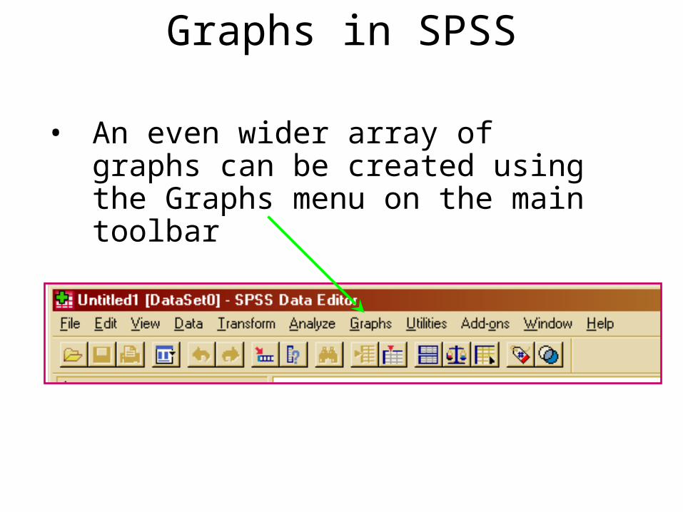
Graphs in SPSS

• An even wider array of graphs can be created using the Graphs menu on the main toolbar

Characteristics of a Data Distribution

• Shape (Chapter 2)• Central tendency• Variability

– Both central tendency and variability can be expressed by indexes that are descriptive statistics

Central Tendency

• Indexes of central tendency provide a single number to characterize a distribution

• Measures of central tendency come from the center of the distribution of data values, indicating what is “typical,” and where data values tend to cluster

• Popularly called an “average”

Central Tendency Indexes

• Three alternative indexes:

– The mode– The median– The mean

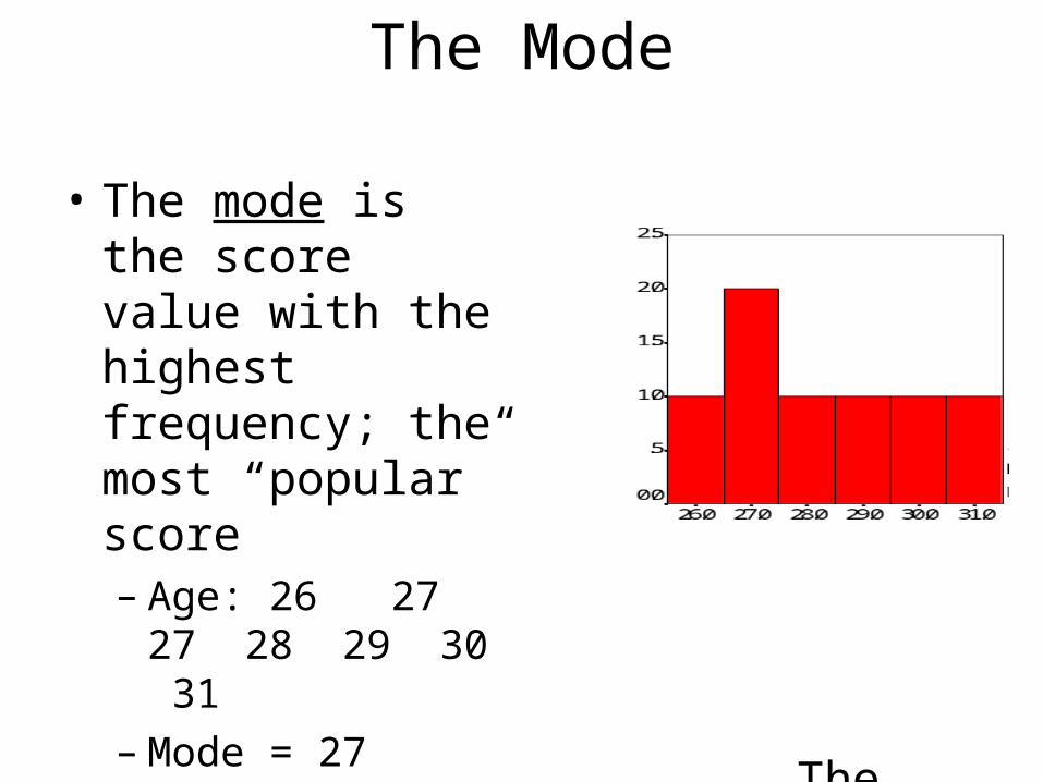
The Mode

• The mode is the score value with the highest frequency; the most “popular” score– Age: 26 27 27 28

29 30 31– Mode = 27

The mode

The Mode: Advantages

• Can be used with data measured on any measurement level (including nominal level)

• Easy to “compute”• Reflects an actual value in the distribution,

so it is easy to understand• Useful when there are 2+ “popular” scores

(i.e., in multimodal distributions)

The Mode: Disadvantages

• Ignores most information in the distribution

• Tends to be unstable (i.e., value varies a lot from one sample to the next)

• Some distributions may not have a mode (e.g., 10, 10, 11, 11, 12, 12)

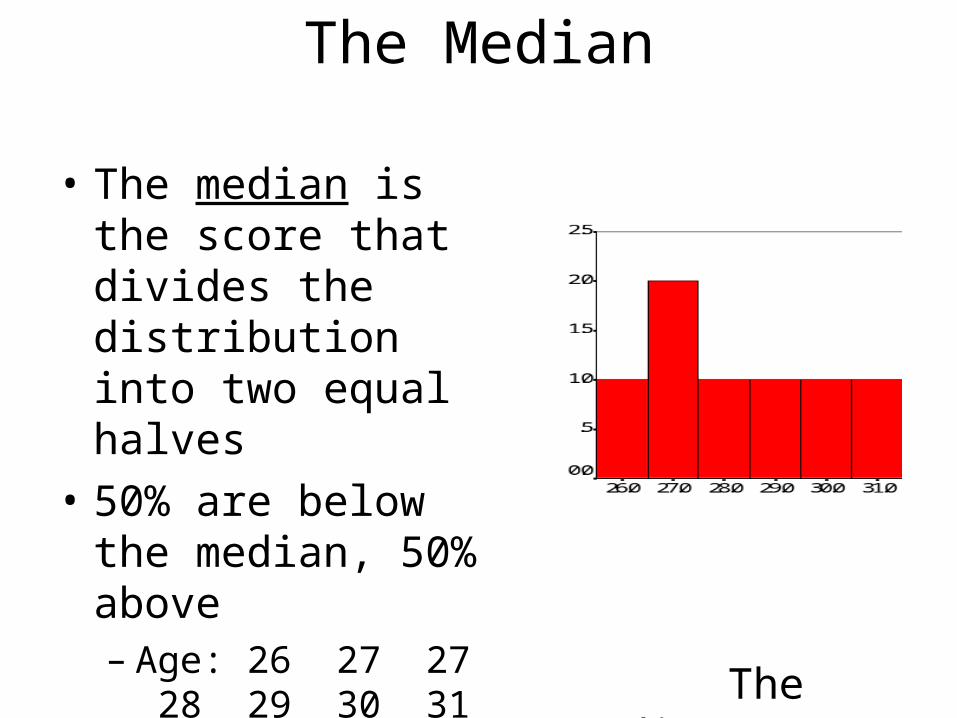
The Median

• The median is the score that divides the distribution into two equal halves

• 50% are below the median, 50% above– Age: 26 27 27 28 29

30 31– Median (Mdn) = 28

The median

The Median: Advantages

• Not influenced by outliers

• Particularly good index of what is “typical” when distribution is skewed

• Easy to “compute”

• Appropriate when data are ordinal level

The Median: Disadvantages

• Does not take actual data values into account—only an index of position

• Value of median not necessarily an actual data value, so it is more difficult to understand than mode

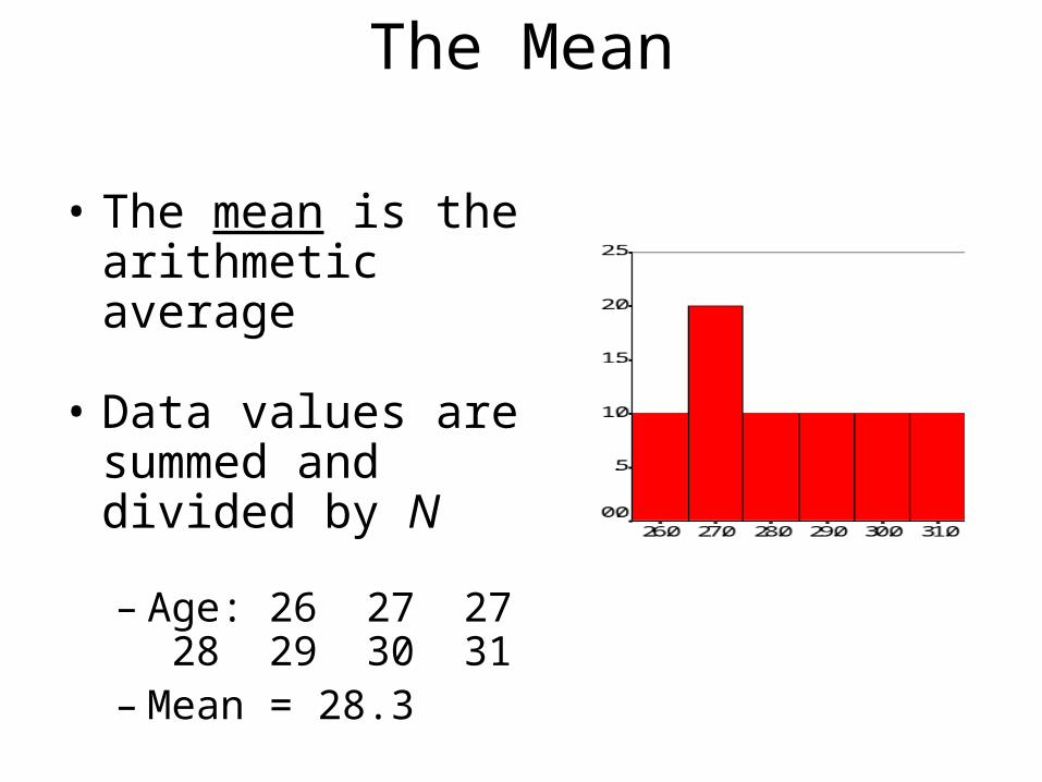
The Mean

• The mean is the arithmetic average

• Data values are summed and divided by N

– Age: 26 27 27 28 29 30 31

– Mean = 28.3 The mean

The Mean (cont’d)

• Most frequently used measure of central tendency—usually preferred for interval- and ratio-level data

• Equation:M = ΣX ÷ N

• Where: M = sample mean Σ = the sum ofX = actual data valuesN = number of people

The Mean: Advantages

• The balance point in the distribution:– Sum of deviations above the mean always

exactly balances those below it

• Does not ignore any information

• The most stable index of central tendency• Many inferential statistics are based on the

mean

The Mean: Disadvantages

• Sensitive to outliers

• Gives a distorted view of what is “typical” when data are skewed

• Value of mean is often not an actual data value

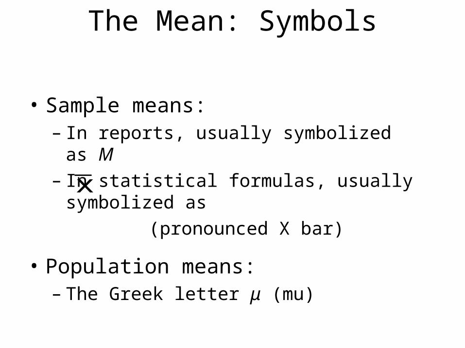
The Mean: Symbols

• Sample means:– In reports, usually symbolized as M – In statistical formulas, usually symbolized as (pronounced X bar)

• Population means:– The Greek letter μ (mu)

x

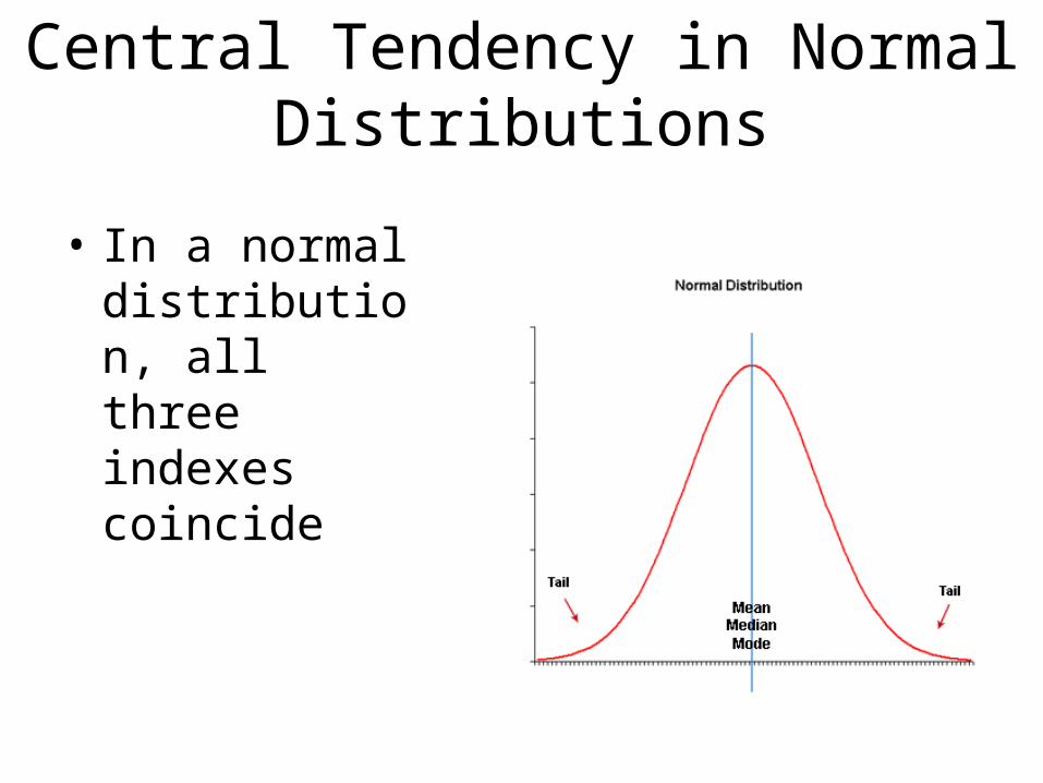
Central Tendency in Normal Distributions

• In a normal distribution, all three indexes coincide

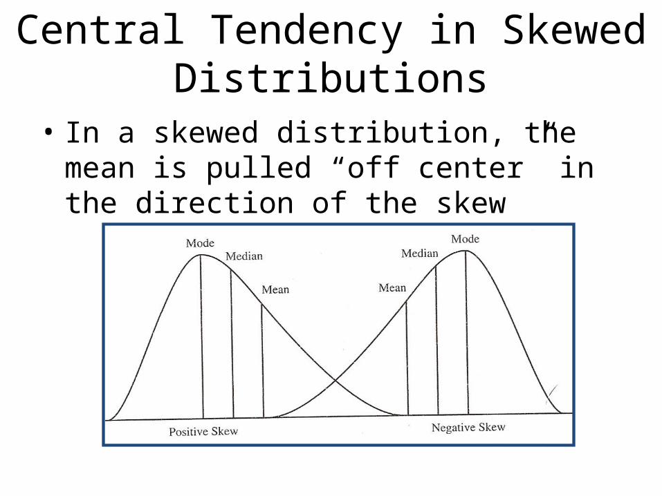
Central Tendency in Skewed Distributions

• In a skewed distribution, the mean is pulled “off center” in the direction of the skew

Variability

• Variability concerns how spread out or dispersed data values in a distribution are

• Two distributions with the same mean could have different dispersion

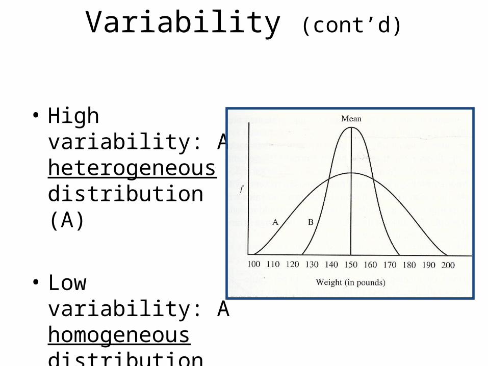
Variability (cont’d)

• High variability: A heterogeneous distribution (A)

• Low variability: A homogeneous distribution (B)

Indexes of Variability

• Range

• Interquartile range

• Standard deviation

• Variance

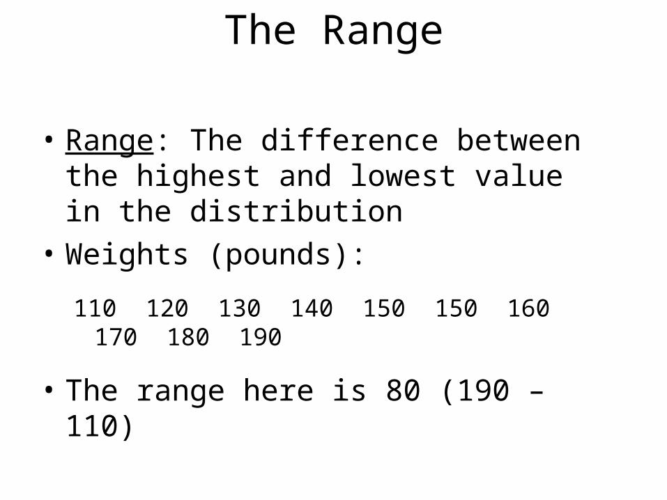
The Range

• Range: The difference between the highest and lowest value in the distribution

• Weights (pounds):

110 120 130 140 150 150 160 170 180 190

• The range here is 80 (190 – 110)

The Range: Advantages

• Easy to compute

• Readily understood

• Communicates information of interest to readers of a report

The Range: Disadvantages

• Depends on only two scores, does not take all information into account

• Sensitive to outliers

• Tends to be unstable—fluctuates from sample to sample

• Influenced by sample size

The Interquartile Range

• Interquartile range (IQR): Based on quartiles– Lower quartile (Q1): Point below which 25% of scores

lie– Upper quartile (Q3): Point below which 75% of scores

lie

• IQR = Q3 - Q1 – IQR is the range of scores within which the middle

50% of scores lie

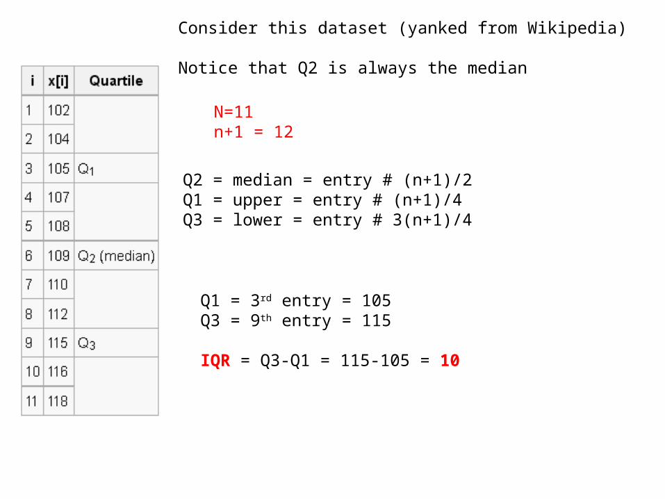
Consider this dataset (yanked from Wikipedia)

Notice that Q2 is always the median

N=11 n+1 = 12

Q2 = median = entry # (n+1)/2Q1 = upper = entry # (n+1)/4Q3 = lower = entry # 3(n+1)/4

Q1 = 3rd entry = 105Q3 = 9th entry = 115

IQR = Q3-Q1 = 115-105 = 10

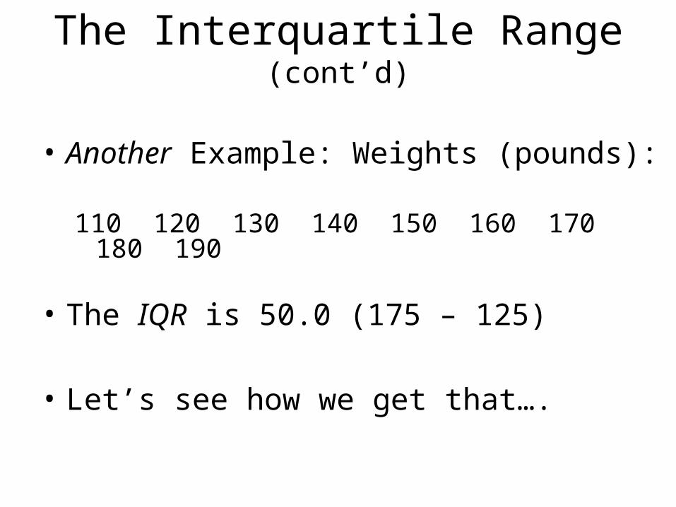
The Interquartile Range (cont’d)

• Another Example: Weights (pounds):

110 120 130 140 150 160 170 180 190

• The IQR is 50.0 (175 – 125)

• Let’s see how we get that….

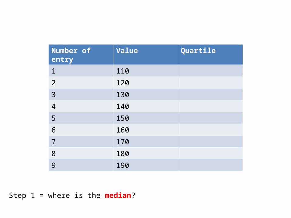
Number of entry Value Quartile

1 110

2 120

3 130

4 140

5 150

6 160

7 170

8 180

9 190

Step 1 = where is the median?

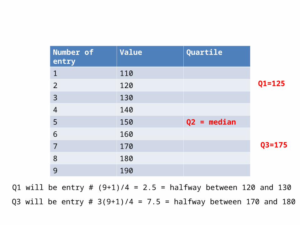
Number of entry Value Quartile

1 110

2 120

3 130

4 140

5 150 Q2 = median

6 160

7 170

8 180

9 190

Q1 will be entry # (9+1)/4 = 2.5 = halfway between 120 and 130

Q1=125

Q3 will be entry # 3(9+1)/4 = 7.5 = halfway between 170 and 180

Q3=175

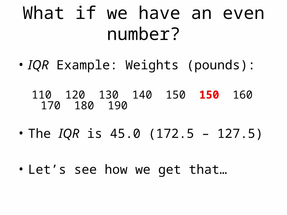
What if we have an even number?

• IQR Example: Weights (pounds):

110 120 130 140 150 150 160 170 180 190

• The IQR is 45.0 (172.5 – 127.5)

• Let’s see how we get that…

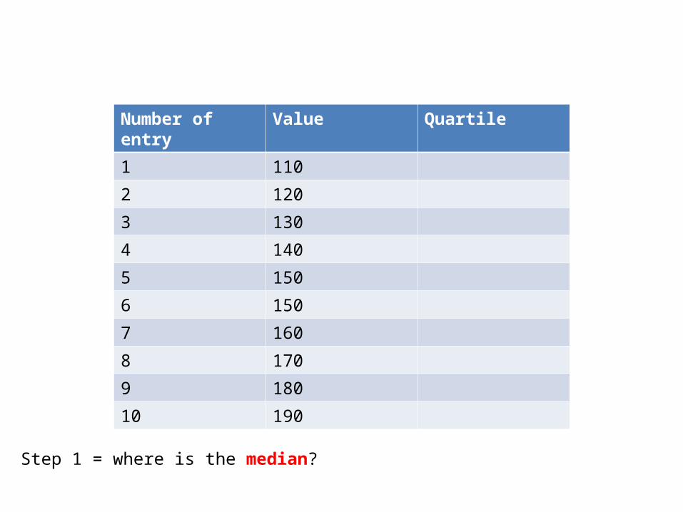
Number of entry Value Quartile

1 110

2 120

3 130

4 140

5 150

6 150

7 160

8 170

9 180

10 190

Step 1 = where is the median?

Number of entry Value

1 110

2 120

3 130

4 140

5 150

6 150

7 160

8 170

9 180

10 190

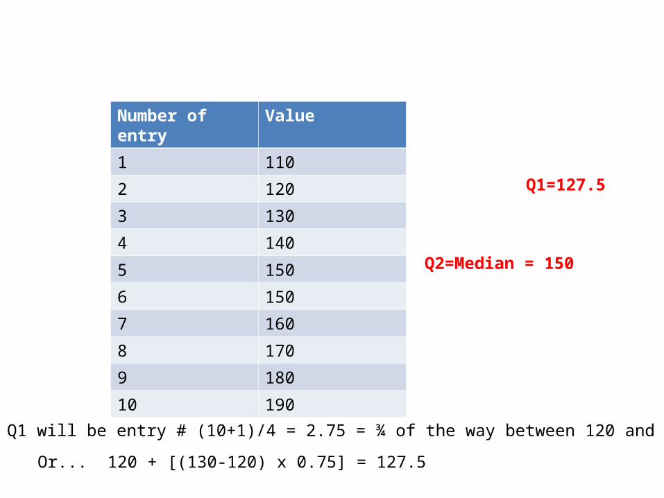
Q1 will be entry # (10+1)/4 = 2.75 = ¾ of the way between 120 and 130

Q1=127.5

Or... 120 + [(130-120) x 0.75] = 127.5

Q2=Median = 150

Number of entry Value

1 110

2 120

3 130

4 140

5 150

6 150

7 160

8 170

9 180

10 190

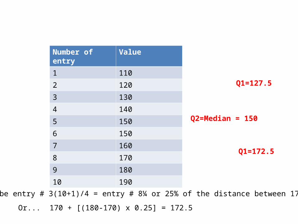
Q3 will be entry # 3(10+1)/4 = entry # 8¼ or 25% of the distance between 170 & 180

Q1=127.5

Or... 170 + [(180-170) x 0.25] = 172.5

Q2=Median = 150

Q1=172.5

Number of entry Value

1 110

2 120

3 130

4 140

5 150

6 150

7 160

8 170

9 180

10 190

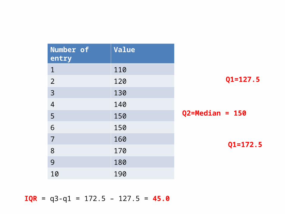
Q1=127.5

IQR = q3-q1 = 172.5 – 127.5 = 45.0

Q2=Median = 150

Q1=172.5

If you want to check your work, use any stats software, or an online IQR calculator, such as:

http://www.alcula.com/calculators/statistics/interquartile-range/

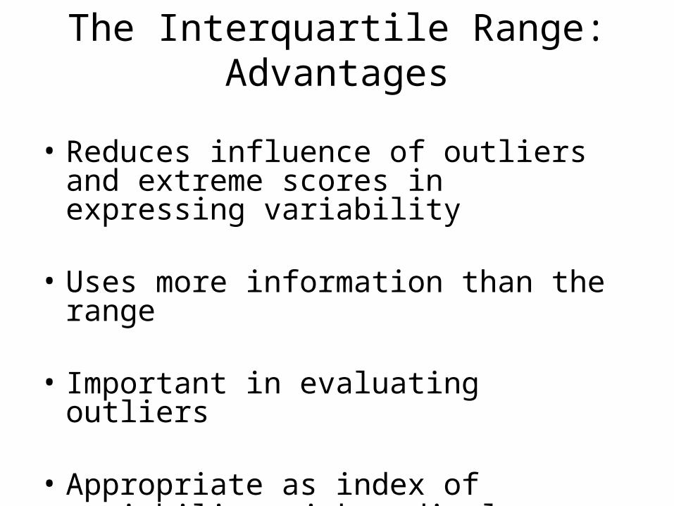
The Interquartile Range: Advantages

• Reduces influence of outliers and extreme scores in expressing variability

• Uses more information than the range

• Important in evaluating outliers

• Appropriate as index of variability with ordinal measures

The Interquartile Range: Advantages

The closer the clustering of values around the median, the smaller the interquartile range

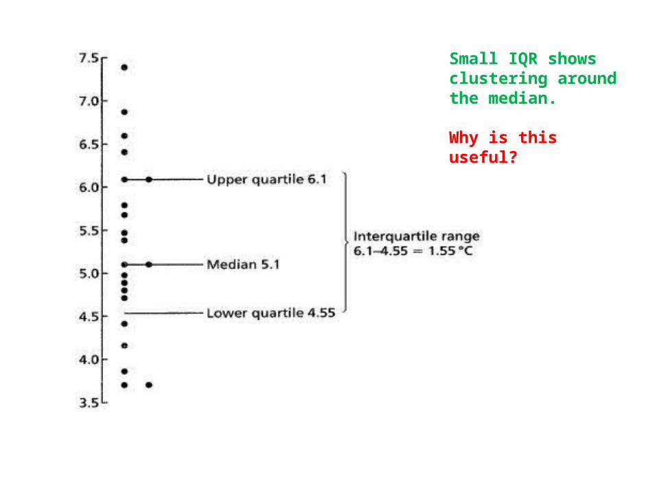
Small IQR shows clustering around the median.

Why is this useful?

The Interquartile Range: Disadvantages

• Is not particularly easy to compute

• Is not well understood

• Does not take all values into account

The Standard Deviation

• Standard deviation (SD): An index that conveys how much, on average, scores in a distribution vary

• SDs are based on deviation scores (x), calculated by subtracting the mean from each person’s original score

x = X - M

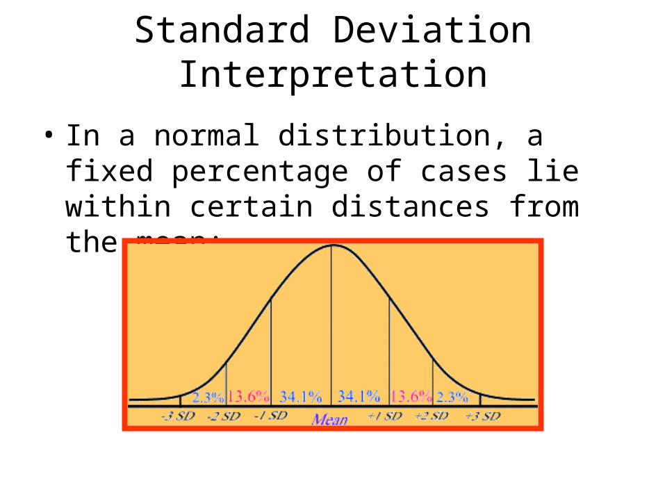
Standard Deviation Interpretation

• In a normal distribution, a fixed percentage of cases lie within certain distances from the mean:

We will do more with SD and variance...

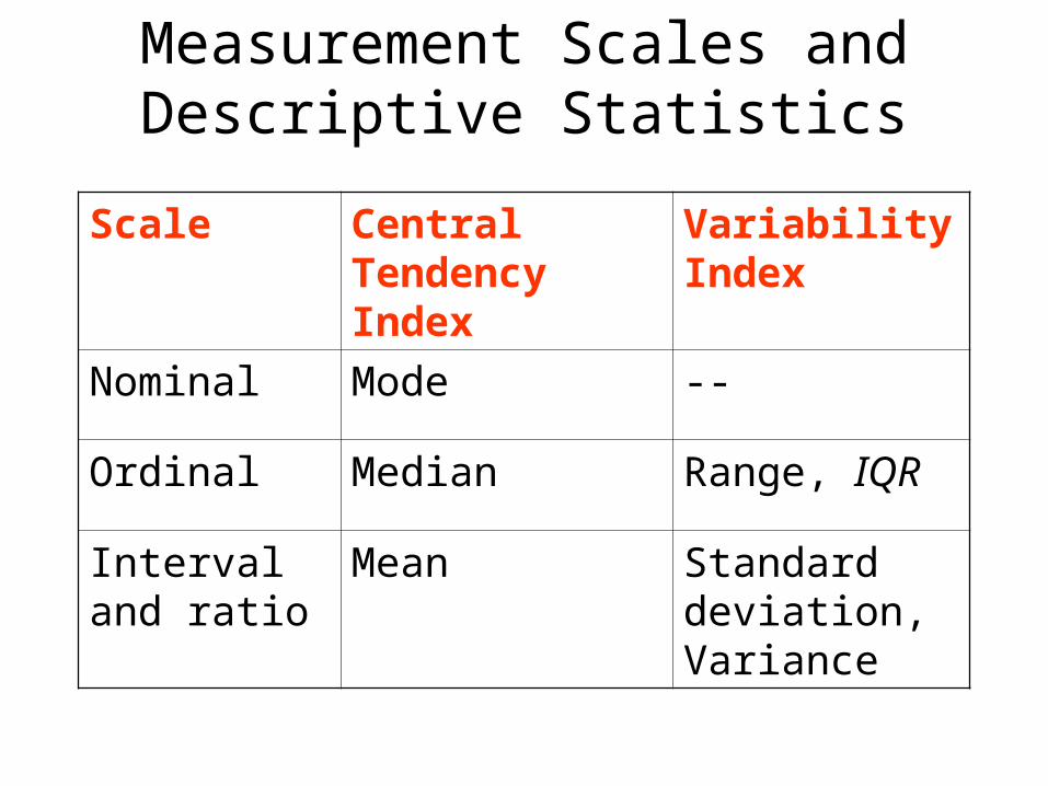
Measurement Scales and Descriptive Statistics

Scale Central Tendency Index

Variability Index

Nominal Mode --

Ordinal Median Range, IQR

Interval and ratio

Mean Standard deviation, Variance

Uses of Descriptive Statistics

• Indexes of central tendency and variability are used to:– Understand data, get a “big picture”– Evaluate outliers and need for strategies to

address problems (e.g., using a trimmed mean that recalculates mean after deleting a fixed percentage (e.g., 5% from either end)

– Describe research participants (e.g., their age, education, length of illness)

– Answer descriptive questions

Descriptive Statistics in SPSS

• Can be obtained through Analyze Descriptive Statistics and are obtained in three programs within that broad umbrella (each has slightly different options):

– Frequencies Statistics– Descriptives Options– Explore Statistics

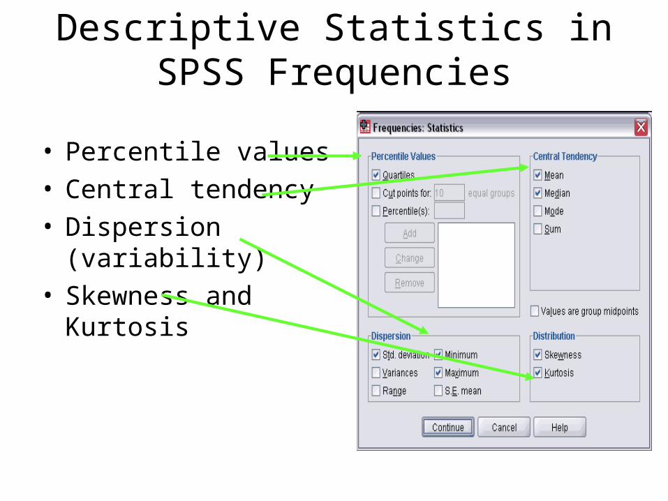
Descriptive Statistics in SPSS Frequencies

• Percentile values• Central tendency • Dispersion (variability)• Skewness and Kurtosis

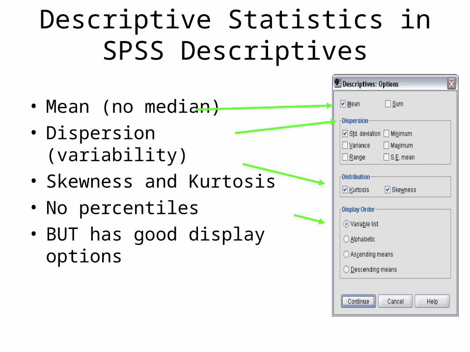
Descriptive Statistics in SPSS Descriptives

• Mean (no median)• Dispersion (variability)• Skewness and Kurtosis• No percentiles• BUT has good display options

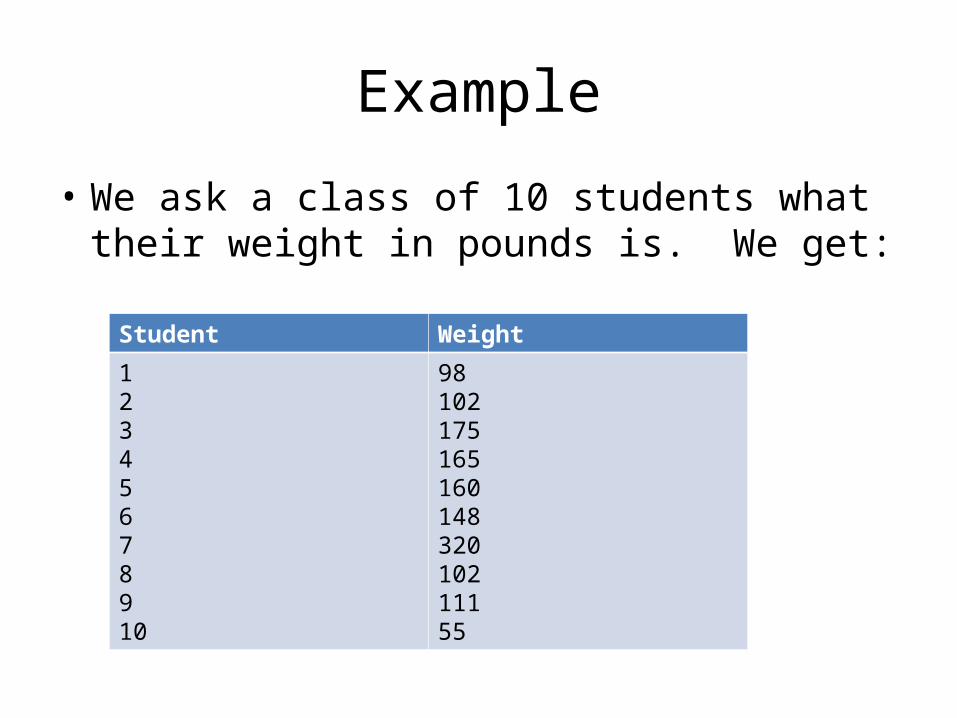
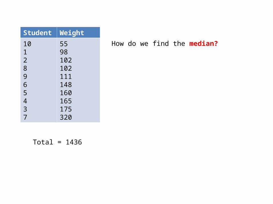
Example

• We ask a class of 10 students what their weight in pounds is. We get:

Student Weight

12345678910

9810217516516014832010211155

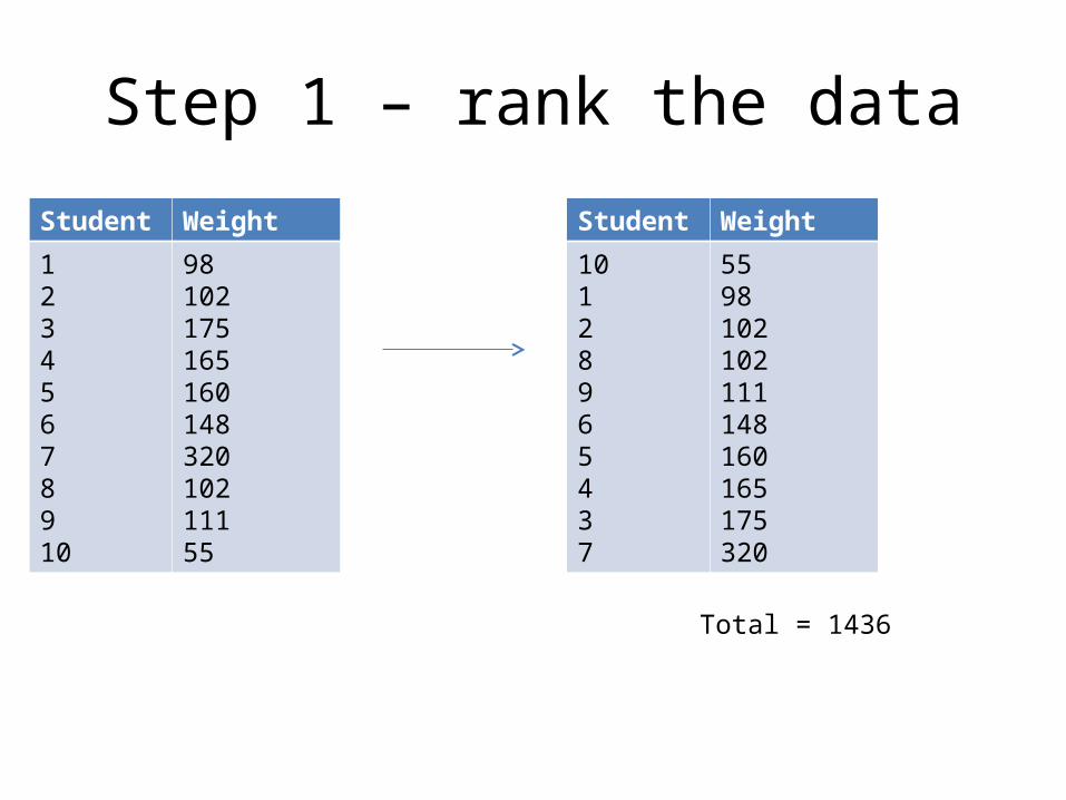
Step 1 – rank the data

Student Weight

12345678910

9810217516516014832010211155

Student Weight

10128965437

5598102102111148160165175320

Total = 1436

Student Weight

10128965437

5598102102111148160165175320

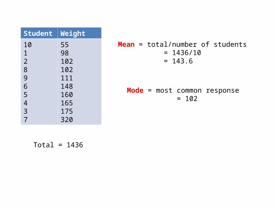
Total = 1436

Mean = total/number of students = 1436/10 = 143.6

Mode = most common response = 102

Student Weight

10128965437

5598102102111148160165175320

Total = 1436

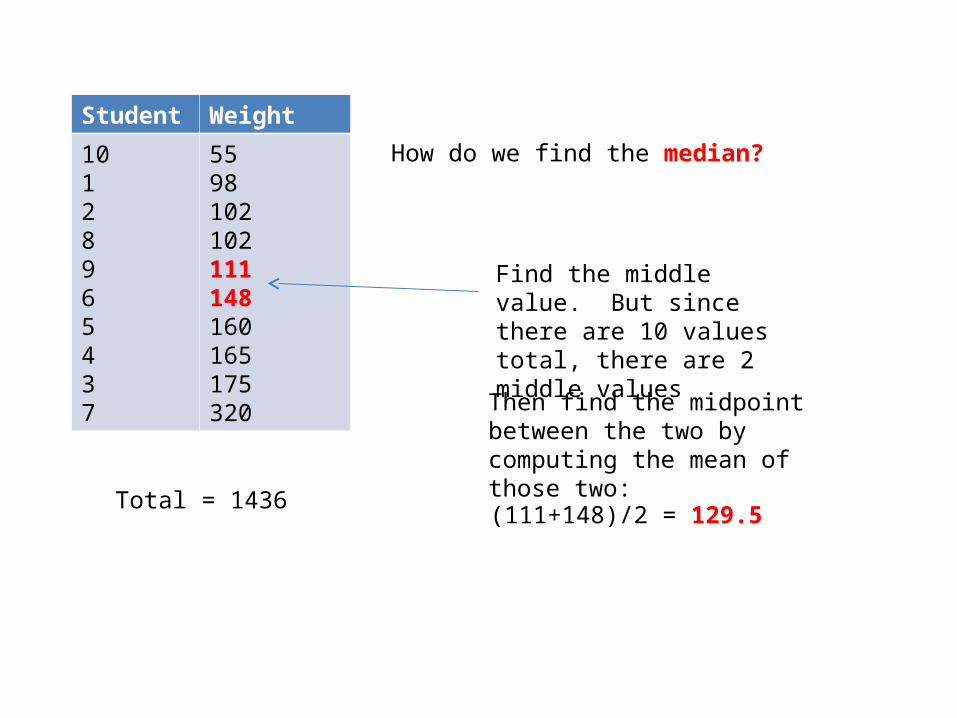
How do we find the median?

Student Weight

10128965437

5598102102111148160165175320

Total = 1436

How do we find the median?

Find the middle value. But since there are 10 values total, there are 2 middle values

Then find the midpoint between the two by computing the mean of those two:

(111+148)/2 = 129.5

Student Weight

10128965437

5598102102111148160165175320

Total = 1436

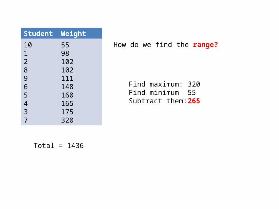
How do we find the range?

Find maximum:Find minimumSubtract them:

32055265

Student Weight

10128965437

5598102102111148160165175320

Total = 1436

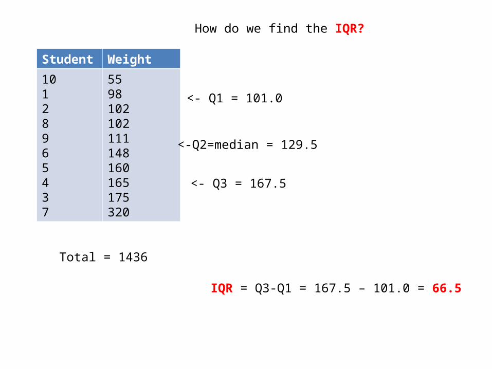
How do we find the IQR?

<-Q2=median = 129.5

<- Q1 = 101.0

<- Q3 = 167.5

IQR = Q3-Q1 = 167.5 – 101.0 = 66.5

Homework

• P. 57 A1, A2, A3