Bivariate analysis

HGEN619 class 2007

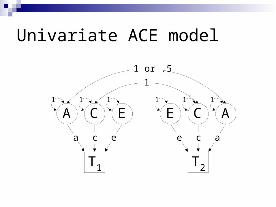
Univariate ACE model

T2

AEA C

a ac e

T1

1 111

E

e

1

C

c

1

1 or .5

1

Expected Covariance Matrices

a2+c2+e2 .5a2+c2

.5a2+c2 a2+c2+e2E DZ =

a 2+c2+e 2 a 2+c2

a 2+c2 a 2+c2+e 2E MZ = 2 x 2

2 x 2

Bivariate Questions I

Univariate Analysis: What are the contributions of additive genetic, dominance/shared environmental and unique environmental factors to the variance?

Bivariate Analysis: What are the contributions of genetic and environmental factors to the covariance between two traits?

Two Traits

EYEX

X Y

AX AYAC

EC

Bivariate Questions II

Two or more traits can be correlated because they share common genes or common environmental influences e.g. Are the same genetic/environmental factors

influencing the traits? With twin data on multiple traits it is possible to

partition the covariation into its genetic and environmental components

Goal: to understand what factors make sets of variables correlate or co-vary

Bivariate Twin Data

individual twin

within between

trait within

between

(within-twin within-trait

co)variance(cross-twin within-trait)

covariance(cross-twin within-trait) covariance

cross-twin cross-trait covariance

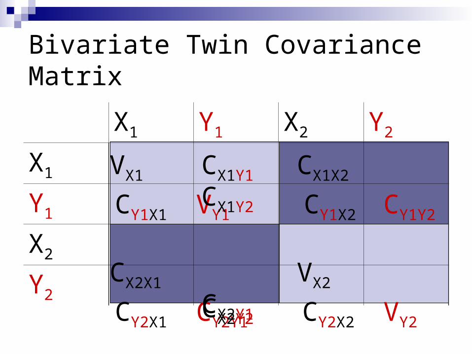
Bivariate Twin Covariance Matrix

X1 Y1 X2 Y2

X1

Y1

X2

Y2

VX1 CX1X2

CX2X1 VX2

VY1 CY1Y2

CY2Y1 VY2

CX1Y1

CX2Y2

CY1X1

CY2X2

CX1Y2

CX2Y1

CY1X2

CY2X1

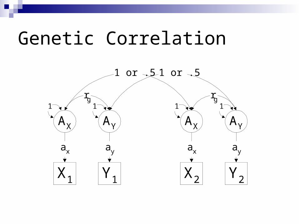
Genetic Correlation

Y2

AYAX AY

ax ayay

X1

1 11

AX

ax

1

1 or .5 1 or .5

X2Y1

rg rg

Alternative Representations

AX AY

ax ay

X1

1 1

Y1

rg

ASX ASY

asx asy

X1

1 1

Y1

AC

1

ac ac

A1 A2

a11 a22

X1

1 1

Y1

a21

Cholesky Decomposition

A1 A2

a11 a22

X1

1 1

Y1

a21

A1 A2

a11 a22

X2

1 1

Y2

a21

1 or .5 1 or .5

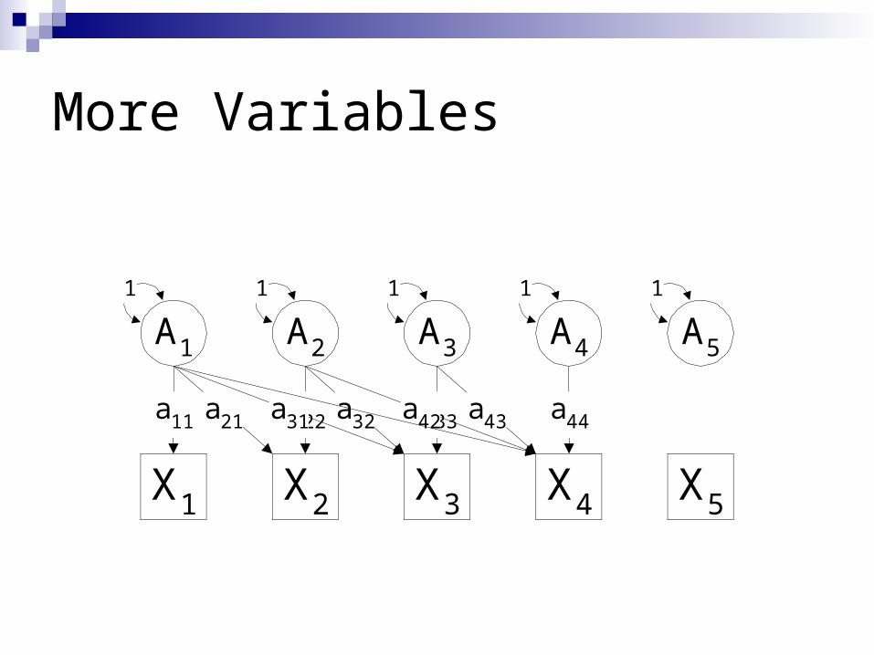
More Variables

A1 A2

a11 a22

X1

1 1

X2

a21

A3

a33

1

X3

A4

a44

1

X4

a32 a43a31 a42

A5

1

X5

Bivariate AE Model

A1 A2

a11 a22

X1

1 1

Y1

a21

A1 A2

a11 a22

X2

1 1

Y2

a21

1 or .5 1 or .5

E1 E2

e11 e22

1 1

e21

E1 E2

e11 e22

1 1

e21

MZ Twin Covariance Matrix

X1 Y1 X2 Y2

X1

Y1

X2

Y2

a112

+e112

a222+a21

2+e22

2+e212

a21*a11+e21*e11

a222+a21

2

a112

a21*a11

DZ Twin Covariance Matrix

X1 Y1 X2 Y2

X1

Y1

X2

Y2

a112

+e112

a222+a21

2+e22

2+e212

a21*a11+e21*e11

.5a222+

.5a212

.5a112

.5a21*a11

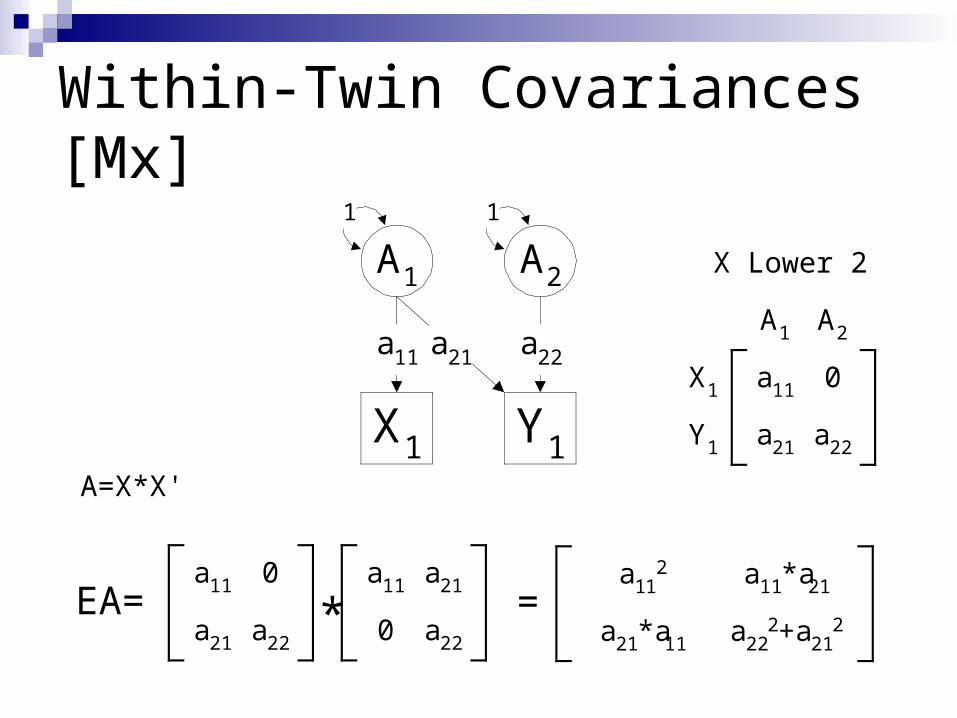
Within-Twin Covariances [Mx]

A1 A2

a11 a22

X1

1 1

Y1

a21a11

a22

0

a21

A1 A2

X1

Y1

X Lower 2 2

a112

a222+a21

2a21*a11

a11*a21=

A=X*X'

a11

a22

0

a21

a11

a220

a21

*EA=

Within-Twin Covariances

Cross-Twin Covariances

a112

a222+a21

2a21*a11

a11*a21EA=MZ

.5a112

.5a222+.5a21

2.5a21*a11

.5a11*a21.5@EA=DZ

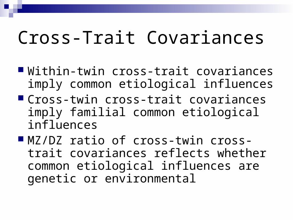
Cross-Trait Covariances

Within-twin cross-trait covariances imply common etiological influences

Cross-twin cross-trait covariances imply familial common etiological influences

MZ/DZ ratio of cross-twin cross-trait covariances reflects whether common etiological influences are genetic or environmental

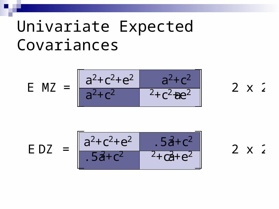
Univariate Expected Covariances

a2+c2+e2 .5a2+c2

.5a2+c2 a2+c2+e2E DZ =

a 2+c2+e 2 a 2+c2

a 2+c2 a 2+c2+e 2E MZ = 2 x 2

2 x 2

Univariate Expected Covariances II

E DZ = EA+EC+EE .5@EA+EC.5@EA+EC EA+EC+EE

EA+EC+EE EA+ECEA+EC EA+EC+EE

E MZ = 2 x 2

2 x 2

Bivariate Expected Covariances

E DZ = EA+EC+EE .5@EA+EC.5@EA+EC EA+EC+EE

EA+EC+EE EA+ECEA+EC EA+EC+EE

E MZ = 4 x 4

4 x 4

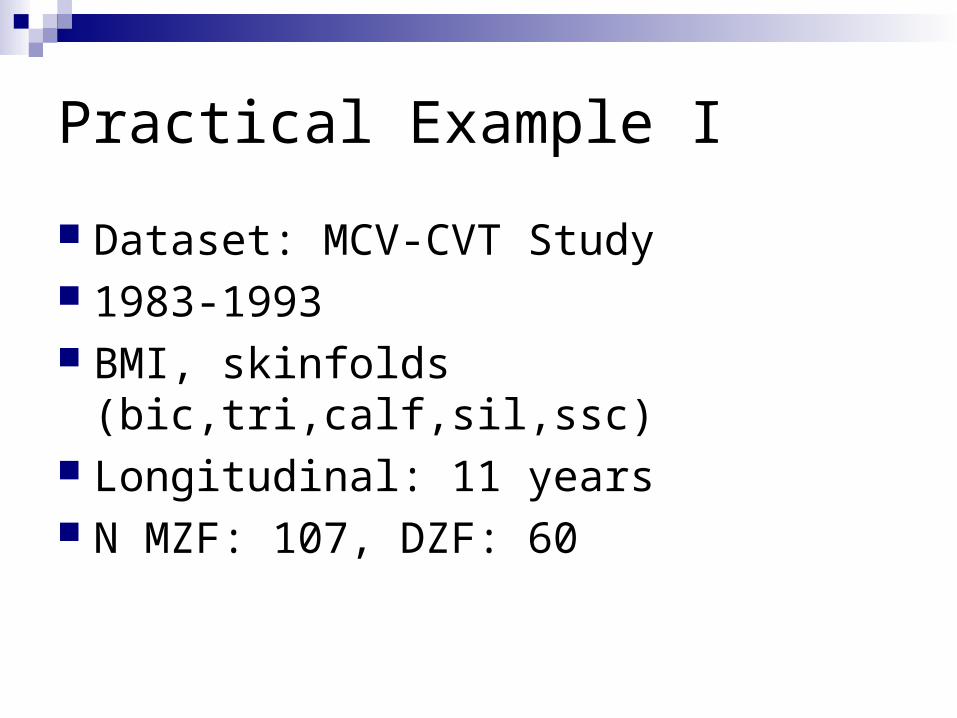
Practical Example I

Dataset: MCV-CVT Study 1983-1993 BMI, skinfolds (bic,tri,calf,sil,ssc) Longitudinal: 11 years N MZF: 107, DZF: 60

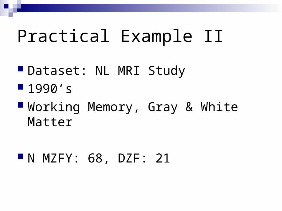
Practical Example II

Dataset: NL MRI Study 1990’s Working Memory, Gray & White Matter

N MZFY: 68, DZF: 21

! Bivariate ACE model! NL mri data I

#NGroups 4 #define nvar 2 ! N dependent variables per twin

G1: Model Parameters Calculation Begin matrices; X Lower nvar nvar Free ! additive genetic path coefficient Y Lower nvar nvar Free ! common environmental path coefficient Z Lower nvar nvar Free ! unique environmental path coefficient H Full 1 1 ! G Full 1 nvar Free ! means End matrices; Matrix H .5 Start .5 X 1 1 1 Y 1 1 1 Z 1 1 1 Start .7 X 1 2 2 Y 1 2 2 Z 1 2 2 Matrix G 6 7 Begin algebra; A= X*X'; ! additive genetic variance C= Y*Y'; ! common environmental variance E= Z*Z'; ! unique environmental variance V= A+C+E; ! total variance S= A%V | C%V | E%V ; ! standardized variance components End algebra; Labels Row V WM BBGM Labels Column V A1 A2 C1 C2 E1 E2 End nlmribiv.mx

! Bivariate ACE model! NL mri data II

G2: MZ twins Data NInputvars=8 ! N inputvars per family Missing=-2.0000 ! missing values ='-2.0000' Rectangular File=mri.rec Labels fam zyg mem1 gm1 wm1 mem2 . .

Select if zyg =1 ;

Select gm1 wm1 gm2 wm2 ; Begin Matrices = Group 1; Means G| G; ! model for means, assuming mean t1=t2 Covariances ! model for MZ variance/covariances A+C+E | A+C _ A+C | A+C+E ; Options RSiduals End

G3: DZ twins Data NInputvars=8 Missing=-2.0000 Rectangular File=mri.rec Labels fam zyg mem1 gm1 wm1 mem2 . . Select if zyg =2 ;

Select gm1 wm1 gm2 wm2 ; Begin Matrices = Group 1; Means G| G; ! model for means, assuming mean t1=t2 Covariances ! model for DZ variance/covariances A+C+E | H@A+C _ H@A+C | A+C+E ; Options RSiduals End

nlmribiv.mx

! Bivariate ACE model! NL mri data III

G4: summary of relevant statistics Calculation Begin Matrices = Group 1 Begin Algebra ; R= \stnd(A)| \stnd(C)| \stnd(E); ! calculates rg|rc|re End Algebra ; Interval @95 S 1 1 1 S 1 1 3 S 1 1 5 ! CI's on A,C,E for first phenotype Interval @95 S 1 2 2 S 1 2 4 S 1 2 6 ! CI's on A,C,E for second phenotype Interval @95 R 4 2 1 R 4 2 3 R 4 2 5 ! CI's on rg, rc, re End

nlmribiv.mx