IZA DP No. 3624

Happiness Inequality in the United States

Betsey StevensonJustin Wolfers

DI

SC

US

SI

ON

PA

PE

R S

ER

IE

S

Forschungsinstitutzur Zukunft der ArbeitInstitute for the Studyof Labor

July 2008

Happiness Inequality in the

United States

Betsey Stevenson Wharton School, University of Pennsylvania,

CESifo and NBER

Justin Wolfers Wharton School, University of Pennsylvania,

CEPR, CESifo, NBER and IZA

Discussion Paper No. 3624 July 2008

IZA

P.O. Box 7240 53072 Bonn

Germany

Phone: +49-228-3894-0 Fax: +49-228-3894-180

E-mail: iza@iza.org

Any opinions expressed here are those of the author(s) and not those of IZA. Research published in this series may include views on policy, but the institute itself takes no institutional policy positions. The Institute for the Study of Labor (IZA) in Bonn is a local and virtual international research center and a place of communication between science, politics and business. IZA is an independent nonprofit organization supported by Deutsche Post World Net. The center is associated with the University of Bonn and offers a stimulating research environment through its international network, workshops and conferences, data service, project support, research visits and doctoral program. IZA engages in (i) original and internationally competitive research in all fields of labor economics, (ii) development of policy concepts, and (iii) dissemination of research results and concepts to the interested public. IZA Discussion Papers often represent preliminary work and are circulated to encourage discussion. Citation of such a paper should account for its provisional character. A revised version may be available directly from the author.

IZA Discussion Paper No. 3624 July 2008

ABSTRACT

Happiness Inequality in the United States*

This paper examines how the level and dispersion of self-reported happiness has evolved over the period 1972-2006. While there has been no increase in aggregate happiness, inequality in happiness has fallen substantially since the 1970s. There have been large changes in the level of happiness across groups: Two-thirds of the black-white happiness gap has been eroded, and the gender happiness gap has disappeared entirely. Paralleling changes in the income distribution, differences in happiness by education have widened substantially. We develop an integrated approach to measuring inequality and decomposing changes in the distribution of happiness, finding a pervasive decline in within-group inequality during the 1970s and 1980s that was experienced by even narrowly-defined demographic groups. Around one-third of this decline has subsequently been unwound. Juxtaposing these changes with large rises in income inequality suggests an important role for non-pecuniary factors in shaping the well-being distribution. JEL Classification: D3, D63, I3, J1, Y1 Keywords: happiness, subjective well-being, inequality Corresponding author: Justin Wolfers The Wharton School University of Pennsylvania 1456 Steinberg-Dietrich Hall 3620 Locust Walk Philadelphia, PA 19104-6372 USA E-mail: jwolfers@wharton.upenn.edu

* The authors would like to thank Wharton’s Zicklin Center for Business Ethics Research and Zell/Lurie Real Estate Center for generous research support.

1

I. Introduction

It is now widely understood that average levels of happiness have failed to grow in the United

States, despite ongoing economic growth (Easterlin, 1995, Blanchflower and Oswald, 2004). Yet an

average can hide as much as it reveals, and so our task in this paper is to explore the full distribution of

happiness through time.

Previous authors have documented the existence of happiness inequality both within and between

demographic groups: the rich are typically happier than the poor; the educated are happier than those with

less education; whites are happier than blacks; those who are married are happier than those who are not;

and women—at least historically—have been happier than men. These differences are likely inter-

related, and additionally, there exists substantial happiness inequality even within narrowly-defined

demographic groups. We seek to document how each of these factors is changing, and how the changing

composition of the U.S. population may be contributing to the observed aggregate trends.

The parallel literature on income inequality certainly suggests that this may be a fruitful task, as

recent decades have witnessed the partial closure of gender and race gaps; education and age gaps have

risen; and income inequality within most demographic groups has risen substantially. All told, this

literature suggests that the gains from recent economic growth have been quite unevenly distributed.

Beyond the pecuniary domain, there have also been important changes in the legal and institutional

organization of work, family, leisure, and community life as well as technological changes that may have

impacted well-being.

As with previous analyses, we find that, on average, happiness has failed to grow since the 1970s.

But beneath this average, we document some important striking differences across groups: Two-thirds of

the black-white happiness gap has been eroded, and the gender happiness gap has disappeared entirely,

with more recent data suggesting that it may even have inverted. Paralleling changes in the income

distribution, differences in happiness by education have widened substantially.

Our more striking finding is the substantial decrease in happiness inequality through our sample.

We document that the dispersion of happiness fell sharply in the 1970s and 1980s; subsequently about

one-third of this decline has subsequently been unwound. Our decomposition exercise suggests that the

real reason for today’s lower levels of happiness inequality is not to be found in the relative experiences

of particular groups, or the specific experiences of only a few, but rather in a pervasive decline in within-

group inequality experienced by even narrowly defined demographic groups.

2

Beyond these substantive findings, our approach to measuring inequality, and our decomposition

of changes in the distribution of happiness within and between groups may be of methodological interest,

especially for those interested in analysis of ordinal data. Our integrated approach to estimating levels

and dispersion of happiness through time and the accounting framework for describing the proximate

sources of these changes may also prove to be useful for analyses of other qualitative or attitudinal data.

Before proceeding, it is worth placing our findings into a broader context. In terms of our

empirical objectives, our goal is to describe the data rather than to point to causal links. We juxtapose

decreasing happiness inequality with rising income inequality not because we believe that this reflects a

clear link between the two, but rather that jointly considered, they hint at the intriguing possibility of a

decline in inequality in the non-pecuniary domain.

The normative implications of our results are also somewhat limited. For instance, a committed

utilitarian cares only about the average level of well-being, and not inequality of well-being. While the

usual utilitarian argument for valuing inequality rests on the view that redistribution yields utility gains to

the poor that exceed the loss to the rich, this argument—based as it is on diminishing marginal utility—

may be more convincing in the pecuniary domain, than when evaluating happiness. We should also add

that the usual caveats about well-being data apply including that the mapping between true subjective

experiences and responses to subjective well-being questions remains quite poorly understood.

Kahneman and Krueger (2006) provide a useful overview of the relevant literature.

Our findings contribute to the much broader (positive) literature on trends in well-being, and

particularly on inequality within the United States. As such, Section II provides the broader context,

describing trends in economic inequality, and in particular its ongoing rise since the 1970s. We also note

that there have been a host of other social and legal changes that may have had interesting distributional

impacts, including changes in the distribution of leisure, regulation impacting families, anti-

discrimination legislation, violent crime, and affirmative action.

In Section III we highlight the aggregate trends in happiness—both levels and dispersion—and

introduce our approach to cardinalizing these descriptive survey responses. Section IV turns to

examining happiness both within and between groups, to assess how the distribution and dispersion of

happiness is changing across socioeconomic and demographic lines. We measure changes in a variety of

dimensions, and assess their joint impact through a decomposition exercise which points to the

importance of within-group rises in happiness inequality. Section V provides a concluding discussion.

3

II. Background: Trends in Inequality

Income inequality has increased throughout our sample period, which begins in 1972. During the

1970s inequality rose modestly, with the rise stemming largely from changes in residual inequality

(Goldin and Katz, The Race Between Education and Technology 2008). The college wage premium fell

through the 1970s, which mitigated against larger rises in overall inequality. However, the college wage

differential rebounded during the 1980s and in this decade inequality rose sharply and throughout the

distribution. The rise in inequality in the 1990s and early 2000s was concentrated in the top of the income

distribution, with the differential between wages at the 90th and 50

th percentiles rising through 2005,

despite a decrease in 50-10 inequality (Autor, Katz and Kearney 2008).

Between 1972 and 2006 (our sample period), overall income inequality rose both within and

between groups with an important part of the rise coming from changes in the returns to education, with

the education returns both increasing and increasing by a greater amount for higher levels of education

(Goldin and Katz 2007). For example, the weekly earnings of full-time, full-year workers with education

beyond a college degree rose 34 log points relative to their counterparts with only a high school degree,

while the parallel rise for those with only a college degree was 22 log points (Goldin and Katz 2008, 139).

Over this period wage dispersion also increased within demographic and skill groups ( (Autor, Katz and

Kearney 2008). In contrast, wage differentials between some groups have narrowed. Specifically, male-

female wage inequality narrowed during the 1970s and 1980s, and continued to narrow, albeit more

slowly, in the 1990 (Blau and Kahn 2006). The black-white wage gap has also narrowed over the past 35

years, with convergence in the 1970s and, after stagnating in the 1980s, further narrowing in the 1990s

(Couch and Daly forthcoming).

Along with this rise in income inequality have come concerns about increasing income volatility,

and a more general concern about increasing inequality stemming from households bearing more health

and retirement risk (Hacker 2006). Income inequality has occurred through both an increase in the

dispersion of permanent income and through an increase in transitory income volatility (Gottschalk and

Moffitt 1994). However, more recent work has argued that increases in income volatility have impacted

few families and have not been broadly experienced (Jensen and Shore 2008).

Since households may be able to use insurance, borrowing, or savings, consumption is less

variable than income, and it may better reflect material well-being. As such, many studies of economic

inequality have turned to measures of consumption inequality, finding evidence of a parallel increase in

consumption inequality in the 1980s (Johnson and Shipp 1997; Cutler and Katz 1991; Attanasio, Battistin

and Ichimura 2004). Some authors have argued, however, that consumption inequality was flat or

4

declining in the 1990s and that the overall rise has been small relative to the rise in income inequality

(Krueger and Perri 2006). The rise in consumption inequality has occurred both between and within skill

groups (Attanasio, Battistin and Ichimura 2004), although this point has been debated in the literature

with Krueger and Perri (2006) suggesting that there was only minimal growth in consumption inequality

within skill groups, despite large increases in within-group income inequality. These same authors find

that between-group changes in consumption inequality have been similar to the between-group changes in

income inequality. Countering this, Johnson and Shipp (1997) argue that most of the rise in consumption

inequality has been within groups.

More recently we have learned that leisure—time devoted to neither market nor household

work— is another important domain in which inequality has changed over recent decades (Aguiar and

Hurst 2007). In particular, the new leisure class is comprised of the low-skilled who have experienced

steady increases in leisure hours over the past three decades. While the high-skilled experienced an

increase in leisure in the 1970s and 1980s, in recent years this increase has been reallocated toward home

production. Yet the biggest rises in non-work, non-household production hours have been among

unemployed and disabled low-skilled men, and most of the increase in “leisure” among those with less

education is due to changes in employment status. In contrast, among men with more education, the

decline in leisure is due to changes within employment status (Aguiar and Hurst 2008).

There have also been important legal changes impacting equality of opportunity. A vast array of

legislation and court rulings have coincided with changes in social norms to reduce discrimination and

allow individuals to make life choices with fewer restrictions due to characteristics such as race, religion,

gender, or sexual preference. Most notably, the 1964 Civil Rights Act outlawed segregation and

discrimination against people on the basis of religion, race, national origin, or gender. This legislation has

continued to impact hiring and firing decisions, with substantial growth in employment discrimination

litigation in the decades since its passage (Donohue and Siegelman 1991). In more recent years,

antidiscrimination legislation has expanded to include the disabled with the Americans with Disabilities

Act of 1990 and the Family and Medical Leave Act of 1993, which protects individuals against job loss in

the case of short-term medical or family issues.

Families have also gained more autonomy over family life with a wave of large-scale

deregulation of the family beginning in the 1960s that diminished the role that government plays in

family life. A series of state legislative changes and constitutional cases in the 1960s and 1970s increased

individual rights surrounding marriage and family, and individuals gained broader access to marriage,

5

divorce, birth control and abortion.2 Many of these legal changes occurred simultaneously with social

upheaval that resulted in large changes in family life. Divorce rates doubled between the mid-1960s and

the mid-1970s, and while they have been falling since the late 1970s, the stock of divorced people has

continued to grow (Stevenson and Wolfers 2007). This increase in the number of people who have

experienced family disruption has increased the dispersion of family experience. Isen and Stevenson

(2008) also document differential changes by education in both family behavior and subjective

assessments of marital satisfaction.

Previous studies of subjective well-being have found that both pecuniary and non-pecuniary

aspects of life contribute to reported happiness. The fact that happiness data aggregate across these

domains makes them especially interesting. Equally, this also expands the range of possible explanations

for the changes in the distribution of happiness we document. In this paper, we refrain from attempting

any such explanation, and we now turn to assessing how the average levels of happiness and happiness

inequality have changed.

III. Aggregate Trends in Happiness

Our analysis is based on responses to the General Social Survey (GSS), which asks: “Taken all

together, how would you say things are these days—would you say that you are very happy, pretty happy,

or not too happy?” This survey was administered to a nationally representative sample of about 1,500

respondents each year from 1972-1993 (except 1979, 1981 and 1992), continued with around 3,000

respondents every second year from 1994 through to 2004, and rose to around 4,500 respondents in 2006

(although only half the respondents were queried about their happiness in 2002 and 2004, followed by

two-thirds in 2006). These repeated cross-sections are designed to track attitudes and behaviors among

the U.S. population and contain a wide range of demographic and attitudinal questions.

Before assessing how answers to these questions have trended over time, it is important to

account for any changes in measurement that may affect responses to the happiness question. While these

data are relatively consistent, responses to happiness questions are remarkably sensitive to small changes

in question order, and hence it is quite important to adjust for changes in survey design. In particular,

Smith (1990) notes that reported happiness tends to be higher when preceded by a five-item satisfaction

scale (as is the norm except 1972 and 1985). Additionally, among married respondents, reported

happiness is higher when preceded by a question about marital happiness (as was the norm, except in

2 See Stevenson and Wolfers (2007) for further discussion of the legal and social changes impacting families during

the 1960s and 1970s.

6

1972). Fortunately the changes induced by these question-order effects can be assessed by way of split-

ballot experiments run in subsequent surveys; Appendix A details these adjustments.3 We show the

results of these corrections in Figure 1.

In order to ensure that these time series are nationally representative, all estimates are weighted

using WTSALL, and we drop the 1982 and 1987 black oversamples. In order to maintain continuity with

earlier survey rounds, we also drop those 2006 interviews that occurred in Spanish and could not have

been completed had English been the only option, as Spanish language surveys were not offered in

previous years.4 Our corrected data series are listed in Table 1.

Having constructed a consistent series, the next challenge is to convert qualitative responses into

a meaningful quantitative summary measure. This issue becomes particularly pressing in analyzing the

GSS data, as only three response categories are given. The simplest (and most widely-used) approach is

to equate “not too happy” with a happiness score of 1, “pretty happy” with a score of 2, and “Very happy”

with a score of 3. We can then take the mean and variance of these measures each year. The results from

this simple approach are presented in Figure 2. Two facts are immediately evident. First, the average

level of happiness in the United States is roughly stable, or perhaps slightly declining, a finding that is

explored further by Blanchflower and Oswald (2004) and subsequently by Stevenson and Wolfers (2008).

Second, inequality in happiness declined until the mid- or late-1980s, despite the fact that both income

and consumption inequality rose through most of this period. Subsequently, happiness inequality rose

through the 1990s, although the most recent estimates of inequality still remain below the higher levels

seen in the early 1970s.5 These movements are quite substantial, as we observe an initial decline in the

variance of happiness of about 25% from the early 1970s to the late-1980s, followed by a rise of about

10% by the mid-2000s.

The difficulty with the aggregation shown in Figure 2 is that it arbitrarily assigns qualitative

categories scores equal to their rank order, imposing a linear structure in which the difference between

being “not too happy” and “pretty happy” is assumed to be equal to the difference between being “pretty

happy” and “very happy”. Moreover, it is difficult to know how to interpret comparisons of happiness

3 While the split ballot experiments provide a bridge between different versions of the survey, they also mean that it

is not possible to simply drop the two outlier years, as results from subsequent surveys also need to be adjusted for

the presence of these experimental split ballots. 4 For those interested in replicating our results, the simplest way is to define a weighting variable as follows: gen

wt=WTSSALL if SAMPLE~=4 & SAMPLE~=5 & SAMPLE~=7 & SPANINT~=2. 5 The decline in happiness inequality from the 1970s to the early 2000s has also been noted by Brooks (2008).

7

levels without some sort of normalization (That is, by what metric can we interpret the economic

significance of the roughly 0.02 point decline in average happiness levels shown in Figure 2?).

An alternative approach involves using data on the proportions of the population who report

themselves as being in each happiness category and imposing a functional form restriction on the

distribution of a latent “happiness” index. A common example of this latter approach is the use of

ordered probit regressions to estimate trends in well-being, as in Stevenson and Wolfers (2007, 2008). In

this approach, one assumes that there is a latent variable, “happiness,” that is normally distributed (and by

an innocuous normalization, it is a standard normal). Thus, an ordered probit regression of happiness on

year fixed effects recovers the time series of the distribution of happiness. This maximum likelihood

procedure simultaneously estimates the “cutpoints” above which a person will report being “pretty

happy” rather than “not too happy,” or “very happy,” rather than “pretty happy.” In turn, the year fixed

effects are interpreted as shifts in the average level of happiness. Unfortunately, the ordered probit (or

ordered logit) is insufficient for our analysis, as we are interested in measuring trends in the dispersion of

happiness, whereas these statistical procedures measure shifts in the average level of happiness, while

assuming its dispersion is constant.

However, it is fairly straightforward to generalize the ordered probit (or ordered logit) in order to

jointly estimate the time series of both the average level and dispersion of happiness. We can also

generalize the specific parameteric assumptions embedded in each particular model. To see this, note that

with three response categories, we have essentially two observations each year—the proportion “not too

happy” and the proportion “very happy” (the proportion “pretty happy” is the complement, and hence

perfectly collinear). Thus we can use these two observations to solve for two unknowns, and hence

recover the parameters of any two-parameter probability density function. 6 Throughout this paper, we

will report the mean and variance of happiness implied by these parameters. We do not mean to suggest

that the variance is the optimal measure of the dispersion of happiness, but given the restriction to two-

parameter distributions, other measures of happiness inequality such as the standard deviation, the Gini

coefficient, interquartile range, and the 90-10 ratio will be a monotonic function of the variance. 7 (For our

purposes the variance is particularly convenient, as the decomposition exercise in Section IV is a

relatively straightforward variance decomposition.)

6 For a related approach, see the appendix to Mankiw, Reis and Wolfers (2003).

7 Atkinson (1970) describes alternative measures of inequality as applying different weights to various parts of the

distribution. In a more applied vein, Kalmjn and Veenhoven (2005) assess different approaches to quantifying

inequality of happiness and conclude by endorsing the use of standard deviations.

8

We begin with the usual logic of the standard models for ordered categorical data, assuming that

the “happiness” of an individual, i, from a representative cross-section taken in period t, is an

unobservable index, ���∗ , determined by:

���∗ = ����� + �� (1)

where ��� refers to the individual’s observable independent variables, and �� is the error term.

However we do not observe ��∗, but rather only observe the ordered categorical variable ��: ��� = �� ��� ℎ���� �� ���∗ ≤ ��

��� = ������ ℎ���� �� �� < ���∗ ≤ ��

��� = ���� ℎ���� �� ���∗ > ��

(2)

where �� and �� are the unknown “cutpoints” that must be estimated.

While the typical ordered probit further assumes ��~(0,1), at this point we generalize in two

directions, allowing for any two-parameter distribution, #(. ) and also allowing the variance to vary with

observable covariates:

��~#(0, ���%�) (3)

Thus the independent variables, ��� , shift both the mean and variance of happiness. We could

allow different sets of independent variables, ���& and ���' to shift the mean and the variance, and this

amounts to denoting the union of these variables as ��� = ���& ∪ ���' and imposing specific zero restrictions

on the � and % vectors. We will not impose such restrictions, because we want to allow the data to

describe which independent variables drive each moment of the distribution.

Because we are interested in using this approach to simply document aggregate time series

variation in the mean and variance of happiness, we begin by focusing on the simple case where the only

independent variables are a vector of year fixed effects, yielding the time series of both the average level

()�) and variance (*��) of happiness. In this particularly simple case, this model yields simple closed-

form expressions, which can be computed without the need for any specialist software. Without

assuming any specific functional form, we note:

%�� ��� ℎ����� = #,-,./0(��) ⇒ #2�(%�� ��� ℎ�����) = �� − )�*� (4)

%���� ℎ����� = 1 − #,-,./0(��) ⇒ #2�(1 − %���� ℎ�����) = �� − )�*� (5)

9

where #(. ) is the cumulative distribution function of a distribution characterized by two

parameters that map into an average level of happiness in each year )� and variance, *��. The key to

identification of this model is that the cutpoints, �� and �� do not vary through time. That is, we can

identify shifts in both the mean and dispersion in happiness, if we are willing to assume that the mapping

between true feelings of happiness and how respondents choose to answer the survey remains constant

through time. (As an aside, while this assumption sounds strong, it is made implicitly in every approach

to cardinalizing subjective well-being that we have seen.) Combining equations (4) and (5) yields:

)� = ��#2�(1 − %���� ℎ�����) − ��#2�(%�� ��� ℎ�����)#2�(1 − %���� ℎ�����) − #2�(%�� ��� ℎ�����) (6)

*�� = 4 �� − ��#2�(1 − %���� ℎ�����) − #2�(%�� ��� ℎ�����)5� (7)

The cutpoints �� and �� define the location and scale over which we are measuring )� and *��,

and so we normalize so as to ensure that the average level of happiness across the entire sample is zero,

and the average variance is one. This normalization implies:

�� = 67 8 #2�(%9:�);�<� (8)

�� = 67 8 #2�(1 − %�:);�<� (9)

where the constant 7 = ;=∑ ?@AB(�2%CD)2@AB(%EFD)GH-IB J0K∑ ?@AB(�2%CD)2@AB(%EFD)GA0H-IB L simplifies

the above expressions, the abbreviations %NTH and %VH correspond to the proportions “not too happy”

and “very happy,” respectively, and τ denotes the number of periods for which we are estimating

happiness trends. Our normalization ensures that we recover estimates of )� and *� that are roughly

comparable across assumptions about functional forms, and comparable to those from an ordered probit

regression (which imposes that this normalization holds for all observations, rather than it just hold on

average).

Thus, for any specific assumption about the functional form of the underlying latent happiness

variable, the simple expressions in equations (6)-(9) can be evaluated using a simple spreadsheet program

10

to compute the time series of both the average level of happiness, and its variance.8 Table 1 provides an

example of these calculations, for the normal distribution.

We assess the robustness of our estimates of the time series of the distribution of happiness in

Figure 3, based on three increasingly fat-tailed assumptions about the distribution of the latent happiness

variable: normality, a logistic distribution, and a uniform distribution. While any set of assumptions will

seem arbitrary, it is worth noting that the more widely-used approach presented in Figure 2 is based on

the particularly unappealing assumption that the happiness distribution has three equally-spaced mass

points corresponding with the three allowable responses.

The key finding is that none of the qualitative (and indeed, quantitative) implications of our

earlier analysis are much changed by alternative approaches to cardinalizing the happiness question,

which is quite reassuring. Again, we find only a mild negative trend in average happiness, but a clear

decline in happiness inequality, with a turning point registered in about the late-1980s, and only a gradual

increase in the subsequent years. By any measure, happiness inequality in the first one-third of our

sample period is higher than in the final third.

Figure 1 provides some simple intuition for why alternative distributional assumptions yield such

similar results: the decline in inequality through to the late 1980s is roughly equally evident whether

looking at those who are unusually happy, or when looking at those who are unusually unhappy, and as

such, placing different weights on the proportion “very happy” relative to the proportion “not too happy”

yields similar trends.

Having found that our simple generalization of the ordered probit, ordered logit and ordered

uniform model yield such similar time series estimate of both the average levels of happiness, and its

dispersion, the rest of our analysis will focus on the generalized ordered probit (which assumes

normality), although none of our results are materially affected by this focus. An alternative rationale for

focusing on the normal distribution is that alternative subjective well-being questions, which elicit

responses on a 10-point scale, tend to yield roughly normally-distributed responses (although as Oswald

(2008) notes, reported happiness reflects the conjunction of true happiness, and an unknown happiness

reporting function).

In order to better assess these changes, we put both mean and dispersion shifts together in

Figure 4, showing the combined impact on the distribution of happiness. In order to keep the charts

8 This computational simplicity is a useful side effect of the model being just-identified. If one were assessing four

or more categorical responses, or were to add control variables, then an explicit maximization routine would be

required. We explore this further in Section IV.

11

uncluttered, we base these plots on decadal averages of the mean and variance of happiness: the decadal

average variance of happiness falls from 1.135 in the 1970s to 0.979 in the 1980s and to 0.897 in the

1990s, before rising to 0.968 in the 2000s; the corresponding numbers for average levels of happiness

show much less movement: 0.015 in the 1970s, 0.015 in the 1980s, -0.023 in the 1990s and -0.024 in the

2000s.9 This plot shows quite clearly that the magnitude of the changes in dispersion dominate any

change in the average level of happiness. For instance, from the 1970s to the 2000s, the happiness level

at the 25th (75

th) percentile of the happiness distribution rose by 0.016 points (fell by 0.094 points),

reflecting a 0.039 point decline in the mean, and a 0.055 point rise (fall) due to increasing happiness

inequality. Indeed, Figure 4 shows that while the decline in average levels of happiness made the

population in the 2000s less happy on average than in the 1970s, the cross-over of the two cumulative

distribution functions implies that 32% of the population are happier today, and this is due to the

offsetting effects of the decline in happiness inequality shrinking the left tail.

Indeed, even as there was not much movement in average levels of happiness in the 1970s and

1980s, there were large rises in happiness at the bottom of the happiness distribution. Figure 5 illustrates,

showing annual estimates of the change in well-being since 1972, at various percentiles of the happiness

distribution. The (unhappiest) 5th percentile have become 0.24 points happier since 1972; the

25th percentile have gained around 0.07 points; the median lost 0.04 points; the 25

th percentile lost

0.16 points, and the (happiest) 5th percentile lost 0.33 points. Again, each of these numbers should be

considered relative to a cross-sectional standard deviation (normalized to one). In order to compare these

magnitudes with their “dollar-equivalents”, note that Stevenson and Wolfers (2008) estimated that each

10 percent rise in log family income is associated with a rise in happiness of 0.022 points.10

Thus, each of

these changes in happiness can be converted to a happiness-equivalent percentage change in income, by

dividing by 0.0022 (or multiplying by 45), suggesting that the decline in happiness inequality that we

document is very large.

In the first column of Table 2, we assess these aggregate trends more formally, analyzing the

annual time series of happiness inequality (and its mean) series derived from our generalization of the

ordered probit. (See the final columns of Table 1 for the underlying data.) Panel A shows decadal-

9 The decades we refer to as the “1970s” should be understood as the period since the General Social Survey began

in 1972; similarly, estimates for the “2000s” reflect data from 2000-2006 (the most recent survey), and the “1980s”

and “1990s” only refers to those years in which the General Social Survey was conducted. 10

The regression reported in Figure 8 of Stevenson and Wolfers (2008) is an ordered probit regression based on

these same 1972-2006 GSS data: Happiness = 0.22*ln(Real family income) [se=0.007], where family income is

deflated by the CPI-U-RS, and each year’s income intervals were converted into point estimates by interval

regressions, assuming that income is log-normally distributed. It should be noted that estimates of the happiness-

income gradient based on other datasets were often somewhat larger, but most tend to lie in the range of 0.2-0.4.

12

averages in happiness inequality, documenting that the variance fell by a total of 15 percent from the

1970s to the 2000s, reflecting a decline of 21 percent from the 1970s through the 1990s, about one-third

of which reversed in the subsequent decade.

Panel B assesses the magnitude and statistical significance of the overall trend in our annual

estimates of inequality. In Panel C, we allow for a change in the trend; in order to minimize data-

snooping (and to maximize statistical power), we simply break the sample in half, testing for a break at

the (chronological) midpoint of our sample, 1989.11

In each case, we report Newey-West standard errors,

accounting for first-order autocorrelation in happiness inequality. These regressions confirm that the

decline in happiness inequality is both economically and statistically significant, and that the average

decline through the sample period reflects a sharp decline in happiness inequality through the first part of

the sample, and a subsequent, smaller, rise in the second part, undoing about one-third of the initial

decline. Panels D, E and F report similar regressions estimates, albeit analyzing average levels of

happiness, rather than its dispersion. These regressions reveal that there is a small, statistically significant

overall decline in average happiness. Average US happiness is lower in the 1990s and 2000s than it was

in the 1970s and 1980s.

Thus far we have shown that in the aggregate happiness inequality fell sharply during the 1970s,

and continued to fall in the 1980s, before rising slightly in the 1990s and 2000s. In contrast, average

happiness in the population shows little evidence of a trend before the late 1980s at which point it falls.

Yet these broad trends may mask underlying heterogeneity in both the average happiness and the

inequality of happiness across socioeconomic and demographic groups. We now turn to digging a bit

further into which groups are most affected by these trends.

IV. Assessing Trends Within and Between Groups

Our approach so far focuses on population aggregates, estimating average happiness and

inequality within each year, by treating annual observations as distinct cells. We can extend our analysis

to consider changes over time within and between categories of demographic groups by estimating

separate regressions that consider demographic category*year as the relevant cell. Formally, this simply

requires replacing the subscript t in equations (4)-(9) (which denoted separate years as the relevant cells),

with the subscript t,d (thus denoting distinct demographic categories in distinct years as the relevant

cells). This procedure yields unconditional estimates of differences in happiness levels and inequality

11

Given the limited degrees of freedom, we do not test for a discontinuous break in levels in the series, allowing

only a change in the trend.

13

both between demographic categories at each point in time, and also within each demographic category,

through time. After estimating these time series, we report a few summary characteristics in Table 2. For

example, by interacting education categories with the year fixed effects, our regression estimates the

average level and variance of happiness in each education category, through time (and indeed, Block II of

Table 2 describes precisely the evolution of happiness by education and time).

Recall that the first column of Table 2 shows the aggregate trends in both happiness and

happiness inequality, and thus summarizes 26 annual observations. Each subsequent block in Table 2

reports separate regressions that analyze separate demographic category by year cells: We first consider

the evolution of happiness by education in Block II, and then turn to assessing trends by gender, racial,

marital, and age groups in subsequent blocks. Note that levels of happiness and the measure of happiness

inequality shown in Table 2 are standardized within each block, and hence are comparable across

columns within a block, but not comparable between blocks. (Estimates within each block are based on

the same cutpoints, but between blocks these are re-estimated, and so differ slightly.) We should also be

clear in noting that these are raw trends, and so they do not simultaneously account for other factors

influencing trends in happiness and happiness inequality.

As such, when interpreting these descriptive analyses—as with all of our demographic

breakdowns—it is important to bear in mind that the dramatic changes in the proportions of the

population choosing higher education levels, or choosing to remain unmarried. If, as seems likely, the

marginal member added to (or subtracted from) each group is different from the average, this changing

composition will account for some of the time series variation in the estimated levels and dispersion of

happiness within each group. This caveat should also be born in mind even in Section IV, as it continues

to be relevant even despite our best efforts to account for observable differences, and compositional

change. Nonetheless, this approach does allow us to make some useful within-group time series

comparisons, and a few interesting trends emerge.

Focusing first on panels A-C, which assess trends in happiness inequality, the most striking

finding is simply that the broad trends seen in the aggregate appear similarly within each of the different

demographic groups. Happiness inequality within most groups was highest in the 1970s, fell in the

subsequent two decades, and rose slightly in the 2000s, although it remains below earlier levels. In

contrast, when looking at the average level of happiness in Panels D, E, and F stark differences occur

across groups.

To examine patterns in each of the groups more closely, we begin by focusing on the patterns by

educational attainment. Recall that returns to education were falling in the 1970s and rose sharply in the

14

1980s, 1990s, and 2000s. Real wages of men with less than a high school degree and those with only a

high school degree stagnated or fell through much of the period, while the real wages of those with a

college degree or beyond rose. In contrast, leisure rose among those with less education relative to those

with more education. Turning to happiness inequality, Columns 2-5 show that, in the 1970s, average

happiness inequality fell with educational attainment. By the 1980s, the differences in happiness

inequality between the groups had declined, such that the gap in the dispersion of happiness between

those with a college degree and those who had attended, but not completed, college had disappeared. In

addition to a decrease in between-group inequality over this period, happiness inequality was much lower

for all groups, except among those who had not completed high school. In the 1990s, happiness

inequality was little changed among those with some college education; it rose for those with a college

degree; and it fell among those with a high school degree or less. In the most recent period, happiness

inequality continued to decline among high school dropouts, despite being higher than the preceding

decade for other groups. By the 2000s, not only was the dispersion of happiness lower within groups

compared with the 1970s, but the differences in happiness inequality between groups had been reduced.

In contrast, Panels D, E, and F of Table 2 show that trends in average levels of happiness has

varied quite strongly across education groups, with happiness rising among college graduates, falling

among those with some college, and falling sharply among those with a high school degree or less. These

patterns are what one might expect based on between-group changes in wage inequality (although it is at

odds with rising leisure among the less-educated).

Turning to examine happiness patterns by gender we see in Panels D, E, and F that women’s

happiness has fallen, while male happiness followed a statistically insignificant upward trend. This

pattern in similar to that seen in Stevenson and Wolfers (2007) who demonstrate that women’s happiness

has fallen both absolutely and relative to that of men since the 1970s. Indeed, the gender happiness gap in

the 1970s was not only eroded over the subsequent decades, but today, women typically report lower

levels of happiness than men. Not surprisingly, happiness inequality for women was also higher than that

for men in the 1970s (Columns 6 and 7 of Panels A, B, and C). Yet inequality among both men and

women fell in roughly equal measure over the next two decades and then rose in the most recent period.

These trends have yielded lower inequality of happiness among both men and women and reduced the

difference in the dispersion of happiness between the two groups.

The racial gap in average happiness has also declined since the 1970s; however non-whites

remain substantially less happy—on average—than whites. We find a strikingly large, statistically

significant increase in the average happiness among non-whites, while happiness among whites has been

15

declining slightly (in columns 8 and 9).12

Examining happiness inequality in the top panels shows that

not only was average happiness much lower among non-whites, but the dispersion of happiness was also

greater. Happiness inequality fell for both groups through to the 1990s and rose in the 2000s; with

inequality lower both within and between racial categories in 2000 compared with the beginning of the

sample.

Lastly, we examine differences in happiness inequality by marital status and by age. One reason

for examining differences across marital patterns is because of the well-known finding that marriage is

associated with higher levels of subjective well-being (Blanchflower and Oswald, 2004). This pattern is

evident in Panel D—in all decades those who are married are happier than those who are not—and there

is little trend in their levels of happiness. Moreover, patterns of inequality of happiness are similar for the

two groups and match the trends seen for the population as a whole.

The final three columns of Table 2 examine patterns by age and here some interesting trends

emerge. The dispersion of happiness increases with age—a fact that is reminiscent of other trends in

inequality by age, such as the fact that dispersion in both income and consumption increases with age

(Deaton and Paxson 1994). However, the rise in happiness inequality over the lifecycle has diminished

over the past 35 years and there is less “fanning out” in the most recent period. The aggregate pattern—

of lower happiness inequality in the 1980s and 1990s, rising in the 2000s—is seen for the youngest and

oldest age groups, although among prime age adults happiness inequality is higher in the 1990s than it is

in the 1980s. The lower panel shows that happiness rises with age, yet the time trend in average

happiness has been flat or slightly rising among the young (aged 18-34) and declining among both prime

age and older adults.13

The key commonality across all of these results is that happiness inequality has declined within

all of these demographic groups. Naturally these trends may be inter-related, and so we conducted a

further analysis based on more narrowly-defined demographic groups, breaking the sample up into 24

sub-samples, reflecting a division into mutually exclusive and collectively exhaustive samples for two

genders, three age groups, and four education levels. Within 20 of these 24 cases we found a trend

decline in happiness inequality and in no case did with find statistically significant evidence of a trend

12

The GSS race variable allows for a division into white, black and “other”. Unfortunately there are so few

respondents in the “other” category that separating non-whites into its constituent groups yields particularly

imprecise, and thus uninformative results for these categories. Even so, in further regressions (not shown) breaking

out these categories, our estimates for blacks largely track those for obtained for the broader “non-white” category. 13

Blanchflower and Oswald (2004) report a “U-shape” in life-cycle happiness in which happiness is highest at

young and older ages. However this pattern is what occurs when examining happiness patterns by age conditional

on life outcomes such as marriage, income, and employment status. Our results in Table 2 are unconditional.

16

increase in inequality. We interpret these findings as suggesting a pervasive rise in within-group

happiness inequality.

Breaking up the sample into distinct sub-samples can only go so far with our limited sample sizes

(and this exercise already yielded some fairly small cell sizes). As such, a more formal regression

framework is needed if we are also going to account for the influence of further factors. We now turn to

developing an appropriate estimation framework in greater detail that will condition on a variety of

demographic and socioeconomic variables at once.

A More General Approach

The key to our estimation is simply to generalize the standard ordered probit so as to allow us to

jointly estimate both the mean and variance of happiness as a function of a rich set of covariates.

Given the model defined by equations (1)-(3), when analyzing a dataset with N observations

indexed by i, a dependent variable consisting of J ordered response categories, and a covariate vector, ���,

the log likelihood function is:

ln O = 8 8 P(��� = Q) ln R# 4�S − �����6���%� 5 − # 4�S2� − �����6���%� 5 TUS<�

E�<�

(10)

where #(. ) is the cdf of the error term and we shall assume that it is normal; we impose no

bounds on the latent happiness variable, and hence �� = −∞ and �U = ∞. Two further constraints are

required to pin down the location and scale of the estimates, and as before, we impose these constraints so

as to ensure that the latent happiness index has a mean of zero, and an average variance of one:

∑ ����� = 0E�<� , and ∑ ���%� = E�<� . Our interest lies in the �� vector, which shifts the average level of

happiness, and %�, which shifts its variance.

Thus, our results in Section III can be re-framed as solving the maximization problem described

by equation (10), where the covariates, ��� were simply a vector of year fixed effects. The advantage of

our generalized framework is that we can now estimate different trends by demographic group,

conditioning on time series movements in the level and dispersion of happiness common to other

demographic characteristics. By comparison, the approach described in equations (4)-(9) required

dividing the sample into mutually exclusive cells—something that is feasible only when assessing a small

number of covariates (particularly given the relatively small samples in the GSS). We now turn to

expanding the vector of relevant covariates, ���, so that it incorporates not only a vector of year fixed

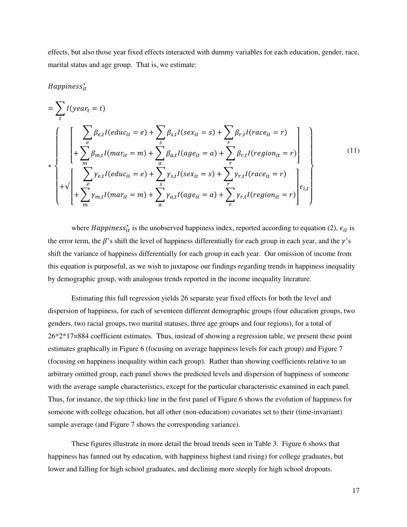
17

effects, but also those year fixed effects interacted with dummy variables for each education, gender, race,

marital status and age group. That is, we estimate:

:����W�XX��∗

= 8 P(����� = �)�

∗

YZZZ[ZZZ\

]̂^̂_ 8 �`,�P(�abc�� = �)

`+ 8 �d,�P(X���� = X)

d+ 8 �e,�P(��c��� = �)

e+ 8 �&,�P(f���� = f)&

+ 8 �g,�P(�h��� = �)g

+ 8 �e,�P(��h��W�� = �)e ij

jjk

+√ ]̂^̂_ 8 %`,�P(�abc�� = �)

`+ 8 %d,�P(X���� = X)

d+ 8 %e,�P(��c��� = �)

e+ 8 %&,�P(f���� = f)&

+ 8 %g,�P(�h��� = �)g

+ 8 %e,�P(��h��W�� = �)e ij

jjk �,�

mZZZnZZZo

(11)

where :����W�XX��∗ is the unobserved happiness index, reported according to equation (2), �� is

the error term, the �’s shift the level of happiness differentially for each group in each year, and the %’s

shift the variance of happiness differentially for each group in each year. Our omission of income from

this equation is purposeful, as we wish to juxtapose our findings regarding trends in happiness inequality

by demographic group, with analogous trends reported in the income inequality literature.

Estimating this full regression yields 26 separate year fixed effects for both the level and

dispersion of happiness, for each of seventeen different demographic groups (four education groups, two

genders, two racial groups, two marital statuses, three age groups and four regions), for a total of

26*2*17=884 coefficient estimates. Thus, instead of showing a regression table, we present these point

estimates graphically in Figure 6 (focusing on average happiness levels for each group) and Figure 7

(focusing on happiness inequality within each group). Rather than showing coefficients relative to an

arbitrary omitted group, each panel shows the predicted levels and dispersion of happiness of someone

with the average sample characteristics, except for the particular characteristic examined in each panel.

Thus, for instance, the top (thick) line in the first panel of Figure 6 shows the evolution of happiness for

someone with college education, but all other (non-education) covariates set to their (time-invariant)

sample average (and Figure 7 shows the corresponding variance).

These figures illustrate in more detail the broad trends seen in Table 3. Figure 6 shows that

happiness has fanned out by education, with happiness highest (and rising) for college graduates, but

lower and falling for high school graduates, and declining more steeply for high school dropouts.

18

Happiness has also become more disperse by age, albeit only slightly. Among 35-49 year olds and those

over 50, happiness has trended downward, while the happiness of 18-34 year olds has trended upward.

As previously seen, happiness has converged along gender and racial lines. Indeed, the closing of the

racial happiness gap is striking and appears to have nearly been eliminated in recent years, suggesting that

the much larger unconditional racial happiness gap seen in Table 2 may be attributable to the combined

impact of racial differences in educational attainment and widening educational differences in

happiness.14

Happiness differences by marital status narrowed in the 1980s, but by the end of the sample

are similar to what were seen in the 1970s. Turning to region in the last panel we see that happiness

trends have been roughly common across space.

Figure 7 shows that the decline in happiness inequality since the 1970s has occurred pretty much

in parallel across demographic groups. There appears to be a fair bit of noise in these annual estimates,

and in no case do the data make a convincing case for sharply different trends in within-group happiness

inequality.

We also present a more compact representation of our results in Table 3, where we analyze

changes by decade, rather than year, so as to reduce the number of coefficient estimates to a manageable

size (and reduce statistical noise). This approach has the advantage of allowing distinct patterns by

decades to be examined for each group. This analysis contains all of the interactions in Table 2 along

with time trends by region, but differs from that table in that it shows conditional estimates. The first

row of Table 3 reports the decadal trends for our baseline group—35-49 year old white, married males

with only a high school degree who live in the Northeast. For this group we see that happiness fell in the

1980s and 1990s, but rose in the 2000s such that there is little difference in happiness between 1972 and

2006 for this group. Among members of this group, inequality in happiness follows the pattern seen in

the aggregate population and is lower in the most recent period compared with the 1970s. To compare

these men with similar men who completed a college degree, we turn to the second row which reports

how the trends differ for college graduates. Adding the second row to the first row provides the trends

35-49 year old white, married males with a college degree who live in the Northeast. Similarly, adding

estimated coefficients for women to those in the top two rows would provide the trends for the equivalent

female.

The estimated trends in Table 3 illustrate that some of the unconditional trends in Table 2 were

reflecting the coincidence of trends in other categories. For example, examining those who are not

14

Again we emphasize differences by demographic group are merely descriptive means (or conditional means) and

it should not be inferred that these are causal relationships.

19

married we see that, conditional on other trends, happiness inequality was higher in the 1980s than in the

1970s, a distinctly different pattern to what we have seen thus far. Yet, the broad trends can still be

seen—happiness is higher among women in the 1970s with the gender gap narrowing in the ensuing

decades. Similarly, happiness is lower among non-whites, yet the gap narrows over the decades. The

dispersion in happiness is higher among women and non-whites in the 1970s, as seen previously.

A Decomposition

The key new finding in this paper is the fact that happiness inequality has declined since the

1970s, even if it has risen somewhat in recent years. In turn, the aggregate trend in happiness inequality

shown in Figure 3 reflects the influence of changing average levels of happiness between groups (shown

in Figure 6), changing happiness inequality within groups (shown in Figure 7), and changing proportions

of the population in each group (Figure 8). In order to assess the combined impact of these separate

influences, we now turn to a decomposition exercise, along the lines suggested by Lemieux (2002).

We begin by noting that our full regression, equation (11), expresses the latent happiness index as

a function of individual characteristics with time-varying coefficients:

:����W�XX��∗ = ����� + 6���%��� (12)

where i denotes the individual observation and t the time period; ��~(0,1) is the error term, ���

is the (1 × q) vector of binary covariates described more fully in equation (11), where the scalar at the jth

position denotes membership in demographic group j, and �� and %� are time-varying (q × 1) vectors of

parameters.

The mean level of happiness in each period can thus be expressed as:

)� = ��r �� (13)

where ��r = ∑ s��� ���/ ∑ s��� is a vector in which the scalar at position j represents the proportion

of the population in period � with characteristic Q, and s�� refers to each observation’s sampling weight. A simple Oaxaca decomposition allows us to describe changes in the mean as due to changes in the time-

varying coefficients versus changes in the composition of the sample:

)� = �u�u + �u?�� − �uG + (��r − �u)�� (14)

where �u = ∑ ∑ s������� / ∑ ∑ s���� is a vector in which the scalar at position j represents the

proportion of the whole sample that has characteristic j. The first term in this expression captures the

average level of happiness in the sample, which is set to zero by our normalization. The second term

captures changes due to time series movements in the average happiness of various groups, captured by

20

deviations of the ��’s from their means. Note that the each of the “within group” changes shown in

Figure 6 are components of this vector, [���, . . , ��v] , and we aggregate these time series into a

representative fixed-weight index by use of a time-invariant weighting vector �u, which describes the

proportions of people in the entire sample with each characteristic. Finally, the impact of changes in the

proportion of the sample with each demographic characteristic is captured by the third term.

We show the estimates of these terms using decadal means in the bottom panel of Block I of

Table 3. The net time series for average happiness is, if anything, somewhat negative over this period.

Yet forming a fixed-weight happiness, �u?�� − �uG, this trend decline disappears. Turning to the final row,

the decadal estimates of the effects of compositional change, (��r − �u)��, illustrate how the population has

shifted into demographic categories that have typically been less happy. In particular, the sample

proportions (in Block III) show the population is increasingly non-white and unmarried—factors

associated with lower happiness—while simultaneously becoming older and more educated—factors

associated with higher average happiness. On aggregate these shifts have contributed to reducing the

overall happiness in the population.

We can also write the variance of :����W�XX��∗ as the sum of “within-group” changes in

happiness, and a component due to changes in happiness levels between groups:

�� = ��r %�x"z{|}{~" + ���Ω|� �������"��|z��~"

(15)

where Ω|� is the variance-covariance matrix of ��� in period t.15

The “within-group” variance can be further decomposed:

��r %� = �u%u + �u(%� − %u) + (��r − �u)%� (16)

where the first term captures the average variance of happiness in our sample, which is set to one

by our normalization. The second term reflects estimated time series movements in the variance within

each group, aggregated using a fixed-weight index. The third term reflects the changes due to changing

composition of the sample into groups prone to greater or lesser degrees of dispersion—a factor

emphasized by Lemieux (2006) as an important explanator of rising residual wage inequality.

15

Note that the literature on wage inequality sometimes refers to the first term in equation (15) as “residual

variance” and the second term as “explained variance”. This terminology reflects the fact that these studies typically

begin by running a regression of wages on observable variables (either in a separate regression for each year, or

alternatively a single regression interacting observable variables with year fixed effects). The second term in

equation (15) is “explained” by these first-stage regressions, while the first term reflects the variance of these

residuals. By contrast, we model shifts in the level and dispersion of happiness in a single step: See equation (11).

21

As with the means, we show the decomposition of the within-group variance using decadal means

in the bottom panel of Table 3 (in Block II). The fixed-weight index of within-group changes in

happiness inequality, �u(%� − %u), point to a substantial decrease in the within group variance of happiness

through to the 1990s. Turning to the estimated (��r − �u)%� term, we see a qualitatively similar pattern—

albeit with a much smaller quantitative contribution— with the changing composition of the sample

contributing to falling dispersion through the 1990s and a rise in dispersion in the 2000s. All told, it

appears that compositional change explains very little of the overall rise in “residual” happiness

inequality.

Finally, the “between-group” variance can be decomposed as follows:

���Ω|��� = �u�Ω���u + ?�� − �uG�Ω��?�� − �uG + ���(Ω|� − Ω��)�� (17)

where �� is the variance-covariance matrix of ��, estimated using data from all time periods.

We combine these time series movements in difference in average levels of happiness between

groups (��, shown in Figure 6), within-group dispersion in happiness (%�, shown in Figure 7), and the

proportion of the population with each demographic (��r , shown in Figure 8) to yield a useful

decomposition of the overall trends in the distribution of happiness, shown in Figure 9.16

This figure

shows that changes in the variance of happiness are being driven more by changes in within group

variance than by changes in between group variance. However, there is a slight downward trend in

between-group variance that is contributing to the overall decrease in happiness inequality since the

1970s. In sum, the figure illustrates while the happiness convergence by race and gender played a role in

reducing inequality, this role was small compared to the overall fall in the inequality of happiness that is

seen within each demographic category.

V. Discussion

While there has been no increase in aggregate happiness over recent decades, there have been

large changes in the level of happiness across groups. Much of the racial happiness gap has closed, the

gender happiness gap has disappeared and perhaps inverted, and differences in happiness by education

have widened substantially. More generally, we document a pervasive decline in happiness since the

16

Of course, alternative decompositions exist, and we can vary the order in which compositional versus within-

group changes are considered or which period to use as the index base (we choose the sample averages, rather than

any specific year). Table 3 provides the raw data necessary for these alternative decompositions; our analysis

suggests that these alternative approaches do not much change the character of our results.

22

1970s, albeit with some reversal over the past decade or so. That these trends differ from trends in both

income growth and income inequality suggests that a useful explanation may lie in the non-pecuniary

domain. As such, we suspect that our data are best interpreted in the broader context of a host of

economic, social, and legal changes impacting equality in the United States over the past 35 years. There

is much more work to be done in unraveling just how these forces are affecting the distribution of

happiness in the United States.

In addition to the changes in both the level and dispersion of happiness between groups, there

have been large demographic shifts which have potentially impacted happiness aggregates. Throughout

this paper we have developed an integrated approach to measuring inequality and decomposing changes

in the distribution of happiness. We examine how the composition and average happiness has changed

both within and between demographic groups, paying particular attention to demographic and

socioeconomic factors known to impact happiness such as education, marital status, age, race, and gender.

This decomposition points to changes in the dispersion of happiness within groups as the main driver of

declining happiness inequality. However while this is a useful accounting exercise, it still leaves

unanswered the question of just what it is that is creating less inequality in the subjectively experienced

lives of demographically-similar people.

References—1

VI. Works Cited

Aguiar, Mark, and Erik Hurst. "Measuring Trends in Leisure: The Allocation of Time Over Five

Decades." Quarterly Journal of Economics, 2007: 969-1006.

Aguiar, Mark, and Erik Hurst. "The Increase in Leisure Inequality." NBER Working Paper 13837,

Cambridge, 2008.

Atkinson, Anthony B. "On the Measurement of Inequality." Journal of Economic Theory 2 (1970): 244-

263.

Attanasio, Orazio, Erich Battistin, and Hidehiko Ichimura. "What Really Happened to Consumption

Inequality in the US." NBER Working Paper 10338, Cambridge, 2004.

Autor, David, Lawrence Katz, and Melissa Kearney. "Trends in U.S. Wage Inequality: Revising the

Revisionists." Review of Economics and Statistics, 2008: 300-323.

Blanchflower, David, and Andrew Oswald. "Well-Being Over Time in Britain and the USA." Journal of

Public Economics 88, no. 7-8 (2004): 1359-1386.

Blau, Francine, and Lawrence Kahn. "The U.S. Gender Pay Gap in The 1990s: Slowing Convergence."

Industrial and Labor Relations Review,, 2006: 45-66.

Brooks, Arthur C. Gross National Happiness: Why Happiness Matters for American—and How We Can

Get More of It. New York: Basic Books, 2008.

Clark, Andrew E., Paul Frijters, and Michael A. Shields. "Relative Income, Happiness and Utility: An

Explanation for the Easterlin Paradox and Other Puzzles." Journal of Economic Literature, forthcoming.

Couch, Kenneth, and Mary Daly. "The Improving Relative Status of Black Men." The Improving Relative

Status of Black Men, forthcoming.

Cutler, David, and Lawrence Katz. "Macroeconomic Performance and the Disadvantaged." Brookings

Papers on Economic Activity, 1991: 1-74.

Deaton, Angus, and Christina Paxson. "Intertemporal Choice and Inequality." Journal of Political

Economy 102, no. 3 (1994): 437-467.

Di Tella, Rafael, Robert J MacCulloch, and Andrew J Oswald. "The Macroeconomics of Happiness."

Review of Economics and Statistics 85, no. 4 (2003): 809-827.

Diener, Ed. Guidelines for National Indicators of Subjective Well-Being and Ill-Being. mimeo, University

of Illinois, 2005.

Donohue, John J., and Peter Siegelman. "The Changing Nature of Employment Discrimination

Litigation." Stanford Law Review 43 (1991): 983.

Easterlin, Richard A. "Does Money Buy Happiness?" The Public Interest 30 (1973): 3-10.

References—2

Easterlin, Richard A. "Will Raising the Incomes of All Increase the Happiness of All?" Journal of

Economic Behavior and Organization 27, no. 1 (1995): 35-48.

Easterlin, Richard A. "Diminishing Marginal Utility of Income? Caveat Emptor." Social Indicators

REsearch 70, no. 3 (2005b): 243-255.

Easterlin, Richard A. "Does economic growth improve the human lot? Some empirical evidence." In

Nations and Households in Economic Growth: Essays in Honor of Moses Abramowitz, by Paul A David

and Melvin W. Reder. New York: Academic Press, Inc., 1974.

Easterlin, Richard A. "Feeding the Illusion of Growth and Happiness: A Reply to Hagerty and

Veenhoven." Social Indicators Research 74, no. 3 (2005): 429-443.

Frey, Bruno S., and Alois Stutzer. "What Can Economists Learn from Happiness Research?" Journal of

Economic Literature 40 (2002): 402-435.

Goldin, Claudia, and Lawrence Katz. "Long-Run Changes in the Wage Structure: Narrowing, Widening,

Polarizing." Brookings Papers on Economic Activity, 2007: 135-165.

—. The Race Between Education and Technology. Cambridge: Harvard University Press, 2008.

Gottschalk, Peter, and Robert Moffitt. "The Growth of Earnings Instability in the US Labor Market."

Brookings Papers on Economic Activity, 1994: 217-272.

Hacker, Jacob. The Great Risk Shift. New York: Oxford University Press, 2006.

Isen, Adam, and Betsey Stevenson. Women's Education and Family Behavior: Trends in Marriage,

Divorce and Fertility. Working Paper, University of Pennsylvania, 2008.

Jensen, Shane, and Stephen Shore. "Changes in the Distribution of Income Volatility." John Hopkins

mimeo, 2008.

Johnson, David, and Stephanie Shipp. "Trends in Inequality Using Consumer Expenditures: 1960 to

1993." Review of Income and Wealth, 1997: 133-152.

Kahneman, Daniel, and Alan B. Krueger. "Developments in the Measurement of Subjective Well-Being."

Journal of Economic Perspectives 20, no. 1 (2006): 3-24.

Krueger, Alan. "Are We Having More Fun Yet? Categorizing and Evaluating Changes in Time

Allocation." Brookings Papers on Economic Activity, forthcoming, 2007.

Krueger, Dirk, and Fanrizio Perri. "Does Income Inequality Lead to Consumption Inequality? Evidence

and Theory." Review of Economic Studies, 2006: 163-193.

Layard, Richard. Happiness: Lessons from a New Science. London: Penguin, 2005.

Layard, Richard. "Human Satisfaction and Public Policy." The Economic Journal, 1980: 737-750.

References—3

Lemieux, Thomas. "Decomposing changes in wage distributions: a unified approach." Canadian Journal

of Economics 35, no. 4 (2002): 646-688.

Lemieux, Thomas. "Increased Residual Wage Inequality: Composition Effects, Noisy Data, or Rising

Demand for Skill." American Economic Review 96, no. 3 (2006): 461-498.

Mankiw, N. Gregory, Ricardo Reis, and Justin Wolfers. "Disagreement About Inflation Expectations."

NBER Macroeconomics Annual, 2003: 209-248.

Oswald, Andrew J. "On the Curvature of the Reporting Function from Objective Reality to Subjective

Feelings." Economics Letters, 2008.

Smith, Tom W. "Time Trends, Seasonal Variations, Intersurvey Differences, and Other Mysteries." Social

Psychology Quarterly 42, no. 1 (1979): 18-30.

Smith, Tom W. Timely Artifacts: A Review of Measurement Variation in the 1972-1989 GSS. GSS

Methodological Report, NORC, Univeristy of Chicago, 1990.

Stevenson, Betsey, and Justin Wolfers. "Economic Growth and Happiness: Reassessing the Easterlin

Paradox." Brookings Papers on Economic Activity, Spring 2008.

Stevenson, Betsey, and Justin Wolfers. "Marriage and Divorce: Changes and Their Driving Forces."

Journal of Economic Perspectives, 2007: 27-52.

Stevenson, Betsey, and Justin Wolfers. The Paradox of Declining Female Happiness. mimeo, University

of Pennsylvania, 2007.

Stevenson, Betsey, and Justin Wolfers. "Trends in Marital Stability." unpublished mimeo, University of

Pennsylvania, 2008.

Wolfers, Justin. "Is Business Cycle Volatility Costly? Evidence from Surveys of Subjective Well-being."

International Finance 6, no. 1 (2003): 1-26.

Appendix—1

Appendix A Correcting for Question Order Effects in the GSS

While the General Social Survey has maintained the same happiness question since its inception

in 1972, responses seem to be quite sensitive to the immediately-preceding battery of questions, and this

ordering has changed several times. We provide this appendix in the hope that it will help the field settle

on a widely-accepted and accurate time series.

There are two key changes in question ordering:

(1) Whether a question probing marital happiness immediately precedes the general happiness

question. (This question is only asked of married couples).

(2) Whether a five-question battery of questions probing domains of satisfaction immediately

precedes the happiness question.

The first context occurs in every year except in 1972, which is replicated in split-ballot

experiments affecting only one-third of the respondents in 1980 and 1987 (those assigned “Form 3”).

Smith (1990) notes that these split ballots suggest that happiness among married respondents tends to be

higher in these instances in which they are preceded by a question about marital happiness.

The second change in question ordering affects all respondents in 1972 and 1985, and its impact

can be assessed by virtue of the fact that it was replicated for 1986 Form 2 respondents and Forms 2 and 3

respondents in 1987. Smith (1990) finds that aggregate happiness is higher in the years in which the

happiness question is preceded by a five-item satisfaction scale.

Because of the split-ballot experiments run in 1980 and 1987—in which one-in-three randomly-

assigned questionnaires dropped the marital satisfaction question—and similar experiments run in 1986

and 1987 in which he satisfaction scale was dropped in one-third and two-thirds of the forms,

respectively, we can assess the changes induced by these question-order effects. These experiments are

particularly useful, in that statistically similar populations are assigned different contexts.

Thus we use these experiments to calculate a set of sampling weights that correct for the under-

sampling of relatively happy people in 1972, 1980 and 1985-87, as well as the oversampling of happy

married people in 1980.

While our analysis largely follows Smith’s suggestions, we differ in two respects. First, we do

not simply drop the experimental forms from the sample, but include their (appropriately-adjusted)

Appendix—2

responses in computing our time series. And second, we also apply a slightly more sophisticated

approach to measuring and correcting for these biases. In particular, given our interest in measuring the

full distribution of happiness, it is important that we provide corrections for the share that are very happy,

pretty happy, and not too happy.

In order to estimate the extent of these biases, we regress happiness on a dummy variable equal to

one for those affected by each sampling change (the first change affected married people in 1972, and

married form 3 respondents in the 1980 and 1987 experiments; the second change affected all 1972 and

1985 respondents, as well as the experimental 1986 form 2 respondents and 1987 form 2 and 3

respondents), controlling for year fixed effects, entered separately for both married and unmarried

respondents. Our dependent variables are separate dummies, corresponding to each of three possible

happiness responses. Thus the ballot experiments identify the effect of changing questionnaire order,

separate from background trends in happiness by marital status. These estimates suggest that the absence

of the marital happiness question led to a statistically significant decline (of about 5.4%) in the proportion

of married respondents reporting themselves “pretty happy”, while the absence of the preceding

satisfaction questions led to a statistically significant rise (of about 2.7%) in the proportion of respondents

claiming they were “not too happy”. The aggregate happiness time series is simply the unadjusted annual

happiness aggregates, less the estimated question order effects (for those subject to the varied question

order). The Stata code required to estimate these effects is available on our homepages.

Finally, in order to ensure that these time series are nationally representative, all estimates are

weighted using WTSALL, and we drop the 1982 and 1987 black oversamples. In order to maintain

continuity with earlier survey rounds, we also drop those interviews that occurred in Spanish, but could

not have been completed had English been the only option.17

17

For those interested in replicating our results, the simplest way is to define a weighting variable as

follows: gen wt=WTSSALL if SAMPLE~=4 & SAMPLE~=5 & SAMPLE~=7 & SPANINT~=2.

Appendix—3

Table A- I: Correcting GSS Happiness Data for Question Order Effects

Year Raw Data Corrected

Not too

happy

Pretty

Happy

Very

Happy

Not too

happy

Pretty

Happy

Very

Happy

Sample

Size

1972 17.2% 53.0% 29.7% 13.6% 49.1% 37.3% 1,606

1973 12.3% 50.9% 36.8% 12.3% 50.9% 36.8% 1,500

1974 12.5% 49.2% 38.3% 12.5% 49.2% 38.3% 1,480

1975 13.0% 53.6% 33.4% 13.0% 53.6% 33.4% 1,485

1976 12.2% 52.9% 34.8% 12.2% 52.9% 34.8% 1,499

1977 11.0% 53.2% 35.7% 11.0% 53.2% 35.7% 1,527

1978 8.4% 56.2% 35.5% 8.4% 56.2% 35.5% 1,517

1980 12.1% 52.6% 35.3% 11.6% 52.0% 36.4% 1,462

1982 11.7% 53.5% 34.8% 11.7% 53.5% 34.8% 1,505

1983 12.1% 56.2% 31.7% 12.1% 56.2% 31.7% 1,573

1984 11.6% 52.1% 36.3% 11.6% 52.1% 36.3% 1,445

1985 10.5% 59.9% 29.6% 8.6% 58.4% 33.1% 1,530

1986 10.2% 56.6% 33.2% 9.2% 55.8% 35.0% 1,449

1987 11.5% 55.0% 33.5% 9.7% 53.3% 37.0% 1,437 1988 8.2% 55.7% 36.1% 8.2% 55.7% 36.1% 1,466

1989 8.8% 56.7% 34.5% 8.8% 56.7% 34.5% 1,526

1990 7.7% 56.5% 35.7% 7.7% 56.5% 35.7% 1,361

1991 9.5% 58.0% 32.5% 9.5% 58.0% 32.5% 1,504

1993 9.7% 56.9% 33.4% 9.7% 56.9% 33.4% 1,601

1994 11.3% 58.2% 30.5% 11.3% 58.2% 30.5% 2,977

1996 10.5% 57.4% 32.1% 10.5% 57.4% 32.1% 2,885

1998 10.9% 55.9% 33.3% 10.9% 55.9% 33.3% 2,806

2000 9.6% 56.4% 33.9% 9.6% 56.4% 33.9% 2,777

2002 11.3% 55.8% 32.9% 11.3% 55.8% 32.9% 1,369

2004 11.7% 54.7% 33.6% 11.7% 54.7% 33.6% 1,337

2006 10.6% 55.9% 33.5% 10.6% 55.9% 33.5% 2,828

Notes: Estimates based on sample weight WTSALL, omitting black oversamples in 1982 and 1987, as well as

those Spanish language interviews in 2006 that could not have been completed were English required (as in

previous years).

“Corrected” series make adjustments in 1972, 1980, 1985, 1986 and 1987 for question-order effects;

affected estimates are shown in bold.

Tables—1

Table 1: Happiness Trends in the United States

Year Survey Responses Estimated moments:

Happiness~N(0,1)

Not too

happy

Pretty

Happy

Very

Happy

Sample

Size

Mean Variance

1972 13.6% 49.1% 37.3% 1,606 0.023 1.321

1973 12.3% 50.9% 36.8% 1,500 0.027 1.194

1974 12.5% 49.2% 38.3% 1,480 0.060 1.279

1975 13.0% 53.6% 33.4% 1,485 -0.055 1.106

1976 12.2% 52.9% 34.8% 1,499 -0.015 1.112

1977 11.0% 53.2% 35.7% 1,527 0.020 1.059

1978 8.4% 56.2% 35.5% 1,517 0.048 0.871

1980 11.6% 52.0% 36.4% 1,462 0.027 1.123

1982 11.7% 53.5% 34.8% 1,505 -0.008 1.072

1983 12.1% 56.2% 31.7% 1,573 -0.078 0.988

1984 11.6% 52.1% 36.3% 1,445 0.025 1.123

1985 8.6% 58.4% 33.1% 1,530 -0.001 0.821

1986 9.2% 55.8% 35.0% 1,449 0.026 0.912

1987 9.7% 53.3% 37.0% 1,437 0.060 1.016

1988 8.2% 55.7% 36.1% 1,466 0.061 0.880

1989 8.8% 56.7% 34.5% 1,526 0.023 0.872

1990 7.7% 56.5% 35.7% 1,361 0.061 0.838

1991 9.5% 58.0% 32.5% 1,504 -0.025 0.861

1993 9.7% 56.9% 33.4% 1,601 -0.011 0.900

1994 11.3% 58.2% 30.5% 2,977 -0.089 0.904

1996 10.5% 57.4% 32.1% 2,885 -0.047 0.909

1998 10.9% 55.9% 33.3% 2,806 -0.030 0.967

2000 9.6% 56.4% 33.9% 2,777 0.000 0.909

2002 11.3% 55.8% 32.9% 1,369 -0.043 0.979

2004 11.7% 54.7% 33.6% 1,337 -0.034 1.029

2006 10.6% 55.9% 33.5% 2,828 -0.019 0.955

Source: General Social Survey, 1972-2006.

Notes: Estimates based on sample weight WTSALL, omitting black oversamples in 1982 and 1987, as well as

those Spanish language interviews in 2006 that could not have been completed were English required (as in

previous years).

All data are corrected for question order effects, as described in Appendix A.

The mean and variance estimates are based on a generalized ordered probit regression of happiness in

which both the level and variance of happiness are a linear function of year fixed effects, as described in

equations (6)-(9). These estimates are constructed on the assumption that the latent happiness variable is

normally distributed, with mean zero, and average variance equal to one. The estimated cutpoints are �� = −1.244 and �� = 0.397.

Tables—2

Table 2: Trends in Happiness Inequality and Levels, by Group

Block I:

ALL

Block II:

By Education

Block III:

By Gender

Block IV:

By Race

Block V:

By Marital Status

Block VI:

By Age

Whole

Sample

College

grad

Some

college

High

school

<High

School

Men Women White Non-

White

Married Not

married

18-34 35-49 50+

TRENDS IN HAPPINESS INEQUALITY

Variance of Happiness (Relative to sample average)

Panel A: Decadal Averages of SD(happiness)

1970s 1.135 0.921 1.053 1.126 1.316 1.073 1.200 1.049 1.223 1.186 1.045 1.001 1.113 1.270

1980s 0.979 0.836 0.840 0.917 1.316 0.958 0.997 0.912 1.055 0.990 1.015 0.850 0.862 1.249

1990s 0.897 0.884 0.827 0.849 1.132 0.859 0.934 0.836 0.948 0.913 0.873 0.779 0.903 1.008

2000s 0.968 0.956 0.912 0.955 1.113 0.958 0.975 0.899 1.021 0.935 0.970 0.945 0.916 1.021

Panel B: Full Sample Time Trend in Happiness Inequality

Time Trend -0.797**

(0.297)

-0.036

(0.390)

-0.616

(0.452)

-0.786*

(0.410)

-0.989**

(0.358)

-0.644*

(0.313)

-0.966***

(0.300)

-0.710**

(0.265)

-0.991**

(0.379)

-1.038***

(0.260)

-0.567**

(0.257)

-0.420

(0.384)

-0.837

(0.499)

-1.176***

(0.195)

Panel C: Testing for Trend Break in Happiness Inequality

Trend:

1972-1989

-2.101***

(0.276)

-1.166

(0.724)

-2.061***

(0.719)

-2.327***

(0.486)

-1.580**

(0.587)

-1.843***

(0.339)

-2.382***

(0.289)

-1.840***

(0.244)

-2.510***

(0.564)

-2.208***

(0.279)

-1.400***

(0.368)

-1.866***

(0.363)

-2.483***

(0.842)

-1.787***

(0.492)

Trend:

1989-2006

0.748***

(0.202)

1.302***

(0.312)

1.097**

(0.405)

1.078**

(0.399)

-0.289

(0.866)

0.776**

(0.350)

0.713***

(0.232)

0.628***

(0.185)

0.808*

(0.425)

0.349

(0.264)

0.420

(0.366)

1.295**

(0.601)

1.113**

(0.462)

-0.452

(0.496)

TRENDS IN HAPPINESS LEVELS

Measured relative to cross-sectional standard deviation of happiness

Panel D: Decadal Averages of Average Happiness

1970s 0.015 0.104 0.052 0.046 -0.092 -0.035 0.068 0.190 -0.287 0.254 -0.340 -0.083 0.053 0.095

1980s 0.015 0.171 0.023 -0.001 -0.110 -0.011 0.038 0.181 -0.181 0.248 -0.195 -0.059 0.006 0.115

1990s -0.023 0.136 -0.030 -0.065 -0.210 -0.022 -0.021 0.141 -0.115 0.255 -0.249 -0.061 -0.058 0.055

2000s -0.024 0.156 -0.003 -0.124 -0.281 -0.023 -0.025 0.149 -0.105 0.294 -0.261 -0.069 -0.024 0.016

Panel E: Full Sample Time Trend in Average Happiness

Time Trend -0.163**

(0.061)

0.055

(0.129)

-0.244**

(0.109)

-0.570***

(0.091)

-0.690***

(0.134)

0.056

(0.083)

-0.378***

(0.101)

-0.187**

(0.070)

0.759***

(0.193)

0.124

(0.096)

0.278

(0.237)

0.063

(0.100)

-0.350***

(0.106)

-0.290**

(0.137)

Panel F: Testing for Trend Break in Average Happiness

Trend:

1972-1989

-0.009

(0.164)

0.161

(0.292)

-0.262

(0.238)

-0.279

(0.281)

-0.187

(0.256)

0.399**

(0.170)

-0.420**

(0.193)

-0.124

(0.186)

1.386***

(0.368)

-0.025

(0.230)

1.352***

(0.261)

0.401

(0.273)

-0.499**

(0.232)

-0.004

(0.269)

Trend:

1989-2006

-0.345**

(0.151)

-0.071

(0.217)

-0.224

(0.155)

-0.915

(0.261)

-1.285***

(0.313)

-0.352

(0.192)

-0.328

(0.218)

-0.263

(0.159)

0.016

(0.281)

0.301

(0.233)

-0.994***

(0.186)

-0.338

(0.209)

-0.173

(0.277)

-0.629***

(0.178)

Notes: (Newey-West standard errors in parentheses, correcting for first-order autocorrelation). ***, **, and * denote statistically significant at 1%, 5% and 10%, respectively.

n=26 annual or biennial observations on the means and variance of happiness, estimated using generalized ordered probit from General Social Survey, 1972-2006.

Panel B (and E): �����Wc� ℎ����W�XX�(�� f��W ℎ����W�XX�) = � + � (����� − 1972)/100.

Panel C (and F): �����Wc� ℎ����W�XX�(�� f��W ℎ����W�XX�) = � + �� P(1972 ≤ ����� ≤ 1989)(����� − 1972)/100 + �� P(����� ≥ 1989)(����� − 1989)/100. “Trend 1972-1989” reports ��; “Trend 1989-2006” reports �� + ��. Time trends (in panels B, C, E and F) have been divided by 100 (or alternatively, the coefficients multiplied by 100).

Tables—3

Table 3: Regression Describing the Evolution of Happiness, by Decade

Block I: Level of Happiness Block II: Variance of Happiness Block III: Sample Proportions

�r ������ ������ ������ ������ �r ������ ������ ������ ������ �r �������������� �������������� �������������� ��������������

Constant 0.016 0.062

(0.011) -0.018

(0.010) -0.032

(0.010) 0.084

(0.014) 0.830 0.931

(0.011) 0.832

(0.010) 0.730

(0.010) 0.859

(0.014) 100% 100% 100% 100% 100%

College grad 0.198 0.102

(0.011) 0.194

(0.009) 0.200

(0.008) 0.262

(0.011) -0.008 -0.090

(0.011) -0.079

(0.009) 0.071

(0.008) 0.005

(0.011) 20.5% 13.7% 17.6% 24.6% 27.2%

Some college 0.102 0.095

(0.010) 0.090

(0.009) 0.075

(0.008) 0.158

(0.010) -0.005 0.035

(0.010) -0.035

(0.009) -0.005

(0.008) 0.002

(0.010) 23.2% 16.9% 21.1% 26.1% 30.1%

High School grad 0.000 0.000 0.000 0.000 0.000 0.000 0.000 0.000 0.000 0.000 32.0% 33.9% 34.3% 30.9% 27.7% <High School -0.117 -0.132

(0.008) -0.098

(0.008) -0.142

(0.009) -0.077

(0.012) 0.251 0.236

(0.008)

0.334

(0.008)

0.239

(0.009)

0.079

(0.012)

24.3% 35.4% 27.0% 18.3% 15.0%

Men 0.000 0.000 0.000 0.000 0.000 0.000 0.000 0.000 0.000 0.000 45.9% 47.5% 44.8% 45.4% 46.2% Women 0.076 0.139

(0.007) 0.096

(0.006) 0.038

(0.006) 0.022

(0.008) 0.036 0.086

(0.007)

-0.016

(0.006)

0.054

(0.006)

0.032

(0.008)

54.1% 52.5% 55.2% 54.6% 53.8%

White 0.000 0.000 0.000 0.000 0.000 0.000 0.000 0.000 0.000 0.000 83.9% 87.8% 86.4% 82.0% 78.0% Non-White -0.242 -0.408

(0.010) -0.385

(0.009) -0.174

(0.008) -0.169

(0.010) 0.149 0.190

(0.010)

0.123

(0.009)

0.173

(0.008)

0.115

(0.010)

16.1% 12.2% 13.6% 18.0% 22.0%

Married 0.000 0.000 0.000 0.000 0.000 0.000 0.000 0.000 0.000 0.000 62.7% 72.1% 63.9% 58.9% 55.0% Non-Married -0.494 -0.555

(0.007) -0.395

(0.006) -0.507

(0.006) -0.554

(0.008) -0.025 -0.141

(0.007)

0.033

(0.006)

-0.053

(0.006)

0.032

(0.008)

37.3% 27.9% 36.1% 41.1% 45.0%

Age 18-34 0.088 0.014

(0.008) 0.058

(0.008) 0.159

(0.008) 0.137

(0.010) -0.047 -0.075

(0.008)

-0.007

(0.008)

-0.059

(0.008)

-0.058

(0.010)

35.1% 37.0% 37.6% 33.4% 31.1%

Age 35-49 0.000 0.000 0.000 0.000 0.000 0.000 0.000 0.000 0.000 0.000 29.2% 25.8% 26.9% 32.9% 31.4% Age 50+ 0.147 0.138

(0.008) 0.171

(0.008) 0.182

(0.007) 0.072

(0.009) 0.189 0.162

(0.008)

0.318

(0.008)

0.126

(0.007)

0.117

(0.009)

35.8% 37.2% 35.5% 33.7% 37.5%

Northeast 0.000 0.000 0.000 0.000 0.000 0.000 0.000 0.000 0.000 0.000 20.8% 22.9% 21.1% 19.7% 19.1% Midwest 0.026 0.030

(0.009) 0.051

(0.009) 0.052

(0.009) -0.073

(0.012) -0.022 0.046

(0.009)

-0.091

(0.009)

0.046

(0.009)

-0.110

(0.012)

26.1% 29.0% 27.3% 24.3% 23.3%

South 0.103 0.129

(0.009) 0.103

(0.008) 0.111

(0.009) 0.060

(0.011) 0.076 0.187

(0.009)

0.009

(0.008)

0.091

(0.009)

0.026

(0.011)

34.2% 32.2% 33.2% 35.4% 36.2%

West 0.027 0.004

(0.011) 0.048

(0.010) 0.061

(0.010) -0.034

(0.013) 0.030 0.048

(0.011)

0.011

(0.010)

0.077

(0.010)

-0.031

(0.013)

19.0% 16.0% 18.4% 20.5% 21.4%

Net Effect ��r �� 0.023 0.019 -0.030 -0.015 ��r �� 1.151 1.101 0.910 0.933

Decomposing these changes in the happiness distribution

=Baseline �r�r 0.000 0.000 0.000 0.000 �r�r 1.000 1.000 1.000 1.000

+Changing coeffs �r(�� − �r) -0.016 0.016 -0.021 0.003 �r(�� − �r) 0.119 0.004 -0.080 -0.077

+Changing comp. (��r − �r)�� 0.038 0.003 -0.009 -0.019 (��r − �r)�� 0.032 0.006 -0.010 0.009

Notes: Table shows coefficient estimates (as well as sample proportions and weighted averages) from estimating a generalized ordered probit regression in which the unobserved latent happiness

index is estimated as: ���� ¡¢�� �∗ = ���� + £ � where £ �~¤(�, ����) where the subscript t refers to separate decades. Cutpoints are: ¥� = −�. ��; ¥� = �. §�. Log-likelihood=-40707.940.

Omitted categories are: high school graduates, men, whites, married, age-35-49, and Northeast.

(Standard errors shown in parentheses). ***,

**

, and * denote statistically significant at 1%, 5% and 10%, respectively. N=46,303 observations from the GSS, 1972-2006.

Figures—1

Figure 1: Trends in the Distribution of Happiness

Notes: Estimates based on sample weight WTSALL, omitting black oversamples in 1982 and 1987, as well as

those Spanish language interviews in 2006 that could not have been completed were English required (as in previous

years). “Corrected” series make adjustments in 1972, 1980, 1985, 1986 and 1987 for question-order effects. The

procedure for generating these corrections is described more fully in Appendix A.

Not too happy

Pretty happy

Very happy

0.00

0.10

0.20

0.30

0.40

0.50

0.60

Pro

po

rtio

n

1972 1976 1980 1984 1988 1992 1996 2000 2004 2008Year

Hollow dots show uncorrected data; Solid dots correct for changes in question ordering.Source: General Social Survey: 1972-2006

Taken all together, how would you say things are these days. Would you say that you are:

Happiness Trends in the United States

Figures—2

Figure 2: Simple Approach to Estimating Trends in the Distribution of Happiness

Notes: Mean and variance calculated by scoring “Not too happy” as a score of 1, “Pretty happy” as a score of 2,

and “Very happy” as a score of 3.

Average happiness(left axis)

Varianceof happiness(right axis)

0.34

0.36

0.38

0.40

0.42

0.44

0.46

Var

ian

ce o

f h

app

ines

s

2.18

2.20

2.22

2.24

2.26

2.28

2.30

Av

erag

e le

vel

of

hap

pin

ess

(1-3

)

1972 1976 1980 1984 1988 1992 1996 2000 2004 2008

Simple cardinalization: Not too happy=1; Pretty happy=2; Very happy=3.

Trends in the Distribution of U.S. Happiness

Figures—3

Figure 3: Estimated Trends in the Distribution of Happiness

Source: General Social Survey, 1972-2006.

Notes: The mean and variance estimates are based on a generalized ordered probit, logit or uniform regressions of happiness on year fixed effects, as in equations (6)-(9).

-0.40

-0.20

0.00

0.20D

e-M

eaned

Lev

el o

f H

appin

ess

Unit

s: C

ross

-sec

tion

al S

D(h

app

ines

s)

1972 1976 1980 1984 1988 1992 1996 2000 2004 2008

Normal Logistic Uniform

Assuming that the distribution of happiness is:

Average Happiness

0.80

1.20

1.40

1.00

Var

iance

of

hap

pin

ess

Rel

ativ

e to

aver

age

level

in

sam

ple

1972 1976 1980 1984 1988 1992 1996 2000 2004 2008

Happiness Inequality

Trends in the Distribution of U.S. Happiness

Figures—4

Figure 4: Distribution of Happiness in the United States, by Decade

Source: General Social Survey, 1972-2006.

Notes: Figure shows estimated distribution of a latent happiness variable, recovered by running a generalized

ordered probit regression in which the level and variance of happiness are a linear function of year fixed effects.

These distributions reflects decadal averages of the estimated shocks to the mean and variance of happiness

estimated in Table 1.

1970s

1980s

1990s

2000s

0

.1

.2

.3

.4

.5

PD

F:

Pro

po

rtio

n o

f po

pu

lati

on a

t ea

ch l

evel

of

hap

pin

ess

-3 -2 -1 0 1 2 3

PDF

1970s

1980s

1990s

2000s

0

.2

.4

.6

.8

1

CD

F:

Pro

po

rtio

n w

ith h

app

ines

s>x

-3 -2 -1 0 1 2 3

CDF

Happiness Levels (z-scores)

Distribution of Happiness, by Decade

Figures—5

Figure 5: Changes in Happiness Levels Since 1972, by Percentile

Notes: Figure shows estimated percentiles in the happiness distribution implied by running a generalized ordered

probit regression in which both the mean and variance of happiness are a linear function of year fixed effects. See

Table 1 for coefficient estimates underlying this diagram.

5th percentile=Unhappiest 5%

25th percentile

Median ofhappiness

distribution

75th percentile

95th percentile=Happiest 5%-.4

-.2

0

.2

.4

Ch

ange

in h

app

ines

s le

vel

sin

ce 1

97

2S

cale

: z-

sco

res

1972 1976 1980 1984 1988 1992 1996 2000 2004 2008

Change Since 1972

Evolution of the U.S. Happiness Distribution

Figures—6

Figure 6: Trends in Happiness Levels

Notes: Figure shows coefficients from estimating a generalized ordered probit regression allowing both the level and variance of happiness to depend on annual fixed effects

interacted with indicator variables for each education level, gender, race, age, marital status and region. This figure shows estimated happiness levels assessed for an individual

with the sample average characteristics, allowing only the characteristic of interest to vary.

-0.75

-0.50

-0.25

0.00

0.25

College grads Some college

High school <High school

Education

Men Women

GenderWhite Non-white

Race

-0.75

-0.50

-0.25

0.00

0.25

1970 1980 1990 2000 2010

18-34 yrs 35-49 yrs 50+ yrs

Age Group

1970 1980 1990 2000 2010

Married Unmarried

Marital Status

1970 1980 1990 2000 2010

Northeast Midwest

South West

Region

Est

imat

ed a

s A

ver

age

Hap

pin

ess

= G

roup

*Y

ear

Fix

ed E

ffec

ts

Aver

age

Hap

pin

ess

Lev

els

Trends in Average Levels of Happiness Between Groups

Figures—7

Figure 7: Trends in Happiness Inequality, Within Each Group

Notes: Figure shows coefficients from estimating a generalized ordered probit regression allowing both the level and variance of happiness to depend on annual fixed effects

interacted with indicator variables for each education level, gender, race, age, marital status and region. This figure shows the estimated variance of happiness assessed for an

individual with the sample average characteristics, allowing only the characteristic of interest to vary.

0.60

0.80

1.00

1.20

1.40

1.60

1.80

College grads Some college

High school <High school

EducationMen Women

GenderWhite Non-white

Race

0.60

0.80

1.00

1.20

1.40

1.60

1.80

1970 1980 1990 2000 2010

18-34 yrs 35-49 yrs 50+ yrs

Age Group

1970 1980 1990 2000 2010

Married Unmarried

Marital Status

1970 1980 1990 2000 2010

Northeast Midwest

South West

Region

Est

imat

ed a

s V

ar H

appin

ess

= G

roup

*Y

ear

Fix

ed E

ffec

ts

Hap

pin

ess

Ineq

ual

ity

Trends in Happiness Inequality Within Groups

Figures—8

Figure 8: Changes in Demographic Characteristics

Notes: Figure shows the proportion of the GSS population with each demographic characteristic.

0.00

0.20

0.40

0.60

0.80

1.00

College grads Some college

High school <High school

EducationMen Women

GenderWhite Non-white

Race

0.00

0.20

0.40

0.60

0.80

1.00

1970 1980 1990 2000 2010

18-34 yrs 35-49 yrs 50+ yrs

Age Group

1970 1980 1990 2000 2010

Married Unmarried

Marital Status

1970 1980 1990 2000 2010

Northeast Midwest

South West

Region

Pro

port

ion

of

sam

ple

Trends in Sample Composition Across Groups

Figures—9

Figure 9: Decomposing the Evolution of the Distribution of Happiness

Notes: Solid line in each figure shows the aggregate observed level of each statistic; dashed lines show results from decompositions that abstract from the role of compositional

change. Decompositions come from five models: :����W�XX��� = �u�u + �u%u6��; :����W�XX��� = �u�� + �u%u6�� (dashed; :����W�XX��̈ = �©r �� + �u%�6�� (dashed line in bottom

left) :����W�XX��ª = ���� + �u%�6��; :����W�XX��« = ����� + ���%�6��. See equations (11) -(17) for details on each decomposition.

-0.4

-0.2

0.2

0.4

0.0

1972 1976 1980 1984 1988 1992 1996 2000 2004 2008

Effect of within-group changes(fixed composition across groups)

Plus compositional change=Average happiness

Average Levels of Happiness

-0.4

-0.2

0.2

0.4

0.0

1972 1976 1980 1984 1988 1992 1996 2000 2004 2008

Effect of within-group changes(fixed composition across groups)

Plus compositional change=Average between-group variance

Between-Group Variance of Happiness

0.8

1.2

1.4

1.6

1.0

1972 1976 1980 1984 1988 1992 1996 2000 2004 2008

Within-group changes in dispersion(fixed composition across groups)

Plus effect of compositional change=Average within-group variance

Average Within-Group Variance

0.8

1.2

1.4

1.6

1.0

1972 1976 1980 1984 1988 1992 1996 2000 2004 2008

Between-group changes in happiness

Plus changes in within-group variance

Plus effects of compositional change=Total variance

Total Variance of Happiness