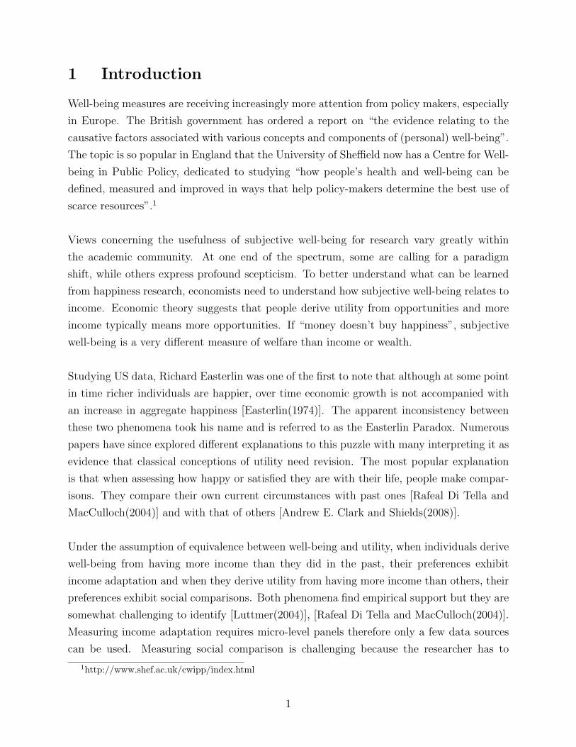
Happiness and Income Inequality

Jean-Benoıt G. Rousseau ∗†

Montreal, September 17, 2009

Abstract

This paper shows that the lack of growth in average well-being, despite substantial

GDP per capita growth, in the US is not a paradox. It can be explained by changes

in the income distribution and the concavity of the happiness function. Since 1975 in

the United-States practically all of the income gains that have accrued to households

have gone to the richest 20%; income inequality has increased significantly. During

that time, in the US, the happiness gap between the rich and the poor has widened

substantially; happiness has stagnated for the rich and fallen for the poor which is

interpreted has rising happiness inequality. This pattern of spreading well-being be-

tween the income groups is also observed in Europe. These phenomena reflect the fact

that although “money buys happiness”, the relationship between the two is concave.

Analysis suggests that the happiness function can be approximated by the log-linear

form and confirms that there is no satiation in the function. The cost of extra hap-

piness increases with an individual’s wealth. The paper also explores and rejects the

possibility that the paradox results from measurement error. Corrections for the slope

of the happiness function are estimated for taxes and the transitory nature.

JEL: B41, D12, D60, D63, I31

∗Post-Doc, Public Policy Group, CIRANO, Montreal, Canada†This research was funded in part by grants from the Social Sciences and Humanities Research Council of

Canada (SSHRC) and the Fond de Recherche sur la Societe et la Culture du Quebec (FQRSC). I am gratefulto Miles Kimball, Dan Silverman, Robert J. Willis, David Y. Albouy, Norbert Schwarz, Dan Simundza,Matias Busso, Andrew Goodman Bacon and Ron Alquist for their help. I should be held responsible forremaining errors.

1

1 Introduction

Well-being measures are receiving increasingly more attention from policy makers, especially

in Europe. The British government has ordered a report on “the evidence relating to the

causative factors associated with various concepts and components of (personal) well-being”.

The topic is so popular in England that the University of Sheffield now has a Centre for Well-

being in Public Policy, dedicated to studying “how people’s health and well-being can be

defined, measured and improved in ways that help policy-makers determine the best use of

scarce resources”.1

Views concerning the usefulness of subjective well-being for research vary greatly within

the academic community. At one end of the spectrum, some are calling for a paradigm

shift, while others express profound scepticism. To better understand what can be learned

from happiness research, economists need to understand how subjective well-being relates to

income. Economic theory suggests that people derive utility from opportunities and more

income typically means more opportunities. If “money doesn’t buy happiness”, subjective

well-being is a very different measure of welfare than income or wealth.

Studying US data, Richard Easterlin was one of the first to note that although at some point

in time richer individuals are happier, over time economic growth is not accompanied with

an increase in aggregate happiness [Easterlin(1974)]. The apparent inconsistency between

these two phenomena took his name and is referred to as the Easterlin Paradox. Numerous

papers have since explored different explanations to this puzzle with many interpreting it as

evidence that classical conceptions of utility need revision. The most popular explanation

is that when assessing how happy or satisfied they are with their life, people make compar-

isons. They compare their own current circumstances with past ones [Rafeal Di Tella and

MacCulloch(2004)] and with that of others [Andrew E. Clark and Shields(2008)].

Under the assumption of equivalence between well-being and utility, when individuals derive

well-being from having more income than they did in the past, their preferences exhibit

income adaptation and when they derive utility from having more income than others, their

preferences exhibit social comparisons. Both phenomena find empirical support but they are

somewhat challenging to identify [Luttmer(2004)], [Rafeal Di Tella and MacCulloch(2004)].

Measuring income adaptation requires micro-level panels therefore only a few data sources

can be used. Measuring social comparison is challenging because the researcher has to

1http://www.shef.ac.uk/cwipp/index.html

1

construct the reference point of comparison (neighbors, average GDP/capita, hypothetical

person, etc.). Furthermore, some of the expected empirical manifestations of these prefer-

ences, such as differences in cross and within country well-being-income gradients, are not

observed in the data [Stevenson and Wolfers(2008a)].

Interpreting the Easterlin paradox as evidence that peoples’ preferences exhibit income adap-

tation and social comparisons has led many to the conclusion that governments should stop

pursuing economic growth and make income taxes more progressive [Layard(2005)]. The

idea is that people adapt to growing incomes and that lowering income differences would

raise average happiness. When individuals compare themselves to one another, the extra

utility someone receives from having a high income comes at the expense of those who com-

pare themselves with him. The pursuit of individual wealth should thus be discouraged by

increasing tax rates at the top.

Within the happiness literature, much effort has been targeted at explaining the happiness-

income puzzle with the Easterlin paradox almost systematically the starting point of anal-

ysis [Andrew E. Clark and Shields(2008)], [Frey and Stutzer(2002)]. Recently Stevenson

and Wolfers presented evidence suggesting a positive relationship between GDP growth and

average well-being [Stevenson and Wolfers(2008a)]. More precisely, they found that the in-

come well-being gradient is the same within country, across country and over time. Their

findings, they say, “put to rest the claim that economic growth doesn’t lead to happiness

and (...) undermine the role played by relative income comparisons”.2 Although it varies in

strength, evidence that economic growth raises aggregate happiness can be found roughly

everywhere outside the US. The authors conclude that “the failure of happiness to rise in the

US remains a puzzling outlier”. Thus the question: “Why has economic growth not raised

average happiness in the US?”.

Relying solely on classical economic theory, this paper proposes an explanation of the lack of

serial correlation between economic growth and average happiness in the US. The interpre-

tation builds on the concavity of the happiness function and takes into account the evolution

of income inequality over the last few decades.3 When the data is disaggregated by income

group, happiness trends observed in the US and elsewhere are consistent with agents whose

happiness depends solely on their own income, and not on past income or the income of

2Most theories of comparisons suggest that the within country income-well-being gradient should besmaller than the across country GDP-average-well-being gradient.

3The expression “happiness function” is used to describe the relationship between subjective well-beingand income.

2

others.

1.1 A simple explanation of the Easterlin Paradox

The lack of growth in aggregate happiness despite the economic growth experienced in the

US is not necessarily a paradox. If, as the economy grows, inequality increases in such a way

that incomes fall for the poor, the pull on average happiness being exerted by the rich will

be offset by the drag exerted by the poor. Although the income gains of the rich are larger

in magnitude than the losses of the poor, average income is growing, the concavity of the

function is such that the effects on well-being are similar. Figure 1 illustrates this intuition.

This interpretation of the Easterlin paradox builds on the following three propositions.

Proposition 1. The happiness function is concave.

Proposition 2. Real income has risen for the rich and fallen for the poor.

Proposition 3. Happiness has risen for the rich and fallen for the poor.

The paper shows that each proposition finds empirical support and extends the discussion

about the importance of income equality in the conversion of economic growth into aggregate

happiness to other countries. The analysis starts with a formal estimation of the curvature

of the happiness function. The existence of a satiation point, or plateau, is assessed by

examining the relationship between well-being and income among the richest. This is done

to test the idea that the happiness-income puzzle reflects the fact that, after a certain point,

“money doesn’t buy happiness”. The paper explores the evolution of the distribution of

income and well-being in the US, revealing that real income has indeed fallen for the bottom

and second income quintiles. Subjective well-being has followed a pattern similar to income

in that the gap between the rich and poor has widened over the last four decades. The rising

income gap between individuals at the top of the income distribution and their poorer coun-

terparts over the last 35 years has parallelled an increasing happiness gap. Finally, analyses

are conducted with data from Europe to confirm the important role of income inequality in

the conversion of economic growth into aggregate well-being.

The second part of the paper explores the possibility that the Easterlin paradox is a result

of measurement error. The idea is that even though measured income has been rising, true

income may have remained flat, explaining the lack of growth in happiness. The slope of the

happiness function is estimated for corrections for taxes and the transitory nature of income.

3

The paper is organized as follows: Section 2 describes the data used for the analysis. Specific

descriptions of the subjective well-being and income measures are presented, along with an

explanation of the method used for converting the qualitative subjective well-being answers

to quantitative information . Section 3.1 presents an estimation of the degree of curvature

of the happiness function and tests for the existence of a satiation point the well-being. A

discussion of the evolution of the income distribution (3.2) and the rich-poor happiness gap

(3.3) in the US follows. Section 3.5 uses European data to assess whether patterns observed

in other countries confirm the importance of the concavity of the well-being function and

income inequality in the conversion of economic growth into general subjective well-being.

Section 4.1 investigates the effect of different corrections for the income variable. Finally,

Section 5 concludes.

2 Data

Four sources of data are used in this paper. The General Social Survey (GSS) is a repeated

micro-level cross section of about 1600 Americans covering the years from 1972 to 2006

(with some gaps). The Health and Retirement Study (HRS) is a bi-annual panel of roughly

22,000 retired Americans covering the years from 1992 to 2004. The Eurobarometer (EB) is

a repeated cross-section of anywhere between 450 and 4250 respondents (averaging at about

1600) from different European nations from 1974 to 2004. The same countries are sampled

annually with countries added over time. The German Socio Economic Panel (GSOEP) is

an annual panel of about 2750 German adults; it gathers detailed socioeconomic information

as well as a life satisfaction measure over a period ranging from 1984 to 2005.

2.1 Well-Being

Table 1 reports the questionnaire items used to measure subjective well-being in each of the

surveys. With the exception of the HRS, the items are somewhat similar. The HRS mea-

sures come from answers to a subset of questions from the Center for Epidemiologic Studies

of Depression (CES-D), aimed at measuring depressive symptoms. The questions ask “Now

think about the past week and the feelings you have experienced. Please tell me if each of

the following was true (Yes/No) for you much of the time this past week? Much of the time

during the past week you have felt - sad, happy, depressed and enjoyed life”.

When estimating the degree of curvature of the happiness function, simply converting the

4

qualitative answers into numbers would not be appropriate because the choice of scale could

affect the estimation.4 For that reason this paper turns to the method used by Stevenson

and Wolfers for aggregating well-being scores across groups [Stevenson and Wolfers(2008a)].

The idea is to use the coefficients from ordered probit regressions of subjective well-being

on group dummies (with no other controls) as the average well-being for that group. The

following makes the procedure explicit.

SWBit = β0 + Iit∆k + εit

The subscripts i and t denote individuals and time periods. SWBit is the subjective well-

being of the respondent. The variable Iit is a n × k matrix of binary group membership

indicators and ∆k is a k × 1 vector of coefficients. The coefficients, δ, are interpreted as

well-being indices that capture shifts in an underlying normally distributed latent well-being

variable. Unless otherwise specified, the ordered probits are estimated on the entire sample

(all years, countries, etc.). Depending on the grouping variables used, the procedure allows

for different levels of aggregation, i.e. ∆k can take different lengths.

δnt Country×year averages(k = t× j)

δjnt Income groups × countries × year averages (k = j × n× t)

For the curvature analysis, the groups are either the income categories in the survey or twenty

equally weighted bins (each with 5% of the income distribution) used as group dummies if

the income variable is continuous, as it is the case in the HRS and GSOEP,. These subjective

well-being indices are also employed to present the data graphically.

2.2 Income

Table 2 reports the wording of the questionnaire items used to collect the information about

the respondents’ income. The GSOEP and the HRS are the only two sources of data to have

non-categorical income measures. The GSS, the WVS and the EB rely on roughly 5 to 15

income categories per country-wave. For these surveys the income variable is converted into

a numerical figure by assigning the value that corresponds to the mid-point of the income

categories chosen by the respondent. The highest income bracket is converted by adding half

of the distance between the top and bottom bounds of the previous category to the lowest

bound of the top category.5 For most surveys, the income categories do not change annually

4For example, the GSS is usually coded according to: “Not too Happy”=1, “Pretty Happy”=2 and “VeryHappy”=3.

5For example, if the previous to last category is $45,000 to $55,000 and the top category is $55,001 andup, the numerical figure attributed to respondents that chose the top income category is $60,000.

5

year but do so relatively frequently, at least once every five years.

For the GSS, a net of tax income measure is obtained using the National Bureau of Economic

Research TAXSIM 8 software.6 The available criteria used for the tax simulation are the

year, the number of dependents, the marital status and the respondent’s nominal household

income.

GDP per capita and CPI, used to convert nominal into real figures, come from the World

Penn Tables [of Pennsilvanya(2007)] and the OECD web site [OECD(2007)].

3 Analysis

This section provides empirical evidence in support of Propositions 1, 2 and 3. The

analysis starts by exploring the properties of the well-being function. The evolution of the

income and happiness distribution in the US over the last forty years follows. European data

is then analyzed to investigate the role of income inequality in the conversion of economic

growth into well-being. Finally, formal estimations of the well-being income gradient are

reported for different corrections in the measurement of the income variable.

3.1 Proposition 1: The Happiness Function

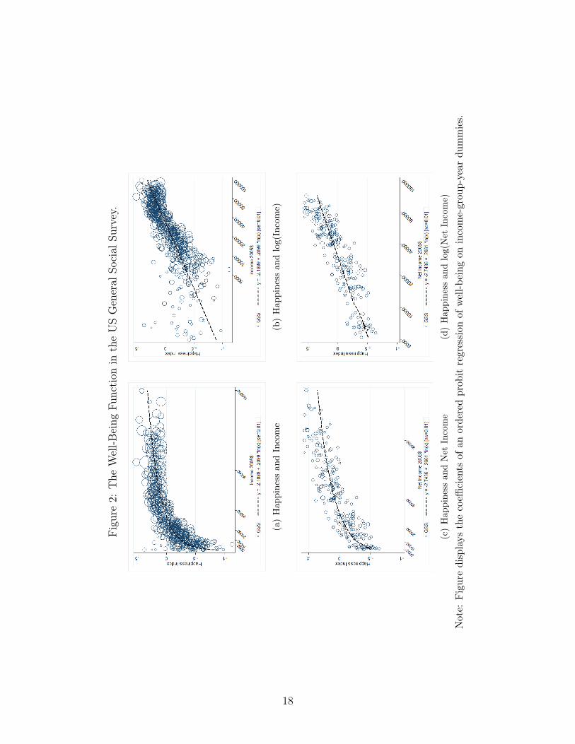
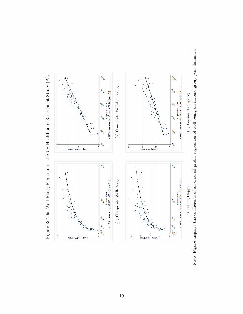
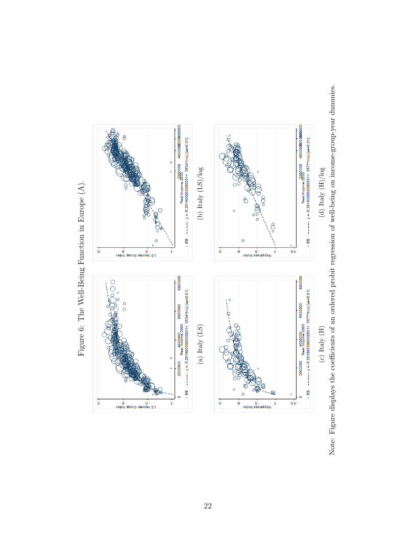
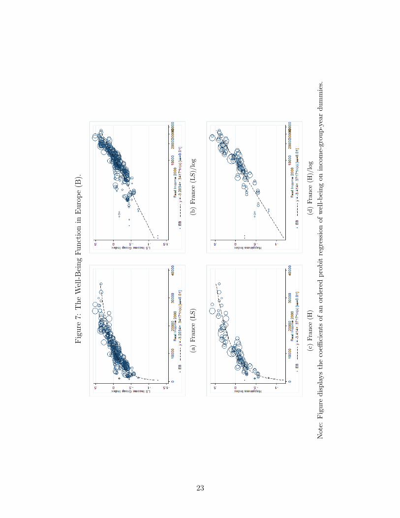
Figures 2 through 6 present cross-sections of real income and subjective well-being indices

for the US, Germany and other European countries. As explained earlier, the SWB indexes

come from country-specific ordered probit regressions of happiness on income-group-year

membership variables. The index is the coefficient on a respondent’s group.

The left hand side figures plot SWB and income on a normal scale and the right hand side

figures present SWB and income on a logarithmic scale. Every year for which the data was

collected is super-imposed, the x axis is in real figures. The dashed lines plot well-being

predicted by a linear regression of the well-being indices on the logarithm of income (no

controls). The shape of the well-being function is remarkably similar across countries. These

figures should rule out any doubt about the concavity of the well-being function. In every

country and for every well-being measure, the relationship between individual income and

well-being is clearly concave. Also, in the US, correcting for taxes (Figure 3c and 3d) elim-

inates what appears to be a group of very happy poor outliers visible on the raw income

6http://www.nber.org/ taxsim/taxsim-calc8/index.html

6

figure (3a and 3b).

To formalize the insight that emerges from visual inspection of the figures, the degree of

curvature of the well-being function is estimated through a Box-Cox transformation analysis.

The procedure estimates

SWBi = α + βg(yi) + εi where g(yi) = (yλi − 1)/λ

yi represent individual i income. The λ captures the degree of curvature of the function. A

λ greater than 1 implies a convex function. At exactly 1, the function is linear and for values

below 1 the function is increasingly concave. Finally, the function is of the logarithm form

when λ equals 0. Figure 8 plots g(y) for different λ on a linear and logarithmic scale. Notice

that when the underlying function is less concave than the logarithm, it appears convex

when plotted on a logarithm scale; the converse is also true.

The second column of Table 3 and Table 4 report country specific estimates of λ. The

estimates confirm the concavity of the well-being function regardless of the country and

subjective well-being measure. For the US the well-being function estimated with the GSS

data is less concave (λ = 0.5) than that estimated with the HRS data (around 0). This is

not due to the fact that income in the GSS does not account for taxes and transfers since

the degree of curvature estimated with net income actually suggests a less concave function

(λ = 0.6). When income is measured directly (HRS), as opposed to categorically, the degree

of curvature of the happiness function estimated in the US is close to zero, the log-linear form.

In Europe, the degree of concavity of the well-being function appears to vary a great deal

across countries (second and third column). However, as discussed earlier, this could be due

to differences in tax systems. Estimates of the degree of curvature of the life satisfaction

function range from 0.1 (Greece) to 1.3 (Ireland). In all but one country (Belgium), esti-

mates of the degree of curvature of the happiness function are lower (weakly), implying a

more concave function, and range from -0.2 (England) to 0.4 (Germany).

The relationship between income and life satisfaction is less concave than the relationship

between income and happiness. Differently put, the marginal happiness of a dollar diminishes

at a faster rate than the marginal life satisfaction of a dollar. One possible explanation is

that the life satisfaction question more explicitly asks respondents to make comparisons when

assessing their well-being. Indeed, when respondents focus on other peoples’ circumstances;

7

extra income has an important effect on well-being even at high levels. For most functional

forms, an increase in income improves an individual’s relative position regardless of where

he/she is along the income distribution (unless at the top). More generally, the channels

linking income and life satisfaction might be different than the channels linking income

and happiness. These different properties point to the fact that failing to make a distinction

between the two measures may be a mistake. For example, one should be wary of comparisons

between a within-country happiness gradient and a across-country life satisfaction gradient.

3.1.1 Satiation

Newspaper articles often suggest that the lack of growth in average happiness is due to the

existence of a satiation point in the happiness function, i.e. a level of income above which

additional income does not affect happiness [Begley()]. To explore this possibility the effect

of income among the very rich is investigated. If the happiness function exhibits satiation,

money should not buy happiness for this subpopulation.

The third, fourth and fifth columns of Table 3 and Table 5 report the smallest top income

decile within which income has a statistically significant positive effect on well-being. The ta-

bles report the estimated coefficient from ordered probits and the corresponding full-sample

estimate. For instance, in the GSS, when raw income is used, the smallest top income group

for which income increases happiness is 10%. At 0.393, the income coefficient is actually

higher within that group than among the whole population, 0.239. Using net income does

not affect these results. The smallest top groups in the HRS are somewhat larger and the

effect of income is smaller in those groups. Looking at the figures (2 and 3) reveals that

a large number of middle income earners report being “highly happy” for three of the four

HRS well-being measures . Additionally, out of all four, “Feeling depressed” is the well-being

indicator that behaves most like the GSS happiness question. The results are very similar

in Europe, where income raises well-being even among the top 10% richest These results are

shown in Table 5.

The well-being function is clearly concave and there is no evidence of satiation as the well-

being function is positively sloped even among top earners. Proposition 1 is confirmed.

Furthermore, using a log-linear function to capture the concavity of the relationship between

individual well-being and income, as is the norm in the field, is a valid choice since it

corresponds to the degree of parametrically estimated concavity. This specific form implies

that proportional income gains bring the same well-being gain regardless of one’s position

8

on the income distribution. Money buys happiness but, it gets more expensive as people get

richer.

3.2 Proposition 2: Income Inequality

Panel (a) of Figure 9 shows the evolution of real income for each quintile of the US General

Social Survey. Income inequality has grown among the GSS respondents over the last four

decades. Real income for the bottom and second quintiles has decreased by an average of

0.58% and 0.55% a year respectively. Real income for the third, fourth and top quintiles has

increased by an average of 0.15%, 0.79% and 0.90% a year respectively. The gap between

the 1st and 5th quintile has thus grown by about 1.5% per year. While the average income

of the top quintile was about 9 times larger than that of the bottom’s in 1973 it was close to

10.5 times larger by the end of 2006 . The income patterns in the GSS support Proposition

2. Furthermore, because it is conducted with income measured with categorical questions,

the analysis most likely underestimates the magnitude of the rise in income inequality.

3.3 Proposition 3: The Happiness Gap

Panel (b) of Figure 9 reports the happiness for each quintile of the GSS since 1973. Happi-

ness has polarized over the years, decreasing for the bottom quintiles and stagnating for the

top quintiles. Figure 10 presents the evolution of the percentage of respondents answering

“Very Happy”, “Pretty Happy” and “Not too Happy” for each income group. The figure

shows that the proportion of the poorest respondents reporting to be “Very Happy” dropped

for every income quintile over the last four decades. The proportion of richest respondent

reporting to be “Unhappy” has also dropped over the same period. Interestingly, the fre-

quency of “Very Happy” answers has dropped while the frequency of “Happy” has risen for

every income group since the mid-seventies. The happiness gap between the rich and poor

has widened because the switch from “Very Happy” to “Happy” has been more drastic for

the poorer income groups.

To get a sense of the magnitude of the widening of the happiness gap, Table 6 reports

estimates from four different specification of the following ordered probit:

SWBit = β0 + βPPoorit + βMMidit + βXControlsit

+βPT (Poor × Time) + βMT (Mid× Time) + βRT (Rich× Time) + εit

where Poorit, Midit and Richit are mutually exclusive group dummies representing the mem-

9

bership of respondent i to the bottom, middle three or top income quintiles in period t. βP

and βM capture the difference in happiness between the corresponding group and the rich

in 1973. The coefficients on the (Group × Time) variables, βPT , βMT and βRT reflect the

average annual change in happiness for each group. Controlsit include the respondent’s age,

gender, ethnicity, marital status and education.

To help with the interpretation, column (4) is discussed in detail; this specification includes

the sociodemographic controls. As captured by βP , the happiness gap between the rich and

poor in 1973 was 60% of one standard deviation. This difference grew by 0.44% every year

(βPT ) to reach 74.5% by the end of 2006 (βPT × 33 years). The happiness gap between the

top and bottom income quintile has grown by 14.5% of one standard deviation over that

period.7 Said differently, the happiness difference between the bottom 20% poorest and the

top 20% richest is 25% larger in 2003 than it was in 1975. During the same period, the

income gap between these groups rose by 0.4 standard deviations.

The estimated happiness gap between the middle and rich income group(βM) was 21.73%

of one standard deviation in 1973. It grew by 0.39% (βMT ) every year to reach 34.6% of a

standard deviation in 2006 (βMT × 33 years), a 12.9% increase. Notice that the gap between

the middle and bottom quintiles remained roughly constant over that period since the well-

being of both groups decreased at a similar rate.

The widening of the happiness gap is confirmed. It is not attributable to changes in the

composition of the quintiles since the exclusion of controls does not affect the results. In the

US, happiness has fallen for the poor and middle income groups and stagnated for the rich

(Proposition 3 is confirmed). Stevenson and Wolfers discuss the fall in overall variance

in happiness since the mid-seventies and interpret this decline as a decline in happiness

inequality [Stevenson and Wolfers(2008b)]. In light of the facts that the happiness of the

poor has fallen and the gap between the rich and poor has widened this interpretation

appears misleading. Indeed, both in relative and absolute terms, poor people are less happy

today than they were in the seventies.

3.4 The Easterlin Paradox Revisited

The idea that the happiness income puzzle can be explained solely by the concavity of the

happiness function and the evolution of incomes finds support in the data. 1) The happiness

7The ordered probit normalizes the standard deviation to one.

10

function is concave. 2) Income inequality has increased since the mid seventies and real

income has fallen for the poorest two quintiles. 3) Happiness tracks income changes along

a concave function, well-being has stagnated for the rich and dropped for the poor. The

following subsection investigates the role of income inequality in the conversion of economic

growth into aggregate well-being in other countries to further validate this reading of the

happiness income puzzle.

3.5 The Happiness-Income Puzzle in Europe

Table 8 and 9 report estimates of the rich poor well-being gap and its evolution for each

country. The bottom rows of the table report the evolution of the well-being gap over time.

GDP per capita increased in all countries during the time of the survey. These regressions

are country specific and include year dummies as well as a set of controls for age, ethnicity,

gender, marital status and education. The interpretation of the coefficients is the same as

that of Table 6.

In countries where income inequality has either fallen or remained constant, average life sat-

isfaction has risen on par with GDP per capita. This is the case in France, Germany, Italy,

Luxembourg, Denmark, and Spain. In Holland and Great Britain, average life satisfaction

has risen despite rising income inequality. This is not inconsistent with the interpretation of

the Easterlin paradox put forward in this paper.8 Portugal displays patterns similar to the

US. In both countries, aggregate well-being stagnated (failed) despite a growing economy.

In that sense, the Easterlin paradox is not exclusively an American phenomenon.

In all but one country (Belgium), economic growth was accompanied by an (weak) increase

in the rich-poor well-being gap. This should be regarded as a stylized characteristic of the

relationship between subjective well-being and income over time.

Table 10 reports estimates of country-level life satisfaction regressions. Column (1) estimates

the effect of the logarithm of GDP per capita on aggregate life satisfaction. The gradient

is positive and significant at 0.183. The second specification (2) looks at the effect of the

average logarithm of income which captures changes in the income distribution not captured

by average income. The gradient for this estimation is roughly half of the ln(GDP) coefficient

8As long as the whole income distribution benefits from the economic growth (i.e. real incomes do notfall for the poor) average well-being will rise despite increasing income inequality. Furthermore, even if realincomes fall for the poor, average well-being will rise if the well-being gains of the rich is larger than thewell-being loses of the poor.

11

at 0.096. However, when the estimation includes both variables (Column 3), only the average

log-income remains significantly linked to aggregate well-being, confirming the role of income

inequality in the conversion of economic growth into aggregate well-being. Overall, the

patterns in Europe are consistent with the notion that aggregate well-being is driven by

individual income.

4 Discussion

4.1 Taxes and Permanent Income

Another explanation of the happiness-income puzzle is that the lack of growth in average

happiness as a function of income reflects the fact that income is improperly measured. The

idea is that although measured income has risen substantially since the seventies, true in-

come has not. This section looks at whether correcting for taxes and the transitory nature

of income affects the relationship between income and subjective well-being.

Table 7 reports estimates from ordered probit regressions of subjective well-being on differ-

ent income measures. The estimation uses data from the GSS and from the GSOEP. Note

that while the GSS well-being measure asks about the respondent’s happiness the GSOEP

measure asks about life satisfaction. The log-linear form is assumed for these estimations.

Column (1) reports the estimated happiness-income gradient from an ordered probit of well-

being on raw income in the US. Column (2) presents the same specification using net income

computed with TAXSIM8. Both specifications include year dummies and controls for age,

marital status, gender and race. Under the assumption that happiness, like utility, depends

on disposable income, one would expect net income to have a larger effect on well-being. This

is indeed the case; the coefficient is 0.15 for raw income and 0.16 for net income. Although

the coefficients are statistically different the difference is minimal. Column (3) reports the

same coefficient using data from Germany, with life satisfaction as the well-being variable.

The income well-being gradient is higher in this case but since both the sample and well-

being measure are different across the countries, discussion will be limited to within country

comparisons. Column (4) presents the estimate obtained with a fixed-effect model. This

model does not affect the gradient substantially.

Column (5) uses lagged income to proxy for permanent income to test the hypothesis that

well-being, like utility, depends not on transitory income but permanent income. The argu-

12

ment as to why lagged income is a proper instrument for permanent income is detailed in the

Appendix. Succinctly put, the only part of lagged income that is related to contemporaneous

well-being is the permanent part, this is not the case for contemporaneous income. This cor-

rection actually lowers the well-being-income gradient (0.221). The fact that unlike utility,

well-being depends on transitory income, could be interpreted as evidence that well-being

does not measure utility. Overall, the Easterlin paradox does not appear to be a result of

mismeasurement of income.

4.2 Income Adaptation and Social Comparison

The interpretation of the Easterlin paradox presented in this paper does not rule out the

possibility that individual preferences exhibit income adaptation or social comparison. It

does however call into question the stylized facts that have motivated most discussions of

these phenomena in happiness research as well as the notion that aggregate happiness data

is informative of individual preferences. There is evidence that individuals compare their

circumstances with that of others and get accustomed to changes in their lives [Frey and

Stutzer(2002)]. Whether these phenomena have an economically important effect at the

macroeconomic level is unclear.

Research on hedonic adaptation suggests that people adapt to new circumstances very

rapidly. Kimball, Ohtake, and Tsutsui find that the type of adaptation described by psy-

chologists takes place over very short periods of time [Miles Kimball and Tsutsui(2006)].

Kimball and Silverman find, for example, that widows adapt to the loss of their partner in

about nine months [Kimball and Silverman(2008)]. The type of adaptation described by

psychologists and studied by the authors does not seem to be the mechanism at work in the

behavior of long run happiness.

Research on social comparison suggests that people compare themselves to people who are

geographically close to them [Barrington-Leigh and Helliwell(2008)]. One implication is

that the well-being income gradient should be smaller for cross-country than for within-

country regressions. When individuals derive utility from comparisons with people living in

their own country, regressions are driven not by between-country variations but by within-

country variations. In fact, if agents only care about where they rank in their country, there

should be no positive association between a nation’s GDP per capita and the average level

of subjective well-being. Stevenson and Wolfers could not reject the hypothesis that the

within and between-country gradients are equal [Stevenson and Wolfers(2008a)]. This paper

13

investigated the possibility that this is due to errors in the measurement of income and found

that it is not the case.

5 Conclusion

This paper presents the Easterlin paradox under a new light. It argues that the assump-

tion of equivalence between happiness and utility does not necessarily lead to the conclusion

that peoples’ preferences are different than what standard notions of utility suggest. Like

the utility function described in introductory economics courses, the relationship between

income and subjective well-being is concave. Whether this should be interpreted as evidence

that subjective well-being captures utility is an open question.

The lack of growth in aggregate happiness despite massive economic growth reflects the fact

that, over the last few decades, income gains have accrued to the top income earners to such

a disproportionate extent that income has fallen for the poor. Over the last thirty-five years

the happiness gap between the rich and the poor has widened in pair with income inequality.

Regardless of the reason given, happiness is nowadays more a commodity of rich people than

it was thirty-five years ago. Analysis of patterns in European countries confirm the crucial

role of income inequality in the conversion of economic growth into aggregate well-being.

The increased well-being gap between the rich and poor has widened in other developed

countries. It appears that this fact should receive additional attention and be consider as

a stylized fact of the relationship between income and happiness. Correcting for taxes has

little effect on the estimated slope of the happiness function and using permanent rather

than transitory income surprisingly lowers the gradient.

The conclusions reached in this paper extend naturally to those reached in other fields of

economics: income equality matters. Whether it is because people compare themselves to

each other or because the happiness function is concave, the income distribution affects how

resources are converted into well-being. Raising national happiness with policies aimed at

accelerating the economic development of a country is not ineffective if the expansion bene-

fits the entire income distribution.

On a theoretical level, economists understand how utility relates to income. Bridging the

gap between theory and practice can be a difficult task as utility per se is not measurable.

Economists have partly resolved this issue by studying peoples’ choices but choices are only

informative of preferences; they do not allow for comparisons across individuals. For many,

14

this is precisely the appeal of happiness data. This paper attempts to inform the debate

about the relationship between happiness and utility by exploring an alternative interpreta-

tion of the stylized facts of happiness research.

More work is needed before economists can clearly understand the relationship between

subjective well-being and utility. Few studies have investigated the production of happiness.

An agent’s time allocation is paramount to his welfare. Furthermore, knowing that time is

an important input for happiness opens the door to a promising area of research.

15

APPENDIX

Permanent IncomeLagged income (Yt−1) can be used as a proxy for permanent income (Y P

t ). Under thepermanent income hypothesis, observed income (Yt) has a permanent (Y P

t ) and transitory(Y T

t ) component. A consumers’ utility depends on permanent income.

Yt = Y Tt + Y P

t

Yt−1 = Y Tt−1 + Y P

t−1

The correlation between Yt and Ht does not isolate the effect of permanent income onhappiness. However, if income follows a random walk, the only part of lagged income relatedto contemporaneous well-being is the permanent part, it can thus serve as a proxy for Y P

t .

Cov(Y Pt−1, Y

Pt ) > 0, Cov(Y T

t , YPt ) = 0, Cov(Y T

t−1, YPt−1) = 0 and Cov(Y T

t , YTt−1) = 0

Cov(Yt−1, Ht)

Cov(Yt−1, Yt)'

Cov(Y Pt−1, Ht)

Cov(Y Pt−1, Y

Pt )

16

Figure 1: Economic Growth and Falling Average Happiness.

Note: The Figure illustrates the happiness of two individuals, with the same concave utility function,who’s happiness changes across two periods as a result of changes in their income. The resultis an overall increase in average income and a drop in average happiness.

17

Fig

ure

2:T

he

Wel

l-B

eing

Funct

ion

inth

eU

SG

ener

alSoci

alSurv

ey.

(a)

Hap

pine

ssan

dIn

com

e(b

)H

appi

ness

and

log(

Inco

me)

(c)

Hap

pine

ssan

dN

etIn

com

e(d

)H

appi

ness

and

log(

Net

Inco

me)

Not

e:F

igur

edi

spla

ysth

eco

effici

ents

ofan

orde

red

prob

itre

gres

sion

ofw

ell-

bein

gon

inco

me-

grou

p-ye

ardu

mm

ies.

18

Fig

ure

3:T

he

Wel

l-B

eing

Funct

ion

inth

eU

SH

ealt

han

dR

etir

emen

tStu

dy

(A).

(a)

Com

posi

teW

ell-

Bei

ng(b

)C

ompo

site

Wel

l-B

eing

/log

(c)

Feel

ing

Hap

py(d

)Fe

elin

gH

appy

/log

Not

e:F

igur

edi

spla

ysth

eco

effici

ents

ofan

orde

red

prob

itre

gres

sion

ofw

ell-

bein

gon

inco

me-

grou

p-ye

ardu

mm

ies.

19

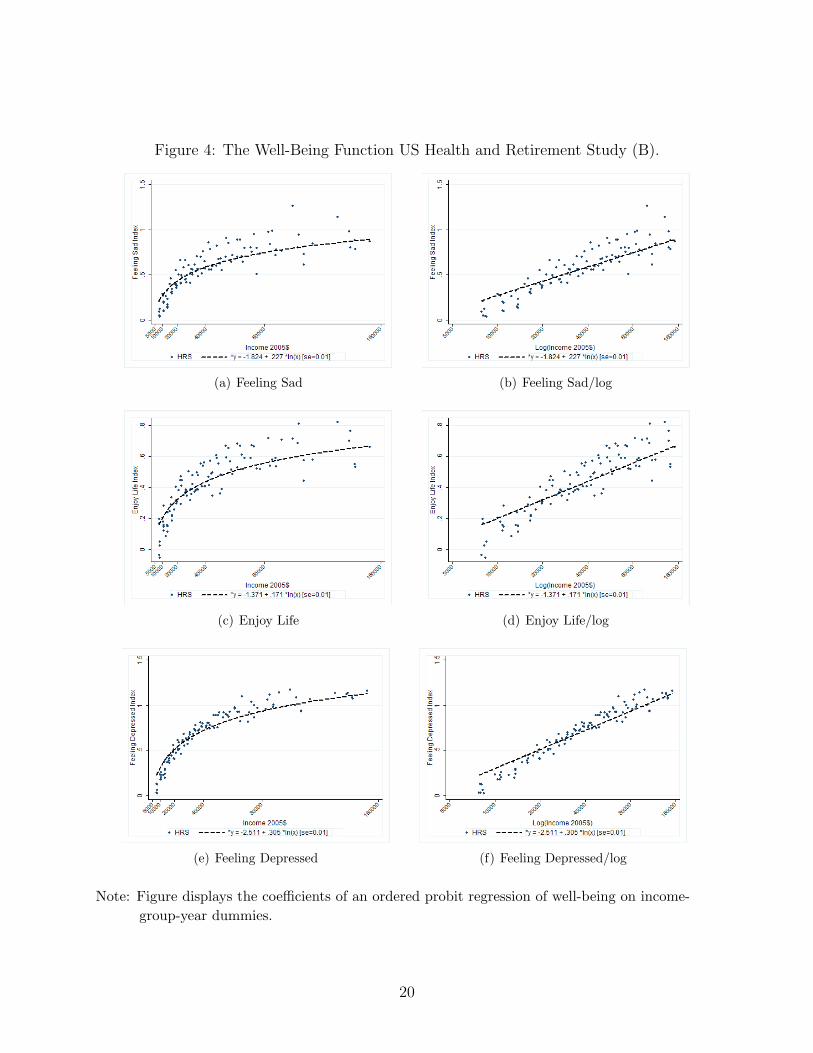
Figure 4: The Well-Being Function US Health and Retirement Study (B).

(a) Feeling Sad (b) Feeling Sad/log

(c) Enjoy Life (d) Enjoy Life/log

(e) Feeling Depressed (f) Feeling Depressed/log

Note: Figure displays the coefficients of an ordered probit regression of well-being on income-group-year dummies.

20

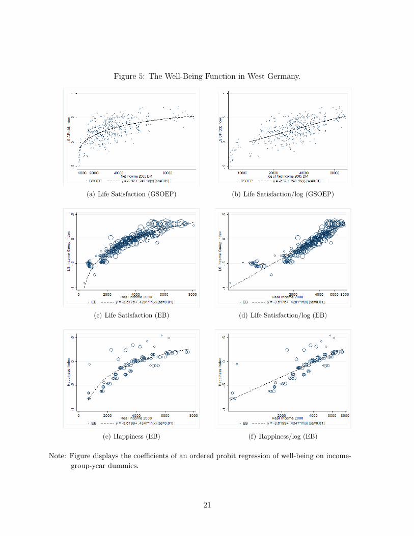
Figure 5: The Well-Being Function in West Germany.

(a) Life Satisfaction (GSOEP) (b) Life Satisfaction/log (GSOEP)

(c) Life Satisfaction (EB) (d) Life Satisfaction/log (EB)

(e) Happiness (EB) (f) Happiness/log (EB)

Note: Figure displays the coefficients of an ordered probit regression of well-being on income-group-year dummies.

21

Fig

ure

6:T

he

Wel

l-B

eing

Funct

ion

inE

uro

pe

(A).

(a)

Ital

y(L

S)(b

)It

aly

(LS)

/log

(c)

Ital

y(H

)(d

)It

aly

(H)/

log

Not

e:F

igur

edi

spla

ysth

eco

effici

ents

ofan

orde

red

prob

itre

gres

sion

ofw

ell-

bein

gon

inco

me-

grou

p-ye

ardu

mm

ies.

22

Fig

ure

7:T

he

Wel

l-B

eing

Funct

ion

inE

uro

pe

(B).

(a)

Fran

ce(L

S)(b

)Fr

ance

(LS)

/log

(c)

Fran

ce(H

)(d

)Fr

ance

(H)/

log

Not

e:F

igur

edi

spla

ysth

eco

effici

ents

ofan

orde

red

prob

itre

gres

sion

ofw

ell-

bein

gon

inco

me-

grou

p-ye

ardu

mm

ies.

23

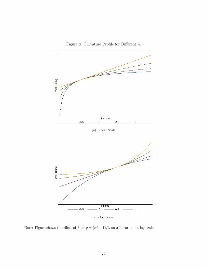
Figure 8: Curvature Profile for Different λ.

(a) Linear Scale

(b) log Scale

Note: Figure shows the effect of λ on y = (xλ − 1)/λ on a linear and a log scale.

24

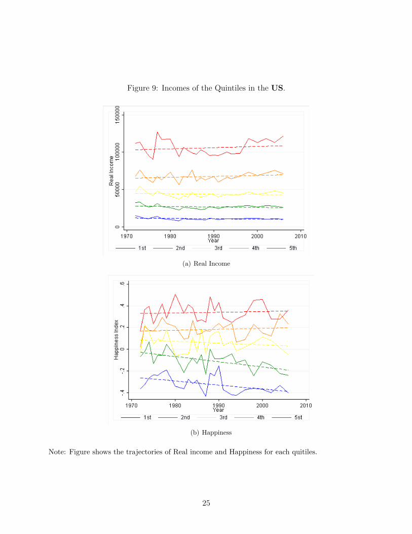
Figure 9: Incomes of the Quintiles in the US.

(a) Real Income

(b) Happiness

Note: Figure shows the trajectories of Real income and Happiness for each quitiles.

25

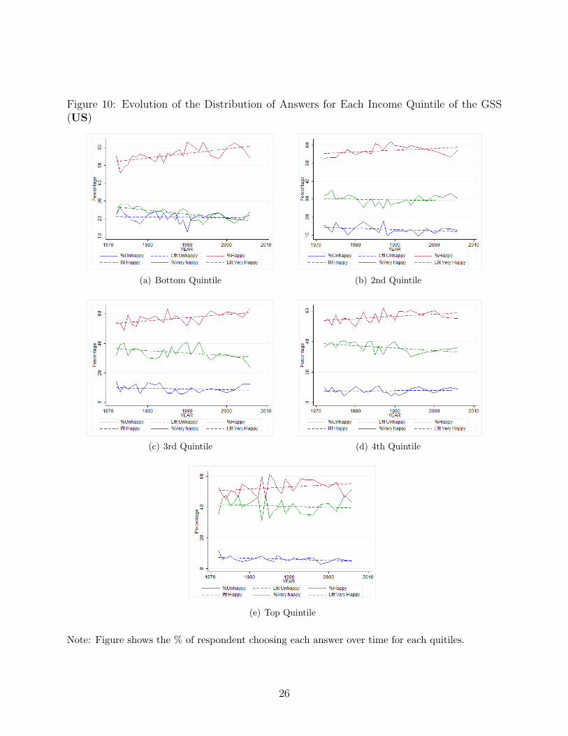
Figure 10: Evolution of the Distribution of Answers for Each Income Quintile of the GSS(US)

(a) Bottom Quintile (b) 2nd Quintile

(c) 3rd Quintile (d) 4th Quintile

(e) Top Quintile

Note: Figure shows the % of respondent choosing each answer over time for each quitiles.

26

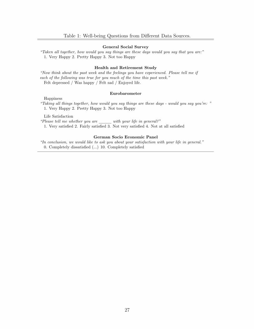
Table 1: Well-being Questions from Different Data Sources.

General Social Survey“Taken all together, how would you say things are these days would you say that you are:”

1. Very Happy 2. Pretty Happy 3. Not too Happy

Health and Retirement Study“Now think about the past week and the feelings you have experienced. Please tell me ifeach of the following was true for you much of the time this past week.”

Felt depressed / Was happy / Felt sad / Enjoyed life.

EurobarometerHappiness

“Taking all things together, how would you say things are these days - would you say you’re: ”1. Very Happy 2. Pretty Happy 3. Not too Happy

Life Satisfaction“Please tell me whether you are with your life in general?”

1. Very satisfied 2. Fairly satisfied 3. Not very satisfied 4. Not at all satisfied

German Socio Economic Panel“In conclusion, we would like to ask you about your satisfaction with your life in general.”

0. Completely dissatisfied (...) 10. Completely satisfied

27

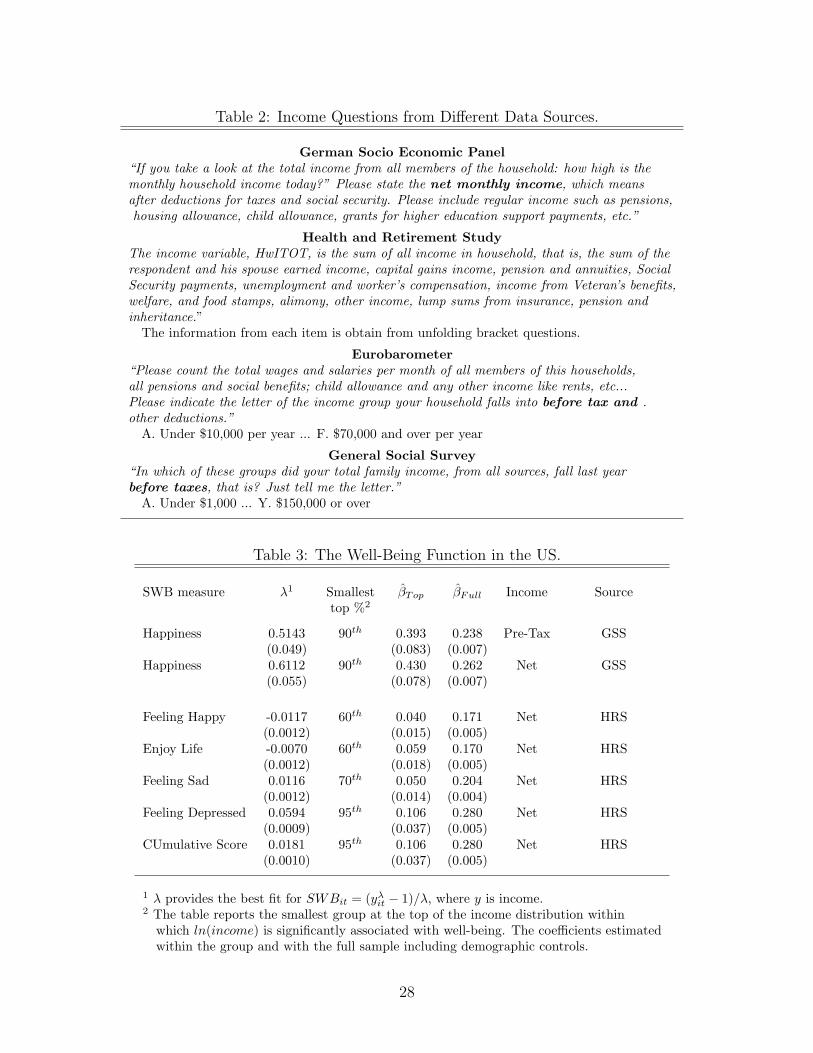
Table 2: Income Questions from Different Data Sources.

German Socio Economic Panel“If you take a look at the total income from all members of the household: how high is themonthly household income today?” Please state the net monthly income, which meansafter deductions for taxes and social security. Please include regular income such as pensions,housing allowance, child allowance, grants for higher education support payments, etc.”

Health and Retirement StudyThe income variable, HwITOT, is the sum of all income in household, that is, the sum of therespondent and his spouse earned income, capital gains income, pension and annuities, SocialSecurity payments, unemployment and worker’s compensation, income from Veteran’s benefits,welfare, and food stamps, alimony, other income, lump sums from insurance, pension andinheritance.”

The information from each item is obtain from unfolding bracket questions.

Eurobarometer“Please count the total wages and salaries per month of all members of this households,all pensions and social benefits; child allowance and any other income like rents, etc...Please indicate the letter of the income group your household falls into before tax and .other deductions.”

A. Under $10,000 per year ... F. $70,000 and over per year

General Social Survey“In which of these groups did your total family income, from all sources, fall last yearbefore taxes, that is? Just tell me the letter.”

A. Under $1,000 ... Y. $150,000 or over

Table 3: The Well-Being Function in the US.

SWB measure λ1 Smallest βTop βFull Income Sourcetop %2

Happiness 0.5143 90th 0.393 0.238 Pre-Tax GSS(0.049) (0.083) (0.007)

Happiness 0.6112 90th 0.430 0.262 Net GSS(0.055) (0.078) (0.007)

Feeling Happy -0.0117 60th 0.040 0.171 Net HRS(0.0012) (0.015) (0.005)

Enjoy Life -0.0070 60th 0.059 0.170 Net HRS(0.0012) (0.018) (0.005)

Feeling Sad 0.0116 70th 0.050 0.204 Net HRS(0.0012) (0.014) (0.004)

Feeling Depressed 0.0594 95th 0.106 0.280 Net HRS(0.0009) (0.037) (0.005)

CUmulative Score 0.0181 95th 0.106 0.280 Net HRS(0.0010) (0.037) (0.005)

1 λ provides the best fit for SWBit = (yλit − 1)/λ, where y is income.2 The table reports the smallest group at the top of the income distribution within

which ln(income) is significantly associated with well-being. The coefficients estimatedwithin the group and with the full sample including demographic controls.

28

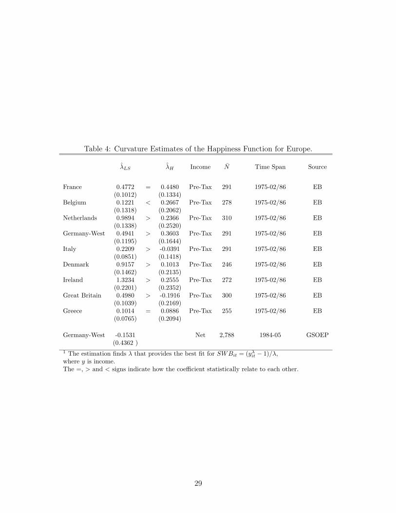
Table 4: Curvature Estimates of the Happiness Function for Europe.

λLS λH Income N Time Span Source

France 0.4772 = 0.4480 Pre-Tax 291 1975-02/86 EB(0.1012) (0.1334)

Belgium 0.1221 < 0.2667 Pre-Tax 278 1975-02/86 EB(0.1318) (0.2062)

Netherlands 0.9894 > 0.2366 Pre-Tax 310 1975-02/86 EB(0.1338) (0.2520)

Germany-West 0.4941 > 0.3603 Pre-Tax 291 1975-02/86 EB(0.1195) (0.1644)

Italy 0.2209 > -0.0391 Pre-Tax 291 1975-02/86 EB(0.0851) (0.1418)

Denmark 0.9157 > 0.1013 Pre-Tax 246 1975-02/86 EB(0.1462) (0.2135)

Ireland 1.3234 > 0.2555 Pre-Tax 272 1975-02/86 EB(0.2201) (0.2352)

Great Britain 0.4980 > -0.1916 Pre-Tax 300 1975-02/86 EB(0.1039) (0.2169)

Greece 0.1014 = 0.0886 Pre-Tax 255 1975-02/86 EB(0.0765) (0.2094)

Germany-West -0.1531 Net 2,788 1984-05 GSOEP(0.4362 )

1 The estimation finds λ that provides the best fit for SWBit = (yλit − 1)/λ,where y is income.The =, > and < signs indicate how the coefficient statistically relate to each other.

29

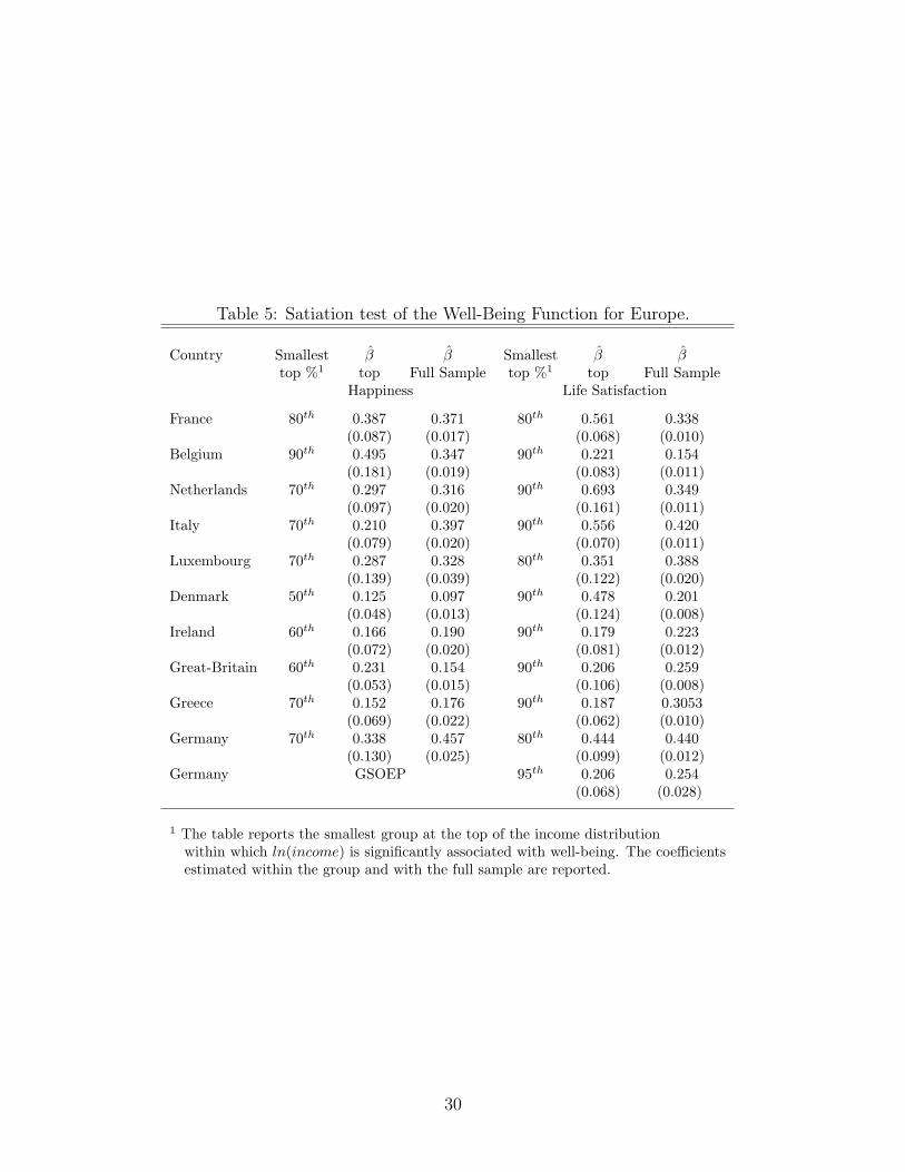
Table 5: Satiation test of the Well-Being Function for Europe.

Country Smallest β β Smallest β βtop %1 top Full Sample top %1 top Full Sample

Happiness Life Satisfaction

France 80th 0.387 0.371 80th 0.561 0.338(0.087) (0.017) (0.068) (0.010)

Belgium 90th 0.495 0.347 90th 0.221 0.154(0.181) (0.019) (0.083) (0.011)

Netherlands 70th 0.297 0.316 90th 0.693 0.349(0.097) (0.020) (0.161) (0.011)

Italy 70th 0.210 0.397 90th 0.556 0.420(0.079) (0.020) (0.070) (0.011)

Luxembourg 70th 0.287 0.328 80th 0.351 0.388(0.139) (0.039) (0.122) (0.020)

Denmark 50th 0.125 0.097 90th 0.478 0.201(0.048) (0.013) (0.124) (0.008)

Ireland 60th 0.166 0.190 90th 0.179 0.223(0.072) (0.020) (0.081) (0.012)

Great-Britain 60th 0.231 0.154 90th 0.206 0.259(0.053) (0.015) (0.106) (0.008)

Greece 70th 0.152 0.176 90th 0.187 0.3053(0.069) (0.022) (0.062) (0.010)

Germany 70th 0.338 0.457 80th 0.444 0.440(0.130) (0.025) (0.099) (0.012)

Germany GSOEP 95th 0.206 0.254(0.068) (0.028)

1 The table reports the smallest group at the top of the income distributionwithin which ln(income) is significantly associated with well-being. The coefficientsestimated within the group and with the full sample are reported.

30

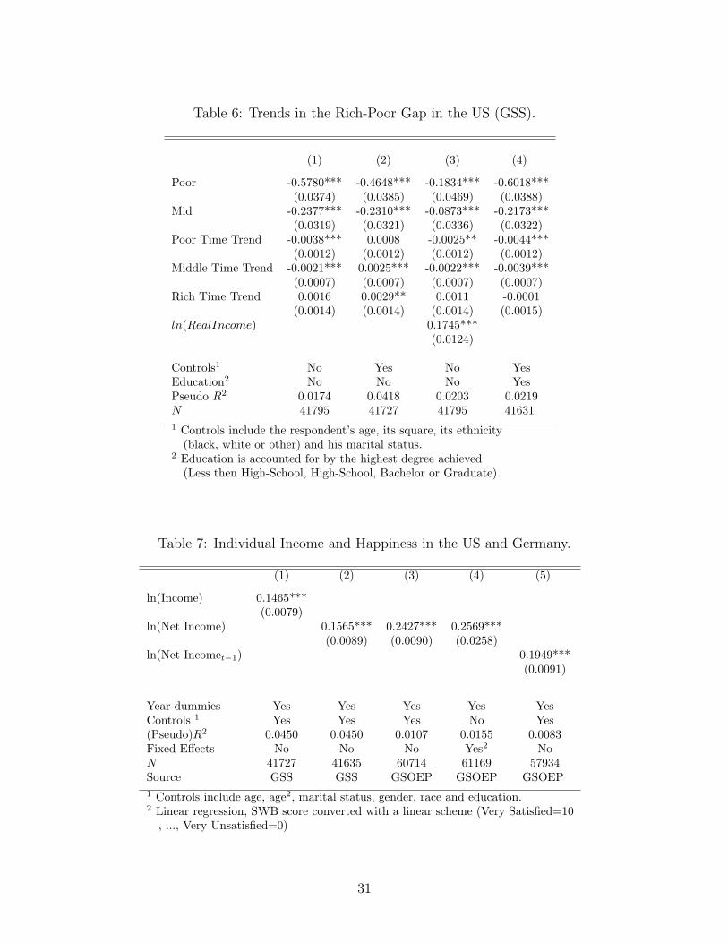
Table 6: Trends in the Rich-Poor Gap in the US (GSS).

(1) (2) (3) (4)

Poor -0.5780*** -0.4648*** -0.1834*** -0.6018***(0.0374) (0.0385) (0.0469) (0.0388)

Mid -0.2377*** -0.2310*** -0.0873*** -0.2173***(0.0319) (0.0321) (0.0336) (0.0322)

Poor Time Trend -0.0038*** 0.0008 -0.0025** -0.0044***(0.0012) (0.0012) (0.0012) (0.0012)

Middle Time Trend -0.0021*** 0.0025*** -0.0022*** -0.0039***(0.0007) (0.0007) (0.0007) (0.0007)

Rich Time Trend 0.0016 0.0029** 0.0011 -0.0001(0.0014) (0.0014) (0.0014) (0.0015)

ln(RealIncome) 0.1745***(0.0124)

Controls1 No Yes No YesEducation2 No No No YesPseudo R2 0.0174 0.0418 0.0203 0.0219N 41795 41727 41795 416311 Controls include the respondent’s age, its square, its ethnicity

(black, white or other) and his marital status.2 Education is accounted for by the highest degree achieved

(Less then High-School, High-School, Bachelor or Graduate).

Table 7: Individual Income and Happiness in the US and Germany.

(1) (2) (3) (4) (5)

ln(Income) 0.1465***(0.0079)

ln(Net Income) 0.1565*** 0.2427*** 0.2569***(0.0089) (0.0090) (0.0258)

ln(Net Incomet−1) 0.1949***(0.0091)

Year dummies Yes Yes Yes Yes YesControls 1 Yes Yes Yes No Yes(Pseudo)R2 0.0450 0.0450 0.0107 0.0155 0.0083Fixed Effects No No No Yes2 NoN 41727 41635 60714 61169 57934Source GSS GSS GSOEP GSOEP GSOEP1 Controls include age, age2, marital status, gender, race and education.2 Linear regression, SWB score converted with a linear scheme (Very Satisfied=10

, ..., Very Unsatisfied=0)

31

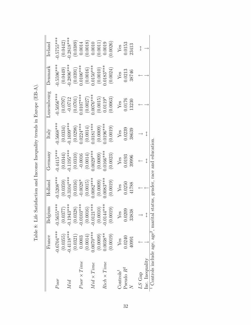
Tab

le8:

Lif

eSat

isfa

ctio

nan

dIn

com

eIn

equal

ity

tren

ds

inE

uro

pe

(EB

-A).

Fra

nce

Bel

gium

Hol

land

Ger

man

yIt

aly

Luxem

bou

rgD

enm

ark

Irel

and

Poor

-0.6

704*

**-0

.565

5***

-0.5

208*

**-0

.441

5***

-0.5

668*

**-0

.505

6***

-0.5

596*

**-0

.575

5***

(0.0

355)

(0.0

377)

(0.0

359)

(0.0

344)

(0.0

334)

(0.0

797)

(0.0

449)

(0.0

442)

Mid

-0.4

118*

**-0

.194

3***

-0.3

104*

**-0

.119

5***

-0.1

699*

**-0

.071

2-0

.289

6***

-0.2

818*

**(0

.032

1)(0

.032

8)(0

.031

6)(0

.031

0)(0

.029

8)(0

.070

1)(0

.039

1)(0

.038

9)Poor×Time

0.00

03-0

.010

3***

-0.0

028*

-0.0

016

0.02

24**

*0.

0107

***

0.01

06**

*0.

0014

(0.0

014)

(0.0

016)

(0.0

015)

(0.0

014)

(0.0

014)

(0.0

027)

(0.0

016)

(0.0

018)

Mid×Time

0.00

70**

*-0

.012

1***

0.00

82**

*0.

0029

***

0.01

81**

*0.

0076

***

0.01

50**

*0.

0010

(0.0

009)

(0.0

010)

(0.0

009)

(0.0

009)

(0.0

009)

(0.0

015)

(0.0

010)

(0.0

011)

Rich×Time

0.00

38**

-0.0

144*

**0.

0083

***

0.01

66**

*0.

0196

***

0.01

19*

0.01

83**

*0.

0019

(0.0

019)

(0.0

019)

(0.0

019)

(0.0

023)

(0.0

019)

(0.0

063)

(0.0

024)

(0.0

026)

Con

trol

s1Y

esY

esY

esY

esY

esY

esY

esY

esP

seudoR

20.

0240

0.02

090.

0250

0.01

930.

0239

0.01

760.

0213

0.01

53N

4099

133

838

4178

839

996

3863

913

230

3874

623

413

LS

Gap

↑↓

↑↑

↓↑

↑↔

Inc.

Ineq

ual

ity

↓↔

↑↔

↔↓

↓↓

1C

ontr

ols

incl

ude

age,

age2

,m

arit

alst

atus,

gender

,ra

cean

ded

uca

tion

.

32

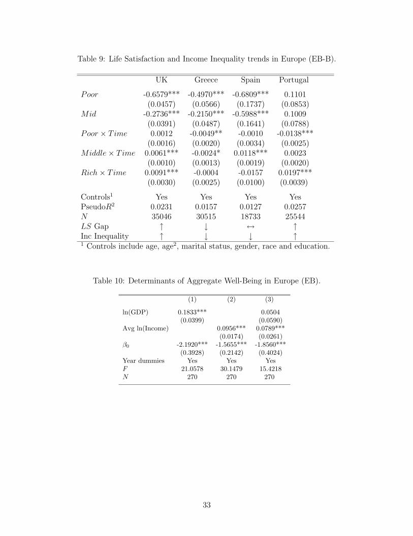
Table 9: Life Satisfaction and Income Inequality trends in Europe (EB-B).

UK Greece Spain Portugal

Poor -0.6579*** -0.4970*** -0.6809*** 0.1101(0.0457) (0.0566) (0.1737) (0.0853)

Mid -0.2736*** -0.2150*** -0.5988*** 0.1009(0.0391) (0.0487) (0.1641) (0.0788)

Poor × Time 0.0012 -0.0049** -0.0010 -0.0138***(0.0016) (0.0020) (0.0034) (0.0025)

Middle× Time 0.0061*** -0.0024* 0.0118*** 0.0023(0.0010) (0.0013) (0.0019) (0.0020)

Rich× Time 0.0091*** -0.0004 -0.0157 0.0197***(0.0030) (0.0025) (0.0100) (0.0039)

Controls1 Yes Yes Yes YesPseudoR2 0.0231 0.0157 0.0127 0.0257N 35046 30515 18733 25544LS Gap ↑ ↓ ↔ ↑Inc Inequality ↑ ↓ ↓ ↑1 Controls include age, age2, marital status, gender, race and education.

Table 10: Determinants of Aggregate Well-Being in Europe (EB).

(1) (2) (3)

ln(GDP) 0.1833*** 0.0504(0.0399) (0.0590)

Avg ln(Income) 0.0956*** 0.0789***(0.0174) (0.0261)

β0 -2.1920*** -1.5655*** -1.8560***(0.3928) (0.2142) (0.4024)

Year dummies Yes Yes YesF 21.0578 30.1479 15.4218N 270 270 270

33

References

[Andrew E. Clark and Shields(2008)] P. F. Andrew E. Clark and M. A. Shields. Relativeincome, happiness, and utility: An explanation for the easterlin paradox and otherpuzzles. Journal of Economic Literature, 46(1):95144, June 2008.

[Barrington-Leigh and Helliwell(2008)] C. P. Barrington-Leigh and J. Helliwell. Empathyand emulation: life satisfaction and the urban geography of veblen effects. Universityof British Columbia, mimeo, 2008.

[Begley()] S. Begley. Why money doesnt buy happiness. Newsweek.

[Easterlin(1974)] R. A. Easterlin. pages 235–247, July 1974.

[Frey and Stutzer(2002)] B. S. Frey and A. Stutzer. What can economists learn from hap-piness research? Journal of Economic Literature, XL:402–435, June 2002.

[Kimball and Silverman(2008)] M. Kimball and D. Silverman. Subjective well-being andbereavement. University of Michigan, mimeo, 2008.

[Layard(2005)] R. Layard. Rethinking Public Economics: The Implications of Rivalry andHabit. 2005.

[Luttmer(2004)] E. F. Luttmer. Neighbors as negatives: Relative earnings and well-being.Quarterly Journal of Economics, 120(3):9631002, 2004.

[Miles Kimball and Tsutsui(2006)] F. O. Miles Kimball, Helen Levy and Y. Tsutsui. Un-happiness after katrina. University of Michigan, mimeo, January 2006.

[OECD(2007)] OECD. Organization for economic cooperation and development, 2007.

[of Pennsilvanya(2007)] U. of Pennsilvanya. World penn tables, 2007.

[Rafeal Di Tella and MacCulloch(2004)] J. H.-D. N. Rafeal Di Tella and R. MacCulloch.Happiness adaptation to income and to status in an individual panel. Harvard BusinessSchool and Imperial College London, mimeo, 2004.

[Stevenson and Wolfers(2008a)] B. Stevenson and J. Wolfers. Economic growth and subjec-tive well-being: Reassessing the easterline paradox. Wharton University of Pennsylva-nia, mimeo, April 2008a.

[Stevenson and Wolfers(2008b)] B. Stevenson and J. Wolfers. The paradox of declining femalhappiness. Wharton University of Pennsylvania, mimeo, April 2008b.

34