Inequality and happiness: When perceived social mobility and

MPRAMunich Personal RePEc Archive

Inequality and happiness: Whenperceived social mobility and economicreality do not match.

Christian Bjornskov and Axel Dreher and Justina A.V.

Fischer and Jan Schnellenbach and Kai Gehring

University of Aarhus, University of Freiburg, Heidelberg University,University of Mannheim, University of Oradea

7. March 2013

Online at http://mpra.ub.uni-muenchen.de/44827/MPRA Paper No. 44827, posted 7. March 2013 16:02 UTC

http://mpra.ub.uni-muenchen.de/

http://mpra.ub.uni-muenchen.de/44827/

Inequality and happiness:

When perceived social mobility and economic reality do not match

Christian Bjørnskov a, Axel Dreher b, Justina A.V. Fischer c,

Jan Schnellenbach d, Kai Gehring e

March 06, 2013 Abstract We argue that perceived fairness of the income generation process affects the association between income inequality and subjective well-being, and that there are systematic differences in this regard between countries that are characterized by a high or, respectively, low level of actual fairness. Using a simple model of individual labor market participation under uncertainty, we predict that high levels of perceived fairness cause higher levels of individual welfare, and lower support for income redistribution. Income inequality is predicted to have a more favorable impact on subjective well-being for individuals with high fairness perceptions. This relationship is predicted to be stronger in societies that are characterized by low actual fairness. Using data on subjective well-being and a broad set of fairness measures from a pseudo micro-panel from the WVS over the 1990-2008 period, we find strong support for the negative (positive) association between fairness perceptions and the demand for more equal incomes (subjective well-being). We also find strong empirical support for the predicted differences in individual tolerance for income inequality, and the predicted influence of actual fairness.

Keywords: Happiness, life satisfaction, subjective well-being, inequality, income distribution, redistribution, political ideology, justice, fairness, World Values Survey JEL codes: I31, H40, D31, J62, Z13 Acknowledgements: An earlier version was circulated under the title “On the relation between income inequality and happiness: do fairness perceptions matter?”. We thank Manfred Holler, Ekaterina Uglanova, participants at the 2007 IAREP conference (Ljubljana), and the 2008 CESifo workshop on Ethics and Economics (Munich), and an anonymous referee for comments on the earlier draft and Jamie Parsons for proofreading. Justina Fischer thanks the Marie Curie fellowship schemes (ENABLE, TOM) for financing this research and the Stockholm School of Economics, the Thurgau Institute for Economics and the University of Hamburg for their hospitality. a Department of Economics and Business, Aarhus University, Fuglesangs Allé 4, DK-8210 Aarhus V, Denmark; phone: +45 87 16 48 19; e-mail: [email protected]. b Heidelberg University, Alfred Weber Institute for Economics, Bergheimer Strasse 58, 69115 Heidelberg, Germany, CESifo, Germany, IZA, Germany, University of Goettingen, Germany, and KOF Swiss Economic Institute, Switzerland; e-mail: [email protected]. c University of Mannheim, Department of Economics, L7, 3-5, 68131 Mannheim; University of Oradea, Department of International Relations, Oradea, Romania; e-mail: [email protected]. d Walter Eucken Institut, Goethestrasse 10, 79100 Freiburg, Germany; Heidelberg University, Alfred Weber Institute for Economics, Bergheimer Strasse 58, 69115 Heidelberg, Germany; e-mail: [email protected]. e University of Goettingen, Platz der Goettinger Sieben 3, 37073 Goettingen, Germany, Heidelberg University, Germany; e-mail: [email protected]

2

Inequality is undoubtedly more readily borne, and

affects the dignity of the person much less, if it is

determined by impersonal forces than when it is

due to design.

Friedrich Hayek

(1944: 117)

1. Introduction

Since Abba Lerner’s classic contributions from the 1930s, welfare economics has argued that

income redistribution can increase overall welfare in a society with an unequal distribution of

incomes, due to the decreasing returns to income caused by an assumed strict concavity of

individual utility functions (Lerner, 1944). This view implies that most people in societies

characterized by a highly skewed income distribution should, all other things being equal, be

observed to experience lower levels of utility than those living in more equal societies. With

the advent of the economics of happiness, it has become possible – and fashionable – to test

this implication on individuals’ self-reported life satisfaction, which arguably proxies for the

economic concept of ‘utility’.1 If Lerner’s implication – and indeed standard economic theory

– holds, we would expect to see a clear negative association between income inequality and

life satisfaction of the average person. Such empirical results would also be in line with the

more recent theoretical model by Fehr and Schmidt (1999), taking account of social (other-

regarding) preferences in individuals’ utility functions, equally predicting a negative

relationship between inequality and happiness.

Even though this straightforward microeconomic approach predicts that overall and

average welfare in an economy decrease with income inequality, the empirical literature on

the association between income inequality and happiness2 has yielded ambiguous findings.3

1 For an overview of the economic, sociological and psychological concepts of subjective well-being and validity studies on its alternative measures, see Diener et al. (2008), Fischer (2009a), and Veenhoven (2000). 2 In this paper, we use the terms ‘happiness’, ‘subjective well-being’, and ‘well-being’ interchangeably. 3 In a related field of research Clark, Frijters and Shields (2008), Layard, Mayraz and Nickell (2009), and Fischer and Torgler (2013) among others, use micro data to analyze income inequality effects through social

3

One of the first empirical contributions, Alesina et al. (2004), identify a negative association

between income inequality and happiness for 12 European countries that remains statistically

insignificant for most U.S. states. Explaining their results, the authors hypothesize that

differences in perceived and actual social mobility exist between these two subsamples.

Extending the sample to 30 OECD countries, Fischer (2009b) reports a negative association

between individual life satisfaction and inequality in final income, but not for market-

generated income inequality – potentially indicating that it is actual consumption on which

social comparisons are based. 4 In a world sample, however, the large-scale robustness

analysis in Bjørnskov, Dreher and Fischer (2008) suggests that the skewedness of the income

distribution does not, in general, directly affect individual happiness.

In this paper, we investigate the relationship between inequality and happiness,

extending previous research in two dimensions: First, we allow individuals’ subjective

perceptions of ‘fairness’ attributed to the income-generating process to affect the association

between life satisfaction and income inequality. Second, we allow for differences in the actual

fairness of the income generation process across countries, expecting that these affect how

fairness perceptions influence the inequality-happiness-relation. Indeed, Grosfeld and Senik

(2009) show that in the transition country Poland, income inequality at first contributed

positively to people’s happiness from 1992 to 1996, possibly because it was associated with

given and perceived good economic opportunities (see also Hirschman and Rothschild, 1973).

In contrast, in the later period from 1997 onwards, it affected people’s happiness negatively,

possibly because lower actual social mobility mismatched with the high perceptions people

still had. Alesina et al. (2004) already conjectured that inequality might affect people's

happiness with specific values and specific views on social mobility within the same societies

differently, even if inequality in general is not associated with happiness.

We present a stylized theoretical model, which serves to illustrate our main arguments

and allows us to derive some testable hypotheses. This model analyzes individual labor-

comparisons where persons compare their income with a reference level. In our study, inequality rather refers to differences in absolute income across persons and the presence of redistributive government activities. 4 This is in line with Hopkins’ (2008) ‘rivalry model in conspicuous consumption’ according to which income inequality increases individual utility under certain conditions (high income and consumption levels, and a dense income distribution), as greater incentives to compete in consumption are generated.

4

market participation on the extensive and the intensive margin, depending on expected (i.e.,

perceived) fairness of the income-generating process. In the model, a society is considered

fairer the closer the relationship between individual effort and market outcome is. Actual

fairness can therefore also be interpreted as a measure of social mobility, because with

increasing objective fairness, inherited social status loses relevance. Our model allows

systematic and persisting incongruences between actual and perceived fairness. The model

predicts that persons with higher perceived fairness will, on average, experience higher levels

of utility and be less in favor of income redistribution.

We argue that in a society where the distribution of individual inherited starting

positions is sufficiently skewed to the right (i.e., where relatively few individuals “are born

with a silver spoon”), subjective fairness perceptions are the main driver of investments into

effort on the labor market. Using a standard notion of status utility, we then show that

individuals with high subjective fairness perceptions react more favorably to income

inequality than those with low fairness perceptions. Finally, we demonstrate that the

composition of the pool of individuals with high subjective fairness perceptions

systematically differs between countries with high and low actual social mobility. In countries

with high actual mobility, more individuals with low ex ante fairness perceptions who invest

little into effort are surprised by higher than expected incomes, and thus correct their ex post

fairness perceptions upward. In countries with low actual mobility, these positive surprises are

fewer, and thus the pool of high fairness individuals is composed of individuals with, on

average, higher incomes and higher subjective well-being. Somewhat paradoxically, via this

mechanism high actual social mobility thus reduces the positive mediating effect that high

subjective fairness perceptions have on the impact of inequality on life satisfaction.

To explore the link between perceptions of fairness, social mobility, inequality, and

happiness empirically we use data from the World Values Survey over the 1990-2008 period

and estimate a happiness function. We employ standardized Gini coefficients to measure

income inequality, different proxies for individuals’ perceived fairness of the income

generating process, and the interactions of inequality with these proxies. The empirical

analysis aims to explore whether and to what extent perceived fairness mediates the potential

5

effects of inequality, differentiating between countries with low and high actual social

mobility. We also investigate the relation between fairness perceptions and the demand for

redistribution, mediating the impact of fairness on life satisfaction.

We find that persons who believe the income generating process in their society to be

fair appear to be happier and demand less income equalization by (and redistribution from)

the government. As predicted by the model, we also find strong empirical support for the

more positive effect of inequality for individuals with high fairness perceptions in countries

with unfavorable institutions hampering social mobility. Consistent with our model, for

countries with high levels of actual intergenerational social mobility in terms of earnings –

thus triggering a close relationship between individual effort and market outcomes – the

effects of income inequality and fairness perceptions appear rather weak or disentangled in

their interactions. The interaction results are corroborated in samples based on measures of

actual mobility through the education system.

Section 2 presents a literature review, and our stylized theoretical model motivating

the empirical analysis. From the model we then derive testable hypotheses. We describe our

data and methods in Section 3, while Section 4 presents the results. The final section

concludes and discusses the implications of our findings.

2. Happiness, inequality and fairness: Theory

2.1. Preliminary considerations

In 1944, Austrian economist and social philosopher Friedrich Hayek (1944: 88) argued “To

produce the same results for different people, it is necessary to treat them differently. To give

different people the same objective opportunities is not to give them the same subjective

chances.” From this follows, as Hayek suggested, that forcing individuals’ outcomes to be

identical and ‘fair’ implies treating people unequally, and, thus, ‘unfairly’. The relation

between what could be termed ‘fairness’ or other moral judgments of processes and outcomes

and social inequality is therefore far from simple and straightforward.

6

The treatment of ‘utility’ in economics literature, both by the empirical research on

happiness as well as standard economic theory, has usually focused on pure outcomes and

neglected social comparisons. Yet, individuals do not only derive satisfaction from outcomes,

but probably compare themselves to others, and also enjoy ‘procedural utility’ (Veblen 1899,

Fehr and Schmidt, 1999; Frey and Stutzer, 2005). If people gain the impression that processes

affecting their own situation are ‘fair’, they are not only likely to directly derive procedural

utility from that fact, but also tend to evaluate the outcomes of these processes differently than

if their subjective perception of the process is that it is ‘unfair’. For example, most people

strongly dislike losing games or sports matches, but the impact of a loss is much stronger if

they have the – reasonable or unreasonable – impression that their opponent has not played by

the rules. Similarly, Stutzer and Frey (2003) show that two-thirds of the beneficial effects of

people’s influence in the political decision-making process is not through their impact on

resulting policy outcomes, but through the procedural utility gained from participation and

civic engagement. Experimental evidence tends to support Hayek’s broad argument: Recent

economic experiments reveal that inequality in profits is the more tolerated (by otherwise

generally inequity-averse individuals) the more the process leading to its generation was

perceived as ‘fair’. Experimental research has even identified the corresponding neurological

process in the reward center of the human brain (see Hopkins, 2008, for a summary).

To sum up, economic experiments show that if the process of reaching an outcome has

been fair, then subjects in general bear an adverse outcome more easily. In contrast to our

study, the set-up of these experiments is fairly simple, allowing actual fairness of the process

and perceived fairness of the distribution process to coincide. However, one decisive

contribution of our paper is to draw conclusions differentiating between actual and perceived

fairness, which may or may not overlap, reflecting more complex real-world characteristics,

which do not allow individuals to objectively observe actual social mobility in their societies.5

These theoretical and experimental arguments can be applied to individuals’

evaluations of the distribution of income in society. Their subjective evaluation of the

outcome – the inequality of incomes – is likely to depend on their perceptions of the processes 5 Indeed, our model suggests that if perceived fairness is high and actual fairness has a corresponding level, the positive effect of inequality on subjective well-being rises with perceived fairness.

7

creating the distribution and their evaluations of the fairness of those processes. Such

conjecture has already been made by Alesina et al. (2004) to explain the differential effect of

income inequality on happiness of survey respondents in the United States compared to those

in Western Europe. For a sample of 30 OECD countries in the WVS, Fischer (2009b) finds

that in a socially mobile society (from the interviewees’ points of view) the negative effect of

income inequality on well-being is mitigated, if not overcompensated for. Likewise, in

economic laboratory experiments, Mitchell et al. (1993: 636) find that “inequality becomes

more acceptable as people are better rewarded for their efforts,” which can be interpreted as

an indication for a mediating effect of the fairness of the distribution process of ‘rewards’, i.e.,

wage incomes, on the relationship between inequality and happiness.

In this paper, we define an income generating process as ‘fair’ if there is a direct link

between own investment in human capital, on-the-job effort and individual economic

outcome. The weaker this link becomes, i.e., the more the individual outcome depends on

chance and at the same time is related to inherited starting positions, the less fair the income

generating process is. This would also be the case if income differences were caused mainly

by individual differences in innate talent or ability that cannot be compensated for by effort.

Such initial endowments could also include inherited wealth. On the other hand, if

individuals’ perceptions of society indicate that ‘someone’ – either individually or collectively

(e.g., through political decision-making) – is responsible for the shape of the income

distribution, moral judgments on fairness will arguably come to rest on a different foundation.

The difference between actual (objective) and perceived (subjective) fairness in the

income generation process is often not clearly recognized by the early theoretical and

empirical literature on happiness or preferences for redistribution. Most studies implicitly –

and in the case of Alesina et al. (2004) explicitly – assume that subjectively perceived and

objectively existing fairness in society correspond perfectly. However, the empirical

happiness analysis for 30 OECD countries by Fischer (2009b) suggests that perceived and

actual social mobility in society are not necessarily strongly correlated. For this reason, we

explicitly differentiate between actual and perceived fairness and put them in a systematic

relation. In particular, we hypothesize that whether the happiness effects of income inequality

8

are aggravated or reduced by fairness perceptions for most of the population hinges on

whether perceived and actual fairness coincide or diverge.

Fairness perceptions can also be argued to diverge according to political convictions.

Typically, left-wing parties place more weight on equity of outcomes (so-called ‘social

justice’), while right-wing governments place more weight on efficiency and equality in

opportunities. This is observed as voters’ definitions of fairness differ systematically between

parties (Scott et al. 2001). Fundamental differences in fairness perceptions would thus suggest

that left-wing voters are sensitive mainly to income inequality, but less to procedural fairness

as a determinant of market income (see also the empirical test in Fischer 2009b). In contrast,

right-wing voters have offsetting efficiency concerns, which lead them to focus more on

equality of opportunities, and to accept the resulting income inequality more easily. From a

conservative perspective, relatively large income differences might be seen as an indication

that individuals who work hard receive their just desserts. Indeed, Alesina et al. (2004) find

that left-wing voters are more concerned about income inequality than right-wing or centrist

voters, both in Europe and the United States. We therefore employ the respondent’s political

ideology as one proxy of her fairness perception.

In the course of this analysis, we predict a negative relationship between fairness

perceptions and the demand for income redistribution, which we also test against our data.

The relation between social mobility (perceptions) and the preference for equal incomes has

been analyzed in a few previous studies. Ravallion and Lokshin (2000), using Russian micro

data, were the first to show that self-assessed expected own social mobility, or the belief of

being on a rising income trajectory, leads to lower demand for redistribution. Corneo and

Gruener (2002) present a ‘public values effect’ model concluding that “an individual who

believes in the importance of personal hard work [for income] is expected to oppose

redistribution” (ibidem: 86), preceding the similar arguments in Alesina et al. (2004). In

Corneo and Gruener’s (2002) logit regressions, run with about 30 countries in various

International Social Survey Programme (ISSP) waves on the question ‘Government should

reduce inequality’, both generalized fairness perceptions and perceived past social mobility

9

reduce the demand for equalizing incomes.6 In contrast, persons reporting that ‘they would

gain [from redistribution]’ are in favor of such government policy. Population preferences for

and against redistribution are captured by country-fixed effects, an approach that we will

follow below.

A negative relationship between personal income and preferences for redistribution is

not only shown in Corneo and Gruener (2002), but also by Alesina and La Ferrara (2005).

Using U.S. General Social Survey (GSS) data, the latter corroborate the negative relation

between perceived equal opportunities, subjective income prospects, income, and a history of

past social mobility, with a preference for income redistribution.7 Exploiting the longitudinal

nature of their panel data, Alesina and La Ferrara (2005) construct two objective measures of

actual income prospects, at the individual and state level. They find both to be strongly

negatively related to individual demand for more equal incomes. Contrasting results are

reported in Clark and D’Angelo (2008) for the British Household Panel Survey (BHPS) who

identify a positive association between own experienced social mobility (‘having higher

socio-economic status than parents’) and being in favor of having capped incomes, or state-

ownership, and being left-wing.8

In the following, we develop a simple workhorse model, illustrating the potential

impact of income inequality and fairness perceptions on individual well-being.

2.2. The basic set-up of the model

Following, among others, Blanchflower and Oswald (2004), we assume that reported

subjective well-being or ‘happiness’ of an individual i is an increasing function of her

instantaneous, directly unobservable utility where i is an error-term:

6 Fairness perceptions are measured by the question ‘hard work is the key [to success]’, while social mobility experience is captured by the variable ‘better off than father’. 7 Preference for redistribution is measured by the question ‘Should government reduce income difference between rich and poor?’. Past history of social mobility is measured by ‘having a job prestige higher than father’s’, and subjective income prospects are proxied by ‘expect a better life’. Equal opportunities as source of economic success are approximated by the question ‘Get ahead: hard work’, while unequal opportunities are approximated with the statement ‘Get ahead: luck/help’. 8 This study employs the measure ‘The government should place an upper limit on the amount of money that any one person can make’, which is not fully comparable to that used in previous empirical analyses.

10

(1)

The error term reflects unobservable differences across individuals, such as different

subjective interpretations of the ordinal scale on which individual well-being is reported. This

assumption allows us to focus on standard economic utility considerations in the theoretical

analysis, i.e., on the underlying economic forces that influence individual welfare.

We assume that utility is concave in income and that effort invested to earn income

has a negative and quadratic direct effect on utility.

(2)

where

(3)

and is a status and identity utility which is explained in detail below.

Income increases with effort according to the strictly concave function g. The

parameter is a society-wide fairness parameter. The closer its value is to one, the

more reliable is the impact of individual effort on individual income. The value of this

parameter is identical for all individuals. On the other hand, is an idiosyncratic

parameter reflecting, for example, the family background, or the place of birth of an

individual, or access to personal networks that may be instrumental in generating incomes. In

general, captures anything in the personal background of an individual that may make it

more difficult for her to earn an income based upon her own effort.

We assume that the true value of is unknown to the individual decision-makers.

They can certainly observe the institutional framework of their society, but the web of formal

and informal institutions that characterizes any modern society is generally complex enough

to make any exact ex ante knowledge of the true value of extremely unlikely. Every

individual therefore bases her decisions on her own estimate , which denotes her perceived

Wi w(ui ) i

yi

ui v(yi )1

2ei

2

yi g(ei ) 1 1 1 i

[0,1]

i [0,1]

i

˜ i

11

fairness. 9 The idiosyncratic parameter is assumed to be drawn randomly from an

individual-specific distribution characterized by the continuous and unimodal pdf with

support . Let denote the expected value of the idiosyncratic parameter for individual i.

We assume that the distribution of over the population is skewed to the right, and also

unimodal. We further assume that all individuals know their own . They do, however, not

observe the value of that is eventually drawn. They only observe income and effort, but

have no definitive knowledge about how much of the result is due to bad (good) institutions,

or an (un-)lucky draw of the idiosyncratic parameter. Furthermore, we assume that is

inherited: Individuals from poorer families or worse neighborhoods are characterized by

lower values of .10 However, even individuals from unfavorable backgrounds have a chance

to draw a favorably high from the distribution.

The status and identity utility consists of two components

(4) yi y* i, i 2

(yi y)

where straightforwardly signifies a status utility, as a concave and strictly increasing

function of the difference between individually realized and average income. We assume that

(0) 0 . This follows a standard approach of assuming that individuals use some reference

income to evaluate their own status (e.g., Ederer and Pattaconi 2010, Luttmer 2005). The first

term is the highest identity utility attainable by the individual. It is reduced according to a

quadratic loss function, which has a simple economic interpretation. Benchmark income y* is

the income that the individual would expect to be earned by an individual of her type and

given her fairness estimate i , if she invests the optimal level of effort e*. In other words, it

is the income expected from an individual of her type, given the perceived circumstances. If

9 Piketty (1995) has shown in a model where individual income is also determined by societal fairness and individual influences that differences in fairness estimations may prevail in an equilibrium with full Bayesian rationality. 10 Note that there is emphatically no genetic inheritance assumed to be at work here. This approach simply captures the empirical regularity that individuals from low-income families often find it more difficult to rise into high-paying positions than those who already have a high-income background. In a utopian situation with

completely fair institutions ( ), the impact of the idiosyncratic parameter would be cancelled out completely.

i

f i ( i )

0,1 ˆ iˆ i

ˆ ii

ˆ i

ˆ ii

1 ˆ i

12

her realized income yi is less than this expectation, a disutility arises from the feeling of

being an underachiever. If, on the other hand, it is higher, then a disutility arises out of the

feeling of having an unfair advantage from having drawn a favorable value of i . Thus, the

quadratic loss function measures if and how far the individual deviates from her peer group,

given the perceived circumstances. In this respect, we follow a standard approach of

integrating identity utility (e.g., Akerlof and Kranton 2000; Georgiadis and Manning 2012,

Casey and Dustmann 2010).

We assume the following sequence of events: 1. Individuals decide on their level of

effort by maximizing (2); 2. Their own income levels and the average income level of the

population are revealed to the individuals; 3. Individuals may revise their ex ante fairness

perceptions.

Individuals choose effort in order to maximize their expected utility. We assume Nash

behavior, i.e., individuals neglect the impact of their own choices on y* and y .

(5) iiiiiiiiiie

deeevf

1

0

2

0)~,ˆ,(

2

1)~,ˆ,()(max

This directly leads to the first order condition

(6) E v'(ei,i , i ) '(ei ,i, i )

ei .

2.3. Expected and actual utility, effort and reported happiness

From (6), we can infer individually optimal effort levels as functions of the other model

parameters:

(7) with and .

Status utility leads individuals to increase their effort over the level they would choose

without status competition, but this effect is tempered by the prospect to enjoy identity utility

by conforming to one’s peer group. Since both the individual expected marginal productivity

of effort and the expected peer group income strictly increase with i , optimal individual

effort is strictly increasing in this parameter.

ei* ei

* ˜ i, ˆ i ei ˜ * 0 e

i ˆ * 0

13

Deriving an indirect utility function V from (2) and using the envelope theorem reveals

that V i 0 , i.e., expected utility is increasing in . However, a range of actually realized

individual utility levels in the population corresponds to any value of , each depending on

the individually drawn value . How will i respond if ? The key

to the answer is the identity utility term. At this point in time incomes are revealed and effort

cannot be changed. But in order to reduce the value of the loss function in (4), the individual

has a strong incentive to adjust her fairness perception. If , the individual will want to

avoid the explanation of a lucky draw of i , which would imply free-riding to a higher than

expected income, using, for example, good looks and personal networks. This unfavorable

explanation can be avoided by increasing the assumed value of . Note that given (3), any

higher than expected income can be individually explained by claiming i i and adjusting

the fairness perception upwards. This can even be rationalized by the individual, since she

will be able to find individuals from her peer group who had a higher ex ante fairness

perception, thus invested more effort, and realized a similar income without being surprised.

As long as incomes are observable, but effort is not, the update of the fairness perception is

not only a matter of self-justification, but also plausible.

If , the opposite reaction is likely: will be revised downward in an attempt to

explain lower than expected individual incomes with unfavorable institutional circumstances.

Note, however, that given (3), this may not in every case be entirely possible. The reason is an

asymmetry: Completely fair institutions cancel out the impact of the idiosyncratic parameter.

Thus, it is possible to explain any positive surprise with a sufficiently high fairness parameter.

A value close to zero of the fairness parameter, on the other hand, implies that the

idiosyncratic parameter has full impact. Thus, an individual with a realized value of i very

much below its expected value may not be able to completely cancel out the term of the loss

function by assuming a low fairness parameter. Put differently, individuals who experience

negative income surprises reduce the impact of the loss function to some extent by assuming

an unfair institutional framework, but they may even then be left with a residual loss of

identity utility.

˜ i˜ i

i

˜ i

˜ i

14

In any event, the tendency to reduce a loss of identity utility by suitably adjusting

one’s fairness perception implies an unambiguous relationship between fairness perception

and individual welfare. This leads us to our first proposition:

Proposition 1. We expect the relationship between subjective individual perceptions about

the fairness of the market income generation process and individual welfare to be positive.

2.4. Preferences for income redistribution and individual welfare

Let there be a simple, redistributive tax and transfer system, which consists of a proportional

income tax with rate t levied on labor income, and of a guaranteed transfer income paid

to those individuals who do not earn a market income.11 To keep matters simple, we assume

that the government commands no screening technology that would allow it to distinguish

between voluntary and involuntary unemployment. Individuals therefore compare expected

utilities inside and outside the labor market, and participate only if the former exceeds the

latter. Thus, for any given tax and transfer system there exists a combination of low

levels of and where the individually expected marginal productivity of effort is so small

that the individual decides against labor market participation. In general, higher perceived

fairness yields higher labor market participation rates even in groups who expect relatively

lower values of . Redistribution is ex ante only in the interest of individuals who plan not to

participate in the labor market.

The relationship between fairness perceptions and preferences for redistribution is

reinforced if we also allow for ex post adjustments of fairness perceptions as discussed above.

Suppose the redistribution scheme is extended such that individuals who participate, but earn

a surprisingly low income, are paid a transfer until they reach a net income of . Those

benefiting from such a scheme would all be individuals with , who revise their fairness

perceptions downward ex post. In other words, all transfer-recipients are characterized by low

fairness perceptions: either because they already had them ex ante, and decided not to

11 See, e.g., Harms and Zink (2003) for a survey of the political economy of income redistribution.

yT (t)

t,yT (t) ˜ i

i

yT

15

participate in the labor market, or because they were disappointed by their individual market

outcome and accordingly revised their fairness perception downwards ex post. This revision

leads to an ex post fairness perception which lies below the ex ante threshold for labor market

participation. However, any investments into effort are obviously sunk and cannot be

retrieved. This leads us to introduce our second proposition:

Proposition 2. The likelihood that a randomly drawn individual will have a preference for

increased redistribution increases with a decreasing individual fairness perception.

Therefore, a stronger preference for redistribution is also expected to be negatively

correlated with individual welfare.

2.5. Fairness, inequality and self-reported happiness

Our model contains different mechanisms that yield income inequality. The ex post market

income of individual i is

(8) .

First of all, income inequality generally stems from the idiosyncratic parameter. The

larger the variance of in the population, the larger the inequality of incomes ceteris paribus

will be. This will normally also imply a large variance of , and thus of individually chosen

effort levels. Similarly, a larger variance of individual beliefs also eventually results in

larger income inequality, through the establishment of a larger variety in the individual

choices of effort levels, with any given distribution of idiosyncratic parameters.

We have seen in the discussion leading to Proposition 1 that higher income levels are

associated with higher fairness perceptions, both ex ante due to increased effort, and ex post

due to revised fairness perceptions. In combination with the status utility term in (4), we

immediately observe that individuals that benefit from increasing income inequality via a

positive status utility are characterized by above-average incomes and thus relatively high

yi* g ei

*( ˜ i, ˆ i ) 1 1 1i

i

ˆ i˜ i

16

fairness perceptions. There may be individuals with a high value of i and a low fairness

perception, whose high expected idiosyncratic parameter leads to a high effort and income

level. However, if the distribution of i in the population is sufficiently skewed to the right,

the number of these types of individuals will be small and dominated by those who are

characterized by high incomes and high fairness perceptions.

Proposition 3. If the fraction of individuals who are characterized by high expected values of

the idiosyncratic parameter is sufficiently small, then those individuals who have high

fairness perceptions will, on average, react more favorably to income inequality than

individuals with low fairness perceptions.

Finally, we look beyond fairness perceptions and consider the impact of actual fairness and

income inequality on subjective well-being in different groups of the population. A higher

value of the actual fairness parameter π reduces the impact of the idiosyncratic parameter on

individual incomes. In the limiting case of perfect fairness, the impact of the latter parameter

disappears completely, and there is a deterministic link between (differences in) individual

effort and income (inequality). According to (3), this implies that all individuals with i 1

and a i 1 will earn a higher than expected income, and accordingly increase their fairness

perception ex post. This implies that all individuals who invest relatively little effort due to

unfavorable ex ante expectations revise their fairness perceptions upward. These, however,

are individuals who earn higher than expected but still relatively low absolute incomes, due to

their low effort levels.

Suppose, on the other hand, that actual fairness is very low. Then the only individuals

who benefit from higher than expected incomes, and who update their fairness perception

accordingly (and mistakenly), are those who draw a higher than expected value i i . This

implies that fewer individuals with low effort levels, and thus low absolute incomes, will

increase their fairness perceptions than in the case of high actual fairness.

17

At the other end of the effort scale, we know that individuals who decide to invest high

levels of effort must from the outset be characterized by a high value of i and/or i . Given

our assumption that the distribution of i is skewed to the right, most individuals who decide

to invest high effort are characterized by high initial fairness perceptions. Hence, if we

compare the pool of individuals with high fairness perceptions under high and low actual

fairness, we expect its composition to differ under both regimes. With low actual fairness,

relatively few positively surprised low-effort (and thus low-income) individuals enter the pool

of high-fairness perception individuals. Thus, the average high-fairness individual benefits to

a large extent from status utility and income inequality. With high actual fairness, more low-

effort and low-income individuals ex post enter the group of high-fairness individuals. With

on average more low-income individuals in this group, the average positive effect of status

utility (and income inequality) must decline. This leads us to

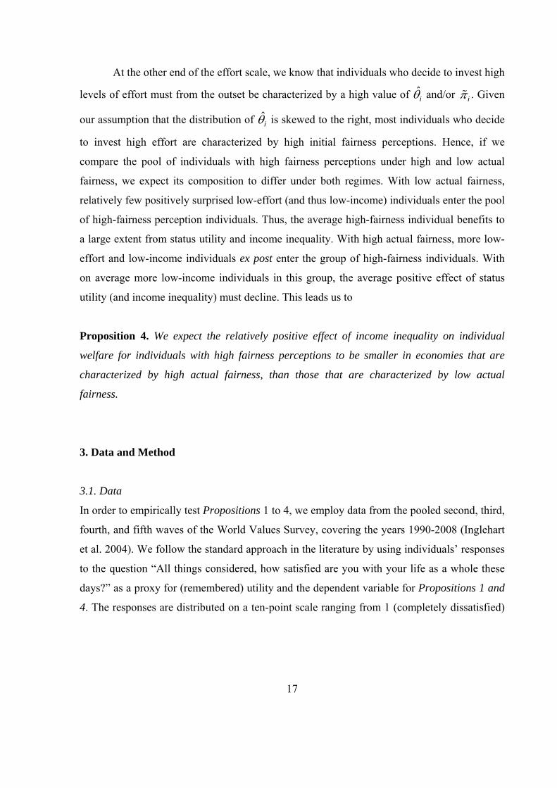
Proposition 4. We expect the relatively positive effect of income inequality on individual

welfare for individuals with high fairness perceptions to be smaller in economies that are

characterized by high actual fairness, than those that are characterized by low actual

fairness.

3. Data and Method

3.1. Data

In order to empirically test Propositions 1 to 4, we employ data from the pooled second, third,

fourth, and fifth waves of the World Values Survey, covering the years 1990-2008 (Inglehart

et al. 2004). We follow the standard approach in the literature by using individuals’ responses

to the question “All things considered, how satisfied are you with your life as a whole these

days?” as a proxy for (remembered) utility and the dependent variable for Propositions 1 and

4. The responses are distributed on a ten-point scale ranging from 1 (completely dissatisfied)

18

to 10 (completely satisfied), with a sample mean of about 6.3.12 In order to estimate a set of

relevant personal characteristics forming the core of individuals’ happiness functions, we rely

on the robust baseline model in Bjørnskov, Dreher and Fischer (2008) and Fischer (2009c).

We include country-fixed effects, wave-fixed effects, and their interactions, to control for any

variables that do not vary within a country, over time, or are constant within a certain country

and wave, and that might be correlated with our variables of interest. This extensive set of

fixed effects minimizes the possible influences of omitted variables bias, given that we

identify the effects of our variables of interest using variation at the individual level holding

country-, period-, and country-period fixed effects constant. At the individual level, we

include measures of age, gender, family type, religion, religiosity and spirituality, and age

cohort effects.13 We also include measures of education, income and occupational status that,

according to the theoretical model, mediate an individual’s subjective success probability

(fairness perception). Table 2 excludes these variables so that we can assess the importance of

this transmission channel.

Measures of vertical and horizontal trust (such as confidence in political institutions

and trust in other people) are not part of the baseline model as they may be strongly correlated

with perceived fairness and could thus be transmission channels for our variable of main

interest.14 The baseline sample includes about 300’000 persons in more than 80 countries but,

due to data availability, it is much smaller in most regressions, depending on the employed

12 The WVS includes questions on both life satisfaction and happiness, but the correlation between happiness and satisfaction is surprisingly low (rho = 0.44). We opt for using the life satisfaction question since: 1) translation problems seem to yield cross-country comparisons of answers to the other question less comparable and; 2) the happiness question is more likely to capture the affective component of subjective well-being rather than its cognitive component (for a discussion, see Fischer 2009a). 13 Arguably, more optimistic people could be more likely to be happier and at the same time perceive fairness to be more prevalent. The 1990-wave of the World Value Survey contains two questions that relate to optimism, which we use to test for this possibility: (1) "I am good at getting what I want" and (2) "I usually count on being successful in everything I do." When we re-estimate all regressions using one of these two variables, respectively, our main results are not affected. We report these results in the Appendix Tables B.2. and B.3.While we are thus confident that our results are not due to the omission of optimism, other omitted individual-specific variables could bias our results, as in any comparable study. While we control for many individual-specific variables and address omitted variable bias at the country-level by our extensive set of fixed effects, a bullet-proof test of our theory would require an exogenous instrumental variable or "true" panel data. We unfortunately have neither of those. 14 Note that the inclusion of a measure of horizontal trust does not alter the main results of our analysis however (e.g., in Tables 6 and 7), but does reduce the size of the regression samples.

19

fairness measure. The baseline results for the micro-level determinants of subjective well-

being (SWB) in the present sample are similar to those in Bjørnskov, Dreher and Fischer

(2008) – they are reported in Column 1 of Table A1 in Appendix A, while Appendix B

presents descriptive statistics.15

Measures of self-report procedural fairness and demand for income redistribution

Individuals’ fairness evaluations of income inequality are approximated using definitions of

fairness in the income generation process in the labor market. They include measures of social

mobility in the labor market such as whether hard work determines economic success. All

fairness perception proxies are constructed as dichotomous variables, taking on the value ‘1’

if the respondent believes that procedural fairness is present in society, and ‘0’ if otherwise.

These definitions of fairness perceptions have also been employed in previous studies such as

Corneo and Gruener (2002) and Alesina and La Ferrara (2005). In addition, we approximate

fairness perceptions by employing information on individual political self-positioning on a

leftist-conservative scale, arguing that conservative persons favor fairness in the income

generation process, while leftist-oriented persons are more outcome-oriented. Table 1

provides an overview of the fairness perception measures included in this study.

Table 1: Measures of fairness perceptions and income redistribution

Variable name Definition

Perceived fairness of the market income generation process

Hard work brings success in the long

run

Dummy that is ‘1’ for values below 5 on the question ‘In the long run, hard work usually brings success’ (which has a 10-point scale)

People are poor due to laziness, not

injustice

Dummy that is ‘1’ for individuals claiming ‘People are living in need because of laziness or lack of willpower’ and ‘0’ when

answering ‘People are living in need because of injustice in society’

15 For a detailed discussion of these results see Bjørnskov, Dreher and Fischer (2008).

20

People have chance to escape poverty

Dummy that is ‘1’ for individuals claiming that ‘people have a chance to escape poverty’ (alternative: ‘they have little chance’)

General meritocratic worldview

Conservative Ideology

Dummy that is ‘1’ for values above or equal to 7 on a 10-point scale measuring conservative political ideology

Demand for income redistribution

More equal incomes

Measures on a 10-point scale the redistribution preference according to the question “Incomes should be more equal”

Elimination Measures the ‘importance of eliminating big income inequalities’ on

a 5-point scale (ranging from ‘not at all important’ to ‘very important’)

Basic needs Measures the ‘importance of guaranteeing basic needs’ on a 5-point

scale (ranging from ‘not at all important’ to ‘very important’)

The demand for income redistribution is measured using three proxies derived from

the World Values Survey. These variables resemble the measures of income redistribution

through governments employed in Corneo and Gruener (2002) and Alesina and La Ferrara

(2005) and are originally measured on a 10-point or, respectively, a 5-point scale. To facilitate

the interpretation of the results, we recoded them so that higher values indicate a stronger

preference for redistribution. Table 1 provides an overview of the variables employed and

their exact codings.

Measures of actual social mobility

To test Proposition 4, we need a measure of actual social mobility. Researchers have applied

different concepts to capture social mobility, which is a construct that is hard to grasp with a

single number. Blanden (2011) provides an overview of the research that has been conducted

21

within economics and sociology and the strengths and weaknesses of the individual

approaches. Broadly, the existing indicators can be grouped into two categories.

Indicators in the first category measure intergenerational mobility in educational

attainment. Causa et al. (2009) provide summary measures of persistence in both secondary

and tertiary education for men and women in OECD countries based on the EU-Statistics on

Income and Living Conditions (SILC) database. Hertz et al. (2007) rank 42 countries with

regard to the relationship between years of education of parents and their children. Chevalier

et al. (2009) also classify and rank countries based on the UNESCO-designed International

Standard Classification of Education (ISCED), though for a smaller sample of European

countries and the USA. All of these measures are somehow comparable, and we employ all of

them in our regressions.

The second category contains measures that focus on the elasticity and persistence of

income and wages across generations. Blanden (2013) provides estimates of income elasticity

for 12 countries. Causa et al. (2009) also present estimates of intergenerational earnings

elasticity, partly based on data from D’Addio (2007) and Corak (2006). In addition, they

estimate wage persistence for men and women as the gap between an estimated wage if the

individual’s father achieved tertiary education and when he only completed below upper

secondary education. Again, these are based on the EU-SILC database. As above, we choose

to employ all four measures to obtain a more complete picture.16

A third option would have been to employ one of several composite indices intended

to measure barriers to mobility, status persistence and social justice, such as the Fraser index

of economic freedom or the Human Development Index. However, these all tend to suffer

from the same kitchen-sink nature, namely that they de facto include more information on the

level of economic development than what they are intended to measure (e.g., Cahill 2005).

We thus refrain from using this type of measure.

16 The measures we use all measure economic outcomes of the social process within societies; other measures are more based on what we would like to call ‘potential social mobility’. Fischer (2009b) employs a measure of educational mobility based on the PISA 2003 Mathematics results and Causa and Chapuis (2009) calculate the influence of parental background on the overall performance in the 2006 PISA results. An earlier version of this paper (Bjørnskov, Dreher, Fischer and Schellenbach 2010) employed these measures yielding differing results. Possibly, countries fail to convert this mobility potential into real social mobility.

22

Measure of income inequality

The Gini coefficients for testing Proposition 4 are obtained from the most recent version of

the Standardized World Income Inequality Database developed by Solt (2009), as described

above.17 We have chosen to obtain the Gini values from this specific database because the

author undertook special care to use reliable, high-quality income information with the

Luxembourg Income Study employed as the standard. Non-comparability of Gini coefficients

across countries constituted a severe problem with alternative income inequality information,

as stressed by Deininger and Squire (1996).18 The Solt data is available for 173 countries for a

wide range of years between 1960 and 2010. As the Gini measure refers to the country level,

its true effect obviously cannot be identified in our model due to its multicollinearity with the

country-wave fixed effects. However, Proposition 4 can be tested by interacting our fairness

measures with the Gini coefficient.

3.2. Method

Proposition 1 predicts a positive association of individual fairness perceptions (i.e., perceived

fairness of individual i) with individual life satisfaction. To test Proposition 1, we add the four

fairness perception measures to the baseline happiness model and observe their relationship

with subjective well-being (SWBi = f(fairnessi, ...)). Vector includes theindividual-

level control variables, cohort effects, and the set of fixed effects as described above; ui is the

17 One could argue that the difference between Gini measures based on market and net disposable income could serve as a de facto measure of government redistribution. However, Bergh (2005) shows for 11 OECD countries with high quality national statistics systems that the difference between pre-transfer and post-transfer Gini coefficients is not a reliable measure of actual government redistribution. In particular, redistributive policy affects not only post-redistribution Ginis, but also market-income measures due to policy effects on the effort-incentive central to our model. 18 A separate problem, which a referee kindly pointed us to, is that income inequality does not translate directly into support for redistribution. As the WVS, which measures personal income in 10 categories, does not permit the construction of a measure of relative income distance, we cannot directly combine inequality aversion, perceptions and income status at the individual level. Recent indices such as that developed by Graham and Felton (2006) cannot be constructed from the WVS. In addition, for our purpose it would be a problem that a measure such as that proposed by Graham and Felton directly includes a component of inequality aversion, which is exactly what we want to test in the inequality-utility-regressions.

23

error term. Standard errors are clustered at the country-wave level. According to the

theoretical model, in equilibrium, the effects of fairness perceptions should entirely run

through own income, education and occupational status, which we therefore exclude from the

vector of the baseline specification. We test whether these variables are transmission

channels for our main variables of interest and therefore also report specifications including

them.

(9) SWBi = 'fairnessi +'+ ui

Proposition 2 predicts that perceiving the income generation process as fair reduces the

demand for income redistribution, while demanding more redistribution itself is predicted to

be negatively associated with subjective well-being. In other words, Proposition 2 views

equation (9) as a reduced function of the chained function (SWBi = f (REDi (fairnessi ...) …)).

We test this hypothesis at first by estimating a model of demand for income redistribution,

with the identical variable of interest and the same set of control variables as in equation (9).

The estimated coefficient ' indicates the effect of fairness perceptions on the probability to be

in favor of redistribution:

(10) Pr(RED)i= 'fairnessi '+ ui

In a second step, we relate subjective well-being to the demand for redistribution, expecting a

negative relationship:

(11) SWBi = REDi '+ ui

24

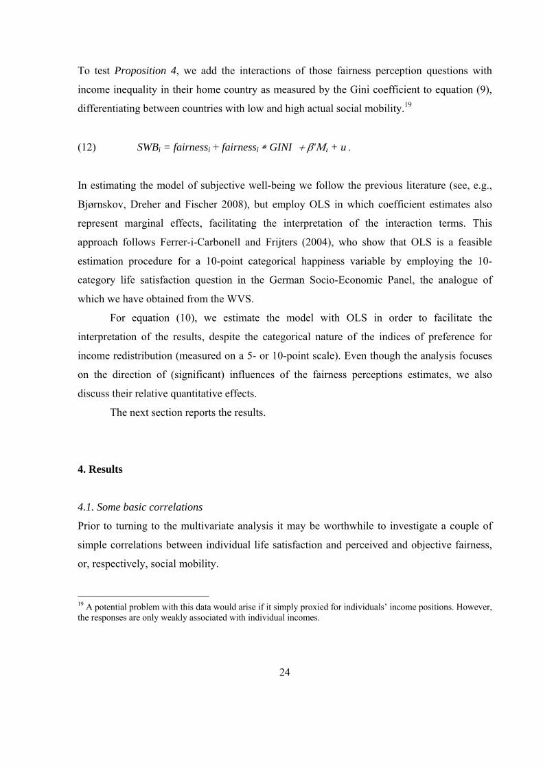
To test Proposition 4, we add the interactions of those fairness perception questions with

income inequality in their home country as measured by the Gini coefficient to equation (9),

differentiating between countries with low and high actual social mobility.19

(12) SWBi = fairnessi + fairnessiGINI '+ u

In estimating the model of subjective well-being we follow the previous literature (see, e.g.,

Bjørnskov, Dreher and Fischer 2008), but employ OLS in which coefficient estimates also

represent marginal effects, facilitating the interpretation of the interaction terms. This

approach follows Ferrer-i-Carbonell and Frijters (2004), who show that OLS is a feasible

estimation procedure for a 10-point categorical happiness variable by employing the 10-

category life satisfaction question in the German Socio-Economic Panel, the analogue of

which we have obtained from the WVS.

For equation (10), we estimate the model with OLS in order to facilitate the

interpretation of the results, despite the categorical nature of the indices of preference for

income redistribution (measured on a 5- or 10-point scale). Even though the analysis focuses

on the direction of (significant) influences of the fairness perceptions estimates, we also

discuss their relative quantitative effects.

The next section reports the results.

4. Results

4.1. Some basic correlations

Prior to turning to the multivariate analysis it may be worthwhile to investigate a couple of

simple correlations between individual life satisfaction and perceived and objective fairness,

or, respectively, social mobility.

19 A potential problem with this data would arise if it simply proxied for individuals’ income positions. However, the responses are only weakly associated with individual incomes.

25

Simple correlations between measures of fairness perceptions and individual life

satisfaction are rather low or moderate, with coefficient values ranging between roughly 0.05

(hard work) and 0.2 (chance to escape poverty). Correlations with measures of real social

mobility are also small. For measures of wage and income persistence across generations they

range from 0.04 for the income elasticity measure by Blanden (2013) to 0.13 for the measure

of female wage persistence across generations in Causa et al. (2009). For measures that relate

educational outcomes across generations, the correlation ranges from -0.07 for the

intergenerational correlation of education from Hertz et al. (2007) to 0.1 for a measure of

persistence in below upper secondary education from Causa et al. (2009), all in absolute

terms. Finally, the correlation between gross income inequality and life satisfaction is

positive, but fairly small (0.15).

In general, correlations of roughly 0.2 to 0.6 are achieved when an aggregate measure

of happiness is employed in place of individual subjective well-being. Using the mean of life

satisfaction in a country, the strength of the link between individual and parental earnings

from D’Addio (2007) shows a correlation of about 0.5, and persistence in wages between 0.32

and 0.59. Measures of educational persistence are correlated with the aggregated measure

between 0.17 and 0.44. The gross Gini coefficients still show a correlation of 0.4 with country

means in life satisfaction. Employing aggregated individual data on the four fairness

perception measures, correlations with country means in life satisfaction range from -0.08 to

0.37 and are, for at least two measures (chance to escape poverty and being politically

conservative), quite large.

4.2. Testing Proposition 1: Fairness perceptions and subjective well-being

Table 2 tests Proposition 1 by including the proxies for perceived fairness to the baseline

specification of the well-being model, one-by-one. Overall, Table 2 tests four fairness

measures, yielding four model variants. The table displays only the estimation results for the

fairness measure and the number of individual observations in the corresponding regression

samples; the full model estimations are displayed in the Appendix (Table A1, columns 2 - 5).

26

The constant in the regressions is in most cases around 8 SWB points (not reported), and the

adjusted R2 ranges between 0.2 and 0.25, depending on the model specification.20

Table 2: Relations between happiness and fairness perceptions

Notes: OLS estimations. Dependent variable is life satisfaction measured on a 10-point scale. Cluster adjusted standard errors in parentheses. All models include the baseline micro-variables, and interacted country- and wave-fixed effects (not reported). Income, education and occupational status are excluded from the model. *, **, *** denote significances at the 10, 5 and 1 percent level, respectively. The countries included in each regression sample are presented in Table D3 of the Appendix.

First, note the positive signs of the perceived-fairness estimates, which indicate that

persons with high fairness perceptions are indeed happier on average. As all four fairness

estimates are significant at the 1 percent level, the results are clearly in line with Proposition

1. The quantitative impact of these variables is considerable, with coefficients ranging

between 0.25 (hard work) and 0.51 (laziness). Comparing these effects with those of other

determinants of subjective well-being as reported in the Appendix (Tables A1 and A2) shows

that these effects are comparable with, for example, taking part in religious service once a

month as compared to never (0.18) or being married as compared to being divorced or

separated (0.67). According to Table A2 in the Appendix, the largest associations of about

half a life satisfaction category are observable for labor market mobility perceptions (‘people

are poor due to laziness’ and ‘people have a chance to escape poverty’) and ‘conservative

ideology’. Further investigation shows that these relative differences across fairness

20 The constant can be interpreted as the baseline SWB level of the reference group, which, in this specification, has low fairness perceptions, is male, has no children, is religious but not affiliated to a major religion, is divorced or separated from her partner, does not believe in a superior being, and never attends religious service.

Dependent variable: Life Satisfaction

(1) (2) (3) (4)

Hard work brings success in the long run 0.248***

[0.017]

People are poor due to laziness, not injustice 0.418***

[0.031]

People have chance to escape poverty 0.510***

[0.056]

Conservative ideology 0.351***

[0.022]

Observations 180,985 136,683 63,880 291,305

R‐squared 0.21 0.24 0.26 0.22

27

perception coefficients are not caused by changes in sample sizes across regressions (not

reported). In summary, our empirical results are in line with Proposition 1, suggesting that

persons who perceive the income generation process as fair experience higher levels of

subjective well-being.

According to our model, perceived social mobility should have a positive impact on

individual human capital investments, expected life-time earnings and occupational status in

equilibrium, with perceived social mobility affecting subjective well-being through these

transmission channels. As our next step, we therefore test the same empirical model

specification, but include measures of education, income, and occupational status. Table 3

reports the results and shows analogously to Table 2 that persons who perceive themselves as

living in a fair society experience higher levels of subjective well-being. In line with our

model, persons with higher income or better education are happier (for full estimation results,

again see the Appendix Table A2). Comparing the fairness perception estimates across

models (Tables 2 and 3), we observe for all four fairness perception measures smaller

coefficient sizes in Table 3, with all differences being statistically significant at the 1 percent

level. Thus, while the fairness measures remain significant and sizable, the SWB effects of

fairness and social mobility perceptions are partly mediated through own human capital

investment. This finding is again in line with our model predictions.

28

Table 3: Relations between happiness and fairness perceptions – testing the transmission channels income, occupation and education

Notes: OLS estimation. Dependent variable is life satisfaction measured on a 10-point scale. Cluster adjusted standard errors in parentheses. All models include the baseline micro-variables, income, education and occupational status, and interacted country- and wave- fixed effects (not reported). *, **, *** denote significances at the 10, 5 and 1 percent level, respectively. The countries included in each regression sample are presented in Table D3 of the Appendix.

4.3. Testing Proposition 2: Fairness perception, demand for redistribution, and subjective

well-being

Table 4 tests the prediction of Proposition 2 that persons who perceive the income generating

process as fair have a lower demand for equalizing the income distribution through

redistribution from the rich to the poor. We estimate OLS models for the four fairness

perception variables employed in the happiness models (Proposition 1) with three categorical

proxies of preference for income redistribution as dependent variables, as described in Table 1

(preference for ‘a more equal income distribution’, for ‘eliminating income inequality’, and

for ‘guaranteeing basic needs’, respectively). Due to missing observations in the regressors

and regressands, not all 3x4 possible combinations could be estimated. Table 4 reports the

coefficient estimates, their level of significance and the number of observations in the

regression samples.

Almost all regressions (but one) in Table 4 suggest that people who perceive the

income generating process as fair favor less redistribution through the government. This is

observable for the measures ‘poverty due to laziness’, ‘chance to escape poverty’ and


(1) (2) (3) (4)

Hard work brings success in the long run 0.224***

[0.016]

People are poor due to laziness, not injustice 0.374***

[0.028]

People have chance to escape poverty 0.460***

[0.058]

Conservative ideology 0.305***

[0.021]

Observations 180,985 136,683 63,880 291,305

R‐squared 0.24 0.26 0.29 0.25

29

‘conservative ideology’. Notably, these individual ideology and perceived fairness effects are,

given that we employ country fixed effects, independent of 'national' beliefs and political

cultures and thus relative to countries’ potentially time-invariant average perceptions. The

marginal effects suggest that having high fairness perceptions decreases the demand for

government activities by up to half a category (out of possible 10 in column 1) or a third of a

category (out of possible 5 in column 2). Thus, the results are in line with Proposition 2,

suggesting that persons who believe in procedural fairness oppose government redistribution.

Table 4: Fairness perceptions and the demand for income redistribution

Notes: OLS estimations. Dependent variable is a 5- or 10-point scale measure of preference for income redistribution. Cluster adjusted standard errors in parentheses. All models include the baseline micro-variables, income, education and occupational status, and interacted country- and wave- fixed effects (not reported). Missing regressions are due to insufficient sample sizes. *, **, *** denote significances at the 10, 5 and 1 percent level, respectively. The countries included in each regression sample are presented in Table D3 of the Appendix.

Somewhat astonishing is the increase in the probability of favoring a more equal

income distribution expressed by persons e.g. who also believe that ‘hard work brings success

in the long run’, possibly reflecting a modern version of Weber’s hypothesis of a Protestant

work ethic, combined with a charitable attitude towards the poor. 21 Arguably, ‘having

success’ is multidimensional, whereas ‘escaping poverty’ is one-dimensionally related to

gaining income only. However, as this variable can only be included in model 1, we cannot

21 In the traditional Calvinist view and according to their predestination theory, only the efforts of the ‘blessed’ would yield economic success, in contrast to that by the ‘lost souls’. Thus, economic success in ‘this world’ is perceived by Calvinists as a signal for being chosen to have a good afterlife.

Coef. Std. err. Coef. Std. err. Coef. Std. err.

Hard work brings success in the long run 0.08** [0.04] ‐ ‐ ‐ ‐

Adj. R‐Squared 0.09 ‐ ‐

Number of observations 188,420 ‐ ‐

People are poor due to laziness, not injustice ‐0.57*** [0.05] ‐0.29*** [0.03] ‐0.03*** [0.01]

Adj. R‐Squared 0.1 0.12 0.96

Number of observations 130,031 31,811 143,516

People have chance to escape poverty ‐0.40*** [0.06] ‐ ‐ ‐ ‐

Adj. R‐Squared 0.08 ‐ ‐

Number of observations 63,111 ‐ ‐

Conservative ideology ‐0.66*** [0.04] ‐0.35*** [0.06] ‐0.01*** [0.01]

Adj. R‐Squared 0.11 0.12 0.90


(1) (2) (3)

Incomes should be more

equal

It is important to eliminate

income inequality

It is important to

guarantee basic needs

30

draw a clear conclusion on whether the positive sign is a statistical artifact or indicates a

generic relation.

Overall, the results in Table 4 support the prediction of Proposition 2 that perceived

social mobility reduces the demand for income redistribution from the rich to the poor. This

result is required as a basis upon which the interpretation of the following results rests.

Table 5 tests the second part of Proposition 2, which predicts a negative relationship

between a preference for redistribution and individual welfare. This prediction translates into

our empirical model based on the WVS that persons with a preference for ‘a more equal

income distribution’, for ‘eliminating income inequality’, or for ‘guaranteeing basic needs’

(see Table 4) should report lower levels of subjective well-being. All three columns of Table

5 indeed show that persons who demand a more equal income distribution (potentially

through government intervention) and guaranteed basic needs for everybody are less satisfied

with their lives compared to those with no such preferences. With coefficient estimates

between -0.14 and -0.24, the quantitative effect on subjective well-being is of medium size,

comparable to that of, for example, 'cohabiting' as opposed to being 'divorced or separated'.

Overall, Tables 4 and 5 present evidence in line with Proposition 2: we find that those

who perceive their society as fair are less likely to demand a more equal (post-tax and

-transfer) income distribution. Furthermore, we also find that those who do demand more

equal incomes report lower levels of life satisfaction.

Table 5: Subjective well-being and the demand for redistribution


(1) (2) (3)

Incomes should be more equal ‐0.218***

[0.021]

It is important to eliminate income inequality ‐0.239***

[0.041]

It is important to guarantee basic needs ‐0.142*

(0.079)

Observations 255,449 38,257 38,782

R‐squared 0.24 0.28 0.28

31


4.4. Propositions 3 and 4: Inequality and fairness perceptions in low and high actual mobility

countries

While Proposition 3 predicts a positive interaction between fairness perceptions and income

inequality on subjective well-being, Proposition 4 makes the seemingly counter-intuitive

prediction that this pattern is stronger in countries with low actual social mobility. We test

these propositions by interacting the individual fairness perception variables with the Gini

coefficient, and subsequently splitting the regression samples by actual social mobility at the

country level. As described above, we employ two sets of social mobility measures: one for

intergenerational income/wage persistence; and one for educational mobility across

generations.

Our theoretical model predicts that in the sample with low actual social mobility, we

should observe a positive interaction between perceived fairness and income inequality. For

countries with high upward mobility, our model theoretically predicts the positive interaction

to become smaller and weaker. We test these predictions in Tables 6 and 7.

32

Table 6: Fairness perception and Income Inequality – low and high intergenerational mobility in income and wages


Table 6 tests Proposition 4 by employing measures of mobility in wages and income while

Table 7 employs measures of mobility in education instead. The model in Tables 6 and 7 and

the empirical corroboration of Proposition 4 hinges on the assumption that social mobility,

educational mobility, and wage mobility are sufficiently correlated. For all fairness perception

measures in Table 6, in low wage or income mobility countries the effect of income inequality

(1) Low (1) Low (1) Low

Coef. Std. err. Coef. Std. err. Coef. Std. err. Coef. Std. err. Coef. Std. err. Coef. Std. err.

Intergenerational earnings elasticity (d'Addio 2007)

Conservative ideology ‐0.13 [0.32] ‐0.24 [0.29] ‐ ‐ ‐ ‐ ‐ ‐ ‐ ‐

Conservative ideology x Income Inequality 0.73 [0.72] 0.91 [0.67] ‐ ‐ ‐ ‐ ‐ ‐ ‐ ‐

Hard work brings success in the long run ‐ ‐ ‐ ‐ ‐0.46 [0.37] 0.96* [0.50] ‐ ‐ ‐ ‐

Hard work x Income Inequality ‐ ‐ ‐ ‐ 1.57* [0.79] ‐1.70 [1.15] ‐ ‐ ‐ ‐

People are poor due to laziness, not injustice ‐ ‐ ‐ ‐ ‐ ‐ ‐ ‐ ‐0.12 [0.34] 0.1 [0.36]

Laziness x Income Inequality ‐ ‐ ‐ ‐ ‐ ‐ ‐ ‐ 0.65 [0.77] 0.34 [0.79]

Adj. R‐Squared 0.09 0.09 0.10 0.08 0.08 0.08

Number of observations 35,928 23,159 25,084 16,917 22,121 10,949

Summary measure of wage persistence, male (Causa et al. 2009)


Conservative ideology x Income Inequality 0.78* [0.37] 0.52 [0.98] ‐ ‐ ‐ ‐ ‐ ‐ ‐ ‐

Hard work brings success in the long run ‐ ‐ ‐ ‐ 0.02 [0.26] 0.73 [0.50] ‐ ‐ ‐ ‐

Hard work x Income Inequality ‐ ‐ ‐ ‐ 0.53 [0.60] ‐1.06 [1.01] ‐ ‐ ‐ ‐

People are poor due to laziness, not injustice ‐ ‐ ‐ ‐ ‐ ‐ ‐ ‐ 0.06 [0.22] ‐0.26 [0.34]


Adj. R‐Squared 0.07 0.11 0.08 0.11 0.07 0.11


Summary measure of wage persistence, female (Causa et al. 2009)


Conservative ideology x Income Inequality 1.01** [0.41] 0.75 [0.91] ‐ ‐ ‐ ‐ ‐ ‐ ‐ ‐

Hard work brings success in the long run ‐ ‐ ‐ ‐ ‐0.11 [0.33] 0.53 [0.40] ‐ ‐ ‐ ‐


People are poor due to laziness, not injustice ‐ ‐ ‐ ‐ ‐ ‐ ‐ ‐ 0.00 [0.24] 0.03 [0.32]


Adj. R‐Squared 0.08 0.10 0.08 0.10 0.08 0.10


Intergenerational income elasticity (Blanden 2013)

Conservative ideology ‐0.96*** [0.24] 0.02 [0.23] ‐ ‐ ‐ ‐ ‐ ‐ ‐ ‐

Conservative ideology x Income Inequality 2.55*** [0.48] 0.30 [0.53] ‐ ‐ ‐ ‐ ‐ ‐ ‐ ‐


Hard work x Income Inequality ‐ ‐ ‐ ‐ 1.23** [0.56] 0.11 [1.31] ‐ ‐ ‐ ‐


Laziness x Income Inequality ‐ ‐ ‐ ‐ ‐ ‐ ‐ ‐ 1.81 [1.10] ‐0.32 [0.68]

Adj. R‐Squared 0.08 0.12 0.08 0.13 0.07 0.13


(1) High (1) High (1) High

33

on subjective well-being is the more positive the higher the individuals’ fairness perceptions

are. In these countries our theory predicts that the pool of high fairness perception individuals

comprises a larger share of high-income people who profit from higher inequality via higher

status utility. Equally in line with Proposition 4, in high actual mobility country samples we

observe only insignificant or weakly significant interactions with inequality. In general, the

regressions that employ measures of educational mobility are also in line with our predictions,

particularly those that employ large regression samples based on ‘conservative ideology’ and

‘hard work brings success’ as measures of fairness perceptions. The interaction in high actual

mobility countries is again in most cases smaller than in countries with low mobility. A

positive sign of the interaction term can be interpreted as an indication that individuals who

have experienced upward social mobility in their family – and believe this to be the result of

fair institutions – would experience an adverse impact of income redistribution on their well-

being. Again, we find support for Proposition 4 for fairness perception measures that are

similar to those employed in previous empirical studies (e.g., Corneo and Gruener, 2002,

Alesina and LaFerrara, 2005).

34

Table 7: Fairness perception and Income Inequality – low and high intergenerational mobility in educational achievements


To summarize, the empirical results are in line with our propositions. Individuals who

perceive their society as unfair are less likely to be satisfied with their lives (Proposition 1),

and are more likely to oppose redistributive government activities (Proposition 2). In

countries with low actual mobility, people with high fairness perceptions are better off, the

Measure of social mobility Level of mobility

(1) Low (1) High (1) Low (1) High (1) Low (1) High


Summary measure of persistence in below upper secondary education (Causa et al. 2009)







Adj. R‐Squared 0.08 0.10 0.08 0.10 0.08 0.10


Summary measure of persistence in tertiary education (Causa et al. 2009)


Conservative ideology x Income Inequality 0.86* [0.46] 0.96 [0.82] ‐ ‐ ‐ ‐ ‐ ‐ ‐ ‐





Adj. R‐Squared 0.09 0.11 0.09 0.10 0.09 0.10


Intergenerational correlation in educational attainment (Hertz et al. 2007)

Conservative ideology ‐0.15 [0.24] 0.60** [0.23] ‐ ‐ ‐ ‐ ‐ ‐ ‐ ‐

Conservative ideology x Income Inequality 0.81 [0.49] ‐0.73 [0.54] ‐ ‐ ‐ ‐ ‐ ‐ ‐ ‐

Hard work brings success in the long run ‐ ‐ ‐ ‐ 0.59*** [0.13] 0.48*** [0.11] ‐ ‐ ‐ ‐

Hard work x Income Inequality ‐ ‐ ‐ ‐ ‐0.78** [0.30] ‐0.58* [0.29] ‐ ‐ ‐ ‐

People are poor due to laziness, not injustice ‐ ‐ ‐ ‐ ‐ ‐ ‐ ‐ ‐0.01 [0.22] 0.66*** [0.21]

Laziness x Income Inequality ‐ ‐ ‐ ‐ ‐ ‐ ‐ ‐ 0.75* [0.42] ‐0.74 [0.46]

Adj. R‐Squared 0.19 0.27 0.15 0.28 0.17 0.28


Mobility in educational level (Chevalier 2004)

Conservative ideology 0.18 [0.32] 0.52* [0.26] ‐ ‐ ‐ ‐ ‐ ‐ ‐ ‐


Hard work brings success in the long run ‐ ‐ ‐ ‐ 0.12 [0.24] 0.56*** [0.10] ‐ ‐ ‐ ‐

Hard work x Income Inequality ‐ ‐ ‐ ‐ 0.31 [0.55] ‐0.72*** [0.24] ‐ ‐ ‐ ‐

People are poor due to laziness, not injustice ‐ ‐ ‐ ‐ ‐ ‐ ‐ ‐ 0.63* [0.32] 0.70** [0.31]

Laziness x Income Inequality ‐ ‐ ‐ ‐ ‐ ‐ ‐ ‐ ‐0.90 [0.68] ‐0.90 [0.70]

Adj. R‐Squared 0.16 0.12 0.15 0.12 0.16 0.12


35

less redistribution takes place: the higher income inequality is, the more positive are the

effects of high fairness perceptions (Proposition 3). In contrast, in high actual mobility

countries, we observe that the pool of people with high fairness perceptions is less likely to

experience a more positive effect of income inequality (Proposition 4). Because these

findings provide an important qualification to some standard results of elementary welfare

economics, we proceed with a short discussion in the concluding section.

5. Conclusions

The empirical literature on the relationship between income inequality and happiness has

yielded ambiguous results. The point of departure of our analysis is the conjecture that one of

the potential reasons for this confusion might be that people evaluate the fairness of the

income distribution (i.e., the distribution generation process) differently, and that these

subjective evaluations eventually affect their subjective well-being. Extending the previous

literature, we also make the case that inequality assessments hinge on whether or not social

mobility expectations meet actual social mobility.

We illustrate the relationship between inequality and subjective well-being in a small

formal model where individual effort and labor market participation depends on subjectively

perceived probabilities of success that, in turn, reflect fairness perceptions: the higher the

perceived fairness of a society, the closer the individually perceived connection between

individual effort and economic outcomes. We therefore in general expect a positive

relationship between perceived fairness and overall well-being, and a negative effect on the

preference for government redistribution. If ex ante fairness perceptions are sufficiently low,

the individual will choose an investment level of zero, and benefit from a reduction of income

inequality through taxes and transfers. We also distinguish between the effects of perceived

and actual fairness. Low or high actual fairness is associated with low or high upward

mobility, respectively. We argue that a status utility implies that in general, individuals with

high fairness perceptions have a more favorable attitude towards income inequality than

individuals with low fairness perceptions. Furthermore, we argue somewhat paradoxically,

36

that this effect is smaller in countries that are characterized by higher objective mobility, as

measured by low levels of observed income inequality. The reason for this is the difference in

the composition of the pool of high fairness individuals: differences between low fairness

perceptions and high actual fairness (mobility) lead to positive surprises for individuals who

have invested relatively little effort. Thus, in actually fair (mobile) societies the pool of

individuals with high ex post fairness perceptions comprises a larger share of people with

relatively low incomes, who do not profit from status utility. In low fairness (mobility)

countries, the pool comprises a larger share of high-income people who profit to a larger

extent from status utility when income inequality is higher.

We test this model using combined individual-level data of the pooled second to fifth

waves of the World Values Survey (1990-2008), containing about 300,000 interviewed

individuals in 80 countries. According to the results, the respondents’ belief that income

inequality in their society is the result of a comparably fair market process makes them

considerably more satisfied with their lives, while a demand for more government

redistribution for correcting the market-income distribution is negatively associated with

happiness. However, differentiating by level of actual social mobility in a country, in

countries with lower upward-mobility we find evidence for a positive effect of inequality for

individuals with high fairness perceptions, in line with our theoretical prediction. In contrast,

in countries with plenty of economic opportunities and equal chances to success, this positive

interaction effect is either smaller or disappears, depending on the mobility measure used.

The findings challenge the standard Lerner argument that more redistribution and less

income inequality unambiguously leads to an increase in welfare of the average person, and

thus, in average welfare. Instead, the model and the empirical analysis suggest that for broad

groups of countries the potential effects of inequality depend on the interplay between

perceived and actual fairness of the institutional framework. The overall effect of reductions

of inequality on subjective well-being is thus much more ambiguous at the aggregate level of

society than predicted by many standard models. As such, our findings may hold implications

for both policy making and future theorizing on the subject.

37

By keeping our framework relatively simple, we implicitly leave several questions for

future research. A possible extension of our framework would be to look at updating fairness

perceptions in the long run, possibly across generations. If there is long-term convergence of

beliefs to objective fairness, then the disappointment of erring individuals underlying

Proposition 4 would disappear in the long run, as low-fairness individuals subsequently

realize that they actually live in a high-fairness society.

It seems beneficial to overall welfare that governments should not only provide

policies and institutions that guarantee social mobility, but also communicate these policies

convincingly, so that individuals can choose their effort levels accordingly. Individuals who

believe in the fairness of the market-income-generation-process experience a higher

subjective well-being. Thus, policies should aim at fostering competition, reducing privileges

of interest groups and closing the gap between individual effort and success. Inequality is

easier to accept if it is the result of unequally distributed skills and chosen effort levels than if

it is due to institutional design and low social mobility.

Our results suggest that creating a society with such equal opportunities would be

superior with regard to fostering higher subjective well-being to a paternalistic and overly

redistributive welfare state.

38

References

Akerlof, G.A. and R.E. Kranton, 2000, Economics and Identity, Quarterly Journal of

Economics 115: 715-750.

Alesina, A., R. DiTella and R. MacCulloch, 2004, Inequality and Happiness: Are Europeans

and Americans Different? Journal of Public Economics 88: 2009-2042.

Alesina, A. and E. La Ferrara, 2005, Preferences for redistribution in the land of

opportunities, Journal of Public Economics 89: 897-931.

Bergh, A., 2005, On the Counterfactual Problem of Welfare State Research: How Can We

Measure Redistribution? European Sociological Review 21, 4: 345-357.

Bjørnskov, C., A. Dreher and J.A.V. Fischer, 2008, Cross-country determinants of life

satisfaction: Exploring different determinants across groups in society, Social Choice

and Welfare 30: 119-173.

Bjørnskov, C., A. Dreher, J.A.V. Fischer, and J. Schnellenbach, 2010, Inequality and

Happiness: When perceived social mobility and economic reality do not match,

CESifo working paper no. 3216.

Blanchflower, D.G. and A.J. Oswald, 2004, Well-Being Over Time in Britain and the USA,

Journal of Public Economics 88: 1359-1386.

Blanden, J., 2011, Cross-Country Rankings in intergenerational mobility: a comparison of

approaches from economics and sociology, Journal of Economic Surveys 27, 1: 38-73.

Casey, T. and C. Dustmann, 2010, Immigrants' Identity, Economic Outcomes and the

Transmission of Identity Across Generations, Economic Journal 120: F31-F51.

Cahill, M., 2005. Is the Human Development Index Redundant? Eastern Economic Journal

31: 1-5.

Causa, O. and C. Chapuis, 2009, Equity in Student Achievement Across OECD Countries: An

Investigation of the Role of Policies, OECD Economics Department Working Papers,

No. 708.

Causa, O., S. Dantan and Å. Johansson, 2009,. Intergenerational social mobility in European

OECD countries, OECD Economics Department Working Papers, No. 709.

39

Chevalier, A., K. Denny and D. McMahon, 2009, Intergenerational mobility and education

equality. In P. Dolton, R. Asplund and E. Barth (eds.), Education and Inequality

across Europe (pp. 260-281). London:Edward Elgar.

Clark, A.E., P. Frijters and M. Shields, 2008, Relative Income, Happiness, and Utility: An

Explanation for the Easterlin and Other Puzzles, Journal of Economic Literature 46:

95-144.

Clark, A. and E. D’Angelo, 2008, Upward Social Mobility, Wellbeing and Political

Preferences: Evidence from the BHPS, working paper, Paris School of Economics 17.

Corak, M., 2006, Do Poor Children Become Poor Adults? Lessons from a Cross Country

Comparison of Generational Earnings Mobility, IZA Discussion Paper No. 1993.

Corneo, G. and H.P. Gruener, 2002, Individual preferences for political redistribution,

Journal of Public Economics 83: 83-107.

D’Addio, A., 2007, Intergenerational Transmission of Disadvantage: Mobility or Immobility

Across Generations? A Review of the Evidence for OECD countries, OECD Social,

Employment and Migration Working Paper, No. 52.

Deininger, K., and L. Squire, 1996, A New Data Set Measuring Income Inequality, World

Bank Economic Review 10: 565-569.

Diener, E., R.E. Lucas, U. Schimmack and J. Helliwell, 2008, Well-Being for Public Policy,

Oxford, UK: Oxford University Press.

Dohmen, Th., A. Falk, D. Huffman, F. Marklein and U. Sunde, 2009, Biased Probability

Judgment: Evidence of Incidence and Relationship to Economic Outcomes from a

Representative Sample, Journal of Behavioral Organization 72: 903-915.

Ederer, F. and A. Patacconi, 2010, Interpersonal comparison, status and ambition in

organizations, Journal of Economic Behavior and Organization 75: 348-363.

Fehr, E. and K.M. Schmidt, 1999, A theory of fairness, competition, and cooperation,

Quarterly Journal of Economics 114: 817-868.

Ferrer-i-Carbonell, A. and P. Frijters, 2004, How Important is Methodology for the Estimates

of the Determinants of Happiness? The Economic Journal 114: 641-659.

40

Fischer, J.A.V., 2009a. Subjective Well-Being as Welfare Measure: Concepts and

Methodology, MPRA Paper 16619, University Library of Munich, Germany.

Fischer, J.A.V., 2009b, The Welfare Effects of Social Mobility, OECD Social, Employment

and Migration Working Papers 93, OECD, Directorate for Employment, Labour and

Social Affairs.

Fischer, J.A.V., 2009c, Happiness and Age Cycles – Return to Start...?: On the Functional

Relationship between Subjective Well-being and Age, OECD Social, Employment and

Migration Working Papers 99, OECD, Directorate for Employment, Labour and

Social Affairs.

Fischer, J.A.V. and B. Torgler, 2013, Do Positional Concerns Destroy Social Capital:

Evidence from 26 Countries, Economic Inquiry, forthcoming.

Frey, B. and A. Stutzer, 2005, Beyond outcomes: measuring procedural utility, Oxford

Economic Papers 57: 90-111.

Georgiadis, A. and A. Manning, 2012, One nation under a groove? Understanding national

identity, Journal of Economic Behavior and Organization, forthcoming,

http://dx.doi.org/10.1016/j.jebo.2012.10.013.

Grosfeld I. and C. Senik, 2009, The emerging aversion to inequality - Evidence from long

subjective data, PSE Working Papers 2008-19, PSE (Ecole normale supérieure).

Harms, P. and S. Zink, 2003, Limits to Redistribution in a Democracy: A Survey, European

Journal of Political Economy 19: 651-668.

Hayek, F.A., 1944, The Road to Serfdom, Chicago: University of Chicago Press.

Hertz, T., T. Jayasundera, P. Piraino, S. Selcuk, N. Smith and A. Verashchagina, 2007, The

inheritance of educational inequality: international comparisons and fifty-year trends.

The B.E. Journal of Economic Analysis and Policy 7(2).

Hopkins, E., 2008, Inequality, Happiness and Relative Concerns: What Actually is their

Relationship? Journal of Economic Inequality 6: 351-372.

Hirschman, A. and M. Rothschild, 1973, The changing tolerance for income inequality in the

course of economic development, Quarterly Journal of Economics 87: 544-566.

41

Inglehart, R., M. Basañez, J. Díez-Medrano, L. Halman and R. Luijkx, 2004, Human Beliefs

and Values, Ann Arbor: University of Michigan Press.

Layard, R., G. Mayraz and S. Nickell, 2009, Does Relative Income Matter? Are the Critics

Right? CEP Discussion Paper No 918, March 2009.

Lerner, A., 1944, The economics of control: principles of welfare economics, New York:

MacMillan.

Luttmer, E.F.P., 2005, Neighbors as negatives: Relative earnings and well-being, Quarterly

Journal of Economics 120: 963-1002.

Mitchell, G., P.E. Tetlock, B.A. Mellers and L.D. Ordóñez, 1993, Judgments of social justice:

compromises between equality and efficiency, Journal of Personality and Social

Psychology 65: 629-639.

Piketty, T., 1995, Social Mobility and Redistributive Politics, Quarterly Journal of Economics

110: 551-584.

Ravallion, M. and M. Lokshin, 2000, Who wants to redistribute? The tunnel effect in 1990s

Russia, Journal of Public Economics 76: 87-104.

Scott, J.T., R.E. Matland, P.A. Michelbach and B.H. Bornstein, 2001, Just deserts: an

experimental study of distributive justice norms, American Journal of Political

Science 45: 74-767.

Solt, F., 2009, Standardizing the World Income Inequality Database, Social Science Quarterly

90(2): 231-242. SWIID Version 3.1, December 2011.

Stutzer, A., and B.S. Frey, 2003, Institutions Matter for Procedural Utility: An Economic

Study of the Impact of Political Participation Possibilities, in: R. Mudambi et al.

(eds.), Economic Welfare, International Business and Global Institutional Change,

Edward Elgar, Cheltenham, 81-99.

Veblen, T., 1899, The Theory of the Leisure Class, New York: MacMillan.

Veenhoven, R., 2000, The four qualities of life: Ordering concepts and measures of the good

life, Journal of Happiness Studies 1: 1-39.

APPENDIX

Appendix A: Complete estimations for table 2 and 3, ordered probit model for table 4.

A.1. Complete baseline model; fairness perceptions and life satisfaction

(Table 2 in the main text)


(1) (2) (3) (4)

age ‐0.1000*** ‐0.107*** ‐0.132*** ‐0.112***

(0.0183) (0.0230) (0.0316) (0.0143)

age_s 0.164*** 0.179*** 0.223*** 0.190***

(0.0373) (0.0470) (0.0642) (0.0294)

age_3 ‐0.0820*** ‐0.0919*** ‐0.110*** ‐0.0987***

(0.0227) (0.0285) (0.0401) (0.0181)

male ‐0.00898 ‐7.31e‐05 ‐0.0174 ‐0.0470*

(0.0205) (0.0260) (0.0347) (0.0245)

buddhist 0.256*** 0.270 0.504** 0.177***

(0.0876) (0.164) (0.228) (0.0672)

muslim ‐0.0635 ‐0.0680 ‐0.00893 ‐0.0213

(0.0953) (0.190) (0.241) (0.0809)

catholic 0.136*** 0.0947 0.203 0.0968**

(0.0481) (0.0936) (0.155) (0.0436)

protestant 0.213*** 0.210** 0.309* 0.200***

(0.0458) (0.0886) (0.164) (0.0420)

orthodox ‐0.135** ‐0.200* ‐0.129 ‐0.131**

(0.0657) (0.113) (0.196) (0.0572)

other_christ 0.240*** 0.255* 0.528*** 0.0582

(0.0909) (0.136) (0.185) (0.146)

no_rel 0.0857* 0.0987 0.189 0.0580

(0.0507) (0.0985) (0.165) (0.0467)

jewish ‐0.0861 ‐0.0617 0.140 ‐0.0526

(0.163) (0.226) (0.268) (0.121)

hindu 0.200 0.258 0.438 0.197*

(0.158) (0.274) (0.378) (0.119)

age_Kat2 ‐0.00827 ‐0.0250 ‐0.0350 0.0170

(0.0411) (0.0484) (0.0799) (0.0303)

age_Kat3 ‐0.0320 ‐0.0863 ‐0.0818 0.00825

(0.0582) (0.0682) (0.115) (0.0436)

age_Kat4 ‐0.0868 ‐0.145* ‐0.101 ‐0.0664

(0.0686) (0.0836) (0.135) (0.0538)

2

age_Kat5 ‐0.0589 ‐0.107 ‐0.180 ‐0.0602

(0.0922) (0.108) (0.154) (0.0700)

age_Kat6 ‐0.131 ‐0.135 ‐0.298* ‐0.116

(0.103) (0.123) (0.173) (0.0805)

single_f 0.192*** 0.269*** 0.206*** 0.185***

(0.0425) (0.0456) (0.0680) (0.0364)

single_m 0.189*** 0.229*** 0.241*** 0.157***

(0.0451) (0.0502) (0.0783) (0.0412)

married 0.675*** 0.735*** 0.743*** 0.659***

(0.0276) (0.0264) (0.0452) (0.0261)

cohab 0.402*** 0.399*** 0.383*** 0.357***

(0.0512) (0.0599) (0.0844) (0.0455)

prev_child1 ‐0.0831*** ‐0.0545* ‐0.0972** ‐0.116***

(0.0274) (0.0307) (0.0470) (0.0265)

prev_child2 ‐0.0918*** ‐0.0166 ‐0.102* ‐0.0960***

(0.0299) (0.0314) (0.0523) (0.0277)

prev_child3 ‐0.136*** ‐0.0778** ‐0.100 ‐0.151***

(0.0359) (0.0380) (0.0667) (0.0334)

rel_att1 0.463*** 0.489*** 0.457*** 0.377***

(0.0421) (0.0537) (0.0632) (0.0488)

rel_att2 0.282*** 0.282*** 0.235*** 0.217***

(0.0391) (0.0412) (0.0603) (0.0414)

rel_att3 0.164*** 0.193*** 0.126** 0.120***

(0.0369) (0.0365) (0.0581) (0.0330)

rel_att4 0.141*** 0.152*** 0.118** 0.119***

(0.0306) (0.0348) (0.0542) (0.0264)

rel_att5 0.0866* 0.160*** 0.105***

(0.0471) (0.0419) (0.0389)

rel_att6 0.0792*** 0.0756** 0.112** 0.0497*

(0.0287) (0.0314) (0.0479) (0.0280)

rel_att7 0.0224 0.0144 ‐0.0607 ‐0.000348

(0.0312) (0.0306) (0.0460) (0.0270)

belief_sup 0.107*** 0.118*** 0.127*** 0.0858***

(0.0317) (0.0269) (0.0423) (0.0277)

conservative2 0.351***

(0.0224)

hardwork1 0.248***

(0.0172)

laziness3 0.418***

(0.0315)

chance 0.510***

3

(0.0564)

Constant 9.012*** 8.971*** 8.267*** 9.328***

(0.262) (0.324) (0.444) (0.209)

Observations 180,985 136,683 63,880 291,305

R‐squared 0.210 0.239 0.261 0.219

Notes: OLS estimation. Dependent variable is life satisfaction measured on a 10-point scale. Cluster adjusted standard errors in parentheses. All models include the baseline micro-variables, and interactive country-wave effects (not reported). Income, education and occupational status are excluded from the model. *, **, *** denote significances at the 10, 5 and 1 percent level, respectively.

4

A.2. Complete extended model - fairness perceptions, income, education, occupational

status included (Table 3 in the main paper)


(1) (2) (3) (4)

age ‐0.114*** ‐0.125*** ‐0.150*** ‐0.129***

(0.0188) (0.0230) (0.0319) (0.0144)

age_s 0.195*** 0.220*** 0.261*** 0.226***

(0.0384) (0.0469) (0.0657) (0.0297)

age_3 ‐0.0980*** ‐0.115*** ‐0.130*** ‐0.118***

(0.0233) (0.0283) (0.0410) (0.0183)

male ‐0.0287 ‐0.0161 ‐0.0326 ‐0.0512**

(0.0199) (0.0255) (0.0381) (0.0206)

buddhist 0.240*** 0.199 0.384* 0.162**

(0.0824) (0.149) (0.207) (0.0627)

muslim 0.0329 0.0289 0.0737 0.0576

(0.0803) (0.156) (0.192) (0.0720)

catholic 0.102** 0.0336 0.109 0.0564

(0.0427) (0.0821) (0.126) (0.0394)

protestant 0.170*** 0.145* 0.212* 0.148***

(0.0374) (0.0734) (0.121) (0.0353)

orthodox ‐0.135** ‐0.224** ‐0.187 ‐0.139***

(0.0589) (0.0983) (0.159) (0.0513)

other_christ 0.269*** 0.200* 0.419*** 0.111

(0.0633) (0.119) (0.148) (0.113)

no_rel 0.0544 0.0353 0.0883 0.0180

(0.0452) (0.0845) (0.131) (0.0426)

jewish ‐0.227 ‐0.203 ‐0.0493 ‐0.186

(0.175) (0.232) (0.278) (0.123)

hindu 0.211* 0.218 0.379 0.192**

(0.126) (0.210) (0.276) (0.0922)

age_Kat2 0.00807 ‐0.00945 ‐0.0207 0.0310

(0.0385) (0.0460) (0.0701) (0.0289)

age_Kat3 ‐0.0443 ‐0.105 ‐0.0984 ‐0.00505

(0.0554) (0.0647) (0.102) (0.0421)

age_Kat4 ‐0.114* ‐0.183** ‐0.126 ‐0.0910*

(0.0664) (0.0817) (0.126) (0.0526)

age_Kat5 ‐0.0308 ‐0.0755 ‐0.130 ‐0.0280

(0.0877) (0.103) (0.143) (0.0670)

age_Kat6 ‐0.0191 ‐0.0280 ‐0.164 ‐0.00473

(0.0978) (0.117) (0.166) (0.0775)

5

inc_cat2 0.237*** 0.257*** 0.270** 0.239***

(0.0626) (0.0734) (0.131) (0.0448)

inc_cat3 0.413*** 0.430*** 0.403** 0.417***

(0.0792) (0.0895) (0.169) (0.0568)

inc_cat4 0.603*** 0.605*** 0.587*** 0.627***

(0.0857) (0.0894) (0.171) (0.0602)

inc_cat5 0.802*** 0.721*** 0.754*** 0.815***

(0.0989) (0.0984) (0.177) (0.0710)

inc_cat6 0.936*** 0.801*** 0.803*** 0.951***

(0.0996) (0.0981) (0.175) (0.0728)

inc_cat7 1.105*** 0.919*** 0.970*** 1.105***

(0.105) (0.100) (0.182) (0.0766)

inc_cat8 1.215*** 0.985*** 1.071*** 1.195***

(0.111) (0.101) (0.181) (0.0823)

inc_cat9 1.208*** 1.081*** 1.180*** 1.227***

(0.107) (0.102) (0.187) (0.0823)

inc_cat10 1.314*** 1.199*** 1.318*** 1.297***

(0.109) (0.102) (0.184) (0.0832)

inc_cat11 0.713*** 0.661*** 0.678*** 0.749***

(0.0808) (0.0832) (0.146) (0.0605)

edu_cat2 0.230*** 0.234*** 0.317** 0.129***

(0.0594) (0.0849) (0.124) (0.0480)

edu_cat3 0.275*** 0.259** 0.334* 0.205***

(0.0740) (0.106) (0.167) (0.0570)

edu_cat4 0.401*** 0.405*** 0.519*** 0.284***

(0.0705) (0.102) (0.150) (0.0591)

edu_cat5 0.288*** 0.334*** 0.364** 0.208***

(0.0828) (0.110) (0.168) (0.0617)

edu_cat6 0.415*** 0.450*** 0.554*** 0.299***

(0.0770) (0.109) (0.164) (0.0631)

edu_cat7 0.428*** 0.478*** 0.496*** 0.342***

(0.0784) (0.112) (0.158) (0.0653)

edu_cat8 0.561*** 0.626*** 0.706*** 0.440***

(0.0816) (0.121) (0.175) (0.0700)

edu_cat9 0.288** 0.334* 0.501* 0.247**

(0.129) (0.172) (0.264) (0.106)

single_f 0.102*** 0.178*** 0.0996* 0.0876**

(0.0378) (0.0403) (0.0581) (0.0367)

single_m 0.120*** 0.170*** 0.169** 0.0726

(0.0410) (0.0452) (0.0670) (0.0450)

married 0.488*** 0.556*** 0.559*** 0.461***

6

(0.0329) (0.0295) (0.0512) (0.0283)

cohab 0.314*** 0.345*** 0.345*** 0.269***

(0.0464) (0.0562) (0.0797) (0.0415)

prev_child1 ‐0.0414* ‐0.0257 ‐0.0650 ‐0.0806***

(0.0239) (0.0280) (0.0426) (0.0293)

prev_child2 ‐0.0538* 0.00615 ‐0.0696 ‐0.0680**

(0.0277) (0.0303) (0.0544) (0.0308)

prev_child3 ‐0.0179 0.0143 0.0229 ‐0.0471

(0.0307) (0.0343) (0.0588) (0.0365)

self_empl 0.0397 0.0424 0.0487 0.0172

(0.0294) (0.0354) (0.0644) (0.0263)

housewife 0.0622 0.0391 0.0783 0.0787**

(0.0378) (0.0408) (0.0664) (0.0345)

retired ‐0.0819** ‐0.117*** ‐0.0949 ‐0.107***

(0.0373) (0.0415) (0.0647) (0.0310)

other ‐0.110* ‐0.153** ‐0.00155 ‐0.116***

(0.0585) (0.0594) (0.0846) (0.0439)

student 0.0700* 0.0625 0.0858 0.0277

(0.0371) (0.0422) (0.0631) (0.0283)

unempl_indi ‐0.465*** ‐0.613*** ‐0.495*** ‐0.521***

(0.0481) (0.0584) (0.0800) (0.0392)

rel_att1 0.446*** 0.476*** 0.456*** 0.378***

(0.0415) (0.0519) (0.0603) (0.0437)

rel_att2 0.262*** 0.262*** 0.226*** 0.211***

(0.0376) (0.0370) (0.0532) (0.0371)

rel_att3 0.143*** 0.168*** 0.122** 0.111***

(0.0365) (0.0349) (0.0554) (0.0310)

rel_att4 0.119*** 0.126*** 0.111** 0.104***

(0.0306) (0.0344) (0.0542) (0.0258)

rel_att5 0.0794 0.142*** 0.0980**

(0.0492) (0.0401) (0.0390)

rel_att6 0.0605** 0.0477* 0.0974** 0.0339

(0.0272) (0.0287) (0.0440) (0.0266)

rel_att7 0.0184 0.00510 ‐0.0497 ‐0.00139

(0.0300) (0.0284) (0.0430) (0.0249)

belief_sup 0.157*** 0.159*** 0.181*** 0.118***

(0.0306) (0.0260) (0.0383) (0.0335)

conservative2 0.305***

(0.0209)

hardwork1 0.224***

(0.0162)

7

Fcowave132 1.057***

(0.133)

laziness3 0.374***

(0.0283)

chance 0.460***

(0.0582)

Constant 8.280*** 7.296*** 6.839*** 8.688***

(0.296) (0.334) (0.559) (0.237)

Observations 180,985 136,683 63,880 291,305

R‐squared 0.239 0.262 0.288 0.247

Notes: OLS estimation. Dependent variable is life satisfaction measured on a 10-point scale. Cluster adjusted standard errors in parentheses. All models include the baseline micro-variables, income, education and occupational status, and interactive country-wave effects (not reported). *, **, *** denote significances at the 10, 5 and 1 percent level, respectively.

8

A.3. Table A3: Fairness perceptions and the demand for income redistribution

(Table 4 in the main paper with ordered probit estimation)

Coef. Std. err.

Hard work brings success in the long run ‐0.04*** [0.01]

Number of observations 188,420

People are poor due to laziness, not injustice ‐0.20*** [0.02] ‐0.29*** [0.03] ‐0.22*** [0.03]


People have chance to escape poverty ‐0.14*** [0.02]

Number of observations 63111

Conservative ideology ‐0.23*** [0.02] ‐0.33*** [0.05] ‐0.14*** [0.03]


Incomes should be more

equal

Important to eliminate

income inequality

Importance of

guaranteeing basic

needs

(1) (2) (3)

Ordered probit estimations. Dependent variable is a 5- or 10-point scale measure of preference for income redistribution. Cluster adjusted standard errors in parentheses. All models include the baseline micro-variables, income, education and occupational status, and interactive country-wave effects (not reported). Missing regressions are due to insufficient sample sizes. *, **, *** denote significances at the 10, 5 and 1 percent level, respectively.

Guideline Appendix B and C: In the following alternative specifications of table 6 and 7 in the main paper are presented as robustness checks. The first specification is a fully interacted model, the second includes our first optimism questions additionally, the third includes our second optimism measure and the fourth tests our assumptions for employed people only.

9

B. Robustness check related to table 6: Fairness perception and Income Inequality- low and

high mobility in income and wages

B.1. Fully interacted model

Measure of social mobility(1) Low (1) Low



Hard work x Income Inequality 22.15*** [4.08] ‐ ‐ ‐ ‐

Hard work x Income Inequality x Mobility ‐31.96*** [5.80] ‐ ‐ ‐ ‐

Laziness x Income Inequality ‐ ‐ 10.85** [5.32] ‐ ‐

Laziness x Income Inequality x Mobility ‐ ‐ ‐13.05* [7.51] ‐ ‐

Conservative ideology x Income Inequality ‐ ‐ ‐ ‐ ‐6.66 [4.50]

Conservative ideology x Income Inequality x Mobility ‐ ‐ ‐ ‐ 11.34* [6.29]

Adj. R‐Squared 0.02 0.01 0.01



Hard work x Income Inequality 2.30 [1.93] ‐ ‐ ‐ ‐

Hard work x Income Inequality x Mobility ‐3.37 [3.22] ‐ ‐ ‐ ‐

Laziness x Income Inequality ‐ ‐ ‐1.30 [1.68] ‐ ‐

Laziness x Income Inequality x Mobility ‐ ‐ 2.79 [2.86] ‐ ‐

Conservative ideology x Income Inequality ‐ ‐ ‐ ‐ 1.01 [1.80]

Conservative ideology x Income Inequality x Mobility ‐ ‐ ‐ ‐ ‐1.02 [3.04]

Adj. R‐Squared 0.01 0.01 0.01


Summary measure of wage persistence, female (Causa et al.2009)



Laziness x Income Inequality ‐ ‐ 1.60 [1.27] ‐ ‐

Laziness x Income Inequality x Mobility ‐ ‐ ‐1.80 [2.13] ‐ ‐


Conservative ideology x Income Inequality x Mobility ‐ ‐ ‐ ‐ 0.81 [2.11]

Adj. R‐Squared 0.03 0.02 0.02



Hard work x Income Inequality ‐3.3 [2.53] ‐ ‐ ‐ ‐

Hard work x Income Inequality x Mobility 3.28 [3.76] ‐ ‐ ‐ ‐



Conservative ideology x Income Inequality ‐ ‐ ‐ ‐ ‐3.68 [2.56]

Conservative ideology x Income Inequality x Mobility ‐ ‐ ‐ ‐ 7.84** [3.80]

Adj. R‐Squared 0.01 0.01 0.01


Level of mobility(1) High


10

B.2. Identical to table 6 in the main paper, only focusing on the 1990 wave including a

measure of optimism ( "I am good at getting what I want")


(1) Low (1) Low (1) Low



Conservative ideology ‐0.63 [0.50] ‐0.52** [0.18] ‐ ‐ ‐ ‐ ‐ ‐ ‐ ‐

Conservative ideology x Income Inequality 1.84 [1.12] 1.45** [0.41] ‐ ‐ ‐ ‐ ‐ ‐ ‐ ‐

Hard work brings success in the long run ‐ ‐ ‐ ‐ ‐0.12 [0.27] 1.89*** [0.28] ‐ ‐ ‐ ‐

Hard work x Income Inequality ‐ ‐ ‐ ‐ 0.82 [0.66] ‐4.00*** [0.69] ‐ ‐ ‐ ‐



Adj. R‐Squared 0.08 0.06 0.08 0.07 0.08 0.07

Number of observations 13768 5439 13227 5273 11916 4378





Hard work x Income Inequality ‐ ‐ ‐ ‐ 0.81* [0.34] ‐1.91 [1.12] ‐ ‐ ‐ ‐

People are poor due to laziness, not injustice ‐ ‐ ‐ ‐ ‐ ‐ ‐ ‐ ‐0.22 [0.16] ‐0.13 [0.51]

Laziness x Income Inequality ‐ ‐ ‐ ‐ ‐ ‐ ‐ ‐ 1.10** [0.41] 0.66 [1.00]

Adj. R‐Squared 0.07 0.11 0.07 0.11 0.07 0.11









Adj. R‐Squared 0.07 0.1 0.08 0.1 0.07 0.1



Conservative ideology ‐0.90* [0.36] ‐0.65* [0.25] ‐ ‐ ‐ ‐ ‐ ‐ ‐ ‐

Conservative ideology x Income Inequality 2.34** [0.66] 1.81** [0.60] ‐ ‐ ‐ ‐ ‐ ‐ ‐ ‐

Hard work brings success in the long run ‐ ‐ ‐ ‐ ‐0.61** [0.21] 1.70** [0.40] ‐ ‐ ‐ ‐

Hard work x Income Inequality ‐ ‐ ‐ ‐ 1.91*** [0.45] ‐3.45** [0.93] ‐ ‐ ‐ ‐


Laziness x Income Inequality ‐ ‐ ‐ ‐ ‐ ‐ ‐ ‐ 0.92* [0.37] 0.2 [0.96]

Adj. R‐Squared 0.07 0.12 0.07 0.13 0.07 0.13




11

B.3. Identical to table 6 in the main paper, only focusing on the 1990 wave including

another measure of optimism ( " I usually count on being successful in everything I

do")


(1) Low (1) Low (1) Low





Hard work brings success in the long run ‐ ‐ ‐ ‐ ‐0.11 [0.25] 1.90*** [0.38] ‐ ‐ ‐ ‐

Hard work x Income Inequality ‐ ‐ ‐ ‐ 0.80 [0.63] ‐3.99** [0.92] ‐ ‐ ‐ ‐



Adj. R‐Squared 0.08 0.06 0.08 0.06 0.08 0.06



Conservative ideology ‐0.18 [0.19] 0.12 [0.68] ‐ ‐ ‐ ‐ ‐ ‐ ‐ ‐



Hard work x Income Inequality ‐ ‐ ‐ ‐ 0.84** [0.31] ‐1.97 [1.23] ‐ ‐ ‐ ‐


Laziness x Income Inequality ‐ ‐ ‐ ‐ ‐ ‐ ‐ ‐ 1.11* [0.47] 0.74 [1.30]

Adj. R‐Squared 0.06 0.11 0.07 0.11 0.07 0.11




Conservative ideology x Income Inequality 1 [0.76] 0.6 [1.29] ‐ ‐ ‐ ‐ ‐ ‐ ‐ ‐





Adj. R‐Squared 0.07 0.10 0.08 0.10 0.07 0.10



Conservative ideology ‐1.02** [0.37] ‐0.36* [0.16] ‐ ‐ ‐ ‐ ‐ ‐ ‐ ‐

Conservative ideology x Income Inequality 2.60** [0.70] 1.18** [0.38] ‐ ‐ ‐ ‐ ‐ ‐ ‐ ‐

Hard work brings success in the long run ‐ ‐ ‐ ‐ ‐0.65** [0.20] 1.74** [0.51] ‐ ‐ ‐ ‐

Hard work x Income Inequality ‐ ‐ ‐ ‐ 2.01*** [0.44] ‐3.50** [1.16] ‐ ‐ ‐ ‐


Laziness x Income Inequality ‐ ‐ ‐ ‐ ‐ ‐ ‐ ‐ 0.99** [0.36] 0.06 [1.33]

Adj. R‐Squared 0.07 0.13 0.07 0.13 0.07 0.13




12

B.4. Identical to table 6 in the main paper, only focusing on employed people.


(1) Low (1) Low (1) Low





Hard work brings success in the long run ‐ ‐ ‐ ‐ ‐0.44 [0.32] 1.12** [0.49] ‐ ‐ ‐ ‐

Hard work x Income Inequality ‐ ‐ ‐ ‐ 1.52** [0.69] ‐2.06* [1.13] ‐ ‐ ‐ ‐



Adj. R‐Squared 0.07 0.07 0.08 0.07 0.06 0.07









Adj. R‐Squared 0.07 0.10 0.07 0.10 0.06 0.10



Conservative ideology ‐0.29* [0.15] ‐0.27 [0.45] ‐ ‐ ‐ ‐ ‐ ‐ ‐ ‐






Adj. R‐Squared 0.07 0.09 0.07 0.09 0.07 0.08



Conservative ideology ‐1.03*** [0.24] 0.05 [0.28] ‐ ‐ ‐ ‐ ‐ ‐ ‐ ‐

Conservative ideology x Income Inequality 2.72*** [0.49] 0.26 [0.63] ‐ ‐ ‐ ‐ ‐ ‐ ‐ ‐



People are poor due to laziness, not injustice ‐ ‐ ‐ ‐ ‐ ‐ ‐ ‐ ‐0.49 [0.43] 0.84* [0.41]


Adj. R‐Squared 0.07 0.09 0.07 0.10 0.06 0.09




13

C. Robustness check related to table 7: Fairness perception and Income Inequality- low and

high mobility in educational achievements.

C.1. Fully interacted model

Table 7: Fairness perception and Income Inequality - low and high mobility in educational achievements

Measure of social mobility

(1) Low (1) High (1) Low






Laziness x Income Inequality x Mobility ‐ ‐ 0.03 [3.25] ‐ ‐



Adj. R‐Squared 0.10 0.10 0.10







Conservative ideology x Income Inequality ‐ ‐ ‐ ‐ 4.22* [2.12]


Adj. R‐Squared 0.10 0.10 0.10


Intergenerational correlation in educational attainment (Hertz et al. (2007)





Conservative ideology x Income Inequality ‐ ‐ ‐ ‐ 5.54*** [1.61]

Conservative ideology x Income Inequality x Mobility ‐ ‐ ‐ ‐ ‐9.41*** [2.76]

Adj. R‐Squared 0.22 0.24 0.22






Laziness x Income Inequality x Mobility ‐ ‐ ‐0.12** [0.06] ‐ ‐

Conservative ideology x Income Inequality ‐ ‐ ‐ ‐ 2.26* [1.13]

Conservative ideology x Income Inequality x Mobility ‐ ‐ ‐ ‐ ‐0.20*** [0.07]

Adj. R‐Squared 0.13 0.14 0.14


Level of mobility


14

C.2. Identical to table 7 in the main paper, only focusing on the 1990 wave including a

measure of optimism ( "I am good at getting what I want")











Adj. R‐Squared 0.07 0.10 0.08 0.10 0.07 0.10









Adj. R‐Squared 0.08 0.10 0.08 0.10 0.08 0.10




Conservative ideology x Income Inequality 1.11** [0.41] ‐0.44 [0.70] ‐ ‐ ‐ ‐ ‐ ‐ ‐ ‐

Hard work brings success in the long run ‐ ‐ ‐ ‐ 0.13 [0.29] 0.57** [0.21] ‐ ‐ ‐ ‐


People are poor due to laziness, not injustice ‐ ‐ ‐ ‐ ‐ ‐ ‐ ‐ 0.24 [0.27] 0.71** [0.28]


Adj. R‐Squared 0.11 0.11 0.11 0.12 0.11 0.12






Hard work x Income Inequality ‐ ‐ ‐ ‐ ‐0.54 [0.97] ‐0.41 [0.50] ‐ ‐ ‐ ‐



Adj. R‐Squared 0.15 0.10 0.15 0.10 0.14 0.10

Number of observations 12,672 13,680 12,240 13,291 10,585 11,545 Notes: OLS estimation. Dependent variable is life satisfaction measured on a 10-point scale. Cluster adjusted standard errors in parentheses. All models include the baseline micro-variables, income, education and occupational status, and interactive country-wave effects (not reported). *, **, *** denote significances at the 10, 5 and 1 percent level, respectively.

15

C.3. Identical to table 7 in the main paper, only focusing on the 1990 wave including

another measure of optimism ( " I usually count on being successful in everything I

do")






Conservative ideology x Income Inequality 1 [0.76] 0.6 [1.29] ‐ ‐ ‐ ‐ ‐ ‐ ‐ ‐





Adj. R‐Squared 0.07 0.10 0.08 0.10 0.07 0.10









Adj. R‐Squared 0.08 0.09 0.08 0.09 0.08 0.09




Conservative ideology x Income Inequality 1.25** [0.46] ‐0.44 [0.71] ‐ ‐ ‐ ‐ ‐ ‐ ‐ ‐



People are poor due to laziness, not injustice ‐ ‐ ‐ ‐ ‐ ‐ ‐ ‐ 0.21 [0.26] 0.69** [0.27]


Adj. R‐Squared 0.12 0.12 0.11 0.12 0.11 0.12









Adj. R‐Squared 0.15 0.10 0.15 0.10 0.15 0.10


16

C.4. Identical to table 7 in the main paper, only focusing on employed people.





Conservative ideology ‐0.29* [0.15] ‐0.27 [0.45] ‐ ‐ ‐ ‐ ‐ ‐ ‐ ‐






Adj. R‐Squared 0.07 0.09 0.07 0.09 0.07 0.08








Laziness x Income Inequality ‐ ‐ ‐ ‐ ‐ ‐ ‐ ‐ 0.93* [0.51] ‐0.04 [0.77]

Adj. R‐Squared 0.08 0.10 0.09 0.09 0.08 0.09



Conservative ideology ‐0.2 [0.26] 0.55** [0.21] ‐ ‐ ‐ ‐ ‐ ‐ ‐ ‐

Conservative ideology x Income Inequality 0.92* [0.54] ‐0.64 [0.49] ‐ ‐ ‐ ‐ ‐ ‐ ‐ ‐

Hard work brings success in the long run ‐ ‐ ‐ ‐ 0.48*** [0.10] 0.50*** [0.13] ‐ ‐ ‐ ‐

Hard work x Income Inequality ‐ ‐ ‐ ‐ ‐0.52** [0.24] ‐0.63* [0.33] ‐ ‐ ‐ ‐

People are poor due to laziness, not injustice ‐ ‐ ‐ ‐ ‐ ‐ ‐ ‐ 0.06 [0.20] 0.64*** [0.22]


Adj. R‐Squared 0.19 0.27 0.15 0.28 0.15 0.28



Conservative ideology 0.11 [0.33] 0.47 [0.29] ‐ ‐ ‐ ‐ ‐ ‐ ‐ ‐


Hard work brings success in the long run ‐ ‐ ‐ ‐ 0.2 [0.21] 0.57*** [0.12] ‐ ‐ ‐ ‐

Hard work x Income Inequality ‐ ‐ ‐ ‐ 0.13 [0.49] ‐0.74** [0.28] ‐ ‐ ‐ ‐

People are poor due to laziness, not injustice ‐ ‐ ‐ ‐ ‐ ‐ ‐ ‐ 0.83* [0.40] 0.67* [0.33]


Adj. R‐Squared 0.14 0.11 0.13 0.11 0.14 0.11


17

D. Descriptive statistics and results when using measure of potential social mobility (differ

from actual social mobility)

D.1. Fairness perception and Income Inequality - low and high mobility in potential

mobility measures using PISA test scores


(1) Low (1) Low (1) Low


Influence of parental background (Causa and Chapuis 2009)

Conservative ideology x Income Inequality ‐0.64 [0.47] ‐0.41 [0.71] ‐ ‐ ‐ ‐ ‐ ‐ ‐ ‐

Hard work brings success in the long run ‐ ‐ ‐ ‐ 0.39*** [0.08] 0.39 [0.29] ‐ ‐ ‐ ‐


People are poor due to laziness, not injustice ‐ ‐ ‐ ‐ ‐ ‐ ‐ ‐ 0.78*** [0.18] ‐0.22 [0.25]

Laziness x Income Inequality ‐ ‐ ‐ ‐ ‐ ‐ ‐ ‐ ‐1.15*** [0.40] 1.09* [0.60]

Adj. R‐Squared 0.14 0.17 0.13 0.13 0.13 0.17


Educational mobility based on PISA 2003 math scores

Conservative ideology 0.41* [0.24] ‐0.02 [0.28] ‐ ‐ ‐ ‐ ‐ ‐ ‐ ‐

Conservative ideology x Income Inequality ‐0.28 [0.57] 0.4 [0.61] ‐ ‐ ‐ ‐ ‐ ‐ ‐ ‐


Hard work x Income Inequality ‐ ‐ ‐ ‐ ‐0.41 [0.30] 0.09 [0.66] ‐ ‐ ‐ ‐

People are poor due to laziness, not injustice ‐ ‐ ‐ ‐ ‐ ‐ ‐ ‐ 0.63** [0.26] 0 [0.30]

Laziness x Income Inequality ‐ ‐ ‐ ‐ ‐ ‐ ‐ ‐ ‐0.8 [0.67] 0.47 [0.66]

Adj. R‐Squared 0.15 0.11 0.13 0.11 0.16 0.1


Educational mobility based on PISA 2003 math scores

Conservative ideology 0.57** [0.23] ‐0.07 [0.23] ‐ ‐ ‐ ‐ ‐ ‐ ‐ ‐

Conservative ideology x Income Inequality ‐0.66 [0.53] 0.53 [0.51] ‐ ‐ ‐ ‐ ‐ ‐ ‐ ‐


Hard work x Income Inequality ‐ ‐ ‐ ‐ ‐0.42 [0.28] 0.49 [0.59] ‐ ‐ ‐ ‐

People are poor due to laziness, not injustice ‐ ‐ ‐ ‐ ‐ ‐ ‐ ‐ 0.79*** [0.21] ‐0.15 [0.23]

Laziness x Income Inequality ‐ ‐ ‐ ‐ ‐ ‐ ‐ ‐ ‐1.19** [0.50] 0.83 [0.52]

Adj. R‐Squared 0.16 0.1 0.14 0.1 0.17 0.09




18

D.2. Descriptive statistics

Variable Obs Mean Std.Dev. Min Max

age 306104 41.40693 16.31288 15 101

age_s 306104 19.80643 15.16092 2.25 102.01

age_3 306104 10.63071 11.88471 0.3375 103.0301

male 306828 0.4790958 0.4995636 0 1

buddhist 306828 0.0176385 0.1316339 0 1

muslim 306828 0.1477994 0.3549016 0 1

catholic 306828 0.3051808 0.4604847 0 1

protestant 306828 0.1400491 0.3470386 0 1

orthodox 306828 0.0944927 0.2925134 0 1

other Christian denomination 306828 0.0167586 0.1283658 0 1

no denomination 306828 0.4252382 0.4943799 0 1

jewish 306828 0.0055895 0.0745535 0 1

hindu 306828 0.0262818 0.1599724 0 1

Age 25 ‐ 34 306104 0.230768 0.4213249 0 1

Age 35 ‐ 44 306104 0.2104448 0.4076252 0 1

Age 45 ‐ 54 306104 0.1582763 0.3650005 0 1

Age 55 ‐ 64 306104 0.1204264 0.32546 0 1

Age > 64 306104 0.1106879 0.3137457 0 1

Income level 2 306828 0.1134479 0.3171401 0 1

Income level 3 306828 0.1275927 0.3336362 0 1

Income level 4 306828 0.1300044 0.3363089 0 1

Income level 5 306828 0.126654 0.3325855 0 1

Income level 6 306828 0.0941994 0.2921063 0 1

Income level 7 306828 0.0753126 0.2638954 0 1

Income level 8 306828 0.0534143 0.2248586 0 1

Income level 9 306828 0.0335823 0.1801518 0 1

Income level 10 (highest) 306828 0.033364 0.1795854 0 1

no income information 306828 0.1227789 0.3281838 0 1

completed primary education 306828 0.1241217 0.3297208 0 1

incomplete sec., techn. 306828 0.0667377 0.2495676 0 1

complete sec., techn. 306828 0.1362555 0.3430602 0 1

incomplete sec., uni prep 306828 0.0796635 0.270772 0 1

complete sec., uni prep 306828 0.1380415 0.3449441 0 1

lower‐level tertiary edu 306828 0.0605584 0.2385188 0 1

upper‐level tertiary edu 306828 0.1157293 0.3199006 0 1

education missing 306828 0.1743224 0.3793871 0 1

single female 306828 0.1073696 0.3095831 0 1

19

single male 306828 0.130666 0.3370353 0 1

306828 0.574136 0.4944741 0 1

cohabiting 306828 0.0541932 0.226399 0 1

has had 1 child 306828 0.1522482 0.3592619 0 1

has had 2 children 306828 0.2589757 0.438073 0 1

has had 3 or morechildren 306828 0.2730976 0.4455513 0 1

selfemployed 306828 0.0921591 0.2892509 0 1

306828 0.1351409 0.3418745 0 1

306828 0.1358839 0.3426658 0 1

306828 0.0162925 0.1265983 0 1

306828 0.0702283 0.2555317 0 1

unemployed 306828 0.0840699 0.2774931 0 1

service part: > once aweek 291966 0.126912 0.332875 0 1

service part: once a week 291966 0.1834871 0.387066 0 1

service part: one a month 291966 0.1127392 0.3162742 0 1

service part: on common holydays

291966 0.1494558 0.3565378 0 1

service part: on specific holydays

291966 0.0206325 0.142151 0 1

service part: once a year 291966 0.0717275 0.2580367 0 1

service part: less than oncea year

291966 0.1033922 0.3044709 0 1

believes in superior being 306828 0.5632211 0.4959878 0 1

satisfaction with your life 306828 6.580576 2.478864 1 10

278134 5.053129 3.001389 1 10

It is important to eliminate income inequality

37581 3.862883 1.171264 1 5

It is important to guaranteebasic needs

306828 0.5884046 1.559752 0 5

Hard work brings success in the long run

192385 0.5444915 0.4980179 0 1

People are poor due tolaziness, not injustice

143516 0.3706625 0.4829839 0 1

People have chance to escapepoverty

64826 0.3946565 0.4887805 0 1

Conservative ideology 306828 0.2245134 0.4172622 0 1

Gross Gini Coefficient (Solt database)

298091 0.4345216 0.0835173 0.2651189 0.6995371


60770 0.6810724 0.1169182 0.5 0.85

Summary measure of wage persistence,male (Causa et al.

50005 0.6030958 0.1626056 0.331 0.95

20

Summary measure of wage persistence,female (Causa et al. 2009)

50005 0.6120133 0.2243545 0.285 1.261

Summary measure of persistence intertiary education (Causa et al. 2009)

50005 0.5457586 0.0968302 0.328 0.753

Summary measure of persistence intertiary education (Causa et al. 2009)

50005 0.5769749 0.1114237 0.3380001 0.869

Summary measure of persistence inbelow upper secondary education (Causa et al. 2009)

50005 0.7289702 0.1605522 0.392 0.924

Summary measure of persistence inbelow upper secondary education (Causa et al. 2009)

50005 0.7351988 0.16285 0.464 0.943


130001 0.553552 0.1006371 0.34 0.9


56280 0.7028111 0.0940775 0.48 0.86

Mobility in educational level (Chevalier2004)

83027 10.357 6.232013 1 20

Educational mobility based on PISA2003 math scores

116050 76.62953 18.72776 42.26 120.14

Educational mobility based on PISA2003 math scores

116050 71.92443 20.73705 36.09 111.26

Influence of parental background (Causa and Chapuis 2009)

127108 0.6071744 0.0823044 0.46 0.75

I am good atgetting what I want

52501 0.4748671 0.4993727 0 1

I usually count onbeing successful in everything I do

52484 0.348068 0.4763622 0 1

21

D.3. List of countries included in each regression

Number Regression Number Regression Number Regression Number Regression

1 2.1 2 2.2 3 2.3 4 2.4

5 3.1 6 3.2 7 3.3 8 3.4

9 4.1.1 ‐ 4.1.2 ‐ 4.1.3

10 4.2.1 11 4.2.2. 12 4.2.3

13 4.3.1 ‐ 4.3.2 ‐ 4.3.3

14 4.4.1. 15 4.4.2 16 4.4.3

17 5.1 18 5.2 19 5.3

20 6.1.1 21 6.1.2 22 6.1.3

23 6.2.1 24 6.2.2 25 6.2.3

26 6.3.1 27 6.3.2 28 6.3.3

29 6.4.1 30 6.4.2 31 6.4.3

32 7.1.1 33 7.1.2 34 7.1.3

35 7.2.1 36 7.2.2 37 7.2.3

38 7.3.1 39 7.3.2 40 7.3.3

41 7.4.1 42 7.4.2 43 7.4.3

Below a table with the individual countries included in each regression, number refer to the first row

in the table.

C o u n t r y 1 2 3 4 5 6 7 8 9 1 0 1 1 1 2 1 3 1 4 1 5 1 6 1 7 1 8 1 9 2 0 2 1 2 2 2 3 2 4 2 5 2 6 2 7 2 8 2 9 3 0 3 1 3 2 3 3 3 4 3 5 3 6 3 7 3 8 3 9 4 0 4 1 4 2 4 3

A l b a n i a X X X X X X X X X X ‐ X X X ‐ X X ‐ ‐ ‐ ‐ ‐ ‐ ‐ ‐ ‐ ‐ ‐ ‐ ‐ ‐ ‐ ‐ ‐ ‐ ‐ ‐ ‐ ‐ ‐ ‐ ‐ ‐

A l g e r i a ‐ ‐ ‐ X ‐ ‐ ‐ X ‐ ‐ ‐ ‐ ‐ X ‐ X X ‐ ‐ ‐ ‐ ‐ ‐ ‐ ‐ ‐ ‐ ‐ ‐ ‐ ‐ ‐ ‐ ‐ ‐ ‐ ‐ ‐ ‐ ‐ ‐ ‐ ‐

A n d o r r a X ‐ ‐ X X ‐ ‐ X X ‐ ‐ ‐ ‐ X ‐ X X ‐ ‐ ‐ ‐ ‐ ‐ ‐ ‐ ‐ ‐ ‐ ‐ ‐ ‐ ‐ ‐ ‐ ‐ ‐ ‐ ‐ ‐ ‐ ‐ ‐ ‐

A r g e n t i n a X X X X X X X X X X ‐ X X X ‐ X X ‐ ‐ ‐ ‐ ‐ ‐ ‐ ‐ ‐ ‐ ‐ ‐ ‐ ‐ ‐ ‐ ‐ ‐ ‐ ‐ ‐ ‐ ‐ ‐ ‐ ‐

A rm e n i a X X X X X X X X X X ‐ X X X ‐ X X ‐ ‐ ‐ ‐ ‐ ‐ ‐ ‐ ‐ ‐ ‐ ‐ ‐ ‐ ‐ ‐ ‐ ‐ ‐ ‐ ‐ ‐ ‐ ‐ ‐ ‐

A u s t r a l i a X X X X X X X X X X ‐ X X X ‐ X X ‐ ‐ X X X ‐ ‐ ‐ ‐ ‐ ‐ X X X ‐ ‐ ‐ ‐ ‐ ‐ ‐ ‐ ‐ ‐ ‐ ‐

A u s t r i a X X ‐ X X X ‐ X X X X X ‐ X X X X X X ‐ ‐ ‐ X X X X X X ‐ ‐ ‐ X X X X X X ‐ ‐ ‐ ‐ ‐ ‐

A z e r b a i j a n X X X X X X X X X X ‐ X X X ‐ X X ‐ ‐ ‐ ‐ ‐ ‐ ‐ ‐ ‐ ‐ ‐ ‐ ‐ ‐ ‐ ‐ ‐ ‐ ‐ ‐ ‐ ‐ ‐ ‐ ‐ ‐

B a n g l a d e s h X X X X X X X X X X ‐ X X X ‐ X X ‐ ‐ ‐ ‐ ‐ ‐ ‐ ‐ ‐ ‐ ‐ ‐ ‐ ‐ ‐ ‐ ‐ ‐ ‐ ‐ X X X ‐ ‐ ‐

B e l a r u s X X X X X X X X X X X X X X X X X X X ‐ ‐ ‐ ‐ ‐ ‐ ‐ ‐ ‐ ‐ ‐ ‐ ‐ ‐ ‐ ‐ ‐ ‐ ‐ ‐ ‐ ‐ ‐ ‐

B e l g i u m X X ‐ X X X ‐ X X X X X ‐ X X X X X X ‐ ‐ ‐ X X X X X X ‐ ‐ ‐ X X X X X X X X X X X X

B o s n i a a n d H e r z e g o v X X X X X X X X X X ‐ X X X ‐ X X ‐ ‐ ‐ ‐ ‐ ‐ ‐ ‐ ‐ ‐ ‐ ‐ ‐ ‐ ‐ ‐ ‐ ‐ ‐ ‐ ‐ ‐ ‐ ‐ ‐ ‐

B r a z i l X X X X X X X X X X ‐ X X X ‐ X X ‐ ‐ ‐ ‐ ‐ ‐ ‐ ‐ ‐ ‐ ‐ X X X ‐ ‐ ‐ ‐ ‐ ‐ X X X ‐ ‐ ‐

B u l g a r i a X X X X X X X X X X X X X X X X X X X ‐ ‐ ‐ ‐ ‐ ‐ ‐ ‐ ‐ ‐ ‐ ‐ ‐ ‐ ‐ ‐ ‐ ‐ ‐ ‐ ‐ ‐ ‐ ‐

B u r k i n a F a s o X ‐ ‐ X X ‐ ‐ X X ‐ ‐ ‐ ‐ X ‐ X X ‐ ‐ ‐ ‐ ‐ ‐ ‐ ‐ ‐ ‐ ‐ ‐ ‐ ‐ ‐ ‐ ‐ ‐ ‐ ‐ ‐ ‐ ‐ ‐ ‐ ‐

C a n a d a X X ‐ X X X ‐ X X X ‐ X ‐ X ‐ X X ‐ ‐ X X X ‐ ‐ ‐ ‐ ‐ ‐ X X X ‐ ‐ ‐ ‐ ‐ ‐ ‐ ‐ ‐ X X X

C h i l e X X X X X X X X X X ‐ X X X ‐ X X ‐ ‐ ‐ ‐ ‐ ‐ ‐ ‐ ‐ ‐ ‐ ‐ ‐ ‐ ‐ ‐ ‐ ‐ ‐ ‐ X X X X X X

C o l o m b i a X X X X X X X X X X ‐ X X X ‐ X X ‐ ‐ ‐ ‐ ‐ ‐ ‐ ‐ ‐ ‐ ‐ ‐ ‐ ‐ ‐ ‐ ‐ ‐ ‐ ‐ X X X ‐ ‐ ‐

C r o a t i a X X X X X X X X X X X X X X X X X X X ‐ ‐ ‐ ‐ ‐ ‐ ‐ ‐ ‐ ‐ ‐ ‐ ‐ ‐ ‐ ‐ ‐ ‐ ‐ ‐ ‐ ‐ ‐ ‐

C y p r u s X ‐ ‐ X X ‐ ‐ X X ‐ ‐ ‐ ‐ X ‐ X X ‐ ‐ ‐ ‐ ‐ ‐ ‐ ‐ ‐ ‐ ‐ ‐ ‐ ‐ ‐ ‐ ‐ ‐ ‐ ‐ ‐ ‐ ‐ ‐ ‐ ‐

C z e c h R e p u b l i c X X X X X X X X X X X X X X X X X X X ‐ ‐ ‐ ‐ ‐ ‐ ‐ ‐ ‐ ‐ ‐ ‐ ‐ ‐ ‐ ‐ ‐ ‐ X X X X X X

D e n m a r k X X ‐ X X X ‐ X X X X X ‐ X X X X X X X X X X X X X X X X X X X X X X X X X X X X X X

D o m i n i c a n R e p u b l i c X X X X X X X X X X ‐ X X X ‐ X X ‐ ‐ ‐ ‐ ‐ ‐ ‐ ‐ ‐ ‐ ‐ ‐ ‐ ‐ ‐ ‐ ‐ ‐ ‐ ‐ ‐ ‐ ‐ ‐ ‐ ‐

E g y p t X ‐ ‐ X X ‐ ‐ X X ‐ ‐ ‐ ‐ X ‐ X X ‐ ‐ ‐ ‐ ‐ ‐ ‐ ‐ ‐ ‐ ‐ ‐ ‐ ‐ ‐ ‐ ‐ ‐ ‐ ‐ X ‐ X ‐ ‐ ‐

E l S a l v a d o r X X ‐ X X X ‐ X X X ‐ X ‐ X ‐ X X ‐ ‐ ‐ ‐ ‐ ‐ ‐ ‐ ‐ ‐ ‐ ‐ ‐ ‐ ‐ ‐ ‐ ‐ ‐ ‐ ‐ ‐ ‐ ‐ ‐ ‐

E s t o n i a X X X X X X X X X X X X X X X X X X X ‐ ‐ ‐ ‐ ‐ ‐ ‐ ‐ ‐ ‐ ‐ ‐ ‐ ‐ ‐ ‐ ‐ ‐ X X X ‐ ‐ ‐

E t h i o p i a ( n e w ) X ‐ ‐ X X ‐ ‐ X X ‐ ‐ ‐ ‐ X ‐ X X ‐ ‐ ‐ ‐ ‐ ‐ ‐ ‐ ‐ ‐ ‐ ‐ ‐ ‐ ‐ ‐ ‐ ‐ ‐ ‐ X ‐ X ‐ ‐ ‐

F i n l a n d X X X X X X X X X X X X X X X X X X X X X X X X X X X X X X X X X X X X X X X X X X X

F r a n c e X X ‐ X X X ‐ X X X X X ‐ X X X X X X X X X X X X X X X X X X X X X X X X ‐ ‐ ‐ ‐ ‐ ‐

G e o r g i a X X X X X X X X X X ‐ X X X ‐ X X ‐ ‐ ‐ ‐ ‐ ‐ ‐ ‐ ‐ ‐ ‐ ‐ ‐ ‐ ‐ ‐ ‐ ‐ ‐ ‐ ‐ ‐ ‐ ‐ ‐ ‐

G e rm a n y X X X X X X X X X X X X X X X X X X X X X X ‐ ‐ ‐ ‐ ‐ ‐ X X X ‐ ‐ ‐ ‐ ‐ ‐ ‐ ‐ ‐ X X X

G h a n a X ‐ ‐ X X ‐ ‐ X X ‐ ‐ ‐ ‐ X ‐ X X ‐ ‐ ‐ ‐ ‐ ‐ ‐ ‐ ‐ ‐ ‐ ‐ ‐ ‐ ‐ ‐ ‐ ‐ ‐ ‐ X ‐ X ‐ ‐ ‐

G re e c e ‐ X ‐ X ‐ X ‐ X ‐ ‐ X X ‐ ‐ X X ‐ X X ‐ ‐ ‐ ‐ X X ‐ X X ‐ ‐ ‐ ‐ X X ‐ X X ‐ ‐ ‐ ‐ ‐ ‐

G u a t e m a l a ‐ ‐ ‐ X ‐ ‐ ‐ X ‐ ‐ ‐ ‐ ‐ X ‐ X X ‐ ‐ ‐ ‐ ‐ ‐ ‐ ‐ ‐ ‐ ‐ ‐ ‐ ‐ ‐ ‐ ‐ ‐ ‐ ‐ ‐ ‐ ‐ ‐ ‐ ‐

H o n g K o n g S p e c i a l A d ‐ ‐ ‐ X ‐ ‐ ‐ X ‐ ‐ ‐ ‐ ‐ X ‐ X X ‐ ‐ ‐ ‐ ‐ ‐ ‐ ‐ ‐ ‐ ‐ ‐ ‐ ‐ ‐ ‐ ‐ ‐ ‐ ‐ ‐ ‐ ‐ ‐ ‐ ‐

H u n g a r y X X X X X X X X X X X X X X X X X X X ‐ ‐ ‐ ‐ ‐ ‐ ‐ ‐ ‐ ‐ ‐ ‐ ‐ ‐ ‐ ‐ ‐ ‐ X X X X X X

I c e l a n d X X ‐ X X X ‐ X X X X X ‐ X X X X X X ‐ ‐ ‐ ‐ ‐ ‐ ‐ ‐ ‐ ‐ ‐ ‐ ‐ ‐ ‐ ‐ ‐ ‐ ‐ ‐ ‐ ‐ ‐ ‐

I n d i a X X X X X X X X X X ‐ X X X ‐ X X ‐ ‐ ‐ ‐ ‐ ‐ ‐ ‐ ‐ ‐ ‐ ‐ ‐ ‐ ‐ ‐ ‐ ‐ ‐ ‐ ‐ ‐ ‐ ‐ ‐ ‐

I n d o n e s i a X ‐ ‐ X X ‐ ‐ X X ‐ ‐ ‐ ‐ X ‐ X X ‐ ‐ ‐ ‐ ‐ ‐ ‐ ‐ ‐ ‐ ‐ ‐ ‐ ‐ ‐ ‐ ‐ ‐ ‐ ‐ X ‐ X ‐ ‐ ‐

I r a q ‐ ‐ ‐ X ‐ ‐ ‐ X ‐ ‐ ‐ ‐ ‐ X ‐ X ‐ ‐ ‐ ‐ ‐ ‐ ‐ ‐ ‐ ‐ ‐ ‐ ‐ ‐ ‐ ‐ ‐ ‐ ‐ ‐ ‐ ‐ ‐ ‐ ‐ ‐ ‐

I r e l a n d X X ‐ X X X ‐ X X X X X ‐ X X X X X X ‐ ‐ ‐ X X X X X X ‐ ‐ ‐ X X X X X X X X X X X X

I s r a e l ‐ ‐ ‐ ‐ ‐ ‐ ‐ ‐ ‐ ‐ ‐ ‐ ‐ X ‐ X ‐ ‐ ‐ ‐ ‐ ‐ ‐ ‐ ‐ ‐ ‐ ‐ ‐ ‐ ‐ ‐ ‐ ‐ ‐ ‐ ‐ ‐ ‐ ‐ ‐ ‐ ‐

I t a l y X X ‐ X X X ‐ X X X X X ‐ X X X X X X X X X X X X X X X X X X X X X X X X X X X X X X

J a p a n X X X X X X X X X X ‐ X X X ‐ X X ‐ ‐ ‐ ‐ ‐ ‐ ‐ ‐ ‐ ‐ ‐ ‐ ‐ ‐ ‐ ‐ ‐ ‐ ‐ ‐ ‐ ‐ ‐ ‐ ‐ ‐

J o r d a n X ‐ ‐ X X ‐ ‐ X X ‐ ‐ ‐ ‐ X ‐ X X ‐ ‐ ‐ ‐ ‐ ‐ ‐ ‐ ‐ ‐ ‐ ‐ ‐ ‐ ‐ ‐ ‐ ‐ ‐ ‐ ‐ ‐ ‐ ‐ ‐ ‐

K y r g y z s t a n ‐ ‐ ‐ X ‐ ‐ ‐ X ‐ ‐ ‐ ‐ ‐ X ‐ X X ‐ ‐ ‐ ‐ ‐ ‐ ‐ ‐ ‐ ‐ ‐ ‐ ‐ ‐ ‐ ‐ ‐ ‐ ‐ ‐ ‐ ‐ X ‐ ‐ ‐

L a t v i a X X X X X X X X X X X X X X X X X X X ‐ ‐ ‐ ‐ ‐ ‐ ‐ ‐ ‐ ‐ ‐ ‐ ‐ ‐ ‐ ‐ ‐ ‐ ‐ ‐ ‐ ‐ ‐ ‐

L i t h u a n i a X X X X X X X X X X X X X X X X X X X ‐ ‐ ‐ ‐ ‐ ‐ ‐ ‐ ‐ ‐ ‐ ‐ ‐ ‐ ‐ ‐ ‐ ‐ ‐ ‐ ‐ ‐ ‐ ‐

L u x e m b o u r g ‐ X ‐ X ‐ X ‐ X ‐ X X X ‐ X X X X X X ‐ ‐ ‐ ‐ X X ‐ X X ‐ ‐ ‐ ‐ X X ‐ X X ‐ ‐ ‐ ‐ ‐ ‐

M a c e d o n i a X X X X X X X X X X ‐ X X X ‐ X ‐ ‐ ‐ ‐ ‐ ‐ ‐ ‐ ‐ ‐ ‐ ‐ ‐ ‐ ‐ ‐ ‐ ‐ ‐ ‐ ‐ ‐ ‐ ‐ ‐ ‐ ‐

23

Malays ia ‐ ‐ ‐ ‐ ‐ ‐ ‐ ‐ X ‐ ‐ ‐ ‐ X ‐ X ‐ ‐ ‐ ‐ ‐ ‐ ‐ ‐ ‐ ‐ ‐ ‐ ‐ ‐ ‐ ‐ ‐ ‐ ‐ ‐ ‐ ‐ ‐ ‐ ‐ ‐ ‐

Mali X ‐ ‐ X X ‐ ‐ X X ‐ ‐ ‐ ‐ X ‐ X X ‐ ‐ ‐ ‐ ‐ ‐ ‐ ‐ ‐ ‐ ‐ ‐ ‐ ‐ ‐ ‐ ‐ ‐ ‐ ‐ ‐ ‐ ‐ ‐ ‐ ‐

Malta X X ‐ X X X ‐ X X X X X ‐ X X X ‐ X X ‐ ‐ ‐ ‐ ‐ ‐ ‐ ‐ ‐ ‐ ‐ ‐ ‐ ‐ ‐ ‐ ‐ ‐ ‐ ‐ ‐ ‐ ‐ ‐

Me x ico X X X X X X X X X X ‐ X X X ‐ X X ‐ ‐ ‐ ‐ ‐ ‐ ‐ ‐ ‐ ‐ ‐ ‐ ‐ ‐ ‐ ‐ ‐ ‐ ‐ ‐ ‐ ‐ ‐ ‐ ‐ ‐

Morocco ‐ ‐ ‐ X ‐ ‐ ‐ X X ‐ ‐ ‐ ‐ X ‐ X X ‐ ‐ ‐ ‐ ‐ ‐ ‐ ‐ ‐ ‐ ‐ ‐ ‐ ‐ ‐ ‐ ‐ ‐ ‐ ‐ ‐ ‐ ‐ ‐ ‐ ‐

N e the rland s X X ‐ X X X ‐ X X X X X ‐ X X X X X X ‐ ‐ ‐ X X X X X X ‐ ‐ ‐ X X X X X X X X X X X X

N ew Ze aland X X X X X X X X X X ‐ X X X ‐ X X ‐ ‐ ‐ ‐ ‐ ‐ ‐ ‐ ‐ ‐ ‐ ‐ ‐ ‐ ‐ ‐ ‐ ‐ ‐ ‐ X X X X X X

N ige ria X X X X X X X X X X ‐ X X X ‐ X X ‐ ‐ ‐ ‐ ‐ ‐ ‐ ‐ ‐ ‐ ‐ ‐ ‐ ‐ ‐ ‐ ‐ ‐ ‐ ‐ ‐ ‐ ‐ ‐ ‐ ‐

N orw ay X X X X X X X X X X ‐ X X X ‐ X X ‐ ‐ X X X ‐ ‐ ‐ ‐ ‐ ‐ X X X ‐ ‐ ‐ ‐ ‐ ‐ X X X X X X

Pak istan ‐ ‐ ‐ X ‐ ‐ ‐ X ‐ ‐ ‐ ‐ ‐ X ‐ X X ‐ ‐ ‐ ‐ ‐ ‐ ‐ ‐ ‐ ‐ ‐ ‐ ‐ ‐ ‐ ‐ ‐ ‐ ‐ ‐ ‐ ‐ X ‐ ‐ ‐

Pe ru X X X X X X X X X X ‐ X X X ‐ X X ‐ ‐ ‐ ‐ ‐ ‐ ‐ ‐ ‐ ‐ ‐ ‐ ‐ ‐ ‐ ‐ ‐ ‐ ‐ ‐ X X X ‐ ‐ ‐

Ph i l ip p ine s X X X X X X X X X X ‐ X X X ‐ X X ‐ ‐ ‐ ‐ ‐ ‐ ‐ ‐ ‐ ‐ ‐ ‐ ‐ ‐ ‐ ‐ ‐ ‐ ‐ ‐ X X X ‐ ‐ ‐

Po land X X X X X X X X X X X X X X X X X X X ‐ ‐ ‐ ‐ ‐ ‐ ‐ ‐ ‐ ‐ ‐ ‐ ‐ ‐ ‐ ‐ ‐ ‐ X X X X X X

Po rtu ga l X X ‐ X X X ‐ X X X X X ‐ X X X X X X ‐ ‐ ‐ X X X X X X ‐ ‐ ‐ X X X X X X ‐ ‐ ‐ ‐ ‐ ‐

Pue rto R ico X X X X X X X X X X ‐ X X X ‐ X X ‐ ‐ ‐ ‐ ‐ ‐ ‐ ‐ ‐ ‐ ‐ ‐ ‐ ‐ ‐ ‐ ‐ ‐ ‐ ‐ ‐ ‐ ‐ ‐ ‐ ‐

Re pub l ic o f Kore a X X ‐ X X X ‐ X X X ‐ X ‐ X ‐ X X ‐ ‐ ‐ ‐ ‐ ‐ ‐ ‐ ‐ ‐ ‐ ‐ ‐ ‐ ‐ ‐ ‐ ‐ ‐ ‐ ‐ ‐ ‐ ‐ ‐ ‐

Re pub l ic o f Moldova X X X X X X X X X X ‐ X X X ‐ X X ‐ ‐ ‐ ‐ ‐ ‐ ‐ ‐ ‐ ‐ ‐ ‐ ‐ ‐ ‐ ‐ ‐ ‐ ‐ ‐ ‐ ‐ ‐ ‐ ‐ ‐

Rom an ia X X X X X X X X X X X X X X X X X X X ‐ ‐ ‐ ‐ ‐ ‐ ‐ ‐ ‐ ‐ ‐ ‐ ‐ ‐ ‐ ‐ ‐ ‐ ‐ ‐ ‐ ‐ ‐ ‐

Ru ss ian Fe de ration X X X X X X X X X X X X X X X X X X X ‐ ‐ ‐ ‐ ‐ ‐ ‐ ‐ ‐ ‐ ‐ ‐ ‐ ‐ ‐ ‐ ‐ ‐ ‐ ‐ ‐ ‐ ‐ ‐

Rw anda X ‐ ‐ X X ‐ ‐ X X ‐ ‐ ‐ ‐ X ‐ X X ‐ ‐ ‐ ‐ ‐ ‐ ‐ ‐ ‐ ‐ ‐ ‐ ‐ ‐ ‐ ‐ ‐ ‐ ‐ ‐ ‐ ‐ ‐ ‐ ‐ ‐

Saud i A rab ia ‐ ‐ ‐ X ‐ ‐ ‐ X ‐ ‐ ‐ ‐ ‐ X ‐ X ‐ ‐ ‐ ‐ ‐ ‐ ‐ ‐ ‐ ‐ ‐ ‐ ‐ ‐ ‐ ‐ ‐ ‐ ‐ ‐ ‐ ‐ ‐ ‐ ‐ ‐ ‐

Se rb ia X X X X X X X X X X ‐ X X X ‐ X X ‐ ‐ ‐ ‐ ‐ ‐ ‐ ‐ ‐ ‐ ‐ ‐ ‐ ‐ ‐ ‐ ‐ ‐ ‐ ‐ ‐ ‐ ‐ ‐ ‐ ‐

S in gapo re ‐ ‐ ‐ X ‐ ‐ ‐ X ‐ ‐ ‐ ‐ ‐ X ‐ X X ‐ ‐ ‐ ‐ ‐ ‐ ‐ ‐ ‐ ‐ ‐ ‐ ‐ ‐ ‐ ‐ ‐ ‐ ‐ ‐ ‐ ‐ ‐ ‐ ‐ ‐

S lo vak ia X X X X X X X X X X X X X X X X X X X ‐ ‐ ‐ ‐ ‐ ‐ ‐ ‐ ‐ ‐ ‐ ‐ ‐ ‐ ‐ ‐ ‐ ‐ X X X ‐ ‐ ‐

S lo ve n ia X X X X X X X X X X X X X X X X X X X ‐ ‐ ‐ ‐ ‐ ‐ ‐ ‐ ‐ ‐ ‐ ‐ ‐ ‐ ‐ ‐ ‐ ‐ X X X X X X

Sou th A frica X X X X X X X X X X ‐ X X X ‐ X X ‐ ‐ ‐ ‐ ‐ ‐ ‐ ‐ ‐ ‐ ‐ ‐ ‐ ‐ ‐ ‐ ‐ ‐ ‐ ‐ X X X ‐ ‐ ‐

Spain X X X X X X X X X X X X X X X X X X X X X X X X X X X X ‐ ‐ ‐ X X X X X X ‐ ‐ ‐ ‐ ‐ ‐

Sw e de n X X X X X X X X X X X X X X X X X X X X X X X X X X X X X X X X X X X X X X X X X X X

Sw itze rland X ‐ ‐ X X ‐ ‐ X X ‐ ‐ ‐ ‐ X ‐ X X ‐ ‐ ‐ ‐ ‐ ‐ ‐ ‐ ‐ ‐ ‐ ‐ ‐ ‐ ‐ ‐ ‐ ‐ ‐ ‐ X ‐ X X ‐ X

Taiw an X X X X X X X X X X ‐ X X X ‐ X X ‐ ‐ ‐ ‐ ‐ ‐ ‐ ‐ ‐ ‐ ‐ ‐ ‐ ‐ ‐ ‐ ‐ ‐ ‐ ‐ ‐ ‐ ‐ ‐ ‐ ‐

Thai land X ‐ ‐ X X ‐ ‐ X X ‐ ‐ ‐ ‐ X ‐ X X ‐ ‐ ‐ ‐ ‐ ‐ ‐ ‐ ‐ ‐ ‐ ‐ ‐ ‐ ‐ ‐ ‐ ‐ ‐ ‐ ‐ ‐ ‐ ‐ ‐ ‐

Trin id ad and Tobago X ‐ ‐ X X ‐ ‐ X X ‐ ‐ ‐ ‐ X ‐ X X ‐ ‐ ‐ ‐ ‐ ‐ ‐ ‐ ‐ ‐ ‐ ‐ ‐ ‐ ‐ ‐ ‐ ‐ ‐ ‐ ‐ ‐ ‐ ‐ ‐ ‐

Tu rke y X X X X X X X X X X X X X X X X X X X ‐ ‐ ‐ ‐ ‐ ‐ ‐ ‐ ‐ ‐ ‐ ‐ ‐ ‐ ‐ ‐ ‐ ‐ ‐ ‐ ‐ ‐ ‐ ‐

Uganda ‐ ‐ ‐ X ‐ ‐ ‐ X ‐ ‐ ‐ ‐ ‐ X ‐ X X ‐ ‐ ‐ ‐ ‐ ‐ ‐ ‐ ‐ ‐ ‐ ‐ ‐ ‐ ‐ ‐ ‐ ‐ ‐ ‐ ‐ ‐ ‐ ‐ ‐ ‐

Ukra ine X X X X X X X X X X ‐ X X X ‐ X X X X ‐ ‐ ‐ ‐ ‐ ‐ ‐ ‐ ‐ ‐ ‐ ‐ ‐ ‐ ‐ ‐ ‐ ‐ X X X ‐ ‐ ‐

Un ite d K in gdom o f G X X ‐ X X X ‐ X X X X X ‐ X X X X X X X X X X X X X X X X X X X X X X X X X X X X X X

Un ite d Re pub l ic o f Ta ‐ ‐ ‐ X ‐ ‐ ‐ X ‐ ‐ ‐ ‐ ‐ X ‐ X X ‐ ‐ ‐ ‐ ‐ ‐ ‐ ‐ ‐ ‐ ‐ ‐ ‐ ‐ ‐ ‐ ‐ ‐ ‐ ‐ ‐ ‐ ‐ ‐ ‐ ‐

Un ite d State s o f Am e X X X X X X X X X X ‐ X X X ‐ X X ‐ ‐ X X X ‐ ‐ ‐ ‐ ‐ ‐ X X X ‐ ‐ ‐ ‐ ‐ ‐ X X X X X X

Uruguay X X X X X X X X X X ‐ X X X ‐ X X ‐ ‐ ‐ ‐ ‐ ‐ ‐ ‐ ‐ ‐ ‐ ‐ ‐ ‐ ‐ ‐ ‐ ‐ ‐ ‐ ‐ ‐ ‐ ‐ ‐ ‐

V e ne zue la (Bo l iv aria X X X X X X X X X X ‐ X X X ‐ X X ‐ ‐ ‐ ‐ ‐ ‐ ‐ ‐ ‐ ‐ ‐ ‐ ‐ ‐ ‐ ‐ ‐ ‐ ‐ ‐ ‐ ‐ ‐ ‐ ‐ ‐

Zam b ia X ‐ ‐ X X ‐ ‐ X X ‐ ‐ ‐ ‐ X ‐ X X ‐ ‐ ‐ ‐ ‐ ‐ ‐ ‐ ‐ ‐ ‐ ‐ ‐ ‐ ‐ ‐ ‐ ‐ ‐ ‐ ‐ ‐ ‐ ‐ ‐ ‐

Z im babw e ‐ ‐ ‐ X ‐ ‐ ‐ X ‐ ‐ ‐ ‐ ‐ X ‐ X ‐ ‐ ‐ ‐ ‐ ‐ ‐ ‐ ‐ ‐ ‐ ‐ ‐ ‐ ‐ ‐ ‐ ‐ ‐ ‐ ‐ ‐ ‐ ‐ ‐ ‐ ‐

Documents

Inequality and happiness: When perceived social mobility and