Happiness, Inequality and Relative Concerns in European ... · The analysis is based on the European Quality of Life Survey. ... (1974, 2001), who formulated the hypothesis that happiness

1

Submitted for The Italian Economic Association - 56th ANNUAL CONFERENCE

University Parthenope, Naples; Department of Business and Economics Studies Naples, Italy. 22-24 October 2015

Happiness, Inequality and Relative Concerns in European Countries

Adalgiso Amendola Department of Economics and Statistics - CELPE

University of Salerno – Via Giovanni Paolo II, 132 – Fisciano (SA) 84084 – Italy

[email protected]

Roberto Dell’Anno

Department of Economics and Statistics - CELPE


[email protected]

Lavinia Parisi

Department of Economics and Statistics - CELPE


[email protected]

Abstract

This paper analyzes the relationship between happiness and income inequality using peer

comparisons. We decompose the overall distribution of income into “between” and “within”

reference groups with respect to inequality and propose a novel set of multidimensional indexes to

control for the main dimensions of relative deprivation. We find that inequality between reference

groups does not affect happiness and that within group inequality negatively affects individual

happiness. From a theoretical perspective, we interpret these results as an extension of social

comparison theory and a validation of the hypothesis that people perceive the income of their

reference group in terms of their own future prospects. The analysis is based on the European

Quality of Life Survey.

Keywords: Happiness, Subjective well-Being, Life satisfaction, Inequality, Deprivation,

Multidimensional index, Reference groups, Social comparison theory.

JEL: D63, I31, I32.

Acknowledgments: We wish to thank Vincenzo Carrieri for his helpful comments. Any

remaining errors are ours alone.

2

1. Introduction

Since Aristotle’s Nicomachean Ethics (350 B.C), research on happiness has expanded its boundaries from

philosophy to behavioral disciplines, and in recent years, happiness has become a flourishing topic in

public policy research. 1 In this literature, subjective well-being or happiness is viewed as a proxy for

individual utility. Therefore, in investigating the determinants of happiness, scholars seek to provide

behavioral foundations for a utilitarian social welfare function (e.g., Layard, 2006; Johns and Ormerod,

2007). 2 According to Layard (2006: 24), the theory behind public economics “fails to explain the recent

history of human welfare because it ignores some of the key findings of modern psychology”. He indicates

three standard topics of the new psychology of happiness that should be considered in reforming public

economics: the relevance of social comparisons, individual adaptation to higher levels of income and the

importance of culturally determined tastes as determinants of happiness. This paper focuses on the first of

these topics, by examining whether, and how, people compare themselves with peers (i.e., a reference

group).

In particular, this research contributes to an emergent strand of research in which both the absolute and

relative levels of income and the distribution of income are regarded as determinants of individual

happiness. 3 With respect to the effect of inequality, in their survey of happiness and inequality, Ferrer-i-

Carbonell and Ramos (2014) observe that the literature has not yet addressed the relevance of the

population subgroup over which inequality is measured, i.e., the distinction between “within” and

“between” group inequalities. Therefore, “The effect of the between inequality, however, has not been

studied and we can only survey the results of overall inequality on happiness.” (Ferrer-i-Carbonell and

Ramos, 2014: 1019).

Following their advice, we aspire to fill this relevant gap by estimating both “within” and “between”

group income inequality effects on happiness to investigate whether a preference for or an aversion to

inequality is affected by social comparisons. According to Johns and Ormerod (2007), only income

inequality within peer groups, not in society as a whole, affects happiness. However, this hypothesis has

not yet been empirically tested. This paper is among the first to provide empirical support for these

predictions. In addition to analyzing the influence of income-related variables on happiness formation,

this study probes the effects of gender, marital status, educational level, nationality, country dummies,

1 See Kahneman et al. (1999), Frey and Stutzer (2002), Blanchflower and Oswald (2011) for surveys on happiness

research in economics. 2 Kahneman (1999), Frey and Stutzer (2004), Gruber and Mullainathan (2005) are some of the most explicit analysis

in equating happiness and utility. See Kimball and Willis (2006) for a discussion of the similarities and differences

between utility and happiness. As usual in this literature, (e.g. Frey and Stutzer, 2000), in the following “happiness”

is, for simplicity's sake, interchangeably used with the terms “satisfaction with life” and “subjective well-being”. 3 Among the studies that focus on the relationship between aggregate income and individual happiness (e.g.

Easterlin Paradox): Easterlin (1974, 2001); Diener et al. (1993; 2010); Layard (2005, 2006); Clark et al. (2008);

Stevenson and Wolfers (2008, 2013); Veenhoven and Hagerty (2006). Literature on relationship between inequality

and happiness is rapidly increasing, among these: Alesina et al. (2004); Bjørnskov et al. (2013); Ferrer-i-Carbonell

and Ramos (2014).

3

subjective and objective (absolute and relative) deprivation and occupation on people’s happiness. By

taking into account measures of income inequality within reference groups and other forms or relative

concerns in the econometric specifications, we obtain new results that differ from those of previous

literature.

The econometric analysis is based on two cross-sections (waves 2007 and 2011-2012) of the EQLS

dataset. This dataset, compiled from a representative household survey of people aged eighteen and above

and covering 30 European countries, enables an accurate estimation of happiness and other relevant

socioeconomic and demographic variables across European countries.

The paper is organized as follows. The next section briefly surveys the literature on the relevance of

relative concerns for individual well-being and the relationship between inequality and happiness. Section

3 explains the procedure used to construct indexes of deprivation and reference group composition.

Section 4 reports our empirical results and discusses the findings. Section 5 concludes. Two appendixes

provide details on EQLS questions and definitions of the deprivation variables (A1) and a robustness

check of the empirical results (A2).

2. What Do We Know about the Relationship between Income Distribution and

Happiness?

The conventional wisdom in the economic literature is that happiness is a matter of comparison and that

people are expected to be averse to income inequality. The psychological rationale for why people

compare themselves to others is based on Festinger's (1954) theory of social comparisons and

motivational considerations. According to this theory, people have a basic need to maintain a stable and

accurate self-image. This need induces them to continually seek informative feedback about their

characteristics and abilities (Corcoran et al., 2011).

One of the best known applications of Festinger’s theory to economics is found in the works of Easterlin

(1974, 2001), who formulated the hypothesis that happiness is more strongly affected by differences

between one’s own endowment and that of peers (i.e., relative income) than by absolute levels of

endowment. According to Easterlin, there is no link between a society's economic development and its

average level of happiness once income has reached the point of meeting basic needs. For instance, in an

analysis of microdata of more than 450,000 Americans from 2008 and 2009, Kahneman and Deaton

(2010) find that the correlation between individual yearly income and subjective well-being is positive

and strong but tends to plateau after income reaches approximately $75,000. Several empirical studies

corroborate this evidence of a stronger impact of relative than absolute income on subjective well-being

(e.g., Easterlin, 1974; 1995; 2001; Clark and Oswald, 1996; Watson et al., 1996; Groot and van den

Brink, 1999; Tsou and Liu, 2001; McBride, 2001; Lyubomirsky, 2001; Stutzer, 2004; Luttmer, 2005;

4

Ferrer-i-Carbonell, 2005; Frey et al. 2008; Satya and Guilbert, 2013).4 The predominant intuition behind

these results is that an individual’s perception that he is earning more or less than other people has a

larger effect on his happiness than his actual earnings. An alternative interpretation of the psychological

mechanism that links the incomes of peers to subjective happiness is provided by Hirschman and

Rothschild (1973). They argue that in the context of rapid economic growth, the level of income within a

reference group can positively affect happiness if the individual views it in terms of his own future

prospects. In this sense, a higher peer group income “might be perceived as only a temporary setback, but

also as an indicator of better future prospects for more rapid advancement to catch up with peers”

(FitzRoy et al., 2014: 1). Following this line of research, Kahneman and Krueger (2006) highlight that

several studies (e.g., Clark and Oswald, 1996; Ferrer-i-Carbonell, 2005; Luttmer, 2005) have found that

rank in the income distribution or within one’s peer group is more important than one’s level of income.

Accordingly, they conclude that a focus on happiness could lead to a shift in emphasis from the

importance of income in determining a person’s happiness to the importance of relative position in

society.

A natural extension of the analysis of the effects of relative income on happiness is an investigation of the

overall income distribution as an additional determinant of well-being. Alesina et al. (2004) identify two

fundamental reasons why inequality may affect individual happiness: “income-equality-as-taste” and

“inequality-as-predictor-of-future-income”. In both cases, the relevance of the effect of inequality on

happiness largely depends on the degree of mobility within society.

According to the first hypothesis, an individual’s taste for equality may depend on the subjective

perception that vertical social mobility in the community is based on meritocratic criteria. From this

premise, Alesina et al. (2004) conclude that if social mobility is perceived as high, equality may be less

important because income disparities are viewed as mainly resulting from socially accepted differences in

effort and talent. That is, differing effects of inequality on happiness across different countries reflect

differing perceptions of the degree of social mobility. This argument suggests that individuals who live in

more mobile societies (e.g., the USA) are less adversely affected by inequality. 5 An additional

psychological mechanism related to “income-equality-as-taste” is premised on the notion that “equality”

can be viewed as a superior good such that the demand for equality increases more than proportionally as

income rises (Thurow, 1971). As a result, a stronger negative effect of inequality on happiness is expected

among the rich than among the poor.

Ferrer-i-Carbonell and Ramos (2014) expand the potential determinants of differences in taste for

inequality by assuming that taste for equality also depends on whether individuals consider the income

4 However, some empirical studies do not validate this finding (e.g., Veenhoven, 1991; Stevenson and Wolfers,

2008, 2013; Veenhoven and Hagerty, 2006). In particular, Stevenson and Wolfers (2008) find that absolute levels of

income play an important role in shaping happiness and a lesser role in relative income comparisons. 5 For instance, Alesina et al. (2001) find that approximately 60% of Americans believe that the poor are lazy, while

less than 30% of Europeans hold this belief.

http://www.izajoels.com/content/3/1/24#B25

5

distribution within their own reference group (“within inequality”) or the income distribution in the

society in general (“between inequality”). They argue that “between” and “within” group inequality

effects on individual happiness could differ if, for example, the weights that individuals assign to effort

and luck as determinants of income in a society differ depending on whether they are assessing

individuals in their own group. As a result, they expect a negative effect of between inequality on

happiness and a statistically nonsignificant effect of within inequality on happiness, where “within” refers

to one’s own reference group.

The “inequality-as-predictor-of-future-income” hypothesis is based on the notion that people regard

income inequality as an indicator of their future income. As a consequence, the effect of inequality on

subjective well-being depends on current relative income. For example, according to Alesina et al.

(2001), a rich individual may view high inequality favorably because it signals that he will continue to be

rich in the future. According to the inequality-as-predictor hypothesis, the negative effect of inequality on

happiness should be weaker (stronger) for the poor (rich) in more mobile societies. Based on the

hypothesis of “inequality-as-predictor-of-future-income,” Ferrer-i-Carbonell and Ramos (2014) argue that

preference for or aversion to inequality depends on the current endowment allocation. That is, “people

(dis)like inequality because they perceive there is a positive probability that they could benefit (loose out)

from it” (p. 1019). This implies that individuals who are more risk averse will also be more inequality

averse (e.g., Ferrer-i-Carbonell and Ramos, 2010) and that if individuals have little or nothing to lose

(e.g., they are poor) from an economic shock, they should favor inequality because it signals the

possibility of an improved outcome if a shock occurs. In sum, inequality may have asymmetric effects on

happiness because the poor may prefer inequality because they imagine that greater inequality may

increase their chances of improving their relative positions in the future. However an alternative and

reverse hypothesis of asymmetric effects on happiness may also occur by assuming that the rich may

expect to benefit from greater inequality because they conjecture that economic disparities in society

might remain large in the future.

3. Multidimensional Index of Deprivations and Reference Group Composition

A methodological problem confronting the objective of this study concerns how to jointly analyze the

multidimensional nature of inequality and deprivation together with their relative (to reference groups)

aspects. Inequality and deprivation are multidimensional, referring not only to material, economic, or

health deprivation but also social deprivation and an inability to participate in society. A growing

literature addresses the issue of the degree to which an index of overall inequality and social exclusion

can be measured appropriately (e.g., Burchardt et al., 1999; Tsakloglou and Papadopoulos, 2002;

Chakravarty and D’Ambrosio, 2006; Bossert et al., 2007; Amendola and Dell’Anno, 2015).

6

In the following section, we aim to combine the recent literature on multidimensional indices of

inequality and deprivation with the literature on happiness. In particular, with respect to income

inequality, we calculate Gini indexes both at the country level and between and within reference groups.

As regards the different dimensions of inequality and deprivation, we propose a set of multidimensional

deprivation indexes in which deprivation is measured (i) in both absolute and relative terms, (ii)

examining deprivation as both a multidimensional and a separated viewpoint; (iii) taking into account

both objective and subjective assessments of deprivation.

3.1 Indexes of Deprivations

Consider a population of N individuals exhaustively partitioned into J mutually exclusive groups on the

basis of a set of F observable exogenous characteristics. Individuals face S relevant dimensions of

deprivation, each measured by sK sub-indicators. Let us denote ,

,

k j

i sx as the outcome of indicator

1,...,k K over the dimension of deprivation 1,...,s S for individual 1,...,i N belonging to

reference group 1,...,j J . For each group j, we define the threshold j

sz as indicating the minimally

acceptable outcome for dimension s. That is, the i-th individual is defined as deprived over the dimension

s if he has k indicators of deprivation above the minimally acceptable (i.e., median) level of deprivation

for dimension s in his reference group.

Definition 1: Index of absolute deprivation over domain s

The index of absolute deprivation of the i-th individual belonging the j-th reference group over the s-th

dimension of deprivation ( ,

j

i sAd ) is calculated as follows:

,

, ,

1

Kj k j

i s i s

S i k

Ad x

(1)

Definition 2: Multidimensional index of objective absolute deprivation

The multidimensional index of absolute deprivation of individual i belonging to the j-th reference group

( ,

A j

i so D ) is the sum of his absolute deprivations over all S dimensions of deprivation. This index is

calculated as follows:

,

1 1

SA j j

i i si s

o D Ad

(2)

7

Definition 3: Index of relative deprivation over domain s

The relative deprivation of individual i belonging to the jth reference group over the dimension of

deprivation s ( ,

j

i sRd ) is calculated as follows:

,

,

,

1

0

j j

i s sj

i s j jS i i s s

if Ad zRd

if Ad z

(3)

where ,

,,

j k j

s i sk K i J

z Median x

.

Definition 4: Multidimensional index of objective relative deprivation

The multidimensional index of objective relative deprivation of individual i belonging to the j-th

reference group ( ,

R j

i so D ) is the sum of his relative deprivations over all S dimensions of deprivation. It

ranges from zero to one, where a value of zero indicates that an individual experiences no relative

deprivation over all S dimensions. This index is calculated as follows:

,

1 1

SR j j

i i si s

o D Rd S

(4)

In principle, a subjective measure of deprivation should be based on the individual’s assessment of the

importance of each dimension of deprivation. Following Bellani (2013), we assume that reference groups

are perfectly homogenous in that each individual belonging to group j fully identifies with the other

individuals of that group and shares the same weight 1 ,... ,...,s s S

j j j jW w w w .6 Having defined the j vectors

of weights, we can introduce the multidimensional indexes of subjective (absolute and relative)

deprivation.

Definition 5: Multidimensional index of subjective absolute deprivation

The aggregate index of subjective relative deprivation of individual i belonging to the j-th reference group

(A j

is D ) is the weighted sum of his deprivations over all S dimensions of deprivation. This index is


,

1 1

SA j s j

i j i si s

s D w Ad

(5)

Definition 6: Overall index of subjective absolute deprivation

The overall index of subjective relative deprivation of the i-th individual belonging to the j-th reference

group ( _ A j

iOv s D ) is equal to 1 if the weighted sum of his deprivations over all S dimensions of

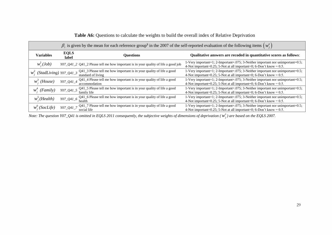
6 The weights are calculated according to the importance that each individual assigns to the S dimensions (see

Appendix A, Tab. A6). They vary between 0 (not important at all) to 1 (very important). Overall, the means of the

various dimensions are as follows: 0.75 for job, 0.84 for standard of living, 0.86 for accommodation, 0.92 for family

life, 0.95 for health and 0.82 for social life.

8

deprivation is lower than the median weighted sum of his reference group’s deprivations over all S

dimensions. This index is calculated as follows:

1

1_

0

A j A j

A j i Median

i A j A ji i Median

if s D s DOv s D

if s D s D

(6)

where A j A j

Median ii J

s D Median s D

.

Definition 7: Multidimensional index of subjective relative deprivation

The multidimensional index of subjective relative deprivation of individual i belonging to the j-th

reference group (R j

is D ) is the weighted sum of his deprivations over all S dimensions of deprivation

relative to the weighted sum of the indexes of relative deprivation over all S domains, assuming , 1j

i sRd

,s j . This index is calculated as follows:

,

1 1 1

S SR j s j s

i j i s ji s s

s D w Rd S w

(7)

Definition 8: Overall index of subjective relative deprivation

The overall index of subjective relative deprivation of individual i belonging to the jth reference group

( _ R j

iOv s D ) is equal to 1 if the weighted sum of his deprivations over all S dimensions of deprivation is

below the median weighted sum of his reference group’s deprivations over all S dimensions. This index is


1

1_

0

R j R j

R j i Median

i R j R ji i Median

if s D s DOv s D

if s D s D

(8)

where R j R j

Median ii J

s D Median s D

.

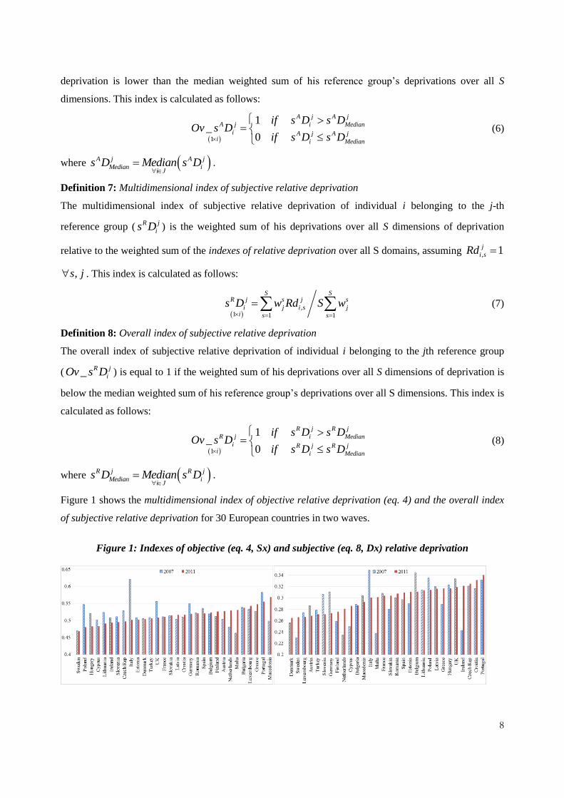
Figure 1 shows the multidimensional index of objective relative deprivation (eq. 4) and the overall index

of subjective relative deprivation for 30 European countries in two waves.

Figure 1: Indexes of objective (eq. 4, Sx) and subjective (eq. 8, Dx) relative deprivation

9

3.2 Descriptive Statistics and Reference Group Composition

The dataset is the European Quality of Life Survey, integrated data file 2003-2012 (EQLS, 2014). It is a

representative household survey of people aged eighteen and above. Carried out every four years, EQLS

examines a range of issues, such as employment, income, education, housing, family, health, work-life

balance, people's levels of happiness, life satisfaction, and perceived quality of society. In view of the

prospective European enlargements the geographical coverage of the survey has expanded over time from

28 countries in 2003 to 34 countries in 2011-12.

We selected from this survey, 30 countries for which we have data for the last two waves (2007 and

2011-12). To avoid having redundant information in the proposed indicators, we have combined some

items that were closely related (highly correlated).

Following the standard of empirical literature (e.g. Ferrer-i-Carbonell, 2005) the reference group of each

individual is assumed to be exogenous.7 In particular, to analyze the relative concerns in the determinant

of happiness, we assume that individual’s reference group depends by individual exogenous qualities as

education attainment, age, nationality. 8 We have a surveyed population of N=52,687 individuals,

representative of C=30 national populations. These 52,687 individuals are divided into J=552 reference

groups on the basis of a set of F=4 observable exogenous characteristics: (i) two waves, (ii) four age

classes, (iii) three education grades for each of (iv) 30 countries.9

Each individual faces S=6 relevant dimensions of deprivations: (i) labor, (ii) standard of life, (iii)

accommodation, (iv) family life, (v) health and (vi)social life. Each dimension is measured by

5,8,8,3,3,5sK sub-indicators. Details on EQLS and definition of different types of deprivations are

given in Appendix 1

4. Empirical Analysis

The main aim of the empirical analysis is to investigate the importance of different types of inequalities

and deprivations on subjective happiness.

Following the abundant empirical literature on the determinants of happiness (e.g., Argyle, 1999;

Lyubomirsky, 2001; Praag et al., 2003; Ferrer-i-Carbonell, 2005), we assume that individual utility can be

proxied by a self-reported happiness measure (h) that is affected by a set of observable demographic,

geographical, economic and cultural factors at the individual and aggregate levels. The question about

7 Falk and Knell (2004) present a theoretical model in which the reference group is endogenous. 8 It implies that individuals believe that education disparities are beyond individual’s responsibility but strongly

influenced by the family background. 9 The potential 720 reference groups became 552 because, there are 138 reference groups including greater than 20

individuals that we exclude to increase reliability of reference group statistics (e.g. within inequality). This cutting

reduces of 1.6% the total sample size.

10

happiness is strategically placed at the end of the EQLS questionnaire to avoid any framing effects of a

particular event dominating responses to the happiness question. 10

The following relationship is assumed for each individual i:

, , , ,meanh f y y Ineq Depr X (9)

where:

y is real OECD equalized income per capita;

meany is the expected value of real OECD equalized income per capita of the j-th reference group or

the c-th country of individual residence;

Ineq includes three indexes of income inequality - i.e., the relative income gap between the i-th

individual belonging to the j-th reference group and the richest peer max max

j i jy y y ;11 the Gini

index between reference groups for individual i belonging to the c-th country (between

cGini ); the Gini

index within a reference group for individual i belonging to the j-th reference group (within

jGini );

Depr denotes four alternative indexes of deprivation, as defined above (i.e.,

,

j

i sRd ; _ A j

iOv s D ; _ R j

iOv s D );

iX is a vector of standard socioeconomic variables both at the micro level - i.e., gender (Male), Age,

educational attainment (Edu), number of children (Hsize), marital status (Marital), employment status

(Worker) - and macroeconomic level - i.e., country of residence (CountryD) and time dummies (Year).

4.1. Econometric Specifications and Hypotheses

The baseline specification (eq. 10) is quite standard in the literature (e.g., Ferrer-i-Carbonell, 2005). It is

used to estimate the influence of equalized individual income and income at the country level (mean

cy ; see

Table 1, model I.a) or of the reference group (mean

jy ; Table 1, model I.b) on subjective well-being.

Following Deaton (2008) and Stevenson and Wolfers (2008, 2013), we assume that the happiness–

income relationship is roughly linear-log. Based on the economic and psychological literature on

happiness, we include standard demographic and economic variables (i.e., gender, age class, level of

education, number of children, marital status, employment status, year of survey, country of residence).

Fixing the reference categories in the model specification as unemployed, Austrian, 18-34 years old and

with compulsory education, as observed in 2007, the first specification is as follows:

10 In the EQLS questionnaire, the query is: Q41: Taking all things together on a scale of 1–10, how happy would

you say you are? Here 1 means you are very unhappy and 10 means you are very happy. 11 This index ranges from zero to one, where zero indicates that the ith individual is the richest in his/her reference

group. We interpret this index as a proxy for distance between individual expectations and actual position. In this

sense, it can be viewed as an alternative measure of income inequality within the reference group.

11

2

_

;

;

r

_

o

i

i i

ii i

mean

ci

i i

i

mean

ij

i

c

Edu sec Edu ter

Hsize

Marital

Worker

CountryD

Male

Ln Age Ln AgeLn y

Ln yh

Ln y

Year

(10)

where 1,...,52687i ; 1,...,552j and iYear is a period (i.e., wave) dummy variable that is equal to one

for the 2011-12 wave and zero for the 2007 wave.12

The second specification (equation 11) is used to test the impact of income inequality on subjective well-

being under a social comparison approach. First, we check whether our dataset validates the predominant

result in the literature that an increase in overall income inequality decreases individual happiness (Table

1, model II.a). Second, following Ferrer-i-Carbonell and Ramos’s (2014) suggestion, we decompose

income inequality into between and within reference groups (model II.b).13 Third, we enrich the model

specification by adding the multidimensional concept of absolute and relative deprivation to better

explain differences in subjective happiness depending on proxies for deprivation other than monetary

income (II.c-f). In sum, we add to the baseline regression both indexes of income inequality and

alternative indexes of deprivation, as defined in section 3.1:

6

,1

max max

_or

_

overall

c

jbetweeni sc s

withini j A j

meani i iij

R jj i ji

Ginior

RdGiniorLn y Gini

h XOv s DLn yor

y y yOv s D

(11)

Table 1 shows the econometric results for a selected subset of alternative specifications based on

regressions 10 and 11.

12 Ferrer-i-Carbonell and Frijters (2004) show that including a time constant individual fixed effect can considerably

change the estimated coefficients. Therefore, we control for this potential source of omitted variable bias. 13 When the Gini index is decomposed, a residual term arises given that income subgroups overlap (Lambert and

Aronson, 1993).

12

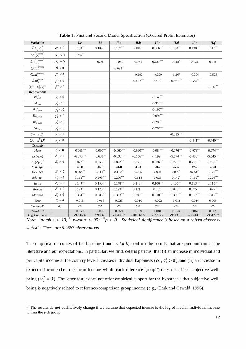
Table 1: First and Second Model Specification (Ordered Probit Estimator)

Variables I.a I.b II.a II.b II.c II.d II.e II.f

iLn y 1 0 0.189*** 0.189*** 0.187*** 0.184*** 0.066*** 0.104*** 0.130*** 0.113***

mean

cLn y 1

2 0 0.265***

mean

jLn y 2

2 0 -0.061 -0.050 0.081 0.237*** 0.161* 0.121 0.015

overall

cGini 1 0 -0.621**

between

cGini 2 0 -0.282 -0.220 -0.267 -0.294 -0.526

within

jGini 1

3 0 -0.527*** -0.713*** -0.661*** -0.584***

max max

j i jy y y 2

3 0 -0.143**

Deprivations

,

j

i JobRd 1

1 0 -0.146***

,

j

i StLivRd 2

1 0 -0.314***

,

j

i HouseRd 3

1 0 -0.195***

,

j

i FamilyRd 4

1 0 -0.094***

,

j

i HealthRd 5

1 0 -0.286***

,

j

i SocLRd 6

1 0 -0.286***

_ A j

iOv s D 2 0 -0.515***

_ R j

iOv s D 3 0 -0.441*** -0.440***

Controls

Male 1 0 -0.061*** -0.060*** -0.060*** -0.060*** -0.084*** -0.076*** -0.073*** -0.074***

Ln(Age) 2 0 -6.678*** -6.608*** -6.632*** -6.556*** -4.199*** -5.574*** -5.480*** -5.545***

Ln(Age)2 3 0 0.877*** 0.868*** 0.872*** 0.859*** 0.536*** 0.722*** 0.711*** 0.723***

Min. age 45.0 45.0 44.8 45.4 50.2 47.5 47.2 46.3

Edu_sec 4 0 0.094** 0.111** 0.110** 0.075 0.044 0.093* 0.090* 0.128***

Edu_ter 5 0 0.162*** 0.205*** 0.200*** 0.118 0.026 0.142* 0.152** 0.226***

Hsize 6 0 0.149*** 0.150*** 0.148*** 0.148*** 0.106*** 0.105*** 0.113*** 0.115***

Worker 7 0 0.123*** 0.123*** 0.123*** 0.121*** 0.031* 0.070*** 0.075*** 0.077***

Married 8 0 0.384*** 0.383*** 0.383*** 0.383*** 0.310*** 0.305*** 0.317*** 0.317***

Year 9 0 0.018 0.018 0.025 0.010 -0.022 -0.011 -0.014 0.000

CountryD c yes yes yes yes yes yes yes yes

Pseudo-R2 0.059 0.059 0.059 0.059 0.081 0.073 0.069 0.069

Log likelihood -99502.6 -99506.6 -99496.7 -100568.5 -97206.2 -99131.1 -98410.0 -98427.7

Note: *p-value < .10; ** p-value < .05; ***p < .01. Statistical significance is based on a robust cluster t-

statistic. There are 52,687 observations.

The empirical outcomes of the baseline (models I.a-b) confirm the results that are predominant in the

literature and our expectations. In particular, we find, ceteris paribus, that (i) an increase in individual and

per capita income at the country level increases individual happiness (1

1 2, 0 ), and (ii) an increase in

expected income (i.e., the mean income within each reference group14) does not affect subjective well-

being (2

2 0 ). The latter result does not offer empirical support for the hypothesis that subjective well-

being is negatively related to reference/comparison group income (e.g., Clark and Oswald, 1996).

14 The results do not qualitatively change if we assume that expected income is the log of median individual income

within the j-th group.

13

The effects of the standard control variables are as expected in the happiness literature: (i) females are

happier than males ( 1 0 ); (ii) a concave upward correlation exists between age and happiness such

that the least happy age is approximately 46 years old ( 2 0 ; 3 0 );15 (iii) larger-sized families (i.e.,

more people living together) are happier than smaller-sized families ( 6 0 ); (iv) people who are

married (or living with a partner) are happier than other individuals ( 7 0 ); (v) workers are happier

than unemployed people ( 8 0 ). Secondary- and tertiary-level education do not affect individual

happiness scores if we control for multidimensional deprivations, while they increase happiness scores in

more parsimonious model specifications ( 4 5, 0 in models I.a-b). We explain this lack of robustness

in the statistical significance of the coefficients by assuming that if multiple deprivation indexes are

included in the regression, they largely explain why a lack of education may affect happiness (e.g., worse

working conditions and health, unsatisfactory standards of living and social life).

Concerning the second specification (model II.a), our results corroborate the prevalent literature, which

supports the following proposition:

Proposition 1. An increase in overall inequality decreases individual happiness ( 1 0 ).

By contrast, the hypothesis of envy among peers has not been empirically validated, i.e.,

Proposition 2. An increase in mean income within a reference group does not affect subjective well-being

(2

2 0 ).

In the second step of the analysis, we decompose the Gini index to test whether individuals have different

tastes for inequality when judging peers than when examining society in general (models II.b-f). Ferrer-i-

Carbonell and Ramos (2014) assume that for reference groups defined in terms of educational attainment

and age, individuals believe that educational disparities are mostly caused by factors beyond the

individual’s responsibility, “...say, the family they are born into, but income differences of individuals

with similar education and age are mostly because of effort. We should then find a negative coefficient of

between inequality on happiness and a nil effect of within inequality” (p. 1019).

Our results reverse this expectation. We find a nil effect of between inequality on happiness and a

negative coefficient for within inequality. That is,

Proposition 3. People are not affected by between inequality ( 2 0 ).

Proposition 4. An increase of within inequality decreases individual happiness (1 2

3 3, 0 ).

Our interpretation is that in European countries, parents’ social class is not particularly relevant in

determining a child's educational achievement. As a consequence, if educational disparities mostly arise

15 According to a large literature of economists and behavioral scientists, an approximately U-shaped path of

happiness and well-being over the majority of the human lifespan has been documented by cross-sectional evidence

(e.g., Warr, 1992; Clark and Oswald, 1994; Frey and Stutzer, 2002; Ferrer-i-Carbonell, 2005; Blanchflower and

Oswald, 2008; Booth and van Ours, 2008; Baird et al. 2010; Cheng et al., 2015).

14

from differing abilities and effort levels, we should expect social acceptance of inequality between

reference groups. By contrast, income inequality among peers (in term of nationality, educational

attainment and age class) are perceived mostly as a consequence of factors beyond individuals’ control,

e.g., the underdevelopment of one’s geographic area of residence, differences in parental social networks,

a lack of job opportunities consistent with individual educational backgrounds, the absence of a

meritocracy, etc.

Our hypothesis follows Alesina et al.’s (2004) explanation that inequality should be less detrimental to

individual happiness if the society is perceived as mobile, as income inequality in that case would be

largely due to differences in individual effort and ability. We show that the authors’ proposition is valid

when individuals compare themselves with other members of their reference group, whereas inequality

does not reduce subjective well-being if is related to other social groups. In conclusion, we find that

Ferrer-i-Carbonell and Ramos’ (2014) hypothesis is inapplicable to European societies, while it may

apply to the educational system and labor market characteristics of the USA. This (untested) hypothesis

may suggest further research.

With respect to the indexes of deprivation (models II.c-f), we find that an increase in subjective,

objective, absolute or relative indexes of deprivation significantly decreases happiness ( 0 ).

The third set of specifications investigate whether different tastes for inequality, when judging peers and

when examining society in general, depend on an individual’s relative position at the national level

(Alesina et al., 2004) and within one’s reference group (Ferrer-i-Carbonell, 2005).

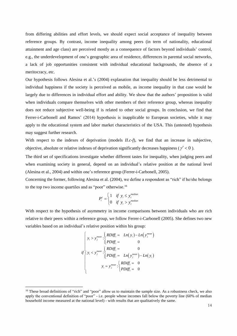
Concerning the former, following Alesina et al. (2004), we define a respondent as “rich” if he/she belongs

to the top two income quartiles and as “poor” otherwise.16

1

0

median

c i c

i median

i c

if y yP

if y y

With respect to the hypothesis of asymmetry in income comparisons between individuals who are rich

relative to their peers within a reference group, we follow Ferrer-i-Carbonell (2005). She defines two new

variables based on an individual’s relative position within his group:

:0

0:

0:

0

mean

i i jmean

i j

i

imean

i j mean

i j i

imean

i j

i

RDiff Ln y Ln yy y

PDiff

RDiffif y y

PDiff Ln y Ln y

RDiffy y

PDiff

16 These broad definitions of “rich” and “poor” allow us to maintain the sample size. As a robustness check, we also

apply the conventional definition of “poor” - i.e. people whose incomes fall below the poverty line (60% of median

household income measured at the national level) - with results that are qualitatively the same.

15

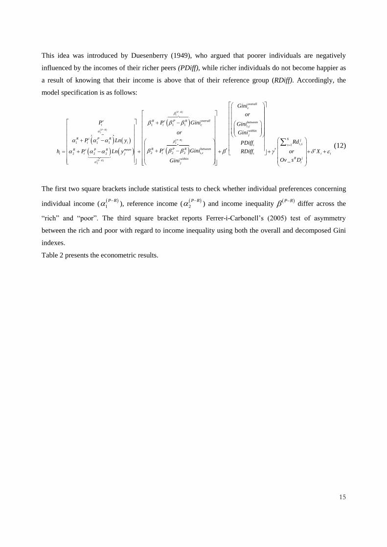
This idea was introduced by Duesenberry (1949), who argued that poorer individuals are negatively

influenced by the incomes of their richer peers (PDiff), while richer individuals do not become happier as

a result of knowing that their income is above that of their reference group (RDiff). Accordingly, the

model specification is as follows:

1

1

2

2

1 1 1

1 1 1

2 2 2 ,2 2 2

P R

P R

P R

P R

c R c P R overall

i i c

R c P R

i i

R c P R betweenR c P R meani i ci i j

within

j

P P Gini

or

P Ln y

P Ginih P Ln y

Gini

,

6

,1

_

overall

c

between

i c

within

j

j

i ssi

i i i

R j

i

Gini

or

Gini

Gini

RdPDiff

RDiff or X

Ov s D

(12)

The first two square brackets include statistical tests to check whether individual preferences concerning

individual income ( 1

P R

), reference income (

2

P R

) and income inequality

P R

differ across the

“rich” and “poor”. The third square bracket reports Ferrer-i-Carbonell’s (2005) test of asymmetry

between the rich and poor with regard to income inequality using both the overall and decomposed Gini

indexes.

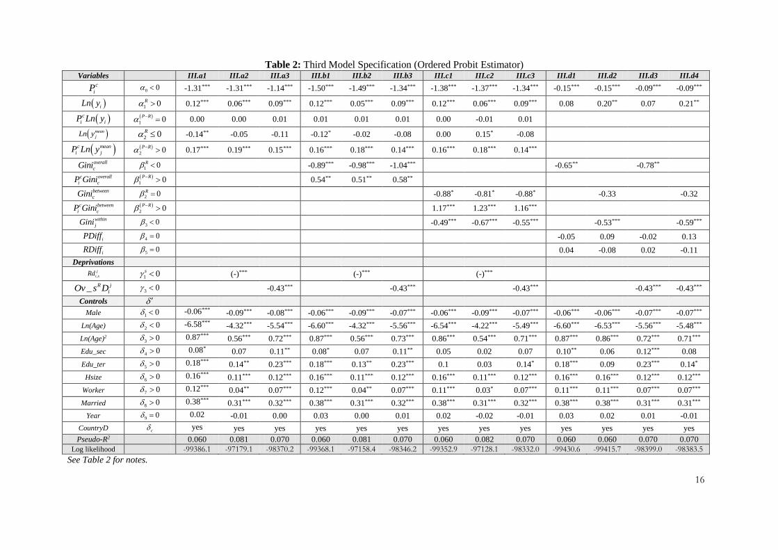
Table 2 presents the econometric results.

16

Table 2: Third Model Specification (Ordered Probit Estimator) Variables III.a1 III.a2 III.a3 III.b1 III.b2 III.b3 III.c1 III.c2 III.c3 III.d1 III.d2 III.d3 III.d4

c

iP 0 0 -1.31*** -1.31*** -1.14*** -1.50*** -1.49*** -1.34*** -1.38*** -1.37*** -1.34*** -0.15*** -0.15*** -0.09*** -0.09***

iLn y 1 0R 0.12*** 0.06*** 0.09*** 0.12*** 0.05*** 0.09*** 0.12*** 0.06*** 0.09*** 0.08 0.20** 0.07 0.21**

c

i iP Ln y 1 0

P R

0.00 0.00 0.01 0.01 0.01 0.01 0.00 -0.01 0.01

mean

jLn y 2 0R -0.14** -0.05 -0.11 -0.12* -0.02 -0.08 0.00 0.15* -0.08

c mean

i jP Ln y 2 0

P R

0.17*** 0.19*** 0.15*** 0.16*** 0.18*** 0.14*** 0.16*** 0.18*** 0.14***

overall

cGini 1 0R -0.89*** -0.98*** -1.04*** -0.65** -0.78**

c overall

i cP Gini 1 0

P R

0.54** 0.51** 0.58**

between

cGini 2 0R -0.88* -0.81* -0.88* -0.33 -0.32

c between

i cP Gini 2 0

P R

1.17*** 1.23*** 1.16***

within

jGini 3 0 -0.49*** -0.67*** -0.55*** -0.53*** -0.59***

iPDiff 4 0 -0.05 0.09 -0.02 0.13

iRDiff 5 0 0.04 -0.08 0.02 -0.11

Deprivations

,

j

i sRd 1 0s (-)*** (-)*** (-)***

_ R j

iOv s D 3 0 -0.43*** -0.43*** -0.43*** -0.43*** -0.43***

Controls

Male 1 0 -0.06*** -0.09*** -0.08*** -0.06*** -0.09*** -0.07*** -0.06*** -0.09*** -0.07*** -0.06*** -0.06*** -0.07*** -0.07***

Ln(Age) 2 0 -6.58*** -4.32*** -5.54*** -6.60*** -4.32*** -5.56*** -6.54*** -4.22*** -5.49*** -6.60*** -6.53*** -5.56*** -5.48***

Ln(Age)2 3 0 0.87*** 0.56*** 0.72*** 0.87*** 0.56*** 0.73*** 0.86*** 0.54*** 0.71*** 0.87*** 0.86*** 0.72*** 0.71***

Edu_sec 4 0 0.08* 0.07 0.11** 0.08* 0.07 0.11** 0.05 0.02 0.07 0.10** 0.06 0.12*** 0.08

Edu_ter 5 0 0.18*** 0.14** 0.23*** 0.18*** 0.13** 0.23*** 0.1 0.03 0.14* 0.18*** 0.09 0.23*** 0.14*

Hsize 6 0 0.16*** 0.11*** 0.12*** 0.16*** 0.11*** 0.12*** 0.16*** 0.11*** 0.12*** 0.16*** 0.16*** 0.12*** 0.12***

Worker 7 0 0.12*** 0.04** 0.07*** 0.12*** 0.04** 0.07*** 0.11*** 0.03* 0.07*** 0.11*** 0.11*** 0.07*** 0.07***

Married 8 0 0.38*** 0.31*** 0.32*** 0.38*** 0.31*** 0.32*** 0.38*** 0.31*** 0.32*** 0.38*** 0.38*** 0.31*** 0.31***

Year 9 0 0.02 -0.01 0.00 0.03 0.00 0.01 0.02 -0.02 -0.01 0.03 0.02 0.01 -0.01

CountryD c yes yes yes yes yes yes yes yes yes yes yes yes yes

Pseudo-R2 0.060 0.081 0.070 0.060 0.081 0.070 0.060 0.082 0.070 0.060 0.060 0.070 0.070

Log likelihood -99386.1 -97179.1 -98370.2 -99368.1 -97158.4 -98346.2 -99352.9 -97128.1 -98332.0 -99430.6 -99415.7 -98399.0 -98383.5

See Table 2 for notes.

17

The empirical results show, ceteris paribus, the following:

Proposition 5. The rich are happier than the poor ( 0 0 ).

Proposition 6. An increase in individual income increases the happiness of both the rich and the poor in

the same way ( 1 0 ; 1 0

P R

).

An increase in expected income reduces the happiness of the rich only if we do not control for income

inequality or deprivation (2 0R in models III.a1 and III.a2). Indeed, if any index of income distribution

and/or index of deprivation is included in the regression:

Proposition 7. The rich are unaffected by the average income of their peers (2 0R ).

This result corroborates previous results based on all individuals (see Table 1).

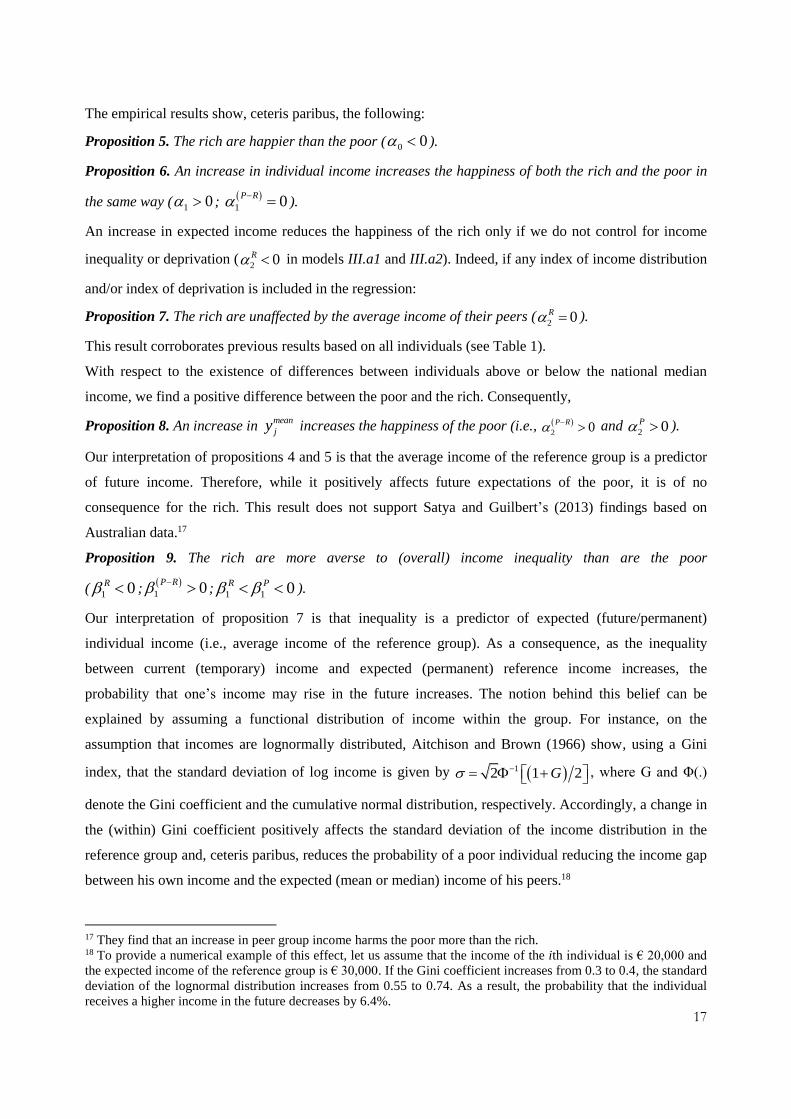
With respect to the existence of differences between individuals above or below the national median

income, we find a positive difference between the poor and the rich. Consequently,

Proposition 8. An increase in mean

jy increases the happiness of the poor (i.e., 2 0

P R

and

2 0P ).

Our interpretation of propositions 4 and 5 is that the average income of the reference group is a predictor

of future income. Therefore, while it positively affects future expectations of the poor, it is of no

consequence for the rich. This result does not support Satya and Guilbert’s (2013) findings based on

Australian data.17

Proposition 9. The rich are more averse to (overall) income inequality than are the poor

(1 0R ;

1 0

P R

;

1 1 0R P ).

Our interpretation of proposition 7 is that inequality is a predictor of expected (future/permanent)

individual income (i.e., average income of the reference group). As a consequence, as the inequality

between current (temporary) income and expected (permanent) reference income increases, the

probability that one’s income may rise in the future increases. The notion behind this belief can be

explained by assuming a functional distribution of income within the group. For instance, on the

assumption that incomes are lognormally distributed, Aitchison and Brown (1966) show, using a Gini

index, that the standard deviation of log income is given by 12 1 2G , where G and Φ(.)

denote the Gini coefficient and the cumulative normal distribution, respectively. Accordingly, a change in

the (within) Gini coefficient positively affects the standard deviation of the income distribution in the

reference group and, ceteris paribus, reduces the probability of a poor individual reducing the income gap

between his own income and the expected (mean or median) income of his peers.18

17 They find that an increase in peer group income harms the poor more than the rich. 18 To provide a numerical example of this effect, let us assume that the income of the ith individual is € 20,000 and

the expected income of the reference group is € 30,000. If the Gini coefficient increases from 0.3 to 0.4, the standard

deviation of the lognormal distribution increases from 0.55 to 0.74. As a result, the probability that the individual

receives a higher income in the future decreases by 6.4%.

18

Proposition 10. The rich are not averse to income inequality between groups (with the exception of III.c2).

By contrast, an increase in the between group Gini index (often) increases the happiness of the poor

(2 0R ;

2 0

P R

;

2 20R P ).

Proposition 11. An increase in the income gap between individuals (rich and poor) and the mean income

of the reference group does not increase happiness ( 4 0 ; 5 0 ).

While this result confirms Ferrer-i-Carbonell’s (2005) findings for the rich, it does not corroborate the

expected negative influence of the income of richer peers on poor individuals. As a result, we derive

Lemma 1. There is no evidence, at the European level, of asymmetry in preferences for equality between

the rich and poor using both overall and decomposed Gini indexes.

In conclusion, we test the robustness of previous findings by replicating the empirical analysis using: (1)

McBride’s (2001) approach to defining reference groups with respect to age classes, where all individuals

five years younger and five years older than the target individual are included in the individual’s

reference group; (2) reducing from 20 to 10 the minimal threshold for excluding reference groups with

insufficient numbers of individuals to suitably estimate the within Gini index; (3) doubling the number of

reference groups by also defining reference groups in terms of gender. These robustness tests largely

confirm the main propositions reported above.

5. Conclusions

This paper aims to contribute to the economics literature on inequality and happiness in two ways: (i) by

decomposing the overall income inequality effect on happiness into a within group inequality effect and a

between group inequality effect at the country level; (ii) by extending the concept of social comparison to

the domain of income, i.e., by considering different dimensions of subjective (i.e., self-declared) and

relative “objective” deprivation.

According to Ferrer-i-Carbonell and Ramos (2014), there is robust evidence that an individual’s position

in the income distribution of his reference group affects his well-being. This hypothesis derives from the

third hypothesis of Festinger’s (1954) theory of social comparison processes, which assumes that the

tendency to compare oneself with some other specific person decreases as the difference between the

other’s characteristics and abilities and one's own characteristics and abilities increases. Ferrer-i-

Carbonell and Ramos (2014) hypothesize that if individuals have different preferences regarding those

who they perceive as equals (i.e., within inequality) and those who they perceive as non-equals (between

inequality), the income distribution of each group will also have a different impact on happiness. They

expect a negative effect of between inequality on happiness and a non-statistically significant effect of

within inequality on happiness. Ferrer-i-Carbonell and Ramos (2014) don’t empirically test these

predictions but, according to the authors, they “would also be consistent (and even reconcile) the two

19

findings in the happiness literature: a negative effect of overall inequality and a positive effect of being at

the top of the income distribution of own reference group (p. 1019)”.

In this research, we find empirical support for their hypothesis of differing effects of within and between

inequality on happiness, but the signs of these effects vary. In particular, within reference group

inequality negatively affects happiness, and between group inequality has no statistically significant effect

on subjective well-being.

We propose two not necessarily exclusive interpretations of these findings: (i) happiness is partly

determined by comparisons with others with respect to income distribution and relative deprivations

among peers. These factors better explains the variability of individual happiness than overall or between

inequality among groups; (ii) as the mean income in the reference group may indicate expected future

income (see Hirschman and Rothschild 1973), mutatis mutandis, income distribution could indirectly

indicate the likelihood that one’s own future income will not be lower than the expected future income.

Given that greater inequality increases the skewness of the income distribution, the probability of earning

an income below the expected income increases, and consequently, individual happiness decreases,

ceteris paribus.19

Finally, we obtain robust evidence that a low absolute individual income has a smaller marginal effect on

individual happiness than the other dimensions of deprivation (job conditions, standard of living, housing

conditions, family, health and social life). The policy implication may be that providing access to good

health care and other forms of social assistance, reducing the precariousness of labor market conditions

(thereby improving opportunities to support a family), improving living standards and enhancing social

inclusion will achieve the maximum gain in societal well-being, increasing both net individual income

and reference group income.

19 An alternative interpretation is that the index of inequality could be considered a measure of the numerator of a

coefficient of variation (i.e., the ratio of the standard deviation to the mean) such that as inequality increases, the

dispersion around the mean increases, and increased risk aversion reduces utility.

20

References

Aitchison, J., Brown, J.A.C. 1963. The Lognormal Distribution. Cambridge University Press, New York.

Alesina, A., Di Tella, R., MacCulloch, R. (2004). Inequality and happiness: Are Europeans and

Americans different? Journal of Public Economics, 88, 2009–2042.

Alesina, A., Glaeser, E., Sacerdote, B., (2001). Why doesn’t the United States have a European-style

welfare state? Brookings papers on Economic Activity, 2, 187-277.

Amendola A., Dell’Anno R. (2015). Social Exclusion and economic growth: an empirical investigation in

European economies. Review of Income and Wealth., 61(2), 274-301.

Argyle, M. (1999). Causes and correlates of happiness. In Kahneman, Daniel (Ed); Diener, Ed (Ed);

Schwarz, Norbert (Ed), (1999). Well-being: The foundations of hedonic psychology, (pp. 353-373).

New York, NY, US: Russell Sage Foundation.

Baird, B., Lucas, R.E., Donovan, M. B. (2010). Life satisfaction across the life span: Findings from two

nationally representative panel studies. Social Indicators Research, 99, 183-203.

Bellani L. (2013). Multidimensional indices of deprivation: the introduction of reference groups weights.

The Journal of Economic Inequality, 11(4): 495-515.

Bjørnskov, C., Dreher, A., Fischer, J. A.V., Schnellenbach, J., Gehring, K., (2013). Inequality and

happiness: When perceived social mobility and economic reality do not match, Journal of

Economic Behavior & Organization, 91(C), 75-92.

Blanchflower, D. G., Oswald, A. J., (2011). International Happiness, NBER Working Papers 16668,

National Bureau of Economic Research, Inc.

Blanchflower, D. G., Oswald, A.J. (2008). Is well-being U-shaped over the life cycle?, Social Science

and Medicine 66, 1733–1749.

Booth, A. L., van Ours, J. C. (2008). Job satisfaction and family happiness: the part‐time work puzzle.

The Economic Journal, 118(526), F77-F99.

Bossert, W., D’Ambrosio, C., Peragine, V. (2007). Deprivation and Social Exclusion. Economica,

74(296), 777-803

Burchardt, T., Le Grand, J., Piachaud, D. (1999). Social exclusion in Britain 1991-1995, Social Policy

and Administration, 33,227-244.

Cheng, T. C., Powdthavee, N., Oswald, A. J, (2015). Longitudinal Evidence for a Midlife Nadir in

Human Wellbeing: Results from Four Data Sets. The Economic Journal DOI: 10.1111/ecoj.12256.

Clark, A. E., Oswald, A. J. (1994). Unhappiness and unemployment. Economic Journal, 104, 648-659.

Clark, A. E., Oswald, A. J. (1996). Satisfaction and comparison income. Journal of Public Economics,

61, 359-381.

Clark, A. E., Frijters, P., Shields, M. A. (2008). Relative Income, Happiness, and Utility: An Explanation

for the Easterlin Paradox and Other Puzzles. Journal of Economic Literature, 46(1), 95-144.

Corcoran, K., Crusius, J., Mussweiler, T. (2011). Social Comparison: Motives, Standards, and

Mechanisms. In D. Chadee (Ed.) Theories in social psychology. Oxford, UK: Wiley-Blackwell.

pp.119-139.

Chakravarty, S. R., D’Ambrosio C. (2006). The Measurement of Social Exclusion. Review of Income and

Wealth, 52, 377-398.

Deaton, A. (2008). Income, Health, and Well-Being around the World: Evidence from the Gallup World

Poll. Journal of Economic Perspectives, 22(2), 53-72.

Diener, E., Ng, W., Harter, J., Arora, R.(2010).Wealth and happiness across the world: Material

prosperity predicts life evaluation, whereas psychosocial prosperity predicts positive feeling.

Journal of Personality and Social Psychology, 99, 52–61.

21

Diener, E., Sandvik, E. Seidlitz, L., Diener, M. (1993). The relationship between income and subjective

well-being: Relative or absolute? Social Indicators Research, 28, 195-223.

Duesenberry, J. S. (1949). Income, Saving, and the Theory of Consumer Behavior, Harvard University

Press.

Easterlin, R. (2001), Income and Happiness: Towards a Unified Theory. The Economic Journal, 111,

465-484.

Easterlin, R. (1974). Does Economic Growth Improve the Human Lot? In Paul A. David and Melvin W.

Reder, eds., Nations and Households in Economic Growth: Essays in Honor of Moses Abramovitz,

New York: Academic Press, Inc.

Easterlin, R. (1995) Will raising the incomes of all increase the happiness of all. Journal of Economic

Behaviour and Organization, 27, 35-47.

EQLS (2014). European Foundation for the Improvement of Living and Working Conditions, European

Quality of Life Survey Integrated Data File, 2003-2012 [computer file]. 2nd Edition. Colchester,

Essex: UK Data Archive [distributor], January 2014. SN: 7348 , http://dx.doi.org/10.5255/UKDA-

SN-7348-2.

Falk, A., Knell, M. (2004). Choosing the Joneses: On the Endogeneity of Reference Groups,

Scandinavian Journal of Economics, 106, 417-35.

Ferrer-i-Carbonell, A., Ramos, X. (2014). Inequality and Happiness. Journal of Economic Surveys, 28(

5), 1016–1027.

Ferrer-i-Carbonell A., Ramos, X., (2010). Inequality Aversion and Risk Attitudes," SOEP papers on

Multidisciplinary Panel Data Research 271, DIW Berlin, The German Socio-Economic Panel

(SOEP).

Ferrer-i-Carbonell, A. (2005). Income and well-being: an empirical analysis of the comparison income

effect. Journal of Public Economics, 89, 997-1019.

Ferrer-i-Carbonell, A., Frijters, P. (2004). How important is methodology for the estimates of the

determinants of happiness? The Economic Journal, 114, 641-659.

Festinger, L. (1954). A theory of social comparison processes. Human Relations, 7(2), 117-140.

FitzRoy, F., Nolan, M., Steinhardt, M., Ulph, D. (2014). Testing the Tunnel Effect: Comparison, Age and

Happiness in UK and German Panels, IZA Journal of European Labor Studies, 3, 1-24.

Frey, B.S., Stutzer A. (2000), Happiness, Economy and Institutions, Economic Journal, 110, 918-938.

Frey, B.S., Stutzer, A. (2002). Happiness and Economics: How the Economy and Institutions Affect

Well-Being, Princeton: Princeton University Press.

Frey, B. S., and Stutzer, A. (2004). Economic Consequences of Mispredicting Utility. Journal of

Happiness Studies, 15(4): 937-956.

Frey, B., Schmidt, S., Torgler, B. (2008) Relative income position, inequality and performance: An

empirical panel analysis. In Andersson, P, Ayton, P, & Schmidt, C (Eds.) Myths and Facts About

Football - The Economics and Psychology of the World's Greatest Sport. Cambridge Scholars

Publishing, United Kingdom, Newcastle upon Tyne, pp. 349-369

Groot, W., van den Brink, H. M. (1999). Overpayment and Earnings Satisfaction: An Application of an

Ordered Response Tobit Model. Applied Economics Letters, 6, 235-238.

Gruber, J., Mullainathan, S. (2005). Do cigarette taxes make smokers happier?. The B.E. Journal of

Economic Analysis & Policy, 1(5), article 4.

Hirschman, A. O., Rothschild, M. (1973). The Changing Tolerance for Income Inequality in the Course

of Economic Development; with a Mathematical Appendix. The Quarterly Journal of Economics,

87(4), 544-566.

http://dx.doi.org/10.5255/UKDA-SN-7348-2

http://dx.doi.org/10.5255/UKDA-SN-7348-2

22

Johns, H., Ormerod, P. (2008). Happiness, Economics and Public Policy. The Institute of Economic

Affairs, London, UK.

Kahneman, D., (1999). Objective Happiness, in Daniel Kahneman, Ed Diener and Norbert Schwarz eds.,

Well-Being: The Foundations of Hedonic Psychology, chapter 1. Russell Sage Foundation, New

York.

Kahneman, D., Deaton, A., (2010). High income improves evaluation of life but not emotional well-

being, Proceedings of the National Academy of Sciences 107, 38: 16489-16493.

Kahneman, D., Diener E., Schwarz N. (eds.), (1999) Well-Being: The Foundations of Hedonic

Psychology, Russell Sage Foundation, New York.

Kahneman, D., Krueger A. B. (2006). Developments in the Measurement of Subjective Well-Being.

Journal of Economic Perspectives, 20(1): 3-24.

Kimball, M. and Willis, R. (2006). “Utility and Happiness”. University of Michigan, Department of

Economics, Working Paper, March 3.

Lambert, P. J, Aronson J. R. (1993). Inequality Decomposition Analysis and the Gini Coefficient

Revisited. The Economic Journal, 103(420),1221-1227.

Layard, R. (2005). Rethinking public economics: the implications of rivalry and habit, in L. Bruni and

P.L. Porta, (eds.), Economics and Happiness: Reality and Paradoxes, pp. 147–69, Oxford: Oxford

University Press.

Layard, R. (2006). Happiness and public policy: a challenge to the profession. The Economic Journal,

116(March), C24–C33.

Luttmer, E. F. P. (2005). Neighbors As Negatives: Relative Earnings and Well-Being, Quarterly Journal

of Economics. 120: 963-1002.

Lyubomirsky, S. (2001). Why Are Some People Happier Than Others? The Role of Cognitive and

Motivational Processes in Well-Being. American Psychologist. 56: 239-249.

McBride, M. (2001). Relative-Income Effects on Subjective Well-Being in the Cross-Section, Journal of

Economic Behavior and Organization. 45: 251-278.

Praag, B.M.S., Frijters, P., Ferrer-i-Carbonell, A., (2003). The anatomy of subjective well-being, Journal

of Economic Behavior and Organization, 51, 29-49.

Satya P., Guilbert D. (2013). Income–happiness paradox in Australia: Testing the theories of adaptation

and social comparison, Economic Modelling, 30, 900-910.

Stevenson Betsey and Justin Wolfers (2008). Economic Growth and Subjective Well-Being: Reassessing

the Easterlin Paradox. Brookings Papers on Economic Activity 39(1): 1-102.

Stevenson, Betsey, and Justin Wolfers. 2013. Subjective Well-Being and Income: Is There Any Evidence

of Satiation?" American Economic Review, 103(3), 598-604.

Stutzer, A. (2004). The Role of Income Aspirations in Individual Happiness, Journal of Economic

Behavior and Organization. 54: 89-109

Tsakloglou, P., Papadopoulos, F., (2002), Identifying Population Groups at High Risk of Social

Exclusion: Evidence from the ECHP, in: R.J.A. Muffels, P. Tsakloglou and D.G. Mayes (eds.),

Social Exclusion in European Welfare States, Edward Elgar, Cheltenham, Chapter 6.

Thurow, L. (1971). The Income Distribution as a Pure Public Good”, Quarterly Journal of Economics, 83,

327-336.

Tsou, M. W., Liu, J. T. (2001). Happiness and Domain Satisfaction in Taiwan, Journal of Happiness

Studies. 2: 269-88.

Veenhoven R., (1991). Is happiness relative? Social Indicators Research, 24, 1-34.

23

Veenhoven R., Hagerty M., (2006). Rising happiness in nations 1946-2004. Social Indicators Research,

79, 421-436.

Warr, P. (1992). Age and occupational well-being. Psychology and Aging, 7, 37-45.

Watson, R., Storey, D., Wynarczyk, P., Keasey K., Short H. (1996). The Relationship Between Job

Satisfaction and Managerial Remuneration in Small and Medium-Sized Enterprises: An Empirical

Test of ‘Comparison Income’ and ‘Equity Theory’ Hypotheses, Applied Economics. 28: 567-76.

24

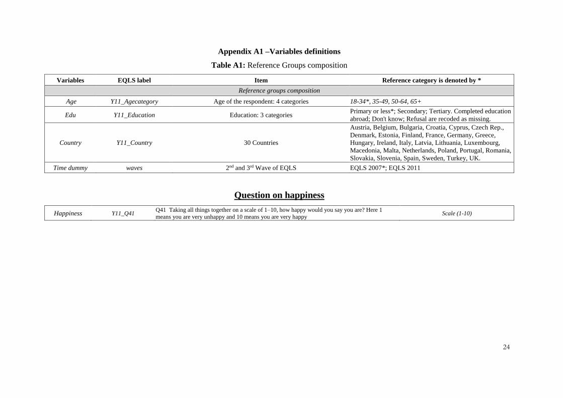
Appendix A1 –Variables definitions

Table A1: Reference Groups composition

Variables EQLS label Item Reference category is denoted by *

Reference groups composition

Age Y11_Agecategory Age of the respondent: 4 categories 18-34*, 35-49, 50-64, 65+

Edu Y11_Education Education: 3 categories Primary or less*; Secondary; Tertiary. Completed education

abroad; Don't know; Refusal are recoded as missing.

Country Y11_Country 30 Countries

Austria, Belgium, Bulgaria, Croatia, Cyprus, Czech Rep.,

Denmark, Estonia, Finland, France, Germany, Greece,

Hungary, Ireland, Italy, Latvia, Lithuania, Luxembourg,

Macedonia, Malta, Netherlands, Poland, Portugal, Romania,

Slovakia, Slovenia, Spain, Sweden, Turkey, UK.

Time dummy waves 2nd and 3rd Wave of EQLS EQLS 2007*; EQLS 2011

Question on happiness

Happiness Y11_Q41 Q41 Taking all things together on a scale of 1–10, how happy would you say you are? Here 1

means you are very unhappy and 10 means you are very happy Scale (1-10)

25

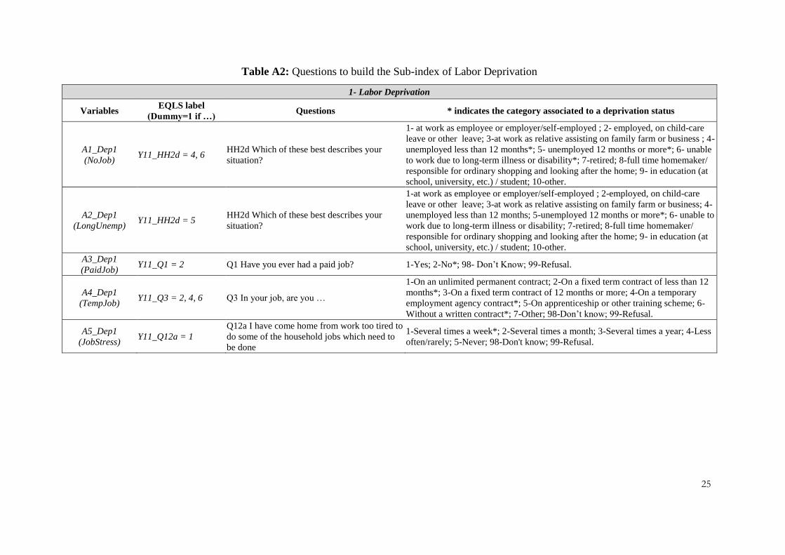
Table A2: Questions to build the Sub-index of Labor Deprivation

1- Labor Deprivation

Variables EQLS label

(Dummy=1 if …) Questions * indicates the category associated to a deprivation status

A1_Dep1

(NoJob) Y11_HH2d = 4, 6

HH2d Which of these best describes your

situation?

1- at work as employee or employer/self-employed ; 2- employed, on child-care

leave or other leave; 3-at work as relative assisting on family farm or business ; 4-

unemployed less than 12 months*; 5- unemployed 12 months or more*; 6- unable

to work due to long-term illness or disability*; 7-retired; 8-full time homemaker/

responsible for ordinary shopping and looking after the home; 9- in education (at

school, university, etc.) / student; 10-other.

A2_Dep1

(LongUnemp) Y11_HH2d = 5

HH2d Which of these best describes your

situation?

1-at work as employee or employer/self-employed ; 2-employed, on child-care

leave or other leave; 3-at work as relative assisting on family farm or business; 4-

unemployed less than 12 months; 5-unemployed 12 months or more*; 6- unable to

work due to long-term illness or disability; 7-retired; 8-full time homemaker/

responsible for ordinary shopping and looking after the home; 9- in education (at

school, university, etc.) / student; 10-other.

A3_Dep1

(PaidJob) Y11_Q1 = 2 Q1 Have you ever had a paid job? 1-Yes; 2-No*; 98- Don’t Know; 99-Refusal.

A4_Dep1

(TempJob) Y11_Q3 = 2, 4, 6 Q3 In your job, are you …

1-On an unlimited permanent contract; 2-On a fixed term contract of less than 12

months*; 3-On a fixed term contract of 12 months or more; 4-On a temporary

employment agency contract*; 5-On apprenticeship or other training scheme; 6-

Without a written contract*; 7-Other; 98-Don’t know; 99-Refusal.

A5_Dep1

(JobStress) Y11_Q12a = 1

Q12a I have come home from work too tired to

do some of the household jobs which need to

be done

1-Several times a week*; 2-Several times a month; 3-Several times a year; 4-Less

often/rarely; 5-Never; 98-Don't know; 99-Refusal.

26

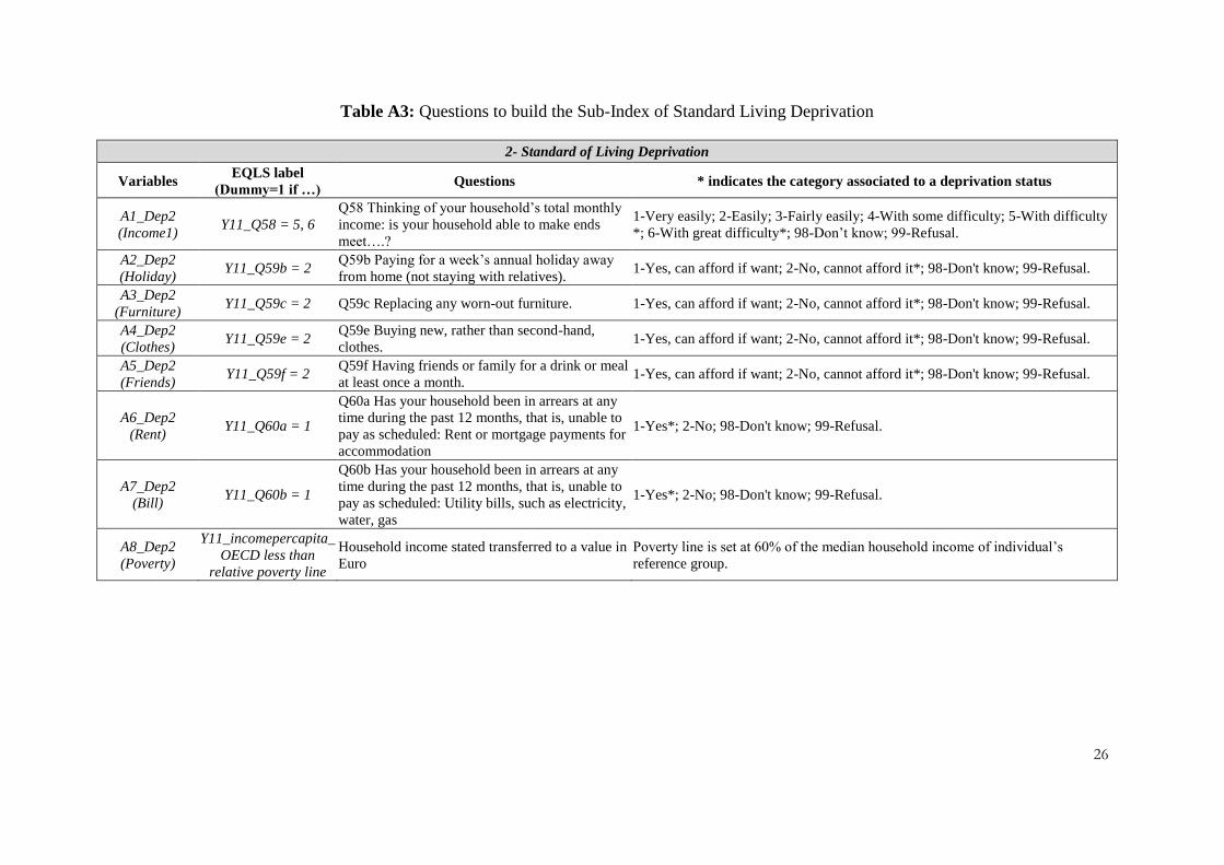
Table A3: Questions to build the Sub-Index of Standard Living Deprivation

2- Standard of Living Deprivation



A1_Dep2

(Income1) Y11_Q58 = 5, 6

Q58 Thinking of your household’s total monthly

income: is your household able to make ends

meet….?

1-Very easily; 2-Easily; 3-Fairly easily; 4-With some difficulty; 5-With difficulty

*; 6-With great difficulty*; 98-Don’t know; 99-Refusal.

A2_Dep2

(Holiday) Y11_Q59b = 2

Q59b Paying for a week’s annual holiday away

from home (not staying with relatives). 1-Yes, can afford if want; 2-No, cannot afford it*; 98-Don't know; 99-Refusal.

A3_Dep2

(Furniture) Y11_Q59c = 2 Q59c Replacing any worn-out furniture. 1-Yes, can afford if want; 2-No, cannot afford it*; 98-Don't know; 99-Refusal.

A4_Dep2

(Clothes) Y11_Q59e = 2

Q59e Buying new, rather than second-hand,

clothes. 1-Yes, can afford if want; 2-No, cannot afford it*; 98-Don't know; 99-Refusal.

A5_Dep2

(Friends) Y11_Q59f = 2

Q59f Having friends or family for a drink or meal

at least once a month. 1-Yes, can afford if want; 2-No, cannot afford it*; 98-Don't know; 99-Refusal.

A6_Dep2

(Rent) Y11_Q60a = 1

Q60a Has your household been in arrears at any

time during the past 12 months, that is, unable to

pay as scheduled: Rent or mortgage payments for

accommodation

1-Yes*; 2-No; 98-Don't know; 99-Refusal.

A7_Dep2

(Bill) Y11_Q60b = 1

Q60b Has your household been in arrears at any

time during the past 12 months, that is, unable to

pay as scheduled: Utility bills, such as electricity,

water, gas

1-Yes*; 2-No; 98-Don't know; 99-Refusal.

A8_Dep2

(Poverty)

Y11_incomepercapita_

OECD less than

relative poverty line

Household income stated transferred to a value in

Euro

Poverty line is set at 60% of the median household income of individual’s

reference group.

27

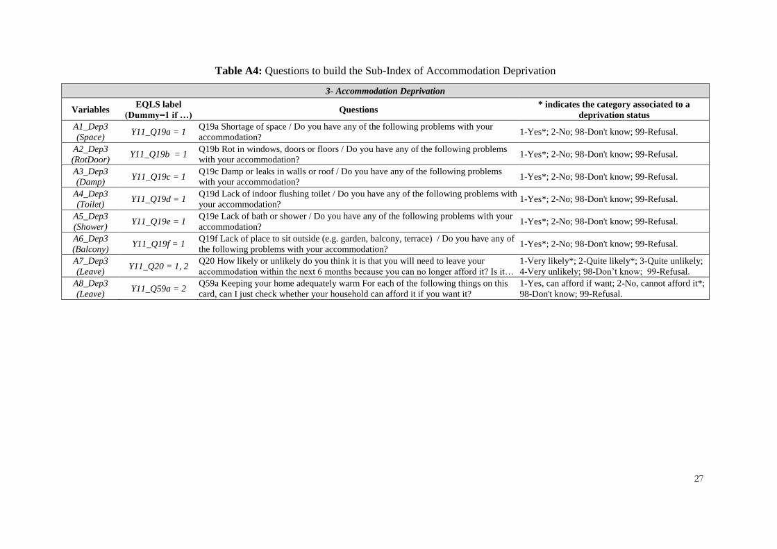
Table A4: Questions to build the Sub-Index of Accommodation Deprivation

3- Accommodation Deprivation


(Dummy=1 if …) Questions

* indicates the category associated to a

deprivation status

A1_Dep3

(Space) Y11_Q19a = 1

Q19a Shortage of space / Do you have any of the following problems with your

accommodation? 1-Yes*; 2-No; 98-Don't know; 99-Refusal.

A2_Dep3

(RotDoor) Y11_Q19b = 1

Q19b Rot in windows, doors or floors / Do you have any of the following problems

with your accommodation? 1-Yes*; 2-No; 98-Don't know; 99-Refusal.

A3_Dep3

(Damp) Y11_Q19c = 1

Q19c Damp or leaks in walls or roof / Do you have any of the following problems

with your accommodation? 1-Yes*; 2-No; 98-Don't know; 99-Refusal.

A4_Dep3

(Toilet) Y11_Q19d = 1

Q19d Lack of indoor flushing toilet / Do you have any of the following problems with

your accommodation? 1-Yes*; 2-No; 98-Don't know; 99-Refusal.

A5_Dep3

(Shower) Y11_Q19e = 1

Q19e Lack of bath or shower / Do you have any of the following problems with your

accommodation? 1-Yes*; 2-No; 98-Don't know; 99-Refusal.

A6_Dep3

(Balcony) Y11_Q19f = 1

Q19f Lack of place to sit outside (e.g. garden, balcony, terrace) / Do you have any of

the following problems with your accommodation? 1-Yes*; 2-No; 98-Don't know; 99-Refusal.

A7_Dep3

(Leave) Y11_Q20 = 1, 2

Q20 How likely or unlikely do you think it is that you will need to leave your

accommodation within the next 6 months because you can no longer afford it? Is it…

1-Very likely*; 2-Quite likely*; 3-Quite unlikely;

4-Very unlikely; 98-Don’t know; 99-Refusal.

A8_Dep3

(Leave) Y11_Q59a = 2

Q59a Keeping your home adequately warm For each of the following things on this

card, can I just check whether your household can afford it if you want it?

1-Yes, can afford if want; 2-No, cannot afford it*;

98-Don't know; 99-Refusal.

28

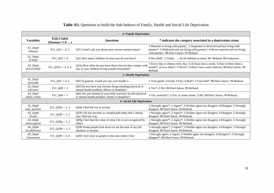
Table A5: Questions to build the Sub-Indexes of Family, Health and Social Life Deprivation

4- Family Deprivation



A1_Dep4

(Status) Y11_Q31 = 2, 3 Q31 Could I ask you about your current marital status?

1-Married or living with partner; 2-Separated or divorced and not living with

partner*; 3-Widowed and not living with partner*; 4-Never married and not living

with partner; 98-Don’t know; 99-Refusal.

A2_Dep4

(Child) Y11_Q32 = 0 Q32 How many children of your own do you have? 0-No child*; 1-Child; …; 10-10 children or more; 99- Refusal; 98-Unknown.

A3_Dep4

(FaceChild) Y11_Q33a = 3, 4, 5

Q33a How often do you have direct face-to-face contact with

any of your children living outside household?

1-Every day or almost every day; 2-At least once a week; 3-One to three times a

month*; 4-Less often*; 5-Never*; 6-Don’t have such relatives; 98-Don't know; 99-

Refusal.

5- Health Deprivation

A1_Dep5

(overall) Y11_Q42 = 4, 5 Q42 In general, would you say your health is … 1-Very good; 2-Good; 3-Fair; 4-Bad*; 5-Very bad*; 98-Don’t know: 99-Refusal.

A2_Dep5

(chronic) Y11_Q43 = 1

Q43 Do you have any chronic (long-standing) physical or

mental health problem, illness or disability? 1-Yes*; 2-No; 98-Don't know; 99-Refusal.

A3_Dep5

(daily_limit) Y11_Q44 = 1

Q44 Are you limited in your daily activities by this physical

or mental health problem, illness or disability? 1-Yes, severely*; 2-Yes, to some extent; 3-No; 98-Don’t know; 99-Refusal.

6- Social Life Deprivation

A1_Dep6

(out_society) Y11_Q29e = 1, 2 Q29e I feel left out of society

1-Strongly agree*; 2-Agree*; 3-Neither agree nor disagree; 4-Disagree; 5-Strongly

disagree; 98-Don't know; 99-Refusal.

A2_Dep6

(Lost) Y11_Q29f = 1, 2

Q29f Life has become so complicated today that I almost

can’t find my way



A3_Dep6

(unrecogniz) Y11_Q29g = 1, 2

Q29g I feel that the value of what I do is not recognized by

others



A4_Dep6

(LookDown) Y11_Q29h = 1, 2

Q29h Some people look down on me because of my job

situation or income



A5_Dep6

(closeness) Y11_Q29i = 5, 6 Q29i I feel close to people in the area where I live

1-Strongly agree; 2-Agree; 3-Neither agree nor disagree; 4-Disagree*; 5-Strongly

disagree*; 98-Don't know; 99-Refusal.

29

Table A6: Questions to calculate the weights to build the overall index of Relative Deprivation

Note: The question Y07_Q41 is omitted in EQLS 2011 consequently, the subjective weights of dimensions of deprivation (s

jw ) are based on the EQLS 2007.

i is given by the mean for each reference group$ in the 2007 of the self-reported evaluation of the following items s

jw

Variables EQLS

label Questions Qualitative answers are recoded in quantitative scores as follows:

1

jw (Job) Y07_Q41_2 Q41_2 Please tell me how important is in your quality of life a good job 1-Very important=1; 2-Important=.075; 3-Neither important nor unimportant=0.5;

4-Not important=0.25; 5-Not at all important=0; 6-Don’t know = 0.5.

2

jw (StadLiving) Y07_Q41_3 Q41_3 Please tell me how important is in your quality of life a good

standard of living

1-Very important=1; 2-Important=.075; 3-Neither important nor unimportant=0.5;


3

jw (House) Y07_Q41_4 Q41_4 Please tell me how important is in your quality of life a good

accommodation



4

jw (Family) Y07_Q41_5 Q41_5 Please tell me how important is in your quality of life a good

family life



5

jw (Health) Y07_Q41_6 Q41_6 Please tell me how important is in your quality of life a good

health



6

jw (SocLife) Y07_Q41_7 Q41_7 Please tell me how important is in your quality of life a good

social life



30

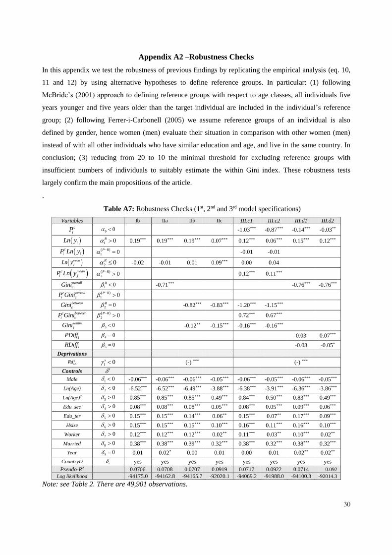
Appendix A2 –Robustness Checks

In this appendix we test the robustness of previous findings by replicating the empirical analysis (eq. 10,

11 and 12) by using alternative hypotheses to define reference groups. In particular: (1) following

McBride’s (2001) approach to defining reference groups with respect to age classes, all individuals five

years younger and five years older than the target individual are included in the individual’s reference

group; (2) following Ferrer-i-Carbonell (2005) we assume reference groups of an individual is also

defined by gender, hence women (men) evaluate their situation in comparison with other women (men)

instead of with all other individuals who have similar education and age, and live in the same country. In

conclusion; (3) reducing from 20 to 10 the minimal threshold for excluding reference groups with

insufficient numbers of individuals to suitably estimate the within Gini index. These robustness tests

largely confirm the main propositions of the article.

.

Table A7: Robustness Checks (1st, 2nd and 3rd model specifications)

Variables Ib IIa IIb IIc III.c1 III.c2 III.d1 III.d2 c

iP 0 0 -1.03*** -0.87*** -0.14*** -0.03**

iLn y 1 0R 0.19*** 0.19*** 0.19*** 0.07*** 0.12*** 0.06*** 0.15*** 0.12***

c

i iP Ln y 1 0

P R

-0.01 -0.01

mean

jLn y 2 0R -0.02 -0.01 0.01 0.09*** 0.00 0.04

c mean

i jP Ln y 2 0

P R

0.12*** 0.11***

overall

cGini 1 0R -0.71*** -0.76*** -0.76***

c overall

i cP Gini 1 0

P R

between

cGini 2 0R -0.82*** -0.83*** -1.20*** -1.15***

c between

i cP Gini 2 0

P R

0.72*** 0.67***

within

jGini 3 0 -0.12** -0.15*** -0.16*** -0.16***

iPDiff 4 0 0.03 0.07***

iRDiff 5 0 -0.03 -0.05*

Deprivations

,

j

i sRd 1 0s (-) *** (-) ***

Controls

Male 1 0 -0.06*** -0.06*** -0.06*** -0.05*** -0.06*** -0.05*** -0.06*** -0.05***

Ln(Age) 2 0 -6.52*** -6.52*** -6.49*** -3.88*** -6.38*** -3.91*** -6.36*** -3.86***

Ln(Age)2 3 0 0.85*** 0.85*** 0.85*** 0.49*** 0.84*** 0.50*** 0.83*** 0.49***

Edu_sec 4 0 0.08*** 0.08*** 0.08*** 0.05*** 0.08*** 0.05*** 0.09*** 0.06***

Edu_ter 5 0 0.15*** 0.15*** 0.14*** 0.06** 0.15*** 0.07** 0.17*** 0.09***

Hsize 6 0 0.15*** 0.15*** 0.15*** 0.10*** 0.16*** 0.11*** 0.16*** 0.10***

Worker 7 0 0.12*** 0.12*** 0.12*** 0.02** 0.11*** 0.03** 0.10*** 0.02**

Married 8 0 0.38*** 0.38*** 0.39*** 0.32*** 0.38*** 0.32*** 0.38*** 0.32***

Year 9 0 0.01 0.02* 0.00 0.01 0.00 0.01 0.02** 0.02**

CountryD c yes yes yes yes yes yes yes yes

Pseudo-R2 0.0706 0.0708 0.0707 0.0919 0.0717 0.0922 0.0714 0.092

Log likelihood -94175.0 -94162.8 -94165.7 -92020.1 -94069.2 -91988.0 -94100.3 -92014.3

Note: see Table 2. There are 49,901 observations.

Documents

Happiness, Inequality and Relative Concerns in European ... · The analysis is based on the European Quality of Life Survey. ... (1974, 2001), who formulated the hypothesis that happiness