- 594 -

Graphical Simulator of Mathematical Algorithms (GraSMA)

Carlos Balsa, Luís Alves, Maria J. Pereira, Pedro J. Rodrigues

Abstract — Our goal is to develop an interactive software GraSMA that illustrates the execution of mathematical algorithms in the context of numerical methods. We want to create a working tool for teachers and learning tool for students. To achieve it we only use free software (as it is the Open Source software). The strategy followed was to extend the original algorithm code, implemented in Octave, with inspector instructions, recording in a XML (eXtensible Markup Language) file everything that happened during the execution. Subsequently, the XML file is parsed by a Java application that graphically represents the mathematic objects and their behaviour during execution. In this paper, we report the procedures followed, the difficulties encountered and the first results we achieved.

Index Terms — E-Learning Tool, Numerical Methods, Open Source Software, Octave, OpenGL, Code Instrumentation.

—————————— � ——————————

1 INTRODUCTION

he main objective of our work is to develop a tool (Graphical Simulator of Mathematical Algorithms - GraSMA)

that can be used by teachers and students in the classes of Numerical Methods.

GraSMA will screen the execution of mathematical (numerical) algorithms coded in Octave [1]. For the end user (teachers and students), the software is therefore a sequence of parameterized algorithms whose steps can be visualized graphically.

This tool has been developed since two years ago, through ad hoc collaborations between teachers of Mathematics and Computer Science. Despite we plan to add new features yet, the key issues were resolved. The software was only tested in the presence of teachers. The presentation in class is planned for this academic year.

We began our work illustrating some representative algorithms, namely: Newton-Raphson’s, Simpson’s Integration and Power Iteration methods (see for instance [2]).

During the implementation of GraSMA, several important questions raised up:

1. How to retrieve the information about the sequence of algorithm iterations (data flow and control flow)?

2. How to represent internally that information? Is the representation in XML pretty generic?

3. Which Technology should be used to visualize graphically a mathematical algorithm (Java and OpenGL)?

4. What are the most appropriate visualizations for this kind of algorithms?

We present below a first attempt to address these questions, given that we only use free software.

2 GRASMA DEVELOPMENT

2.1 Presentation of the tool

GrasMA displays the progress of mathematical algorithms coded in Octave.

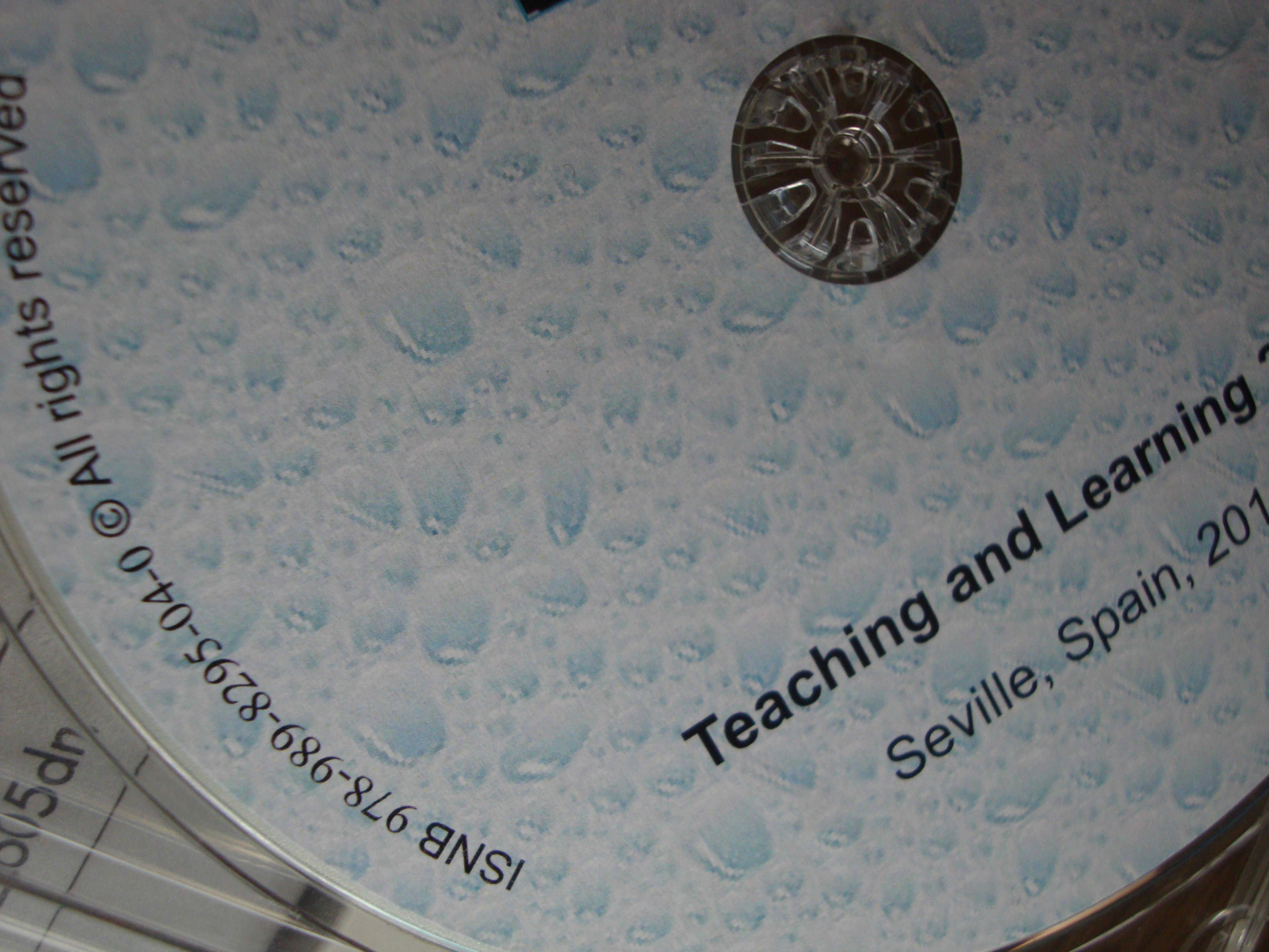
In order to visualize a new algorithm the interface is simple to use: an existing Octave algorithm must be selected via a specific interface (see Fig. 1). At the same time the input values for this mathematical algorithm are introduced using that interface.

Fig. 1. The display is done first by the choice of the algorithm and by the declaration of input parameters.

T

————————————————

� Carlos Balsa is with the Polytechnic Institute of Bragança, apartado 1134, 5301-857 Bragança, Portugal: E-mail: balsa@ipb.pt.

� Luís Alves is with the Polytechnic Institute of Bragança, apartado 1134, 5301-857 Bragança, Portugal: E-mail: lalves@ipb.pt.

� Maria J. Varanda Pereira is with the Polytechnic Institute of Bragança, apartado 1134, 5301-857 Bragança, Portugal: E-mail: mjoao@ipb.pt

� Pedro J. Rodrigues is with the Polytechnic Institute of Bragança, apartado 1134, 5301-857 Bragança, Portugal: E-mail: pjsr@ipb.pt.

IASK TL2010 CONFERENCE PROCEEDINGS

- 595 -

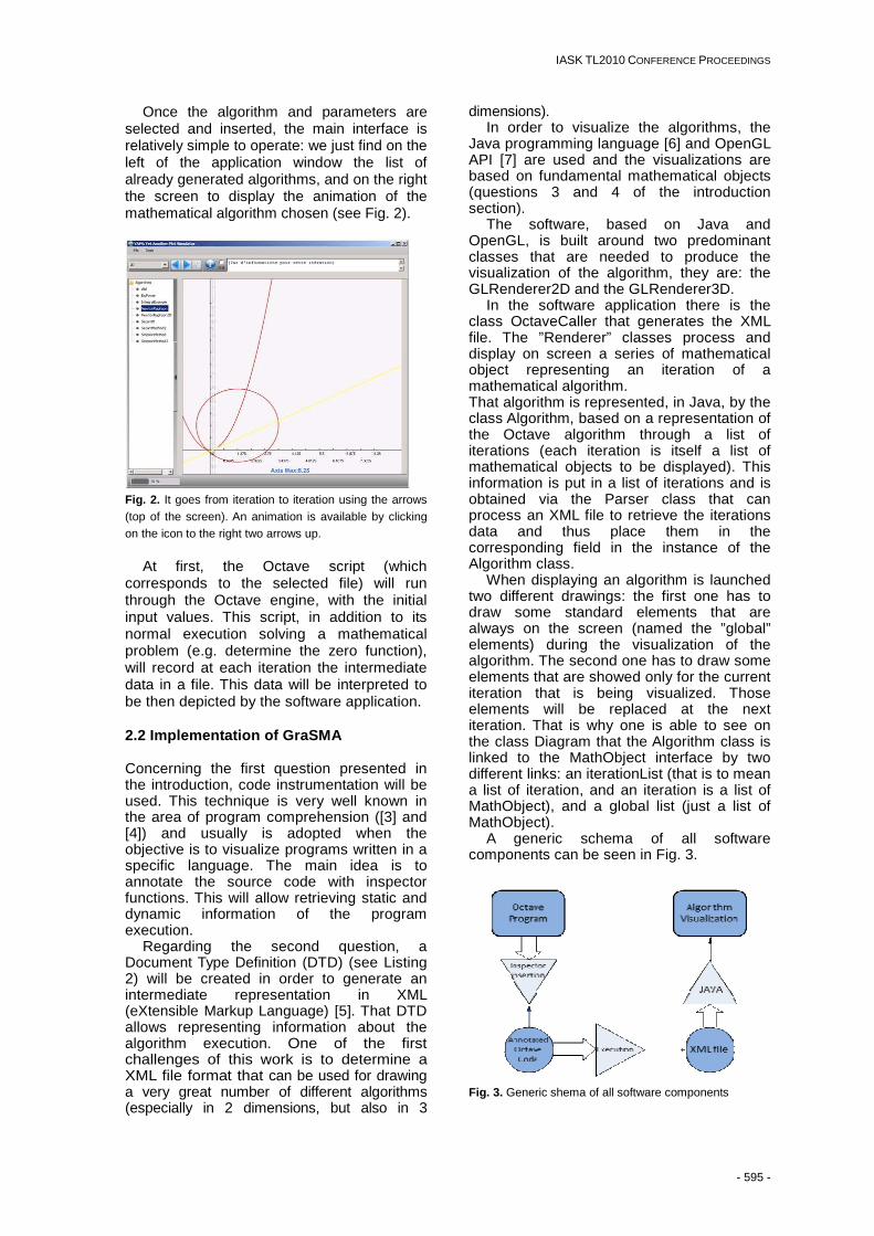
Once the algorithm and parameters are selected and inserted, the main interface is relatively simple to operate: we just find on the left of the application window the list of already generated algorithms, and on the right the screen to display the animation of the mathematical algorithm chosen (see Fig. 2).

Fig. 2. It goes from iteration to iteration using the arrows (top of the screen). An animation is available by clicking on the icon to the right two arrows up.

At first, the Octave script (which

corresponds to the selected file) will run through the Octave engine, with the initial input values. This script, in addition to its normal execution solving a mathematical problem (e.g. determine the zero function), will record at each iteration the intermediate data in a file. This data will be interpreted to be then depicted by the software application.

2.2 Implementation of GraSMA

Concerning the first question presented in the introduction, code instrumentation will be used. This technique is very well known in the area of program comprehension ([3] and [4]) and usually is adopted when the objective is to visualize programs written in a specific language. The main idea is to annotate the source code with inspector functions. This will allow retrieving static and dynamic information of the program execution.

Regarding the second question, a Document Type Definition (DTD) (see Listing 2) will be created in order to generate an intermediate representation in XML (eXtensible Markup Language) [5]. That DTD allows representing information about the algorithm execution. One of the first challenges of this work is to determine a XML file format that can be used for drawing a very great number of different algorithms (especially in 2 dimensions, but also in 3

dimensions). In order to visualize the algorithms, the

Java programming language [6] and OpenGL API [7] are used and the visualizations are based on fundamental mathematical objects (questions 3 and 4 of the introduction section).

The software, based on Java and OpenGL, is built around two predominant classes that are needed to produce the visualization of the algorithm, they are: the GLRenderer2D and the GLRenderer3D.

In the software application there is the class OctaveCaller that generates the XML file. The ”Renderer” classes process and display on screen a series of mathematical object representing an iteration of a mathematical algorithm. That algorithm is represented, in Java, by the class Algorithm, based on a representation of the Octave algorithm through a list of iterations (each iteration is itself a list of mathematical objects to be displayed). This information is put in a list of iterations and is obtained via the Parser class that can process an XML file to retrieve the iterations data and thus place them in the corresponding field in the instance of the Algorithm class.

When displaying an algorithm is launched two different drawings: the first one has to draw some standard elements that are always on the screen (named the ”global” elements) during the visualization of the algorithm. The second one has to draw some elements that are showed only for the current iteration that is being visualized. Those elements will be replaced at the next iteration. That is why one is able to see on the class Diagram that the Algorithm class is linked to the MathObject interface by two different links: an iterationList (that is to mean a list of iteration, and an iteration is a list of MathObject), and a global list (just a list of MathObject).

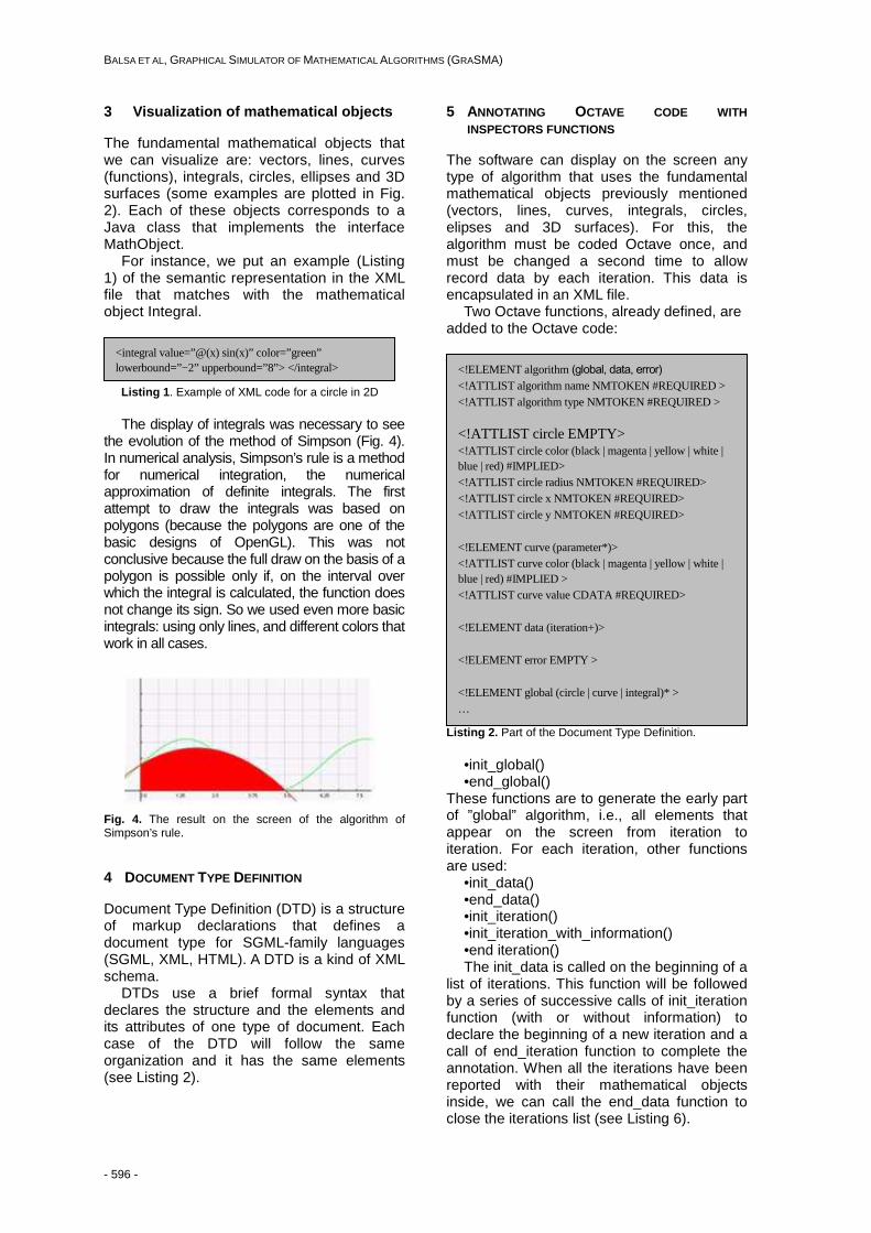
A generic schema of all software components can be seen in Fig. 3.

Fig. 3. Generic shema of all software components

BALSA ET AL, GRAPHICAL SIMULATOR OF MATHEMATICAL ALGORITHMS (GRASMA)

- 596 -

3 Visualization of mathematical objects

The fundamental mathematical objects that we can visualize are: vectors, lines, curves (functions), integrals, circles, ellipses and 3D surfaces (some examples are plotted in Fig. 2). Each of these objects corresponds to a Java class that implements the interface MathObject.

For instance, we put an example (Listing 1) of the semantic representation in the XML file that matches with the mathematical object Integral.

Listing 1 . Example of XML code for a circle in 2D The display of integrals was necessary to see

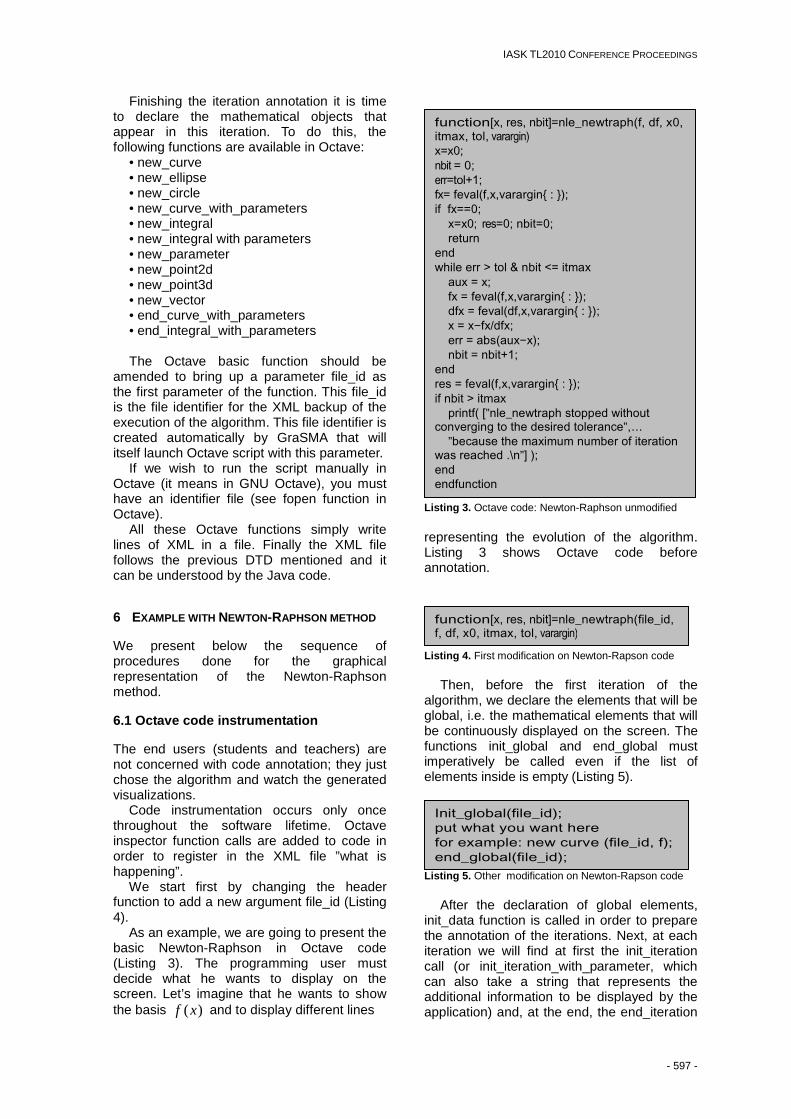
the evolution of the method of Simpson (Fig. 4). In numerical analysis, Simpson’s rule is a method for numerical integration, the numerical approximation of definite integrals. The first attempt to draw the integrals was based on polygons (because the polygons are one of the basic designs of OpenGL). This was not conclusive because the full draw on the basis of a polygon is possible only if, on the interval over which the integral is calculated, the function does not change its sign. So we used even more basic integrals: using only lines, and different colors that work in all cases.

Fig. 4. The result on the screen of the algorithm of Simpson’s rule.

4 DOCUMENT TYPE DEFINITION

Document Type Definition (DTD) is a structure of markup declarations that defines a document type for SGML-family languages (SGML, XML, HTML). A DTD is a kind of XML schema.

DTDs use a brief formal syntax that declares the structure and the elements and its attributes of one type of document. Each case of the DTD will follow the same organization and it has the same elements (see Listing 2).

5 ANNOTATING OCTAVE CODE WITH INSPECTORS FUNCTIONS

The software can display on the screen any type of algorithm that uses the fundamental mathematical objects previously mentioned (vectors, lines, curves, integrals, circles, elipses and 3D surfaces). For this, the algorithm must be coded Octave once, and must be changed a second time to allow record data by each iteration. This data is encapsulated in an XML file.

Two Octave functions, already defined, are added to the Octave code:

Listing 2. Part of the Document Type Definition. •init_global() •end_global()

These functions are to generate the early part of ”global” algorithm, i.e., all elements that appear on the screen from iteration to iteration. For each iteration, other functions are used:

•init_data() •end_data() •init_iteration() •init_iteration_with_information() •end iteration() The init_data is called on the beginning of a

list of iterations. This function will be followed by a series of successive calls of init_iteration function (with or without information) to declare the beginning of a new iteration and a call of end_iteration function to complete the annotation. When all the iterations have been reported with their mathematical objects inside, we can call the end_data function to close the iterations list (see Listing 6).

<!ELEMENT algorithm (global, data, error) <!ATTLIST algorithm name NMTOKEN #REQUIRED > <!ATTLIST algorithm type NMTOKEN #REQUIRED > <!ATTLIST circle EMPTY> <!ATTLIST circle color (black | magenta | yellow | white | blue | red) #IMPLIED> <!ATTLIST circle radius NMTOKEN #REQUIRED> <!ATTLIST circle x NMTOKEN #REQUIRED> <!ATTLIST circle y NMTOKEN #REQUIRED> <!ELEMENT curve (parameter*)> <!ATTLIST curve color (black | magenta | yellow | white | blue | red) #IMPLIED > <!ATTLIST curve value CDATA #REQUIRED> <!ELEMENT data (iteration+)> <!ELEMENT error EMPTY > <!ELEMENT global (circle | curve | integral)* > …

<integral value=”@(x) sin(x)” color=”green” lowerbound=”−2” upperbound=”8”> </integral>

IASK TL2010 CONFERENCE PROCEEDINGS

- 597 -

Finishing the iteration annotation it is time to declare the mathematical objects that appear in this iteration. To do this, the following functions are available in Octave:

• new_curve • new_ellipse • new_circle • new_curve_with_parameters • new_integral • new_integral with parameters • new_parameter • new_point2d • new_point3d • new_vector • end_curve_with_parameters • end_integral_with_parameters The Octave basic function should be

amended to bring up a parameter file_id as the first parameter of the function. This file_id is the file identifier for the XML backup of the execution of the algorithm. This file identifier is created automatically by GraSMA that will itself launch Octave script with this parameter.

If we wish to run the script manually in Octave (it means in GNU Octave), you must have an identifier file (see fopen function in Octave).

All these Octave functions simply write lines of XML in a file. Finally the XML file follows the previous DTD mentioned and it can be understood by the Java code.

6 EXAMPLE WITH NEWTON-RAPHSON METHOD

We present below the sequence of procedures done for the graphical representation of the Newton-Raphson method.

6.1 Octave code instrumentation

The end users (students and teachers) are not concerned with code annotation; they just chose the algorithm and watch the generated visualizations.

Code instrumentation occurs only once throughout the software lifetime. Octave inspector function calls are added to code in order to register in the XML file ”what is happening”.

We start first by changing the header function to add a new argument file_id (Listing 4).

As an example, we are going to present the basic Newton-Raphson in Octave code (Listing 3). The programming user must decide what he wants to display on the screen. Let’s imagine that he wants to show the basis ( )f x and to display different lines

Listing 3. Octave code: Newton-Raphson unmodified representing the evolution of the algorithm. Listing 3 shows Octave code before annotation.

Listing 4. First modification on Newton-Rapson code

Then, before the first iteration of the algorithm, we declare the elements that will be global, i.e. the mathematical elements that will be continuously displayed on the screen. The functions init_global and end_global must imperatively be called even if the list of elements inside is empty (Listing 5).

Listing 5. Other modification on Newton-Rapson code After the declaration of global elements,

init_data function is called in order to prepare the annotation of the iterations. Next, at each iteration we will find at first the init_iteration call (or init_iteration_with_parameter, which can also take a string that represents the additional information to be displayed by the application) and, at the end, the end_iteration

function[x, res, nbit]=nle_newtraph(file_id, f, df, x0, itmax, tol, varargin)

function[x, res, nbit]=nle_newtraph(f, df, x0, itmax, tol, varargin) x=x0; nbit = 0; err=tol+1; fx= feval(f,x,varargin{ : }); if fx==0; x=x0; res=0; nbit=0; return end while err > tol & nbit <= itmax aux = x; fx = feval(f,x,varargin{ : }); dfx = feval(df,x,varargin{ : }); x = x−fx/dfx; err = abs(aux−x); nbit = nbit+1; end res = feval(f,x,varargin{ : }); if nbit > itmax printf( [”nle_newtraph stopped without converging to the desired tolerance”,… ”because the maximum number of iteration was reached .\n”] ); end endfunction

Init_global(file_id); put what you want here for example: new curve (file_id, f); end_global(file_id);

BALSA ET AL, GRAPHICAL SIMULATOR OF MATHEMATICAL ALGORITHMS (GRASMA)

- 598 -

function call. All these functions (which records data in

an XML file) have always as first parameter file_id. After the end of the list of iterations, a call to end_data function is necessary.

Finally, it remains only to make a call to init_error and end_error before closing the data tag (end_data). One can put a list of errors (new_error_point) after the call to init_error. Listing 6 shows the last modification of Octave code, including all the inspector function calls needed to retrieve all the information we want to visualize.

Listing 6. Newton-Raphson code modified

6.2 Using GraSMA

At the opening of GraSMA system, 3 choices are possible:

1. Display of an algorithm that is already registered

2. Create a new view of an algorithm that is already octave changed

3. Import an existing XML file that corresponds to a previous DTD and which is therefore possible to display it on the screen.

In the case 1, you have just to click on the left list, on the algorithm, previously implemented, of your choice. In the case 3, one simply has to click on Files in the menu and then on Import to select the XML file.

In the case of creating a new view of an algorithm already changed in Octave, the process is more complex. First we select Files, then New, and it simply shows the steps on a new window. In this stage the completion of function parameters is done:

- The parameter Algorithm_Type can take any value (it is no longer necessary, this setting may therefore, in the future, never to be asked – there is just for compatibility).

- If we need to refer a function, we must think about writing this function in Octave format (for example @(x) sin(x) for the sinus function).

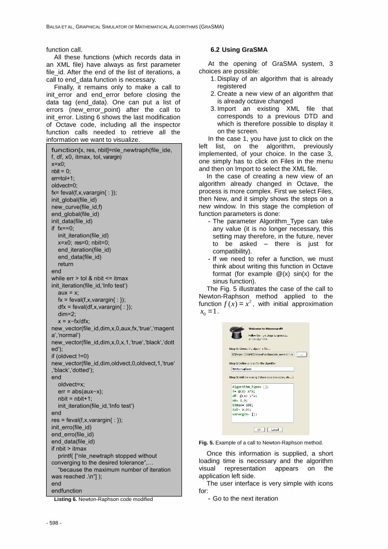
The Fig. 5 illustrates the case of the call to Newton-Raphson method applied to the function 2( )f x x= , with initial approximation

0 1x = .

Fig. 5. Example of a call to Newton-Raphson method.

Once this information is supplied, a short loading time is necessary and the algorithm visual representation appears on the application left side.

The user interface is very simple with icons for:

- Go to the next iteration

function[x, res, nbit]=nle_newtraph(file_ide, f, df, x0, itmax, tol, varargin) x=x0; nbit = 0; err=tol+1; oldvect=0; fx= feval(f,x,varargin{ : }); init_global(file_id) new_curve(file_id,f) end_global(file_id) init_data(file_id) if fx==0; init_iteration(file_id) x=x0; res=0; nbit=0; end_iteration(file_id) end_data(file_id) return end while err > tol & nbit <= itmax init_iteration(file_id,’Info test’) aux = x; fx = feval(f,x,varargin{ : }); dfx = feval(df,x,varargin{ : }); dim=2; x = x−fx/dfx; new_vector(file_id,dim,x,0,aux,fx,’true’,’magenta’,’normal’) new_vector(file_id,dim,x,0,x,1,’true’,’black’,’dotted’); if (oldvect !=0) new_vector(file_id,dim,oldvect,0,oldvect,1,’true’,’black’,’dotted’); end oldvect=x; err = abs(aux−x); nbit = nbit+1; init_iteration(file_id,’Info test’) end res = feval(f,x,varargin{ : }); init_erro(file_id) end_erro(file_id) end_data(file_id) if nbit > itmax printf( [”nle_newtraph stopped without converging to the desired tolerance”,… ”because the maximum number of iteration was reached .\n”] ); end endfunction

IASK TL2010 CONFERENCE PROCEEDINGS

- 599 -

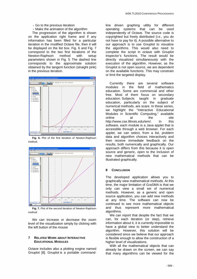
- Go to the previous iteration - Make the animation of the algorithm The progression of the algorithm is shown

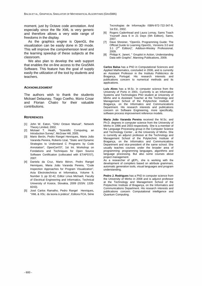
on the application right frame and if any information has been filled for a particular iteration in the modified Octave file, then it will be displayed on the list box. Fig. 6 and Fig. 7 correspond to the two first iterations of the Newton-Raphson method with setup parameters shown in Fig. 5. The dashed line corresponds to the approximate solution obtained by the tangent function (straight pink) in the previous iteration.

Fig. 6. Plot of the first iteration of Newton-Raphson method.

Fig. 7. Plot of the second iteration of Newton-Raphson method

We can increase or decrease the zoom

level of the visualization simply by clicking with the left button of the mouse

7 RELATED WORK ABOUT INTERACTIVE EDUCATIONAL MODULES

Octave includes also a plotting engine named Gnuplot [8]. Gnuplot is a portable command-

line driven graphing utility for different operating systems that can be used independently of Octave. The source code is copyrighted but freely distributed (i.e., you do not have to pay for it). A possible alternative to our approach is to use Gnuplot to visualize the algorithms. This would also need to complete the script in octave with Gnuplot inspector’s functions. The result would be directly visualized simultaneously with the execution of the algorithm. However, as the Gnuplot is not open source, we are dependent on the available functions. This may constrain or limit the targeted display.

Currently there are several software modules in the field of mathematics education. Some are commercial and other free. Most of them focus on secondary education. Subjects taught in graduate education, particularly on the subject of numerical methods, are scare. In these series, we highlight the "Interactive Educational Modules in Scientific Computing," available online at the site http://www.cse.illinois.edu/iem/. In this software, each module is a Java applet that is accessible through a web browser. For each applet, we can select, from a list, problem data and algorithm choices interactively and then receive immediate feedback on the results, both numerically and graphically. Our approach differs from this because it is open source and generic, open to the inclusion of new mathematical methods that can be illustrated graphically.

8 CONCLUSION

The developed application allows you to graphically view mathematical methods. At this time, the major limitation of GraSMA is that we only can view a small set of numerical methods. However, as a generic and open source application, you can add new methods at any time. The software can now be continued to see more mathematical objects and thus represent more mathematical algorithms.

We can report that despite the fact that we can, for each iteration (or step), retrieve information about it, it is currently impossible to have a global view to better understand the algorithm. However, this solution will be considered since we believe that our approach is flexible enough to allow the construction of a higher level of visualizations.

With all the mathematical objects that can already be drawn on the screen, we can say that many algorithms can be viewed for the

BALSA ET AL, GRAPHICAL SIMULATOR OF MATHEMATICAL ALGORITHMS (GRASMA)

- 600 -

moment, just by Octave code annotation. And especially since the file XML is very generic and therefore allows a very wide range of freedoms in the display.

As the graphics engine is OpenGL the visualization can be easily done in 3D mode. This will improve the comprehension level and the learning speedup of these subjects at the classroom.

We also plan to develop the web support that enables the on-line access to the GraSMA Software. This feature has the goal of supply easily the utilization of the tool by students and teachers.

ACKNOWLEDGMENT

The authors wish to thank the students Mickael Delaunay, Tiago Coelho, Mário César and Florian Chatré for their valuable contributions.

REFERENCES

[1] John W. Eaton, "GNU Octave Manual", Network Theory Limited, 2002.

[2] Mickael T. Heath, “Scientific Computing, an Introduction Survey”, McGraw Hill, 2005.

[3] Mario Berón, Pedro Rangel Henriques, Maria João Varanda Pereira, Roberto Uzal, "Static and Dynamic Strategies to Understand C Programs by Code Annotation", OpenCert'07, 1st Int. Workshop on Fondations and Techniques for Open Source Software Certification (collocated with ETAPS'07), 2007.

[4] Daniela da Cruz, Mario Béron, Pedro Rangel Henriques, Maria João Varanda Pereira, "Code Inspection Approaches for Program Visualization", Acta Electrotechnica et Informatica, Volume 9, Number 3, pp 32-42, Editor Linus Michaeli, Faculty of Electrical Engineering and Informatics, Technical University of Kosice, Slovakia, 2009 (ISSN: 1335-8243).

[5] José Carlos Ramalho, Pedro Rangel Henriques, "XML & XSL: da teoria à prática", Editora FCA, Série

Tecnologias de Informação ISBN-972-722-347-8, 1st Ed., 2002.

[6] Rogers Cadenhead and Laura Lemay, Sams Teach Yourself Java 6 in 21 Days (5th Edition), Sams, 2007.

[7] Dave Shreiner, “OpenGL Programming Guide: The Official Guide to Learning OpenGL, Versions 3.0 and 3.1 (7th Edition)”, Addison-Wesley Professional, 2009.

[8] Philipp K. Janert, " Gnuplot in Action, Understanding Data with Graphs”, Manning Publications, 2009.

Carlos Balsa has a PhD in Computational Sciences and Applied Mathematics, concluded in 2006, and is currently an Assistant Professor in the Instituto Politécnico de Bragança, Portugal. His research interests and publications concern to numerical methods and its applications. Luís Alves has a M.Sc. in computer science from the University of Porto in 2001. Currently is an Information Systems and Technologies PhD student at University of Minho and is Assistant Teacher at the Technology and Management School of the Polytechnic Institute of Bragança, on the Informatics and Communications Department. His research interests and publications concern on Software Engineering, more specifically, software process improvement reference models. Maria João Varanda Pereira received the M.Sc. and Ph.D. degrees in computer science from the University of Minho in 1996 and 2003 respectively. She is a member of the Language Processing group in the Computer Science and Technology Center , at the University of Minho. She is currently an adjunct professor at the Technology and Management School of the Polytechnic Institute of Bragança, on the Informatics and Communications Department and vice-president of the same school. She usually teaches courses under the broader area of programming: programming languages, algorithms and language processing. But also some courses about project management. As a researcher of gEPL, she is working with the development of compilers based on attribute grammars, automatic generation tools, visual languages and program understanding. Pedro J. Rodrigues has a PhD in computer science from the University of Minho in 2008 and is adjunct professor at the Technology and Management School of the Polytechnic Institute of Bragança, on the Informatics and Communications Department. His research interests and publications concern Computational intelligence and Quantum Computing.