Chapter 5 Mathematical Model of Excavator DiggingAs depicted in the VR excavator simulator architecture, the mathematical model of excavator digging (or physics-based soil model of

68

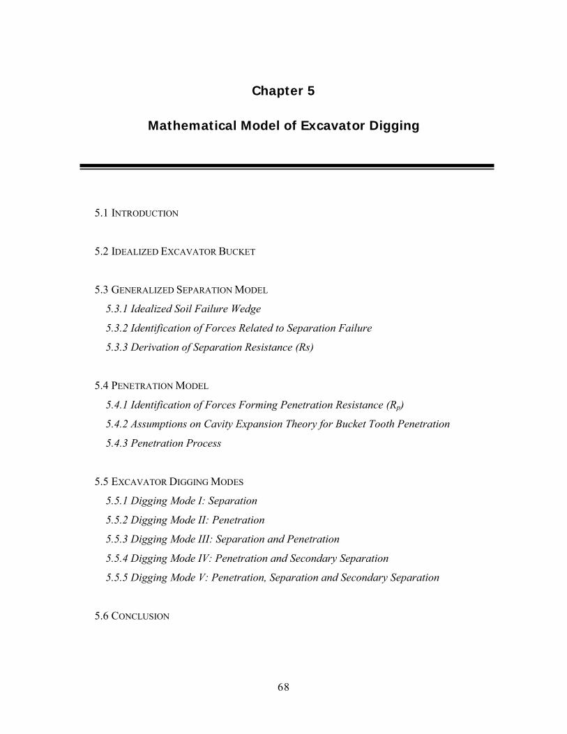
Chapter 5

Mathematical Model of Excavator Digging

5.1 INTRODUCTION

5.2 IDEALIZED EXCAVATOR BUCKET

5.3 GENERALIZED SEPARATION MODEL

5.3.1 Idealized Soil Failure Wedge

5.3.2 Identification of Forces Related to Separation Failure

5.3.3 Derivation of Separation Resistance (Rs)

5.4 PENETRATION MODEL

5.4.1 Identification of Forces Forming Penetration Resistance (Rp)

5.4.2 Assumptions on Cavity Expansion Theory for Bucket Tooth Penetration

5.4.3 Penetration Process

5.5 EXCAVATOR DIGGING MODES

5.5.1 Digging Mode I: Separation

5.5.2 Digging Mode II: Penetration

5.5.3 Digging Mode III: Separation and Penetration

5.5.4 Digging Mode IV: Penetration and Secondary Separation

5.5.5 Digging Mode V: Penetration, Separation and Secondary Separation

5.6 CONCLUSION

69

Chapter 5

Mathematical Model of Excavator Digging

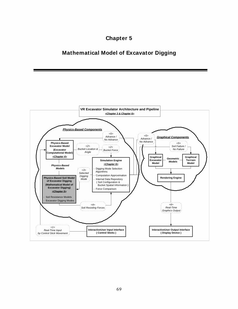
Physics-Based Components

Simulation Engine<Chapter 6>

- Digging Mode Selection Algorithms - Computation Approximation - Internal Data Repository ( Soil Configuration & Bucket Spatial Information ) - Force Comparison

InteractiveUser Input Interface( Control Sticks )

<4>Soil Resisting Forces

Graphical Components

Rendering Engine

GraphicalExcavator

Model

GraphicalTerrrainModel

InteractiveUser Output Interface( Display Device )

<6>Real-Time

Graphics Output

Physics-BasedExcavator Model

(ExcavatorComputational Model)

<Chapter 4>

Physics-Based Soil Modelof Excavator Digging

(Mathematical Model ofExcavator Digging)

<Chapter 5>

- Soil Resistance Models - Excavator Digging Modes

<2>Bucket Location &

Angle

<2>Bucket Force

VR Excavator Simulator Architecture and Pipeline<Chapter 3 & Chapter 6>

Physics-BasedModels

GeometricModels

<5>Advance /

No Advance

<3>SelectedDiggingMode

<5>Advance /

No Advance <5>Soil Failure /No Failure

<1>Real-Time Input

by Control Stick Movement

70

5.1 Introduction

As depicted in the VR excavator simulator architecture, the mathematical model of

excavator digging (or physics-based soil model of excavator digging) functions as an

external medium to regulate the behavior of an excavator. Specifically it provides soil

resistance forces to the excavator computational model (or physics-based excavator

model) through the simulation engine so that physically valid movement of a bucket

through soil medium is achieved.

Three different digging mechanisms (penetration, separation, and secondary

separation) are identified in Chapter 2 as the basic instruments to explain soil failure

induced by an excavator digging tool.

In this chapter, we begin by analyzing an excavator digging tool, a bucket, to

determine which bucket area or areas are accountable for particular digging mechanisms

(Section 5.2). The identified bucket areas accounting for a particular mechanism are

grouped together to form an idealized bucket part. These parts make up an idealized

bucket.

Using the idealized bucket, a partially-competent separation model and a general

purpose penetration theory, two soil resistance models for excavator digging are

developed to predict a penetration-based resistance and a separation-based resistance to

the digging tool (Section 5.3 and 5.4).

The one-mechanism-based soil resistance models are joined together to form a

complete mathematical model of excavator digging through the use of different excavator

digging modes (Section 5.5). Criteria to differentiate one digging mode from another are

described along with typical situational digging operations.

71

5.2 Idealized Excavator Bucket

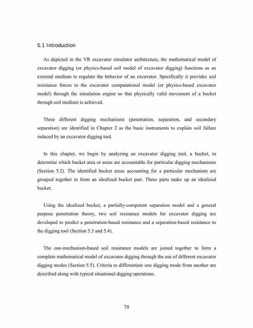
Different types of buckets used in construction excavation are shown in Figure 5.1. To

avoid extra complexity of bucket-soil interaction in mathematical modeling, it is

necessary to simplify the shape of a typical bucket.

Figure 5.1 Various Excavator Buckets Used in Construction

The steps in transforming an excavator bucket into an idealized bucket are depicted in

the diagrams of Figure 5.2 through Figure 5.4. This transformation is based on the

assumption that an excavator bucket relies on its penetration, and primary and secondary

separation forces for breaking soil. Therefore, the idealized bucket should have parts

generating these forces. The detailed description on the breakdown of each of the

separation and penetration forces into componential forces is continued in the later

sections.

72

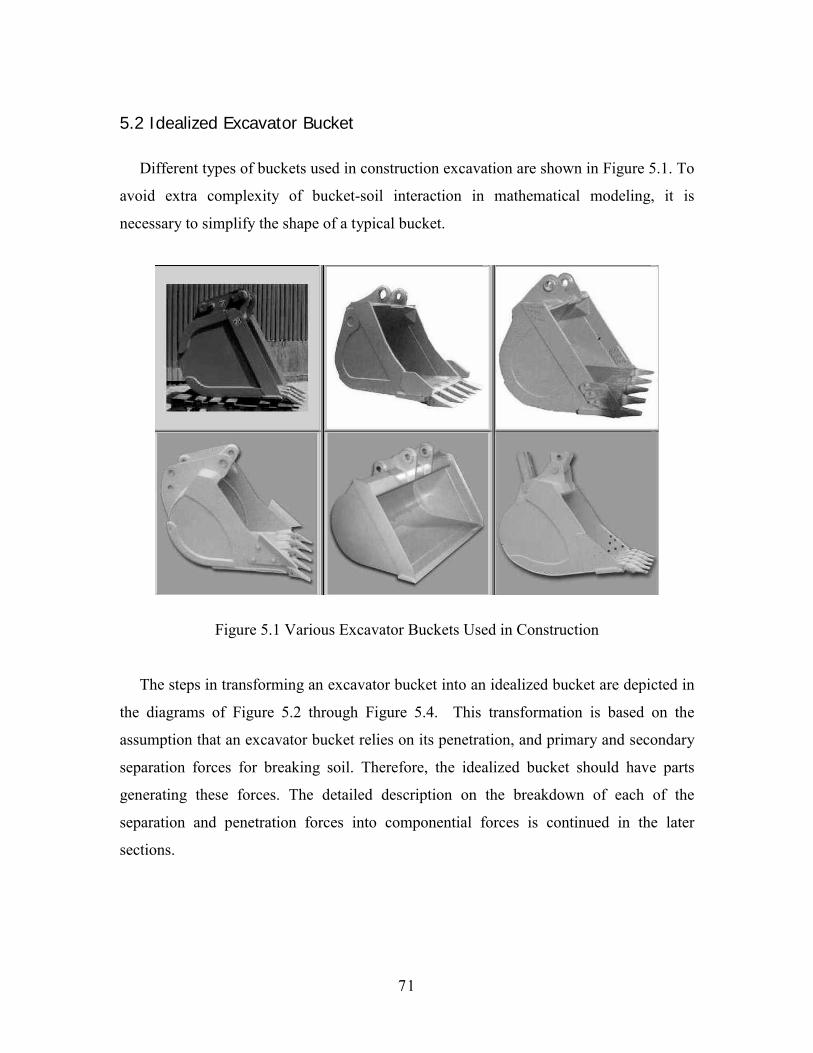
As shown in Figure 5.2, a typical bucket is comprised of 1) teeth, 2) a bottom plate,

and 3) a convex plate and side plates.

Figure 5.2 Typical Bucket: (a) Perspective View and (b) Side View

Firstly, the bucket teeth function as soil breaking parts by penetrating the media. The

shape of the tooth usually resembles a wedge form because its tapered cross-section

facilitates a penetration process by providing proper pressures continuously to push itself

into the soil media. Therefore, the shape approximation must preserve this characteristic

to be a reasonable replacement. In this regard, the wedge-shaped bucket is well

approximated by a cone-shaped tooth as shown in Figure 5.3. The dimension of this

idealized bucket tooth should be close to that of the original bucket.

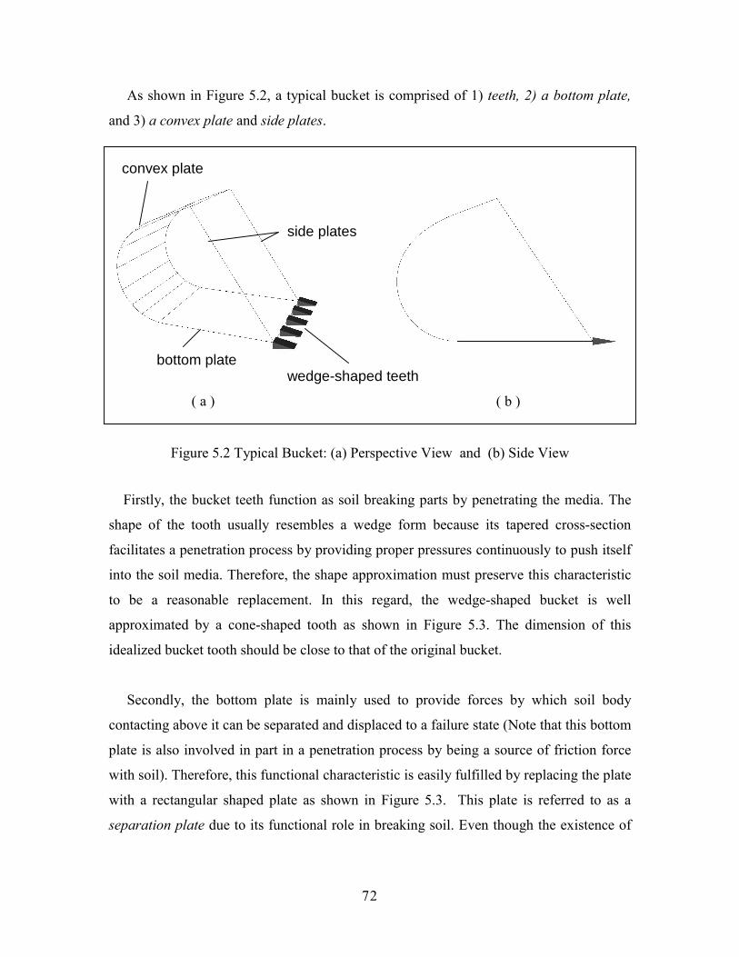
Secondly, the bottom plate is mainly used to provide forces by which soil body

contacting above it can be separated and displaced to a failure state (Note that this bottom

plate is also involved in part in a penetration process by being a source of friction force

with soil). Therefore, this functional characteristic is easily fulfilled by replacing the plate

with a rectangular shaped plate as shown in Figure 5.3. This plate is referred to as a

separation plate due to its functional role in breaking soil. Even though the existence of

( a ) ( b )

wedge-shaped teeth

side plates

convex plate

bottom plate

73

the side plates is not reflected in the simplification above, the effect of the side plates on

the separation resistance is included in the model development in the later section.

Lastly, the convex plate and the two side plates mainly contribute to the reason that

ripped soil gets filled and packed inside a bucket and eventually forms some kind of

imaginary plane by which the soil in front of it experiences additional separation failure

as described in Section 2.5. Therefore, another rectangular plate, forming a normal angle

with the separation plate, is the idealized part used to account for this lapsed separation

mechanism as shown in Figure 5.3. This plate is termed the secondary separation plate.

Figure 5.3 Bucket Overlapped with Idealized Parts:(a) Perspective View and (b) Side View

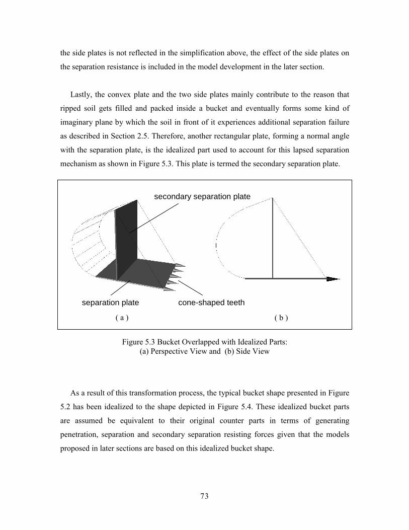
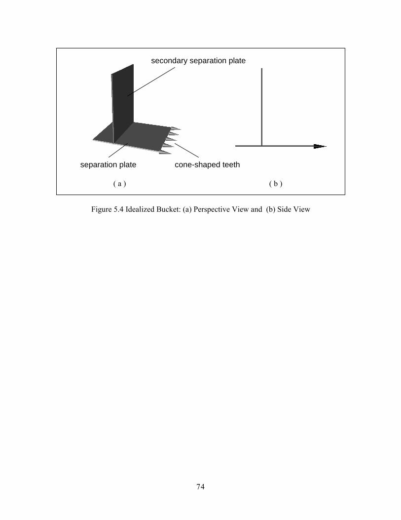
As a result of this transformation process, the typical bucket shape presented in Figure

5.2 has been idealized to the shape depicted in Figure 5.4. These idealized bucket parts

are assumed be equivalent to their original counter parts in terms of generating

penetration, separation and secondary separation resisting forces given that the models

proposed in later sections are based on this idealized bucket shape.

( a ) ( b )

separation plate

secondary separation plate

cone-shaped teeth

74

Figure 5.4 Idealized Bucket: (a) Perspective View and (b) Side View

( a ) ( b )

separation plate

secondary separation plate

cone-shaped teeth

75

5.3 Generalized Separation Model

It has been discussed that 3-D analytical resistance models are better suited to explain

soil resistance induced by separation-mechanism-based excavating tool. This is because

the 3-D resistance models predict soil resistance reasonably well by analytically

representing forces involved in the soil-tool interaction with 3-dimensional soil failure

geometries whereas 2-D analytical models and the empirical models are unable to do this.

Among these 3-D resistance models, the Perumpral�s model (Perumpral, Grisso and

Desai 1983) is selected in this research as the basic model, from which the excavator

bucket separation model is developed. This 3-D analytical model is appropriate in this

separation model generalization for the following reasons:

1) it allows a relatively simple soil failure shape without relying on experimental

results; and

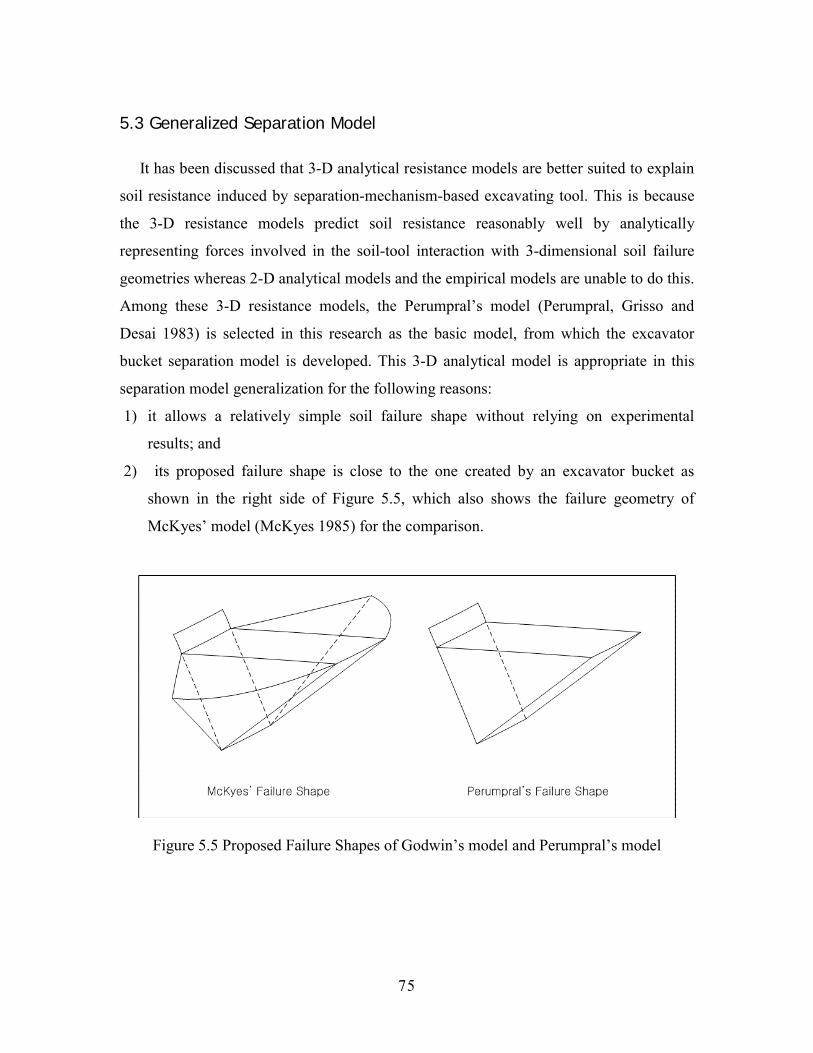
2) its proposed failure shape is close to the one created by an excavator bucket as

shown in the right side of Figure 5.5, which also shows the failure geometry of

McKyes� model (McKyes 1985) for the comparison.

Figure 5.5 Proposed Failure Shapes of Godwin�s model and Perumpral�s model

76

However, Perumpral�s model needs to be expanded such that it can predict separation

soil resistance in an inclined terrain, which is an usual terrain condition in excavator

digging cases. The model also needs to incorporate excavator bucket shape, specifically

the two side plates since the Perumpral�s model is based on a rectangular plate without

side plates. To this end, a generalized separation model is developed using the same

analytical method used in the Perumpral�s model.

5.3.1 Idealized Soil Failure Wedge

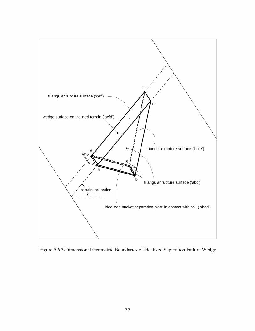
The generalized separation model starts from a 3-dimensional idealized soil failure

wedge (Figure 5.6) consisting of an idealized bucket separation plate in contact with soil

( � abed � ), a terrain surface ( � acfd � ), two triangular side rupture surfaces ( � abc � and �

def � ) and a rectangular failure surface ( � bcfe � ). This shape of the failure wedge is

similar to that used in Perumpral�s model except for the inclusion of an inclined terrain

surface. The other difference is that Perumpral�s model implicitly assumes crescentic soil

failure on tool sides as shown in the left side of Figure 5.5 and replaces it with two

triangular failure surfaces: however, in this generalized separation model for an excavator

bucket, the two side failure planes ( � abc � and � def � ) themselves are a legitimate

approximation to the actual soil rupture created by a bucket with two side plates.

77

d

a

b

c

e

f

wedge surface on inclined terrain ('acfd')

triangular rupture surface ('abc')

triangular rupture surface ('def')

triangular rupture surface ('bcfe')

terrain inclination

idealized bucket separation plate in contact with soil ('abed')

Figure 5.6 3-Dimensional Geometric Boundaries of Idealized Separation Failure Wedge

78

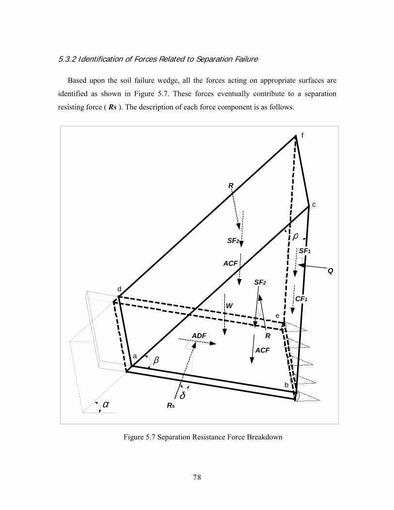
5.3.2 Identification of Forces Related to Separation Failure

Based upon the soil failure wedge, all the forces acting on appropriate surfaces are

identified as shown in Figure 5.7. These forces eventually contribute to a separation

resisting force ( Rs ). The description of each force component is as follows.

Rs

QSF2

ACF

ADF

a

b

c

d

e

f

δ

β

α

W

SF2

ACF

R

R

CF1

SF1

ρ

Figure 5.7 Separation Resistance Force Breakdown

79

Where,

! Rs : separation resisting force consisting of a parallel friction and a normal force to

the surface �abed�

! ADF : adhesional force acting on the surface �abed� due to the adhesion between the

plate and the soil

! W : gravitational force of the soil wedge

! Q : normal force acting on the rectangular failure surface �bcfe�

! SF1 : frictional force acting on the rectangular failure surface �bcfe� due to the friction

between soil particles on the interface = Q . tanΦ

! CF1 : cohesional force acting on the rectangular failure surface �bcfe� due to the

cohesion between soil particles

! R : equal and opposite normal force acting on the triangular side failure surface �abc�

or �def �

! SF2 : frictional force acting on the triangular side failure surface �abc� or �def � due to

the friction between soil particles on the interface

! ACF : adhesional-cohesional force acting on the triangular side failure surface �abc�

or �def � due to the adhesion between the side plates and the soil and the cohesion

between soil particles

! α : angle between the inclined terrain surface and the horizontal plane

! β : angle between the separation plate and the inclined terrain surface

! ρ : angle between the soil failure plane and the inclined terrain surface (soil failure

angle)

! δ : soil-metal friction angle

! Φ : soil internal friction angle

In order to include the contribution of the bucket side plates to the resistance in the

separation process, the adhesional-cohesional forces (ACF) on the triangular failure

surfaces have been included. This is different from Perumpral�s model, which

80

includes only the cohesional force. With this force included, the idealized shape of a

bucket doesn�t need to have the side plates as shown in Figure 5.7.

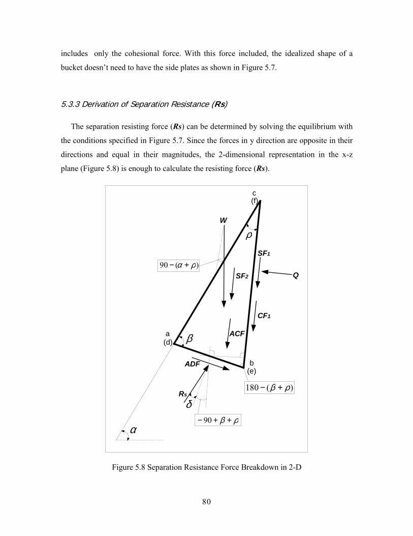
5.3.3 Derivation of Separation Resistance (Rs)

The separation resisting force (Rs) can be determined by solving the equilibrium with

the conditions specified in Figure 5.7. Since the forces in y direction are opposite in their

directions and equal in their magnitudes, the 2-dimensional representation in the x-z

plane (Figure 5.8) is enough to calculate the resisting force (Rs).

ρ

β

α

W

ADF

δRs

Q

SF1

CF1

SF2

ACFa

b

c

(d)

(e)

(f)

)(90 ρα +−

)(180 ρβ +−

ρβ ++− 90

Figure 5.8 Separation Resistance Force Breakdown in 2-D

81

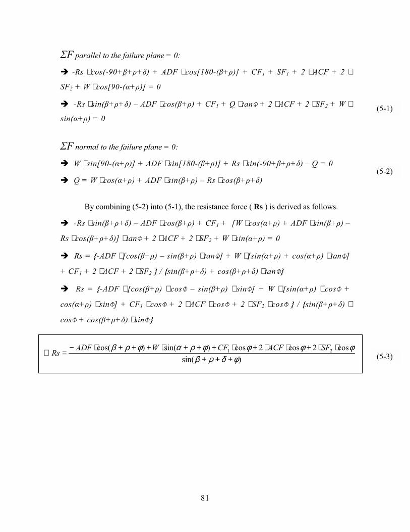
ΣF parallel to the failure plane = 0:

" -Rs ⋅ cos(-90+β+ρ+δ) + ADF ⋅ cos[180-(β+ρ)] + CF1 + SF1 + 2 ⋅ ACF + 2 ⋅

SF2 + W ⋅ cos[90-(α+ρ)] = 0

" -Rs ⋅ sin(β+ρ+δ) � ADF ⋅ cos(β+ρ) + CF1 + Q ⋅ tanΦ + 2 ⋅ ACF + 2 ⋅ SF2 + W ⋅

sin(α+ρ) = 0

ΣF normal to the failure plane = 0:

" W ⋅ sin[90-(α+ρ)] + ADF ⋅ sin[180-(β+ρ)] + Rs ⋅ sin(-90+β+ρ+δ) � Q = 0

" Q = W ⋅ cos(α+ρ) + ADF ⋅ sin(β+ρ) � Rs ⋅ cos(β+ρ+δ)

By combining (5-2) into (5-1), the resistance force ( Rs ) is derived as follows.

" -Rs ⋅ sin(β+ρ+δ) � ADF ⋅ cos(β+ρ) + CF1 + [W ⋅ cos(α+ρ) + ADF ⋅ sin(β+ρ) �

Rs ⋅ cos(β+ρ+δ)] ⋅ tanΦ + 2 ⋅ ACF + 2 ⋅ SF2 + W ⋅ sin(α+ρ) = 0

" Rs = {-ADF ⋅ [cos(β+ρ) � sin(β+ρ) ⋅ tanΦ] + W ⋅ [sin(α+ρ) + cos(α+ρ) ⋅ tanΦ]

+ CF1 + 2 ⋅ ACF + 2 ⋅ SF2 } / {sin(β+ρ+δ) + cos(β+ρ+δ) ⋅ tanΦ}

" Rs = {-ADF ⋅ [cos(β+ρ) ⋅ cosΦ � sin(β+ρ) ⋅ sinΦ] + W ⋅ [sin(α+ρ) ⋅ cosΦ +

cos(α+ρ) ⋅ sinΦ] + CF1 ⋅ cosΦ + 2 ⋅ ACF ⋅ cosΦ + 2 ⋅ SF2 ⋅ cosΦ } / {sin(β+ρ+δ) ⋅

cosΦ + cos(β+ρ+δ) ⋅ sinΦ }

)sin(cos2cos2cos)sin()cos( 21

φδρβφφφφραφρβ

+++⋅⋅+⋅⋅+⋅+++⋅+++⋅−

=∴SFACFCFWADFRs

(5-2)

(5-3)

(5-1)

82

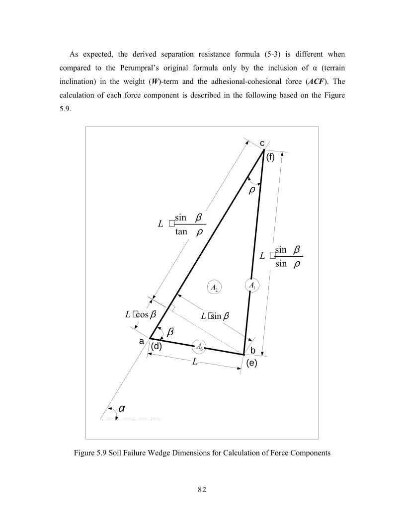
As expected, the derived separation resistance formula (5-3) is different when

compared to the Perumpral�s original formula only by the inclusion of α (terrain

inclination) in the weight (W)-term and the adhesional-cohesional force (ACF). The

calculation of each force component is described in the following based on the Figure

5.9.

ρ

β

α

ab

c

(d)

(e)

(f)

βsin⋅L

L

βcos⋅L

ρβ

tansin⋅L

ρβ

sinsin⋅L

1A2A

3A

Figure 5.9 Soil Failure Wedge Dimensions for Calculation of Force Components

83

♦ ADF = ca ⋅ A3 = ca ⋅ B ⋅ L

ca: soil adhesion

A3: area of bucket separation plate in contact with soil (�abed�)

B: separation plate width

L: length of separation plate in contact with soil

♦ W = γ ⋅ Β ⋅ Α2 = γ ⋅ Β ⋅ [0.5 ⋅ (L ⋅ sinβ) ⋅ (L ⋅ cosβ + L ⋅ sinβ / tanρ)]

= 0.5 ⋅ γ ⋅ B ⋅ L2 ⋅ sinβ ⋅ (cosβ + sinβ / tanρ)

γ: soil unit weight

Α2: area of triangular rupture surface (�abc� or �def�)

♦ CF1 = c ⋅ A1 = c ⋅ B ⋅ L ⋅ sinβ / sin ρ

c: soil cohesion

A1: area of rectangular failure surface (�bcfe�)

♦ ACF = c* ⋅ Α2 = c* ⋅ [0.5 ⋅ (L ⋅ sinβ) ⋅ (L ⋅ cosβ + L ⋅ sinβ / tanρ)]

= 0.5 ⋅ c* ⋅ L2 ⋅ sinβ ⋅ (cosβ + sinβ / tanρ)

c*: soil adhesion-cohesion

♦ SF2 = K0 ⋅ γ ⋅ z ⋅ tanΦ* ⋅ Α2

= 0.5 ⋅ K0 ⋅ γ ⋅ z ⋅ tanΦ* ⋅ L2 ⋅ sinβ ⋅ (cosβ + sinβ / tanρ)

K0 : coefficient of lateral earth pressure at rest

z: depth from the wedge top(point �c� or �f�) to the wedge centroid

Φ*: combined friction angle of δ(soil-metal friction angle) and

Φ(soil internal friction angle)

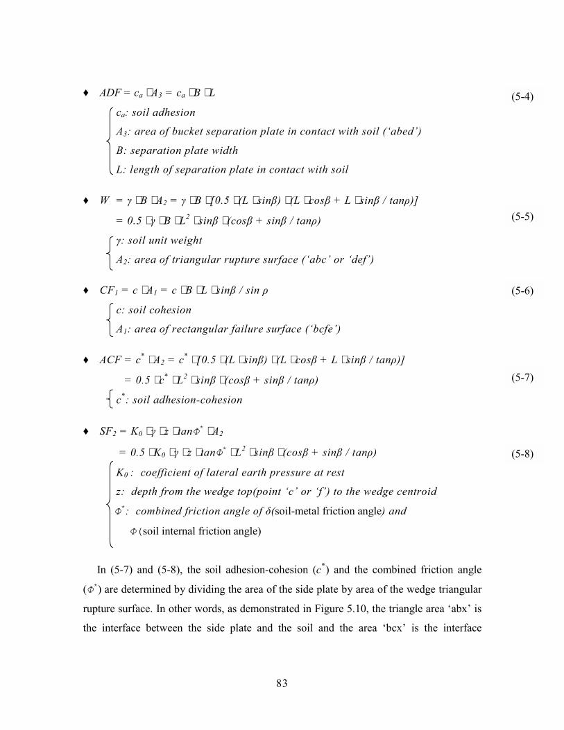
In (5-7) and (5-8), the soil adhesion-cohesion (c*) and the combined friction angle

(Φ*) are determined by dividing the area of the side plate by area of the wedge triangular

rupture surface. In other words, as demonstrated in Figure 5.10, the triangle area �abx� is

the interface between the side plate and the soil and the area �bcx� is the interface

(5-6)

(5-8)

(5-4)

(5-7)

(5-5)

84

between the soil inside the wedge and the soil outside the wedge, on which ACF and SF2

are acting. Therefore, for the area �abx�, the responsible soil properties for ACF and SF2

are the soil adhesion (ad) and the tool-soil friction angle (δ), respectively. By the same

token, for the area �bcx�, the responsible soil properties are the soil cohesion (c) and the

internal soil friction angle (Φ ) for ACF and SF2, respectively. Therefore, the soil

adhesion-cohesion (c*) and the combined friction angle (Φ*) can be determined as

follows.

Figure 5.10 Tool-soil vs. soil-soil interfaces on the side-wedge rupture surface

a b

c

x

Interface between tool and soil

Interface between soil and soil

abc

bcxabxa

AreaAreacAreacc ⋅+⋅=∗

abc

bcxabx

AreaAreaArea ⋅+⋅

=∗ φδφ (5-10)

(5-9)

85

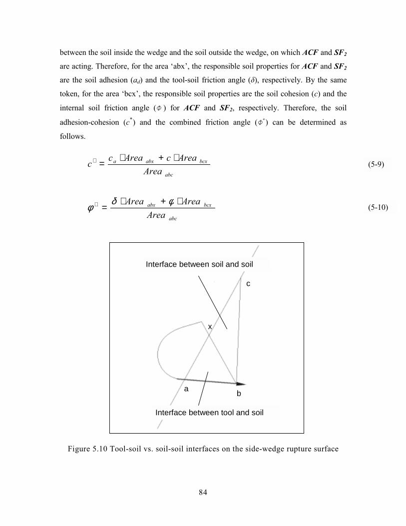
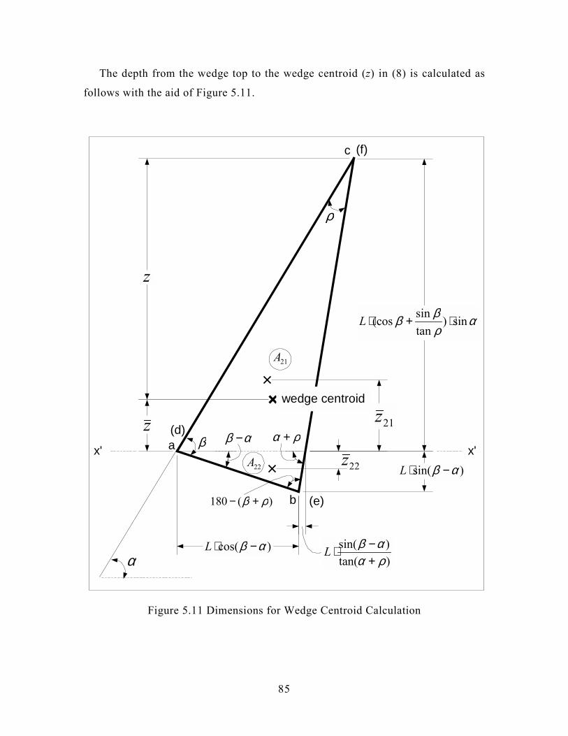
The depth from the wedge top to the wedge centroid (z) in (8) is calculated as

follows with the aid of Figure 5.11.

ρ

α

a

b

c

(d)

(e)

(f)

22A

21A

αρββ sin)

tansin(cos ⋅+⋅L

)sin( αβ −⋅L

)cos( αβ −⋅L

αβ −β ρα +

)(180 ρβ +−

x' x'

wedge centroid

z

z 21z

22z

)tan()sin(

ρααβ

+−⋅L

Figure 5.11 Dimensions for Wedge Centroid Calculation

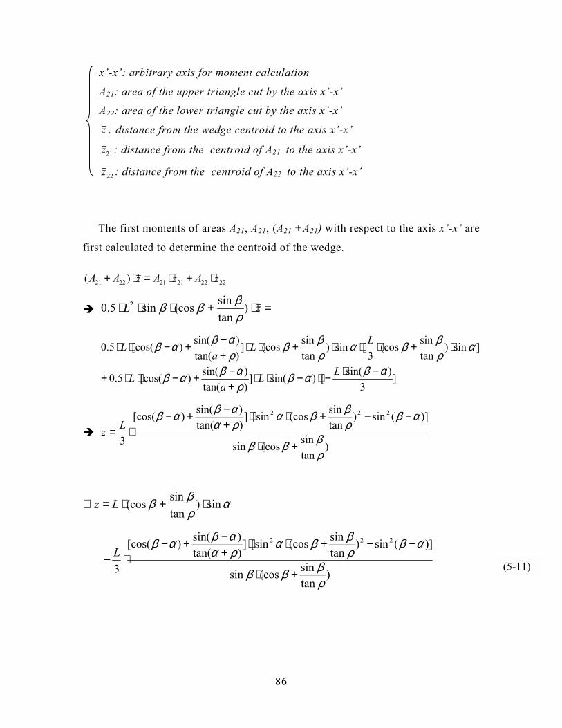
86

x�-x�: arbitrary axis for moment calculation

Α21: area of the upper triangle cut by the axis x�-x�

Α22: area of the lower triangle cut by the axis x�-x�

z : distance from the wedge centroid to the axis x�-x�

21z : distance from the centroid of Α21 to the axis x�-x�

22z : distance from the centroid of Α22 to the axis x�-x�

The first moments of areas Α21, Α21, (Α21 +Α21) with respect to the axis x�-x� are

first calculated to determine the centroid of the wedge.

222221212221 )( zAzAzAA ⋅+⋅=⋅+

" =⋅+⋅⋅⋅ zL )tansin(cossin5.0 2

ρβββ

]sin)tansin(cos

3[sin)

tansin(cos]

)tan()sin()[cos(5.0 α

ρββα

ρββ

ραβαβ ⋅+⋅⋅⋅+⋅⋅

+−+−⋅⋅ LL

aL

]3

)sin([)sin(])tan()sin()[cos(5.0 αβαβ

ραβαβ −⋅−⋅−⋅⋅

+−+−⋅⋅+ LL

aL

" )

tansin(cossin

)](sin)tansin(cos[sin]

)tan()sin()[cos(

3

222

ρβββ

αβρββα

ρααβαβ

+⋅

−−+⋅⋅+−+−

⋅= Lz

αρββ sin)

tansin(cos ⋅+⋅=∴ Lz

)

tansin(cossin

)](sin)tansin(cos[sin]

)tan()sin()[cos(

3

222

ρβββ

αβρββα

ρααβαβ

+⋅

−−+⋅⋅+−+−

⋅− L(5-11)

87

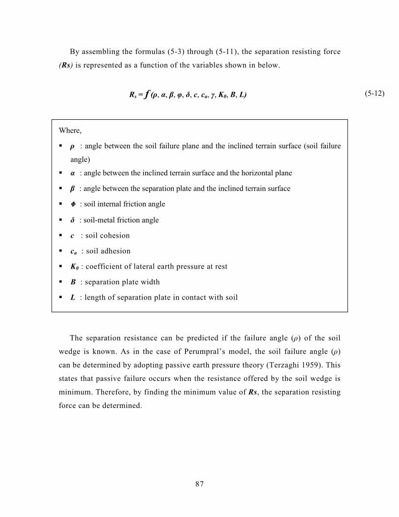
By assembling the formulas (5-3) through (5-11), the separation resisting force

(Rs) is represented as a function of the variables shown in below.

Rs = f (ρ, α, β, φ, δ, c, ca, γ, Κ0, B, L)

Where,

! ρ : angle between the soil failure plane and the inclined terrain surface (soil failure

angle)

! α : angle between the inclined terrain surface and the horizontal plane

! β : angle between the separation plate and the inclined terrain surface

! Φ : soil internal friction angle

! δ : soil-metal friction angle

! c : soil cohesion

! ca : soil adhesion

! K0 : coefficient of lateral earth pressure at rest

! B : separation plate width

! L : length of separation plate in contact with soil

The separation resistance can be predicted if the failure angle (ρ) of the soil

wedge is known. As in the case of Perumpral�s model, the soil failure angle (ρ)

can be determined by adopting passive earth pressure theory (Terzaghi 1959). This

states that passive failure occurs when the resistance offered by the soil wedge is

minimum. Therefore, by finding the minimum value of Rs, the separation resisting

force can be determined.

(5-12)

88

5.4 Penetration Model

As described in the previous section (Section 2.4.2), a penetration failure is better

explained by the cavity expansion theory than the bearing capacity theory because of its

flexibility and consistency as well as its ability to include appropriate soil behavior and

penetration process. Therefore, in this section, the cavity expansion theory is used as the

main device for determining the resistance required to penetrate soil media.

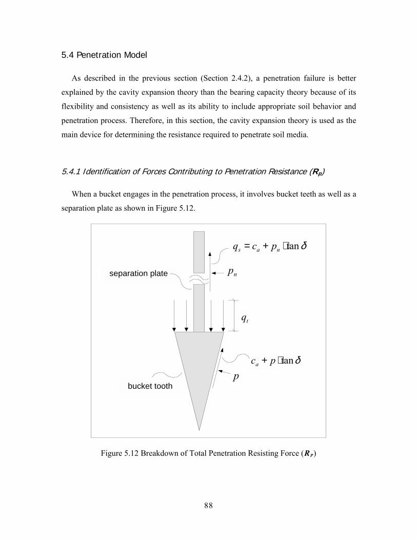
5.4.1 Identification of Forces Contributing to Penetration Resistance (Rp)

When a bucket engages in the penetration process, it involves bucket teeth as well as a

separation plate as shown in Figure 5.12.

δtan⋅+= nas pcq

np

δtan⋅+ pca

p

separation plate

bucket tooth

tq

Figure 5.12 Breakdown of Total Penetration Resisting Force (RP)

89

The total penetration resistance (Rp), therefore, consists of the resistance from the

separation plate (Rps) and the resistance from the teeth (Rpt).

ptpsp RRR +=

As shown in the Figure 5.12, the resistance Rps is comprised of adhesional (ca) and

frictional (δ) force components acting on the center of the surface of the separation plate.

The normal soil pressure (pn) on the separation plate is determined from the angle of the

separation plate in soil. When the separation plate is horizontal, pn is calculated to be γ.z

(z: depth from the surface to the centroid of the separation plate) and when the

plate is vertical in the soil, pn is Κ0 .γ.z (Κ0: coefficient of lateral earth pressure at

rest). For other cases where the separation plate is inclined, pn can be determined

by constructing a Mohr�s circle. As a result, the penetration resistance from the

separation plate (Rps) is calculated as follows.

snassps ApcAqR ⋅⋅+=⋅= )tan( δ

(As: area of the separation plate)

The resistance to penetration by the teeth (Rpt), the main quantitative target in the

penetration resistance, can be calculated from a tooth penetration pressure (qt). The tooth

penetration pressure (qt) is the equivalent of the adhesion (ca) and friction (δ) components

on the surface of the tooth as well as the cavity expansion pressure (p) itself through

which the initially small cavity grows to the size enough for the tooth to be

accommodated. Differently put, the calculation of the cavity-expansion-based tooth

penetration pressure (qt) is divided into two stages (Farrell and Greacen 1966; Ladanyi

and Johnston 1974; Yasufuku and Hyde 1995; Yu and Mitchell 1998). The first stage is

where the cavity expansion pressure (p) has increased the incipient small hole (cavity) to

the required (desired) cavity volume (with radius a). Then the second stage is where the

cavity expansion pressure (p) is linked to the tooth penetration pressure (qt).

(5-13)

(5-14)

90

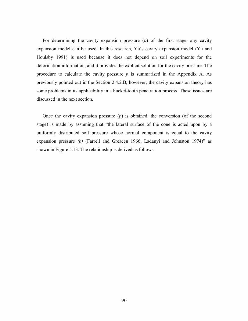
For determining the cavity expansion pressure (p) of the first stage, any cavity

expansion model can be used. In this research, Yu�s cavity expansion model (Yu and

Houlsby 1991) is used because it does not depend on soil experiments for the

deformation information, and it provides the explicit solution for the cavity pressure. The

procedure to calculate the cavity pressure p is summarized in the Appendix A. As

previously pointed out in the Section 2.4.2.B, however, the cavity expansion theory has

some problems in its applicability in a bucket-tooth penetration process. These issues are

discussed in the next section.

Once the cavity expansion pressure (p) is obtained, the conversion (of the second

stage) is made by assuming that �the lateral surface of the cone is acted upon by a

uniformly distributed soil pressure whose normal component is equal to the cavity

expansion pressure (p) (Farrell and Greacen 1966; Ladanyi and Johnston 1974)� as

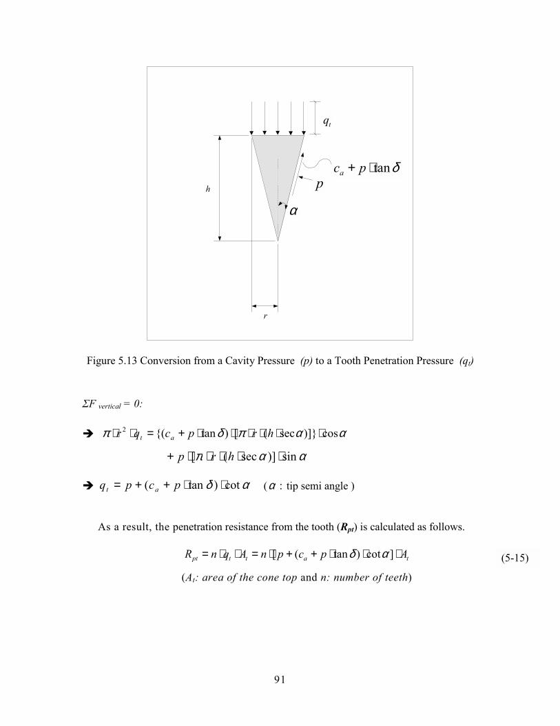
shown in Figure 5.13. The relationship is derived as follows.

91

δtan⋅+ pcap

α

tq

h

r

Figure 5.13 Conversion from a Cavity Pressure (p) to a Tooth Penetration Pressure (qt)

ΣF vertical = 0:

" ααπδπ cos)]}sec([)tan{(2 ⋅⋅⋅⋅⋅⋅+=⋅⋅ hrpcqr at

ααπ sin)]sec([ ⋅⋅⋅⋅⋅+ hrp

" αδ cot)tan( ⋅⋅++= pcpq at ( :α tip semi angle )

As a result, the penetration resistance from the tooth (Rpt) is calculated as follows.

tattpt ApcpnAqnR ⋅⋅⋅++⋅=⋅⋅= ]cot)tan([ αδ

(At: area of the cone top and n: number of teeth)

(5-15)

92

5.4.2 Assumptions on Cavity Expansion Theory for Bucket Tooth Penetration

The cavity expansion theory has some problems when it is used in bucket tooth

induced penetration cases as described in the previous section (Section 2.4.2.B). In the

following, these problems are addressed by making appropriate assumptions.

• Matching shape of bucket tooth with cavity

The cavity expansion theory assumes an ideally growing cavity in soil media either in

a spherical form or in a cylindrical form. This inherently means that the cavity expansion

pressure to form such a cavity is provided by a device whose shape is a sphere or

cylinder. Therefore the assumption creates the inevitable discrepancy between the shape

of the actual penetration tool (cone-shaped tooth) and the shape of an ideal cavity form.

Consequently, the applicability of the cavity expansion theory very much relies on how

well the bucket tooth can be matched with the cavity shape. Therefore, there should be a

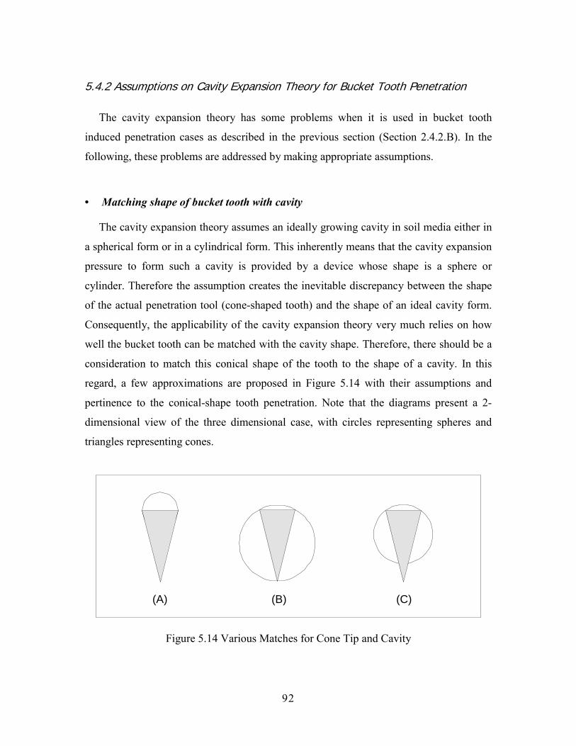
consideration to match this conical shape of the tooth to the shape of a cavity. In this

regard, a few approximations are proposed in Figure 5.14 with their assumptions and

pertinence to the conical-shape tooth penetration. Note that the diagrams present a 2-

dimensional view of the three dimensional case, with circles representing spheres and

triangles representing cones.

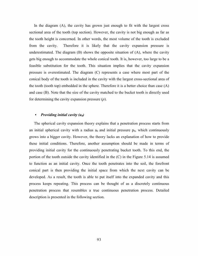
(A) (B) (C)

Figure 5.14 Various Matches for Cone Tip and Cavity

93

In the diagram (A), the cavity has grown just enough to fit with the largest cross

sectional area of the tooth (top section). However, the cavity is not big enough as far as

the tooth height is concerned. In other words, the most volume of the tooth is excluded

from the cavity. Therefore it is likely that the cavity expansion pressure is

underestimated. The diagram (B) shows the opposite situation of (A), where the cavity

gets big enough to accommodate the whole conical tooth. It is, however, too large to be a

feasible substitution for the tooth. This situation implies that the cavity expansion

pressure is overestimated. The diagram (C) represents a case where most part of the

conical body of the tooth is included in the cavity with the largest cross-sectional area of

the tooth (tooth top) embedded in the sphere. Therefore it is a better choice than case (A)

and case (B). Note that the size of the cavity matched to the bucket tooth is directly used

for determining the cavity expansion pressure (p).

• Providing initial cavity (a0)

The spherical cavity expansion theory explains that a penetration process starts from

an initial spherical cavity with a radius a0 and initial pressure p0, which continuously

grows into a bigger cavity. However, the theory lacks an explanation of how to provide

these initial conditions. Therefore, another assumption should be made in terms of

providing initial cavity for the continuously penetrating bucket tooth. To this end, the

portion of the tooth outside the cavity identified in the (C) in the Figure 5.14 is assumed

to function as an initial cavity. Once the tooth penetrates into the soil, the forefront

conical part is then providing the initial space from which the next cavity can be

developed. As a result, the tooth is able to put itself into the expanded cavity and this

process keeps repeating. This process can be thought of as a discretely continuous

penetration process that resembles a true continuous penetration process. Detailed

description is presented in the following section.

94

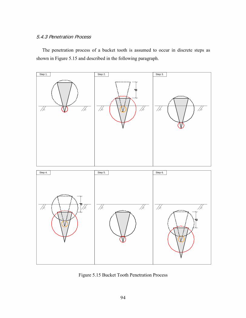
5.4.3 Penetration Process

The penetration process of a bucket tooth is assumed to occur in discrete steps as

shown in Figure 5.15 and described in the following paragraph.

Step 1. Step 2. Step 3.

Step 4. Step 5. Step 6.

d

d

d

Figure 5.15 Bucket Tooth Penetration Process

95

In the step 1, the bucket tooth is about to penetrate into the soil. The initial cavity

marked by a red circle is the space occupied by the tip of the tooth. The initial cavity

pressure (p0) is assumed to be the earth pressure at rest with the depth corresponding to

the radius a0 of the initial cavity. As the tooth is being pushed downward (step 2), this

initial cavity starts to grow and expand until it gets to a required size marked by a red

circle. At this step, the cone has advanced as much as d. The cone tip outside the circle

(step 3) now functions as another initial cavity (a0) for the next stage. This small cavity

grows to be fully expanded for the tooth to be accommodated as shown in the step 4, in

which the tooth has advanced further to the distance d. At this point, the separation plate

above the tooth starts to go down to earth along with the tooth, which experiences just

frictional and adhesional resistance as explained earlier. In the steps 5, 6, and �, the

same cavity expansion and advancement of the cavity will be repeating until the bucket

gets to the desired depth.

Note that although the bottom edge of the rectangular plate between the teeth is

contacting the soil directly, its penetration involving the expansion phenomenon need not

be considered. That is because the cavities developed by each tooth forms the enough

plastic region around them so that soil bondage between the teeth can be assumed to be

broken.

96

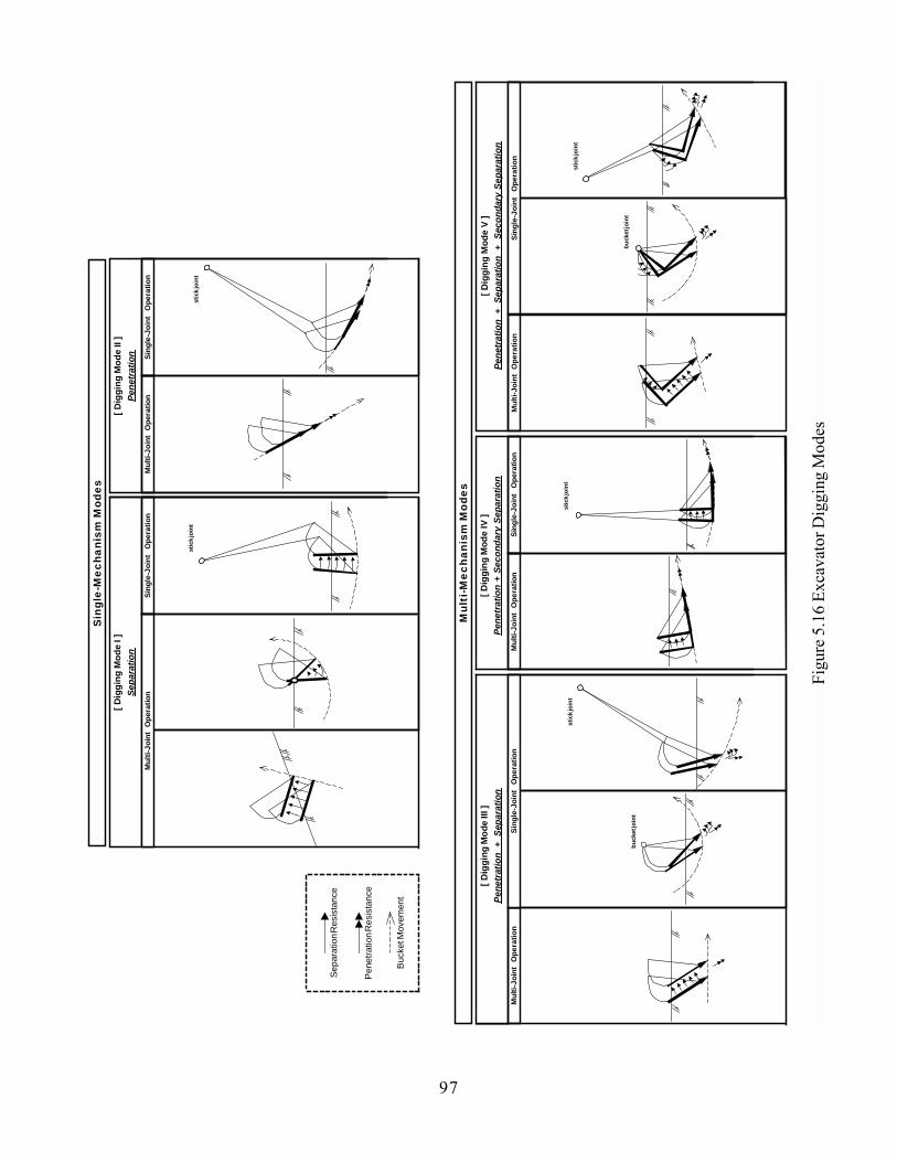
5.5 Excavator Digging Modes

Even though the separation model and the penetration model for an idealized excavator

bucket are developed, they do not represent all the possible digging actions encountered in

excavator digging because three mechanisms (separation, secondary separation and

penetration) constantly put different contributions to the generation of soil resistance in the

digging process. By virtue of the motional versatility of an excavator machine, the different

mechanisms are mixed at any stage of digging process to generate any arbitrary digging

action. To complement such a deficiency of those models, digging action groups or digging

modes are proposed in this section. The purpose of digging modes is to provide means for

any particular digging action to be classified into a certain digging situation (digging mode)

so that its underlying digging mechanism or mechanisms are identified and, therefore,

resistance for each mechanism is calculated using the models developed in the previous

sections. To serve this purpose, the digging modes represent abstracted representation for

all digging actions, whose underlying mechanisms correspond to a separation, a

penetration, a secondary separation or combination of some or all of the mechanisms. In

this section, various digging modes are explained. The conditions that constitute each

digging mode are detailed with the aid of some exemplary digging actions. All digging

modes are presented in Figure 5.16 and the description of each digging mode follows.

Note that these digging modes are the classification of the findings through small-scale

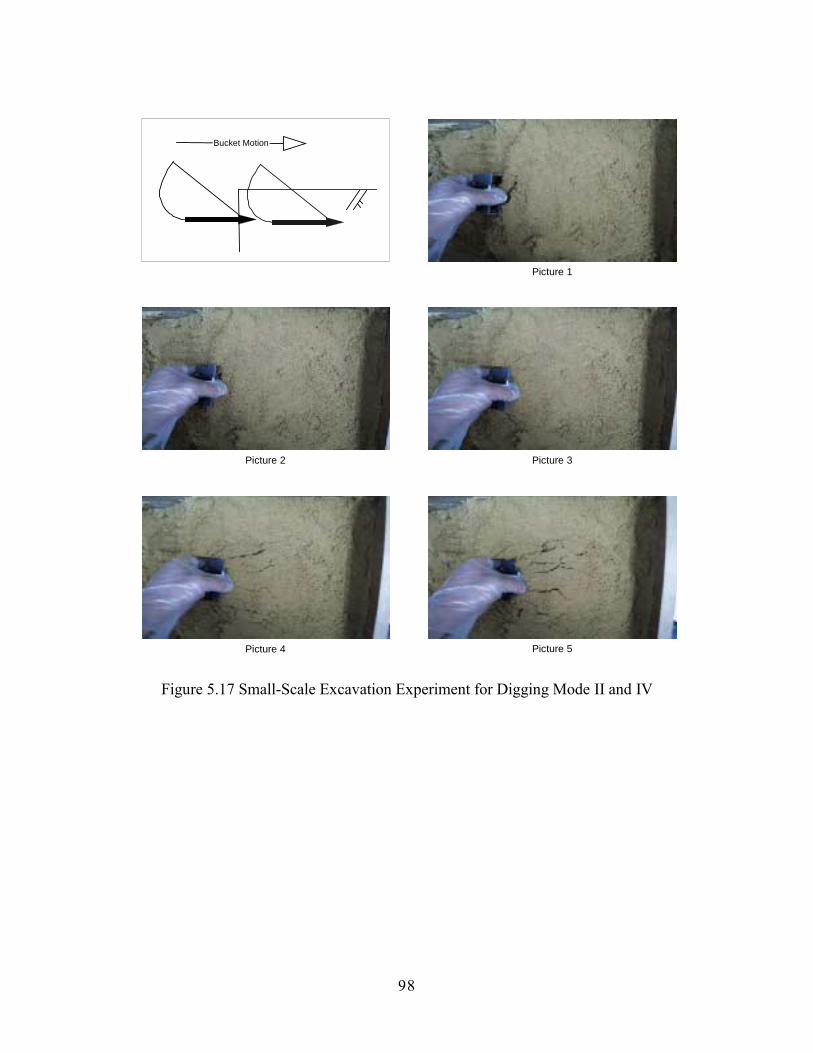
excavation experiments, and motion analyses of excavation video clips and pictures. Figure

5.17, for example, shows a series of pictures taken from a small-scale excavation

experiment, in which two digging modes are observed. In picture 1, the bucket is

introduced into the soil horizontally as shown in the upper diagram. At this stage, the

bucket only experiences the penetration resistance from the soil (digging mode II:

penetration). In picture 2, the bucket is still in the digging mode II. However, as the bucket

proceeds further in picture 3, it experiences additional resistance (secondary separation) on

the top of the penetration resistance (digging mode IV: penetration + secondary separation).

The last pictures (4 and 5) show the failure shape of the soil in the digging IV. Further

explanation on the secondary separation is included in Section 2.6.

97

Sin

gle-

Mec

hani

sm M

odes

Mul

ti-M

echa

nism

Mod

es

[ Dig

ging

Mod

e I ]

Sepa

ratio

n

Mul

ti-Jo

int

Ope

ratio

nSi

ngle

-Joi

nt

Ope

ratio

n

stic

k joi

nt

[ Dig

ging

Mod

e II

]Pe

netr

atio

nM

ulti-

Join

t O

pera

tion

stic

k joi

nt

Sing

le-J

oint

O

pera

tion

[ Dig

ging

Mod

e III

]Pe

netr

atio

n +

Sep

arat

ion

Mul

ti-Jo

int

Ope

ratio

n

buck

et jo

int

Sing

le-J

oint

O

pera

tion

stic

k joi

nt

[ Dig

ging

Mod

e IV

]Pe

netr

atio

n +

Seco

ndar

y Se

para

tion

Mul

ti-Jo

int

Ope

ratio

n

stic

k joi

nt

Sing

le-J

oint

O

pera

tion

[ Dig

ging

Mod

e V

]Pe

netr

atio

n +

Sep

arat

ion

+ S

econ

dary

Sep

arat

ion

Mul

ti-Jo

int

Ope

ratio

n

buck

et jo

int

stic

k joi

nt

Sing

le-J

oint

O

pera

tion

Figu

re 5

.16

Exca

vato

r Dig

ging

Mod

es

Sepa

ratio

n Res

ista

nce

Pene

tratio

n Res

ista

nce

Buck

et M

ovem

ent

98

Bucket Motion

Picture 1

Picture 2 Picture 3

Picture 4 Picture 5

Figure 5.17 Small-Scale Excavation Experiment for Digging Mode II and IV

99

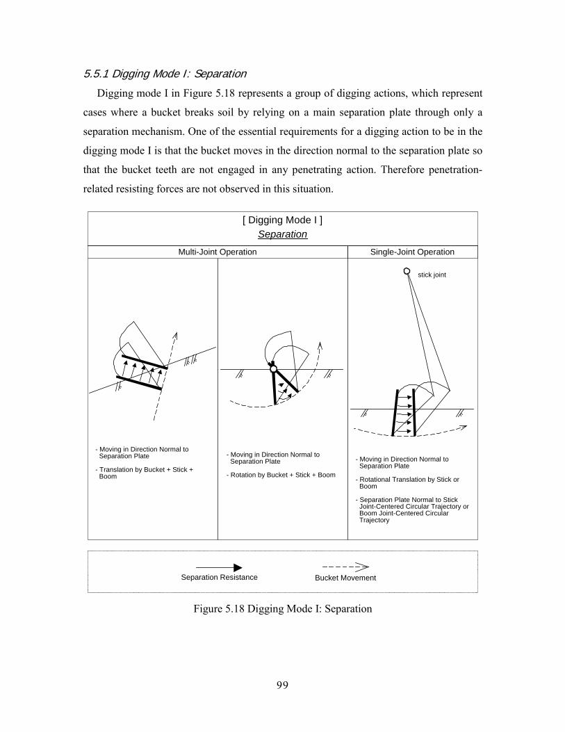
5.5.1 Digging Mode I: Separation

Digging mode I in Figure 5.18 represents a group of digging actions, which represent

cases where a bucket breaks soil by relying on a main separation plate through only a

separation mechanism. One of the essential requirements for a digging action to be in the

digging mode I is that the bucket moves in the direction normal to the separation plate so

that the bucket teeth are not engaged in any penetrating action. Therefore penetration-

related resisting forces are not observed in this situation.

[ Digging Mode I ]Separation

- Moving in Direction Normal to Separation Plate

- Translation by Bucket + Stick + Boom


- Rotation by Bucket + Stick + Boom

Multi-Joint Operation Single-Joint Operation


- Rotational Translation by Stick or Boom

- Separation Plate Normal to Stick Joint-Centered Circular Trajectory or Boom Joint-Centered Circular Trajectory

stick joint

Separation Resistance Bucket Movement

Figure 5.18 Digging Mode I: Separation

100

Depending upon driver�s operations, however, there are different motional

transformations of a separation plate. The first case in Figure 5.18 shows a situation

where a bucket makes a linear translation while maintaining its direction normal to a

separation plate. This digging motion can be achieved by simultaneously operating

multiple joints for a bucket, a stick and a boom.

The second case is when a bucket rotates itself against an arbitrary point along in a

separation plate. Even though it is rotational transformation, it meets the requirement

that every point in the separation plate maintains a normal angle to the separation plate in

its moving trajectory. Since the rotational point is not one of the mechanical joints, this

motion can be realized by manipulating a bucket, a stick and a boom together.

The last case in Figure 5.18 represents a single joint operation using either a stick joint

or a boom joint. While a bucket makes a stick joint-centered or a boom joint-centered

circular trajectory, the separation plate maintains a normal angle to the trajectory and

does not introduce penetration resistance.

5.5.2 Digging Mode II: Penetration

Figure 5.19 shows another single-mechanism mode, where bucket teeth play a major

role to penetrate into soil media and a separation plate creates some adhesion and friction

as described in the previous section. Unlike digging mode I, the direction of a bucket

movement is tangential to the separation plate and the teeth. Therefore, in this digging

mode, separation-related resisting forces are non-existent.

101

[ Digging Mode II ]Penetration

- Moving in Direction of BucketTooth


Multi-Joint Operation

stick joint

- Moving in Direction of Bucket Tooth


- Separation Plate Tangential to Stick Joint-Centered Circular Trajectory or Boom Joint-Centered Circular Trajectory

Single-Joint Operation

Penetration Resistance Bucket Movement

Figure 5.19 Digging Mode II: Penetration

The first case represents a digging operation, in which bucket teeth makes a linear

translation while meeting the tangent condition along the moving direction. This action is

possible by operating multiple joints of a bucket, a joint and a boom.

The second case shows a single-joint operation by moving either only a stick or a

boom. Even though the bucket is not making linear translation but circular trajectory, as

long as the teeth keep tangential contact with the trajectory, any operation of this type can

be classified as digging mode II.

102

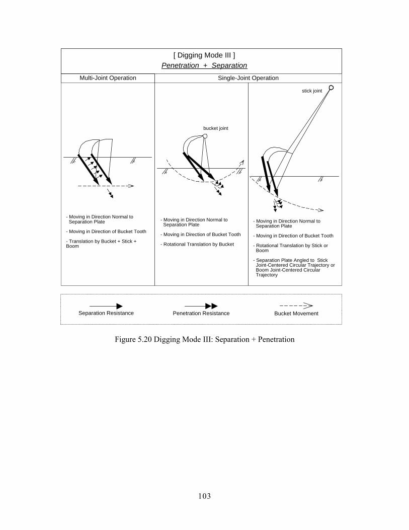
5.5.3 Digging Mode III: Separation and Penetration

Digging mode III in Figure 5.20 is a group of multi-mechanism-based digging actions,

where separation and penetration resisting forces are generated by the interaction

between soil and a separation plate and bucket teeth. This digging mode is in between

digging mode I and II in that the angle a separation plate and teeth form with the

direction of bucket movement is theoretically an arbitrary angle between 0 ~ 90o. As a

result, there are separation as well as penetration resisting forces existent in this digging

mode.

The first case shows a situation where a bucket moves in linear fashion with a

separation plate and teeth angled with the linear trajectory. The linear movement is

broken down into a normal component for separation resistance and a tangential

component for penetration resistance. This action can be made using multiple joints.

The second case is a single-joint operation using a bucket joint, where the trajectory of

a bucket tip is circular in shape. In this case, a separation plate and teeth always forms an

acute angle with the trajectory.

The third case is another single-joint operation through either a stick joint or a boom

joint. In this case a separation plate and teeth needs to maintain an acute angle with a

circular trajectory.

103

[ Digging Mode III ]Penetration + Separation



- Translation by Bucket + Stick +Boom


bucket joint



- Rotational Translation by Bucket




- Separation Plate Angled to Stick Joint-Centered Circular Trajectory or Boom Joint-Centered Circular Trajectory


stick joint

Separation Resistance Penetration Resistance Bucket Movement

Figure 5.20 Digging Mode III: Separation + Penetration

104

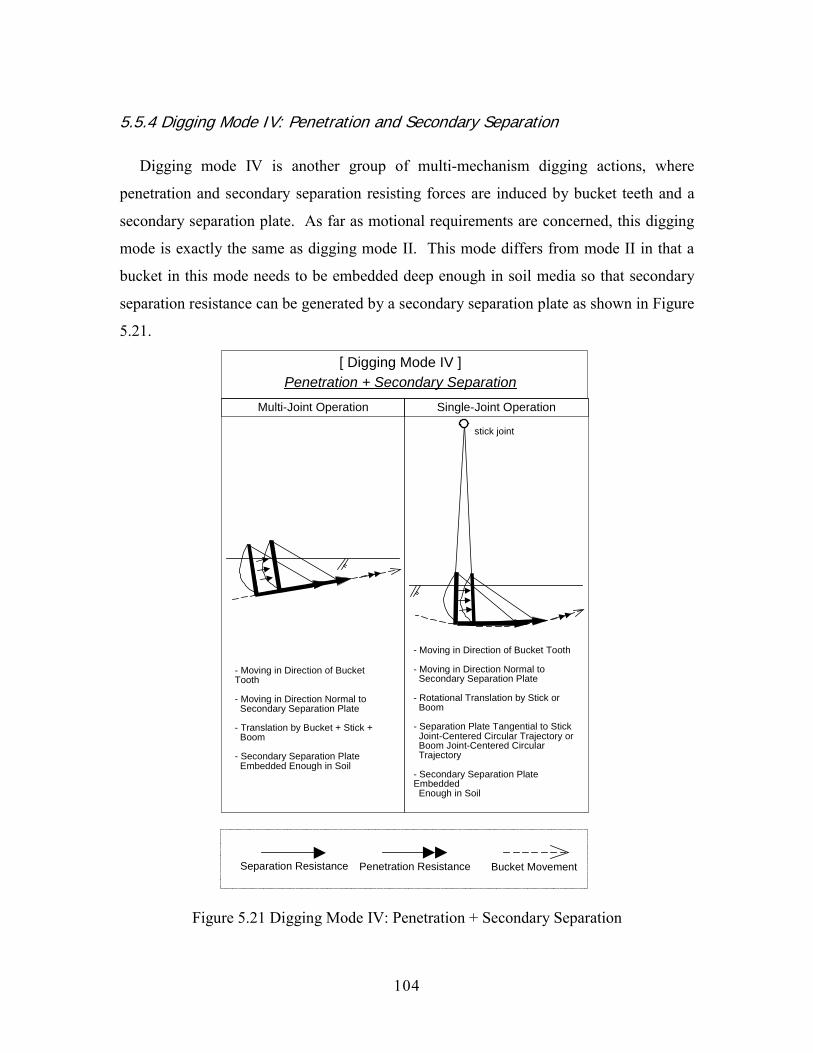
5.5.4 Digging Mode IV: Penetration and Secondary Separation

Digging mode IV is another group of multi-mechanism digging actions, where

penetration and secondary separation resisting forces are induced by bucket teeth and a

secondary separation plate. As far as motional requirements are concerned, this digging

mode is exactly the same as digging mode II. This mode differs from mode II in that a

bucket in this mode needs to be embedded deep enough in soil media so that secondary

separation resistance can be generated by a secondary separation plate as shown in Figure

5.21.

[ Digging Mode IV ]Penetration + Secondary Separation

- Moving in Direction of BucketTooth

- Moving in Direction Normal to Secondary Separation Plate


- Secondary Separation Plate Embedded Enough in Soil


stick joint




- Separation Plate Tangential to Stick Joint-Centered Circular Trajectory or Boom Joint-Centered Circular Trajectory

- Secondary Separation PlateEmbedded Enough in Soil



Figure 5.21 Digging Mode IV: Penetration + Secondary Separation

105

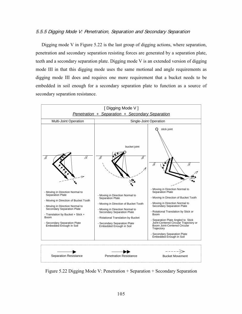
5.5.5 Digging Mode V: Penetration, Separation and Secondary Separation

Digging mode V in Figure 5.22 is the last group of digging actions, where separation,

penetration and secondary separation resisting forces are generated by a separation plate,

teeth and a secondary separation plate. Digging mode V is an extended version of digging

mode III in that this digging mode uses the same motional and angle requirements as

digging mode III does and requires one more requirement that a bucket needs to be

embedded in soil enough for a secondary separation plate to function as a source of

secondary separation resistance.

[ Digging Mode V ]Penetration + Separation + Secondary Separation




- Translation by Bucket + Stick +Boom



bucket joint




- Rotational Translation by Bucket


stick joint





- Separation Plate Angled to Stick Joint-Centered Circular Trajectory or Boom Joint-Centered Circular Trajectory




Figure 5.22 Digging Mode V: Penetration + Separation + Secondary Separation

106

5.6 Conclusion

The mathematical model of excavator digging (or physics-based soil model of

excavator digging) consists of many elements to predict soil resistance forces in an

excavator digging process. Those elements are as follows.

1) Soil resistance models:

a. Generalized separation model

b. Penetration model

2) Excavator digging modes

The idea is that any excavator digging action with a short time span is classified into

one of digging modes using the specified requirements to identify its underlying digging

mechanisms. Based upon the identification, either the generalized separation model, the

penetration model or both are used to predict resisting forces for each mechanism and to

form a total resistance by combining each resistance force. These calculated resistance

forces are used by the simulation engine when they are compared with the bucket forces

calculated from the excavator computational model (or physics-based excavator model).

Therefore, the behavior of an excavator bucket engaged in soil digging is controlled

properly in a physically meaningful way.

The description in this chapter, however, is not limited only to the development of the

VR excavator simulator system. The information is general enough to be used in other

applications. For example, an optimum digging operation practice can be determined by

comparing different resistance profiles for different operation cases and selecting the one

with the least amount of soil resistance.

Documents

Chapter 5 Mathematical Model of Excavator DiggingAs depicted in the VR excavator simulator architecture, the mathematical model of excavator digging (or physics-based soil model of