Embed Size (px)
Citation preview
SAND REPORTSAND2004-2283Unlimited ReleasePrinted June, 2004
Xyce TM Parallel ElectronicSimulator Design
Mathematical Formulation, Version 2.0
Eric R. Keiter, Scott A. Hutchinson, Robert J. Hoekstra, Thomas V. Russo, and LonJ. Waters
Prepared bySandia National LaboratoriesAlbuquerque, New Mexico 87185 and Livermore, California 94550
Sandia is a multiprogram laboratory operated by Sandia Corporation,a Lockheed Martin Company, for the United States Department ofEnergy under Contract DE-AC04-94AL85000.
Approved for public release; further dissemination unlimited.
Issued by Sandia National Laboratories, operated for the United States Department ofEnergy by Sandia Corporation.
NOTICE: This report was prepared as an account of work sponsored by an agency ofthe United States Government. Neither the United States Government, nor any agencythereof, nor any of their employees, nor any of their contractors, subcontractors, or theiremployees, make any warranty, express or implied, or assume any legal liability or re-sponsibility for the accuracy, completeness, or usefulness of any information, appara-tus, product, or process disclosed, or represent that its use would not infringe privatelyowned rights. Reference herein to any specific commercial product, process, or serviceby trade name, trademark, manufacturer, or otherwise, does not necessarily constituteor imply its endorsement, recommendation, or favoring by the United States Govern-ment, any agency thereof, or any of their contractors or subcontractors. The views andopinions expressed herein do not necessarily state or reflect those of the United StatesGovernment, any agency thereof, or any of their contractors.
Printed in the United States of America. This report has been reproduced directly fromthe best available copy.
Available to DOE and DOE contractors fromU.S. Department of EnergyOffice of Scientific and Technical InformationP.O. Box 62Oak Ridge, TN 37831
Telephone: (865) 576-8401Facsimile: (865) 576-5728E-Mail: [email protected] ordering: http://www.doe.gov/bridge
Available to the public fromU.S. Department of CommerceNational Technical Information Service5285 Port Royal RdSpringfield, VA 22161
Telephone: (800) 553-6847Facsimile: (703) 605-6900E-Mail: [email protected] ordering: http://www.ntis.gov/ordering.htm
DEP
ARTMENT OF ENERGY
• • UN
ITED
STATES OF AM
ERIC
A
SAND2004-2283Unlimited ReleasePrinted June, 2004
Xyce TM Parallel Electronic Simulator Design
Mathematical Formulation, Version 2.0
Eric R. Keiter, Scott A. Hutchinson, and Robert J. HoekstraComputational Sciences
Thomas V. Russo and Lon J. WatersComponent Information and Models
Sandia National LaboratoriesP.O. Box 5800Mail Stop 0316
Albuquerque, NM 87185-0316
Abstract
This document is intended to contain a detailed description of the mathematicalformulation of Xyce , a massively parallel SPICE-style circuit simulator developed atSandia National Laboratories. The target audience of this document are people inthe role of “service provider”. An example of such a person would be a linear solverexpert who is spending a small fraction of his time developing solver algorithms forXyce . Such a person probably is not an expert in circuit simulation, and would benefitfrom an description of the equations solved by Xyce . In this document, modified nodalanalysis (MNA) is described in detail, with a number of examples. Issues that areunique to circuit simulation, such as voltage limiting, are also described in detail.
3

Xyce TMMath Formulation
Acknowledgements
The authors would like to acknowledge the entire Sandia National Laboratories HPEMS(High Performance Electrical Modeling and Simulation) team, including Carolyn Bogdan,Regina Schells, Ken Marx, Steve Brandon, David Shirley and Bill Ballard, for their supporton this project. We also appreciate very much the work of Becky Arnold, Mike Williamson,Brett Bader and Phil Campbell for help in reviewing this document.
Trademarks
The information herein is subject to change without notice.
Copyright c© 2002-2003 Sandia Corporation. All rights reserved.
Xyce TMElectronic Simulator and Xyce TM
trademarks of Sandia Corporation.
Orcad, Orcad Capture, PSpice and Probe are registered trademarks of Cadence DesignSystems, Inc.
All other trademarks are property of their respective owners.
Contacts
Bug Reports http://tvrusso.sandia.gov/bugzillaEmail [email protected] Wide Web http://www.cs.sandia.gov/Xyce
4
CONTENTS Xyce TMMath Formulation
Contents1 Introduction . . . . . . . . . . . . . . . . . . . . . . . . . . . . . . . . . . . . . . . . . . . . . . . . . . . . . . . . . . . . . . . . . . . 92 Basics . . . . . . . . . . . . . . . . . . . . . . . . . . . . . . . . . . . . . . . . . . . . . . . . . . . . . . . . . . . . . . . . . . . . . . . . 93 Circuit Problems . . . . . . . . . . . . . . . . . . . . . . . . . . . . . . . . . . . . . . . . . . . . . . . . . . . . . . . . . . . . . . 9
3.1 Kirchhoff’s Laws . . . . . . . . . . . . . . . . . . . . . . . . . . . . . . . . . . . . . . . . . . . . . . . . . . 103.2 The modified KCL formulation . . . . . . . . . . . . . . . . . . . . . . . . . . . . . . . . . . . . . . 123.3 The “modified” part of “modified KCL” . . . . . . . . . . . . . . . . . . . . . . . . . . . . . . . . 123.4 A simple modified KCL example . . . . . . . . . . . . . . . . . . . . . . . . . . . . . . . . . . . . . 13
KCL equation for node 1: . . . . . . . . . . . . . . . . . . . . . . . . . . . . . . . . . . . . . . . . . . 14KCL equation for node 2: . . . . . . . . . . . . . . . . . . . . . . . . . . . . . . . . . . . . . . . . . . 15Voltage drop equation: . . . . . . . . . . . . . . . . . . . . . . . . . . . . . . . . . . . . . . . . . . . . . 15Linear system: . . . . . . . . . . . . . . . . . . . . . . . . . . . . . . . . . . . . . . . . . . . . . . . . . . . 15
4 Nonlinear circuits . . . . . . . . . . . . . . . . . . . . . . . . . . . . . . . . . . . . . . . . . . . . . . . . . . . . . . . . . . . . . . 174.1 Example: Nonlinear Circuit Problem . . . . . . . . . . . . . . . . . . . . . . . . . . . . . . . . . 17
KCL equation for node 1: . . . . . . . . . . . . . . . . . . . . . . . . . . . . . . . . . . . . . . . . . . 18KCL equation for node 2: . . . . . . . . . . . . . . . . . . . . . . . . . . . . . . . . . . . . . . . . . . 18Voltage drop equation: . . . . . . . . . . . . . . . . . . . . . . . . . . . . . . . . . . . . . . . . . . . . . 19Linear system: . . . . . . . . . . . . . . . . . . . . . . . . . . . . . . . . . . . . . . . . . . . . . . . . . . . 19
4.2 Voltage Limiting . . . . . . . . . . . . . . . . . . . . . . . . . . . . . . . . . . . . . . . . . . . . . . . . . . 20Voltage Limiting in Spice3f5 . . . . . . . . . . . . . . . . . . . . . . . . . . . . . . . . . . . . . . . . 21Voltage Limiting in Xyce . . . . . . . . . . . . . . . . . . . . . . . . . . . . . . . . . . . . . . . . . . . 26Additional Notes . . . . . . . . . . . . . . . . . . . . . . . . . . . . . . . . . . . . . . . . . . . . . . . . . . 28
5 Time Dependent Circuits . . . . . . . . . . . . . . . . . . . . . . . . . . . . . . . . . . . . . . . . . . . . . . . . . . . . . . 285.1 Traditional Index-1 DAE Formulation for the Linear Case . . . . . . . . . . . . . . . . . 29
KCL equation for node 1: . . . . . . . . . . . . . . . . . . . . . . . . . . . . . . . . . . . . . . . . . . 30KCL equation for node 2: . . . . . . . . . . . . . . . . . . . . . . . . . . . . . . . . . . . . . . . . . . 31Voltage drop equation: . . . . . . . . . . . . . . . . . . . . . . . . . . . . . . . . . . . . . . . . . . . . . 31Full system: . . . . . . . . . . . . . . . . . . . . . . . . . . . . . . . . . . . . . . . . . . . . . . . . . . . . . 31KCL equation for node 1: . . . . . . . . . . . . . . . . . . . . . . . . . . . . . . . . . . . . . . . . . . 31KCL equation for node 2: . . . . . . . . . . . . . . . . . . . . . . . . . . . . . . . . . . . . . . . . . . 31Voltage drop equation: . . . . . . . . . . . . . . . . . . . . . . . . . . . . . . . . . . . . . . . . . . . . . 32Full system: . . . . . . . . . . . . . . . . . . . . . . . . . . . . . . . . . . . . . . . . . . . . . . . . . . . . . 32
5.2 Traditional Index-1 DAE Formulation for the Nonlinear Case . . . . . . . . . . . . . . 335.3 Condensed DAE formulation in Xyce : State Variables . . . . . . . . . . . . . . . . . . . 35
The inexact Jacobian used with the condensed form . . . . . . . . . . . . . . . . . . . . 36Reduction in Jacobian size resulting form the condensed form . . . . . . . . . . . . 37Additional Notes . . . . . . . . . . . . . . . . . . . . . . . . . . . . . . . . . . . . . . . . . . . . . . . . . . 38
References . . . . . . . . . . . . . . . . . . . . . . . . . . . . . . . . . . . . . . . . . . . . . . . . . . . . . . . . . . . . . . . . . . . . . . . . . 40
5

Xyce TMMath Formulation
This page is left intentionally blank
6
FIGURES Xyce TMMath Formulation
Figures1 Xyce solver structure . . . . . . . . . . . . . . . . . . . . . . . . . . . . . . . . . . . . . . . . . . . . . . 102 KCL for a single circuit node. . . . . . . . . . . . . . . . . . . . . . . . . . . . . . . . . . . . . . . . 113 KVL for closed circuit loops. . . . . . . . . . . . . . . . . . . . . . . . . . . . . . . . . . . . . . . . . 114 Resistor device. . . . . . . . . . . . . . . . . . . . . . . . . . . . . . . . . . . . . . . . . . . . . . . . . . . 125 Independent voltage source. . . . . . . . . . . . . . . . . . . . . . . . . . . . . . . . . . . . . . . . . 136 Simple linear, steady-state circuit. . . . . . . . . . . . . . . . . . . . . . . . . . . . . . . . . . . . 147 Diode. . . . . . . . . . . . . . . . . . . . . . . . . . . . . . . . . . . . . . . . . . . . . . . . . . . . . . . . . . . 178 Diode I-V characteristic. . . . . . . . . . . . . . . . . . . . . . . . . . . . . . . . . . . . . . . . . . . . 189 Diode circuit . . . . . . . . . . . . . . . . . . . . . . . . . . . . . . . . . . . . . . . . . . . . . . . . . . . . . 1910 Diode circuit with resistor in parallel. . . . . . . . . . . . . . . . . . . . . . . . . . . . . . . . . . 2211 Voltage limiting flowchart. . . . . . . . . . . . . . . . . . . . . . . . . . . . . . . . . . . . . . . . . . . 2512 Linear time dependent circuit . . . . . . . . . . . . . . . . . . . . . . . . . . . . . . . . . . . . . . . 3013 MOSFET model equivalent circuit . . . . . . . . . . . . . . . . . . . . . . . . . . . . . . . . . . . 38
7

Xyce TMMath Formulation
This page is left intentionally blank
8
Xyce TMMath Formulation
1 IntroductionThis document describes how circuit problems are formulated and solved in Xyce , a mas-sively parallel analog circuit simulator. This document was motivated by the need to ad-dress common questions, asked by people new to the Xyce research/development effort.The prerequisite for understanding this document is some experience in numerical simula-tion, but not necessarily circuit simulation.
This is not intended to be an exhaustive treatment of circuit theory. What is presentedhere is a detailed summary (with examples) of how circuit problems are posed in Xyce .This includes how the problem is formulated, what equations are solved, and some of thetechniques for obtaining the solution. There are many time integration, nonlinear and linearsolver solution techniques available inside of Xyce , and most of them are not describedin this document. The solution techniques described have been limited to those for whichone or more of the following is true:
1. The technique changes the set of equations being solved.
2. The technique is (apparently) unique to circuit simulation.
3. The technique is not well described by the literature.
One such technique, voltage limiting, is described in the nonlinear solver section. Anothersuch technique, state variable condensation, is described in the time integration section.
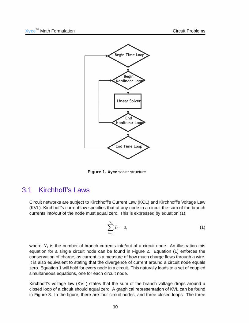
2 BasicsIf viewed abstractly, transient circuit problems are solved similarly to transient implicit partialdifferential equation (PDE) problems. There are three nested solvers: a time integrator, anonlinear solver, and a linear solver. The relationship between the three nested solvers isillustrated in Figure 1.
Like a PDE problem, a circuit problem is based upon a topology. However, unlike a PDEproblem, the topology is derived from an arbitrary circuit network connectivity, rather than amesh. As such, the circuit topologies are generally much more heterogeneous than mesh-based PDE topologies. Strang [13] describes some of the analogies between circuits andPDE problems.
3 Circuit ProblemsIn this section, Kirchhoff’s Laws, are described. Also, Modified Nodal Analysis (MNA) isintroduced. The end of this section includes a linear circuit example.
9
Xyce TMMath Formulation Circuit Problems
Figure 1. Xyce solver structure.
3.1 Kirchhoff’s Laws
Circuit networks are subject to Kirchhoff’s Current Law (KCL) and Kirchhoff’s Voltage Law(KVL). Kirchhoff’s current law specifies that at any node in a circuit the sum of the branchcurrents into/out of the node must equal zero. This is expressed by equation (1).
N1∑i=0
Ii = 0, (1)
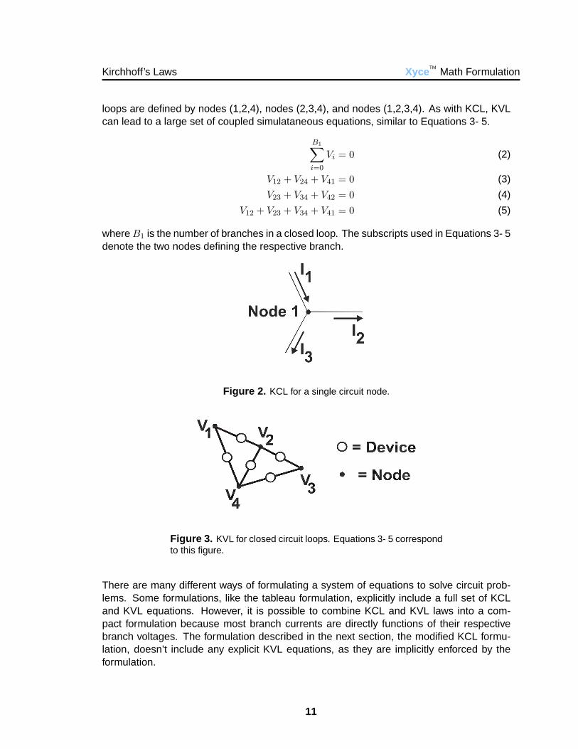
where N1 is the number of branch currents into/out of a circuit node. An illustration thisequation for a single circuit node can be found in Figure 2. Equation (1) enforces theconservation of charge, as current is a measure of how much charge flows through a wire.It is also equivalent to stating that the divergence of current around a circuit node equalszero. Equation 1 will hold for every node in a circuit. This naturally leads to a set of coupledsimultaneous equations, one for each circuit node.
Kirchhoff’s voltage law (KVL) states that the sum of the branch voltage drops around aclosed loop of a circuit should equal zero. A graphical representation of KVL can be foundin Figure 3. In the figure, there are four circuit nodes, and three closed loops. The three
10
Kirchhoff’s Laws Xyce TMMath Formulation
loops are defined by nodes (1,2,4), nodes (2,3,4), and nodes (1,2,3,4). As with KCL, KVLcan lead to a large set of coupled simulataneous equations, similar to Equations 3- 5.
B1∑i=0
Vi = 0 (2)
V12 + V24 + V41 = 0 (3)
V23 + V34 + V42 = 0 (4)
V12 + V23 + V34 + V41 = 0 (5)
where B1 is the number of branches in a closed loop. The subscripts used in Equations 3- 5denote the two nodes defining the respective branch.
Figure 2. KCL for a single circuit node.
Figure 3. KVL for closed circuit loops. Equations 3- 5 correspondto this figure.
There are many different ways of formulating a system of equations to solve circuit prob-lems. Some formulations, like the tableau formulation, explicitly include a full set of KCLand KVL equations. However, it is possible to combine KCL and KVL laws into a com-pact formulation because most branch currents are directly functions of their respectivebranch voltages. The formulation described in the next section, the modified KCL formu-lation, doesn’t include any explicit KVL equations, as they are implicitly enforced by theformulation.
11
Xyce TMMath Formulation Circuit Problems
3.2 The modified KCL formulation
Circuit problems are usually solved on a computer using the “modified KCL formulation”.This is also sometimes referred to as modified nodal analysis (MNA). This is the formulationused in all of the common circuit simulators, such as Spice3f5, as well as Xyce . Modifiednodal analysis, as well as several other types of circuit analysis, is described in detail byVlach [14] and Chua [6]. The original paper describing this technique is by Ho [12] .
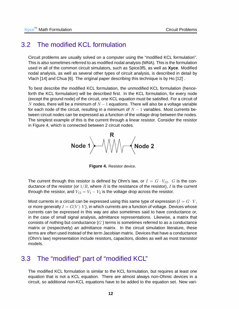
To best describe the modified KCL formulation, the unmodified KCL formulation (hence-forth the KCL formulation) will be described first. In the KCL formulation, for every node(except the ground node) of the circuit, one KCL equation must be satisfied. For a circuit ofN nodes, there will be a minimum of N − 1 equations. There will also be a voltage variablefor each node of the circuit, resulting in a minimum of N − 1 variables. Most currents be-tween circuit nodes can be expressed as a function of the voltage drop between the nodes.The simplest example of this is the current through a linear resistor. Consider the resistorin Figure 4, which is connected between 2 circuit nodes.
Figure 4. Resistor device.
The current through this resistor is defined by Ohm’s law, or I = G · V12. G is the con-ductance of the resistor (or 1/R, where R is the resistance of the resistor), I is the currentthrough the resistor, and V12 = V1 − V2 is the voltage drop across the resistor.
Most currents in a circuit can be expressed using this same type of expression (I = G · V ,or more generally I = G(V )·V ), in which currents are a function of voltage. Devices whosecurrents can be expressed in this way are also sometimes said to have conductance or,in the case of small signal analysis, admittance representations. Likewise, a matrix thatconsists of nothing but conductance (G ) terms is sometimes referred to as a conductancematrix or (respectively) an admittance matrix. In the circuit simulation literature, theseterms are often used instead of the term Jacobian matrix. Devices that have a conductance(Ohm’s law) representation include resistors, capacitors, diodes as well as most transistormodels.
3.3 The “modified” part of “modified KCL”
The modified KCL formulation is similar to the KCL formulation, but requires at least oneequation that is not a KCL equation. There are almost always non-Ohmic devices in acircuit, so additional non-KCL equations have to be added to the equation set. New vari-
12
A simple modified KCL example Xyce TMMath Formulation
ables are added to compliment these new auxiliary equations, and are generally currentvariables, rather than voltage variables.
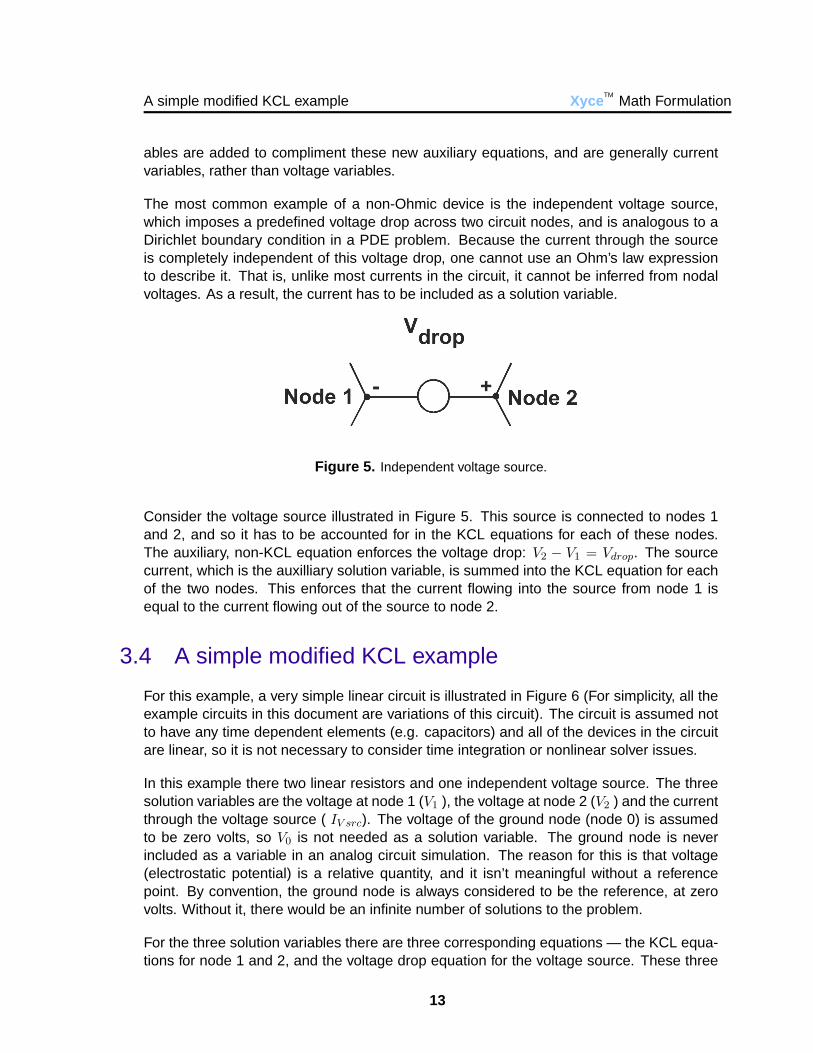
The most common example of a non-Ohmic device is the independent voltage source,which imposes a predefined voltage drop across two circuit nodes, and is analogous to aDirichlet boundary condition in a PDE problem. Because the current through the sourceis completely independent of this voltage drop, one cannot use an Ohm’s law expressionto describe it. That is, unlike most currents in the circuit, it cannot be inferred from nodalvoltages. As a result, the current has to be included as a solution variable.
Figure 5. Independent voltage source.
Consider the voltage source illustrated in Figure 5. This source is connected to nodes 1and 2, and so it has to be accounted for in the KCL equations for each of these nodes.The auxiliary, non-KCL equation enforces the voltage drop: V2 − V1 = Vdrop. The sourcecurrent, which is the auxilliary solution variable, is summed into the KCL equation for eachof the two nodes. This enforces that the current flowing into the source from node 1 isequal to the current flowing out of the source to node 2.
3.4 A simple modified KCL example
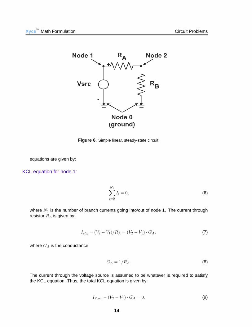
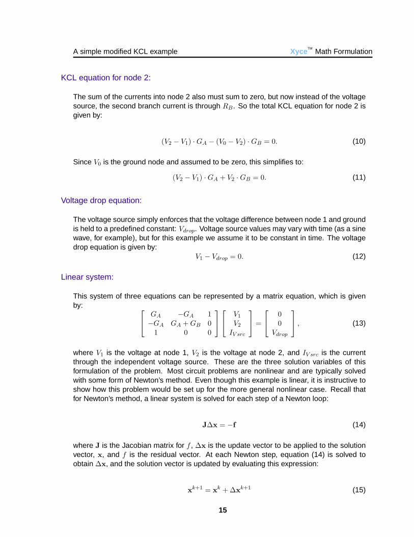
For this example, a very simple linear circuit is illustrated in Figure 6 (For simplicity, all theexample circuits in this document are variations of this circuit). The circuit is assumed notto have any time dependent elements (e.g. capacitors) and all of the devices in the circuitare linear, so it is not necessary to consider time integration or nonlinear solver issues.
In this example there two linear resistors and one independent voltage source. The threesolution variables are the voltage at node 1 (V1 ), the voltage at node 2 (V2 ) and the currentthrough the voltage source ( IV src). The voltage of the ground node (node 0) is assumedto be zero volts, so V0 is not needed as a solution variable. The ground node is neverincluded as a variable in an analog circuit simulation. The reason for this is that voltage(electrostatic potential) is a relative quantity, and it isn’t meaningful without a referencepoint. By convention, the ground node is always considered to be the reference, at zerovolts. Without it, there would be an infinite number of solutions to the problem.
For the three solution variables there are three corresponding equations — the KCL equa-tions for node 1 and 2, and the voltage drop equation for the voltage source. These three
13
Xyce TMMath Formulation Circuit Problems
Figure 6. Simple linear, steady-state circuit.
equations are given by:
KCL equation for node 1:
N1∑i=0
Ii = 0, (6)
where N1 is the number of branch currents going into/out of node 1. The current throughresistor RA is given by:
IRA= (V2 − V1)/RA = (V2 − V1) ·GA, (7)
where GA is the conductance:
GA = 1/RA. (8)
The current through the voltage source is assumed to be whatever is required to satisfythe KCL equation. Thus, the total KCL equation is given by:
IV src − (V2 − V1) ·GA = 0. (9)
14
A simple modified KCL example Xyce TMMath Formulation
KCL equation for node 2:
The sum of the currents into node 2 also must sum to zero, but now instead of the voltagesource, the second branch current is through RB. So the total KCL equation for node 2 isgiven by:
(V2 − V1) ·GA − (V0 − V2) ·GB = 0. (10)
Since V0 is the ground node and assumed to be zero, this simplifies to:
(V2 − V1) ·GA + V2 ·GB = 0. (11)
Voltage drop equation:
The voltage source simply enforces that the voltage difference between node 1 and groundis held to a predefined constant: Vdrop. Voltage source values may vary with time (as a sinewave, for example), but for this example we assume it to be constant in time. The voltagedrop equation is given by:
V1 − Vdrop = 0. (12)
Linear system:
This system of three equations can be represented by a matrix equation, which is givenby: GA −GA 1
−GA GA + GB 01 0 0
V1
V2
IV src
=
00
Vdrop
, (13)
where V1 is the voltage at node 1, V2 is the voltage at node 2, and IV src is the currentthrough the independent voltage source. These are the three solution variables of thisformulation of the problem. Most circuit problems are nonlinear and are typically solvedwith some form of Newton’s method. Even though this example is linear, it is instructive toshow how this problem would be set up for the more general nonlinear case. Recall thatfor Newton’s method, a linear system is solved for each step of a Newton loop:
J∆x = −f (14)
where J is the Jacobian matrix for f , ∆x is the update vector to be applied to the solutionvector, x, and f is the residual vector. At each Newton step, equation (14) is solved toobtain ∆x, and the solution vector is updated by evaluating this expression:
xk+1 = xk + ∆xk+1 (15)
15
Xyce TMMath Formulation Circuit Problems
where k is the step index. For the current example, the terms in ( 14, 15) are given asfollows:
f =
f1
f2
f3
=
KCL equation, node 1KCL equation, node 2
Voltage Drop constraint equation
=
IV src − (V2 − V1) ·GA
(V2 − V1) ·GA + V2 ·GB
V1 − Vdrop
(16)
J =
δf1/δV1 δf1/δV2 δf1/δIV src
δf2/δV1 δf2/δV1 δf2/δIV src
δf3/δV1 δf3/δV2 δf3/δIV src
=
GA −GA 1−GA GA + GB 0
1 0 0
(17)
∆x =
∆V1
∆V2
∆IV src
and x =
V1
V2
IV src
. (18)
Please note that the subscripts on f are meant to denote the index into the vector f . Thesubscripts on V are meant to denote the nodal index for the respective voltage. Finally,the subscripts on G are meant to refer to the resistor index. In this document, resistors willalways be denoted by letters (A, B, C) rather than numbers.
The KCL equations are current (I) equations, and their respective solution variables arevoltage (V ) variables, so most of the δf/δx terms that comprise the Jacobian matrix aregoing to be of the general form:
δf
δx=
δI
δV= G (19)
Where G is a conductance. It is only for non-Ohmic terms in f , such as the voltage sourceequation, that Jacobian elements will not be in units of conductance.
Therefore, the presence of the voltage source (which necessitates a modified KCL form)changes the structure of the Jacobian matrix, J, a great deal. There are now some non-conductance matrix contributions, which are of a fixed magnitude, 1.0. Also, the thirddiagonal element is zero. Both of these issues can result in the linear system being moredifficult to solve, but can be addressed by scaling the problem and by matrix reordering.This example illustrates part of why circuit matrices are often ill conditioned, as for a typicaldigital circuit most conductances are much smaller than 1.0. A typical conductance couldbe around 1.0e-08 or smaller. Furthermore, the respective magnitudes of the voltage andcurrent variables in the solution may be quite different (many orders of magnitude) and thisis reflected in their associated matrix entries.
As noted, in this particular example, the two resistors are linear, so the problem is solvedwith a single Newton iteration. Most circuit problems, however, have nonlinear elements,
16
Xyce TMMath Formulation
requiring multiple iterations. Some simple examples of nonlinear circuits can be found inthe next section.
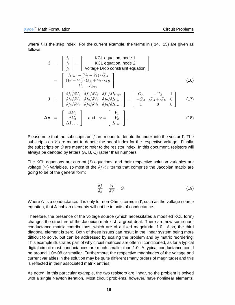
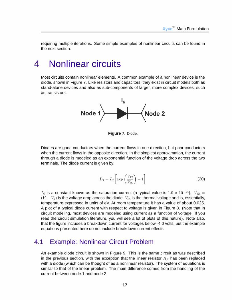
4 Nonlinear circuitsMost circuits contain nonlinear elements. A common example of a nonlinear device is thediode, shown in Figure 7. Like resistors and capacitors, they exist in circuit models both asstand-alone devices and also as sub-components of larger, more complex devices, suchas transistors.
Figure 7. Diode.
Diodes are good conductors when the current flows in one direction, but poor conductorswhen the current flows in the opposite direction. In the simplest approximation, the currentthrough a diode is modeled as an exponential function of the voltage drop across the twoterminals. The diode current is given by:
ID = IS
[exp
(V12
Vth
)− 1
](20)
IS is a constant known as the saturation current (a typical value is 1.0 × 10⁻¹⁴). V12 =(V1−V2) is the voltage drop across the diode. Vth is the thermal voltage and is, essentially,temperature expressed in units of eV. At room temperature it has a value of about 0.025.A plot of a typical diode current with respect to voltage is given in Figure 8. (Note that incircuit modeling, most devices are modeled using current as a function of voltage. If youread the circuit simulation literature, you will see a lot of plots of this nature). Note also,that the figure includes a breakdown current for voltages below -4.0 volts, but the exampleequations presented here do not include breakdown current effects.
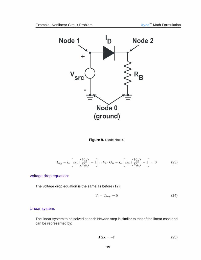
4.1 Example: Nonlinear Circuit Problem
An example diode circuit is shown in Figure 9. This is the same circuit as was describedin the previous section, with the exception that the linear resistor RA has been replacedwith a diode (which can be thought of as a nonlinear resistor). The system of equations issimilar to that of the linear problem. The main difference comes from the handling of thecurrent between node 1 and node 2.
17

Xyce TMMath Formulation Nonlinear circuits
Figure 8. Diode I-V characteristic.
KCL equation for node 1:
Recall:
N1∑i=0
Ii = 0 (21)
As before, N1 is the number of branch currents going into/out-of node 1. The currentthrough the diode is given by equation (20). The current through the voltage source, likein the previous example, is assumed to be whatever it needs to be to satisfy the KCLequation. The total KCL equation for node 1 is therefore given by:
IV src + ID = IV src + IS
[exp
(V12
Vth
)− 1
]= 0 (22)
KCL equation for node 2:
The sum of the currents into node 2 also must sum to zero, but now instead of the voltagesource, the second branch current is through RB . So the total KCL equation for node 2 isgiven by:
18
Example: Nonlinear Circuit Problem Xyce TMMath Formulation
Figure 9. Diode circuit.
IRB− IS
[exp
(V12
Vth
)− 1
]= V2 ·GB − IS
[exp
(V12
Vth
)− 1
]= 0 (23)
Voltage drop equation:
The voltage drop equation is the same as before (12):
V1 − Vdrop = 0 (24)
Linear system:
The linear system to be solved at each Newton step is similar to that of the linear case andcan be represented by:
J∆x = −f (25)
19
Xyce TMMath Formulation Nonlinear circuits
GD −GD 1−GD GD + GB 0
1 0 0
∆V1
∆V2
∆IV src
= −
IV src + IS [exp(V12/Vth)− 1]V2 ·GB − IS [exp(V12/Vth)− 1]
V1 − Vdrop
(26)
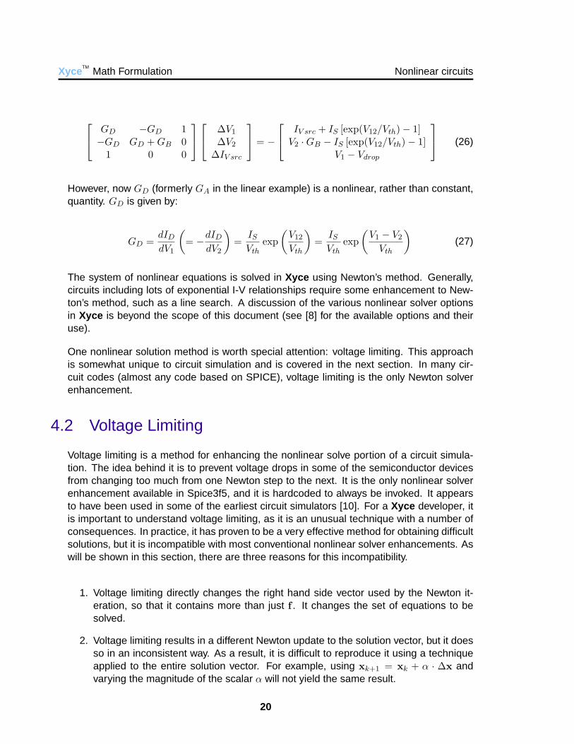
However, now GD (formerly GA in the linear example) is a nonlinear, rather than constant,quantity. GD is given by:
GD =dID
dV1
(= −dID
dV2
)=
IS
Vthexp
(V12
Vth
)=
IS
Vthexp
(V1 − V2
Vth
)(27)
The system of nonlinear equations is solved in Xyce using Newton’s method. Generally,circuits including lots of exponential I-V relationships require some enhancement to New-ton’s method, such as a line search. A discussion of the various nonlinear solver optionsin Xyce is beyond the scope of this document (see [8] for the available options and theiruse).
One nonlinear solution method is worth special attention: voltage limiting. This approachis somewhat unique to circuit simulation and is covered in the next section. In many cir-cuit codes (almost any code based on SPICE), voltage limiting is the only Newton solverenhancement.
4.2 Voltage Limiting
Voltage limiting is a method for enhancing the nonlinear solve portion of a circuit simula-tion. The idea behind it is to prevent voltage drops in some of the semiconductor devicesfrom changing too much from one Newton step to the next. It is the only nonlinear solverenhancement available in Spice3f5, and it is hardcoded to always be invoked. It appearsto have been used in some of the earliest circuit simulators [10]. For a Xyce developer, itis important to understand voltage limiting, as it is an unusual technique with a number ofconsequences. In practice, it has proven to be a very effective method for obtaining difficultsolutions, but it is incompatible with most conventional nonlinear solver enhancements. Aswill be shown in this section, there are three reasons for this incompatibility.
1. Voltage limiting directly changes the right hand side vector used by the Newton it-eration, so that it contains more than just f . It changes the set of equations to besolved.
2. Voltage limiting results in a different Newton update to the solution vector, but it doesso in an inconsistent way. As a result, it is difficult to reproduce it using a techniqueapplied to the entire solution vector. For example, using xk+1 = xk + α · ∆x andvarying the magnitude of the scalar α will not yield the same result.
20
Voltage Limiting Xyce TMMath Formulation
3. The limiting relies on the previous Newton step size, meaning that it is a function ofthe path taken to the current solution. This means that any technique using back-tracking would be subject to hysteresis.
As Xyce and Spice3f5 use different formulations for the Newton solve, there are algebraicdifferences between the two codes in voltage limiting implementation. In this section, theSpice3f5 implementation of voltage limiting will be described first, followed by a descriptionof the implementation in Xyce .
Voltage Limiting in Spice3f5
In Spice3f5, the solver solves directly for the new value of the solution at each nonlinearstep, rather than solving for the update, which is more standard for nonlinear solvers. Mosttraditional nonlinear solvers will solve this nonlinear system:
J∆xk+1 = −f (28)
∆xk+1 = xk+1 − xk (29)
The index, k, is the Newton iteration step number. In contrast, the Spice3f5 nonlineariteration is accomplished by solving this equivalent linear system:
Jxk+1 = −f + Jxk (30)
Recall that most of the elements of are nodal voltages, most of the elements of f arecurrents and most of the elements of J are in units of conductance.
Unfortunately, the Spice3f5 approach to Newton’s method means that it is impossible (orat least difficult) to apply traditional nonlinear solver libraries (such as NOX [3]). The righthand side of the Equation 30 can no longer be assumed to be −f , as it contains the Jxk
terms.
In Spice3f5, to implement voltage limiting, an analysis is performed at the beginning of eachNewton step, to determine if the previous step resulted in any junction voltage changes thatwere too large. (A junction voltage is the difference between two connected nodal voltages.An example would be a voltage drop across a diode) In the event that some of them weretoo large, portions of xi are replaced with values that are acceptable to the limiting scheme.Then after xi has been modified, the calculation proceeds as though this modified xi is thecorrect one. J and f are both calculated using this modified version of xi . In a sense, thecode goes into denial.
21
Xyce TMMath Formulation Nonlinear circuits
It should be noted that this is slightly more complicated than it may first appear, becauseall of this is done in terms of junction voltages (voltage drops between nodes), not nodalvoltages. Nodal voltages are what actually exist as distinct elements of the solution vectorxi, but junction voltages are what most devices actually care about. If we consider thediode, again, recall the expressions for diode current and the Jacobian contribution are:
ID = IS
[exp
(V12
Vth
)− 1
](31)
GD =IS
Vthexp
(V12
Vth
)(32)
Both ID and GD are functions of V12 = V1 − V2, which is a junction voltage. When acircuit code calculates the contributions of a diode to J and f , it first obtains V1 and V2
from the solution vector, and then immediately obtains V12. From that point onward in thecalculation, V1 and V2 are ignored and everything is calculated as a function of V12. This istypical in all Spice3f5-style analytical device models.
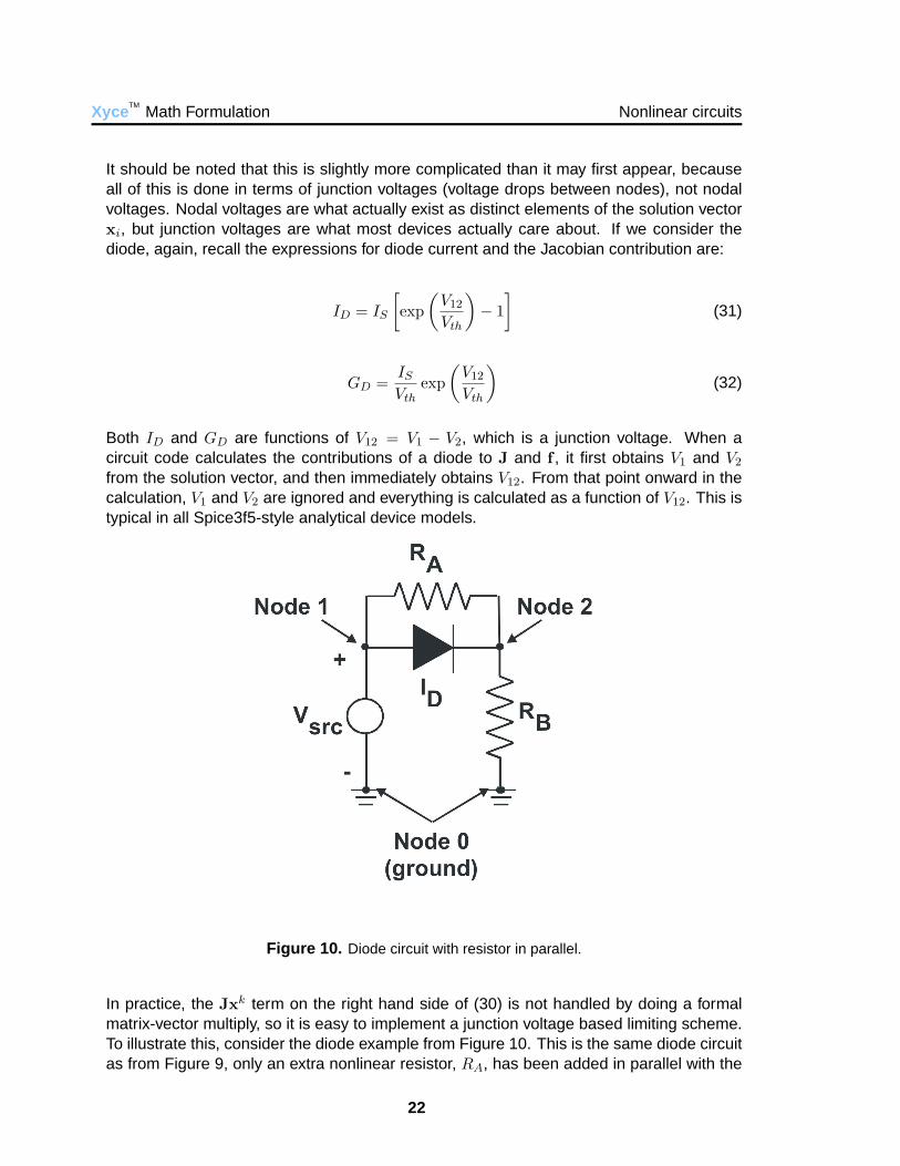
Figure 10. Diode circuit with resistor in parallel.
In practice, the Jxk term on the right hand side of (30) is not handled by doing a formalmatrix-vector multiply, so it is easy to implement a junction voltage based limiting scheme.To illustrate this, consider the diode example from Figure 10. This is the same diode circuitas from Figure 9, only an extra nonlinear resistor, RA, has been added in parallel with the
22
Voltage Limiting Xyce TMMath Formulation
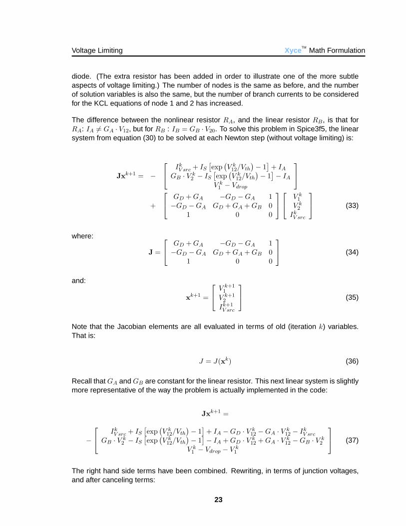
diode. (The extra resistor has been added in order to illustrate one of the more subtleaspects of voltage limiting.) The number of nodes is the same as before, and the numberof solution variables is also the same, but the number of branch currents to be consideredfor the KCL equations of node 1 and 2 has increased.
The difference between the nonlinear resistor RA, and the linear resistor RB, is that forRA: IA 6= GA · V12, but for RB : IB = GB · V20. To solve this problem in Spice3f5, the linearsystem from equation (30) to be solved at each Newton step (without voltage limiting) is:
Jxk+1 = −
IkV src + IS
[exp
(V k
12/Vth
)− 1
]+ IA
GB · V k2 − IS
[exp
(V k
12/Vth
)− 1
]− IA
V k1 − Vdrop
+
GD + GA −GD −GA 1−GD −GA GD + GA + GB 0
1 0 0
V k1
V k2
IkV src
(33)
where:
J =
GD + GA −GD −GA 1−GD −GA GD + GA + GB 0
1 0 0
(34)
and:
xk+1 =
V k+11
V k+12
Ik+1V src
(35)
Note that the Jacobian elements are all evaluated in terms of old (iteration k) variables.That is:
J = J(xk) (36)
Recall that GA and GB are constant for the linear resistor. This next linear system is slightlymore representative of the way the problem is actually implemented in the code:
Jxk+1 =
−
IkV src + IS
[exp
(V k
12/Vth
)− 1
]+ IA −GD · V k
12 −GA · V k12 − Ik
V src
GB · V k2 − IS
[exp
(V k
12/Vth
)− 1
]− IA + GD · V k
12 + GA · V k12 −GB · V k
2
V k1 − Vdrop − V k
1
(37)
The right hand side terms have been combined. Rewriting, in terms of junction voltages,and after canceling terms:
23
Xyce TMMath Formulation Nonlinear circuits
Jxk+1 = −
IS
[exp
(V k
12/Vth
)− 1
]+ IA −GD · V k
12 −GA · V k12
−IS
[exp
(V k
12/Vth
)− 1
]− IA + GD · V k
12 + GA · V k12
−Vdrop
(38)
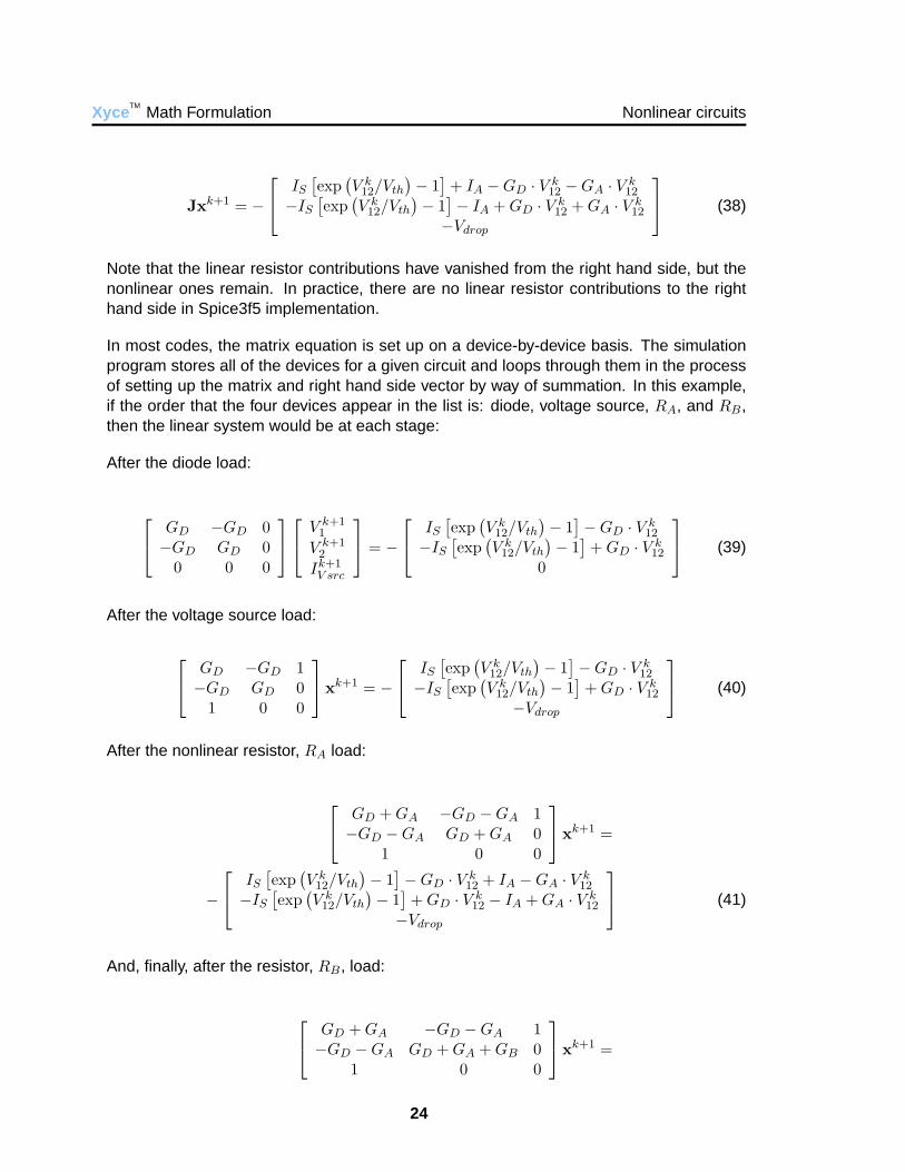
Note that the linear resistor contributions have vanished from the right hand side, but thenonlinear ones remain. In practice, there are no linear resistor contributions to the righthand side in Spice3f5 implementation.
In most codes, the matrix equation is set up on a device-by-device basis. The simulationprogram stores all of the devices for a given circuit and loops through them in the processof setting up the matrix and right hand side vector by way of summation. In this example,if the order that the four devices appear in the list is: diode, voltage source, RA, and RB,then the linear system would be at each stage:
After the diode load:
GD −GD 0−GD GD 0
0 0 0
V k+11
V k+12
Ik+1V src
= −
IS
[exp
(V k
12/Vth
)− 1
]−GD · V k
12
−IS
[exp
(V k
12/Vth
)− 1
]+ GD · V k
12
0
(39)
After the voltage source load:
GD −GD 1−GD GD 0
1 0 0
xk+1 = −
IS
[exp
(V k
12/Vth
)− 1
]−GD · V k
12
−IS
[exp
(V k
12/Vth
)− 1
]+ GD · V k
12
−Vdrop
(40)
After the nonlinear resistor, RA load:
GD + GA −GD −GA 1−GD −GA GD + GA 0
1 0 0
xk+1 =
−
IS
[exp
(V k
12/Vth
)− 1
]−GD · V k
12 + IA −GA · V k12
−IS
[exp
(V k
12/Vth
)− 1
]+ GD · V k
12 − IA + GA · V k12
−Vdrop
(41)
And, finally, after the resistor, RB, load:
GD + GA −GD −GA 1−GD −GA GD + GA + GB 0
1 0 0
xk+1 =
24
Voltage Limiting Xyce TMMath Formulation
−
IS
[exp
(V k
12/Vth
)− 1
]−GD · V k
12 + IA −GA · V k12
−IS
[exp
(V k
12/Vth
)− 1
]+ GD · V k
12 − IA + GA · V k12
−Vdrop
(42)
The main reason for describing the device-by-device load is to illustrate that the load cal-culations for each device are largely independent of each other.
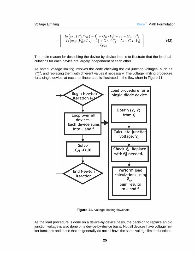
As noted, voltage limiting involves the code checking the old junction voltages, such asV old
12 , and replacing them with different values if necessary. The voltage limiting procedurefor a single device, at each nonlinear step is illustrated in the flow chart in Figure 11.
Figure 11. Voltage limiting flowchart.
As the load procedure is done on a device-by-device basis, the decision to replace an oldjunction voltage is also done on a device-by-device basis. Not all devices have voltage lim-iter functions and those that do generally do not all have the same voltage limiter functions.
25
Xyce TMMath Formulation Nonlinear circuits
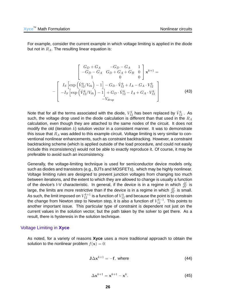
For example, consider the current example in which voltage limiting is applied in the diodebut not in RA. The resulting linear equation is:
GD + GA −GD −GA 1−GD −GA GD + GA + GB 0
1 0 0
xk+1 =
−
IS
[exp
(V k
12/Vth
)− 1
]−GD · V k
12 + IA −GA · V k12
−IS
[exp
(V k
12/Vth
)− 1
]+ GD · V k
12 − IA + GA · V k12
−Vdrop
(43)
Note that for all the terms associated with the diode, V k12 has been replaced by V k
12 . Assuch, the voltage drop used in the diode calculation is different than that used in the RA
calculation, even though they are attached to the same nodes of the circuit. It does notmodify the old (iteration k) solution vector in a consistent manner. It was to demonstratethis issue that RA was added to this example circuit. Voltage limiting is very similar to con-ventional nonlinear enhancements, such as constraint backtracking. However, a constraintbacktracking scheme (which is applied outside of the load procedure, and could not easilyinclude this inconsistency) would not be able to exactly reproduce it. Of course, it may bepreferable to avoid such an inconsistency.
Generally, the voltage-limiting technique is used for semiconductor device models only,such as diodes and transistors (e.g., BJTs and MOSFETs), which may be highly nonlinear.Voltage limiting rules are designed to prevent junction voltages from changing too muchbetween iterations, and the extent to which they are allowed to change is usually a functionof the device’s I-V characteristic. In general, if the device is in a regime in which dI
dV islarge, the limits are more restrictive than if the device is in a regime in which dI
dV is small.As such, the limit imposed on V k+1
12 is a function of V k12 and because the point is to constrain
the change from Newton step to Newton step, it is also a function of V k−112 . This points to
another important issue. This particular type of constraint is dependent not just on thecurrent values in the solution vector, but the path taken by the solver to get there. As aresult, there is hysteresis in the solution technique.
Voltage Limiting in Xyce
As noted, for a variety of reasons Xyce uses a more traditional approach to obtain thesolution to the nonlinear problem f(x) = 0:
J∆xk+1 = −f , where (44)
∆xk+1 = xk+1 − xk. (45)
26
Voltage Limiting Xyce TMMath Formulation
Initially, voltage limiting was not a planned feature for Xyce , in part because the nonlin-ear solver was designed to use the traditional Newton iteration, as described by Equa-tion 44. Once the value of voltage limiting became apparent, it was necessary to reformu-late Spice3f5 implementation to work in Xyce .
For the nonlinear iteration k, the original “unlimited” solution vector is given by xk, theintermediate limited solution vector is given by xk+1, and the final solution vector at theend of the iteration is given by xk+1. Thus, for a Newton step that includes voltage limiting,the total change from the beginning of the step to the end is:
∆xk+1total = ∆xk+1
newton + ∆xk+1 (46)
where:
∆xk+1 = xk+1 − xk (47)
and:
∆xk+1newton = xk+1 − xk+1 (48)
∆xk+1 represents the change in the solution due to voltage limiting, ∆xk+1newton represents
the change due to the solution of the matrix equation, and ∆xk+1total is the total change over
the course of the Newton step. The linear equation to be solved is now:
J∆xk+1total = −f + J∆xk+1 (49)
This equation has been obtained by adding J∆xk+1 to both sides of the original Newtonstep equation.
The calculations performed at each Newton step are very similar using this approach asthey were for the Spice3f5 case. The Xyce version of equation (43) is given by:
J∆xk+1total = −
IS
[exp
(V k+1
12 /Vth
)− 1
]+ IA −GD ·∆V k+1
12
−IS
[exp
(V k+1
12 /Vth
)− 1
]− IA + GD ·∆V k+1
12
Vk+11 − Vdrop
(50)
Or, alternatively:
27
Xyce TMMath Formulation Time Dependent Circuits
J∆xk+1total = −
IS
[exp
(V k+1
12 /Vth
)− 1
]+ IA
−IS
[exp
(V k+1
12 /Vth
)− 1
]− IA
V k+11 − Vdrop
+
GD · V k+112
−GD · V k+112
0
(51)
J∆xk+1total = −
IS
[exp
(V k+1
12 /Vth
)− 1
]+ IA
−IS
[exp
(V k+1
12 /Vth
)− 1
]− IA
V k+11 − Vdrop
+
GD −GD 0−GD GD 0
0 0 0
∆V k+11
∆V k+12
∆Ik+1V src
(52)
One nice feature of this formulation is that as the Newton algorithm approaches conver-gence, the values for ∆xk+1
total become much smaller. By solving for ∆xk+1 rather than xk+1,it is easier to resolve the small changes in the solution that occur during the final iterations.Also, as most nonlinear solver libraries and algorithms are designed for this (∆x) approach,it is much easier to take advantage of them. Finally, the final (J∆xk+1) term on the righthand side of equation (52) can easily be stored in a separate vector than the first (−f ) term,so algorithms depending upon f are impacted less than in the other case.
Additional Notes
Xyce has a large number of different nonlinear solver options, including damped Newton,modified Newton, inexact-Newton, constraint backtracking, and gradient-based methods.A complete list of options, and a guide to usage is contained in [8]. In general, mostnonlinear solver strategies are incompatible with voltage limiting, either because of theunorthodox right hand side vector, or because of the hysteresis introduced by the limiters.Some future work may include finding ways to combine the effect of the limiters with someof the other methods. The voltage limiter technique has been one of the most effectivetechniques, especially for semiconductor circuits.
5 Time Dependent CircuitsIn practice, most circuits contain a number of time dependent elements, and many ofthose elements (capacitors and inductors) are described by ordinary differential equations(ODEs) that include time derivative terms. For example, the current in a linear capacitor isgiven by:
IC =dq
dt(53)
28
Traditional Index-1 DAE Formulation for the Linear Case Xyce TMMath Formulation
Capacitors are particularly ubiquitous, as not only are they usually present as distinct de-vices, but they also appear as subcomponents in every semiconductor device model. Whilethe inclusion of such devices requires that the mathematical formulation include ODEs, theoverall formulation is still based upon modified nodal analysis, and as such, the set ofequations to be solved contains a number of purely algebraic equations. These includethe voltage drop equation for a voltage source, or any KCL equation that includes only re-sistor currents. The set of equations, therefore, is a set of differential-algebraic equations(DAEs), where those that are purely algebraic are considered to be the constraints.
There is a lot of literature devoted to describing DAEs and methods for their solution [5, 4].For the most part, that material will not be described here as it is beyond the scope ofthis document. Most systems of equations resulting from circuit theory can be cast asDAEs of index one, and fortunately the techniques for solving DAEs of index one are fairlywell understood. It is possible, particularly in circuits containing operational amplifiers, toobtain DAEs of much higher index [5], but at the moment such circuits are not possibleto simulate in Xyce , so they will not be considered here. Xyce and Spice3f5 both use acondensed form of the circuit equations that will be described in the third subsection of thissection. This condensed form appears to be a standard technique for circuit simulation,and has some obvious advantages, but for the most part this condensed form has notbeen described in the literature. In practice, it appears to work reasonably well, but thenumerical implications (stability, accuracy, etc.) of using such a form are not entirely clearat this point.
5.1 Traditional Index-1 DAE Formulation for the LinearCase
Differential Algebraic Equations (DAEs) generally have the form:
f(x,
dxdt
, t
)= 0 (54)
For the linear case, this is often presented in the form of a matrix equation:
f = Ax + Bdxdt
+ r(t) = 0 (55)
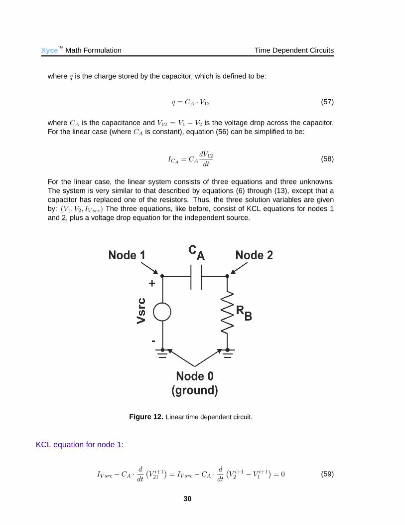
In equation (55), A and B are matrices and r(t) is a source term. This formalism caneasily be applied to the linear circuit that is presented in Figure 12. This circuit is the sameas all of the previous example circuits, except that now a capacitor sits between nodes 1and 2. The capacitor, CA, is a time dependent device, and has a current defined to be:
ICA=
dq
dt(56)
29
Xyce TMMath Formulation Time Dependent Circuits
where q is the charge stored by the capacitor, which is defined to be:
q = CA · V12 (57)
where CA is the capacitance and V12 = V1 − V2 is the voltage drop across the capacitor.For the linear case (where CA is constant), equation (56) can be simplified to be:
ICA= CA
dV12
dt(58)
For the linear case, the linear system consists of three equations and three unknowns.The system is very similar to that described by equations (6) through (13), except that acapacitor has replaced one of the resistors. Thus, the three solution variables are givenby: (V1, V2, IV src) The three equations, like before, consist of KCL equations for nodes 1and 2, plus a voltage drop equation for the independent source.
Figure 12. Linear time dependent circuit.
KCL equation for node 1:
IV src − CA ·d
dt
(V i+1
21
)= IV src − CA ·
d
dt
(V i+1
2 − V i+11
)= 0 (59)
30
Traditional Index-1 DAE Formulation for the Linear Case Xyce TMMath Formulation
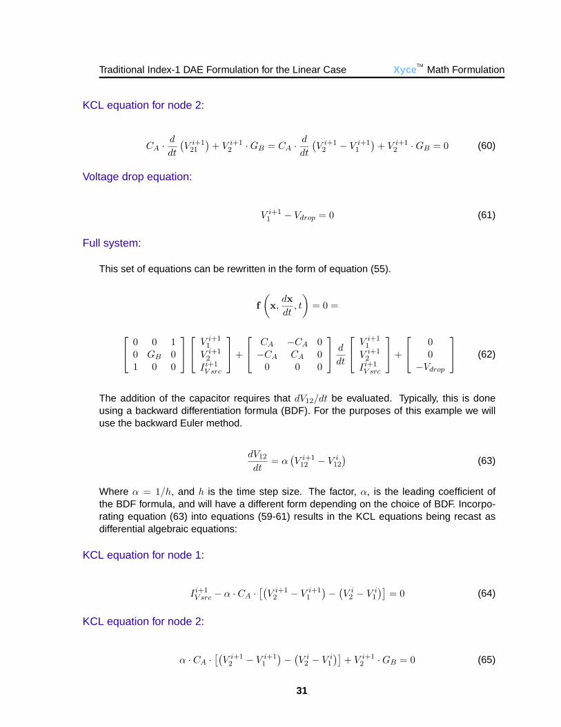
KCL equation for node 2:
CA ·d
dt
(V i+1
21
)+ V i+1
2 ·GB = CA ·d
dt
(V i+1
2 − V i+11
)+ V i+1
2 ·GB = 0 (60)
Voltage drop equation:
V i+11 − Vdrop = 0 (61)
Full system:
This set of equations can be rewritten in the form of equation (55).
f(x,
dxdt
, t
)= 0 =
0 0 10 GB 01 0 0
V i+11
V i+12
Ii+1V src
+
CA −CA 0−CA CA 0
0 0 0
d
dt
V i+11
V i+12
Ii+1V src
+
00
−Vdrop
(62)
The addition of the capacitor requires that dV12/dt be evaluated. Typically, this is doneusing a backward differentiation formula (BDF). For the purposes of this example we willuse the backward Euler method.
dV12
dt= α
(V i+1
12 − V i12
)(63)
Where α = 1/h, and h is the time step size. The factor, α, is the leading coefficient ofthe BDF formula, and will have a different form depending on the choice of BDF. Incorpo-rating equation (63) into equations (59-61) results in the KCL equations being recast asdifferential algebraic equations:
KCL equation for node 1:
Ii+1V src − α · CA ·
[(V i+1
2 − V i+11
)−
(V i
2 − V i1
)]= 0 (64)
KCL equation for node 2:
α · CA ·[(
V i+12 − V i+1
1
)−
(V i
2 − V i1
)]+ V i+1
2 ·GB = 0 (65)
31
Xyce TMMath Formulation Time Dependent Circuits
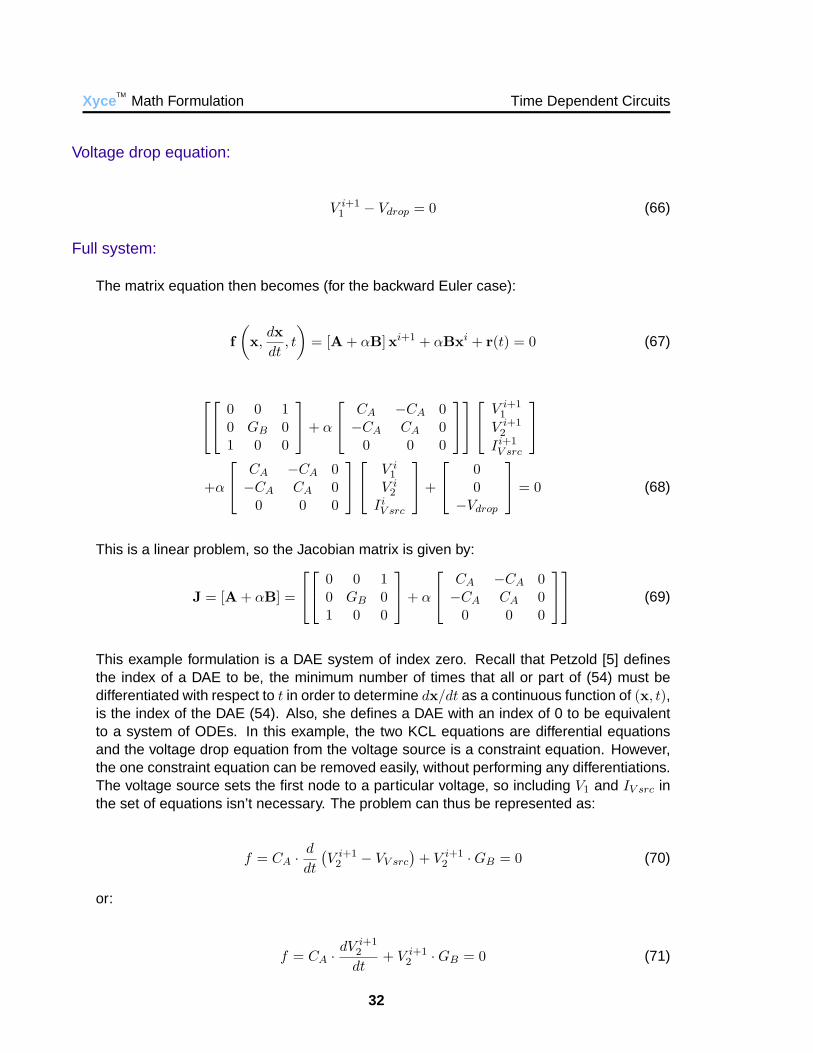
Voltage drop equation:
V i+11 − Vdrop = 0 (66)
Full system:
The matrix equation then becomes (for the backward Euler case):
f(x,
dxdt
, t
)= [A + αB]xi+1 + αBxi + r(t) = 0 (67)
0 0 10 GB 01 0 0
+ α
CA −CA 0−CA CA 0
0 0 0
V i+11
V i+12
Ii+1V src
+α
CA −CA 0−CA CA 0
0 0 0
V i1
V i2
IiV src
+
00
−Vdrop
= 0 (68)
This is a linear problem, so the Jacobian matrix is given by:
J = [A + αB] =
0 0 10 GB 01 0 0
+ α
CA −CA 0−CA CA 0
0 0 0
(69)
This example formulation is a DAE system of index zero. Recall that Petzold [5] definesthe index of a DAE to be, the minimum number of times that all or part of (54) must bedifferentiated with respect to t in order to determine dx/dt as a continuous function of (x, t),is the index of the DAE (54). Also, she defines a DAE with an index of 0 to be equivalentto a system of ODEs. In this example, the two KCL equations are differential equationsand the voltage drop equation from the voltage source is a constraint equation. However,the one constraint equation can be removed easily, without performing any differentiations.The voltage source sets the first node to a particular voltage, so including V1 and IV src inthe set of equations isn’t necessary. The problem can thus be represented as:
f = CA ·d
dt
(V i+1
2 − VV src
)+ V i+1
2 ·GB = 0 (70)
or:
f = CA ·dV i+1
2
dt+ V i+1
2 ·GB = 0 (71)
32
Traditional Index-1 DAE Formulation for the Nonlinear Case Xyce TMMath Formulation
Equation (71) is a single implicit ODE. This conversion to an ODE, which removes thealgebraic constraints, results in the need for an initial condition on V2. It should be notedthat most circuit problems do not result in a DAE of index zero. Instead, the systems aretypically of index one, and some examples of higher index systems will be given in followingsections. For linear circuits, the DAE formulation just described (before the removal of thevoltage source equation) matches that of Xyce . In the next section, the most obvious wayof handling the nonlinear case will be addressed.
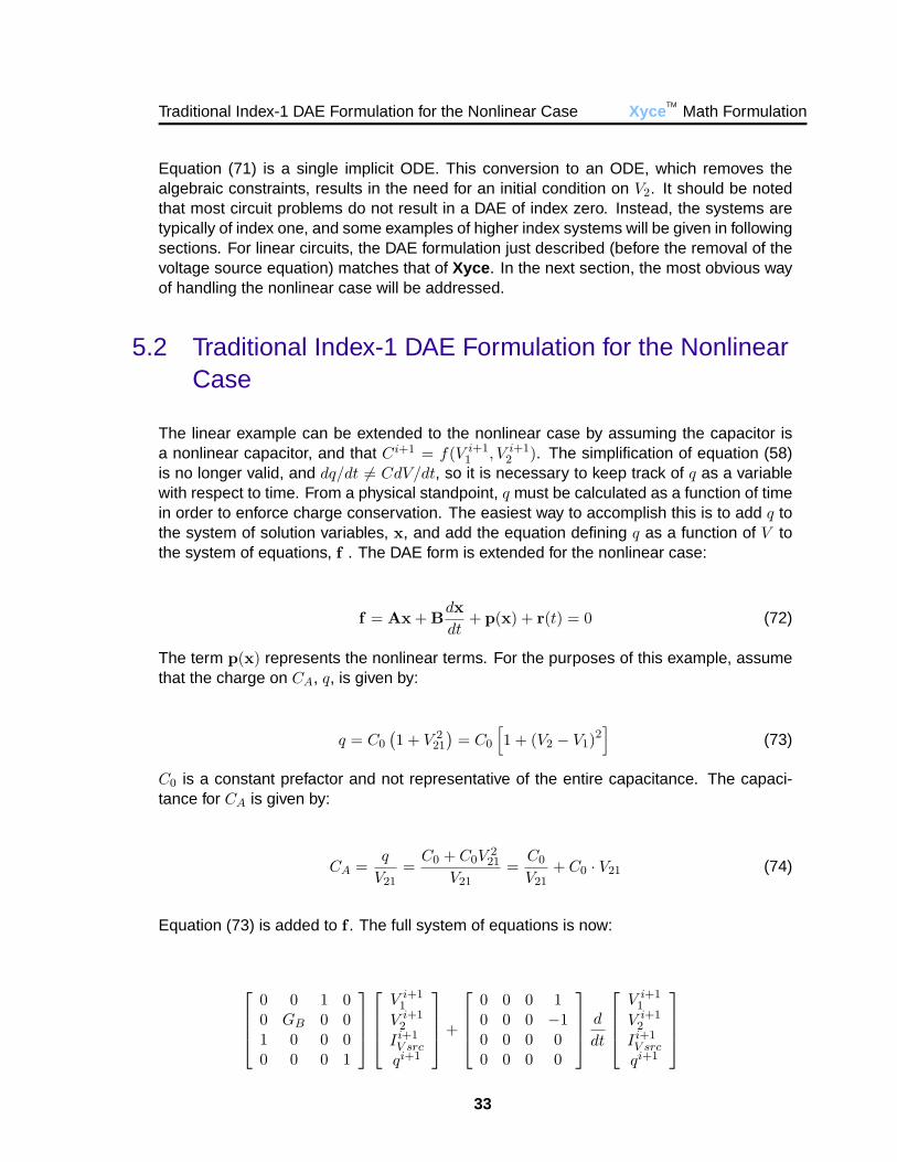
5.2 Traditional Index-1 DAE Formulation for the NonlinearCase
The linear example can be extended to the nonlinear case by assuming the capacitor isa nonlinear capacitor, and that Ci+1 = f(V i+1
1 , V i+12 ). The simplification of equation (58)
is no longer valid, and dq/dt 6= CdV/dt, so it is necessary to keep track of q as a variablewith respect to time. From a physical standpoint, q must be calculated as a function of timein order to enforce charge conservation. The easiest way to accomplish this is to add q tothe system of solution variables, x, and add the equation defining q as a function of V tothe system of equations, f . The DAE form is extended for the nonlinear case:
f = Ax + Bdxdt
+ p(x) + r(t) = 0 (72)
The term p(x) represents the nonlinear terms. For the purposes of this example, assumethat the charge on CA, q, is given by:
q = C0
(1 + V 2
21
)= C0
[1 + (V2 − V1)
2]
(73)
C0 is a constant prefactor and not representative of the entire capacitance. The capaci-tance for CA is given by:
CA =q
V21=
C0 + C0V221
V21=
C0
V21+ C0 · V21 (74)
Equation (73) is added to f . The full system of equations is now:
0 0 1 00 GB 0 01 0 0 00 0 0 1
V i+11
V i+12
Ii+1V src
qi+1
+
0 0 0 10 0 0 −10 0 0 00 0 0 0
d
dt
V i+1
1
V i+12
Ii+1V src
qi+1
33
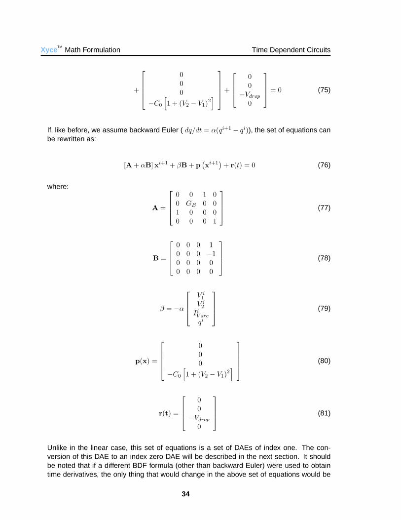
Xyce TMMath Formulation Time Dependent Circuits
+
000
−C0
[1 + (V2 − V1)
2]
+
00
−Vdrop
0
= 0 (75)
If, like before, we assume backward Euler ( dq/dt = α(qi+1 − qi)), the set of equations canbe rewritten as:
[A + αB]xi+1 + βB + p(xi+1
)+ r(t) = 0 (76)
where:
A =
0 0 1 00 GB 0 01 0 0 00 0 0 1
(77)
B =
0 0 0 10 0 0 −10 0 0 00 0 0 0
(78)
β = −α
V i
1
V i2
IiV src
qi
(79)
p(x) =
000
−C0
[1 + (V2 − V1)
2]
(80)
r(t) =
00
−Vdrop
0
(81)
Unlike in the linear case, this set of equations is a set of DAEs of index one. The con-version of this DAE to an index zero DAE will be described in the next section. It shouldbe noted that if a different BDF formula (other than backward Euler) were used to obtaintime derivatives, the only thing that would change in the above set of equations would be
34
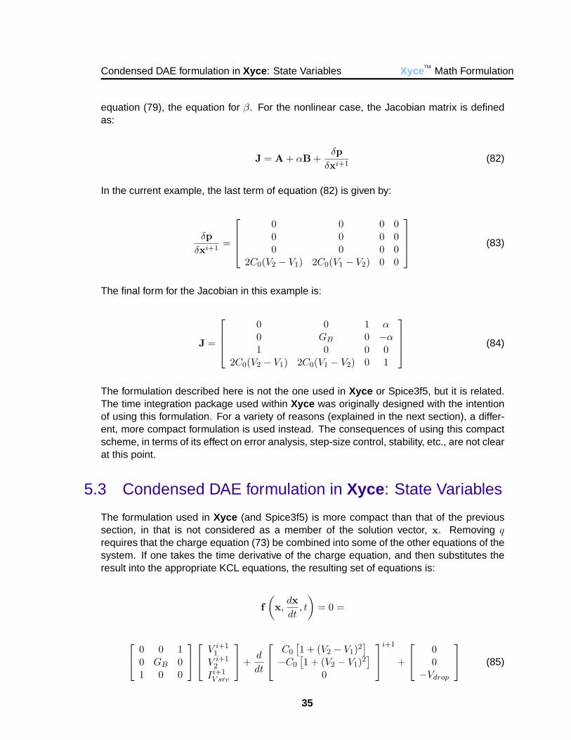
Condensed DAE formulation in Xyce : State Variables Xyce TMMath Formulation
equation (79), the equation for β. For the nonlinear case, the Jacobian matrix is definedas:
J = A + αB +δp
δxi+1(82)
In the current example, the last term of equation (82) is given by:
δpδxi+1
=
0 0 0 00 0 0 00 0 0 0
2C0(V2 − V1) 2C0(V1 − V2) 0 0
(83)
The final form for the Jacobian in this example is:
J =
0 0 1 α0 GB 0 −α1 0 0 0
2C0(V2 − V1) 2C0(V1 − V2) 0 1
(84)
The formulation described here is not the one used in Xyce or Spice3f5, but it is related.The time integration package used within Xyce was originally designed with the intentionof using this formulation. For a variety of reasons (explained in the next section), a differ-ent, more compact formulation is used instead. The consequences of using this compactscheme, in terms of its effect on error analysis, step-size control, stability, etc., are not clearat this point.
5.3 Condensed DAE formulation in Xyce : State Variables
The formulation used in Xyce (and Spice3f5) is more compact than that of the previoussection, in that is not considered as a member of the solution vector, x. Removing qrequires that the charge equation (73) be combined into some of the other equations of thesystem. If one takes the time derivative of the charge equation, and then substitutes theresult into the appropriate KCL equations, the resulting set of equations is:
f(x,
dxdt
, t
)= 0 =
0 0 10 GB 01 0 0
V i+11
V i+12
Ii+1V src
+d
dt
C0
[1 + (V2 − V1)2
]−C0
[1 + (V2 − V1)2
]0
i+1
+
00
−Vdrop
(85)
35
Xyce TMMath Formulation Time Dependent Circuits
This procedure appears to have the effect of reducing the index from one to zero, becausenow equation (85) is in a similar form to that of equation (62) before the application of theBDF. It is still a DAE, however, and not an ODE system. To reduce it further to an ODEsystem, one should follow the same procedure as outlined in equations (70) and (71), andremove the constraint equation for the voltage source.
Generally the lower the index of a DAE, the easier it is to solve, although there can beunintended consequences. Another (perhaps more important) benefit of this condensationis that the size of the linear system has been reduced. As will be explained later, this typeof equation elimination results in a very significant problem size reduction for most largecircuits. This reduction bears some similarity to the derivation of the pressure-Poissonequation in fluid mechanics [4], and the use of the range-space method in constrainedoptimization problems [11] . In the case of circuit equations, this reduction does not removeall the constraint equations of the system, so the set of equations is still a set of DAEs, butwith index zero.
One issue of interest is that now the variables that are part of the solution vector, x, areno longer the same as the variables for which we need time derivatives. In this particularexample, we need the time derivative of the capacitor charge, q, but we do not need timederivatives for V1, V2 or IV src. In this document, variables that are part of x will be referredto as solution variables, while variables that are not part of x but are needed by the timeintegration algorithm will be referred to as “state variables”.
This choice of naming convention is consistent with that of the data structures in Spice3f5,but it has the potential to cause confusion. The term, state variable, is often used asthe equivalent of the term, solution variable, in much of the circuit simulation literature[9, 7], and other contexts. Additionally, there exists a mathematical formulation of thecircuit equations known as the “state variable formulation”, in which the circuit equationsare an implicit ODE system. Chua and Lin describe this formulation in detail [6]. Thisformulation is not commonly used in modern circuit simulators, as it has been proven thatsome circuits cannot be represented in this form.
The inexact Jacobian used with the condensed form
The condensed form described in the previous section has been implemented with onetype of approximation made in the calculation of the Jacobian matrix. There is nothingabout the condensed form that requires the use of this approximation, but it facilitates theimplementation. This approximation is made in Spice3f5 and Xyce for the Jacobian matrixcontributions associated with a nonlinear capacitor. The two-terminal nonlinear capacitorcontributes the following stencil to the linear system:
36
Condensed DAE formulation in Xyce : State Variables Xyce TMMath Formulation
......
. . . δIC/δV1 . . . δIC/δV2 . . ....
.... . . −δIC/δV1 . . . −δIC/δV2 . . .
......
...∆V1
...∆V2
...
= −
...IC...
−IC...
(86)
Generally, δIC/δV1 = −δIC/δV2, so all the terms in the Jacobian stencil are of the samemagnitude. Recall that the capacitor current is given by:
IC =dq
dt(87)
For the linear capacitor, this can be simplified to:
IC =dV12
dt(88)
Time derivatives are approximated, in general using a BDF:
dV i+1
dt= αV i+1 + βV i + γV i−1 + . . . (89)
For the purposes of calculating the Jacobian terms, only the leading term of the BDF isneeded, as the partial derivatives used in the matrix are all in terms if new (i+1) variables.So, for the linear capacitor, the form of the Jacobian term is:
δI
δV= αC (90)
For the nonlinear capacitor, C is dependent upon the capacitor voltage at i + 1, so forthat case, equation (90) is not correct. However, in Spice3f5 and Xyce it is often (but notalways) used anyway. For nonlinear problems it is often not necessary that the Jacobianbe perfect, and that appears to be the case for circuit problems. However, this may turnout to be inadequate for optimization studies in the future [11] . It is not necessary to usethis approximation in the compact state variable formulation, but implementation is easier,as it is not necessary to calculate the partial derivative of C with respect to V . Also, allcapacitors types, both linear and nonlinear, are now handled in the same way.
Reduction in Jacobian size resulting form the condensed form
The impact of using the condensed formulation is significant enough that real life circuitcodes (such as commercial implementations of SPICE [1], and non-SPICE circuit codes
37
Xyce TMMath Formulation Time Dependent Circuits
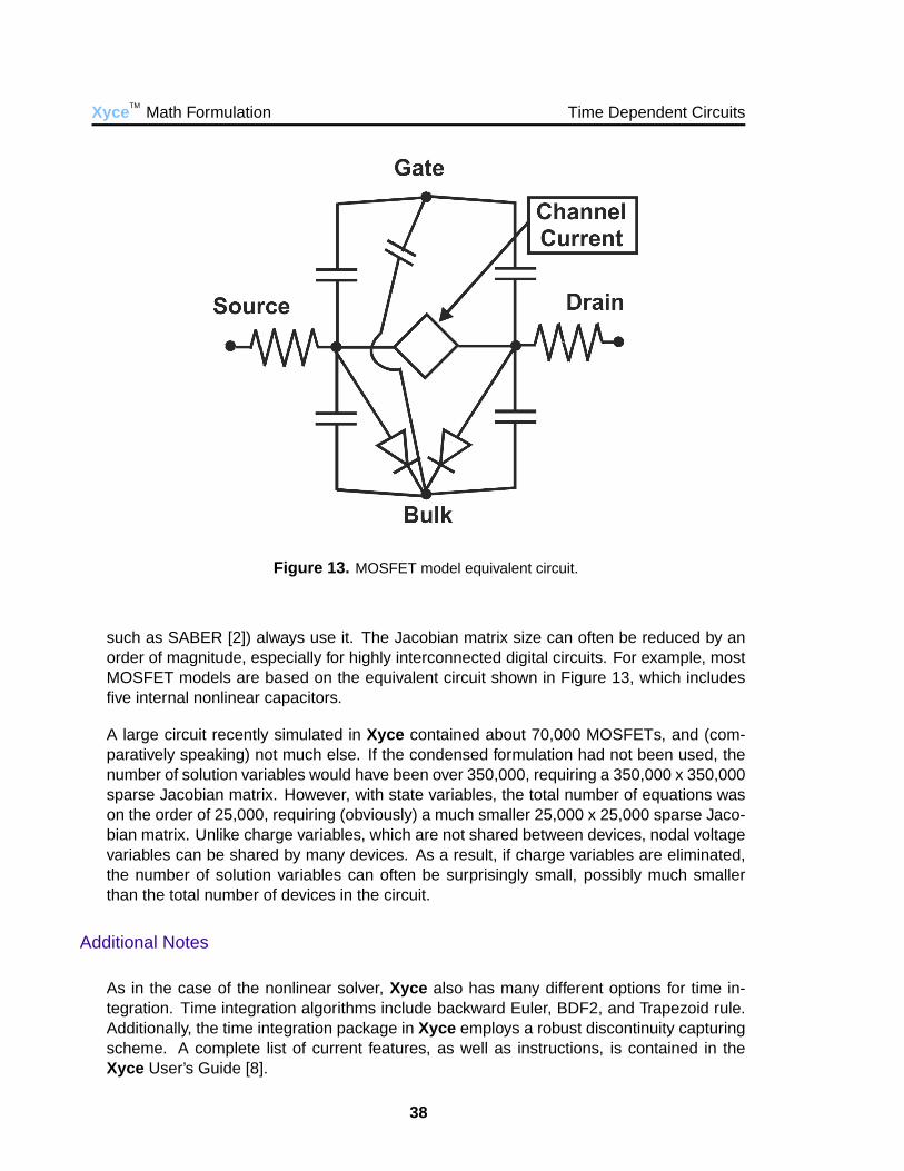
Figure 13. MOSFET model equivalent circuit.
such as SABER [2]) always use it. The Jacobian matrix size can often be reduced by anorder of magnitude, especially for highly interconnected digital circuits. For example, mostMOSFET models are based on the equivalent circuit shown in Figure 13, which includesfive internal nonlinear capacitors.
A large circuit recently simulated in Xyce contained about 70,000 MOSFETs, and (com-paratively speaking) not much else. If the condensed formulation had not been used, thenumber of solution variables would have been over 350,000, requiring a 350,000 x 350,000sparse Jacobian matrix. However, with state variables, the total number of equations wason the order of 25,000, requiring (obviously) a much smaller 25,000 x 25,000 sparse Jaco-bian matrix. Unlike charge variables, which are not shared between devices, nodal voltagevariables can be shared by many devices. As a result, if charge variables are eliminated,the number of solution variables can often be surprisingly small, possibly much smallerthan the total number of devices in the circuit.
Additional Notes
As in the case of the nonlinear solver, Xyce also has many different options for time in-tegration. Time integration algorithms include backward Euler, BDF2, and Trapezoid rule.Additionally, the time integration package in Xyce employs a robust discontinuity capturingscheme. A complete list of current features, as well as instructions, is contained in theXyce User’s Guide [8].
38

Condensed DAE formulation in Xyce : State Variables Xyce TMMath Formulation
It should be noted that currently, the only option in Xyce is the condensed DAE form.The option for using the non-condensed traditional formulation, presented in the previoussection, is not currently available (Xyce Release 2.0). As of this writing, the Xyce timeintegrator is in the process of being redesigned, so other formulations may be available inthe future.
39
Xyce TMMath Formulation REFERENCES
References[1] Hspice user’s manual. Technical report, Meta-Software, Inc., Campbell, California,
1996.
[2] Saber mixed signal simulator user’s manual. Technical report, Analogy Software,Beaverton, Oregon, 2001.
[3] NOX and LOCA:Object-Oriented Nonlinear Solver and Continuation Packages.http://software.sandia.gov/nox/, 2004.
[4] Uri M. Ascher and Linda R. Petzold. Computer Methods for Ordinary DifferentialEquations and Differential-Algebraic Equations. SIAM, Philadelphia, 1988.
[5] K. E. Brenen S. L. Campbell and L. R. Petzold. Numerical Solution of Initial-ValueProblems in Differential-Algebraic Equations. Prentice-Hall, North-Holland, New York,1989.
[6] Leon O. Chua and Pen-Min Lin. Computer-Aided Analysis of Electronic Circuits: Algo-rithms and Computational Techniques. Prentice-Hall, Englewood Cliffs, New Jersey,1975.
[7] Daniel Foty. MOSFET Modeling with SPICE. Principles and Practice. Prentice-Hall,Upper Saddle River, New Jersey, 1997.
[8] Scott A. Hutchinson, Eric R. Keiter, Robert J. Hoekstra, Lon J. Waters, Thomas V.Russo, Eric L. Rankin, Roger P. Pawlowski, and Steven D. Wix. Xyce parallel elec-tronic simulator: User’s guide, version 2.0. Technical Report SAND2003-xxxx, SandiaNational Laboratories, Albuquerque, NM, December 2003.
[9] William Liu. MOSFET Models for SPICE Simulation including BSIM3v3 and BSIM4.John Wiley and Sons, New York, 2001.
[10] Laurence Nagel and Ronald Rohrer. Computer analysis of nonlinear circuits, exclud-ing radiation (cancer). IEEE Journal of Solid-State Circuits, sc-6(4):166–182, 1971.
[11] Jorge Nocedal and Stephen J. Wright. Numerical Optimization. Springer-Verlag, NewYork, 1999.
[12] C. W. Ho A. E. Ruehli and P. A. Brennan. The modified nodal approach to networkanalysis. IEEE Trans. Circuits Systems, 22:505–509, 1988.
[13] Gilbert Strang. A framework for equilibrium equations. SIAM Review, 30(2):283–297,June 1988.
[14] Jiri Vlach and Kishore Singal. Computer Methods for Circuit Analysis and Design.Chapman and Hall, New York, 1994.
40
IndexBJT, 26
Capacitor, 29
DAE, 29Index, 32
Linear Index-1 Circuit problem, 29Nonlinear Index-1 Circuit problem,
33Diode, 17Diode equation, 17
Kirchhoff’s Laws, 10KCL - Kirchhoff’s Current Law, 10KVL - Kirchhoff’s Voltage Law, 10
Modifed KCL Formualtion, 12Modified Nodal Analysis (MNA), 12MOSFET, 26, 37
Nonlinear circuits, 17
ODE, 28Ohm’s Law, 12
Resistor, 12
Spice3f5, 12, 20–24, 27, 29, 35–37Voltage Limiting, 21
State Variables, 35Inexact Jacobian, 36
Tableau Formulation, 11Time Dependent Circuits, 28
Voltage Limiting, 20in Xyce , 26in Spice3f5, 21
Voltage Source, 13
41
Xyce TMMath Formulation INDEX
DISTRIBUTION:
1 Steven P. CastilloKlipsch School of Electrical andComputer EngineeringNew Mexico State UniversityBox 3-oLas Cruces, NM 88003
1 Kwong T. NgKlipsch School of Electrical andComputer EngineeringNew Mexico State UniversityBox 3-oLas Cruces, NM 88003
1 Nick HitchonElectrical and Computer Engi-neeringUniversity of Wisconsin1415 Engineering DriveMadison, WI 53706
1 Mark KushnerDepartment of Electrical andComputer EngineeringUniversity of Illinois1406 W. Green StreetUrbana, IL 61801
1 Ron KielkowskiRCG Research, Inc8605 Allisonville Rd, Suite 370Indianapolis, In 46250
1 Mike DavisSoftware Federation, Inc.211 Highview DriveBoulder, Co 80304
1 Wendland BeezholdIdaho Accelerator Center1500 Alvin Ricken DrivePocatello, Idaho 83201
1 Kartikeya MayaramDepartment of Electrical andComputer EngineeringOregon State UniversityCorvallis, OR 97331-3211
1 Linda PetzoldDepartment of Computer Sci-enceUniversity of California, SantaBarbaraSanta Barbara, CA 93106-5070
1 Jaijeet Roychowdhury4-174 EE/CSci Building200 Union Street S.E.University of MinnesotaMinneapolis, MN 55455
1 C.-J. Richard ShiVLSI and Electronic Design Au-tomation210 EE/CSE Bldg.Box 352500University of WashingtonSeattle, WA 98195
1 Homer F. WalkerWPI Mathematical Sciences100 Institute RoadWorcester, MA 01609
1 Dan YergeauCISX 334Via OrtegaStanford, CA 94305-4075
1 Masha Sosonkina319 Heller Hall10 University Dr.Duluth, MN 55812
1 Misha Elena Kilmer113 Bromfield-Pearson Bldg.Tufts UniversityMedford, MA 02155
1 Tim DavisP.O. Box 116120University of FloridaGainesville, FL 32611-6120
42
INDEX Xyce TMMath Formulation
1 Achim BasermannC&C Research Laboratories,NEC Europe Ltd.Rathausallee 10D-53757 Sankt AugustinGermany
1 Philip A. WilseyClifton Labs7450 Montgomery RoadSuite 300Cincinnati, Ohio 45236
1 Dale E. MartinClifton Labs7450 Montgomery RoadSuite 300Cincinnati, Ohio 45236
1 Richard L. KeiterDepartment of ChemistryEastern Illinois University600 Lincoln AvenueCharleston, IL 61920
1 Ellen A. KeiterDepartment of ChemistryEastern Illinois University600 Lincoln AvenueCharleston, IL 61920
1 Lise Keiter-Brotzman10 College CircleStaunton, VA 24401
1 Al LehnenMathematics DepartmentMadison Area Technical Col-lege3550 Anderson StreetMadison, WI 53704
1 Lon WatersCoMet Solutions, Inc.11811 Menaul Blvd NESuite No. 1Albuquerque, NM 87112
1 Tim DavisP.O. Box 116120University of FloridaGainesville, FL 32611-6120
1 MS 0321Bill Camp, 09200
1 MS 0318Paul Yarrington, 09230
1 MS 1071Mike Knoll, 01730
1 MS 0310Robert Leland, 09220
1 MS 0316Sudip Dosanjh, 09233
1 MS 0525Paul V. Plunkett, 01734
1 MS 0835J. Michael McGlaun, 09140
1 MS 0828Anthony A. Giunta, 09133
1 MS 0139Stephen E. Lott, 09905
1 MS 0310Mark D. Rintoul, 09212
1 MS 1110David Womble, 09214
1 MS 1111Bruce Hendrickson, 09215
1 MS 0819Edward Boucheron, 09231
1 MS 0819Allen C. Robinson, 09231
1 MS 0316John Aidun, 09235
1 MS 0316Scott A. Hutchinson, 09233
43
Xyce TMMath Formulation INDEX
10 MS 0316Eric R. Keiter, 09233
1 MS 0316Deborah Fixel, 09233
1 MS 0316Robert J. Hoekstra, 09233
1 MS 0316Brett Bader, 09233
1 MS 0316Joseph P. Castro, 09233
1 MS 0316David R. Gardner, 09233
1 MS 0316Gary Hennigan, 09233
1 MS 0316Eric Phipps, 09233
1 MS 0316Eric L. Rankin, 09233
1 MS 0316Roger Pawlowski, 09233
1 MS 0316Richard Schiek, 09233
1 MS 1111John N. Shadid, 09233
1 MS 1111Andrew Salinger, 09233
1 MS 0316Paul Lin, 09233
1 MS 0316Siriphone C. Kuthakun, 09233
1 MS 0807David N. Shirley, 9328
1 MS 0807Philip M. Campbell, 9328
1 MS 0847Scott Mitchell, 09211
1 MS 0847Mike Eldred, 09211
1 MS 0847Bart van Bloemen Waanders,09211
1 MS 0847Roscoe A. Bartlett, 09211
1 MS 0196Elebeoba May, 09212
1 MS 1110Todd Coffey, 09214
1 MS 1110David Day, 09214
1 MS 1110Mike Heroux, 09214
1 MS 1110Pavel B. Bochev, 09214
1 MS 1110Richard B. Lehoucq, 09214
1 MS 1110Raymond S. Tuminaro, 09214
1 MS 1110James Willenbring, 09214
1 MS 1111Karen Devine, 09215
1 MS 1109Robert Benner, 09224
1 MS 0316Harry Hjalmarson, 09235
1 MS 0525Steven D. Wix, 01734
1 MS 0525Thomas V. Russo, 01734
44
INDEX Xyce TMMath Formulation
1 MS 0525Regina Schells, 01734
1 MS 0525Carolyn Bogdan, 01734
1 MS 0525Mike Deveney, 01734
1 MS 0525Raymond B. Heath, 01734
1 MS 0525Ronald Sikorksi, 01734
1 MS 0525Albert Nunez, 01734
1 MS 1081Paul E. Dodd, 01762
1 MS 0660Roger F. Billau, 09519
1 MS 0874Robert Brocato, 01751
1 MS 1081Charles E. Hembree, 01739
1 MS 0889Neil R. Sorenson, 01832
1 MS 0311Greg Lyons, 02616
1 MS 0311Martin Stevenson, 02616
1 MS 0328Fred Anderson, 02612
1 MS 0537Perry Molley, 02331
1 MS 0537Siviengxay Limary, 02331
1 MS 0537John Dye, 02331
1 MS 0537Barbara Wampler, 02331
1 MS 0537Doug Weiss, 02333
1 MS 0537Scott Holswade, 02333
1 MS 0537George R. Laguna, 02333
1 MS 0481Joel Brown, 02132
1 MS 0405Todd R. Jones, 12333
1 MS 0405Thomas D. Brown, 12333
1 MS 0405Donald C. Evans, 12333
1 MS 0405Matthew T. Kerschen, 12333
1 MS 9101Rex Eastin, 08232
1 MS 9101Seung Choi, 08235
1 MS 9409William P. Ballard, 08730
1 MS 9202Kathryn R. Hughes, 08205
1 MS 9202Rene L. Bierbaum, 08205
1 MS 9202Kenneth D. Marx, 08205
1 MS 9202Stephen L. Brandon, 08205
1 MS 9202Jason Dimkoff, 08205
1 MS 9202Brian E. Owens, 08205
45
Xyce TMMath Formulation INDEX
1 MS 9401Donna J. O’Connell, 08751
1 MS 9217Stephen W. Thomas, 08950
1 MS 9217Tamara G. Kolda, 08950
1 MS 9217Kevin R. Long, 08950
1 MS 9915Mitchel W. Sukalski, 08961
1 MS 1153Larry D. Bacon, 15333
1 MS 1179Leonard Lorence, 15341
1 MS 1179David E. Beutler, 15341
1 MS 1179Brian Franke, 15341
1 MS 0835Randy Lorber, 09141
1 MS 1152Mark L. Kiefer, 01642
1 MS 1137Greg D. Valdez, 06224
1 MS 1137Mark A. Gonzales, 06224
1 MS 1138Rebecca Arnold, 06223
1 MS 1138Charles Michael Williamson,06223
1 MS 1138Harvey C. Ogden, 06223
1 MS 9018Central Technical Files,8945-1
2 MS 0899Technical Library, 9616
1 MS 0612Review & Approval Desk, forDOE/OSTI, 9612
46