Mathematical Modeling of Electrocardiograms: A … · Mathematical Modeling of Electrocardiograms: A Numerical ... ECG simulator can also be useful in building a ... Mathematical

Mathematical Modeling of Electrocardiograms: A Numerical Study

MURIEL BOULAKIA,1 SERGE CAZEAU,2 MIGUEL A. FERNANDEZ,3 JEAN-FREDERIC GERBEAU,3

and NEJIB ZEMZEMI3,4

1Laboratoire Jacques-Louis Lions, Universite Pierre et Marie Curie-Paris 6, UMR 7598, 75005 Paris, France; 2Departement deRythmologie-Stimulation, Hopital Saint-Joseph, 185, rue Raymond Losserand, 75014 Paris, France; 3INRIA, CRI Paris-Rocquencourt, Rocquencourt BP 105, 78153 Le Chesnay Cedex, France; and 4Laboratoire de mathematiques d’Orsay,

Universite Paris 11, Batiment 425, 91405 Orsay Cedex, France

(Received 30 June 2009; accepted 9 December 2009)

Associate Editor Kenneth R. Lutchen oversaw the review of this article.

Abstract—This paper deals with the numerical simulation ofelectrocardiograms (ECG). Our aim is to devise a mathe-matical model, based on partial differential equations, whichis able to provide realistic 12-lead ECGs. The main ingredi-ents of this model are classical: the bidomain equationscoupled to a phenomenological ionic model in the heart, anda generalized Laplace equation in the torso. The obtention ofrealistic ECGs relies on other important features—includingheart–torso transmission conditions, anisotropy, cell hetero-geneity and His bundle modeling—that are discussed indetail. The numerical implementation is based on state-of-the-art numerical methods: domain decomposition tech-niques and second order semi-implicit time marchingschemes, offering a good compromise between accuracy,stability and efficiency. The numerical ECGs obtained withthis approach show correct amplitudes, shapes and polarities,in all the 12 standard leads. The relevance of every modelingchoice is carefully discussed and the numerical ECG sensi-tivity to the model parameters investigated.

Keywords—12-Lead electrocardiogram, Mathematical mod-

eling, Numerical simulation, Bidomain equation, Ionic

model, Heart–torso coupling, Monodomain equation, Sen-

sitivity analysis.

INTRODUCTION

The electrocardiogram (ECG) is a noninvasiverecording of the electrical activity of the heart,obtained from a standard set of skin electrodes andpresented to the physician as the ‘‘12-lead ECG’’: i.e.,12 graphs of the recorded voltage vs. time. The ECGcan be considered as the most widely used clinical toolfor the detection and diagnosis of a broad range ofcardiac conditions (see e.g. Aehlert,1 Goldberger24).

Despite that, the clinical significance of some ECGfindings is still not fully understood. Computer basedsimulations of the ECG, linking models of the electri-cal activity of the heart (in normal or pathologicalcondition) to the ECG signal, can therefore be avaluable tool for improving this knowledge. Such anECG simulator can also be useful in building a virtualdata base of pathological conditions, in order to testand train medical devices.16 Moreover, being able tosimulate realistic ECGs is a necessary step toward thedevelopment of patient-specific models from clinicalECG data.

The mathematical modeling of the ECG is known asthe forward problem of electrocardiography.32 It relieson three main ingredients: a model for the electricalactivity of the heart, a model for the torso (extracar-diac regions) and some specific heart–torso couplingconditions. Within each of these components, severaloptions are possible, with different levels of complexityand realism (see Lines et al.32 for a recent compre-hensive review).

Although many works have been devoted to thenumerical simulation of cardiac electrophysiology (seee.g. the monographs44,47,51 and the references therein),only a small number28,30,32,41,43,54 addresses thenumerical simulation of ECGs using a whole-heartreaction-diffusion (i.e. bidomain or monodomain)model. Among them, only a very few41,43 providemeaningful simulations of the complete 12-lead ECG.These simulations rely on a monodomain description ofthe electrical activity of the heart, a decoupling of theheart and the torso (isolated heart assumption) and amulti-dipole approximation of the cardiac source withinthe torso (see Sect. 4.2.4 in Lines et al.,32 and Gulra-jani26). To the best of our knowledge, none of theexisting approaches based on partial differential equa-tions (PDE) anda fully coupled heart–torso formulation

Address correspondence to Miguel A. Fernandez, INRIA, CRI

Paris-Rocquencourt, Rocquencourt BP 105, 78153 Le Chesnay

Cedex, France. Electronic mail: [email protected]

Annals of Biomedical Engineering (� 2009)

DOI: 10.1007/s10439-009-9873-0

� 2009 Biomedical Engineering Society

(see e.g. Sect. 4.6 in Lines et al.,32 and Sundnes et al.51)have shown realistic 12-lead ECG simulations.

The main ingredients of our mathematical ECGmodel are standard (see e.g. Lines et al.,32 Pullanet al.,44 Sundnes et al.51): bidomain equations andphenomenological cell model for the heart, and ageneralized Laplace equation for the torso. Neverthe-less, once these ingredients have been chosen, severalother critical aspects have to be elucidated: heart–torsotransmission conditions, cell heterogeneity, His bundlemodeling, anisotropy, etc.

The purpose of the present work is therefore twofold:first, provide realistic simulations of the 12-lead ECGbased on a complete PDE model with a fully coupledheart–torso formulation; second, discuss throughnumerical simulations the impact of various modelingoptions and the sensitivity to the model parameters.Note that the achievement of these two goals is a fun-damental step prior to addressing the inverse problem ofelectrocardiography, which consists in identifying theECG model parameters from clinical ECG data.

The numerical methods proposed to solve the prob-lem offer a good balance between efficiency, stabilityand accuracy. The PDE system made of the heart andtorsomodels is solved using a finite element method anda second order semi-implicit time marching scheme (seee.g. Quarteroni et al.45). The coupling conditions atthe heart–torso interface are enforced by a Dirichlet-Neumann domain decomposition algorithm (see e.g.Quarteroni and Valli,46 Toselli and Widlund53).

The remainder of this paper is organized as follows.The ECG model equations are presented in ‘‘Model-ing’’ section. The section ‘‘Numerical Methods’’ isdevoted to the description of the numerical algorithm.The numerical ECGs obtained with the resultingcomputational model, under a healthy and a patho-logical (bundle branch block) condition, are presentedand discussed in ‘‘Numerical Results’’ section. Thesection ‘‘Impact of Some Modeling Assump-tions’’ investigates the impact, on the ECG, of variousmodeling assumptions: heart–torso uncoupling, mon-odomain approximation, isotropy, cell homogeneity,resistance–capacitance behavior of the pericardium. In‘‘Numerical Investigations with Weak Heart–TorsoCoupling’’ section, we present a time and space con-vergence study in terms of the ECG. The sensitivity ofthe ECG to the main model parameters is also inves-tigated. At last, conclusions and some lines of forth-coming research are drawn in ‘‘Conclusion’’ section.

MODELING

This section contains standard material (see e.g.Chapter 2 in Sundnes et al.51). It introduces notation

and the coupled system of partial and ordinary dif-ferential equations (PDE/ODE) involved in the refer-ence mathematical model considered in this paper.

Heart Tissue

Our reference model for the electrical activity of theheart is the so-called bidomain model.44,51,55 Thismacroscopic model is based on the assumption that, atthe cell scale, the cardiac tissue can be viewed as par-titioned into two ohmic conducting media, separatedby the cell membrane: intracellular, made of the car-diac cells, and extracellular which represents the spacebetween them. After an homogenization process (seeNeu and Krassowska,37 Pennacchio et al.39), the intra-and extracellular domains can be supposed to occupythe whole heart volume XH (this also applies to the cellmembrane). Hence, the averaged intra- and extracel-lular densities of current, ji and je; conductivity tensors,ri and re; and electric potentials, ui and ue, are definedin XH. The electrical charge conservation becomes

divðji þ jeÞ ¼ 0; in XH; ð2:1Þ

and the homogenized equation of the electrical activityof the cell membrane is given by

Am Cm@Vm

@tþ IionðVm;wÞ

� �þdivðjiÞ ¼AmIapp; inXH;

ð2:2Þ

complemented with the Ohm’s laws

ji ¼ �rirui; je ¼ �rerue: ð2:3Þ

Here, Vm stands for the transmembrane potential,defined as

Vm ¼def

ui � ue; ð2:4Þ

Am is a constant representing the rate of membranearea per volume unit and Cm the membrane capaci-tance per area unit. The term Iion(Vm, w) represents theionic current across the membrane and Iapp a givenapplied current stimulus. Both currents are measuredper membrane area unit.

In general, the ionic variable w (possibly vectorvalued) satisfies a system of ODE of the type:

@w

@tþ gðVm;wÞ ¼ 0; in XH: ð2:5Þ

The definition of the functions g and Iion depends on theconsidered cell ionic model (see Pullan et al.,44 Sundneset al.,51 Tung,55 and the references therein). Accordingto their degree of complexity and realism, the ionicmodels typically fall into one of the following categories(see Chapter 3 in Pullan et al.44): phenomenological(e.g. Fenton and Karma,18 Fitzhugh,19 Mitchell and

BOULAKIA et al.

Schaeffer,36 and van Capelle and Durrer56) or physio-logical (e.g. Beeler and Reuter,4 Djabella and Sorine,15

Luo and Rudy,33,34 and Noble et al.38).In this study, the phenomenological two-variable

model proposed by Mitchell and Schaeffer36 is con-sidered (rescaled version). The functions g and Iion arethen given by

IionðVm;wÞ ¼ �w

sin

ðVm � VminÞ2ðVmax � VmÞVmax � Vmin

þ 1

sout

Vm � Vmin

Vmax � Vmin;

gðVm;wÞ ¼w

sopen� 1

sopenðVmax�VminÞ2if Vm<Vgate;

wsclose

if Vm>Vgate;

(

ð2:6Þ

where sin, sout, sopen, sclose, Vgate are given parametersand Vmin, Vmax scaling constants (typically �80 and20 mV, respectively).

Despite its reduced complexity (2 state variables, 5free parameters), the Mitchell-Schaeffer model inte-grates relevant physiological properties of the cell mem-brane: transmembrane potential, activation dynamicsand two currents (inward and outward) leading todepolarization and repolarization. Moreover, owing toits planar character, the model can be understood ana-lytically (see e.g.Mitchell and Schaeffer36), which allowsto identify how the free parameters affect its behavior(see ‘‘Cell Heterogeneity’’ section).

The gate variable w depends on the change-overvoltage Vgate and on the time constants for opening,sopen, and closing, sclose. The time constants sin andsclose are respectively related to the length of thedepolarization and repolarization (final stage) phases.Typically, these constants are such that sin �sout � sopen, sclose.

To sum up, the system of equations modeling theelectrical activity within the heart is

Am Cm@Vm

@t þ IionðVm;wÞ� ��divðri$VmÞ � divðri$ueÞ ¼ AmIapp; in XH;�divððri þ reÞ$ueÞ � divðri$VmÞ ¼ 0; in XH;@w@t þ gðVm;wÞ ¼ 0; in XH;

8>><>>:

ð2:7Þ

with g and Iion given by (2.6). This system has to becomplemented with appropriate initial and boundaryconditions. Denoting by V0

m and w0 given initial datafor the transmembrane potential and the gate variable,the following initial condition must be enforced

Vmðx;0Þ ¼V0mðxÞ; wðx;0Þ ¼w0ðxÞ 8x2XH: ð2:8Þ

As regards the boundary conditions on R ¼def @XH (seeFig. 1), it is widely assumed (see e.g. Krassowska and

Neu,31 Pullan et al.,44 Sundnes et al.,51 and Tung55)that the intracellular current does not propagate out-side the heart. Consequently,

ji � n ¼ rirui � n ¼ 0; on R;

where n stands for the outward unit normal to XH.Equivalently, and owing to the divergence structure of(2.7)1, this condition can be enforced as

rirVm � nþ rirue � n ¼ 0; on R: ð2:9Þ

Coupling with Torso

To set up boundary conditions on the extracellularpotential ue, a perfect electric transmission between theheart and the torso domains is generally assumed (seee.g. Krassowska and Neu,31 Pullan et al.,44 Sundneset al.,51 and Tung55):

ue ¼ uT; on R;re$ue � n ¼ rT$uT � n; on R:

�ð2:10Þ

Here, uT and rT stand respectively for the potentialand conductivity tensor of the torso tissue, denoted byXT (see Fig. 1). Note that, with (2.9), the current conti-nuity condition (2.10)2 is consistent with the divergencestructure of (2.7)2. Other possible heart–torso trans-mission conditions will be discussed in ‘‘Heart–Torso

FIGURE 1. Geometry description: the heart domain XH andthe torso domain XT (extramyocardial regions).

Mathematical Modeling of Electrocardiograms

Uncoupling’’ and ‘‘Capacitive and Resistive Effect ofthe Pericardium’’ sections.

Under the quasi-static assumption,35 the torso canbe viewed as a passive conductor. Therefore, thepotential uT satisfies the generalized Laplace equation:

div rTruTð Þ ¼ 0; in XT: ð2:11Þ

This equation is complemented with a boundarycondition on the external boundary Cext ¼def @XT n R(see Fig. 1). Moreover, assuming that no current canflow from the torso across Cext, we enforce

rTruT � nT ¼ 0; on Cext; ð2:12Þ

where nT stands for the outward unit normal to XT.In summary, our reference model for the ECG is

based on the coupled solution of systems (2.7), (2.6) and(2.11), completed with the boundary conditions (2.9)and (2.12), the interface conditions (2.10) and the initialcondition (2.8). Throughout this study, this system ofequations will be termedRM (referencemodel), which isalso known in the literature as full bidomain model (seee.g. Clements et al.9). The interested reader is referred toBoulakia et al.7 for a recent study on the mathematicalwell-posedness of this system, under appropriateassumptions on the structure of Iion and g.

Although additional complexity and realism canstill be introduced through the ionic model (see e.g.Beeler and Reuter,4 Djabella and Sorine,15 Luo andRudy,33,34 and Noble et al.38), this coupled system canbe considered as the state-of-the-art in the PDE/ODEmodeling of the ECG (see e.g. Lines et al.32).

NUMERICAL METHODS

This section is devoted to a brief presentation of thenumerical method used to solve the coupled problemRM.

Space and Time Discretization

The discretization in space is performed by applyingthe finite element method to an appropriate weakformulation of this coupled problem. Let X be theinterior of XH [ XT: Problem RM can be rewritten inweak form as follows (see e.g. Boulakia et al.7): fort> 0, find Vm(Æ, t) 2 H1(XH), w(Æ, t) 2 L¥(XH) andu(Æ, t) 2 H1(X), with

RXH

u ¼ 0; such that

Am

RXH

Cm@Vm

@t þ IionðVm;wÞ� �

/þR

XHri$ðVm þ uÞ � $/ ¼ Am

RXH

Iapp/;RXHðri þ reÞ$u � $wþ

RXH

ri$Vm � $wþR

XTrT$u � $w ¼ 0;

@w@t þ gðVm;wÞ ¼ 0; in XH;

8>>>>><>>>>>:

ð3:13Þ

for all ð/;wÞ 2 H1ðXHÞ �H1ðXÞ; withR

XHw ¼ 0: The

potentials in the heart and the torso are recovered by

setting ue ¼ ujXHand uT ¼ ujXT

: Note that this weakformulation (3.13) integrates, in a natural way, thecoupling conditions (2.10).

The space semi-discretized formulation is basedon (3.13) and obtained by replacing the functionalspaces by finite dimensional spaces of continu-ous piecewise affine functions, Vh � H1ðXHÞ andWh � H1ðXÞ:

The resulting system is discretized in time by com-bining a second order implicit scheme (backward dif-ferentiation formulae, see e.g. Quarteroni et al.45) withan explicit treatment of the ionic current. We refer toEthier and Bourgault17 for a recent review whichsuggests the use of second order schemes. Let N 2 N�

be a given integer and consider a uniform partitionf½tn; tnþ1�g0�n�N�1; with tn ¼

defndt; of the time interval of

interest [0, T], with a time-step dt ¼defT=N: Denote byðVn

m; un;wnÞ the approximated solution obtained at

time tn. Then, ðVnþ1m ; unþ1;wnþ1Þ is computed as fol-

lows: For 0 £ n £ N � 1

1. Second order extrapolation: eVnþ1m ¼def 2Vn

m�Vn�1

m ;2. Solve for wn+1 2 Vh:

1

dt3

2wnþ1� 2wnþ 1

2wn�1

� �þ gð eVnþ1

m ;wnþ1Þ ¼ 0;

(nodal-wise);

3. Ionic current evaluation: Iion eVnþ1m ;wnþ1

� �;

4. Solve for Vnþ1m ; unþ1

� �2 Vh �Wh; withR

XHunþ1 ¼ 0:

Am

RXH

Cm

dt32V

nþ1m � 2Vn

m þ 12V

n�1m

� �/

þR

XHri$ Vnþ1

m þ unþ1� �

� $/

¼ Am

RXH

Iapp tnþ1ð Þ � Iion eVnþ1m ;wnþ1

� �� /;R

XHri þ reð Þ$unþ1 � $wþ

RXH

ri$Vnþ1m � $w

þR

XTrT$unþ1 � $w ¼ 0;

8>>>>>><>>>>>>:

ð3:14Þ

for all (/, w) 2 Vh 9 Wh, withR

XHw ¼ 0:

Finally, set unþ1e ¼ unþ1jXHand unþ1T ¼ unþ1jXT

:

The above algorithm is semi-implicit (or semi-explicit) since, owing to the extrapolation Step 1, itallows the uncoupled solution of Steps 2 and 4,which are computationally demanding. The inter-ested reader is referred to Sect. 4.6 in Lines et al.32

for an analogous approach, using a different timediscretization scheme and to Colli Franzone andPavarino,10 Gerardo-Giorda et al.,23 Scacchi et al.,48

and Vigmond et al.58 for a description of variouscomputational techniques (preconditioning, parallelcomputing, etc.) used for the numerical resolution ofthe bidomain equations.

BOULAKIA et al.

Partitioned Heart–Torso Coupling

At each time step, the linear problem (3.14) requiresthe coupled solution of the transmembrane potentialVnþ1

m and the heart–torso potential un+1. This couplingcan be solvedmonolithically, i.e., after full assembling ofthe whole system matrix (see e.g. Sects. 4.6 and 4.5.1 inLines et al.,32 and Buist and Pullan,8 Sundnes et al.51,52).But this results in a increased number of unknowns withrespect to the original bidomain system. Moreover, thisprocedure is less modular since the bidomain and torsoequations cannot be solved independently.

This shortcoming can be overcome using a parti-tioned iterative procedure based on domain decom-position (see e.g. Quarteroni and Valli,46 Toselli andWidlund53). In this study, the heart–torso coupling issolved using the so-called Dirichlet-Neumann algo-rithm, combined with a specific acceleration strategy.A related approach is adopted in Buist and Pullan8 (seealso Lines et al.,32 Pullan et al.44), using an integralformulation of the torso equation (2.11).

The main idea consists in (k-)iterating between theheart and torso equations via the interface conditions

unþ1;kþ1T ¼ unþ1;ke ; on R;re$unþ1;kþ1e � n ¼ rT$unþ1;kþ1T � n; on R:

(

Hence, the monolithic solution is recovered at con-vergence. In the framework of (3.14), this amounts todecompose the discrete test function space Wh as thedirect sum Wh ¼ Zh;0 LVh: The subspace Zh;0 con-tains the functions of Wh vanishing in XH; whereasLVh is the range of the standard extension operatorL : Vh !Wh satisfying, for all we 2 Vh,

Lwe ¼ we; in XH;Lwe ¼ 0; on Cext:

�

The full algorithm used in this paper to solve (3.14)reads as follows: For k ‡ 0, until convergence,

Torso solution (Dirichlet):

unþ1;kþ1T ¼ unþ1;ke ; on R;RXT

rTrunþ1;kþ1T � rwT ¼ 0; 8wT 2 Zh;0:

Heart-bidomain solution (Neumann):

Am

RXH

Cm

dt32V

nþ1;kþ1m �2Vn

mþ12V

n�1m

� �/

þR

XHri$ Vnþ1;kþ1

m þ dunþ1;kþ1e

� ��$/

¼Am

RXH

Iappðtnþ1Þ�Iion eVnþ1m ;wnþ1

� �� /;

RXH

riþreð Þ$ dunþ1;kþ1e �$weþ

RXH

ri$Vnþ1;kþ1m �$we

¼�R

XTrT$unþ1;kþ1T �$Lwe;

8>>>>>>>>><>>>>>>>>>:

ð3:15Þ

for all / 2 Vh and we 2 Vh, withR

XHwe ¼ 0:

Relaxation step:

unþ1;kþ1e jR � xkd

unþ1;kþ1e jR þ ð1� xkÞunþ1;ke jR:

The coefficient xk is a dynamic relaxation parameterwhich aims to accelerate the convergence of the itera-tions. In this work, the following explicit expression,based on a multidimensional Aitken formula (see e.g.Irons and Tuck29), has been considered

xk¼kk�kk�1� �

� kk� bkkþ1�kk�1þ bkk� �

kk�dkkþ1�kk�1þ bkk�� 2; kk¼defunþ1;ke jR:

NUMERICAL RESULTS

In this section, it is shown that the full PDE/ODEbased model RM, completed by additional modelingassumptions, allows to get meaningful 12-lead ECGsignals. Moreover, the predictive capabilities of themodel are illustrated by providing realistic numericalECG signals for some known pathologies, withoutany other calibration of the model than those directlyrelated to the pathology.

Reference Simulation

Throughout this paper, the terminology ‘‘referencesimulation’’ (or RS) refers to the 12-lead numericalECG signals obtained by solving the reference modelRM of ‘‘Modeling’’ section with the numerical methoddescribed in ‘‘Numerical methods’’ section and themodeling assumption described in the following para-graphs. The model parameters used in the RS aresummed up in Tables 1–3 below and, as initial data, wehave taken V0

m ¼ Vmin and w0 ¼ 1= Vmax � Vminð Þ2:

Anatomical Model and Computational Meshes

The torso computational geometry (see Fig. 2),including the lung and main bone regions, wasobtained starting from the Zygote (http://www.3dscience.com) model—a geometric model based onactual anatomical data—using the 3-matic (http://www.materialise.com) software to obtain computa-tionally-correct surface meshes. The heart geometry issimplified, based on intersecting ellipsoids, so that thefibers orientation can be parametrized in terms ofanalytical functions. We refer to Sermesant et al.49 forthe details of the geometrical definition of the heart.Note that this simplified geometry only includes the


http://www.3dscience.com

http://www.3dscience.com

http://www.materialise.com

http://www.materialise.com

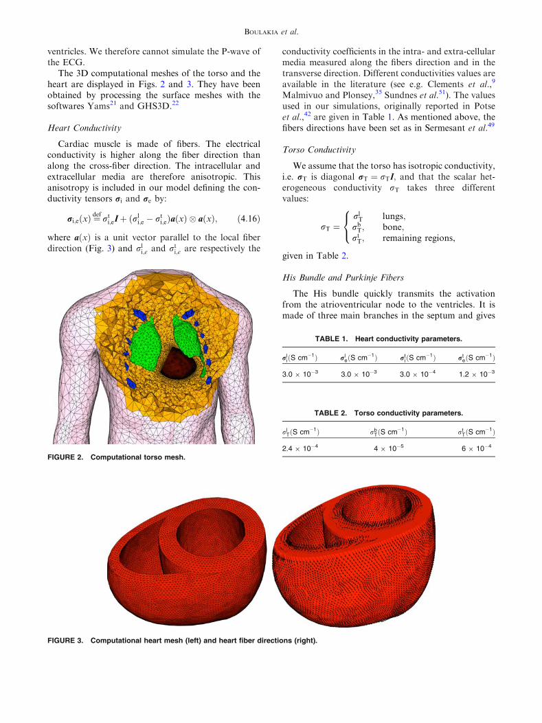
ventricles. We therefore cannot simulate the P-wave ofthe ECG.

The 3D computational meshes of the torso and theheart are displayed in Figs. 2 and 3. They have beenobtained by processing the surface meshes with thesoftwares Yams21 and GHS3D.22

Heart Conductivity

Cardiac muscle is made of fibers. The electricalconductivity is higher along the fiber direction thanalong the cross-fiber direction. The intracellular andextracellular media are therefore anisotropic. Thisanisotropy is included in our model defining the con-ductivity tensors ri and re by:

ri;eðxÞ ¼def

rti;eIþ ðrl

i;e � rti;eÞaðxÞ � aðxÞ; ð4:16Þ

where aðxÞ is a unit vector parallel to the local fiberdirection (Fig. 3) and rl

i;e and rti;e are respectively the

conductivity coefficients in the intra- and extra-cellularmedia measured along the fibers direction and in thetransverse direction. Different conductivities values areavailable in the literature (see e.g. Clements et al.,9

Malmivuo and Plonsey,35 Sundnes et al.51). The valuesused in our simulations, originally reported in Potseet al.,42 are given in Table 1. As mentioned above, thefibers directions have been set as in Sermesant et al.49

Torso Conductivity

We assume that the torso has isotropic conductivity,i.e. rT is diagonal rT ¼ rTI; and that the scalar het-erogeneous conductivity rT takes three differentvalues:

rT ¼rlT lungs;

rbT; bone;

rtT; remaining regions,

8<:

given in Table 2.

His Bundle and Purkinje Fibers

The His bundle quickly transmits the activationfrom the atrioventricular node to the ventricles. It ismade of three main branches in the septum and gives

FIGURE 2. Computational torso mesh.

FIGURE 3. Computational heart mesh (left) and heart fiber directions (right).

TABLE 1. Heart conductivity parameters.

rliðS cm�1Þ rl

eðS cm�1Þ rtiðS cm�1Þ rt

eðS cm�1Þ

3.0 9 10�3 3.0 9 10�3 3.0 9 10�4 1.2 9 10�3

TABLE 2. Torso conductivity parameters.

rlTðS cm�1Þ rb

TðS cm�1Þ rtTðS cm�1Þ

2.4 9 10�4 4 9 10�5 6 9 10�4

BOULAKIA et al.

rise to the thin Purkinje fibers in the ventricular mus-cle. The activation travels from the His bundle to theventricular muscle in about 40 ms. Interesting attemptsat modeling the His bundle and the Purkinje fibershave been presented in the literature (see e.g. Vigmondand Clements57). But a physiological model of this fastconduction network coupled to a 3D model of themyocardium raises many modeling and computationaldifficulties: the fiber network has to be manuallydefined whereas it cannot be non-invasively obtainedfrom classical imaging techniques; the results arestrongly dependent on the density of fibers which is aquantity difficult to determine; the time and the spacescales are quite different in the fast conduction net-work and in the rest of the tissue which can be chal-lenging from the computational standpoint.

To circumvent these issues, we propose to roughlymodel the Purkinje system by initializing the activationwith a (time-dependent) external volume current, actingon a thin subendocardial layer (both left and rightparts). The propagation speed of this initial activation isa parameter of the model (see the details in Appendix).Although this approach involves a strong simplificationof the reality, it allows a simple and quite accuratecontrol of the activation initialization, which is a fun-damental aspect in the simulation of correct ECGs.

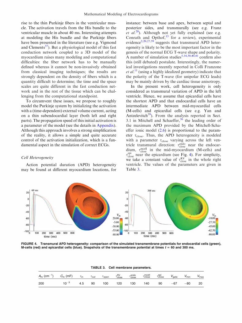
Cell Heterogeneity

Action potential duration (APD) heterogeneitymay be found at different myocardium locations, for

instance: between base and apex, between septal andposterior sides, and transmurally (see e.g. Franzet al.20). Although not yet fully explained (see e.g.Conrath and Opthof,13 for a review), experimentalevidence2,20,27,59 suggests that transmural APD heter-ogeneity is likely to be the most important factor in thegenesis of the normal ECG T-wave shape and polarity.A number of simulation studies5,14,30,40,41 confirm alsothis (still debated) postulate. Interestingly, the numer-ical investigations recently reported in Colli Franzoneet al.11 (using a highly idealized geometry) indicate thatthe polarity of the T-wave (for unipolar ECG leads)may be mainly driven by the cardiac tissue anisotropy.

In the present work, cell heterogeneity is onlyconsidered as transmural variation of APD in the leftventricle. Hence, we assume that epicardial cells havethe shortest APD and that endocardial cells have anintermediate APD between mid-myocardial cells(M-cells) and epicardial cells (see e.g. Yan andAntzelevitch59). From the analysis reported in Sect.3.1 in Mitchell and Schaeffer,36 the leading order ofthe maximum APD provided by the Mitchell-Scha-effer ionic model (2.6) is proportional to the param-eter sclose. Thus, the APD heterogeneity is modeledwith a parameter sclose varying across the left ven-tricle transmural direction: sendoclose near the endocar-dium, smcell

close in the mid-myocardium (M-cells) andsepiclose near the epicardium (see Fig. 4). For simplicity,we take a constant value of sRV

close in the whole rightventricle. The values of the parameters are given inTable 3.

FIGURE 4. Transmural APD heterogeneity: comparison of the simulated transmembrane potentials for endocardial cells (green),M-cells (red) and epicardial cells (blue). Snapshots of the transmembrane potential at times t 5 60 and 300 ms.

TABLE 3. Cell membrane parameters.

Am (cm�1) Cm (mF) sin sout sopen sRVclose sendo

close sclosemcell sclose

epi Vgate Vmin Vmax

200 10�3 4.5 90 100 120 130 140 90 �67 �80 20


Results

The ECGs are computed according to the standard12-lead ECG definition (see Malmivuo and Plonsey,35

for instance):

I¼defuTðLÞ� uTðRÞ; II¼defuTðFÞ� uTðRÞ;

III¼defuTðFÞ� uTðLÞ;

aVR¼def 32

uTðRÞ� uWð Þ; aVL¼def 32

uTðLÞ� uWð Þ; ð4:17Þ

aVF¼def 32

uTðFÞ� uWð Þ;

Vi¼defuTðViÞ� uW i¼ 1; . . . ;6;

where uW ¼def ðuTðLÞ þ uTðRÞ þ uTðFÞÞ=3 and the body

surface electrode locations L, R, F, fVigi¼1;...;6 areindicated in Fig. 5.

The simulated ECG obtained from RS is reported inFig. 6. Some snapshots of the corresponding bodysurface potential are depicted in Fig. 7. Compared to aphysiological ECG, the computed ECGhas someminorflaws. First, the T-wave amplitude is slightly lower thanexpected. Second, the electrical heart axis (i.e. the meanfrontal plane direction of the depolarization waveFIGURE 5. Torso domain: ECG leads locations.

FIGURE 6. Reference simulation: 12-lead ECG signals obtained by a strong coupling with the torso, including anisotropy andAPD heterogeneity. As usual, the units in the x- and y-axis are ms and mV, respectively.

BOULAKIA et al.

traveling through the ventricles during ventricularactivation) is about �40� whereas it should be between0� and 90� (see e.g. Aehlert1). This is probably due to atoo horizontal position of the heart in the thoracic

cavity. Third, in the precordial leads, the R-wave pre-sents abnormal (low) amplitudes in V1 and V2 and theQRS complex shows transition from negative to posi-tive polarity in V4 whereas this could be expected in V3.

FIGURE 7. Reference simulation: some snapshots of the body surface potentials at times t 5 10, 47, 70, 114, 239 and 265 ms(from left to right and top to bottom).


Despite that, the main features of a physiologicalECG can be observed. For example, the QRS-complexhas a correct orientation and a realistic amplitude ineach of the 12 leads. In particular, it is negative in leadV1and becomes positive in lead V6. Moreover, its durationis between 80 and 120 ms, which is the case of a healthysubject. The orientation and the duration of the T-waveare also satisfactory. To the best of our knowledge, this12-lead ECG is the most realistic ever published from afully based PDE/ODE 3D computational model.

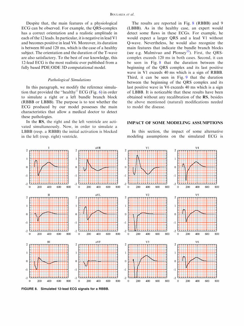
Pathological Simulations

In this paragraph, we modify the reference simula-tion that provided the ‘‘healthy’’ ECG (Fig. 6) in orderto simulate a right or a left bundle branch block(RBBB or LBBB). The purpose is to test whether theECG produced by our model possesses the maincharacteristics that allow a medical doctor to detectthese pathologies.

In the RS, the right and the left ventricle are acti-vated simultaneously. Now, in order to simulate aLBBB (resp. a RBBB) the initial activation is blockedin the left (resp. right) ventricle.

The results are reported in Fig. 8 (RBBB) and 9(LBBB). As in the healthy case, an expert woulddetect some flaws in these ECGs. For example, hewould expect a larger QRS and a lead V1 withoutQ-wave. Nevertheless, he would also recognize themain features that indicate the bundle branch blocks(see e.g. Malmivuo and Plonsey35). First, the QRS-complex exceeds 120 ms in both cases. Second, it canbe seen in Fig. 8 that the duration between thebeginning of the QRS complex and its last positivewave in V1 exceeds 40 ms which is a sign of RBBB.Third, it can be seen in Fig. 9 that the durationbetween the beginning of the QRS complex and itslast positive wave in V6 exceeds 40 ms which is a signof LBBB. It is noticeable that these results have beenobtained without any recalibration of the RS, besidesthe above mentioned (natural) modifications neededto model the disease.

IMPACT OF SOME MODELING ASSUMPTIONS

In this section, the impact of some alternativemodeling assumptions on the simulated ECG is

FIGURE 8. Simulated 12-lead ECG signals for a RBBB.

BOULAKIA et al.

investigated. This allows to assess to what extent themodeling assumptions involved in the RS are necessaryto obtain a meaningful ECG.

Heart–Torso Uncoupling

A common approach to reduce the computationalcomplexity of the RM consists in uncoupling thecomputation of (Vm, ue) and uT. This can be achievedby neglecting, in (2.10), the electrical torso feedback onthe cardiac region. That is, by replacing the couplingcondition (2.10)2 by

rerue � n ¼ 0; on R; ð5:18Þ

which amounts to work with an isolated heart domain(see e.g. Clements et al.,9 Potse et al.42).

As a result, the intracardiac quantities (Vm, ue)can be obtained, independently of uT, by solving(2.7) with initial condition (2.8) and insulating con-ditions

ri$Vm � nþ ri$ue � n ¼ 0; on R;re$ue � n ¼ 0; on R:

�ð5:19Þ

Thereafter, the torso potential uT is recovered bysolving (2.11) with

uT ¼ ue; on R;rT$uT � nT ¼ 0; on Cext;

�: ð5:20Þ

as boundary conditions. In other words, the uncoupledheart potential ue is transferred, from XH to XT,through the interface R (see Barr et al.,3 Shahidiet al.50).

Remark 5.1 Rather than interface based, as (5.20),most of the uncoupled approaches reported in theliterature are volume based (see Sect. 4.2.4 in Lineset al.,32 for a review). Thus, the torso potentials aregenerated by assuming a (multi-)dipole representationof the cardiac source, typically based on thetransmembrane potential gradient rVm (see e.g.Gulrajani,26 Pullan et al.44).

From the numerical point of view, the heart–torsouncoupling amounts to replace Step 4, in ‘‘Space andTime Discretization’’ section, by:

Solving for ðVnþ1m ; unþ1e Þ 2 Vh � Vh; withR

XHunþ1e ¼ 0:

FIGURE 9. Simulated 12-lead ECG signals for a LBBB.


Am

RXH

Cm

dt32V

nþ1m � 2Vn

m þ 12V

n�1m

� �/

þR

XHri$ Vnþ1

m þ unþ1� �

� $/

¼ Am

RXH

Iappðtnþ1Þ � Iion eVnþ1m ;wnþ1

� �� /;R

XHri þ reð Þ$unþ1e � $we þ

RXH

ri$Vnþ1m � $we ¼ 0;

8>>>><>>>>:

for all ð/;weÞ 2 Vh � Vh; withR

XHwe ¼ 0:

Then, once funþ1e g0�n�N�1 are available, the torsopotential is obtained by solving, for unþ1T 2 Zh;

unþ1T ¼ unþ1e ; on R;ZXT

rTrunþ1T � rwT ¼ 0; 8wT 2 Zh;0:ð5:21Þ

The remainder of this section discusses the impact ofthe uncoupled approach on ECG accuracy and com-putational cost.

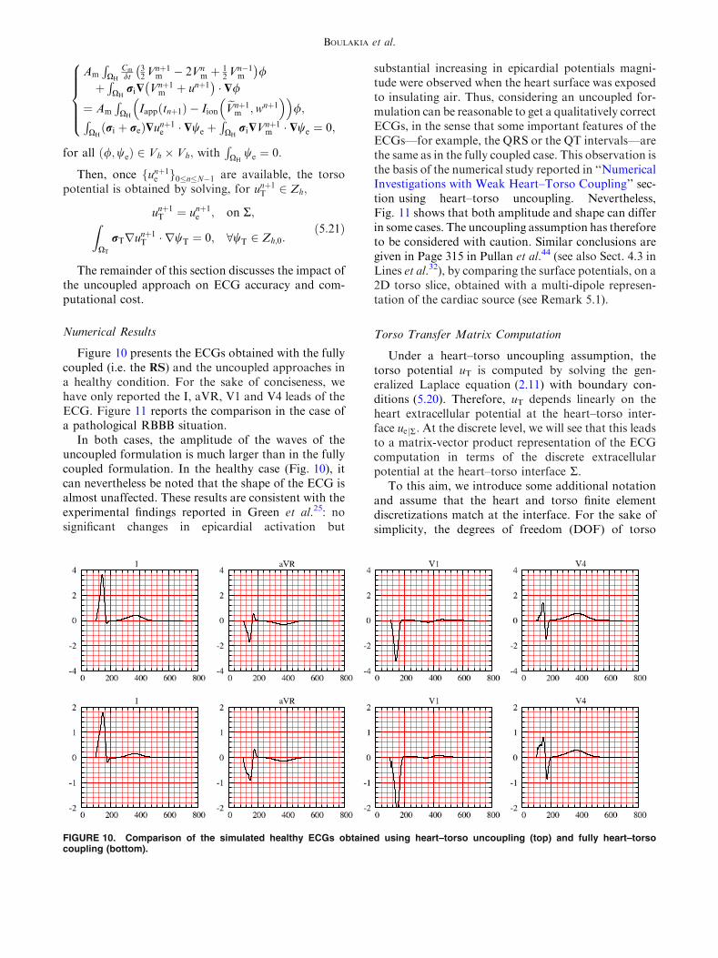
Numerical Results

Figure 10 presents the ECGs obtained with the fullycoupled (i.e. the RS) and the uncoupled approaches ina healthy condition. For the sake of conciseness, wehave only reported the I, aVR, V1 and V4 leads of theECG. Figure 11 reports the comparison in the case ofa pathological RBBB situation.

In both cases, the amplitude of the waves of theuncoupled formulation is much larger than in the fullycoupled formulation. In the healthy case (Fig. 10), itcan nevertheless be noted that the shape of the ECG isalmost unaffected. These results are consistent with theexperimental findings reported in Green et al.25: nosignificant changes in epicardial activation but

substantial increasing in epicardial potentials magni-tude were observed when the heart surface was exposedto insulating air. Thus, considering an uncoupled for-mulation can be reasonable to get a qualitatively correctECGs, in the sense that some important features of theECGs—for example, the QRS or the QT intervals—arethe same as in the fully coupled case. This observation isthe basis of the numerical study reported in ‘‘NumericalInvestigations with Weak Heart–Torso Coupling’’ sec-tion using heart–torso uncoupling. Nevertheless,Fig. 11 shows that both amplitude and shape can differin some cases. The uncoupling assumption has thereforeto be considered with caution. Similar conclusions aregiven in Page 315 in Pullan et al.44 (see also Sect. 4.3 inLines et al.32), by comparing the surface potentials, on a2D torso slice, obtained with a multi-dipole represen-tation of the cardiac source (see Remark 5.1).

Torso Transfer Matrix Computation

Under a heart–torso uncoupling assumption, thetorso potential uT is computed by solving the gen-eralized Laplace equation (2.11) with boundary con-ditions (5.20). Therefore, uT depends linearly on theheart extracellular potential at the heart–torso inter-face uejR: At the discrete level, we will see that this leadsto a matrix-vector product representation of the ECGcomputation in terms of the discrete extracellularpotential at the heart–torso interface R.

To this aim, we introduce some additional notationand assume that the heart and torso finite elementdiscretizations match at the interface. For the sake ofsimplicity, the degrees of freedom (DOF) of torso

FIGURE 10. Comparison of the simulated healthy ECGs obtained using heart–torso uncoupling (top) and fully heart–torsocoupling (bottom).

BOULAKIA et al.

potential are partitioned as xT ¼def ½xT;I; xT;R� 2 RnIþnR ;where xT;R denotes the heart–torso interface DOF andxT;I the remaining DOF. We denote by xejR 2 RnR theextracellular potential DOF at the heart–torso inter-face R. Finally, we assume that the 9 potential valuesgenerating the ECG (see ‘‘Results’’ section), sayxECG 2 R9; are obtained from the discrete torsopotential xT in terms of an interpolation operatorP 2 R9�nI ; so that

xECG ¼ PxT;I; ð5:22Þ

for instance, P can be a nodal value extraction of xT;I:On the other hand, from (5.21), the discrete torsopotential xT is solution to the following finite elementlinear system:

AII AIR

0 IRR

xT;IxT;R

¼ 0

xejR

: ð5:23Þ

Hence, by Gaussian elimination, we have that xT;I ¼�A�1II AIRxejR; and by inserting this expression in (5.22),we obtain

xECG ¼ �PA�1II AIR|fflfflfflfflfflfflffl{zfflfflfflfflfflfflffl}T

xejR:

Therefore, the ECG can be computed from the discreteextracellular potential at the heart torso interface, xejR;by a simple matrix-vector operation xECG ¼ TxejR;with T ¼def � PA�1II AIR:

There are different solutions to compute T:The naiveidea consisting of computing the matrixA�1II is of courseruled out. A reasonable and natural option is to com-pute matrix T by column (see Shahidi et al.50), i.e. by

evaluatingTei for i = 1, …, nR, where ei denotes the i-thcanonical vector of RnR : But each of these evaluationsinvolve the solution of system (5.23) with xejR ¼ ei; andtherefore the overall computational cost is proportionalto nR, which can be rather expensive (remember that nR

is the number of nodes on the heart–torso interface, andis therefore of the order of several thousands). In con-trast, a computation by row is much more efficient sinceit is only needed to evaluate TTei for i = 1, …, 9, whereei stands for the i-th canonical vector of R9: From thesymmetry of the finite element matrix,

TT ¼ �ATIRA

�TII PT ¼ �ARIA

�1II P

T:

Therefore, the matrix-vector product evaluation

TTei ¼ �ARI A�1II P

Tei|fflfflfflfflffl{zfflfflfflfflffl}xT;I

; ð5:24Þ

can be performed in two steps as follows. First, solvefor ½xT;I; xT;R� the discrete source problem (dependingon the linear operator P), with homogeneous Dirichletboundary condition on R:

AII AIR

0 IRR

xT;IxT;R

Ptei0

; ð5:25Þ

Second, from (5.24), evaluate the interface residual

TTei ¼ �ARIxT;I ¼ � ARI ARR½ � xT;IxT;R

:

Note that, TTei is nothing but the discrete current fluxthrough the heart–torso interface R, associated to thehomogeneous Dirichlet condition in (5.25).

FIGURE 11. Comparison of the simulated RBBB ECGs obtained using heart–torso uncoupling (top) and fully heart–torso cou-pling (bottom).


In this paper, all the numerical ECGs based onthe uncoupling conditions (5.19)–(5.20) have beenobtained using the matrix T presented in this para-graph (and this matrix has been computed by row).

Remark 5.2 If the operator P is a simple extractionof nodal values from the torso potential DOF, xT; eachevaluation TTei; for i = 1, …, 9, can be (formally)interpreted at the continuous level as a current fluxevaluation at R of the problem

divðrT$vÞ ¼ dxi ; in XT;v ¼ 0; on R;rT$v � nT ¼ 0; on Cext;

8<:

with dxi the Dirac’s delta function at the i-th point, xi;of torso potential recording on Cext.

Remark 5.3 Note that the transfer matrix T can becomputed ‘‘off-line’’, since it depends neither on timenor on solution in the heart. Nevertheless, this matrixhas to be recomputed when the torso conductivities aremodified or when dealing with dynamic torso meshes.

Table 4 reports the elapsed CPU time needed tosimulate an ECG with three different approaches. Asexpected, the uncoupling assumption significantlyreduces the computational cost of the ECG simulation,especially if the transfer matrix method is used torecover the torso potentials. Let us emphasize that, thelast two columns of Table 4 refer to the same problem(uncoupled formulation) solved with two differentalgorithms, whereas the problem corresponding to thefirst column (fully coupled formulation) is differentand a priori more accurate.

Study of the Monodomain Model

In the previous section we have investigated a sim-plifying modeling assumption that allows a uncoupledcomputation of the heart and torso potentials (Vm, ue)and uT.We nowdiscuss another simplification known asmonodomain approximation (see e.g. Clements et al.,9

Colli Franzone et al.12). Combined with a heart–torsouncoupling assumption, this approach leads to a fullydecoupled computation of Vm, ue and uT.

The next subsection investigates the implications, onECG modeling, of the general monodomain derivationproposed in Clements et al.9 and Colli Franzone

et al.,12 without any assumptions on the anisotropyratio of the intra- and extracellular conductivities. Theimpact of this approximation on the simulated ECG isthen illustrated in ‘‘Numerical Results with Heart–Torso Uncoupling’’ section, using the heart–torsouncoupling simplification.

The Monodomain Approximation

We assume that the intra- and extracellular local

conductivities rl;ti and rl;t

e are homogeneous (constant

in space). Let j ¼def ji þ je be the total current, flowing

into XH, and r ¼def ri þ re be the bulk conductivitytensor of the medium.

From (2.3) and (2.4), j ¼ �ri$ui � re$ue ¼�ri$Vm � r$ue; or, equivalently,

$ue ¼ �r�1ri$Vm � r�1j: ð5:26Þ

By inserting this expression in (2.7)1 and (2.9), weobtain

Am Cm@Vm


� div ri I� r�1ri

� �$Vm

� �¼ �div rir

�1j� �

þ AmIapp; in XH;ri I� r�1ri

� �$Vm � n ¼ rir

�1j � n; on R:

8<:

ð5:27Þ

On the other hand, ri I� r�1ri

� �¼ rir

�1ðr� riÞ ¼rir�1re: Therefore, by defining

ra ¼def

rir�1re; ð5:28Þ

the expression (5.27) reduces to

Am Cm@Vm


� div ra$Vmð Þ¼ �div rir

�1j� �

þ AmIapp; in XH;ra$Vm � n ¼ rir

�1j � n; on R:

8<: ð5:29Þ

Following Clements et al.9 and Colli Franzone et al.,12

we deduce from (4.16)

rir�1 ¼ ltIþ ðll � ltÞa� a; ð5:30Þ

with

ll ¼def ri

l

ril þ re

l

; lt ¼def ri

t

rit þ re

t

;

By setting e ¼def jlt � llj; we deduce from (5.30)

rir�1 ¼ ltIþOðeÞ: ð5:31Þ

As noticed in Clements et al.,9 e is a parameter thatmeasures the gap between the anisotropy ratios of theintra- and extracellular media. In general 0 £ e < 1,and for equal anisotropy ratios e = 0 so thatrir�1 ¼ ltI:Assuming e � 1, the expansion (5.31) can be

inserted into (5.29) by keeping the terms up to the zero

TABLE 4. Comparison of the elapsed CPU time (dimen-sionless) for the computation of the ECG.

Full coupling

Uncoupling

Laplace equation

Uncoupling

transfer matrix

60 4 1

BOULAKIA et al.

order. Thus, since lt is assumed to be constant, andusing (2.1) and (2.9), up to the zero order in e, theso-called monodomain approximation is obtained:

Am Cm@Vm


� div ra$Vmð Þ¼ AmIapp; in XH;

ra$Vm � n ¼ �lTre$ue � n; on R:

8<:

ð5:32Þ

Heart–torso full coupling. Under the full coupling con-ditions (2.10), Vm and ue cannot be determined indepen-dently from each other. Note that, in (5.32) the couplingbetween Vm and ue is fully concentrated on R, whereas inRM this coupling is also distributed inXH, through (2.7)1.Therefore, as soon as the heart and the torso are stronglycoupled, the monodomain approximation does not sub-stantially reduce the computational complexity withrespect to RM. Owing to this observation, we will notpursue the investigations on this approach.

Heart–torso uncoupling. Within the framework of‘‘Heart–Torso Uncoupling’’ section, the insulatingcondition (5.18) combined with (5.32) yields

Am Cm@Vm


� div ra$Vmð Þ¼ AmIapp; in XH;

ra$Vm � n ¼ 0; on R;

8<:

ð5:33Þ

which, along with (2.5), allows to compute Vm inde-pendently of ue. The extra-cellular potential can thenbe recovered, a posteriori, by solving

�div ri þ reð Þ$ueð Þ ¼ div ri$Vmð Þ; in XH;ri þ reð Þ$ue � n ¼ �ri$Vm � n; on R:

�

At last, the heart potentials are transferred to the torsoby solving (2.11) with (5.20), as in ‘‘Heart–TorsoUncoupling’’ section.

Therefore, the monodomain approximation (5.32)combined with a heart–torso uncoupling assumptionleads to a fully decoupled computation of Vm, ue anduT. The three systems of equations which have to besolved successively read:

1. Monodomain problem, decoupled Vm:

Am Cm@Vm

@t þ IionðVm;wÞ� ��div ra$Vmð Þ

¼ AmIapp; in XH;@w@t þ gðVm;wÞ ¼ 0; in XH;ra$Vm � n ¼ 0; on R:

8>>>><>>>>:

ð5:34Þ

2. Heart extracellular potential ue:

div ðriþreÞ$ueð Þ¼�divðri$VmÞ; in XH;ðriþreÞ$ue � n¼�ri$Vm � n; on R:

8<: ð5:35Þ

3. Torso potential uT:

div rT$uTð Þ ¼ 0; in XT;uT ¼ ue; on R;

rT$uT � nT ¼ 0; on Cext:

8<: ð5:36Þ

To sum up the discussion of this subsection on cansay that two levels of simplification can be consideredwith respect to RM: first, replacing the bidomainequations by the monodomain equations; second,replacing the full heart–torso coupling by an uncou-pled formulation. The first simplification significantlyreduces the computational effort only if the second oneis also assumed.

Numerical Results with Heart–Torso Uncoupling

Figure 12 shows the ECG signals obtained with thebidomain model (bottom) and the monodomainapproximation (top) in a healthy case, using the heart–torso uncoupling simplification. The simulated ECGsfor a RBBB pathological condition are given inFig. 13. These figures clearly show that the mostimportant clinical characteristics (e.g. QRS or QTdurations) are essentially the same in both approaches.

The first lead, in a healthy case, of both approachesare presented together in Fig. 14, for better compari-son. The relative difference on the first lead is only 4%in l2-norm. Thus, as far as the ECG is concerned,bidomain equations can be safely replaced by themonodomain approximation.

These observations are consistent with the conclu-sions of other studies based on isolated whole heartmodels.9,42 For instance, the numerical results reportedin Potse et al.42 show that the propagation of the acti-vation wave is only 2% faster in the bidomain modeland that the electrograms (point-wise values of theextra-cellular potential) are almost indistinguishable.

Isotropy

The impact of the conductivity anisotropy on theECG signals is now investigated. To this aim, thenumerical simulations of ‘‘Reference Simulation’’ sec-tion are reconsidered with isotropic conductivities, bysetting

rte¼rl

e¼3:0�10�3Scm�1; rti ¼rl

i¼3:0�10�3Scm�1:

Figure 15 (top) shows the corresponding ECG signals.The QRS and T waves have the same polarity than inthe anisotropic case, Fig. 15 (bottom). However, wecan clearly observe that the QRS-complex has asmaller duration and that the S-wave amplitude, inleads I and V4, is larger. The impact of anisotropy is


much more striking when dealing with pathologicalactivations. In Fig. 16, for instance, the simulatedECG signals for a RBBB pathology have beenreported with anisotropic and isotropic conductivities.Notice that the electrical signal is significantly dis-torted. In particular, the amplitude of the QRS com-plex is larger in the isotropic case (this observation alsoholds in the healthy case).

These numerical simulations show that anisotropyhas a major impact on the accuracy of ECG signals.

Meaningful ECG simulations have therefore to incor-porate this modeling feature (see also Colli Franzoneet al.11).

Cell Homogeneity

As mentioned in ‘‘Cell Heterogeneity’’ section, anheterogeneous coefficient sclose has been considered inRS to incorporate an APD gradient across the leftventricle transmural direction. In this paragraph, the

FIGURE 12. Simulated normal ECG with heart–torso uncoupling: monodomain (top) and bidomain (bottom) models.

FIGURE 13. Simulated ECG for a RBBB pathology with heart–torso uncoupling: monodomain (top) and bidomain (bottom)models.

BOULAKIA et al.

myocardium is assumed to have homogeneous cells.The ECG signals corresponding to a constant APD inthe whole heart, obtained with sclose = 140 ms, arereported in Fig. 17.

Note that now, in the bipolar lead (I), the T-wavehas an opposite polarity with respect to the RS and towhat is usually observed in normal ECGs. Indeed,without transmural APD heterogeneity, the repolari-zation and the depolarization waves travel in the samedirection, which leads to the discordant polarity,between the QRS and the T waves, observed in lead I.On the contrary, the unipolar leads (aVR, V1 and V4)

present a similar polarity, irrespectively of the ADPheterogeneity (see also Colli Franzone et al.11).

As a result, as also noticed in Boulakia et al.,5 Kelleret al.,30 and Potse et al.,40,41 transmural APD hetero-geneity is a major ingredient in the simulation of acomplete 12-lead ECG with physiological T-wavepolarities.

Capacitive and Resistive Effect of the Pericardium

The coupling conditions (2.10) are formallyobtained in Krassowska and Neu31 using an homoge-nization procedure. In that reference, a perfect elec-trical coupling is assumed between the heart and thesurrounding tissues.

It might be interesting to consider more generalcoupling conditions. For instance, by assuming thatthe pericardium (the double-walled sac containing theheart) might induce a resistor–capacitor effect. Thiscan be a way to model pathological conditions—e.g. pericarditis, when the pericardium becomesinflamed—or to take into account the fact that, even ina healthy situation, the heart–torso coupling can bemore complex. Thus, we propose to generalize (2.10),by introducing the following resistor–capacitor (R–C)coupling conditions:

RprT$uT � n ¼ RpCp@ðue�uTÞ

@t þ ðue � uTÞ; on R;re$ue � n ¼ rT$uT � n; on R;

�

ð5:37Þ

where Cp and Rp stand for the capacitance and resis-tance of the pericardium, respectively. Note that, theclassical relations (2.10) can be recovered from (5.37)

FIGURE 14. First ECG lead: bidomain and monodomainmodels with heart–torso uncoupling.

FIGURE 15. ECG signals: isotropic conductivities (top), anisotropic conductivities (bottom).


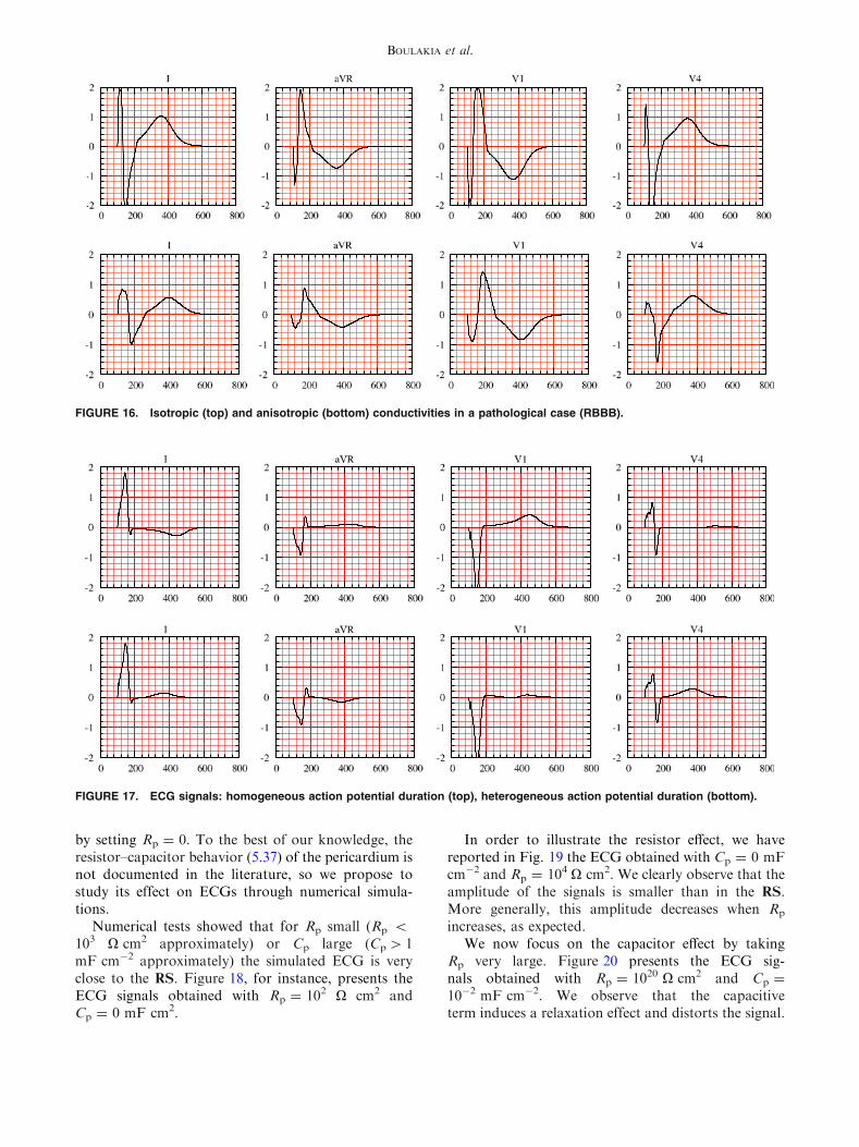
by setting Rp = 0. To the best of our knowledge, theresistor–capacitor behavior (5.37) of the pericardium isnot documented in the literature, so we propose tostudy its effect on ECGs through numerical simula-tions.

Numerical tests showed that for Rp small (Rp <

103 X cm2 approximately) or Cp large (Cp > 1mF cm�2 approximately) the simulated ECG is veryclose to the RS. Figure 18, for instance, presents theECG signals obtained with Rp = 102 X cm2 andCp = 0 mF cm2.

In order to illustrate the resistor effect, we havereported in Fig. 19 the ECG obtained with Cp = 0 mFcm�2 and Rp = 104 X cm2. We clearly observe that theamplitude of the signals is smaller than in the RS.More generally, this amplitude decreases when Rp

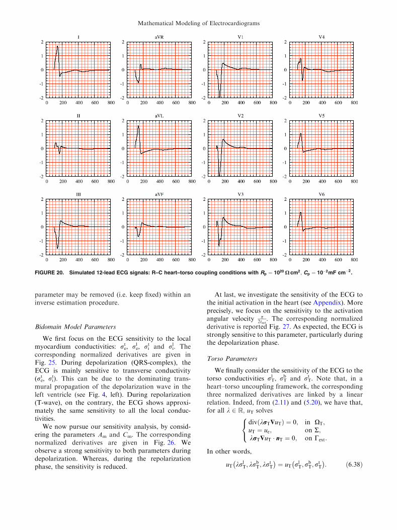
increases, as expected.We now focus on the capacitor effect by taking

Rp very large. Figure 20 presents the ECG sig-nals obtained with Rp = 1020 X cm2 and Cp =

10�2 mF cm�2. We observe that the capacitiveterm induces a relaxation effect and distorts the signal.

FIGURE 16. Isotropic (top) and anisotropic (bottom) conductivities in a pathological case (RBBB).

FIGURE 17. ECG signals: homogeneous action potential duration (top), heterogeneous action potential duration (bottom).

BOULAKIA et al.

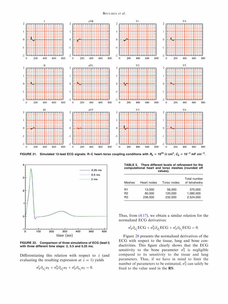
In particular, the T-wave is inverted in all the ECGleads and the S-wave duration is larger than for theRS. At last, Fig. 21 shows that for very small values ofCp the amplitude of the ECG is also very small. Thiscan be formally explained by the fact that, in thiscase, condition (5.37)1 approximately becomesrTruT � n ¼ 0 on R: no heart information is trans-ferred to the torso, leading to very low ECG signals.

NUMERICAL INVESTIGATIONS WITH WEAK

HEART–TORSO COUPLING

In this section, we investigate the ECG sensitivityto the time and space discretizations and to the heartand torso model parameters. To carry out thesestudies at a reasonable computational cost, we con-sider the heart–torso uncoupling. Although we havenoticed (in ‘‘Heart–Torso Uncoupling’’ section) thatuncoupling may affect the ECG accuracy in somecases, we can expect that the conclusions of thesensitivity analysis remain still valid under this sim-plification.

Time and Space Convergence

In this section, we are not interested in the conver-gence of the whole solution of the RM with respectto the space and time discretization parameters, butrather in the convergence of the ECG which is hereconsidered as the quantity of interest.

Time Convergence

In Fig. 22, we present the first ECG lead (lead I)obtained for three different time-step sizes dt = 0.25,0.5 and 2 ms. The l2-norm of the relative differencewith the result obtained with dt = 0.25 ms is 10%when dt = 2 ms and 2.0% when dt = 0.5 ms.

Space Convergence

Three different levels of refinements are consideredfor the heart and the torso meshes, as shown inTable 5. The finite element meshes used in the RS arethe R2. In Fig. 23, we report the first lead of the ECGsobtained for these simulations.

Although the whole solution might not be fullyconverged within the heart, we can observe that the

FIGURE 18. Simulated 12-lead ECG signals: R–C heart–torso coupling conditions with Rp ¼ 102 X cm2;Cp ¼ 0 mF cm�2.


quantity of interest—namely the ECG—is almostunaffected by the last refinement. Therefore, in a goal-oriented refinement framework, the solution mayindeed be considered as converged.

Sensitivity to Model Parameters

In this section, we study the sensitivity of ECG tosome model parameters. This is fundamental step priorto addressing its estimation (see e.g. Boulakia et al.6)using data assimilation techniques.

Suppose that a1, a2, …, ap are parameters the ECGdepends upon, i.e.

ECG ¼ ECG a1; a2; . . . ; ap� �

:

The ECG sensitivity to parameter ai can then beapproximated as

@aiECG a1;a2;...;ap� �

�ECGða1;a2;...;ð1þeÞai;...;apÞ�ECGða1;a2;...;apÞeai

;

where e is a small parameter, in our case 10�6 £e £ 10�4 gives a good approximation. Instead of@aiECG a1; a2; . . . ; ap

� �we consider the normalized

value ai@aiECG a1; a2; . . . ; ap� �

, which allows to com-pare the sensitivity irrespectively of the parameterscales. In the next paragraphs, we provide time evo-lution of this scaled derivative, evaluated around theparameters used in the RS. Once more, for the sake ofconciseness, we focus on the first ECG lead.

Ionic Model Parameters

In this paragraph, we investigate the sensitivity ofthe ECG to the Mitchell-Schaeffer parameters. InFig. 24, we have reported the normalized derivativeswith respect to sin, sout, sopen or sclose. The high ECGsensitivity to sin is clearly visible, particularly duringthe QRS-complex. The sensitivity to sout is moderateboth during the depolarization and depolarizationphases. As expected, the sensitivity to sclose is onlyrelevant during repolarization. Interestingly, the sen-sitivity to sopen is relatively small. Therefore, this

FIGURE 19. Simulated 12-lead ECG signals: R–C heart–torso coupling conditions with Rp = 104 X cm2;Cp = 0 mF cm�2.

BOULAKIA et al.

parameter may be removed (i.e. keep fixed) within aninverse estimation procedure.

Bidomain Model Parameters

We first focus on the ECG sensitivity to the localmyocardium conductivities: re

t, rel , ri

t and ril. The

corresponding normalized derivatives are given inFig. 25. During depolarization (QRS-complex), theECG is mainly sensitive to transverse conductivity(re

t, rit). This can be due to the dominating trans-

mural propagation of the depolarization wave in theleft ventricle (see Fig. 4, left). During repolarization(T-wave), on the contrary, the ECG shows approxi-mately the same sensitivity to all the local conduc-tivities.

We now pursue our sensitivity analysis, by consid-ering the parameters Am and Cm. The correspondingnormalized derivatives are given in Fig. 26. Weobserve a strong sensitivity to both parameters duringdepolarization. Whereas, during the repolarizationphase, the sensitivity is reduced.

At last, we investigate the sensitivity of the ECG tothe initial activation in the heart (see Appendix). Moreprecisely, we focus on the sensitivity to the activationangular velocity p

2tact. The corresponding normalized

derivative is reported Fig. 27. As expected, the ECG isstrongly sensitive to this parameter, particularly duringthe depolarization phase.

Torso Parameters

We finally consider the sensitivity of the ECG to thetorso conductivities rT

l , rTb and rT

t . Note that, in aheart–torso uncoupling framework, the correspondingthree normalized derivatives are linked by a linearrelation. Indeed, from (2.11) and (5.20), we have that,for all k 2 R; uT solves

div krT$uTð Þ ¼ 0; in XT;uT ¼ ue; on R;krT$uT � nT ¼ 0; on Cext:

8<:

In other words,

uT krlT; krb

T; krtT

� �¼ uT rl

T; rbT; r

tT

� �: ð6:38Þ

FIGURE 20. Simulated 12-lead ECG signals: R–C heart–torso coupling conditions with Rp ¼ 1020 X cm2; Cp ¼ 10�2mF cm�2.


Differentiating this relation with respect to k (andevaluating the resulting expression at k = 1) yields

rlT@rl

TuT þ rb

T@rbTuT þ rt

T@rtTuT ¼ 0:

Thus, from (4.17), we obtain a similar relation for thenormalized ECG derivatives:

rlT@rl

TECGþ rb

T@rbTECGþ rt

T@rtTECG ¼ 0:

Figure 28 presents the normalized derivatives of theECG with respect to the tissue, lung and bone con-ductivities. This figure clearly shows that the ECGsensitivity to the bone parameter rT

b is negligiblecompared to its sensitivity to the tissue and lungparameters. Thus, if we have in mind to limit thenumber of parameters to be estimated, rT

b can safely befixed to the value used in the RS.

FIGURE 21. Simulated 12-lead ECG signals: R–C heart–torso coupling conditions with Rp 5 1020 X cm2, Cp 5 1024 mF cm22.

FIGURE 22. Comparison of three simulations of ECG (lead I)with three different time steps: 2, 0.5 and 0.25 ms.

TABLE 5. There different levels of refinement for thecomputational heart and torso meshes (rounded off

values).

Meshes Heart nodes Torso nodes

Total number

of tetrahedra

R1 13,000 56,000 370,000

R2 80,000 120,000 1,080,000

R3 236,000 232,000 2,524,000

BOULAKIA et al.

CONCLUSION

A fully PDE/ODE based mathematical model forthe numerical simulation of ECGs has been described.The electrical activity of the heart is based on thecoupling of the bidomain equations with theMitchell-Schaeffer phenomenological ionic model,including anisotropic conductivities and transmuralAPD heterogeneity. This system of equations has beencoupled to a generalized Laplace equation in the torso,

with inhomogeneous conductivity (bone, lungs andremaining tissue). A detailed description of the differentalgorithms used for the numerical solution of theresulting ECG model has been also provided.

Our approach has several limitations: we did notconsider the atria, which prevents us from computingthe P wave of the ECG; the cell model being phenom-enological, it cannot handle complex ionic interactions;the effect of the blood flow on the ECG was neglected;the geometry of the ventricles were simplified.

FIGURE 23. Comparison of three simulations of ECG (lead I),using three different levels of mesh refinement (see Table 5).

FIGURE 24. Normalized ECG sensitivity to sin, sout, sopen andsclose.

FIGURE 25. Normalized ECG sensitivity to the local myo-cardium conductivities: re

t , rel , ri

t and rli.

FIGURE 26. Normalized ECG sensitivity to Am and Cm.


Despite the above mentioned limitations, we wereable to compute a satisfactory healthy 12-lead ECG,with a limited number a parameters. To the best of ourknowledge, this constitutes a breakthrough in themodeling of ECGs with partial differential equations.Moreover, for a pathological situation correspondingto a bundle branch block, our simulations have pro-vided an ECG which satisfies the typical criteria usedby medical doctors to detect this pathology. This

shows, in particular, that our numerical model havesome predictive features.

In a second part, we have studied the impact ofsome modeling assumptions on the ECGs. The mainconclusions of this investigation are the following:

1. As far as the general shape of the ECGs is con-cerned, heart–torso uncoupling can be consid-ered. The level of accuracy obtained withuncoupling is probably sufficient in severalapplications, which may explain why this sim-plification is so widespread in the literature.Nevertheless, our numerical results have clearlypointed out that the amplitudes of the ECGsignals obtained via uncoupling and full cou-pling can significantly differ. We therefore rec-ommend to carefully check in each specificsituations whether the uncoupling approxima-tion is acceptable or not.

2. In agreement with other studies, we noticedthat cell heterogeneity and fiber anisotropyhave an important impact on the ECG and,therefore, cannot be neglected.

3. The bidomain equations can apparently besafely replaced by the monodomain approxi-mation (5.32). Nevertheless, even with thissimplification, the transmembrane potentialVm and the extracellular potential ue still haveto be solved simultaneously when the heart andthe torso are fully coupled. Therefore, to bereally attractive, the monodomain simplifica-tion (5.32) has to come with a heart-torsouncoupling approximation, which (as men-tioned above) can affect the ECG. An alter-native can be to neglect the boundary couplingin (5.32) while keeping ue and uT fully coupled(see e.g. Potse et al.43 In a pure propagationframework, i.e. without extracellular pacing,numerical experiments suggest that thisapproach can provide accurate ECG signals.

4. We have proposed a new heart–torso couplingcondition which takes into account possiblecapacitive and resistive effects of the pericar-dium. We did not find in the literature any evi-dence of these effects and our results show that itdoes not seem necessary to include them in orderto get realistic healthy ECGs. Nevertheless,these coupling conditions might be relevant insome pathologies affecting the pericardial sacand the simulations we provided to illustratethese effects might be useful for future works.

5. At last, a sensitivity analysis has shown that themost critical parameters of the bidomain modelare Cm, Am, the angular velocity of the acti-vation wave and the transverse conductivities

FIGURE 27. Normalized ECG sensitivity to the activationangular velocity.

FIGURE 28. Normalized ECG sensitivity to rlT; rb

T and rtT.

BOULAKIA et al.

rit and re

t. As regards the ECG sensitivity to theionic model parameters, we have noticed aextreme sensitivity of the QRS-complex tothe parameter sin and a high sensitivity of theT-wave to the parameter sclose. Moreover, wehave also observed that the ECG sensitivity tothe torso conductivity parameters is less sig-nificant than to the heart model parameters.

To conclude, our main concern during this studywas to build a model rich enough to provide realisticECGs and simple enough to be easily parametrized. Inspite of its shortcomings, the proposed approachessentially fulfills these requirements and is therefore agood candidate to address inverse problems. This willbe investigated in future works.

APPENDIX: EXTERNAL STIMULUS

In order to initiate the spread of excitation within themyocardium,we apply a given volume current density toa thin subendocardial layer of the ventricles during asmall period of time tact. In the left ventricle, this thinlayer (1.6 mm) of external activation is given by

S ¼def fðx; y; zÞ 2 XH=c1 � ax2 þ by2 þ cz2 � c2g;

where a, b, c, c1 and c2 are given constants, withc1 < c2, see Fig. 29. The source current Iapp, involvedin (2.7), is then parametrized as follows:

Iappðx; y; z; tÞ ¼ I0ðx; y; zÞvSðx; y; zÞv½0;tact�ðtÞwðx; z; tÞ;

where

I0ðx; y; zÞ ¼def iappc2

c2 � c1� 1

c2 � c1ax2 þ by2 þ cz2� �

;

with iapp the amplitude of the external appliedstimulus,

vSðx; y; zÞ ¼def 1 if ðx; y; zÞ 2 S;

0 if ðx; y; zÞ j2S;

�

v½0;tact�ðtÞ ¼def 1 if t 2 ½0; tact�;

0 if t j2 ½0; tact�;

�

wðx; z; tÞ ¼def1 if atan x�x0

z�z0

� �� aðtÞ;

0 if atan x�x0z�z0

� �>aðtÞ;

8><>:

the activated angle aðtÞ ¼def tp2tact

and tact = 10ms. Theactivation current in the right ventricle is built in asimilar fashion.

ACKNOWLEDGMENTS

This work was partially supported by INRIAthrough its large scope initiative CardioSense3D. Theauthors wish to thank Elsie Phe (INRIA) for her workon the anatomical models and meshes, and MichelSorine (INRIA) for valuable discussions regarding, inparticular, the heart–torso transmission conditions.

REFERENCES

1Aehlert, B. ECGs Made Easy (3rd ed.). Mosby Jems,Elsevier, 2006.2Antzelevitch, C. Cellular basis for the repolarization wavesof the ECG. Ann. N. Y. Acad. Sci. 1080:268–281, 2006.3Barr, R. C., M. Ramsey III, and M. S. Spach. Relatingepicardial to body surface potential distributions by meansof transfer coefficients based on geometry measurements.IEEE Trans. Biomed. Eng. 24(1):1–11, 1977.4Beeler, G., and H. Reuter. Reconstruction of the actionpotential of ventricular myocardial fibres. J. Physiol.(Lond.) 268:177–210, 1977.5Boulakia, M., M. A. Fernandez, J.-F. Gerbeau, andN. Zemzemi. Towards the numerical simulation of elec-trocardiograms. In: Functional Imaging and Modeling ofthe Heart, Vol. 4466 of Lecture Notes in Computer Sci-ence, edited by F. B. Sachse and G. Seemann. Springer-Verlag, 2007, pp. 240–249.6Boulakia, M., M. A. Fernandez, J.-F. Gerbeau, andN. Zemzemi. Direct and inverse problems in electrocardi-ography. AIP Conf. Proc. 1048(1):113–117, 2008.7Boulakia, M., M. A. Fernandez, J.-F. Gerbeau, andN. Zemzemi. A coupled system of PDEs and ODEs arisingin electrocardiograms modelling. Appl. Math. Res. Exp.2008(abn002):28, 2008.8Buist, M., and A. Pullan. Torso coupling techniques for theforward problem of electrocardiography. Ann. Biomed.Eng. 30(10):1299–1312, 2002.9Clements, J., J. Nenonen, P. K. J. Li, and B. M. Horacek.Activation dynamics in anisotropic cardiac tissue viadecoupling. Ann. Biomed. Eng. 32(7):984–990, 2004.

FIGURE 29. Geometrical description of the external stimulus(plane cut y 5 0).


10Colli Franzone, P., and L. F. Pavarino. A parallel solverfor reaction-diffusion systems in computational electro-cardiology. Math. Models Methods Appl. Sci. 14(6):883–911, 2004.

11Colli Franzone, P., L. F. Pavarino, S. Scacchi, andB. Taccardi. Effects of anisotropy and transmural hetero-geneity on the T-wave polarity of simulated electrograms.In: Functional Imaging and Modeling of the Heart,Vol. 5528 of Lecture Notes in Computer Science, edited byN. Ayache, H. Delingette, and M. Sermesant. Springer-Verlag, 2009, pp. 513–523.

12Colli Franzone, P., L. F. Pavarino, and B. Taccardi. Sim-ulating patterns of excitation, repolarization and actionpotential duration with cardiac bidomain and monodo-main models. Math. Biosci. 197(1):35–66, 2005.

13Conrath, C. E., and T. Opthof. Ventricular repolarization:an overview of (patho)physiology, sympathetic effects andgenetic aspects. Prog. Biophys. Mol. Biol. 92(3):269–307,2006.

14di Bernardo, D., and A. Murray. Modelling cardiac repo-larisation for the study of the T wave: effect of repolari-sation sequence. Chaos Solitons Fractals 13(8):1743–1748,2002.

15Djabella, K., and M. Sorine. Differential model of theexcitation-contraction coupling in a cardiac cell for multi-cycle simulations. In: EMBEC’05, Vol. 11. Prague, 2005,pp. 4185–4190.

16Ebrard, G., M. A. Fernandez, J.-F. Gerbeau, F. Rossi, andN. Zemzemi. From intracardiac electrograms to electrocar-diograms. models and metamodels. In: Functional Imagingand Modeling of the Heart, Vol. 5528 of Lecture Notes inComputer Science, edited by N. Ayache, H. Delingette, andM. Sermesant. Springer-Verlag, 2009, pp. 524–533.

17Ethier, M., and Y. Bourgault. Semi-implicit time-discreti-zation schemes for the bidomain model. SIAM J. Numer.Anal. 46:2443, 2008.

18Fenton, F., and A. Karma. Vortex dynamics in three-dimensional continuous myocardium with fiber rotation:filament instability and fibrillation. Chaos 8(1):20–47, 1998.

19Fitzhugh, R. Impulses and physiological states in theoreticalmodels of nerve membrane. Biophys. J. 1:445–465, 1961.

20Franz, M. R., K. Bargheer, W. Rafflenbeul, A. Haverich,and P. R. Lichtlen. Monophasic action potential mappingin human subjects with normal electrocardiograms: directevidence for the genesis of the T wave. Circulation75(2):379–386, 1987.

21Frey, P. Yams: a fully automatic adaptive isotropic surfaceremeshing procedure. Technical report 0252, Inria, Roc-quencourt, France, November 2001.

22George, P. L., F. Hecht, and E. Saltel. Fully automaticmesh generator for 3d domains of any shape. ImpactComput. Sci. Eng. 2:187–218, 1990.

23Gerardo-Giorda, L., L. Mirabella, F. Nobile, M. Perego,and A. Veneziani. A model-based block-triangular pre-conditioner for the bidomain system in electrocardiology.J. Comput. Phys. 228(10):3625–3639, 2009.

24Goldberger, A. L. Clinical Electrocardiography: A Sim-plified Approach (7th ed.). Mosby–Elsevier, 2006.

25Green, L. S., B. Taccardi, P. R. Ershler, and R. L. Lux.Epicardial potential mapping. effects of conducting mediaon isopotential and isochrone distributions. Circulation84(6):2513–2521, 1991.

26Gulrajani, R. M. Models of the electrical activity of theheart and computer simulation of the electrocardiogram.Crit. Rev. Biomed. Eng. 16(1):1–6, 1988.

27Higuchi, T., and Y. Nakaya. T wave polarity related to therepolarization process of epicardial and endocardial ven-tricular surfaces. Am. Heart J. 108(2):290–295, 1984.

28Huiskamp, G. Simulation of depolarization in a mem-brane-equations-based model of the anisotropic ventricle.EEE Trans. Biomed. Eng., 5045(7):847–855, 1998.

29Irons, B., and R. C. Tuck. A version of the aitken accel-erator for computer implementation. Int. J. Numer. Meth-ods Eng., 1:275–277, 1969.

30Keller, D. U. J., G. Seemann, D. L. Weiss, D. Farina,J. Zehelein, and O. Dossel. Computer based modeling ofthe congenital long-qt 2 syndrome in the visible man torso:from genes to ECG. In: Proceedings of the 29th AnnualInternational Conference of the IEEE EMBS, 2007,pp. 1410–1413.

31Krassowska, W., and J. C. Neu. Effective boundary con-ditions for syncitial tissues. IEEE Trans. Biomed. Eng.41(2):143–150, 1994.

32Lines, G. T., M. L. Buist, P. Grottum, A. J. Pullan,J. Sundnes, and A. Tveito. Mathematical models andnumerical methods for the forward problem in cardiacelectrophysiology. Comput. Vis. Sci. 5(4):215–239, 2003.

33Luo, C., and Y. Rudy. A dynamic model of the cardiacventricular action potential. I. Simulations of ionic currentsand concentration changes. Circ. Res. 74(6):1071–1096,1994.

34Luo, C. H., and Y. Rudy. A model of the ventricular car-diac action potential. depolarisation, repolarisation,andtheir interaction. Circ. Res. 68(6):1501–1526, 1991.

35Malmivuo, J., and R. Plonsey. Bioelectromagnetism.Principles and Applications of Bioelectric and BiomagneticFields. New York: Oxford University Press, 1995.

36Mitchell, C. C., and D. G. Schaeffer. A two-current modelfor the dynamics of cardiac membrane. Bull. Math. Biol.65:767–793, 2003.

37Neu, J. C., and W. Krassowska. Homogenization ofsyncytial tissues. Crit. Rev. Biomed. Eng. 21(2):137–199,1993.

38Noble, D., A. Varghese, P. Kohl, and P. Noble. Improvedguinea-pig ventricular cell model incorporating a diadicspace, ikr and iks, and length- and tension-dependentprocesses. Can. J. Cardiol. 14(1):123–134, 1998.

39Pennacchio, M., G. Savare, and P. Colli Franzone. Mul-tiscale modeling for the bioelectric activity of the heart.SIAM J. Math. Anal. 37(4):1333–1370, 2005.

40Potse, M., G. Baroudi, P. A. Lanfranchi, and A. Vinet.Generation of the t wave in the electrocardiogram: lessonsto be learned from long-QT syndromes. In: CanadianCardiovascular Congress, 2007.

41Potse, M., B. Dube, and M. Gulrajani. ECG simulationswith realistic human membrane, heart, and torso models.In: Proceedings of the 25th Annual Intemational Confer-ence of the IEEE EMBS, 2003, pp. 70–73.

42Potse, M., B. Dube, J. Richer, A. Vinet, and R. M.Gulrajani. A comparison of monodomain and bidomainreaction-diffusion models for action potential propagationin the human heart. IEEE Trans. Biomed. Eng. 53(12):2425–2435, 2006.

43Potse, M., B. Dube, and A. Vinet. Cardiac anisotropy inboundary-element models for the electrocardiogram. Med.Biol. Eng. Comput. doi:10.1007/s11517-009-0472-x.

44Pullan, A. J., M. L. Buist, and L. K. Cheng. Mathemati-cally modelling the electrical activity of the heart: from cellto body surface and back again. Hackensack, NJ: WorldScientific Publishing Co. Pte. Ltd., 2005.

BOULAKIA et al.

http://dx.doi.org/10.1007/s11517-009-0472-x

45Quarteroni, A., R. Sacco, and F. Saleri. Numerical Math-ematics, Vol. 37 of Texts in Applied Mathematics (2nd ed.).Berlin: Springer-Verlag, 2007.

46Quarteroni, A., and A. Valli. Domain decompositionmethods for partial differential equations. In: NumericalMathematics and Scientific Computation. New York: TheClarendon Press, Oxford University Press, Oxford SciencePublications, 1999.

47Sachse, F. B. Computational Cardiology: Modeling ofAnatomy, Electrophysiology, and Mechanics. Springer-Verlag, 2004.

48Scacchi, S., L. F. Pavarino, and I. Milano. MultilevelSchwarz and Multigrid preconditioners for the Bidomainsystem. Lect. Notes Comput. Sci. Eng. 60:631, 2008.

49Sermesant, M., Ph. Moireau, O. Camara, J. Sainte-Marie,R. Andriantsimiavona, R. Cimrman, D. L. Hill, D.Chapelle, and R. Razavi. Cardiac function estimation frommri using a heart model and data assimilation: advancesand difficulties. Med. Image Anal. 10(4):642–656, 2006.

50Shahidi, A. V., P. Savard, and R. Nadeau. Forward andinverse problems of electrocardiography: modeling andrecovery of epicardial potentials in humans. IEEE Trans.Biomed. Eng. 41(3):249–256, 1994.

51Sundnes, J., G. T. Lines, X. Cai, B. F. Nielsen, K.-A.Mardal, and A. Tveito. Computing the Electrical Activityin the Heart. Springer-Verlag, 2006.

52Sundnes, J., G. T. Lines, K.-A. Mardal, and A. Tveito.Multigrid block preconditioning for a coupled system ofpartial differential equations modeling the electrical activityin the heart. Comput. Methods Biomech. Biomed. Eng.5(6):397–409, 2002.

53Toselli, A., and O. Widlund. Domain Decomposition Meth-ods—Algorithms and Theory, Vol. 34 of Springer Series inComputational Mathematics. Berlin: Springer-Verlag, 2005.

54Trudel, M.-C., B. Dube, M. Potse, R. M. Gulrajani, andL. J. Leon. Simulation of qrst integral maps with a mem-brane-based computer heart model employing parallel pro-cessing. IEEE Trans. Biomed. Eng. 51(8):1319–1329, 2004.

55Tung, L. A Bi-Domain Model for Describing IschemicMyocardial D–C potentials. Ph.D. thesis, MIT, 1978.

56van Capelle, F. H., and D. Durrer. Computer simulation ofarrhythmias in a network of coupled excitable elements.Circ. Res. 47:453–466, 1980.

57Vigmond, E. J., and C. Clements. Construction of a com-puter model to investigate sawtooth effects in the purkinjesystem. IEEE Trans. Biomed. Eng. 54(3):389–399, 2007.

58Vigmond, E. J., R. Weber dos Santos, A. J. Prassl, M. Deo,and G. Plank. Solvers for the cardiac bidomain equations.Prog. Biophys. Mol. Biol. 96(1–3):3–18, 2008.

59Yan, G.-X., and C. Antzelevitch. Cellular basis for thenormal T wave and the electrocardiographic manifestationsof the long-QT syndrome. Circulation 98:1928–1936, 1998.


Documents

Mathematical Modeling of Electrocardiograms: A … · Mathematical Modeling of Electrocardiograms: A Numerical ... ECG simulator can also be useful in building a ... Mathematical