GMRC 2015 LiDAR and Orthoimagery Project December 8, 2015 Quantum Spatial, Inc. 523 Wellington Way, Suite 375 Lexington, KY 40503. 859-277-8700 Prepared by: GMRC 2015 LiDAR and Orthoimagery

Submitted: December 8, 2015

Quantum Spatial, Inc523 Wellington Way, Suite 375Lexington, KY 40503859-277-8700

Prepared by:

GMRC 2015 LiDAR and Orthoimagery Project

December 8, 2015Page ii of iiiGMRC2015 LiDAR & Ortho Project

Project Report

Contents1. Summary / Scope ...............................................................................................................................................1

1.1. Summary .................................................................................................................................................11.2. Scope ......................................................................................................................................................11.3. Location / Coverage ..........................................................................................................................31.4.Duration .................................................................................................................................................31.5. Issues .....................................................................................................................................................31.6. Deliverables .........................................................................................................................................3

2. Planning / Equipment ......................................................................................................................................62.1. Flight Planning ....................................................................................................................................62.2. LiDAR Sensor ......................................................................................................................................62.3. Orthoimagery Camera ......................................................................................................................62.4. Aircraft ............................................................................................................................................... 152.4. Base Station Information ............................................................................................................... 162.6. Time Period ....................................................................................................................................... 18

3. Processing Summary .................................................................................................................................... 203.1. Flight Logs ........................................................................................................................................ 203.2. LiDAR Processing ............................................................................................................................ 213.3. LAS Classification Scheme ........................................................................................................... 223.4. Classified LAS Processing ............................................................................................................ 223.5. Hydro-Flattening Breakline Process .......................................................................................... 233.6. Hydro-Flattening Raster DEM Process ...................................................................................... 233.7. Imagery Processing Summary ..................................................................................................... 243.8. Raw Data Extraction ...................................................................................................................... 243.9. ABGPS / IMU .................................................................................................................................... 243.10. Aerotriangulation .......................................................................................................................... 243.11 Surface Model .................................................................................................................................. 253.12. Orthorectification .......................................................................................................................... 253.13. Mosaic .............................................................................................................................................. 26

4. Project Coverage Verification ..................................................................................................................... 315. Ground Control and Check Point Collection ........................................................................................... 34

5.3. Orthoimagery Testing ................................................................................................................... 34

December 8, 2015Page iii of iiiGMRC2015 LiDAR & Ortho Project

Project Report

List of FiguresFigure 1. GMRC 2015 LiDAR Project Boundary ............................................................................................. 4Figure 2. GMRC 2015 Ortho Project Boundary ...............................................................................................5Figure 3. Planned LiDAR Flight Lines ...............................................................................................................7Figure 4. Leica LiDAR Sensor ...........................................................................................................................10Figure 5. 3” Planned Ortho Flight Lines and Frames ................................................................................... 11Figure 6. 6” Planned Ortho Flight Lines - West ........................................................................................... 12Figure 7. 12” Planned Ortho Flight Lines and Frames ................................................................................ 13Figure 8. Leica ADS 100 Camera ..................................................................................................................... 14Figure 9. Some of Quantum Spatial’s Planes ................................................................................................ 15Figure 10. Base Station Locations ................................................................................................................... 17Figure 11. 3” Ortho Tile Layouts ...................................................................................................................... 27Figure 12. 6” West Ortho Tile Layouts .......................................................................................................... 28Figure 13. 6” East Ortho Tile Layouts ............................................................................................................ 29Figure 14. 12” Ortho Tile Layout ...................................................................................................................... 30Figure 15. Flightline Swath LAS File Coverage ........................................................................................... 32Figure 16. Ortho Frame Coverage .................................................................................................................. 33Figure 17. LiDAR Control Points ...................................................................................................................... 35Figure 18. Ortho Control Points - West ......................................................................................................... 36Figure 19. Ortho Control Points - East ........................................................................................................... 37

List of TablesTable 1. GMRC 2015 Ortho and LiDAR Product Breakdown .......................................................................2Table 2. Lidar System Specifications, part 1 ...................................................................................................8Table 3. Lidar System Specifications, part 2 ...................................................................................................9Table 4. Camera System Specifications ......................................................................................................... 14Table 5. Base Station Locations ....................................................................................................................... 16

List of AppendicesAppendix A: LiDAR GPS / IMU Processing Statistics, Flight Logs, and Base Station LogsAppendix B: Ortho GPS / IMU Processing Statistics and Flight LogsAppendix C: Survey Report

December 8, 2015Page 1 of 37GMRC2015 LiDAR & Ortho Project

Project Report

1.1. Summary

This report contains a summary of the Georgia Mountains Regional Commission LiDAR and Orthoimagery acquisition task order, issued on November 20, 2014 and amended January 2015. The combined task orders yielded one study area covering a total approximately 6,353 square miles over 22 counties and 4 cities in northern Georgia. The intent of this document is to only provide specific validation information for the LiDAR and orthoimagery acquisition/collection work completed for this project.

1.2. Scope

The scope of the LiDAR portion of the GMRC 2015 task order included the acquisition of aerial topographic LiDAR using state of the art technology along with the necessary surveyed ground control points (GCPs) and airborne GPS and inertial navigation systems. Collection was planned based on an average point density of 1, 4, or 8 points per square meter, at an accuracy of ≤ 9.25 cm RMSE, as stated for each area of interest in the contract.

Quantum Spatial also acquired high resolution digital aerial imagery and processed digital orthophotography in the late winter/early spring of 2015. Collection was planned based on the 3”, 6”, and 12” areas of interest stated in the contract. All plans were designed with a minimum sun angle of 30°, and a side overlap of 30%. Project phases included aerial imagery acquisition with airborne GPS/IMU, ground control surveys, aerotriangulation, existing LiDAR DEM processing, and orthorectification. All orthophoto products are full image, 4-band (R.G.B.NIR) 16-bit orthophoto tiles.

The following orthoimagery products were produced:

• 5,814 3” GSD tiles were produced at 2,500-ft x 2,500-ft in Georgia State Plane West• 7,048 6” GSD tiles were produced at 5,000-ft x 5,000-ft in Georgia State Plane West

• Jackson and Fayette counties have a tile size of 2,5000-ft x 2,5000-ft• 1,341 6” GSD tiles were produced at 5,000-ft x 5,000-ft in Georgia State Plane East• 174 12” GSD tiles were produced at 5,000-ft x 5,000-ft in Georgia State Plane West

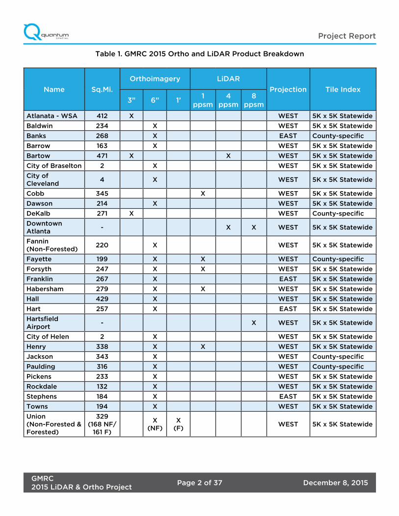
The delivered products conform to the specifications as stated in the Task Order and Quantum Spatial’s Technical Proposal. See Table 1 for more information.

1. Summary / Scope


Project Report

Table 1. GMRC 2015 Ortho and LiDAR Product Breakdown

Name Sq.Mi.

Orthoimagery LiDAR

Projection Tile Index

3” 6” 1’1

ppsm4

ppsm8

ppsm

Atlanata - WSA 412 X WEST 5K x 5K Statewide

Baldwin 234 X WEST 5K x 5K Statewide

Banks 268 X EAST County-specific

Barrow 163 X WEST 5K x 5K Statewide

Bartow 471 X X WEST 5K x 5K Statewide

City of Braselton 2 X WEST 5K x 5K Statewide

City of Cleveland

4 X WEST 5K x 5K Statewide

Cobb 345 X WEST 5K x 5K Statewide

Dawson 214 X WEST 5K x 5K Statewide

DeKalb 271 X WEST County-specific

Downtown Atlanta

- X X WEST 5K x 5K Statewide

Fannin(Non-Forested)

220 X WEST 5K x 5K Statewide

Fayette 199 X X WEST County-specific

Forsyth 247 X X WEST 5K x 5K Statewide

Franklin 267 X EAST 5K x 5K Statewide

Habersham 279 X X WEST 5K x 5K Statewide

Hall 429 X WEST 5K x 5K Statewide

Hart 257 X EAST 5K x 5K Statewide

Hartsfield Airport

- X WEST 5K x 5K Statewide

City of Helen 2 X WEST 5K x 5K Statewide

Henry 338 X X WEST 5K x 5K Statewide

Jackson 343 X WEST County-specific

Paulding 316 X WEST County-specific

Pickens 233 X WEST 5K x 5K Statewide

Rockdale 132 X WEST 5K x 5K Statewide

Stephens 184 X EAST 5K x 5K Statewide

Towns 194 X WEST 5K x 5K Statewide

Union(Non-Forested & Forested)

329(168 NF/

161 F)

X (NF)

X(F)

WEST 5K x 5K Statewide


Project Report

1.3. Location / Coverage

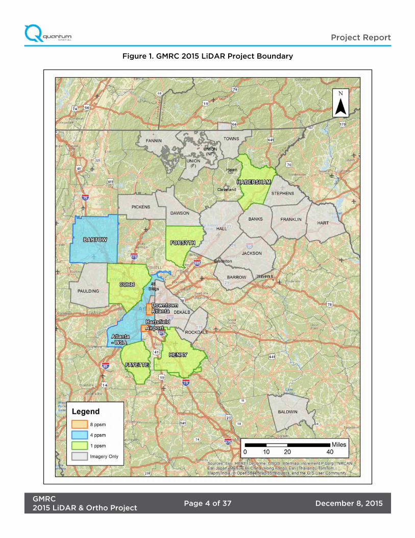
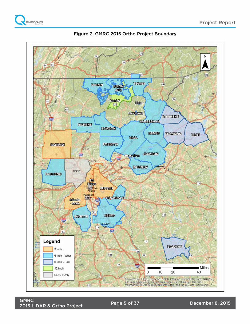
The GMRC 2015 LiDAR project boundary consists of 6 counties and 1 city. The project area is shown in Figure 1 on the following page. The Ortho project boundary includes 20 counties and 4 cities, as seen in Figure 2.

1.4.Duration

LiDAR missions were flown from January 18, 2015 through February 12, 2015 in 24 total lifts to complete coverage of the area. The imagery was acquired in 38 lifts from January 16, 2015 through April 9, 2015. See “Section: 2.6. Time Period” for more details.

1.5. Issues

Due to weather conditions, imagery acquisition was delayed, resulting in an actual imagery completion date of April 1, 2015 instead of the planned March 6, 2015. This pushed imagery production back and affected the overall imagery schedule.

1.6. Deliverables

The following products were produced and delivered:

Lidar• Unclassified raw point cloud swath LAS in version 1.2 format• Classified point cloud tiled LAS in version 1.2 format• DTM/TIN• Hydro-flattened DEM in ERDAS .IMG format• Hydro-flattened breaklines in Esri geodatabase format• 1-foot and 2-foot contours, in Esri shapefile format• Intensity images tiled in GeoTIFF format• Project level metadata

Ortho• 3” GeoTIFFs• 3” SIDs (Gen2 and Gen4)• 6” GeoTIFFs• 6” SIDs (Gen2 and Gen4)• 1’ GeoTIFFs• 1’ SIDs (Gen2 and Gen4)• Deliverable Level Metadata

Other• Planned and Actual flight line numbers and footprints in Esri shapefile format• GPS/IMU Report


Project Report

Figure 1. GMRC 2015 LiDAR Project Boundary


Project Report

Figure 2. GMRC 2015 Ortho Project Boundary


Project Report

2.1. Flight Planning Flight planning was based on the unique project requirements and characteristics of the project site. The basis of planning included: required accuracies, type of development, amount / type of vegetation within project area, required data posting, and potential altitude restrictions for flights in project vicinity.

Detailed project flight planning calculations were performed for the project using Leica Mission Pro planning software for LiDAR and imagery.

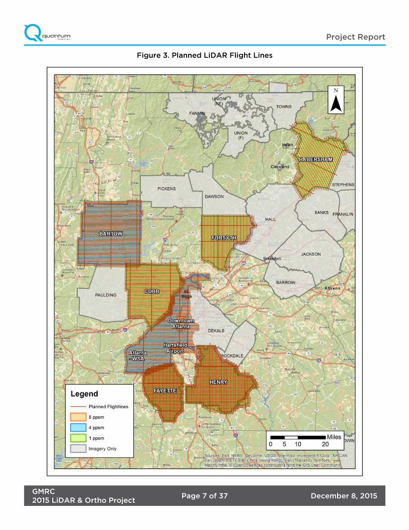
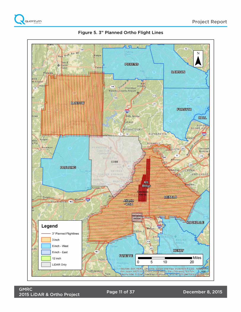
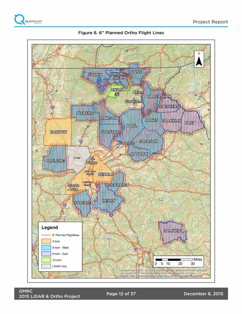
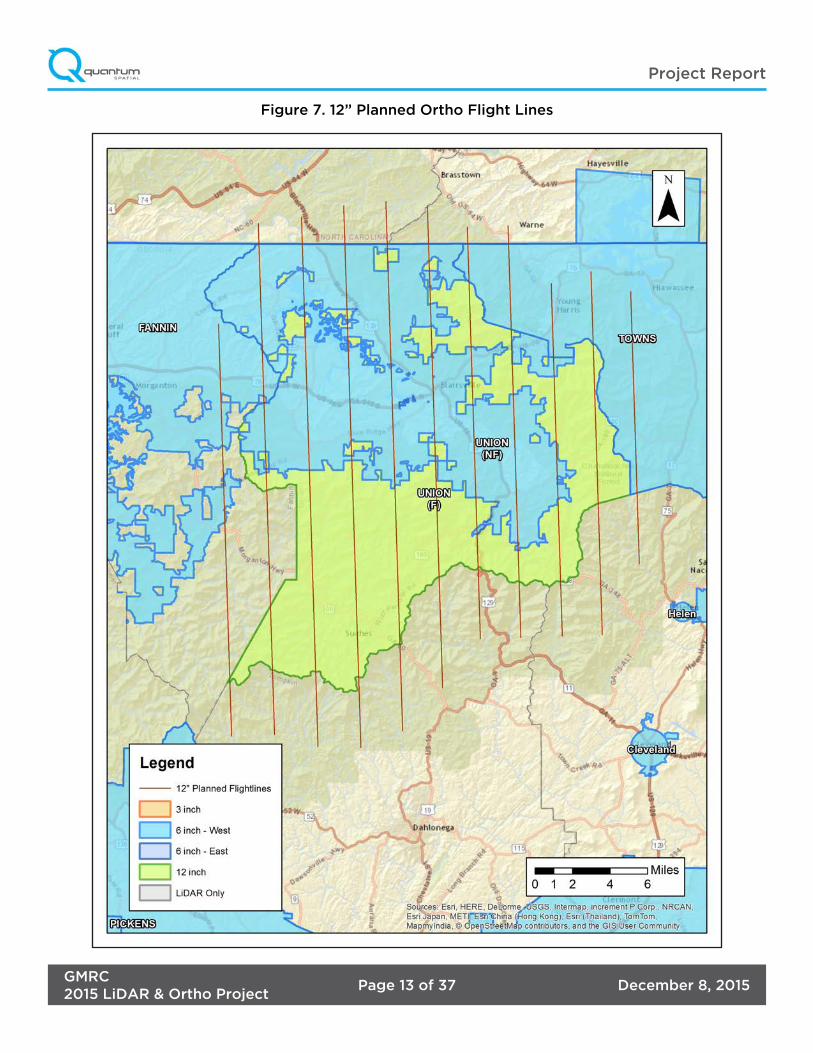
The entire target area was comprised of 710 planned flight lines and approximately total 11,946.16 flight line miles for LiDAR acquisition (Figure 3) and 457 planned flight lines for orthoimagery acquisition (Figure 5 - Figure 7).

2.2. LiDAR Sensor

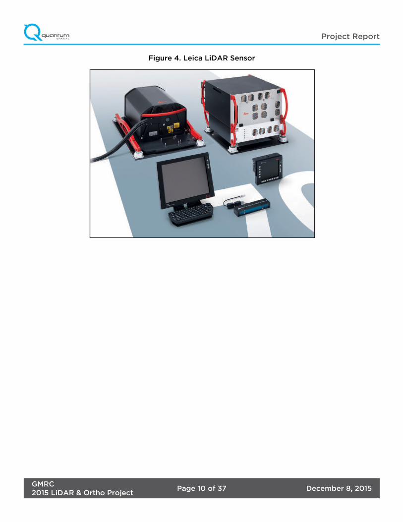
Quantum Spatial utilized a Leica ALS 70 LiDAR sensor (Figure 4), serial number 7161, during the project. The ALS 70 system is capable of collecting data at a maximum frequency of 500 kHz, which affords elevation data collection of up to 500,000 points per second. The system utilizes a Multi-Pulse in the Air option (MPIA). The sensor is also equipped with the ability to measure up to 4 returns per outgoing pulse from the laser and these come in the form of 1st, 2nd, 3rd and last returns. The intensity of the returns is also captured during aerial acquisition.

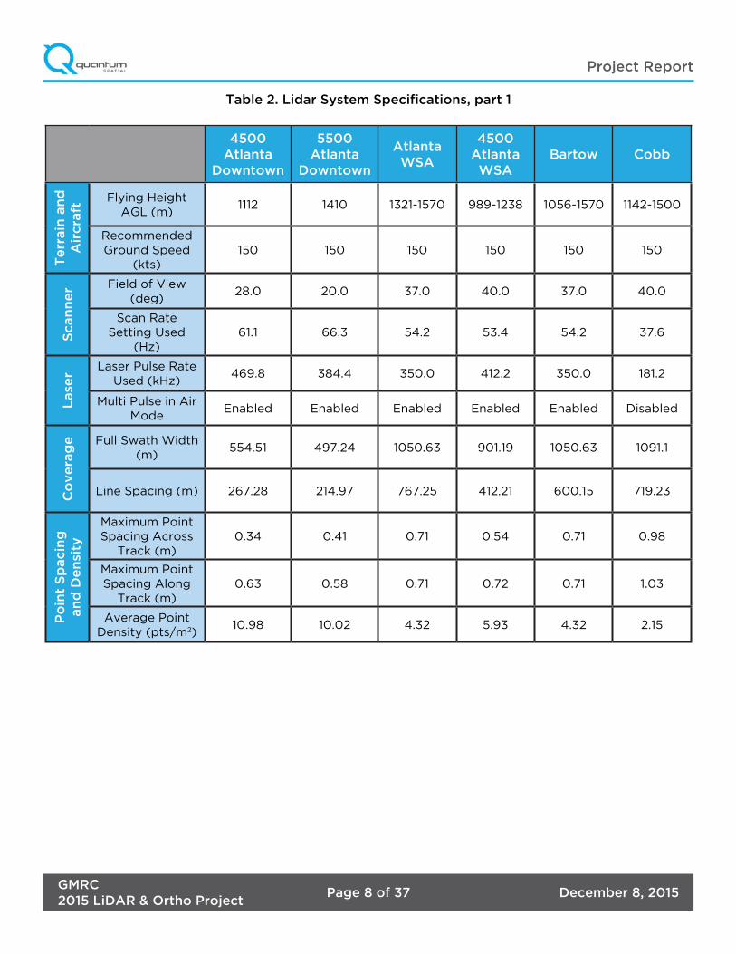
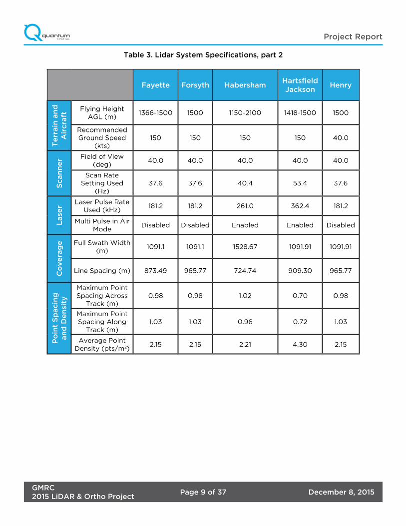
A brief summary of the aerial acquisition parameters for the project are shown in the LiDAR System Specifications in Table 2 and Table 3.

2.3. Orthoimagery Camera

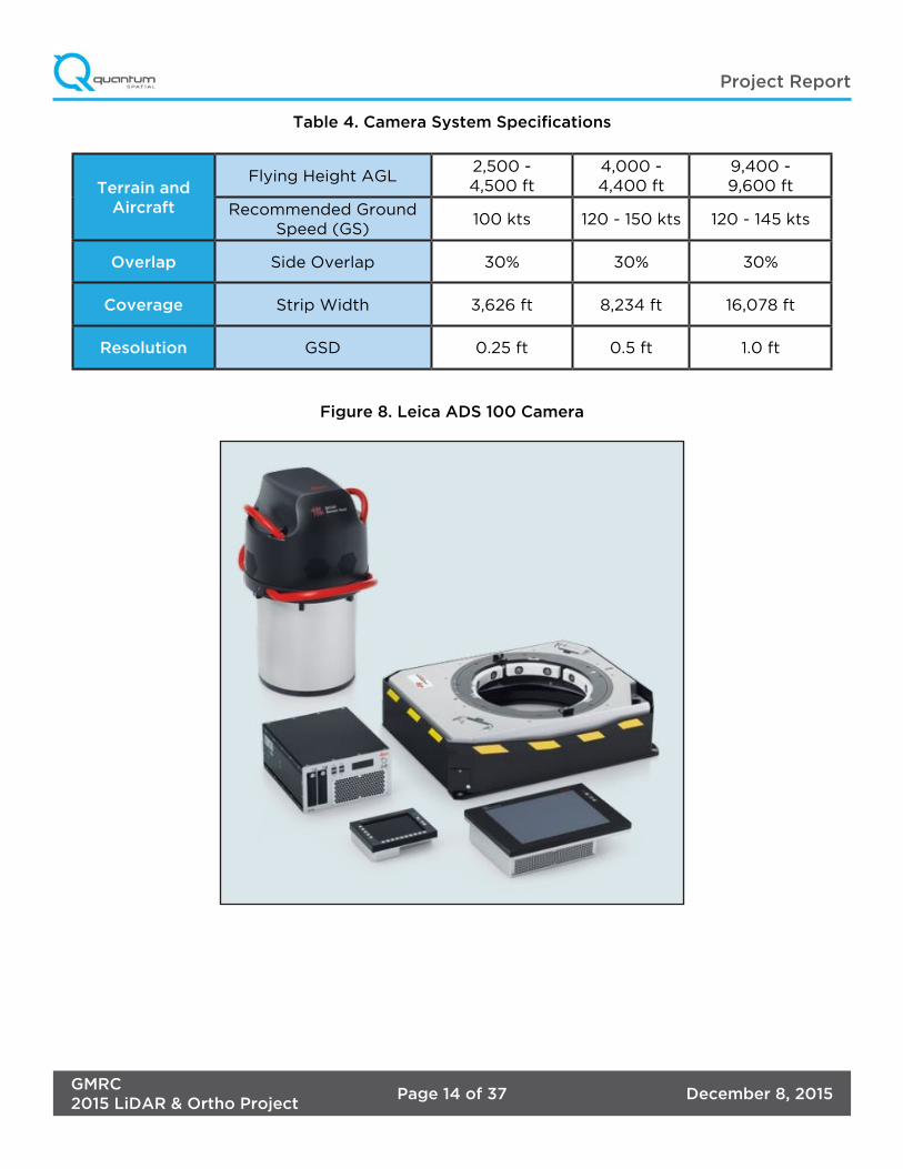
Quantum Spatial also utilized a Leica ADS 100 (Figure 8), serial number(s) 10541 and 10542. The system has 4 channel (RGB & NIR) multi-spectral capability with a strip width of 20,000 pixels. This system collects a constant “push-broom swath” of imagery. The Leica PAV100 gyro-stabilized mount with adaptive control insures the best possible image collection. This system utilizes a 62.5 mm lens focal distance.

A brief summary of the aerial acquisition parameters for the project are shown in the Camera System Specifications in Table 4.

2. Planning / Equipment


Project Report

Figure 3. Planned LiDAR Flight Lines


Project Report

Table 2. Lidar System Specifications, part 1

4500 Atlanta

Downtown

5500 Atlanta

Downtown

Atlanta WSA

4500 Atlanta WSA

Bartow Cobb

Te

rrain

an

d

Air

cra

ft

Flying Height AGL (m)

1112 1410 1321-1570 989-1238 1056-1570 1142-1500

Recommended Ground Speed

(kts)150 150 150 150 150 150

Scan

ne

r Field of View (deg)

28.0 20.0 37.0 40.0 37.0 40.0

Scan Rate Setting Used

(Hz)61.1 66.3 54.2 53.4 54.2 37.6

Lase

r

Laser Pulse Rate Used (kHz)

469.8 384.4 350.0 412.2 350.0 181.2

Multi Pulse in Air Mode

Enabled Enabled Enabled Enabled Enabled Disabled

Co

ve

rag

e Full Swath Width (m)

554.51 497.24 1050.63 901.19 1050.63 1091.1

Line Spacing (m) 267.28 214.97 767.25 412.21 600.15 719.23

Po

int

Sp

acin

g

an

d D

en

sity

Maximum Point Spacing Across

Track (m)0.34 0.41 0.71 0.54 0.71 0.98

Maximum Point Spacing Along

Track (m)0.63 0.58 0.71 0.72 0.71 1.03

Average Point Density (pts/m2)

10.98 10.02 4.32 5.93 4.32 2.15


Project Report

Table 3. Lidar System Specifications, part 2

Fayette Forsyth HabershamHartsfieldJackson

Henry

Te

rrain

an

d

Air

cra

ft

Flying Height AGL (m)

1366-1500 1500 1150-2100 1418-1500 1500

Recommended Ground Speed

(kts)150 150 150 150 40.0

Scan

ne

r Field of View (deg)

40.0 40.0 40.0 40.0 40.0

Scan Rate Setting Used

(Hz)37.6 37.6 40.4 53.4 37.6

Lase

r

Laser Pulse Rate Used (kHz)

181.2 181.2 261.0 362.4 181.2

Multi Pulse in Air Mode

Disabled Disabled Enabled Enabled Disabled

Co

ve

rag

e Full Swath Width (m)

1091.1 1091.1 1528.67 1091.91 1091.91

Line Spacing (m) 873.49 965.77 724.74 909.30 965.77

Po

int

Sp

acin

g

an

d D

en

sity

Maximum Point Spacing Across

Track (m)0.98 0.98 1.02 0.70 0.98

Maximum Point Spacing Along

Track (m)1.03 1.03 0.96 0.72 1.03

Average Point Density (pts/m2)

2.15 2.15 2.21 4.30 2.15


Project Report

Figure 4. Leica LiDAR Sensor


Project Report

Figure 5. 3” Planned Ortho Flight Lines


Project Report



Project Report



Project Report

Table 4. Camera System Specifications

Terrain and Aircraft

Flying Height AGL2,500 - 4,500 ft

4,000 - 4,400 ft

9,400 - 9,600 ft

Recommended Ground Speed (GS)

100 kts 120 - 150 kts 120 - 145 kts

Overlap Side Overlap 30% 30% 30%

Coverage Strip Width 3,626 ft 8,234 ft 16,078 ft

Resolution GSD 0.25 ft 0.5 ft 1.0 ft

Figure 8. Leica ADS 100 Camera


Project Report

2.4. Aircraft

All flights for the GMRC 2015 project were accomplished through the use of customized planes. Plane type and tail numbers are listed below.

LiDAR Collection Planes• Piper Navajo (twin-piston), Tail Numbers: N73TM and N812TB

Ortho Collection Planes• Cessna Conquest 2 (twin-turboprop), Tail Number: N441CJ• Cessna 206 Stationair (piston-sigle), Tail Number: N7266Z• Rockwell Turbo Commander 690 (twin-turboprop), Tail Numbers: N910FC, N690LN

These aircraft provided an ideal, stable aerial base for LiDAR and orthoimagery acquisition. These aerial platforms has relatively fast cruise speeds which are beneficial for project mobilization / demobilization while maintaining relatively slow stall speeds which proved ideal for collection of high-density, consistent data posting using state-of-the-art Leica LiDAR and imagery systems. Some of the operating aircraft can be seen in Figure 9 below.

Figure 9. Some of Quantum Spatial’s Planes


Project Report

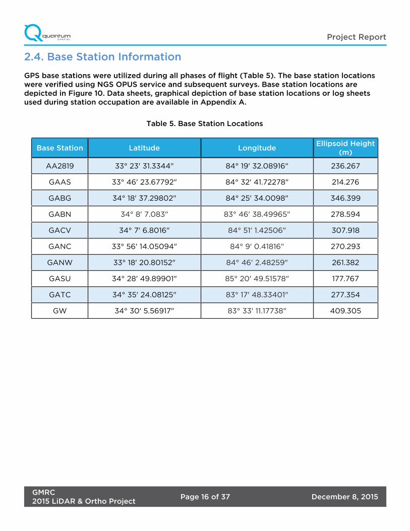
Table 5. Base Station Locations

Base Station Latitude LongitudeEllipsoid Height

(m)

AA2819 33° 23' 31.3344" 84° 19' 32.08916" 236.267

GAAS 33° 46' 23.67792" 84° 32' 41.72278" 214.276

GABG 34° 18' 37.29802" 84° 25' 34.0098" 346.399

GABN 34° 8' 7.083" 83° 46' 38.49965" 278.594

GACV 34° 7' 6.8016" 84° 51' 1.42506" 307.918

GANC 33° 56' 14.05094" 84° 9' 0.41816" 270.293

GANW 33° 18' 20.80152" 84° 46' 2.48259" 261.382

GASU 34° 28' 49.89901" 85° 20' 49.51578" 177.767

GATC 34° 35' 24.08125" 83° 17' 48.33401" 277.354

GW 34° 30' 5.56917" 83° 33' 11.17738" 409.305

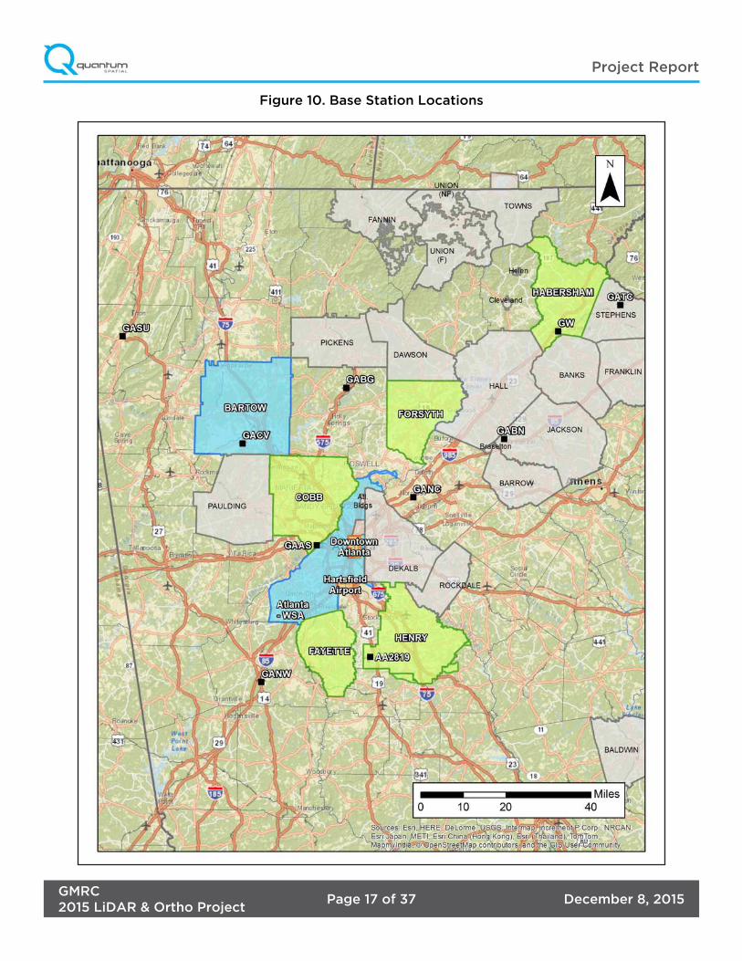
2.4. Base Station Information

GPS base stations were utilized during all phases of flight (Table 5). The base station locations were verified using NGS OPUS service and subsequent surveys. Base station locations are depicted in Figure 10. Data sheets, graphical depiction of base station locations or log sheets used during station occupation are available in Appendix A.


Project Report

Figure 10. Base Station Locations


Project Report

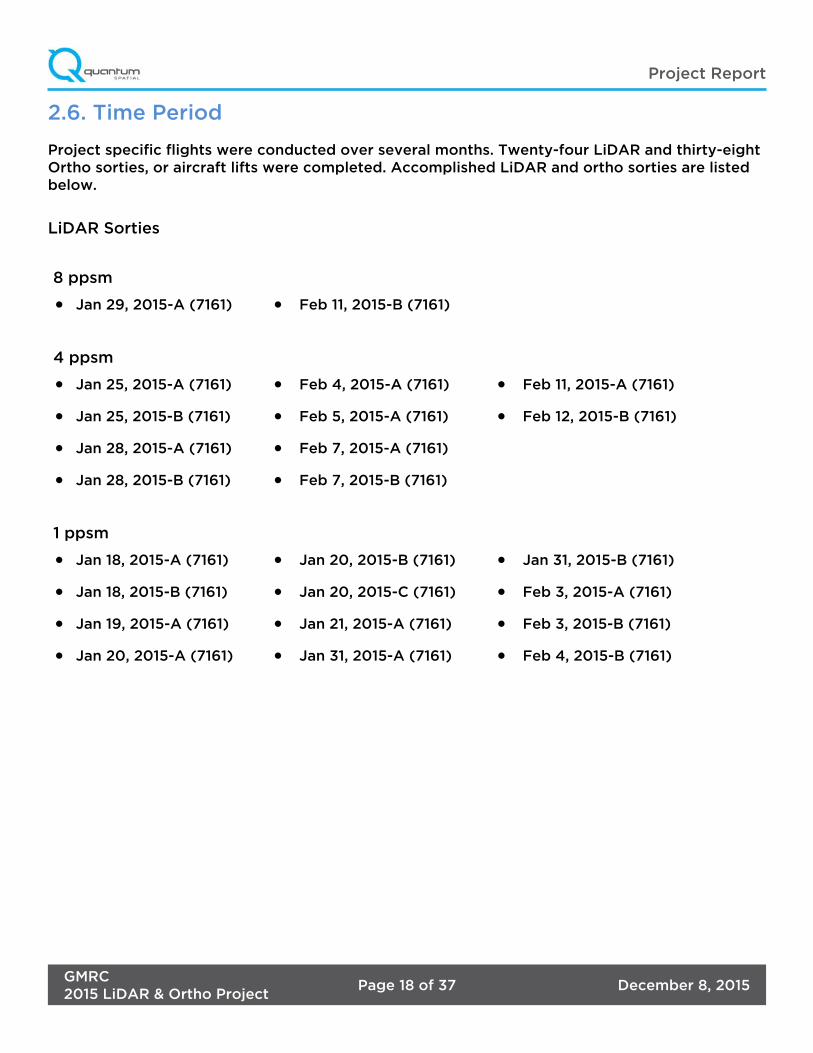
LiDAR Sorties

8 ppsm

• Jan 29, 2015-A (7161) • Feb 11, 2015-B (7161)

4 ppsm

• Jan 25, 2015-A (7161) • Feb 4, 2015-A (7161) • Feb 11, 2015-A (7161)

• Jan 25, 2015-B (7161) • Feb 5, 2015-A (7161) • Feb 12, 2015-B (7161)

• Jan 28, 2015-A (7161) • Feb 7, 2015-A (7161)

• Jan 28, 2015-B (7161) • Feb 7, 2015-B (7161)

1 ppsm

• Jan 18, 2015-A (7161) • Jan 20, 2015-B (7161) • Jan 31, 2015-B (7161)

• Jan 18, 2015-B (7161) • Jan 20, 2015-C (7161) • Feb 3, 2015-A (7161)

• Jan 19, 2015-A (7161) • Jan 21, 2015-A (7161) • Feb 3, 2015-B (7161)

• Jan 20, 2015-A (7161) • Jan 31, 2015-A (7161) • Feb 4, 2015-B (7161)

2.6. Time Period

Project specific flights were conducted over several months. Twenty-four LiDAR and thirty-eight Ortho sorties, or aircraft lifts were completed. Accomplished LiDAR and ortho sorties are listed below.


Project Report

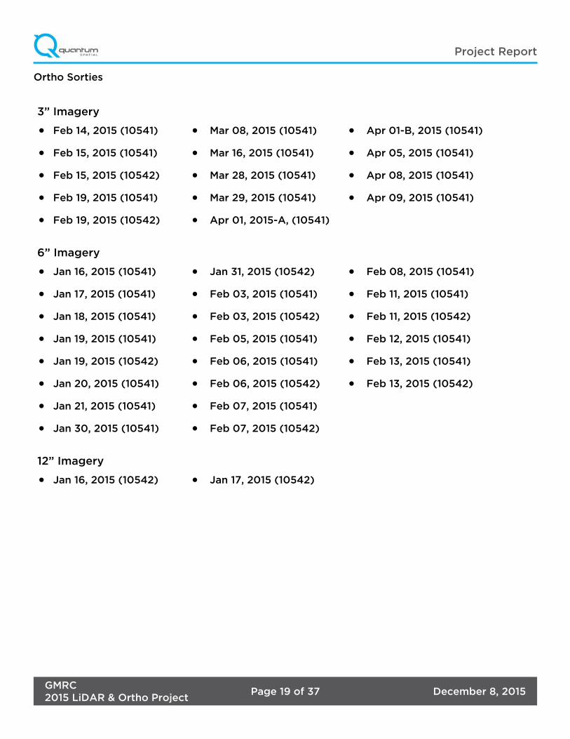
Ortho Sorties

3” Imagery

• Feb 14, 2015 (10541) • Mar 08, 2015 (10541) • Apr 01-B, 2015 (10541)

• Feb 15, 2015 (10541) • Mar 16, 2015 (10541) • Apr 05, 2015 (10541)

• Feb 15, 2015 (10542) • Mar 28, 2015 (10541) • Apr 08, 2015 (10541)

• Feb 19, 2015 (10541) • Mar 29, 2015 (10541) • Apr 09, 2015 (10541)

• Feb 19, 2015 (10542) • Apr 01, 2015-A, (10541)

6” Imagery

• Jan 16, 2015 (10541) • Jan 31, 2015 (10542) • Feb 08, 2015 (10541)

• Jan 17, 2015 (10541) • Feb 03, 2015 (10541) • Feb 11, 2015 (10541)

• Jan 18, 2015 (10541) • Feb 03, 2015 (10542) • Feb 11, 2015 (10542)

• Jan 19, 2015 (10541) • Feb 05, 2015 (10541) • Feb 12, 2015 (10541)

• Jan 19, 2015 (10542) • Feb 06, 2015 (10541) • Feb 13, 2015 (10541)

• Jan 20, 2015 (10541) • Feb 06, 2015 (10542) • Feb 13, 2015 (10542)

• Jan 21, 2015 (10541) • Feb 07, 2015 (10541)

• Jan 30, 2015 (10541) • Feb 07, 2015 (10542)

12” Imagery

• Jan 16, 2015 (10542) • Jan 17, 2015 (10542)


Project Report

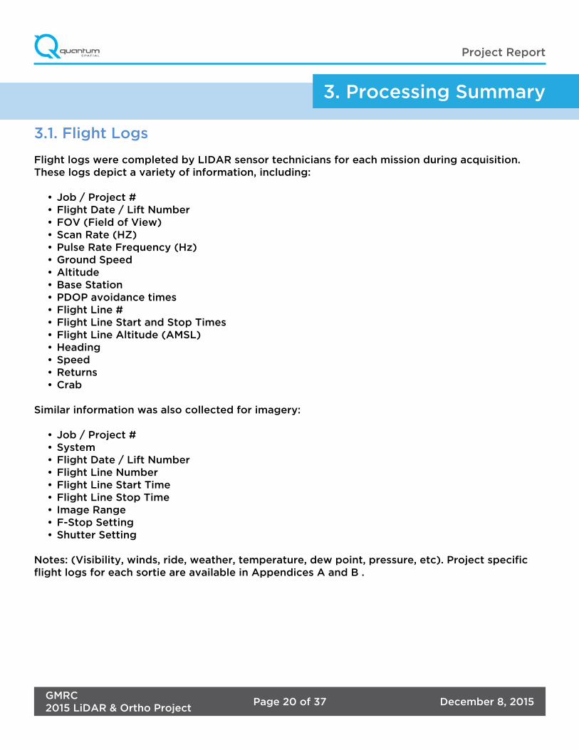
3.1. Flight Logs

Flight logs were completed by LIDAR sensor technicians for each mission during acquisition. These logs depict a variety of information, including:

• Job / Project #• Flight Date / Lift Number• FOV (Field of View) • Scan Rate (HZ) • Pulse Rate Frequency (Hz)• Ground Speed• Altitude• Base Station• PDOP avoidance times• Flight Line #• Flight Line Start and Stop Times• Flight Line Altitude (AMSL)• Heading• Speed• Returns• Crab

Similar information was also collected for imagery:

• Job / Project #• System• Flight Date / Lift Number• Flight Line Number• Flight Line Start Time• Flight Line Stop Time• Image Range• F-Stop Setting• Shutter Setting

Notes: (Visibility, winds, ride, weather, temperature, dew point, pressure, etc). Project specific flight logs for each sortie are available in Appendices A and B .

3. Processing Summary


Project Report

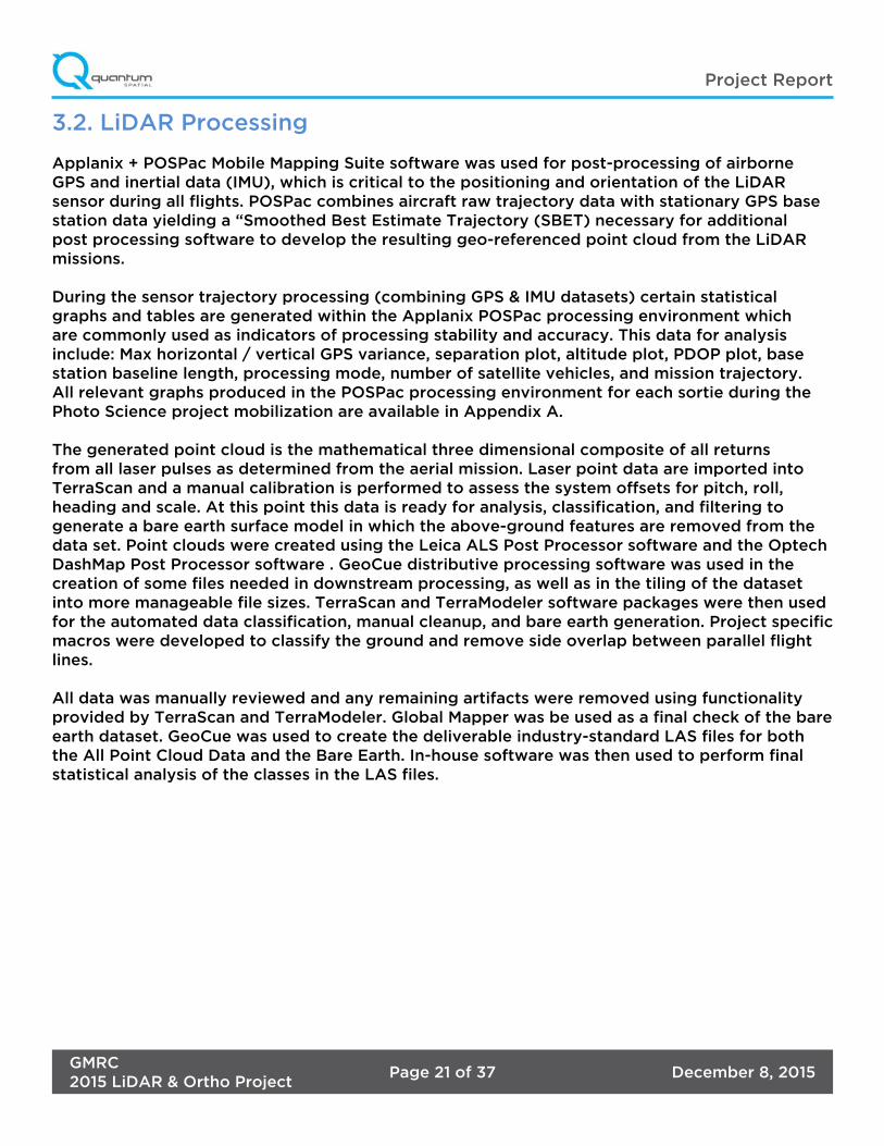
3.2. LiDAR Processing

Applanix + POSPac Mobile Mapping Suite software was used for post-processing of airborne GPS and inertial data (IMU), which is critical to the positioning and orientation of the LiDAR sensor during all flights. POSPac combines aircraft raw trajectory data with stationary GPS base station data yielding a “Smoothed Best Estimate Trajectory (SBET) necessary for additional post processing software to develop the resulting geo-referenced point cloud from the LiDAR missions.

During the sensor trajectory processing (combining GPS & IMU datasets) certain statistical graphs and tables are generated within the Applanix POSPac processing environment which are commonly used as indicators of processing stability and accuracy. This data for analysis include: Max horizontal / vertical GPS variance, separation plot, altitude plot, PDOP plot, base station baseline length, processing mode, number of satellite vehicles, and mission trajectory. All relevant graphs produced in the POSPac processing environment for each sortie during the Photo Science project mobilization are available in Appendix A.

The generated point cloud is the mathematical three dimensional composite of all returns from all laser pulses as determined from the aerial mission. Laser point data are imported into TerraScan and a manual calibration is performed to assess the system offsets for pitch, roll, heading and scale. At this point this data is ready for analysis, classification, and filtering to generate a bare earth surface model in which the above-ground features are removed from the data set. Point clouds were created using the Leica ALS Post Processor software and the Optech DashMap Post Processor software . GeoCue distributive processing software was used in the creation of some files needed in downstream processing, as well as in the tiling of the dataset into more manageable file sizes. TerraScan and TerraModeler software packages were then used for the automated data classification, manual cleanup, and bare earth generation. Project specific macros were developed to classify the ground and remove side overlap between parallel flight lines.

All data was manually reviewed and any remaining artifacts were removed using functionality provided by TerraScan and TerraModeler. Global Mapper was be used as a final check of the bare earth dataset. GeoCue was used to create the deliverable industry-standard LAS files for both the All Point Cloud Data and the Bare Earth. In-house software was then used to perform final statistical analysis of the classes in the LAS files.


Project Report

3.3. LAS Classification Scheme

The classification classes are determined by the USGS Version 1.0 specifications and are an industry standard for the classification of LIDAR point clouds. All data starts the process as Class 1 (Unclassified), and then through automated classification routines, the classifications are determined using TerraScan macro processing.

The classes used in the dataset are as follows and have the following descriptions:

• Class 1 – Processed, but Unclassified – These points would be the catch all for points that do not fit any of the other deliverable classes. This would cover features such as vegetation, cars, etc.

• Class 2 – Bare earth ground – This is the bare earth surface• Class 3 – Low Vegetation• Class 4 – Medium Vegetation• Class 5 – High Vegetation• Class 6 – Buildings• Class 7 – Low Points – Low points, manually identified above or below the surface that could

be noise points in point cloud.• Class 9 – In-land Water – Points found inside of inland lake/ponds• Class 10 – Ignored Ground – Points found to be close to breakline features. Points are moved

to this class from the Class 2 dataset. This class is ignored during the DEM creation process in order to provide smooth transition between the ground surface and hydro flattened surface.

• Class 17 (Atlanta only) – Bridge Decks – Points falling on bridge decks.• Class 17 (All other datasets) – Overlap Default (Unclassified) – Points found in the overlap

between flight lines. These points are created through automated processing methods and not cleaned up during processing.

• Class 18 – Overlap Bare-earth ground – Points found in the overlap between flight lines. These points are created through automated processing, matching the specifications determined during the automated process, that are close to the Class 2 dataset (when analyzed using height from ground analysis)

• Class 25 – Overlap Water – Points found in the overlap between flight lines that are located inside hydro features. These points are created through automated processing methods and not cleaned up during processing.

3.4. Classified LAS Processing

The bare earth surface is then manually reviewed to ensure correct classification on the Class 2 (Ground) points. After the bare- earth surface is finalized; it is then used to generate all hydro-breaklines through heads-up digitization.

All ground (ASPRS Class 2) LiDAR data inside of the Lake Pond and Double Line Drain hydro flattening breaklines were then classified to water (ASPRS Class 9) using TerraScan macro functionality. A buffer of 3 feet was also used around each hydro flattened feature to classify these ground (ASPRS Class 2) points to Ignored ground (ASPRS Class 10). All Lake Pond Island and Double Line Drain Island features were checked to ensure that the ground (ASPRS Class


Project Report

2) points were reclassified to the correct classification after the automated classification was completed.

All overlap data was processed through automated functionality provided by TerraScan to classify the overlapping flight line data to approved classes by USGS. The overlap data was classified to Class 17 (Overlap Default) and Class 18 (Overlap Ground). These classes were created through automated processes only and were not verified for classification accuracy. Due to software limitations within TerraScan, these classes were used to trip the withheld bit within various software packages. These processes were reviewed and accepted by USGS through numerous conference calls and pilot study areas.

All data was manually reviewed and any remaining artifacts removed using functionality provided by TerraScan and TerraModeler. Global Mapper is used as a final check of the bare earth dataset. GeoCue was then used to create the deliverable industry-standard LAS files for all point cloud data. Quantum Spatial proprietary software was used to perform final statistical analysis of the classes in the LAS files, on a per tile level to verify final classification metrics and full LAS header information.

3.5. Hydro-Flattening Breakline Process

Class 2 LiDAR was used to create a bare earth surface model. The surface model was then used to heads-up digitize 2D breaklines of Inland Streams and Rivers with a 100 foot nominal width and Inland Ponds and Lakes of 2 acres or greater surface area.

Elevation values were assigned to all Inland Ponds and Lakes, Inland Pond and Lake Islands, Inland Streams and Rivers and Inland Stream and River Islands using TerraModeler functionality.

Elevation values were assigned to all Inland streams and rivers using Photo Science proprietary software.

All ground (ASPRS Class 2) LiDAR data inside of the collected inland breaklines were then classified to water (ASPRS Class 9) using TerraScan macro functionality. A buffer of 3 feet was also used around each hydro flattened feature. These points were moved from ground (ASPRS Class 2) to Ignored Ground (ASPRS Class 10).

The breakline files were then translated to ESRI Shapefile format using ESRI conversion tools.

3.6. Hydro-Flattening Raster DEM Process

Class 2 LiDAR in conjunction with the hydro breaklines were used to create Raster Digital Elevation Models. Using automated scripting routines within ArcMap, an ERDAS Imagine IMG file was created for each tile. Each surface is reviewed using Global Mapper to check for any surface anomalies or incorrect elevations found within the surface.


Project Report

3.7. Imagery Processing Summary

There are several distinct processing steps. First, raw imagery is converted from the raw data collected in flight and post-processed to a “RAW” file that can be incorporated into orthophotography data. Next, Ground Control Points (GCPs) were collected and processed. Then, an additional set of raw data collected in flight from the Airborne GPS systems are processed to create an external orientation file. The processed RAW imagery, ground control and the external orientation file are used to create aerotriangulation data. Finally, the merging of all of these, along with a surface, is done in order to create a digital orthophotograph.

3.8. Raw Data Extraction

Leica Geosystems XPro version 6.2.1 was used to download the raw flight data from the MMU. Raw data for the ADS sensor consists of the un-rectified strip images in TIFF format, commonly referred to as L0 images in ADS workflows, and the raw ABGPS/IMU observables.

3.9. ABGPS / IMU

ABGPS/IMU data was collected on the aircraft during the survey mission, providing sensor position and orientation information for geo-referencing the imagery data. ABGPS observations were collected at a frequency of 2Hz, and IMU observations were collected at a frequency of 200Hz. Precise lever arm measurements from the ABGPS/IMU measurement reference points to the principal point of the ADS focal plane are used in reducing the raw vehicle position/attitude observables to sensor exterior orientation. These lever arm measurements are measured during sensor installation in the survey aircraft.

GPS data was collected using base stations, providing corrections to support differential post-processing of the ABGPS. More information can be found in Appendix B. Differential correction of the ABGPS data using the ground base station data was performed in NovAtel Inertial Explorer software version 8.6. The NAD83(2011) geodetic coordinates acquired through the CORS network were held as reference during differential correction. Corrected ABGPS data was combined with IMU data in Inertial Explorer through a Kalman filtering algorithm to arrive at a smoothed best estimate of the sensor’s trajectory during the collection missions. This trajectory estimate along with precise exposure timing data provide initial EO estimates for the imagery in aero-triangulation.

3.10. Aerotriangulation

Aero-triangulation was performed using Leica Geosystems’ XPro software version 6.2.1. XPro’s automatic point matching algorithm was used to match image tie points in the side overlap between adjacent image strips. The tie point observations were used in a least squares bundle adjustment to solve for systematic errors in the smoothed best estimate of trajectory, including GPS drift and timing offsets. The bundle adjustment also identifies and eliminates measurement blunders in the tie points.


Project Report

After solving for systematic navigation errors and removing measurement blunders, ground control points were manually measured in the imagery. Ground control points coordinates used had horizontal reference of Georgia State Plane West or East, NAD83(2011), US feet; and vertical reference of NAVD88 ellipsoid heights, US feet. AT for the ADS sensor is performed in the ellipsoid vertical reference to avoid systematic errors that geoid undulations cause in the pushbroom sensor model. The ground control point observations are used to solve for any remaining datum transformation required to determine EO in the project datum. Ground control points were assigned statistical weight, equivalent to their estimated accuracy, in the final least squares adjustment to solve for the control datum transformation.

3.11 Surface Model

Quantum Spatial generated an elevation model by combining newly collect LiDAR, client-provided surfaces, and data from the National Elevation Dataset.

3.12. Orthorectification

Orthorectification of imagery was accomplished with the XPro software version 6.2.1 rectification module, which provided a seamless workflow for block bundle adjustment and generation of orthoimages. The XPro rectification module used the block bundle adjustment solution developed in the bundle adjustment module and the L0 images as inputs.

Radiometric correction of the imagery included applying the manufacturer’s calibration and a proprietary process to account for atmospheric and lighting effects. Two principal effects were considered in the proprietary correction; atmospheric haze and bi-directional reflectance. Atmospheric haze describes the effect of sunlight reflecting off of aerosols dispersed in the atmosphere, especially in the blue wavelength of the visible light spectrum. Bi-directional reflectance describes the non-uniform brightness of the ground scene in an aerial image caused by varied viewing and illumination angles. Due to the ADS sensor’s consistent nadir geometry in the along-track flight direction of the image strip, haze and reflectance only affect the ADS sensor in the across track direction of the image strip. The algorithm works by sampling the pixel values throughout the image strip and calculating an average pixel value for each column of pixels across the sensor track. A polynomial function is used to normalize the samples to remove any anomalies, such as specular reflection on water, from the column averages. Mean brightness of the column averages are calculated, and a correction value determined to adjust the average pixel value of each column in the strip to the mean. The corrections were calculated and applied in the raw 12-bit dynamic range of the ADS sensor, permitting a more accurate correction than one applied after the imagery has been histogram stretched for 8-bit storage and viewing. Correction values were stored in separate files for each multi-spectral image and were applied by the orthorectification module during orthoimage output. The manufacturer’s factory calibrated radiometric gain parameters were also applied during orthorectification, modeling the variable sensitivity of each CCD in the ADS sensor to the wavelength of light it is assigned to collect.

The assembled DEM and atmospheric correction files were added to the XPro block definition. The rectification module was used to generate a 4-band orthorectified image strip, commonly referred to as L2 images in ADS workflows. The band order of the L2 was Red in Band 1, Green


Project Report

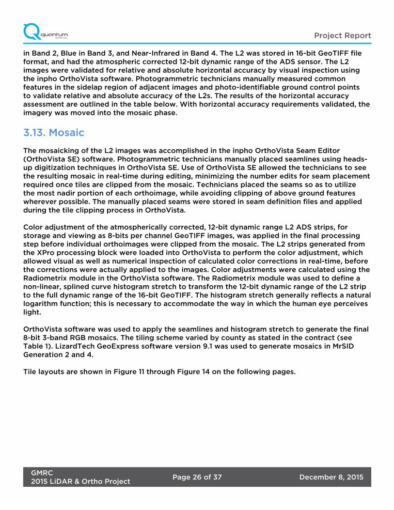
in Band 2, Blue in Band 3, and Near-Infrared in Band 4. The L2 was stored in 16-bit GeoTIFF file format, and had the atmospheric corrected 12-bit dynamic range of the ADS sensor. The L2 images were validated for relative and absolute horizontal accuracy by visual inspection using the inpho OrthoVista software. Photogrammetric technicians manually measured common features in the sidelap region of adjacent images and photo-identifiable ground control points to validate relative and absolute accuracy of the L2s. The results of the horizontal accuracy assessment are outlined in the table below. With horizontal accuracy requirements validated, the imagery was moved into the mosaic phase.

3.13. Mosaic

The mosaicking of the L2 images was accomplished in the inpho OrthoVista Seam Editor (OrthoVista SE) software. Photogrammetric technicians manually placed seamlines using heads-up digitization techniques in OrthoVista SE. Use of OrthoVista SE allowed the technicians to see the resulting mosaic in real-time during editing, minimizing the number edits for seam placement required once tiles are clipped from the mosaic. Technicians placed the seams so as to utilize the most nadir portion of each orthoimage, while avoiding clipping of above ground features wherever possible. The manually placed seams were stored in seam definition files and applied during the tile clipping process in OrthoVista.

Color adjustment of the atmospherically corrected, 12-bit dynamic range L2 ADS strips, for storage and viewing as 8-bits per channel GeoTIFF images, was applied in the final processing step before individual orthoimages were clipped from the mosaic. The L2 strips generated from the XPro processing block were loaded into OrthoVista to perform the color adjustment, which allowed visual as well as numerical inspection of calculated color corrections in real-time, before the corrections were actually applied to the images. Color adjustments were calculated using the Radiometrix module in the OrthoVista software. The Radiometrix module was used to define a non-linear, splined curve histogram stretch to transform the 12-bit dynamic range of the L2 strip to the full dynamic range of the 16-bit GeoTIFF. The histogram stretch generally reflects a natural logarithm function; this is necessary to accommodate the way in which the human eye perceives light.

OrthoVista software was used to apply the seamlines and histogram stretch to generate the final 8-bit 3-band RGB mosaics. The tiling scheme varied by county as stated in the contract (see Table 1). LizardTech GeoExpress software version 9.1 was used to generate mosaics in MrSID Generation 2 and 4.

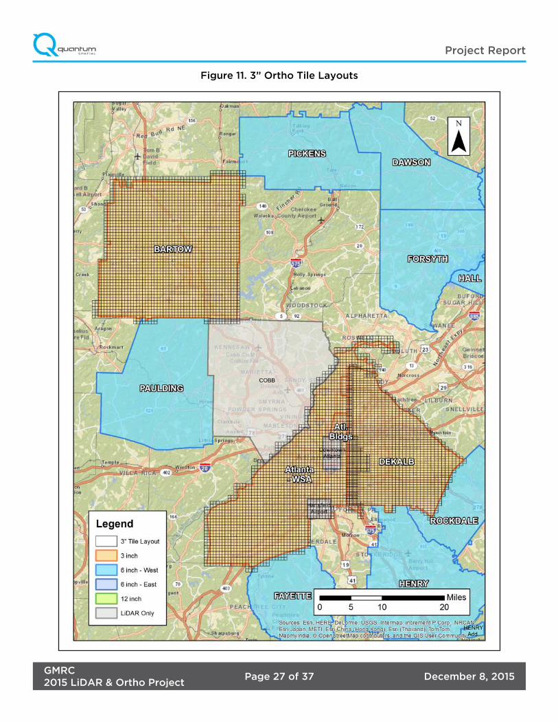
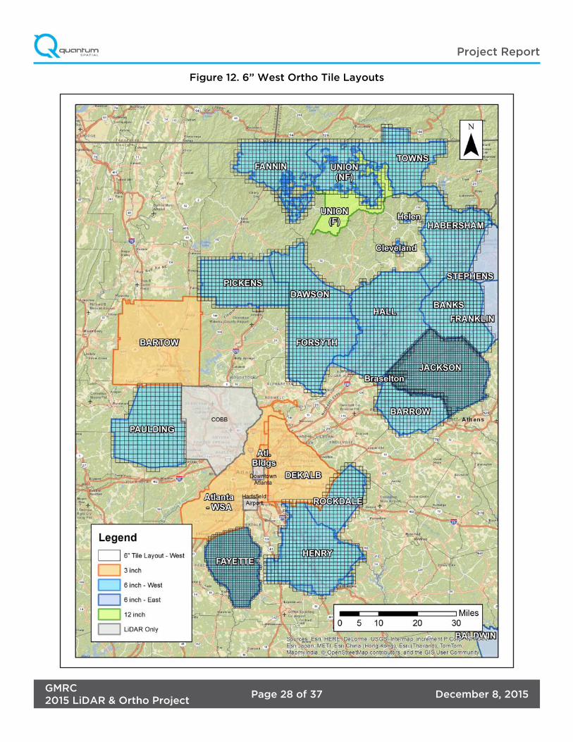
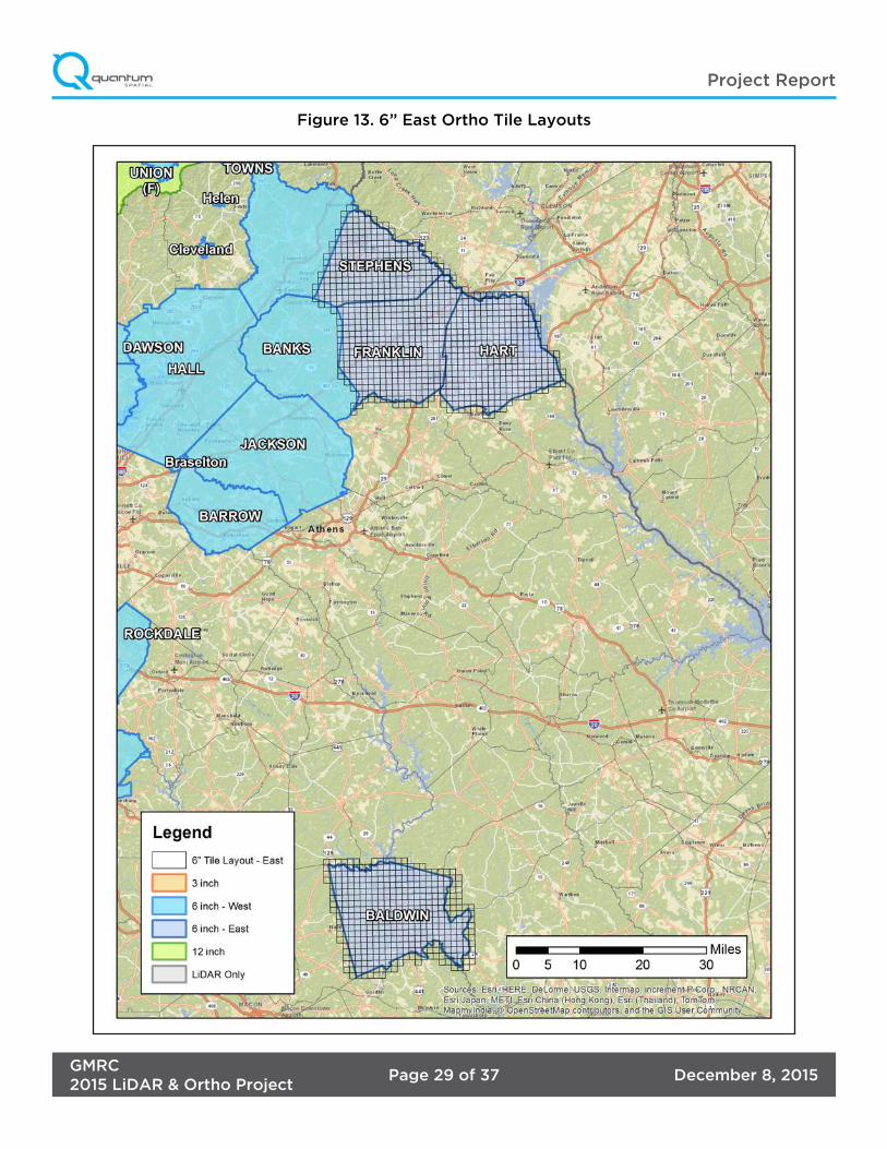
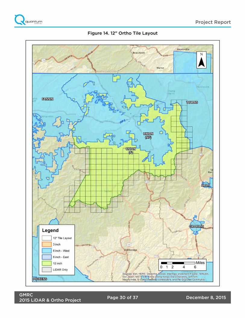
Tile layouts are shown in Figure 11 through Figure 14 on the following pages.


Project Report

Figure 11. 3” Ortho Tile Layouts


Project Report

Figure 12. 6” West Ortho Tile Layouts


Project Report

Figure 13. 6” East Ortho Tile Layouts


Project Report

Figure 14. 12” Ortho Tile Layout


Project Report

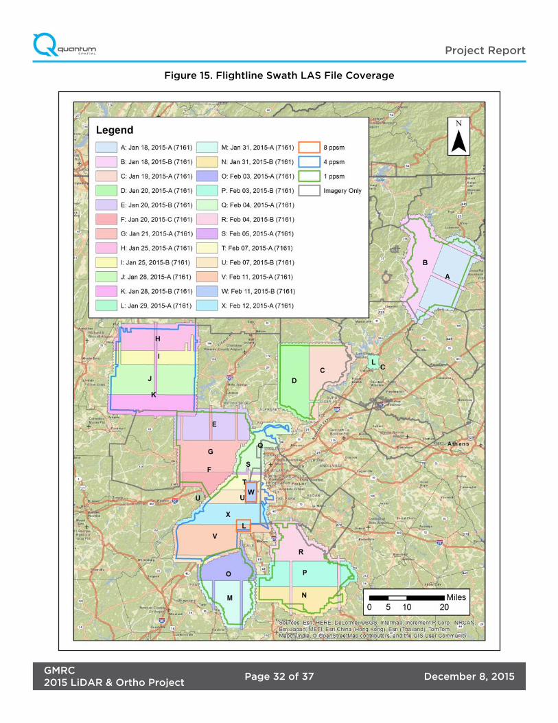
Coverage verification was performed by comparing coverage of processed .LAS files captured during project collection to generate project shape files depicting boundaries of specified project areas. Please refer to Figure 15.

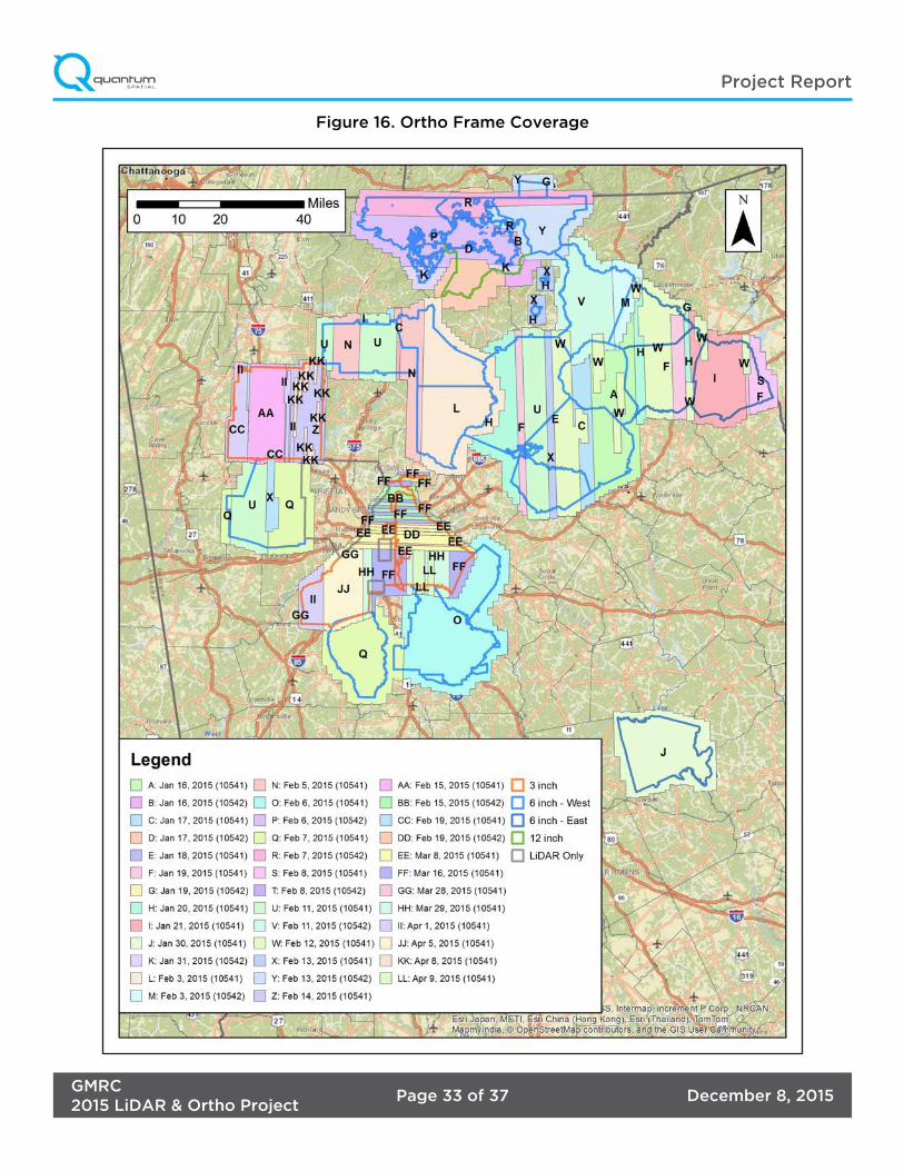
Imagery frame coverage (see Figure 16) and content verification was performed and validated by visual review. This action was performed in the field by flight crew during the acquisition phase as well as by imagery QA technicians at our processing center. The ABGPS/IMU and base station data was uploaded to the company FTP site after each flight for the INS processing team in Lexington, Kentucky to verify accuracy of data collected.

4. Project Coverage Verification


Project Report

Figure 15. Flightline Swath LAS File Coverage


Project Report

Figure 16. Ortho Frame Coverage


Project Report

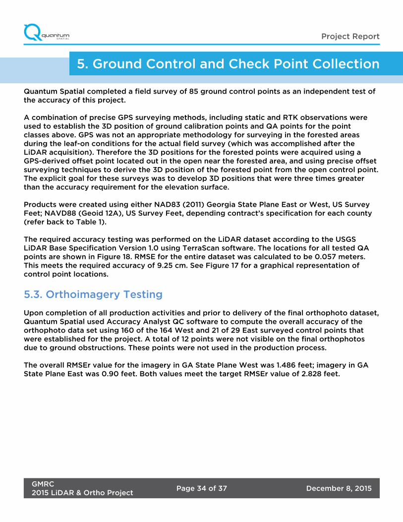
Quantum Spatial completed a field survey of 85 ground control points as an independent test of the accuracy of this project.

A combination of precise GPS surveying methods, including static and RTK observations were used to establish the 3D position of ground calibration points and QA points for the point classes above. GPS was not an appropriate methodology for surveying in the forested areas during the leaf-on conditions for the actual field survey (which was accomplished after the LiDAR acquisition). Therefore the 3D positions for the forested points were acquired using a GPS-derived offset point located out in the open near the forested area, and using precise offset surveying techniques to derive the 3D position of the forested point from the open control point. The explicit goal for these surveys was to develop 3D positions that were three times greater than the accuracy requirement for the elevation surface.

Products were created using either NAD83 (2011) Georgia State Plane East or West, US Survey Feet; NAVD88 (Geoid 12A), US Survey Feet, depending contract’s specification for each county (refer back to Table 1).

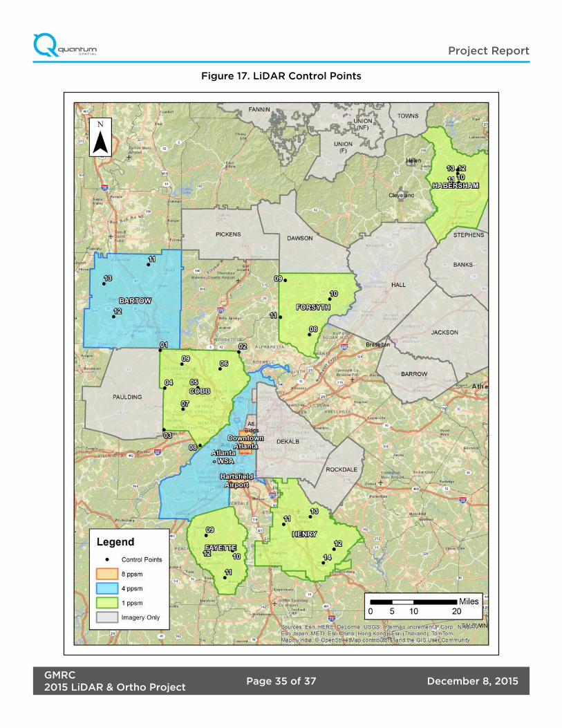
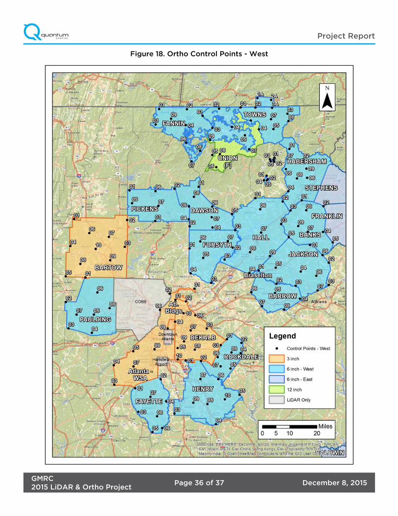
The required accuracy testing was performed on the LiDAR dataset according to the USGS LiDAR Base Specification Version 1.0 using TerraScan software. The locations for all tested QA points are shown in Figure 18. RMSE for the entire dataset was calculated to be 0.057 meters. This meets the required accuracy of 9.25 cm. See Figure 17 for a graphical representation of control point locations.

5.3. Orthoimagery Testing

Upon completion of all production activities and prior to delivery of the final orthophoto dataset, Quantum Spatial used Accuracy Analyst QC software to compute the overall accuracy of the orthophoto data set using 160 of the 164 West and 21 of 29 East surveyed control points that were established for the project. A total of 12 points were not visible on the final orthophotos due to ground obstructions. These points were not used in the production process.

The overall RMSEr value for the imagery in GA State Plane West was 1.486 feet; imagery in GA State Plane East was 0.90 feet. Both values meet the target RMSEr value of 2.828 feet.

5. Ground Control and Check Point Collection


Project Report

Figure 17. LiDAR Control Points


Project Report

Figure 18. Ortho Control Points - West


Project Report

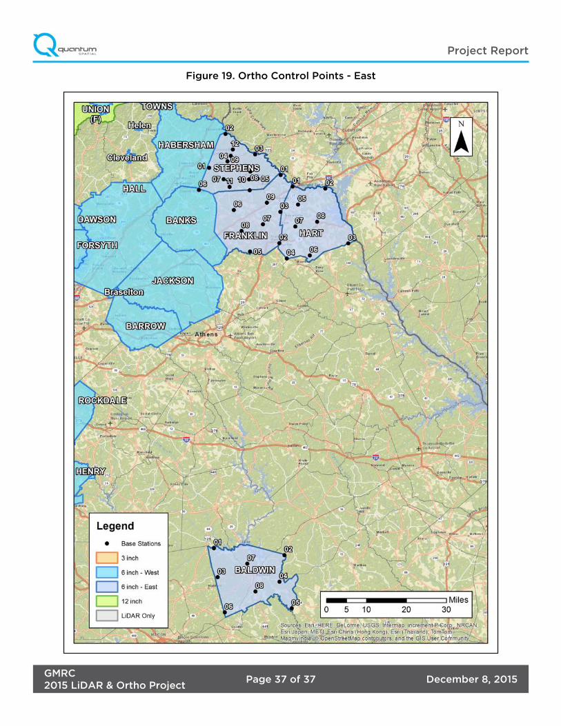
Figure 19. Ortho Control Points - East

Documents

GMRC 2015 LiDAR and Orthoimagery Project December 8, 2015 Quantum Spatial, Inc. 523 Wellington Way, Suite 375 Lexington, KY 40503. 859-277-8700 Prepared by: GMRC 2015 LiDAR and Orthoimagery