GEOTECHNICAL ENGINEERING – II

Subject Code : 06CV54 Internal Assessment Marks : 25

PART A

UNIT 3

CLASSIFICATION OF SOILS: Purpose of soil classification, basis for soil classification,

Particle size classification – MIT classification and IS classification, Textural

classification. Unified soil classification and IS classification - Plasticity chart and its

importance, Field identification of soils.

CLAY MIERALOGY AND SOIL STUCTURE: Single grained, honeycombed, flocculent

and dispersed structures, Valence bonds Soil-Water system, Electrical diffuse double layer,

adsorbed water, base-exchange capacity, Isomorphus substitution. Common clay minerals in

soil and their structures- Kaolinite, Illite and Montmorillonite.

(8 Hours)

Classification of soils

Introduction:

Soil classification is the arrangement of soils into different groups such that the soils

in a particular group have similar behaviour. As there are a wide variety of soils covering

earth, it is desirable to systematize or classify the soils into broad groups of similar

behaviour.

Soils, in general, may be classified as cohesionless and cohesive or as coarse-grained

and fine-grained. These terms, however, are too general and include a wide range of

engineering properties. Hence, additional means of categorization are necessary to make the

terms more meaningful in engineering practice. These terms are compiled to form soil

classification systems.

Soil Classification – The need:

Natural soil deposits are never homogeneous in character; wide variations in

properties and behaviour are commonly observed. Deposits that exhibit similar average

properties, in general, may be grouped together, as a class. Through classification of soils one

can obtain an appropriate, but fairly accurate, idea of the average properties of the soil group

or a soil type, which is of great convenience in any routine type of soil engineering project.

From engineering point of view, classification may be made based on the suitability of a soil

for use as a foundation material or as a construction material. For complete knowledge of soil

behaviour of soils, all the engineering properties are determined after conducting a large

number of tests. However, an approximate assessment of the engineering properties can be

obtained from the index properties after conducting classification tests. A soil is classified

according to index properties, such as particle size and plasticity characteristics. A

classification system thus provides a common language between engineers dealing with soils.

It is useful in exchange of information and experience between the geotechnical engineers.

It is important to note that soil classification is no substitute for exact analysis based

on engineering properties. For final design of large structures, the engineering properties

should be determined by conducting elaborate tests on undisturbed samples.

Requirements for a Soil Classification System:

For a soil classification system to be useful to the geotechnical engineers, it should

have the following basic requirements:

i) It should have a limited number of groups

ii) It should be based on the engineering properties, which are most relevant for the

purpose for which the classification has been made.

iii) It should be simple and should use the terms, which are easily understood.

Any soil classification must provide us with information about the probable

engineering behaviour of a soil. Most of the classification systems developed satisfy the

above requirements.

Soil Classification Systems:

Several classification systems were evolved by different organizations having a

specific purpose as the object. A. Casagrande (1948) describes the systems developed and

used in highway engineering, airfield construction etc. The two classification systems, which

are adopted by the US engineering agencies and the State Departments, are the Unified Soil

Classification (UCCS) and the American Association of State Highway and Transportation

Officials (AASHTO) system. Other countries, including India, have mostly the USCS with

minor modifications.

For general engineering purposes, soils may be classified by the following systems

1. Particle size classification

2. Textural classification

3. Highway Research Board (HRB) classification

4. Unified Soil Classification

5. Indian Soil Classification

1. Particle Size Classification:

The size of individual particles has an important influence on the behaviour of soils. It is

a general practice to classify the soils into four broad groups, namely, gravel, sand, silt

size and clay size.

Note:

While classifying the fine-grained soils on the basis of particle size, it is a good practice

to write silt size and clay size and not just silt and clay. In general usage, the term silt and

clay are used to denote the soils that exhibit plasticity and cohesion over a wide range of

water content. The soil with clay-size particles may not exhibit the properties associated

with clays. For eg. Rockflour has the particles of the size of the clay particles, but does

not possess plasticity. It is classified as clay-size and not just clay in the particle size

classification systems.

Classification based on particle size is of immense value in the case of coarse-grained

soils rather than fine-grained soils because the behaviour of such soils depends mainly on

the particle size, whereas fine-grained soils depend on the plasticity characteristics. Some

of the classification systems based on particle size alone are:

i) U.S. Bureau of Soil and Public Road Administration (PRA) System Classification

ii) International soil classification

iii) M.I.T System

iv) Indian Standard Classification

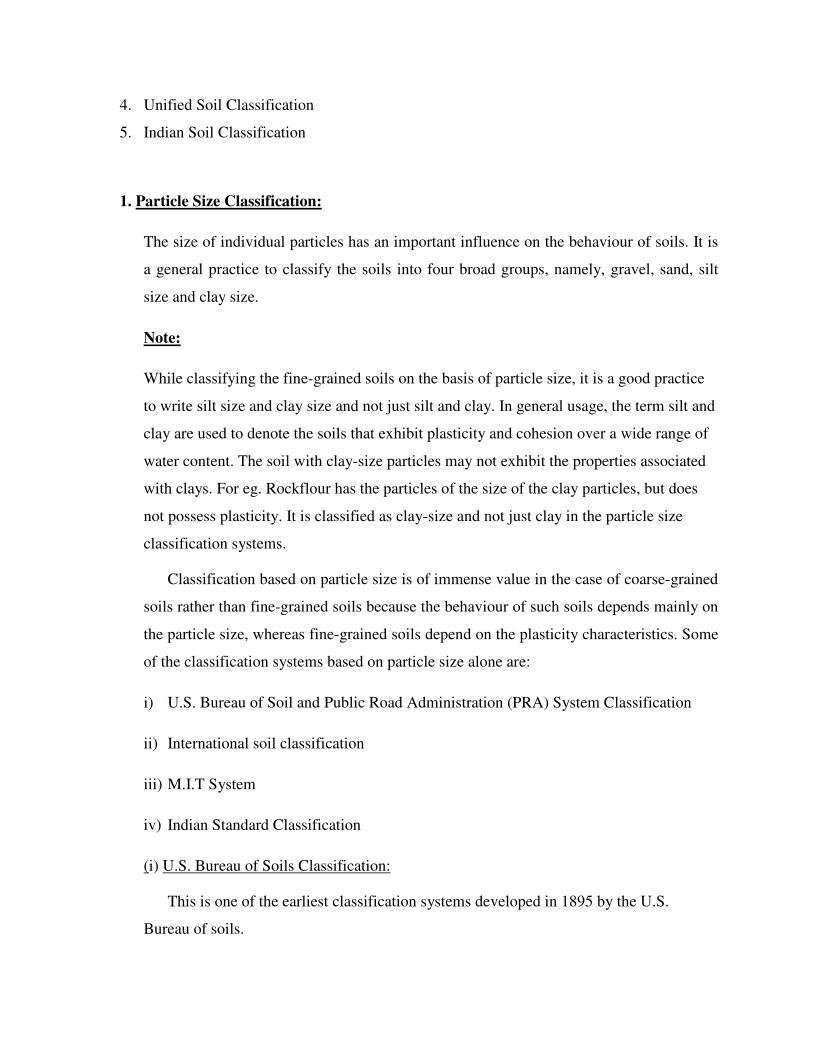
(i) U.S. Bureau of Soils Classification:

This is one of the earliest classification systems developed in 1895 by the U.S.

Bureau of soils.

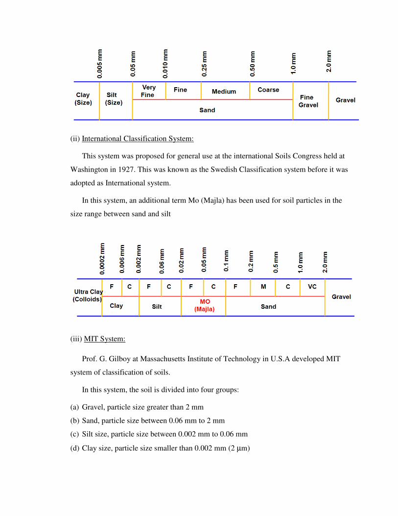
(ii) International Classification System:

This system was proposed for general use at the international Soils Congress held at

Washington in 1927. This was known as the Swedish Classification system before it was

adopted as International system.

In this system, an additional term Mo (Majla) has been used for soil particles in the

size range between sand and silt

(iii) MIT System:

Prof. G. Gilboy at Massachusetts Institute of Technology in U.S.A developed MIT

system of classification of soils.

In this system, the soil is divided into four groups:

(a) Gravel, particle size greater than 2 mm

(b) Sand, particle size between 0.06 mm to 2 mm

(c) Silt size, particle size between 0.002 mm to 0.06 mm

(d) Clay size, particle size smaller than 0.002 mm (2 µm)

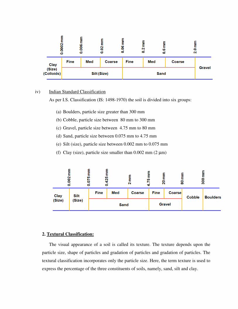
iv) Indian Standard Classification

As per I.S. Classification (IS: 1498-1970) the soil is divided into six groups:

(a) Boulders, particle size greater than 300 mm

(b) Cobble, particle size between 80 mm to 300 mm

(c) Gravel, particle size between 4.75 mm to 80 mm

(d) Sand, particle size between 0.075 mm to 4.75 mm

(e) Silt (size), particle size between 0.002 mm to 0.075 mm

(f) Clay (size), particle size smaller than 0.002 mm (2 µm)

2. Textural Classification:

The visual appearance of a soil is called its texture. The texture depends upon the

particle size, shape of particles and gradation of particles and gradation of particles. The

textural classification incorporates only the particle size. Here, the term texture is used to

express the percentage of the three constituents of soils, namely, sand, silt and clay.

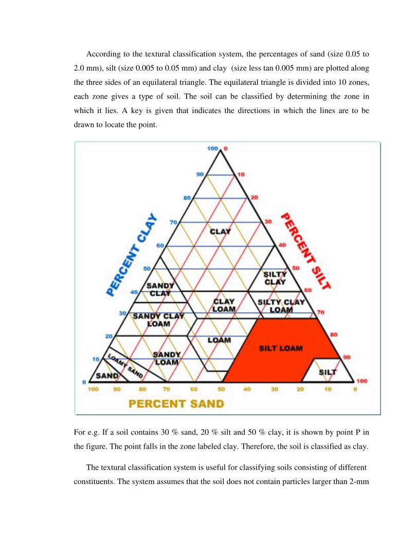
According to the textural classification system, the percentages of sand (size 0.05 to

2.0 mm), silt (size 0.005 to 0.05 mm) and clay (size less tan 0.005 mm) are plotted along

the three sides of an equilateral triangle. The equilateral triangle is divided into 10 zones,

each zone gives a type of soil. The soil can be classified by determining the zone in

which it lies. A key is given that indicates the directions in which the lines are to be

drawn to locate the point.

For e.g. If a soil contains 30 % sand, 20 % silt and 50 % clay, it is shown by point P in

the figure. The point falls in the zone labeled clay. Therefore, the soil is classified as clay.

The textural classification system is useful for classifying soils consisting of different

constituents. The system assumes that the soil does not contain particles larger than 2-mm

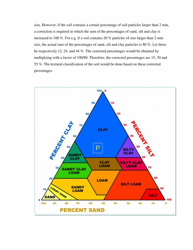
size. However, if the soil contains a certain percentage of soil particles larger than 2 mm,

a correction is required in which the sum of the percentages of sand, silt and clay is

increased to 100 %. For e.g. if a soil contains 20 % particles of size larger than 2-mm

size, the actual sum of the percentages of sand, silt and clay particles is 80 %. Let these

be respectively 12, 24, and 44 %. The corrected percentages would be obtained by

multiplying with a factor of 100/80. Therefore, the corrected percentages are 15, 30 and

55 %. The textural classification of the soil would be done based on these corrected

percentages.

Q 1. How are soils classified based on the Indian Standards Classification. List the salient

features of this classification.

Q 2. What is plasticity chart? Explain how it is useful for classification of fine-grained soils

5) Indian Standard Soil Classification System:

Indian Standard Soil Classification system is in many respects similar to the Unified

system. However, there is one basic difference in the classification of fine-grained soils.

The fine-grained soils in this system are sub-dived into three categories of low, medium

and high compressibility instead of two categories of low and high compressibility in

Unified soil classification system.

Soils are divided into three broad divisions:

1) Coarse-grained soils, when 50 % or more of the total material by weight retained on

75 µm IS sieve.

2) Fine-grained soils, when more than 50 % of the total material passes 75 µm IS sieve.

3) If the soil is highly organic and contains a large percentage of organic matter and

particles of decomposed vegetation, it is kept in a separate category marked as peat

(Pt)

In all, there are 18 groups of soils

Coarse-grained soils – 8 groups

Fine-grained soils – 9 groups

Peat - 1 group

Coarse-Grained Soils:

The classification of coarse-grained soils is done on the basis of their grain and gradation

characteristics as illustrated in Table, when the fines (75 µm) present in them are less

than 5 % by weight. Coarse-grained soils are sub-dived into gravel and sand. The soil is

termed gravel (G) when more than 50 % of coarse fraction (>75 µm) is retained on 4.75

mm IS sieve, and termed sand (S) if more than 50 % of coarse fraction is smaller than

4.75 mm IS sieve. These are further sub-divided as given in Table into 8 groups.

Coarse-grained soils which contain more than 12 % fines (< 75 µm) are classified as

GM or SM if fines are silty in character (meaning, the limits plot below the A-line on the

plasticity chart). On the other hand they are classified as GC or SC if the fines are clayey

in character (meaning the limits plot above the A-line on the plasticity chart).

Fine-grained Soils:

The fine-grained soils are classified on the basis of their plasticity characteristics using

the I.S Plasticity chart shown in Fig.

The fine-grained soils are further divided into three sub-divisions depending upon the

values of the liquid limit:

a) Silts and clays of low compressibility – These soils have a liquid limit less than 35 %

(represented by a symbol L)

b) Silts and clays of medium compressibility – These soils have a liquid limit > 35 %

but < 50 % ( represented by a symbol I)

c) Silts and clays of high compressibility – These soils have a liquid limit > 35 %

(represented by a symbol H)

Fine-grained soils are further sub-divided, as given in table in 9 groups.

Boundary Classifications:

Sometimes, it is not possible to classify to classify a soil into any one of 18 groups

discussed above. A soil may possess characteristics of two groups, either in particle

distribution or in plasticity. For such cases, boundary classifications occur and dual

symbols are used.

a) Boundary classification for coarse-grained soils:

Coarse-grained soils having 5 % to 12 % fines are borderline cases and given a dual

symbol. While giving dual symbols, first assume a coarse soil and then a finer soil i.e.,

the first part of the symbol is indicative of the gradation of coarse fraction, while the

second part indicates the nature of fines.

For example, a soil with the dual symbol SW-SC is a well-graded sand with ‘clayey’

fines that plot above A-line.

(i) Boundary classifications within gravel or sand groups can occur. The following

classification are common

GW-GP, GM-GC, GW-GM, GW-GC, GP-GM,

SW-SP, SM-SC, SW-SM, SW-SC, SP-SM.

(ii) Boundary classifications can occur between the gravel and sand groups such as

GW-SW, GP-SP, GM-SM, and GC-SC

Note: The rule for correct classification is to favour the non-plastic classification.

For eg. A gravel with 10 % fines, Cu = 20 and Cc = 2 and IP= 6 will be classified as GW –

GM, and not GW – GC.

b) Boundary classification for fine-grained soils:

Fine-grained soils also can have dual symbols.

(i) If the limits plot in the hatched zone on the plasticity chart, i.e., IP between 4 and

7, the soil has a group symbol CL – ML.

(ii) If the position of the soil on the plasticity chart falls close to the A-line, dual

symbol is used, such as CI – MI , CH – MH

(iii) If the liquid limit is very close to 35 % or 50 %, dual symbols are used, such as

ML – MI, MI – MH, CL – CI, CI – CH, OL – OI, OI – OH.

c) Boundary classification between coarse-grained and fine-grained soils:

Dual symbols can also be used when the soils have about equal percentage of coarse –

grained and fine – grained fractions. The possible dual symbols in this case are GM –

ML, GM – MI, GM – MH, GC – CL, GC – CI, GC – CH,

SM – ML, SM – MI, SM – MH, SC – CL, SC – CI, SC – CH.

Step-by-step procedure:

A step-by-step procedure for classifying the soils as per IS: 1498 –1970 is illustrated

below:

1. Determine whether the given soil is of organic origin or coarse-grained or fine-

grained. An organic soil is identified by its colour (brownish black or dark) and

characteristic odour. If 50 % or more of the soil by weight is retained on the 75 µm

sieve, it is coarse-grained, if not, it is fine-grained.

2. If the soil is coarse-grained:

(a) Obtain the GSD curve from a sieve-analysis. If 50 % or more of the coarse

fraction (>75 µm) is retained on the 4.75 mm sieve, classify the soil as gravel (G);

if not, classify it as sand (S)

(b) If the soil fraction passing through the 75 µm sieve is less than 5 %, determine the

gradation of the soil by calculating Cu and Cc from the GSD curve. If well graded

(according to the criteria laid down), classify the soil as GW or SW; if poorly

graded, classify as GP or SP.

(c) If more than 12 % passes through the 75 µm sieve, perform the liquid limit and

plastic limit tests on the soil fraction passing though the 0.425-mm sieve. Use the

I.S. plasticity chart to determine the classification (GM, SM, GC, SC, GM – GC

or SM – SC)

(d) If between 5 % and 12 % passes through the 75 µm sieve, the soil is assigned a

dual symbol appropriate to its gradation and plasticity characteristics. (GW – GW,

GW – GC, GP – GC, GP – GW, GM, SW - SM, SW - SC, SP – SC, SP - SM)

3. If the soil is fine-grained (inorganic):

(a) Determine wL and wP on the minus 0.425 mm sieve fraction and determine the

plasticity index.

(b) If the limits plot below the A – line, classify as silt (M). Further, if wL is less than

35, classify as ML; if wL is between 35 – 50 %, classify as MI; if wL is greater

than 50, classify as MH.

(c) If the limits plot above the A – line, classify as clay ©. Assign the group symbol

CL or CI or CH, depending on the value of liquid limit, as in (b).

(d) If the limits plot in the hatched zone, classify as CL – ML. If the limits plot close

to the A – line or close to wL= 35 % or wL= 50 % lines, assign dual symbols as

outlined earlier.

4. If the soil is of organic origin, the plasticity chart is used after determining wL and wP

and the soil classified as OL, OI or OH.

5. If the soil has about 50 % each of fines and coarse – grained fractions,

(a) Determine whether the coarse – grained fraction is gravel (G) or sand (S)

(b) Determine wL and wP on the minus 0.425 mm fraction

(c) Depending on whether the limits plot above the A – line or below the A – line,

classify as C or M

(d) Based on wL, classify as L, I or H

(e) Assign the dual symbol from the information obtained in steps (a), (b), (c), and

(d) as for example, GM – ML, GM – MI, etc.,

Field identification of soils

Basically, coarse-grained and fine-grained soils are distinguished based on whether

the individual soil grains can be seen with naked eye or not. Thus, grain-size itself may be

adequate to distinguish between gravel and sand; but silt and clay cannot be distinguished by

this technique.

Field identification of soils becomes easier if one understands how to distinguish

gravel from sand, sand from silt, and silt from clay.

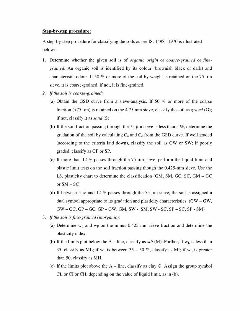
Gravel from sand:

Individual soil particles larger than 4.75 mm and smaller than 80 mm are called

‘Gravel”; soil particles ranging in size from 4.75 mm down to 0.075 mm are called ‘Sand’.

These limits although arbitrary in nature have been accepted widely. The shape of these

particles is also important and may be described as angular, sub-angular, rounded, etc. Filed

identification of sand and gravel should also include identification of mineralogical

composition, if possible.

GRAVEL SAND

Sand from Silt:

Fine sand cannot be easily distinguished from silt by simple visual examination. Silt

may look a little darker in colour. However, it is possible to differentiate between the two by

the ‘Dispersion test’. This test consists of pouring a spoonful of sample in a jar of water. If

the material is sand, it will settle down in a minute or two, but, it will settle down in a minute

or two, but, if it is silt, it may take 15 minutes to one hour to settle. In both these cases

nothing may be left in the suspension ultimately.

Silt from Clay:

(i) Dilatancy test:

It consists of placing a pat of moist soil in the palm of the hand, and then shaking the

hand. If a shiny, moist surface appears on the soil after shaking it in the open hand

and then becomes dull and dry when the pat is squeezed by closing the hand, a non-

plastic soil (e.g. silt) is indicated.

Note: squeezing the pat causes shearing deformations in the soil, which in turn cause

a non-plastic soil to expand from low volume obtained by shaking. The water flows

into the soil to make up for the increased volume of pores and, thereby, leaves the

surface with a dry appearance.

If it is clay, the water cannot move easily and hence, it continues to look dark. If it is

a mixture of silt and clay, the relative speed with which the shine appears may give a

rough indication of the amount of silt present. This test is also known as ‘shaking test’

or ‘water mobility test’.

(ii) Strength test:

A small lump of the soil is dried slowly. Then the dry lump is tested for its dry

strength by trying to powder the lump between the fingers. If it can be broken easily

or powdered with the fingers, the material is silt. If it is clay, it will require effort to

break. Also, if it is silt one can dust off loose material from the surface of the lump.

When moist soil is pressed between fingers, clay gives a soapy touch; it also sticks to

the fingers, dries slowly, and cannot be dusted off easily.

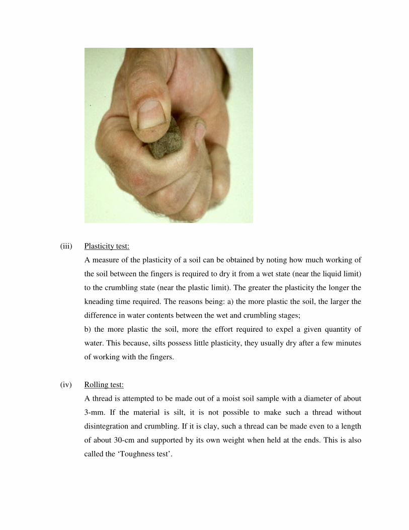
(iii) Plasticity test:

A measure of the plasticity of a soil can be obtained by noting how much working of

the soil between the fingers is required to dry it from a wet state (near the liquid limit)

to the crumbling state (near the plastic limit). The greater the plasticity the longer the

kneading time required. The reasons being: a) the more plastic the soil, the larger the

difference in water contents between the wet and crumbling stages;

b) the more plastic the soil, more the effort required to expel a given quantity of

water. This because, silts possess little plasticity, they usually dry after a few minutes

of working with the fingers.

(iv) Rolling test:

A thread is attempted to be made out of a moist soil sample with a diameter of about

3-mm. If the material is silt, it is not possible to make such a thread without

disintegration and crumbling. If it is clay, such a thread can be made even to a length

of about 30-cm and supported by its own weight when held at the ends. This is also

called the ‘Toughness test’.

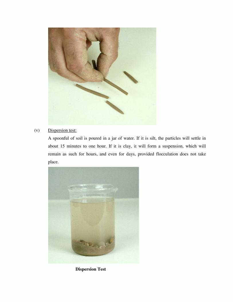
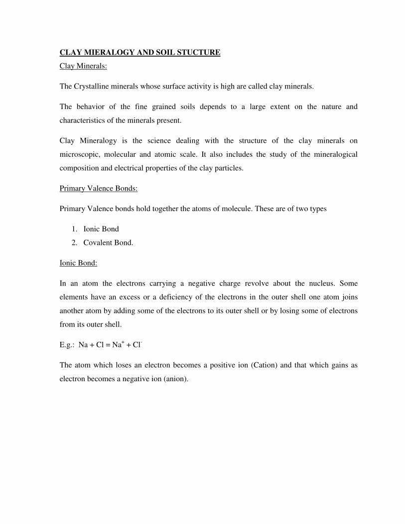
(v) Dispersion test:

A spoonful of soil is poured in a jar of water. If it is silt, the particles will settle in

about 15 minutes to one hour. If it is clay, it will form a suspension, which will

remain as such for hours, and even for days, provided flocculation does not take

place.

Dispersion Test

A few other miscellaneous identification tests are as follows:

Organic content and colour:

Fresh, wet organic soils usually have a distinctive odour of decomposed organic

matter, which can be easily detected on heating. Another distinctive feature of such soils is

the dark colour.

Acid test:

This test, using dilute HCl, is primarily for checking the presence of calcium

carbonate. For soils with a high value of dry strength, a strong reaction may indicate the

presence of calcium carbonate as cementing material rather than colloidal clay.

Shine test:

When a lump of dry or slightly moist soil is cut with a knife, a shiny surface is

imparted to the soil if it is highly plastic clay, while a dull surface may indicate silt or clay of

low plasticity.

CLAY MIERALOGY AND SOIL STUCTURE

Clay Minerals:

The Crystalline minerals whose surface activity is high are called clay minerals.

The behavior of the fine grained soils depends to a large extent on the nature and

characteristics of the minerals present.

Clay Mineralogy is the science dealing with the structure of the clay minerals on

microscopic, molecular and atomic scale. It also includes the study of the mineralogical

composition and electrical properties of the clay particles.

Primary Valence Bonds:

Primary Valence bonds hold together the atoms of molecule. These are of two types

1. Ionic Bond

2. Covalent Bond.

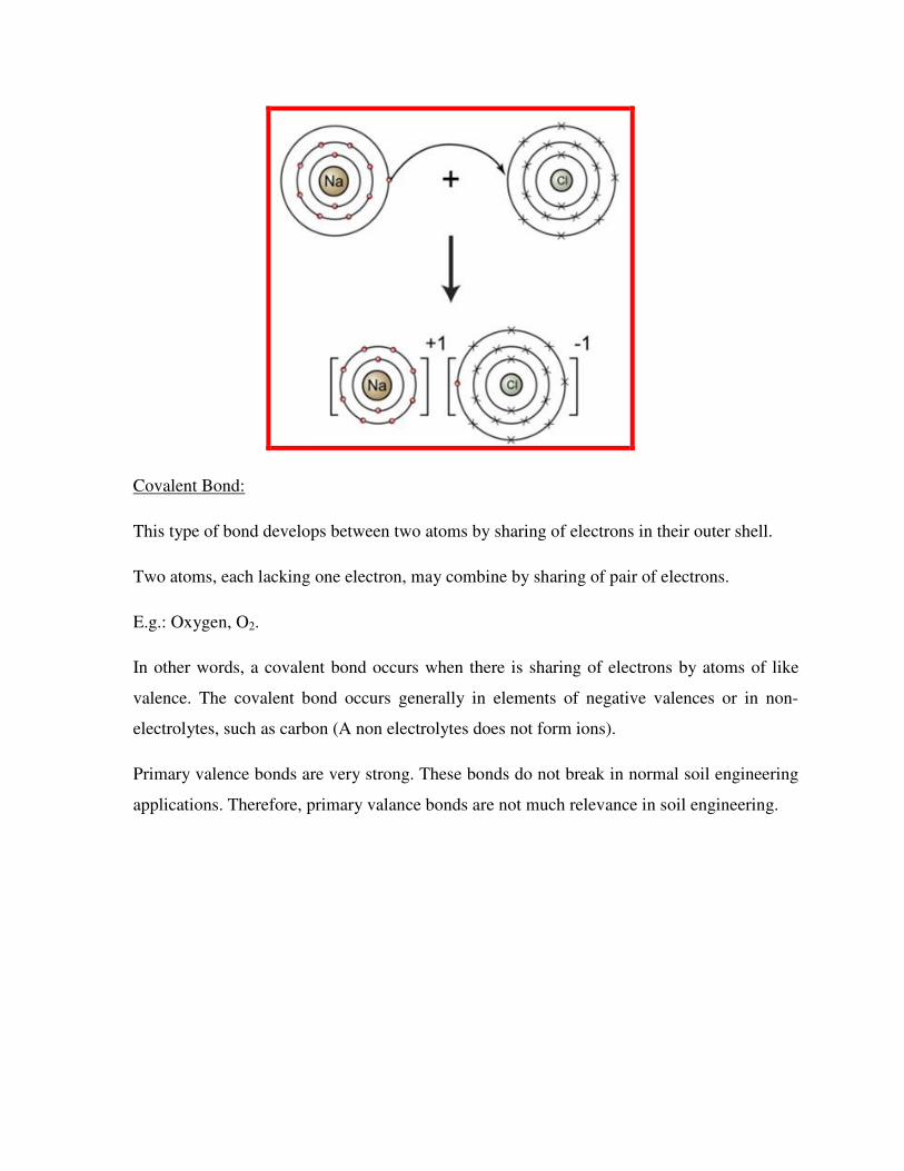
Ionic Bond:

In an atom the electrons carrying a negative charge revolve about the nucleus. Some

elements have an excess or a deficiency of the electrons in the outer shell one atom joins

another atom by adding some of the electrons to its outer shell or by losing some of electrons

from its outer shell.

E.g.: Na + Cl = Na+ + Cl-

The atom which loses an electron becomes a positive ion (Cation) and that which gains as

electron becomes a negative ion (anion).

Covalent Bond:

This type of bond develops between two atoms by sharing of electrons in their outer shell.

Two atoms, each lacking one electron, may combine by sharing of pair of electrons.

E.g.: Oxygen, O2.

In other words, a covalent bond occurs when there is sharing of electrons by atoms of like

valence. The covalent bond occurs generally in elements of negative valences or in non-

electrolytes, such as carbon (A non electrolytes does not form ions).

Primary valence bonds are very strong. These bonds do not break in normal soil engineering

applications. Therefore, primary valance bonds are not much relevance in soil engineering.

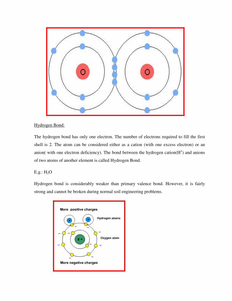
Hydrogen Bond:

The hydrogen bond has only one electron. The number of electrons required to fill the first

shell is 2. The atom can be considered either as a cation (with one excess electron) or an

anion( with one electron deficiency). The bond between the hydrogen cation(H+) and anions

of two atoms of another element is called Hydrogen Bond.

E.g.: H2O

Hydrogen bond is considerably weaker than primary valence bond. However, it is fairly

strong and cannot be broken during normal soil engineering problems.

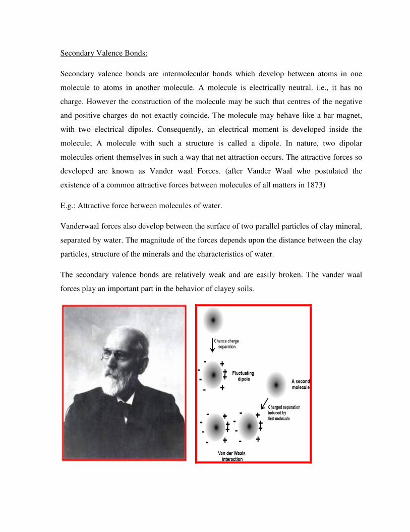
Secondary Valence Bonds:

Secondary valence bonds are intermolecular bonds which develop between atoms in one

molecule to atoms in another molecule. A molecule is electrically neutral. i.e., it has no

charge. However the construction of the molecule may be such that centres of the negative

and positive charges do not exactly coincide. The molecule may behave like a bar magnet,

with two electrical dipoles. Consequently, an electrical moment is developed inside the

molecule; A molecule with such a structure is called a dipole. In nature, two dipolar

molecules orient themselves in such a way that net attraction occurs. The attractive forces so

developed are known as Vander waal Forces. (after Vander Waal who postulated the

existence of a common attractive forces between molecules of all matters in 1873)

E.g.: Attractive force between molecules of water.

Vanderwaal forces also develop between the surface of two parallel particles of clay mineral,

separated by water. The magnitude of the forces depends upon the distance between the clay

particles, structure of the minerals and the characteristics of water.

The secondary valence bonds are relatively weak and are easily broken. The vander waal

forces play an important part in the behavior of clayey soils.

Van der Waal

Basic structural units of clay minerals or primary building blocks of clay minerals.

CLay minerals are composed of two basic structural units.

1. Tetrahedral Unit

2. Octahedral Unit.

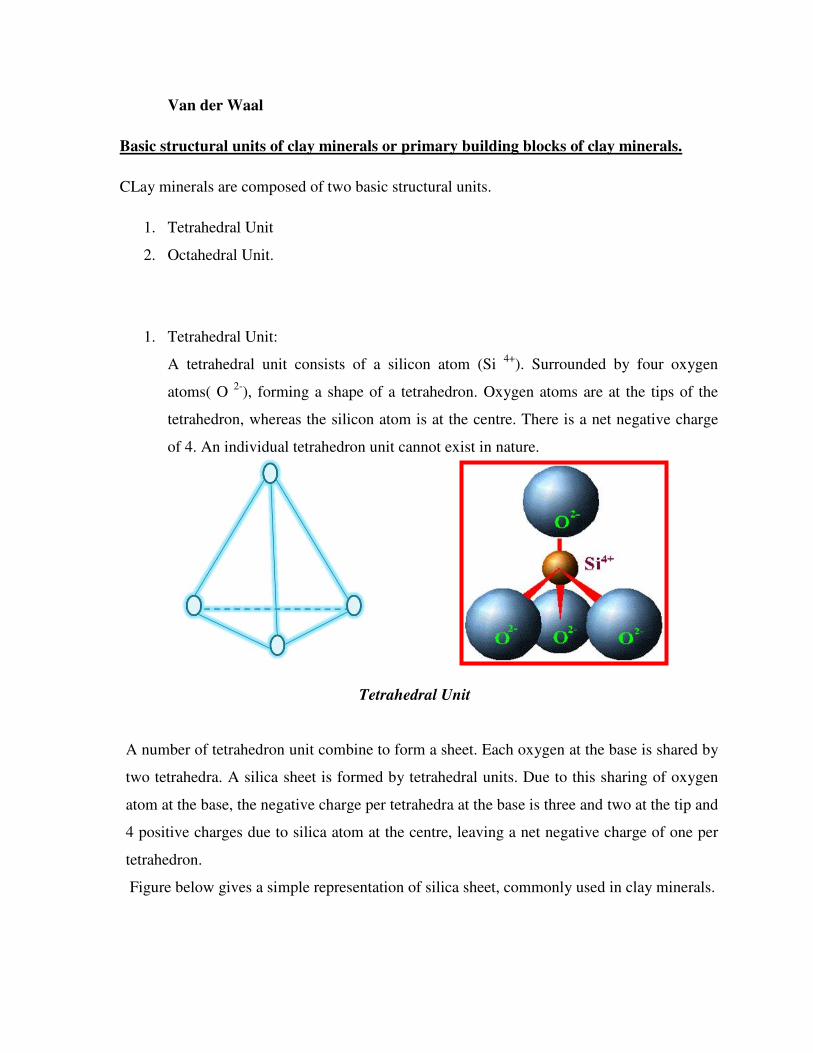
1. Tetrahedral Unit:

A tetrahedral unit consists of a silicon atom (Si 4+). Surrounded by four oxygen

atoms( O 2-), forming a shape of a tetrahedron. Oxygen atoms are at the tips of the

tetrahedron, whereas the silicon atom is at the centre. There is a net negative charge

of 4. An individual tetrahedron unit cannot exist in nature.

Tetrahedral Unit

A number of tetrahedron unit combine to form a sheet. Each oxygen at the base is shared by

two tetrahedra. A silica sheet is formed by tetrahedral units. Due to this sharing of oxygen

atom at the base, the negative charge per tetrahedra at the base is three and two at the tip and

4 positive charges due to silica atom at the centre, leaving a net negative charge of one per

tetrahedron.

Figure below gives a simple representation of silica sheet, commonly used in clay minerals.

2. Octahedral Unit:

It consists of six hydroxyles (OH-) forming a configuration of an octahedron and

having one aluminium atom at the centre. As the aluminum (Al +3) has three positive

charges, an octahedral unit has 3 negative charges. Because of net negative charges,

an octahedral unit cannot exist in isolation.

Octahedral Unit

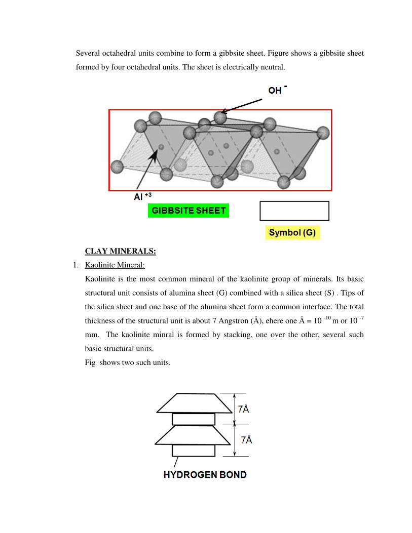
Several octahedral units combine to form a gibbsite sheet. Figure shows a gibbsite sheet

formed by four octahedral units. The sheet is electrically neutral.

CLAY MINERALS:

1. Kaolinite Mineral:

Kaolinite is the most common mineral of the kaolinite group of minerals. Its basic

structural unit consists of alumina sheet (G) combined with a silica sheet (S) . Tips of

the silica sheet and one base of the alumina sheet form a common interface. The total

thickness of the structural unit is about 7 Angstron (Å), ehere one Å = 10 -10 m or 10 -7

mm. The kaolinite minral is formed by stacking, one over the other, several such

basic structural units.

Fig shows two such units.

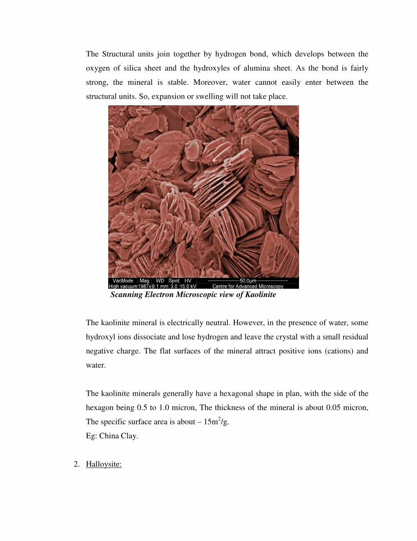
The Structural units join together by hydrogen bond, which develops between the

oxygen of silica sheet and the hydroxyles of alumina sheet. As the bond is fairly

strong, the mineral is stable. Moreover, water cannot easily enter between the

structural units. So, expansion or swelling will not take place.

Scanning Electron Microscopic view of Kaolinite

The kaolinite mineral is electrically neutral. However, in the presence of water, some

hydroxyl ions dissociate and lose hydrogen and leave the crystal with a small residual

negative charge. The flat surfaces of the mineral attract positive ions (cations) and

water.

The kaolinite minerals generally have a hexagonal shape in plan, with the side of the

hexagon being 0.5 to 1.0 micron, The thickness of the mineral is about 0.05 micron,

The specific surface area is about – 15m2/g.

Eg: China Clay.

2. Halloysite:

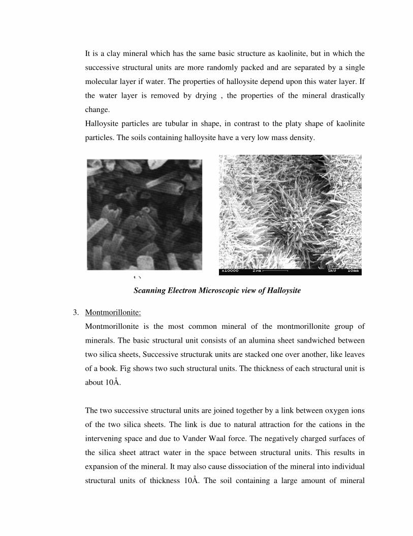
It is a clay mineral which has the same basic structure as kaolinite, but in which the

successive structural units are more randomly packed and are separated by a single

molecular layer if water. The properties of halloysite depend upon this water layer. If

the water layer is removed by drying , the properties of the mineral drastically

change.

Halloysite particles are tubular in shape, in contrast to the platy shape of kaolinite

particles. The soils containing halloysite have a very low mass density.

Scanning Electron Microscopic view of Halloysite

3. Montmorillonite:

Montmorillonite is the most common mineral of the montmorillonite group of

minerals. The basic structural unit consists of an alumina sheet sandwiched between

two silica sheets, Successive structurak units are stacked one over another, like leaves

of a book. Fig shows two such structural units. The thickness of each structural unit is

about 10Å.

The two successive structural units are joined together by a link between oxygen ions

of the two silica sheets. The link is due to natural attraction for the cations in the

intervening space and due to Vander Waal force. The negatively charged surfaces of

the silica sheet attract water in the space between structural units. This results in

expansion of the mineral. It may also cause dissociation of the mineral into individual

structural units of thickness 10Å. The soil containing a large amount of mineral

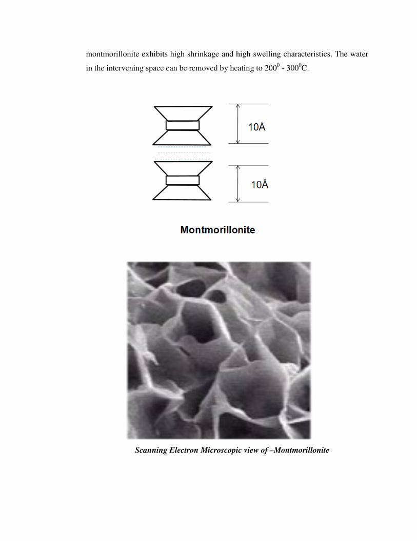
montmorillonite exhibits high shrinkage and high swelling characteristics. The water

in the intervening space can be removed by heating to 2000 - 3000C.

Scanning Electron Microscopic view of –Montmorillonite

Montmorillonite minerals have lateral dimensions of 0.1µ to 0.5µ and the thickness of

0.001µ to 0.005µ. The specific surface is about 800m2/g.

The gibbsite sheet in a montmorillonite mineral may contain iron or magnesium

instead of aluminium. Some of the silicon atoms in the silica sheet may also have

isomorphous substitution. This results in giving the mineral a residual negative

charge. It attracts water to form an adsorbed layer, which gives plasticity

characteristics to the soil.

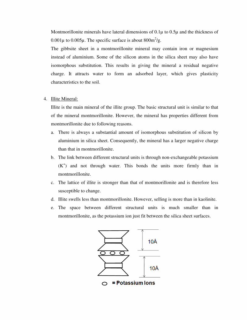
4. Illite Mineral:

Illite is the main mineral of the illite group. The basic structural unit is similar to that

of the mineral montmorillonite. However, the mineral has properties different from

montmorillonite due to following reasons.

a. There is always a substantial amount of isomorphous substitution of silicon by

aluminium in silica sheet. Consequently, the mineral has a larger negative charge

than that in montmorillonite.

b. The link between different structural units is through non-exchangeable potassium

(K+) and not through water. This bonds the units more firmly than in

montmorillonite.

c. The lattice of illite is stronger than that of montmorillonite and is therefore less

susceptible to change.

d. Illite swells less than montmorillonite. However, selling is more than in kaolinite.

e. The space between different structural units is much smaller than in

montmorillonite, as the potassium ion just fit between the silica sheet surfaces.

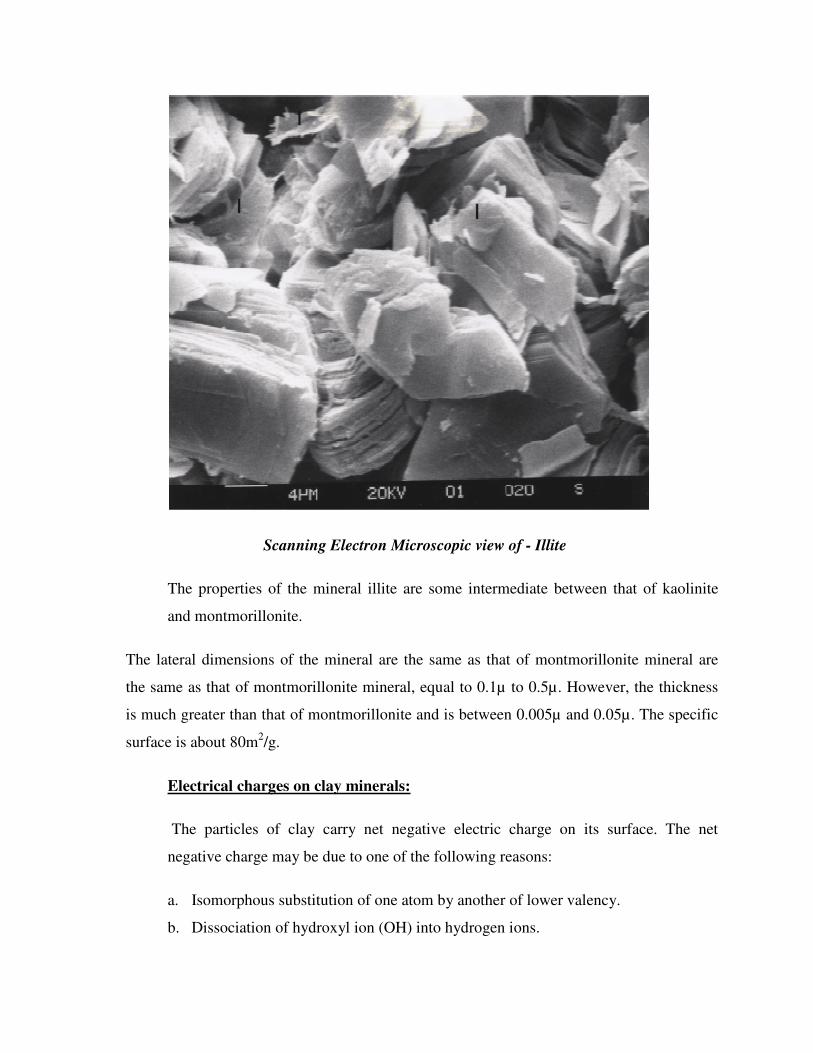
Scanning Electron Microscopic view of - Illite

The properties of the mineral illite are some intermediate between that of kaolinite

and montmorillonite.

The lateral dimensions of the mineral are the same as that of montmorillonite mineral are

the same as that of montmorillonite mineral, equal to 0.1µ to 0.5µ. However, the thickness

is much greater than that of montmorillonite and is between 0.005µ and 0.05µ. The specific

surface is about 80m2/g.

Electrical charges on clay minerals:

The particles of clay carry net negative electric charge on its surface. The net

negative charge may be due to one of the following reasons:

a. Isomorphous substitution of one atom by another of lower valency.

b. Dissociation of hydroxyl ion (OH) into hydrogen ions.

c. Adsorption of anions (negative ions) on the edge of clay particles.

d. Absence of cations (positive ions) in the lattice of the crystal.

e. Presence of organic matter.

The magnitude of the electrical charge depends on the surface area of the particle.

It is very high in small particles, such as colloids, which have very large surface

area. A soil attracts the cations in the environment to neutralize the negative

charge. The phenomenon is known as adsorption.

Base Exchange capacity:

The cations attracted to the negatively charged surface of the soil particles are not

strongly attached. These cations can be replaced by other ions and are, therefore known as

exchangeable ions. The phenomenon of replacement of cations is called cation exchange or

base exchange.

The net negative charge on the mineral which can be satisfied by exchangeable

cations is termed cation exchange capacity (CEC) or base exchange capacity (BEC).

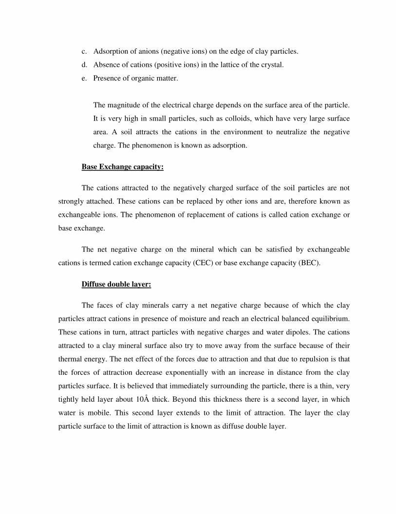
Diffuse double layer:

The faces of clay minerals carry a net negative charge because of which the clay

particles attract cations in presence of moisture and reach an electrical balanced equilibrium.

These cations in turn, attract particles with negative charges and water dipoles. The cations

attracted to a clay mineral surface also try to move away from the surface because of their

thermal energy. The net effect of the forces due to attraction and that due to repulsion is that

the forces of attraction decrease exponentially with an increase in distance from the clay

particles surface. It is believed that immediately surrounding the particle, there is a thin, very

tightly held layer about 10Å thick. Beyond this thickness there is a second layer, in which

water is mobile. This second layer extends to the limit of attraction. The layer the clay

particle surface to the limit of attraction is known as diffuse double layer.

Diffuse Double Layer

In other words, base exchange capacity is the capacity of the clay particles to change the

cation adsorbed on the surface.

BEC is expresses in terms of the total number of positive charges adsorbed per 100g of soil.

It is measured in milliequivalent (meq), which is equal to 6 X 1020 electronic charges. (Thus,

one meq per 100g means that 100 g of material can exchange 6 X 1020 electronic charges if

the exchangeable ions are univalent, such as Na+. However, it is the exchangeable ions are

divalent, such as Ca2+, 100g of material will replace 3 X 1020 calcium ions)

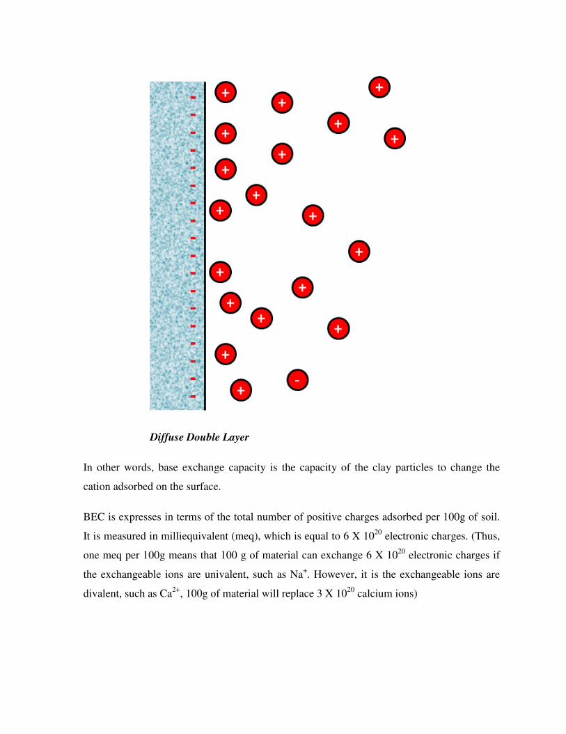
Cation Adsorption

The Base Exchange Capacity of clay depends upon the pH value of the water in the

environment. If the water is acidic (pH < 7), the BEC is reduced. Some cations are more

strongly adsorbed than others. The adsorbed cations commonly found in soils, arranged in a

series in terms of their affinity for attraction are as follows:

Al3+ > Ca2+ > Mg+2 >NH4+>K+ > H+>Na+> Li+

For e.g.,: Al +3 cations are more strongly attracted than Ca2+ cations. Thus Al 3+ ions can

replace Ca2+ ions. Likewise Ca2+ ions can replace Na+ ions.

Adsorbed Water:

The water held by electro-chemical forces existing on the soil surface is known as adsorbed

water. As the adsorbed water is under the influence of electrical forces, its properties are

different from normal water. It is much more viscous, and its surface tension is also greater.

It is heavier than normal water. The boiling point is higher, but the freezing point is lower

than that of the normal water.

The thickness of adsorbed water layer is usually about 10 to 15Å. This water imparts

plasticity characteristics to soils.

Soil Structure:

The geometrical arrangement of soil particles with respect to one another in a soil mass is

known as soil structure.

Engineering properties and the behavior of both coarse grained and fine grained soils depend

upon the soil structure.

The following types of structures are usually found.

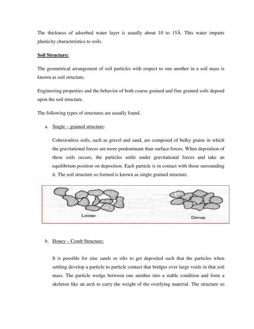
a. Single – grained structure:

Cohesionless soils, such as gravel and sand, are composed of bulky grains in which

the gravitational forces are more predominant than surface forces. When deposition of

these soils occurs, the particles settle under gravitational forces and take an

equilibrium position on deposition. Each particle is in contact with those surrounding

it. The soil structure so formed is known as single grained structure.

b. Honey – Comb Structure:

It is possible for sine sands or silts to get deposited such that the particles when

settling develop a particle to particle contact that bridges over large voids in that soil

mass. The particle wedge between one another into a stable condition and form a

skeleton like an arch to carry the weight of the overlying material. The structure so

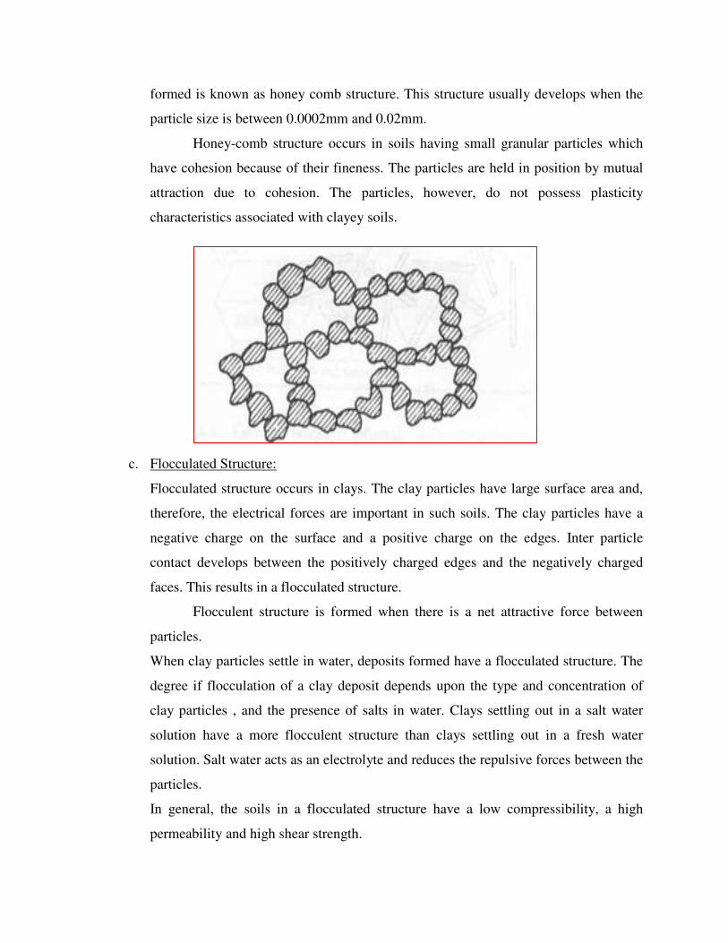
formed is known as honey comb structure. This structure usually develops when the

particle size is between 0.0002mm and 0.02mm.

Honey-comb structure occurs in soils having small granular particles which

have cohesion because of their fineness. The particles are held in position by mutual

attraction due to cohesion. The particles, however, do not possess plasticity

characteristics associated with clayey soils.

c. Flocculated Structure:

Flocculated structure occurs in clays. The clay particles have large surface area and,

therefore, the electrical forces are important in such soils. The clay particles have a

negative charge on the surface and a positive charge on the edges. Inter particle

contact develops between the positively charged edges and the negatively charged

faces. This results in a flocculated structure.

Flocculent structure is formed when there is a net attractive force between

particles.

When clay particles settle in water, deposits formed have a flocculated structure. The

degree if flocculation of a clay deposit depends upon the type and concentration of

clay particles , and the presence of salts in water. Clays settling out in a salt water

solution have a more flocculent structure than clays settling out in a fresh water

solution. Salt water acts as an electrolyte and reduces the repulsive forces between the

particles.

In general, the soils in a flocculated structure have a low compressibility, a high

permeability and high shear strength.

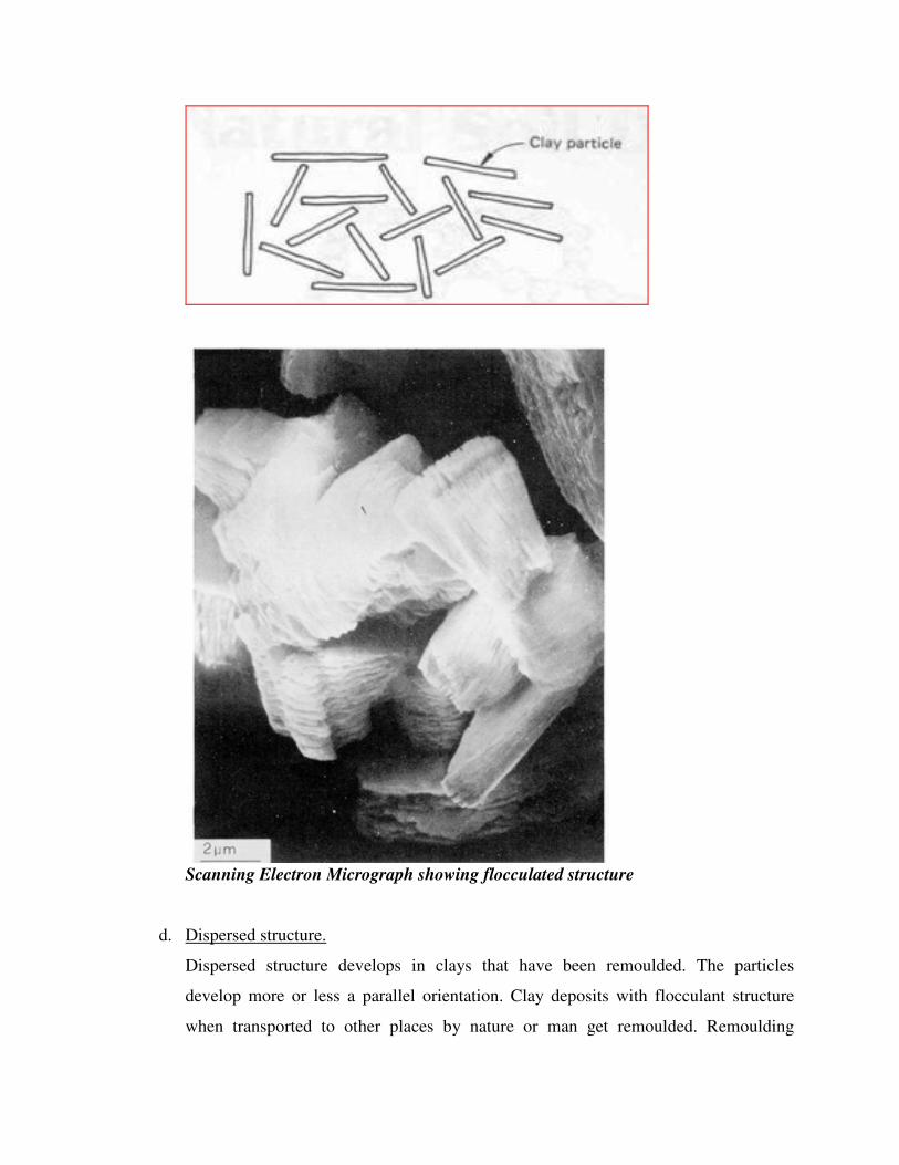
Scanning Electron Micrograph showing flocculated structure

d. Dispersed structure.

Dispersed structure develops in clays that have been remoulded. The particles

develop more or less a parallel orientation. Clay deposits with flocculant structure

when transported to other places by nature or man get remoulded. Remoulding

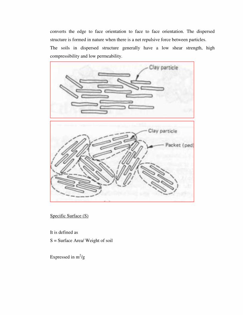
converts the edge to face orientation to face to face orientation. The dispersed

structure is formed in nature when there is a net repulsive force between particles.

The soils in dispersed structure generally have a low shear strength, high

compressibility and low permeability.

Specific Surface (S)

It is defined as

S = Surface Area/ Weight of soil

Expressed in m2/g