Matthew Zengerer

Geostatistically-Constrained 3D Potential Field and Geology Modelling using Drillhole Data

Case Studies from Hydrocarbons and Mineral Exploration

Talk Outline • Introduction – Purpose and Workflow

• Geological and Geostatistical Modelling

• East African Rift Case Study with FTG

• Uranium Case Study with Gravity

• Conclusions

What’s the Job?? • Build a 3D Geological Model from Drilling Data and

additional data (Seismic Horizons, Mapping, Geophysical Interpretation)

• Analyse Formation Properties

• Geostatistically interpolate property data in Model

• Forward Model Geophysical Response

• Compare with Observed Geophysical Data

• Run Inversion

• Report on Outcomes

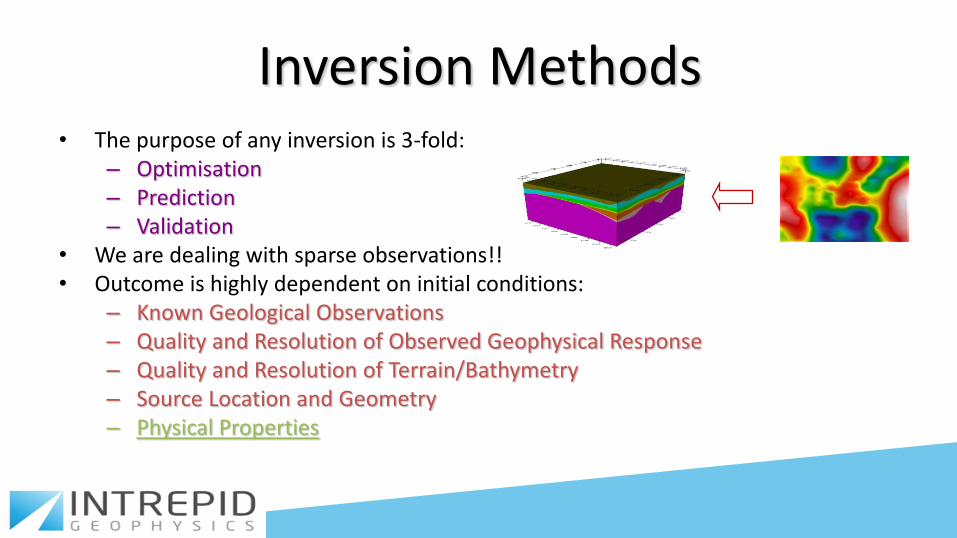
Inversion Methods • The purpose of any inversion is 3-fold:

– Optimisation – Prediction – Validation

• We are dealing with sparse observations!! • Outcome is highly dependent on initial conditions:

– Known Geological Observations – Quality and Resolution of Observed Geophysical Response – Quality and Resolution of Terrain/Bathymetry – Source Location and Geometry – Physical Properties

Geostatistics for Model Construction • Creating a 3D property volume

• Drillhole log data are dense in information but may be sparse in distribution

• Physical and Chemical Properties, can be recorded and related to validate property and lithology models

• Think about Relationships

– If data on one important logging parameter is limited, another parameter may help characterise its behaviour

Model Constraints • 3D Lithology / Property model is

desired

• Interpolation of downhole log properties to generate property voxet

• Solve Problems with properties and geometries

• Build Models using all sources – including proxies and property estimations

• It can drive you a little crazy!!!

Geostatistical Methods • Examine Logs and Property Distributions

• Compute Variograms

• Inverse Distance Weighting

• Kriging 1D and 2D

• Domain Kriging

– Pot (t) Variogram of parameter correlates with 3D formation thickness

– u, v, pot (t) (3D)

• Other techniques eg Gaussian Simulation

Domaining

p1 p2

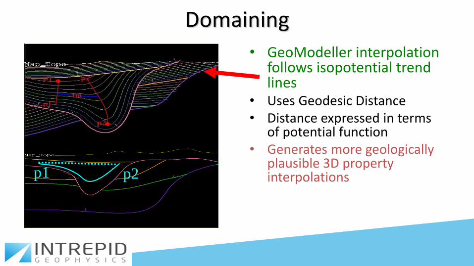
• GeoModeller interpolation follows isopotential trend lines

• Uses Geodesic Distance • Distance expressed in terms

of potential function • Generates more geologically

plausible 3D property interpolations

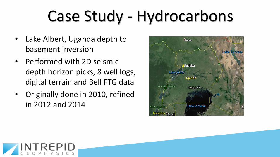
Case Study - Hydrocarbons • Lake Albert, Uganda depth to

basement inversion

• Performed with 2D seismic depth horizon picks, 8 well logs, digital terrain and Bell FTG data

• Originally done in 2010, refined in 2012 and 2014

Case Study – Hydrocarbons Lithology

• Construction of initial 3D Lithology model from 2D seismic depth horizon picks and well formation boundaries

• Model dimensions are 33 x 23 km

Strat

Column

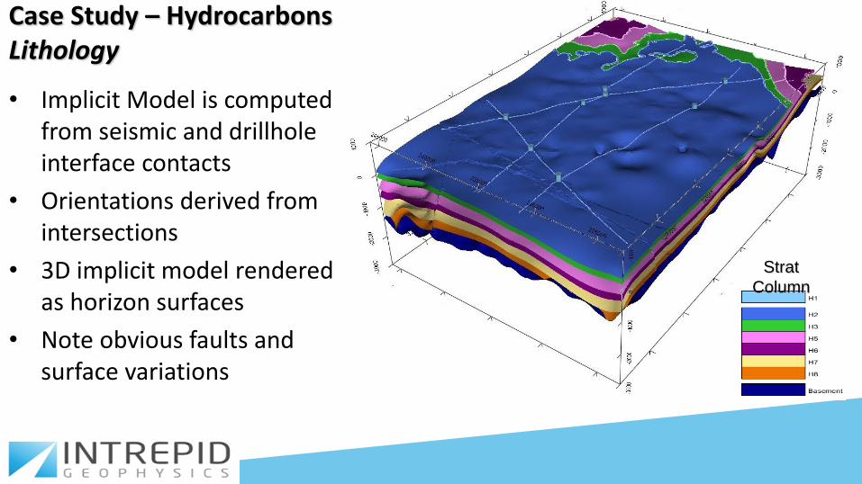
Case Study – Hydrocarbons Lithology

• Implicit Model is computed from seismic and drillhole interface contacts

• Orientations derived from intersections

• 3D implicit model rendered as horizon surfaces

• Note obvious faults and surface variations

Strat

Column

Case Study – Hydrocarbons Lithology

• 3D model showing horizon surfaces and vertical gravity gradient Gzz from FTG survey draped on topography

Strat

Column

Gzz

Eötvös

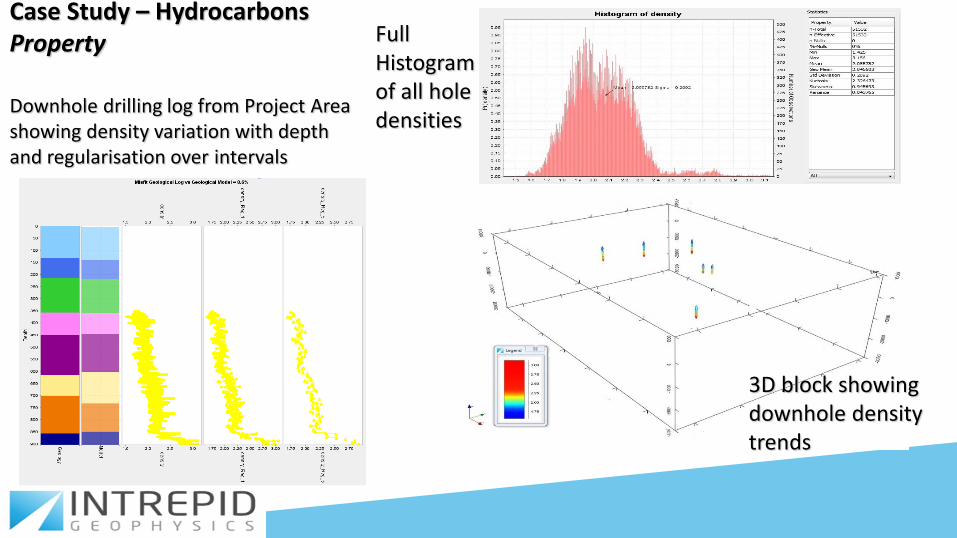
Downhole drilling log from Project Area showing density variation with depth and regularisation over intervals

Full Histogram of all hole densities

3D block showing downhole density trends

Case Study – Hydrocarbons Property

Case Study – Hydrocarbons Property

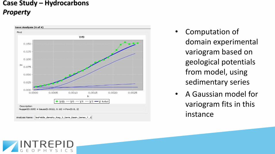
• Computation of domain experimental variogram based on geological potentials from model, using sedimentary series

• A Gaussian model for variogram fits in this instance

Case Study – Hydrocarbons Property

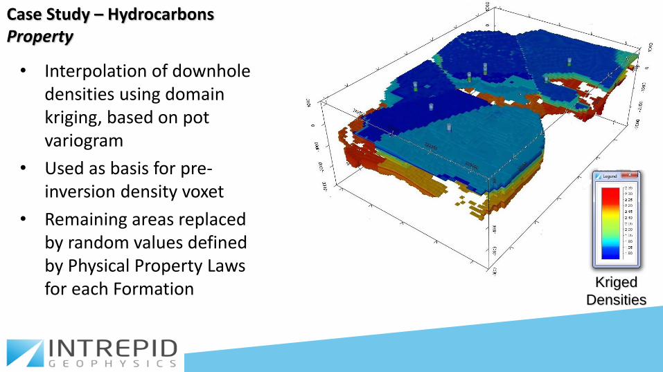
• Interpolation of downhole densities using domain kriging, based on pot variogram

• Used as basis for pre-inversion density voxet

• Remaining areas replaced by random values defined by Physical Property Laws for each Formation Kriged

Densities

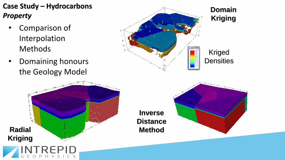
Case Study – Hydrocarbons Property

• Comparison of Interpolation Methods

• Domaining honours the Geology Model

Kriged

Densities

Domain

Kriging

Inverse

Distance

Method Radial

Kriging

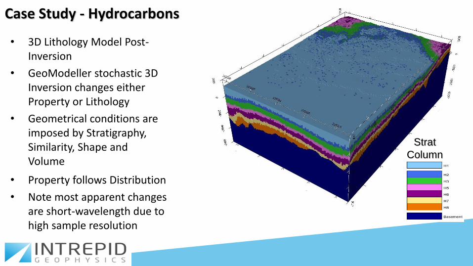
Case Study - Hydrocarbons

• 3D Lithology Model Post-Inversion

• GeoModeller stochastic 3D Inversion changes either Property or Lithology

• Geometrical conditions are imposed by Stratigraphy, Similarity, Shape and Volume

Strat

Column

• Property follows Distribution

• Note most apparent changes are short-wavelength due to high sample resolution

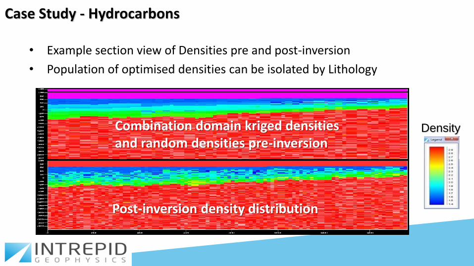
Case Study - Hydrocarbons

• Example section view of Densities pre and post-inversion

• Population of optimised densities can be isolated by Lithology

Density Combination domain kriged densities and random densities pre-inversion

Post-inversion density distribution

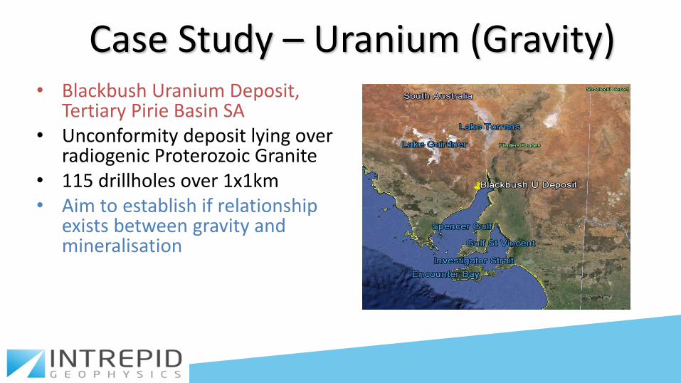
Case Study – Uranium (Gravity) • Blackbush Uranium Deposit,

Tertiary Pirie Basin SA • Unconformity deposit lying over

radiogenic Proterozoic Granite • 115 drillholes over 1x1km • Aim to establish if relationship

exists between gravity and mineralisation

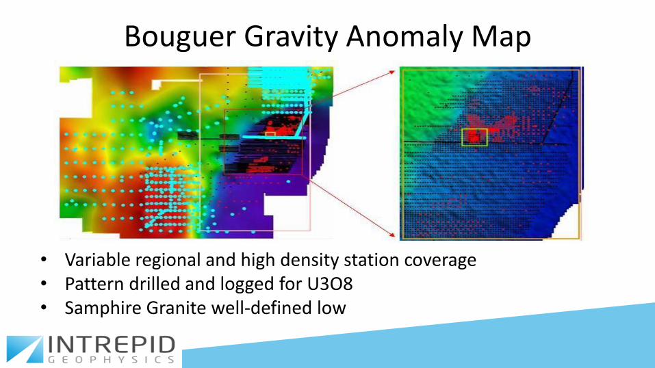
Bouguer Gravity Anomaly Map

• Variable regional and high density station coverage • Pattern drilled and logged for U3O8 • Samphire Granite well-defined low

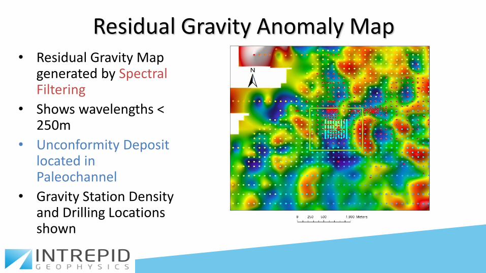
Residual Gravity Anomaly Map • Residual Gravity Map

generated by Spectral Filtering

• Shows wavelengths < 250m

• Unconformity Deposit located in Paleochannel

• Gravity Station Density and Drilling Locations shown

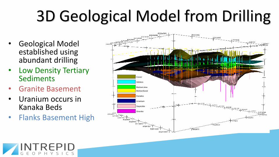
3D Geological Model from Drilling

• Geological Model established using abundant drilling

• Low Density Tertiary Sediments

• Granite Basement • Uranium occurs in

Kanaka Beds • Flanks Basement High

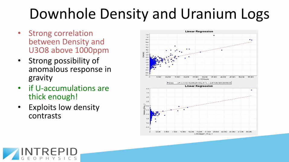
Downhole Density and Uranium Logs • Strong correlation

between Density and U3O8 above 1000ppm

• Strong possibility of anomalous response in gravity

• if U-accumulations are thick enough!

• Exploits low density contrasts

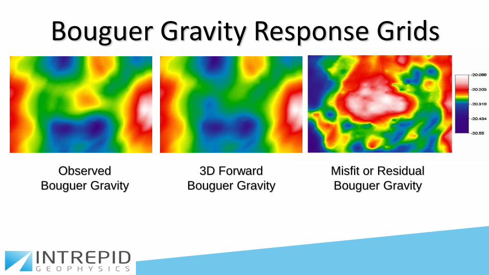
Bouguer Gravity Response Grids

Observed

Bouguer Gravity

3D Forward

Bouguer Gravity

Misfit or Residual

Bouguer Gravity

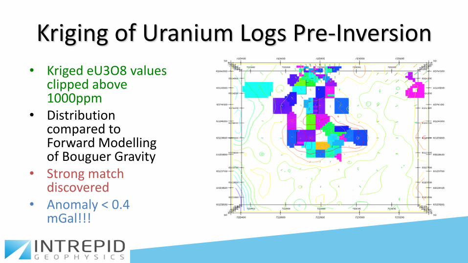
Kriging of Uranium Logs Pre-Inversion

• Kriged eU3O8 values clipped above 1000ppm

• Distribution compared to Forward Modelling of Bouguer Gravity

• Strong match discovered

• Anomaly < 0.4 mGal!!!

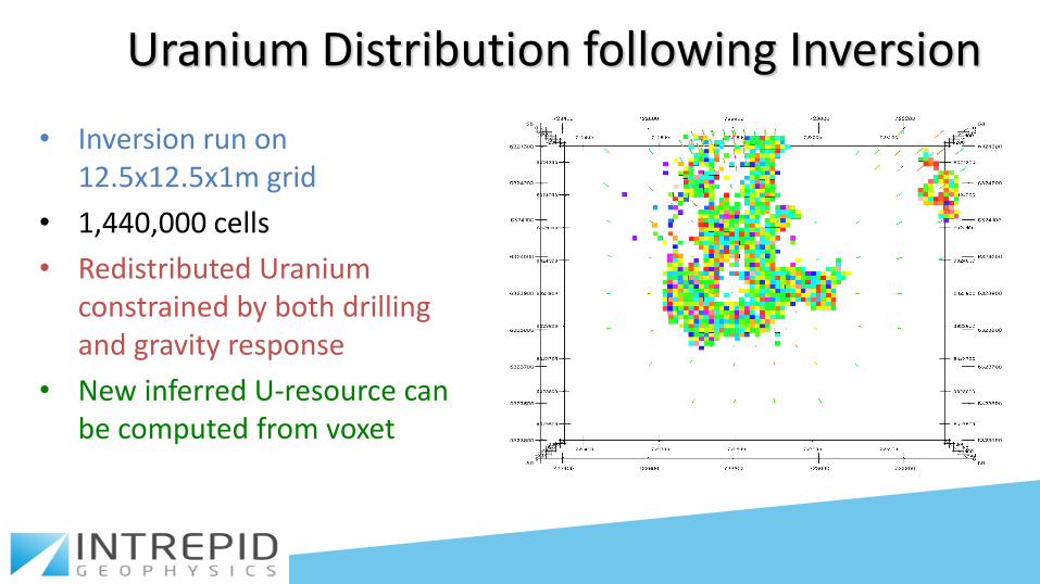
Uranium Distribution following Inversion

• Inversion run on 12.5x12.5x1m grid

• 1,440,000 cells

• Redistributed Uranium constrained by both drilling and gravity response

• New inferred U-resource can be computed from voxet

Conclusions and Recommendations

• Using Geostatistical Interpolation from Drilling logs to construct 3D property models is a powerful aid to constrained inversion

• Relations of measured physical properties and geochemistry need to be routinely logged and compared!!!!

• Initial Model is Driving Constraint

• Physical property model may imply the lithology

• USE your drilling logs!!!

Acknowledgments

• Thanks to Tullow Oil, Uranium SA and Intrepid Geophysics for permission to publish these studies

• Thankyou for your attention!!!

• www.intrepid-geophysics.com