Strategies for Constrained Optimisation 9

STRATEGIES FOR CONSTRAINED OPTIMISATION

G. M cC. Haworth1

Reading, England

ABSTRACT

The latest 6-man chess endgame results confirm that there are many deep forced mates beyond the 50-move rule. Players with potential wins near this limit naturally want to avoid a claim for a draw: optimal play to current metrics does not guarantee feasible wins or maximise the chances of winning against fallible opposition. A new metric and further strategies are defined which support players’ aspirations and improve their prospects of securing wins in the context of a k-move rule.

1. INTRODUCTION Endgame tables (EGTs) have to date not acknowledged the FIDE 50-move rule of Article 9.3. It is irrelevant for all but 8 of the 3- to 5-man endgames. Further, EGT authors share an interest with chess composers in the absolute capabilities of the chessmen. They have reasonably not given priority to FIDE’s flexible rule which has indeed changed five times (see below) and whose detail has been difficult to implement. However, recent progress on 6-man endgames (Nalimov, Wirth and Haworth, 1999; Hyatt, 2000; Karrer, 2000; Tamplin, 2000; Thompson, 2000) has renewed interest in having endgame data which serves both the practical player and the theoretician. The deeper maximum-depth wins imply that the 50-move rule will become a more frequent consideration. Let a won position be termed a k-win if k is the least integer for which optimal play would not risk a draw claim under a k-move rule. About half of the 6-man endgames computed to date feature k-wins with k > 50. Currently, practical players may be said to have two objectives:

• to win positions which are k-wins for k ≤ 50 without risking a 50-move draw claim, and • to maximise the probability of winning a k-win position for k > 50.

These objectives are addressed here. Section 2 questions the appropriateness of the rule given a demonstrably effective aggressor. Section 3 introduces a number of metrics that define varieties of optimal play. Section 4 shows the value of the now disused metric Depth to Zeroing move2 (DTZ). Section 5 defines the new metric Depth by the Rule (DTR) and describes algorithms for generating DTR data. Section 6 demonstrates the fail-ings of a naive strategy for using DTR and defines further strategies using DTR and DTZ data. 2. HISTORY OF THE RULE Ruy López suggested a 50-move limit in Article 17 of his Chess Code of 1561, perhaps in the interests of his fellow coffee-house professionals who played for wagers. The 1883 London Tournament’s rules, the basis of FIDE’s rules today, were the first to state that a P-push or capture would zero the count. In 1974, FIDE first enabled the 50-move rule to be varied. They did so with 100-move clauses, in 1978 for KNNKP (Troitzkiĭ, 1906-1910, 1934), in 1982 for KRP(a2)KbBP(a3) following the Timman-Velimirović game (Van den Herik, Herschberg and Nakad, 1987), and in 1984 for KRBKR (59) (Croskill, 1864; Nunn, 1994). They did not meet all the requirements defined by Roycroft (1984) at the first opportunity. By 1988, computer results, albeit single-sourced, were plentiful (Thompson, 1986) and endgame-specific limits were suggested. However, FIDE adopted a simpler stance, replacing the 100-move clauses by a 75-move al-lowance for just the six endgames KBBKN (Roycroft, 1983), KNNKP, KQKBB, KQKNN, KQP(x7)KQ and KRBKR (Kažíc, 1989; Mednis, 1989). KRPKBP with blocked Pawns ceased to be an exception. 1 ICL, Sutton’s Park Avenue, Sutton’s Park, Reading, Berkshire, RG6 1AZ, UK: guy.haworth@icl.com 2 A zeroing move is defined as one which zeroes the move count by FIDE Article 9.3, i.e., a pawn push, capture or mate. A phase of play is defined as a sequence of moves starting just after and ending with a zeroing move.

ICGA Journal March 2000 10

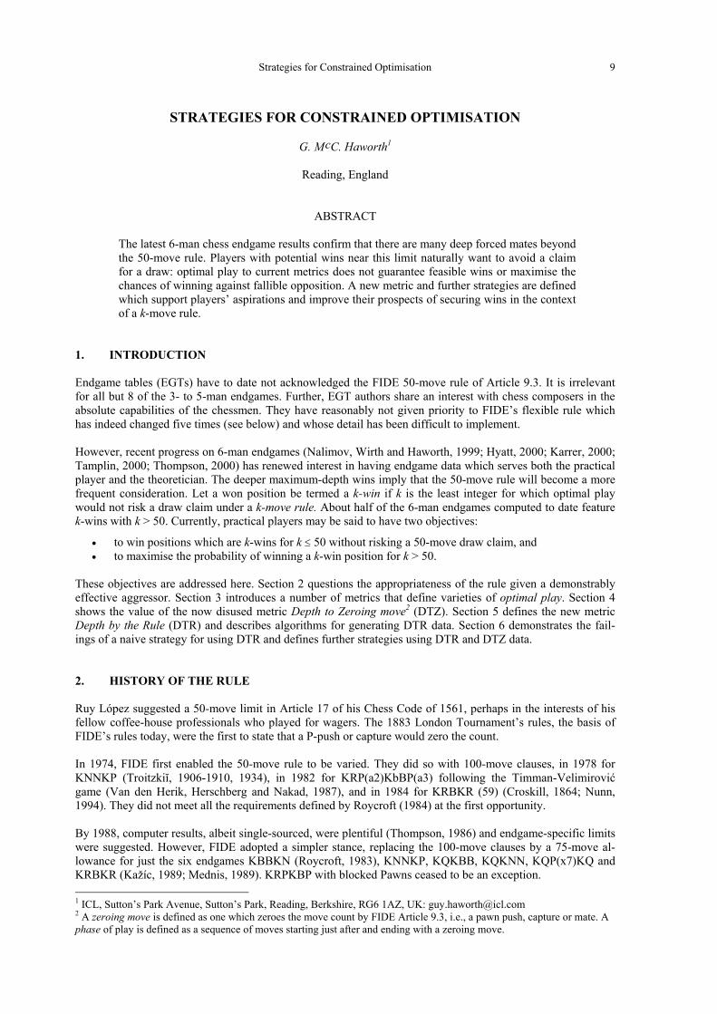
Following Stiller’s (1991) discovery that KRBKNN’s maximum depth is 223, FIDE gave up the chase and re-stored the 50-move limit for all endgames in 1992 (Herschberg and Van den Herik, 1993). KRNKNN then took the record phase length to 243 (Stiller, 1996) and this could well be extended by 7-man pawnless endgames. More details of some games and studies associated with the 50-move rule are in Appendix B. Clearly a balance has to be struck between the extremes of denying players attainable wins and requiring the opposition to be eternally vigilent in a drawn position. Today, the main concerns are social ones for the welfare of defenders and tournament directors who wish to run their events to a schedule (Levy and Newborn, 1991): however, it is clear that these need not apply to computer-assisted play. There is an argument for waiving the 50-move rule where a player can demonstrably achieve a theoretical win. An EGT is currently the only way to establish theoretical position values and benchmark the aggressor’s effectiveness. Certainly, computers with EGTs can play won or drawn positions quickly, even if they initially assume a fallible opponent and take time to choose between equi-optimal moves (Levy, 1991). Other means of winning effectively may be created in the future. To deny players the opportunity of achieving complex wins foreshortens the domain of chess itself. It prevents us from seeing immaculate play building on the smallest of advantages and exploring the deep space of the endgame where humans may never go without the vehicle of perfect information. 3. METRICS FOR OPTIMALITY Table 1 refines a previously published version (Nalimov et al., 1999) and contains a systematic notation to de-scribe the various optimisation goals and related concepts. It provides a way of referring to and comparing dif-ferent metrics, position depths, endgame tables, maximal depths, types of optimality and minimax strategies. Each strategy selects a subset of equi-optimal moves: one strategy may win where another draws. The actual line of play is determined by both sides’ respective strategies and their ultimate choice of equi-optimal moves.

Goal GZ GC GM GRZero 'Conversion', i.e., mate, Mate Mate within

Goal Description move-count capture or P-conversion in k -move rule ...in maximin in maximin maximin with

no. of moves no. of moves no. of moves maximin kReference player PZ PC PM PRMetric DTZ DTC DTM DTRPosition depth dz, dzi dc, dci dm, dmi dr, dri

Endgame Table EZ EC EM ERMaximal depth mxZ mxC mxM mxRType of optimality Z-optimal C-optimal M-optimal R-optimalMinimax Strategy ... move-subset chosen SZ SC SM SRExample EG tables by: Thompson (1986) KxPKx, x = Q, R 5-man 3- & 4-man 3-man Tamplin (2000); Thompson (2000) none 5- & 6-man 3- & 4-man 3-man Stiller (1989, 1991, 1992, 1996) none 5- & 6-man none none Hyatt (2000); Nalimov (2000) none none 3- to 6-man 3-man Wirth (1999) none KPPKP, KQQKQQ 3- & 4-man 3-man

Table 1: Endgame goals and associated concepts.

For pawnless endgames, DTC ≡ DTZ and SC ≡ SZ. The notation allows for more comprehensive goals. Let the nested strategy SX1X2...Xn be defined as subsetting the available moves with strategies SX1, SX2, ... , SXn in turn. A line X-Y is an optimal line of play where White is reference player PX using strategy SX and Black is reference player PY using strategy SY. Appendix A shows Black, then White, having to choose between C- and M-optimal play as they approach the events of force conversion and mate. For a specific k-win position P, a strategy SY is said to (k-)succeed on P if each move chosen by SY avoids the risk of a k-move draw claim. If not, SY (k-)fails on P and SY risks a draw claim on any positions from which Y-optimal play can arrive at P. Let σ denote any move-subsetting strategy. If SY succeeds on P, SYσ succeeds on P. However, as position Q-NN2 of Table 2 demonstrates, if SYσ succeeds on P, SY may still fail. Let SA ≥ SB denote that if strategy SA fails, strategy SB fails; SYσ ≥ SY. Let SA > SB denote that SA ≥ SB and that SA sometimes succeeds where SB fails.

Strategies for Constrained Optimisation 11

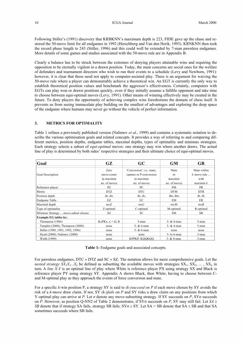
Key Position stm Val. DTZ DTC DTM DTR Notes ply ply ply ply

Maximal PositionsmxNN-P1 6N1/8/7p/8/8/8/3N1k2/7K w 1-0 ? 228 229 ? (Dekker, 1990). max DTM pos. ... 24. ... h4 {NN-P2}mxQ-NN 7Q/8/8/8/4n3/2k5/8/3K3n b 1-0 126 126 144 126 (Nunn, 1994, p. 307). ... 14. ... Kc6 {Q-NN1}mxQP-Q1 8/q7/P6k/Q7/8/8/8/6K1 w 1-0 141 213 235 141 (Thompson, 1986, p. 138). max DTZ wtm KQPKQ winmxRN-NN 6N1/5KR1/2n5/8/8/8/2n5/1k6 w 1-0 485 485 523 485 (Thompson, 2000). max DTC/DTM wtm KRNKNN win

Positions to test strategiesNN-P2 8/8/4k3/8/7p/6KN/6N1/8 w 1-0 ? 180 181 ? h3 needed before move 75. ... 62. ... Ke1 {NN-P3}NN-P3 8/8/8/8/7p/1N1K4/7N/4k3 w 1-0 ≤ 24 104 105 ? SZ succeeds; SC, SM fail with 63. Nd2 {NN-P4}NN-P4 8/8/8/8/7p/3K4/3N3N/4k3 b '1-0' 35 103 104 ? 63. .. Kf2 forces h3 to at least m80 and a draw claimQP-Q2 8/8/P7/6k1/3q4/8/4Q1K1/8 w 1-0 99 171 193 99 (Thompson, 1986, p. 138 after 21. ... Qd4)QP-Q3 K7/7k/P7/8/6q1/2Q5/8/8 w 1-0 1 17 41 ? (Thompson, 1986, p. 138 after 70. ... Kh7)

QBB-N1 6Q1/8/8/1n6/8/7K/7B/k6B w 1-0 2 2 7 5 PM-PM: 1. Be5+ Nd4 2. Bxd4 Kb1 3. Qb3+ Kc1 4. Be3#.QBB-N2 8/8/8/1n6/8/7K/k6B/7B w 1-0 103 103 127 103 {QBB-N1} PC-PC: 1. Qa2+ Kxa2 {QBB-N2}Q-NN1 8/8/2k5/8/4n3/3Q2n1/8/4K3 w 1-0 99 99 117 99 PMC-PCM: 1. Qd4 ... to 37. ... Ka4 {Q-NN2}Q-NN2 8/8/1n1K4/n1Q5/k7/8/8/8 w 1-0 25 25 41 25 SC, SMC succeed with Qg1; SM fails with Qc3/Qf2/Qg1

MiscellaneousNN-P5 7k/5K2/8/4N1N1/8/8/7p/8 b 1-0 1 1 2 1 The defender is forced to effect the conversion

Table 2: Illustrative chess positions.

4. ENDGAMES DEEPER THAN 50 MOVES Below is a list of known endgames with k-wins for k > 50 (Thompson, 1986, 2000; Van den Herik et al., 1987; Stiller, 1989, 1991, 1992, 1996; Dekker, Van den Herik and Herschberg, 1990; Wirth, 1999; Hyatt, 2000; Lin-cke, 2000; Nalimov, 2000; Tamplin, 2000). Obtrusive forces are in italics: mxR is in brackets.

5 man KBBKN (66), KBNKN (77), KNNKP (70+), KQKBB (71), KQKNN (63), KQRKQ (60), KRBKR (59), KQPKQ with wP on a6 (71), a7 (69), b3 (51), b6 (61), b7 (55), c3 (53), d3 (54), d4 (64), d6 (58).

6 man KBBBKR (69), KBBNKR (68), KNNNKB (92), KNNNKN (86), KQBKRR (85), KQKBBB (51+), KQKBBN (63+), KQNKRR (153), KQNNKQ (72), KQRKQB (73), KQRKQN (71), KQRKQR (92), KRBKBB (83), KRBKBN (98), KRBKNN (223), KRBNKQ (99), KRNKBB (140), KRNKBN (190), KRNKNN (243), KRP(a2)KbBP(a3) (54+), KRRBKQ (82), KRRKRB (54), KRRKRN (73), KRRNKQ (101), KRRRKQ (65).

Zeroing move, Conversion and Mate are increasingly distant goals. While the corresponding minimax strate-gies SZ, SC and SM are highly correlated, one strategy can preclude another. A focus on the longer-term objec-tives can extend the first phase beyond 50 moves but equally, an exclusive focus on the first phase can overextend a subsequent phase. In practice, players today have a choice only of tables providing DTC data (Thompson, 1986; ChessBase, 2000) or DTM data (Hyatt, 2000; Nalimov, 2000); no DTZ data is easily avail-able for P-endgames. Table 2, which collates all positions cited in this paper, gives examples of blind adher-ence to strategies SZ, SC or SM missing 50-wins, starting with three first-phase failures. The KQKNN position Q-NN1 (Tamplin, 2000) leads with MC-optimal play to position Q-NN2 on move 38. With just 13 moves left and all required for conversion, strategy SM selects 38. Qc3, Qf2 and Qg1 of which only Qg1 is C-optimal: SM therefore fails. Strategy SMC succeeds by narrowing the choice to Qg1. The maximal KNNKP position mxNN-P1 (Dekker, Van den Herik and Herschberg, 1990) leads by MC-CM play to NN-P2 after 24. ... h4. White must now force h3 by move 74. However, at position NN-P3, the SC and SM strategies dictate 63. Nd2 leading to position NN-P4. This allows 63. ... Kf2, postponing h3 until move 80. Strategies SC and SM therefore fail but Dekker et al. imply that strategy SZ forces h3 in time to win NN-P3. The KQPKQ position QP-Q3 is the result of 49 moves of Z-optimal play from QP-Q2 (Thompson, 1986, p. 138 after 21. ... Qd4) but could equally well have been the result of 49 moves of C-optimal play from another position. Strategy SZ succeeds just in time with 50. a7 but SC and SM fail by dictating 50. Kb8. The KQBBKN position QBB-N1 shows that strategy SZ, far from being a panacea, also fails. It misses the four-move mate, sacrifices the Queen unnecessarily and leaves a second phase of 52 moves. Perhaps one should never resign against a computer. Line f of Appendix A features a more benign knight sacrifice.

ICGA Journal March 2000 12

The positions above show SM, SC and SZ failing individually. However, with mleft denoting the number of moves left in the current phase, the following non-minimax strategies optimise against longer-term goals but safeguard the length of the current phase. They are defined in terms of the subset of moves they return:

SZ' ≡ {move to P(dzi) | dzi ≤ mleft - 1} Sσ* ≡ if dz > mleft then SZ else SZ'σ .. e.g., SC*, SM* and SMC* ≡ (SMC)*. Sσ* ≥ Sσ but SZσ* ≡ SZσ. SA1 ≡ if dm ≤ mleft then SM else if dc ≤ mleft then SC else SZCM.

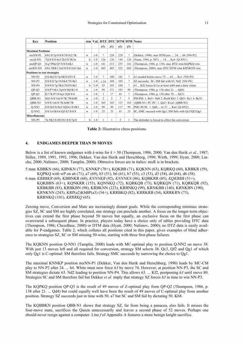
SM* and SA1 succeed on the positions above but it is conjectured that they fail to win some winnable positions and that a metric recognising a k-move rule explicitly is needed. For example, KBBKNN has mxM = 106 moves and mxZ = 38 moves (Stiller, 1996); 24% of wtm positions are wins and 65% of these have dm > 50. It converts to KBBKN which has dz > 50 for some 11.16% of White wins. Let the KBBKN wins for White be partitioned into sets W (dz ≤ 50) and D (dz > 50). Let three subsets of KBBKNN wins be defined as follows:

A ≡ {P | P is a Wh. win: Wh. cannot mate in KBBKNN but can force P to Pw ∈ W in dzw ≤ 50 moves} B ≡ {P | P is a Wh. win: Wh. cannot mate in KBBKNN but can force P to Pd ∈ D in dzd ≤ 50 moves} AB ≡ {P | P ∈ A ∩ B, dm > 50 and dzd ≤ dzw implying dz = dzd ≤ 50}, see Figure 1.

dzd DTC = 50 dzw

KBBKNN KBBKN

KBBK

DW

P SM*: dm > 50

B AB

Draw Claim

Draw Claim or Win?

WinPw

Pd

A

Figure 1: Winning a ‘difficult’ position P in KBBKNN.

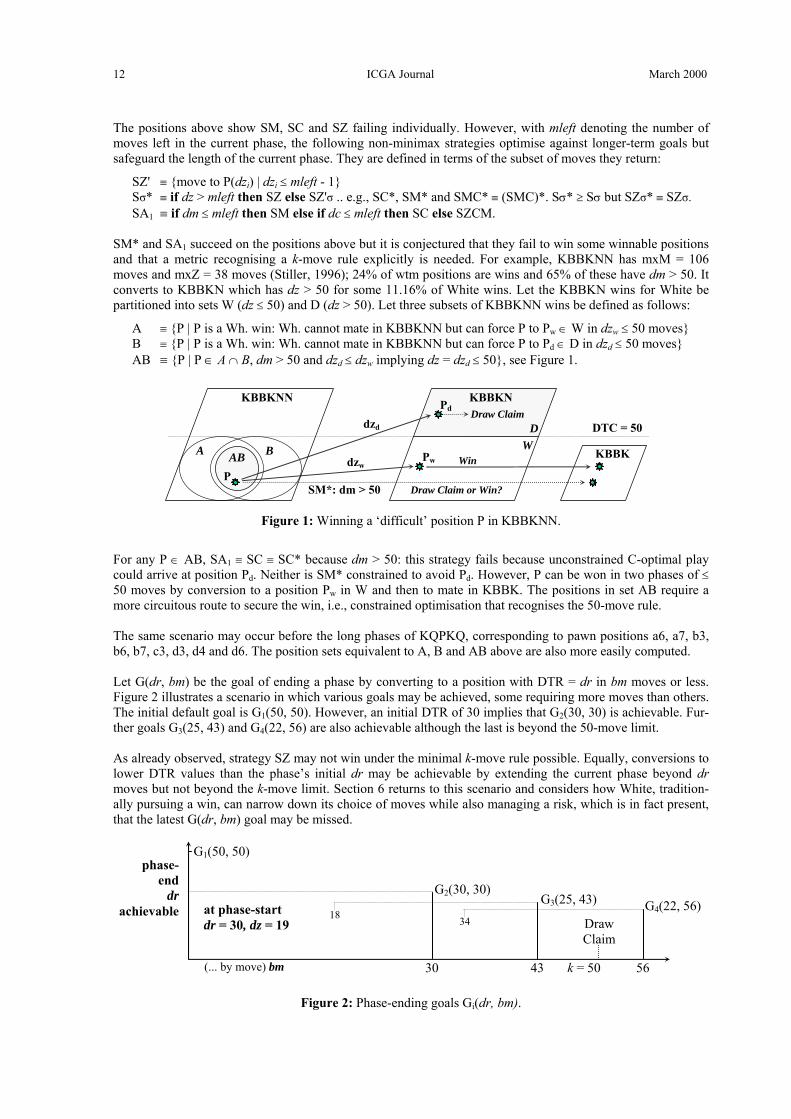
For any P ∈ AB, SA1 ≡ SC ≡ SC* because dm > 50: this strategy fails because unconstrained C-optimal play could arrive at position Pd. Neither is SM* constrained to avoid Pd. However, P can be won in two phases of ≤ 50 moves by conversion to a position Pw in W and then to mate in KBBK. The positions in set AB require a more circuitous route to secure the win, i.e., constrained optimisation that recognises the 50-move rule. The same scenario may occur before the long phases of KQPKQ, corresponding to pawn positions a6, a7, b3, b6, b7, c3, d3, d4 and d6. The position sets equivalent to A, B and AB above are also more easily computed. Let G(dr, bm) be the goal of ending a phase by converting to a position with DTR = dr in bm moves or less. Figure 2 illustrates a scenario in which various goals may be achieved, some requiring more moves than others. The initial default goal is G1(50, 50). However, an initial DTR of 30 implies that G2(30, 30) is achievable. Fur-ther goals G3(25, 43) and G4(22, 56) are also achievable although the last is beyond the 50-move limit.

As already observed, strategy SZ may not win under the minimal k-move rule possible. Equally, conversions to lower DTR values than the phase’s initial dr may be achievable by extending the current phase beyond dr moves but not beyond the k-move limit. Section 6 returns to this scenario and considers how White, tradition-ally pursuing a win, can narrow down its choice of moves while also managing a risk, which is in fact present, that the latest G(dr, bm) goal may be missed. G1(50, 50)

30 43 56

G4(22, 56) G3(25, 43) G2(30, 30)

3418at phase-start dr = 30, dz = 19

(... by move) bm 50 k =

Draw Claim

phase- end

dr achievable

Figure 2: Phase-ending goals Gi(dr, bm).

Strategies for Constrained Optimisation 13

5. THE DTR METRIC AND ENDGAME TABLE The 50-move rule generalises to the k-move rule and suggests metric DTR as follows:

a position’s Depth by the Rule, DTR, is the least k for which the position can be won without the risk of a draw claim under a k-move rule.

It immediately follows that dz ≤ dc ≤ dm, dz ≤ dr ≤ dm, and that a position can be moved to the next phase in at most a further dr moves, leaving a position with DTR ≤ dr. Further, a position’s dr satisfies:

• dr = max [dz, min (dr of won successors)] for side-to-move, stm, wins • dr = max [dz, max (dr of lost successors)] for stm losses

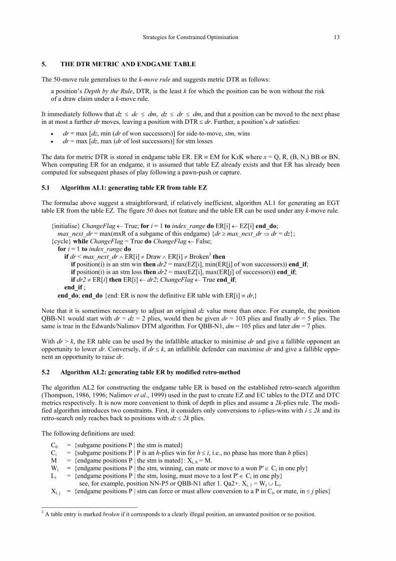
The data for metric DTR is stored in endgame table ER. ER ≡ EM for KxK where x = Q, R, (B, N,) BB or BN. When computing ER for an endgame, it is assumed that table EZ already exists and that ER has already been computed for subsequent phases of play following a pawn-push or capture. 5.1 Algorithm AL1: generating table ER from table EZ The formulae above suggest a straightforward, if relatively inefficient, algorithm AL1 for generating an EGT table ER from the table EZ. The figure 50 does not feature and the table ER can be used under any k-move rule.

{initialise} ChangeFlag ← True; for i = 1 to index_range do ER[i] ← EZ[i] end_do; max_next_dr = max(mxR of a subgame of this endgame) {dr ≥ max_next_dr ⇒ dr = dz}; {cycle} while ChangeFlag = True do ChangeFlag ← False; for i = 1 to index_range do if dr < max_next_dr ∧ ER[i] ≠ Draw ∧ ER[i] ≠ Broken3 then if position(i) is an stm win then dr2 = max(EZ[i], min(ER[j] of won successors)) end_if; if position(i) is an stm loss then dr2 = max(EZ[i], max(ER[j] of successors)) end_if; if dr2 ≠ ER[i] then ER[i] ← dr2; ChangeFlag ← True end_if; end_if ; end_do; end_do {end: ER is now the definitive ER table with ER[i] ≡ dri}

Note that it is sometimes necessary to adjust an original dz value more than once. For example, the position QBB-N1 would start with dr = dz = 2 plies, would then be given dr = 103 plies and finally dr = 5 plies. The same is true in the Edwards/Nalimov DTM algorithm. For QBB-N1, dm = 105 plies and later dm = 7 plies. With dr > k, the ER table can be used by the infallible attacker to minimise dr and give a fallible opponent an opportunity to lower dr. Conversely, if dr ≤ k, an infallible defender can maximise dr and give a fallible oppo-nent an opportunity to raise dr. 5.2 Algorithm AL2: generating table ER by modified retro-method The algorithm AL2 for constructing the endgame table ER is based on the established retro-search algorithm (Thompson, 1986, 1996; Nalimov et al., 1999) used in the past to create EZ and EC tables to the DTZ and DTC metrics respectively. It is now more convenient to think of depth in plies and assume a 2k-plies rule. The modi-fied algorithm introduces two constraints. First, it considers only conversions to i-plies-wins with i ≤ 2k and its retro-search only reaches back to positions with dz ≤ 2k plies. The following definitions are used:

C0 = {subgame positions P | the stm is mated} Ci = {subgame positions P | P is an h-plies win for h ≤ i, i.e., no phase has more than h plies} M = {endgame positions P | the stm is mated}: Xi, 0 = M. Wi = {endgame positions P | the stm, winning, can mate or move to a won P' ∈ Ci in one ply} Li = {endgame positions P | the stm, losing, must move to a lost P' ∈ Ci in one ply} see, for example, position NN-P5 or QBB-N1 after 1. Qa2+. Xi, 1 = Wi ∪ Li. Xi, j = {endgame positions P | stm can force or must allow conversion to a P in Ci, or mate, in ≤ j plies}

3 A table entry is marked broken if it corresponds to a clearly illegal position, an unwanted position or no position.

ICGA Journal March 2000 14

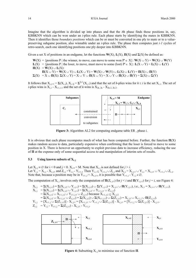
Imagine that the algorithm is divided up into phases and that the ith phase finds those positions in, say, KBBKNN which can be won under an i-plies rule. Each phase starts by identifying the mates in KBBKNN. Then it identifies those boundary positions which can be or must be converted in one ply to mate or to a value-preserving subgame position, also winnable under an i-plies rule. The phase then computes just i-1 cycles of retro-search, each one identifying positions one ply deeper into KBBKNN. Given a set X of positions in an endgame, let the functions W(X), L(X), Π(X) and Σ(X) be defined as:

W(X) = {positions P | the winner, to move, can move to some won P' ∈ X}: W(X ∪ Y) = W(X) ∪ W(Y) L(X) = {positions P | the loser, to move, must move to some (lost) P' ∈ X}: L(X ∪ Y) = L(X) ∪ L(Y) Π(X) = W(X) ∪ L(X): Π(X ∪ Y) = W(X ∪ Y) ∪ L(X ∪ Y) = W(X) ∪ W(Y) ∪ L(X) ∪ L(Y) = Π(X) ∪ Π(Y) Σ(X) = X ∪ Π(X): Σ(X ∪ Y) = X ∪ Y ∪ Π(X ∪ Y) = X ∪ Y ∪ Π(X) ∪ Π(Y) = Σ(X) ∪ Σ(Y)

It follows that Xi, j+1 = Σ(Xi, j), Xi, 2j = Σ2j-1(Xi, 1) and that the set of h-plies wins for h ≤ i is the set Xi, i. The set of i-plies wins is Xi, i - Xi-1, i-1 and the set of k-wins is X2k, 2k - X2k-2, 2k-2.

Figure 3: Algorithm AL2 for computing endgame table ER , phase i.

It is obvious that each phase recomputes much of what has been computed before. Further, the function Π(X) makes random access to data, particularly expensive when confirming that the loser is forced to move to some position in X. There is however an opportunity to exploit previous data to increase efficiency, reducing the use of Π at the expense only of some sequential access to and manipulation of interim sets of results. 5.3 Using known subsets of Xi, j Let Xi, j ≡ ∅ for i < 0 and j < 0. Xi, 0 = M. Note that Xi, j is not defined for j > i. Let Yi, j = Xi, j - Xi, j-1 and Zi, j =Yi, j - Yi-1, j. Then Yi, j ⊆ Yi-1, j ∪ Zi, j and Xi, j = Xi, j-1 ∪ Yi, j = Xi, j-1 ∪ Yi-1, j ∪ Zi, j. Note that, because a position may be in Yi-1, j ∩ Xi, j-1, it is possible that Yi-1, j - Yi, j ≠ ∅.

The computation of Xi, j involves only the computation of Π(Zi, j-1) for j < i and Π(Yi, j-1) for j = i, see Figure 4:

Xi, j = Σ(Xi, j-1) = Σ(Xi, j-2 ∪ Yi, j-1) = Σ(Xi, j-2) ∪ Σ(Yi, j-1) = Xi, j-1 ∪ Π(Yi, j-1), i.e., Xi, i = Xi, i-1 ∪ Π(Yi, i-1). Xi, j = Σ(Xi, j-1) = Σ(Xi, j-2 ∪ Yi, j-1) = Σ(Xi, j-2 ∪ Yi-1, j-1 ∪ Zi, j-1) = Σ(Xi, j-2 ∪ Xi-1, j-2 ∪ Yi-1, j-1 ∪ Zi, j-1) because Xi-1, j-2 ⊆ Xi, j-2 = Σ(Xi, j-2 ∪ Xi-1, j-1 ∪ Zi, j-1) = Σ(Xi, j-2) ∪ Σ(Xi-1, j-1) ∪ Σ(Zi, j-1) = Xi, j-1 ∪ Xi-1, j ∪ Π(Zi, j-1). Yi, j = [Xi-1, j ∪ Σ(Zi, j-1)] - Xi, j-1 = [Xi-1, j-1 ∪ Yi-1, j ∪ Σ(Zi, j-1)] - Xi, j-1 = [Yi-1, j ∪ Σ(Zi, j-1)] - Xi, j-1. Zi, j = Yi, j - Yi-1, j = Σ(Zi, j-1) - Xi, j-1 - Yi-1, j.

Xi-1, j

Zi, j-1Π Xi, j

Π

Xi, i-2

Ci

Subgames

Π

Endgame

Xi, 1 = Wi ∪ Li ∪ Xi, 0

Xi, 0 = M

Xi, i

to subgames

conversion

constrained

Xi, j-1

Xi, i

Xi, i-1

Yi, i-1

Figure 4: Subsetting Xi, j to minimise use of function Π.

Strategies for Constrained Optimisation 15

6. USES OF THE DTR DATA Let us suppose, as is usual, that White is pursuing a win under a k-move rule against a possibly fallible player. For convenience, moves will be numbered from 1 in the current phase. The following notation is used:

k indicates the k-move rule in force: currently, FIDE has set k = 50 for all endgames mplayed the history factor, the number of white moves played in this phase mleft the number of white moves left before the risk of a draw claim; mleft = k - mplayed P(dr, dz) a wtm position P with depths dr in metric DTR and dz in metric DTZ CP the set {Pi(dri, dzi)} of btm successors of position P

CQ the subset {Pi ∈ CP | dzi ≤ mleft - 1}: ∅ ⊆ CQ ⊆ CP. Gj(drj , bmj) the jth goal, to conclude the phase by conversion with DTR drj on or before move bmj gi index of the last goal defined

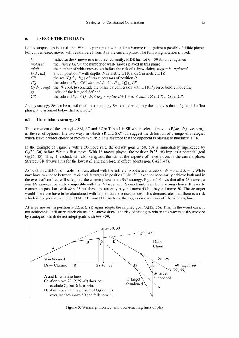
CR the subset {Pi ∈ CQ | dri ≤ drgi ∧ mplayed + 1 + dzi ≤ bmgi}: ∅ ⊆ CR ⊆ CQ ⊆ CP. As any strategy Sσ can be transformed into a strategy Sσ* considering only those moves that safeguard the first phase, it is assumed below that dz ≤ mleft. 6.1 The minimax strategy SR The equivalent of the strategies SM, SC and SZ in Table 1 is SR which selects {move to Pi(dri, dzi) | dri ≤ drj} as the set of options. The two ways in which SR and SR* fail suggest the definition of a range of strategies which leave a wider choice of moves available. It is assumed that the opponent is playing to maximise DTR. In the example of Figure 2 with a 50-move rule, the default goal G1(50, 50) is immediately superceded by G2(30, 30) before White’s first move. With 18 moves played, the position P(25, dz) implies a potential goal G3(25, 43). This, if reached, will also safeguard the win at the expense of more moves in the current phase. Strategy SR always aims for the lowest dr and therefore, in effect, adopts goal G3(25, 43). As position QBB-N1 of Table 1 shows, albeit with the entirely hypothetical targets of dr = 3 and dz = 1, White may have to choose between its dr and dz targets in position P(dr, dz). It cannot necessarily achieve both and in the event of conflict, will safeguard the current phase in an Sσ* strategy. Figure 5 shows that after 28 moves, a feasible move, apparently compatible with the dr target and dz constraint, is in fact a wrong choice. It leads to conversion positions with dr ≤ 25 but these are not only beyond move 43 but beyond move 50. The dr target would therefore have to be abandoned with unpredictable consequences. This demonstrates that there is a risk which is not present with the DTM, DTC and DTZ metrics: the aggressor may stray off the winning line. After 33 moves, in position P(22, dz), SR again adopts the implied goal G4(22, 56). This, in the worst case, is not achievable until after Black claims a 50-move draw. The risk of failing to win in this way is easily avoided by strategies which do not adopt goals with bm > 50.

G2(30, 30)

D C A

A and B: winning lines C: after move 28, P(25, dz) does not exclude G3 but fails to win. D: after move 33, the pursuit of G4(22, 56) over-reaches move 50 and fails to win.

B

Draw Claimed Win Secured

Draw Claim

G3(25, 43)

333018 28 50 60 43

dr target abandoned

53 56

mplayed

dr target abandoned

G4(22, 56)

Figure 5: Winning, incorrect and over-reaching lines of play.

ICGA Journal March 2000 16

The following measures are suggested to lower the residual risk of a draw claim when using SR*:

• avoid subsetting the moves offered by SR*, e.g., by minimum dz • instead, search forward a number of plies continuing to subset options with SR* • if the lowest visible dr in unattainable within k moves, relax the dr goal.

Given the failings of SR*, a range of strategies SRa is defined, featuring constraints on the dr attempted. 6.2 The SRa Strategies Four strategies are defined differing in the criteria applied to potential goals before they are adopted as actual goals. All strategies adopt the default goal G1(k, k) in the context of a k -move rule, even though it might not be achievable against infallible play. SR* above is equivalent to SR4* below. In summary:

• SR1 focuses only on goal G1(k, k), in effect, providing a fixed filter on the move options • SR2, given goal Gi(dri, bmi), adopts Gj(drj, bmj) provided drj < dri and bmj ≤ bmi: SR2 ≥ SR1 • SR3, given goal Gi(dri, bmi), adopts Gj(drj, bmj) provided drj < dri and bmj ≤ k: SR3 ≥ SR1 • SR4, given goal Gi(dri, bmi), adopts Gj(drj, bmj) provided drj < dri.

Where SR2 and SR3 adopt a new goal, they confirm that the aggressor has a winning line and the effect of any previous, suboptimal choices of move may be ignored. Returning to the example of Figure 2, SR1 uses only goal G1, SR2 uses G1 and G2, SR3 uses G1-G3 and SR4 uses G1-G4. 6.3 An algorithm for the SRa The algorithm, written for the attacker, returns a subset CM of moves. To guard against DTR > k, CM is first defined to be the same subset which strategy SR will return, i.e., those moves with minimal dr.

{initialise: a ≡ dr_focus is assumed set} high_value = 109; if mplayed = 0 then G1 ← G1(k, k); gi ← 1 end_if; {step 1: in case dr > k} CM ← {Pi | Pi is selected by strategy SR} {step 2: re-adopt a previous goal if this exists and the current goal is clearly unattainable} while CR = ∅ ∧ gi > 1 do gi ← gi - 1; {step 3: if possible, set a stronger goal from those implied by the current move options}

if a ≠ 1 ∧ CR ≠ ∅ then drmin = min{dri | Pi(dri, dzi) ∈ CR};

if mplayed + 1 + drmin ≤ bm_limit(a) then add_new_goal(G, gi) end_if end_if;

{step 4: if possible, subset to Pi not excluding the current goal} if CR ≠ ∅ then CM ← CR;

where bm_limit(a) ≡ begin if a = 1, 2, 3 or 4 then k, bmgi, k or high_value respectively end_if and add_new_goal(G, gi, ...) ≡ begin gi ← gi + 1; Ggi = Ggi(drmin, drmin + mplayed + 1) end 6.4 Examples of SRa in use SR1 succeeds where SZ fails on position QBB-N1 of Table 1 and positions P ∈ AB in Figure 1. Strategy SA1 of section 4 can be strengthened to:

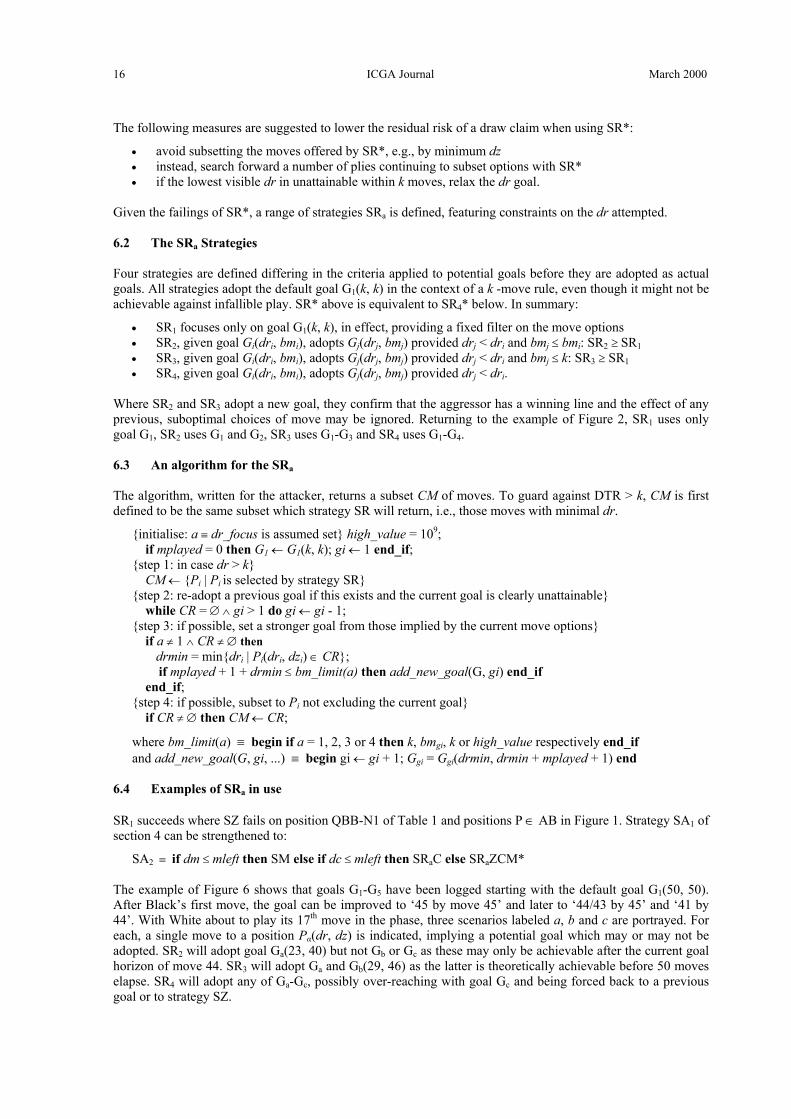
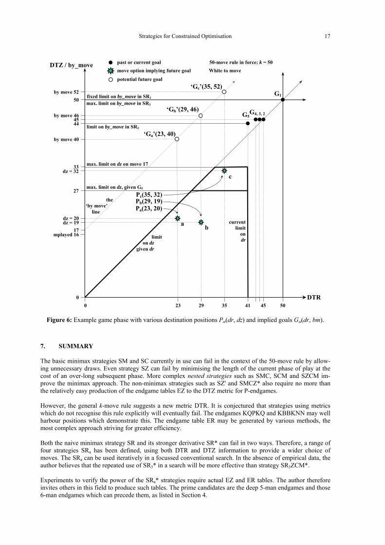
SA2 ≡ if dm ≤ mleft then SM else if dc ≤ mleft then SRaC else SRaZCM* The example of Figure 6 shows that goals G1-G5 have been logged starting with the default goal G1(50, 50). After Black’s first move, the goal can be improved to ‘45 by move 45’ and later to ‘44/43 by 45’ and ‘41 by 44’. With White about to play its 17th move in the phase, three scenarios labeled a, b and c are portrayed. For each, a single move to a position Pα(dr, dz) is indicated, implying a potential goal which may or may not be adopted. SR2 will adopt goal Ga(23, 40) but not Gb or Gc as these may only be achievable after the current goal horizon of move 44. SR3 will adopt Ga and Gb(29, 46) as the latter is theoretically achievable before 50 moves elapse. SR4 will adopt any of Ga-Gc, possibly over-reaching with goal Gc and being forced back to a previous goal or to strategy SZ.

Strategies for Constrained Optimisation 17

DTZ / by_move

27

50

by move 40

dz = 20

mplayed 16

45 by move 46

44

0

by move 52

dz = 32 33 max. limit on dz on move 17

the ‘by move’ .

line .

‘Ga’(23, 40)

‘Gb’(29, 46)

‘Gc’(35, 52)potential future goal

move option implying future goal

current limit

on dr

G1

G4, 3, 2G5

dz

Pa(23, 20)Pb(29, 19)Pc(35, 32)

White to move

limit on dz .

given dr .

max. limit on dz, given G5

max. limit on by_move in SR3

fixed limit on by_move in SR1

limit on by_move in SR2

a b

c

17 = 19

50-move rule in force; k = 50 past or current goal

DTR 0 23 29 35 41 45 50

Figure 6: Example game phase with various destination positions Pα(dr, dz) and implied goals Gα(dr, bm).

7. SUMMARY The basic minimax strategies SM and SC currently in use can fail in the context of the 50-move rule by allow-ing unnecessary draws. Even strategy SZ can fail by minimising the length of the current phase of play at the cost of an over-long subsequent phase. More complex nested strategies such as SMC, SCM and SZCM im-prove the minimax approach. The non-minimax strategies such as SZ' and SMCZ* also require no more than the relatively easy production of the endgame tables EZ to the DTZ metric for P-endgames. However, the general k-move rule suggests a new metric DTR. It is conjectured that strategies using metrics which do not recognise this rule explicitly will eventually fail. The endgames KQPKQ and KBBKNN may well harbour positions which demonstrate this. The endgame table ER may be generated by various methods, the most complex approach striving for greater efficiency. Both the naive minimax strategy SR and its stronger derivative SR* can fail in two ways. Therefore, a range of four strategies SRa has been defined, using both DTR and DTZ information to provide a wider choice of moves. The SRa can be used iteratively in a focussed conventional search. In the absence of empirical data, the author believes that the repeated use of SR3* in a search will be more effective than strategy SR3ZCM*. Experiments to verify the power of the SRa* strategies require actual EZ and ER tables. The author therefore invites others in this field to produce such tables. The prime candidates are the deep 5-man endgames and those 6-man endgames which can precede them, as listed in Section 4.

ICGA Journal March 2000 18

8. ACKNOWLEDGMENTS First, my thanks to the authors of the endgame tables - Stephen Edwards, Eugene Nalimov, Lewis Stiller, Ken Thompson and Christoph Wirth. Experience to date confirms the accuracy and efficiency of these tables. My thanks also to Helmut Conrady, Peter Karrer, Tim Krabbé, Thomas Lincke, John Roycroft, John Tamplin and Ken Thompson for occasional dialogue. Finally, my thanks to the referees and editor for their particularly use-ful comments on the early drafts. 9. REFERENCES ChessBase (2000). http://www.chessbase.com/. CD publisher of Nalimov and Thompson endgame tables.

ChessLab (2000). http://chesslab.com/. Database of 2 million games dating from 1485.

Croskill (1864). The rook and bishop against rook. The Chess Player’s Magazine, Vol. 2, pp. 305-311.

Dekker, S.T., Herik, H.J. van den and Herschberg, I.S. (1990). Perfect Knowledge Revisited. Artificial Intelli-gence, Vol. 43, No. 1, pp. 111-123.

Herik, H.J. van den, Herschberg, I.S. and Nakad, N. (1987). A Six-Men-Endgame Database: KRP(a2)-KbBP(a3). ICCA Journal, Vol. 10, No. 4, pp. 163-180.

Herschberg, I.S. and Van den Herik, H.J. (1993). Back to Fifty. ICCA Journal, Vol. 16, No. 1, pp. 1-2.

Hyatt, R. (2000). ftp://ftp.cis.uab.edu/pub/hyatt/TB/. Server providing Nalimov’s EG statistics and tables.

Kažíc, B.M. (1989). The 50-Move Rule Adapted (2). ICCA Journal, Vol. 12, No. 2, p. 123.

Karrer, P (2000). KQQKQP and KQPKQP≈. ICGA Journal, Vol. 23, No. 2.

Levy, D. (1991). First among equals. ICCA Journal, Vol. 14, No. 3, p. 142.

Levy, D. and Newborn, M. (1991). How Computers Play Chess. Freeman & Co. ISBN 0-7167-8121-2 (pbk.), esp. pp. 128-152.

Lincke, T. (2000). http://wwwjn.inf.ethz.ch/games/chess/statistics/chs_statistics.html. DTC win and draw sta-tistics for 3-man to 6-man endgames.

Mednis, E. (1989). The 50-Move Rule Adapted (1). ICCA Journal, Vol. 12, No. 2, p. 123.

Nalimov, E.V., Wirth, C., and Haworth, G.McC. (1999). KQQKQQ and the Kasparov-World Game. ICCA Journal, Vol. 22, No. 4, pp. 195-212.

Nalimov, E.V. and Heinz, E.A. (2000). Space-Efficient Indexing of Endgame Databases for Chess. Advances in Computer Games 9, (eds. H. J. van den Herik and B. Monien). Institute for Knowledge and Agent Technology (IKAT), Maastricht, The Netherlands. To appear.

Nefkens, H.J.J. (1991). How to Win with a Knight Ahead. ICCA Journal, Vol. 14, No. 4, pp. 201-203.

Nunn, J. (1994). Secrets of Pawnless Endings. B.T. Batsford, London. ISBN 0-7134-7508-0.

Roycroft, A.J. (1983). A Prophecy Fulfilled. EG, Vol. V, No. 74, pp. 217-220.

Roycroft, A.J. (1984). A Proposed Revision of the ‘50-Move Rule’. ICCA Journal, Vol. 7, No. 3, pp. 164-170.

Roycroft, A.J. (1986). Adjudicate This!! EG, No. 83, p. 22.

Roycroft, A.J. (1988). Expert against the Oracle. Machine Intelligence 11 (eds. J.E. Hayes, D. Michie and J. Richards) pp. 347-373. Oxford University Press, Oxford. ISBN 0-1985-3718-2.

Stiller, L.B. (1989). Parallel Analysis of Certain Endgames. ICCA Journal, Vol. 12, No. 2, pp. 55-64.

Stiller, L.B. (1991). Some Results from a Massively Parallel Retrograde Analysis. ICCA Journal, Vol. 14, No. 3, pp. 129-134.

Stiller, L.B. (1991b). Karpov and Kasparov: the End is Perfection. ICCA Journal, Vol. 14, No. 4, pp. 198-201.

Stiller, L.B. (1992). KQNKRR. ICCA Journal, Vol. 15, No. 1, pp. 16-18.

Stiller, L.B. (1996). Multilinear Algebra and Chess Endgames. Games of No Chance (ed. R.J. Nowakowski), pp. 151-192. MSRI Publications, v29, CUP, Cambridge, England. ISBN 0-521-64652-9.

Strategies for Constrained Optimisation 19

Tamplin, J. (2000). http://chess.liveonthenet.com/chess/endings/index.shtml. Position evaluation via Karrer’s KQQKQP≈/KQPKQP≈ sub-EGTs, Nalimov’s 3-6-man EGTs and Thompson’s 5-man EGTs and maximals.

Thompson, K. (1986). Retrograde Analysis of Certain Endgames. ICCA Journal, Vol. 9, No. 3, pp. 131-139.

Thompson, K. (1996). 6-Piece Endgames. ICCA Journal, Vol. 19, No. 4, pp. 215-226.

Thompson, K. (2000). http://cm.bell-labs.com/cm/cs/who/ken/chesseg.html. 6-man EGT maximal positions, maximal mutual zugzwangs and endgame statistics.

Troitzkiĭ, A.A. (1906-1910) Serialised analysis of KNNKP. Deutsche Schachzeitung.

Troitzkiĭ, A.A. (1934). Два коня против пешек (теоретический очерк). Сборник шахматных этюдов, pp. 248-288. Leningrad. [Dva Konya protiv pešek. Sbornik šakhmatnykh étyudov.] Partly republished (1937) in Collection of Chess Studies, with a Supplement on the Theory of the End-Game of Two Knights against Pawns. (trans. A.D. Pritzson), David McKay Company, the latter again re-published (1985) by Olms, Zürich.

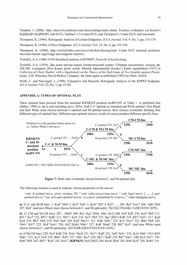
Wirth, C. and Nievergelt, J. (1999). Exhaustive and Heuristic Retrograde Analysis of the KPPKP Endgame. ICCA Journal, Vol. 22, No. 2, pp. 67-80. APPENDIX A: TYPES OF OPTIMAL PLAY These optimal lines proceed from the maximal KRNKNN position mxRN-NN of Table 1. A published line (Stiller, 1996) is, up to and including move 205w, both C-C optimal as intended and M-M optimal. First Black and then White must choose between C-optimal and M-optimal moves, their choices eventually defining four different types of optimal line. Different equi-optimal choices would of course produce different specific lines.

e

g

f

262b 239b MC-MC line

270b 239b CM-MC line

208w M-optimal 239. Kc64

239w

C-optimal 239. Nb62

C-MC & M-MC line

d

c

253b 229b MC-CM line

246b 229b CM-CM line

208w M-optimal 229. Rh1'

C-optimal 229. Na5'

229w C-CM & M-CM line

b

a1w

M-optimal 207. ... Nba6'

C-optimal 207. ... Nbd5'

207b C-C & M-M line

Position nw is the position before move nw i.e., before White’s nth move. KRNKNN C- and M- maximal position

mxRN-NN

mxRN-NN = 6N1/5KR1/2n5/8/8/8/2n5/1k6+w

Figure 7: Both sides eventually choose between C- and M-optimal play

The following notation is used to indicate various properties of the moves:

' only X-optimal move, given strategy SX; " only value-preserving move; ° only legal move; [..., ...] equi-optimal moves; n one of n equi-optimal moves; -n a move suboptimal by n moves; v value-changing move.

a) {C-C and M-M line} 1. Ke6" Nb4' 2. Ke5" Nd3' 3. Ke4" Nf2' 4. Kf3" ..... 205. Re5' Nec7' 206. Nd6' Nb4' 207. Re4' {and now Black must choose between C- and M-optimality: 5k2/2n5/3N4/6K1/1n2R3/8/8/8+207b}.

b) {C-CM and M-CM line} 207... Nbd5' 208. Re1' Kg7 [Nb4, Nb6, Nc3] 209. Kf5' Kf8' 210. Ke5' Nb4' 211. Rf1+' Ke7' 212. Rf7+' Kd8° 213. Nb7+' Kc8' 214. Nc5' Nb5' 215. Rg7 [Rh7] Kd8' 216. Rb7' Nc6+' 217. Ke6' Kc8' 218. Rh7' Nb4' 219. Na4' Na6' 220. Kd5' Nbc7+' 221. Kd6' Ne8+' 222. Ke7' Nec7' 223. Rh6' Nb8' 224. Nb6+' Kb7° 225. Nc4' Nc6+' 226. Kd7 [Kd6] Nb8+' 227. Kd6' Nba6' 228. Rh7' Kc8' {and now White must choose between C- and M-optimality: 2k5/2n4R/n2K4/8/2N5/8/8/8+229w}.

c) {CM-CM line} 229. Na5' Kd8' 230. Nc6+' Kc8' 231. Ne7+' Kd8' 232. Nd5' Ne8+' 233. Kc6' Nb8+' 234. Kb5' Nd6+' 235. Kc5' Nc8' 236. Rh8+' Kd7° 237. Nf6+' Kc7' 238. Rh7+' Kd8' 239. Rb7' Na6+' 240. Kc6' Ne7+' 241. Kb6' Nb4' 242. Rd7+' Kc8° 243. Rxe7' {KRNKN} Nc6 [Nd5] 244. Kxc6' Kb8' 245. Kb6' Kc82 246. Re8#' 1-0.

ICGA Journal March 2000 20

d) {MC-CM line} 229. Rh1' Kd8' 230. Rh8+' Ne8+° 231. Ke6' Nc7+' 232. Kf7' Kd7' 233. Rh6" Nd5' 234. Ne5+" Kd8' 235. Rh2' Ndc7' 236. Rh8' Kc8' 237. Rh6' Kd8' 238. Nc4' Kc8' 239. Rg6' Kb8' 240. Ke7' Kc8' 241. Ne3' Kb8' 242. Kd8' Kb72 243. Kd7 [Nc4] Kb83 244. Rb6+' Ka7' 245. Rb1' Ka62 246. Nc4' Ka7' 247. Rb2' Ka6' 248. Kc6' Ka7' 249. Nb6' Kb8' 250. Nd7+' Ka7' 251. Rb42 Ka82 252. Ra4+' Na6° 253. Rxa6#' {KRNKN} 1-0.

e) {C-MC and M-MC line} 207. ... Nba6' 208. Kf5' Nc5' 209. Re2' N5e6' 210. Ke5' Nd8' 211. Rf2+' Ke7' 212. Nf5+' Ke8' 213. Re2' Nb5' 214. Kd5+' Kf7' 215. Rf2' Kg6' 216. Nh4+' Kh5' 217. Ng2' Nc3+' 218. Kd4' Nb5+' 219. Ke5' Kg6' 220. Rf6+' Kg7' 221. Nf4' Nf7+' 222. Ke6" Nd4+' 223. Ke7" Ne5' 224. Nh5+' Kh7' 225. Ra6' Kg8' 226. Kd6' Nf7+' 227. Kd5' Nb5' 228. Rc6' Kf8' 229. Rc5' Na7 [Nbd6] 230. Ra5' Nc8' 231. Ke6' Nd8+' 232. Kd7" Nd6' 233. Ra1' N8b7' 234. Kc7' Ke8 [Ke7, Kf7] 235. Nf4' Ke7 [Kf7] 236. Re1+' Kf7 [Kf6] 237. Nd5' Kg6' 238. Rf1' Kg5' {8/1nK5/3n4/3N2k1/8/8/8/5R2+239w ... and now White must choose between C- and M-optimality}.

f) {CM-MC line} 239. Nb6 [Ne3] Kg4' 240. Rc1' Kf53 241. Nc4' Ne4' 242. Kxb7' {KRNKN} Nc5+' 243. Kc6' Nd3' 244. Ra1' Ke4 [Nf4] 245. Ra4' Nf4' 246. Kd6 [Nd2+] Kd3 [Ne2] 247. Ke5 Ng6+' 248. Kf5' Nh4+' 249. Kg4' Ng6' {dm = 18} 250. Ra7' Kxc4' {KRKN, dm = 20} 251. Kf5" Nh4+ 252. Ke4" {and mate, m270} 1-0.

g) {MC-MC line} 239. Kc64 Kg6' 240. Nc7' Kg7' 241. Ne6+' Kg6' 242. Kc7' Kh6' 243. Rg1' Kh5' 244. Kc6 Kh6' 245. Ng7 [Nf4] Kh7' 246. Nh5' Kh6' 247. Nf6' Nf7 [Nf5] 248. Kxb7' {KRNKN} Ng5' 249. Kc7 [Kc6] Nf3' 250. Rg8' Ne5' 251. Kd6' Ng6' 252. Ke6' Kg5' 253. Nd5' Kh5' 254. Kf6' Kg4' 255. Rxg6+ {KRNK} Kf3' 256. Ke52 Ke22 257. Ke4' Kd2' 258. Rg2+' Kd1' 259. Nb44 Kc12 260. Kd3' Kb1' 261. Kc3' Ka1 262. Rg1#' 1-0. APPENDIX B: SOME MONSTERS OF THE DEEP This appendix notes some games (ChessLab, 2000) and positions associated with the 50-move rule. ‘KBBKN’ (Roycroft, 1986) b7/b1K5/8/3P4/3k4/8/8/8+w. 1. d6' Kc5" 2. d7' Bb6+" 3. Kc8' Kc6" 4. d8=N+' {dc = 57 moves} Kb5" 5. Nb7' Ba7" 6. Kc7' Ka6' 7. Nd6' and White can get to the Kling-Horwitz position. ‘KBBKN’. Pinter-Bronstein (1977, ECO B14, ½-½), 8/2b5/8/3b2k1/8/4K3/8/4N3+68w {dc = 54m, dm = 66m}. The 44-move win from move 70 would have just beaten a 50-move draw claim. However, Pinter was allowed to set up Kling-Horwitz positions on moves 71, 90 and 112 in the b2, g2 and b7 corners respectively and could have taken more moves doing so (Roycroft, 1988). A draw was agreed on move 117. KBNNKR. Karpov-Kasparov (1991, ECO E97, ½-½), {63. Kxh4} 3r4/8/2B2k2/8/5N1K/3N4/8/8/+63b {=}. In 51 moves, Kasparov never allowed a win (Stiller, 1991b) and set up a stalemate finish with a Rook sacrifice. KQNKQ. Ljubojevic-Hjartarson (1991, ECO A22, ½-½), {70. Qxg5+} 6k1/3q4/8/6Q1/6N1/7K/8/8+70b: {=}. Contrary to Nefkens (1991), Black’s defences slip on move 88 but White misses the win on the next move. On move 117, Black sets up a mate for White which is then promoted to just two moves beyond the draw claim. KQPKQ. Wegner-Johnsen (1991, ECO D30, ½-½), {126. … a2} 8/8/7K/3q4/k7/8/p7/1Q6+127w. The game entered KQPKQ with move 53w. Although dc = 13m and dm = 28m, a ‘75-move’ draw resulted on move 201. KRBKR (Croskill, 1864). k7/6R1/2K5/8/2B5/8/8/7r+w (RB-R1) and 1k6/8/2K5/8/2B3R1/8/7r/8+w (RB-R2). Croskill incorrectly claimed dc = 57 for RB-R1 (dc = 49) but then arrived at RB-R2 for which he gave the cor-rect dc = 51 and an almost correct line: “a high point of 19th century endgame analysis” (Nunn, 1994, p. 232). KRBKR. Deep Thought - Fishbein (1988, ECO C69, 1-0), {58. Rxc4} k7/1r6/8/8/2R2B2/8/5K2/8+58b {=}. Black’s defence slips after 12 moves. This leaves a 13-move win and resignation follows on move 81. KRBKR. Nikolic-Arsovic (1989, ECO E95, ½-½), {167. Bxd5} 8/8/8/1r1B3R/3K1k2/8/8/8+167b {=}. This is the longest game on record. White misses wins on moves 201, 238, 239, 241, 244 and 255 with depths dc = 4, 9, 3, 3, 9 and 20 respectively ...

4k3/5R2/3K4/3B48/8/8/3r4+201w: 201. Rg7v (201. Rf23 Rd4 202. Ra2 Kf8 203. Rg2" Ke87 204. Rg8#'). 4r3/8/8/k2B4/3K4/8/1R6/8+239w: 239. Rb7v (239. Kc5" Rc8+ [Re3] 240. Bc6" Ka66 241. Ra2#'). KRP(a2)KbBP(a3). Timman-Velimirović (1979, ECO D30, 1-0), 8/8/4k3/2R5/7b/p2K4/P7/8+64b. Won on move 103, this game brought about the 100-move allowance for this ending (Van den Herik et al., 1987).

Strategies for Constrained Optimisation 21

POST-PUBLICATION NOTE The iteration formulae for DTR defined in Section 5, and algorithms AL1 and Al2, are incorrect. The correction was published in:

Haworth, G.McC. (2001). Depth by The Rule, ICGA Journal, Vol. 24, No. 3, p. 160. Examples of positions where SC-, SM- and SZ- all fail to defend a win have been published in:

Tamplin, J.A. and Haworth, G.McC. (2003). Chess Endgames: Data and Strategy. Advances in Computer Games 10, Graz, Austria (eds. H.J.van den Herik, H. Iida and E.A. Heinz), pp. 81-96. Kluwer Academic Pub-lishers, Norwell, MA. ISBN 1-4020-7709-2.

Bourzutschky, M.S., Tamplin, J.A. and Haworth, G.McC. (2004). Chess Endgames: Data and Strategy, 2. Journal of Theoretical Computer Science (to appear).