Embed Size (px)
DESCRIPTION
Radial gravity inversion constrained by total anomalous mass excess for retrieving 3D bodies. Vanderlei Coelho Oliveira Junior Valéria C. F. Barbosa. Observatório Nacional. www.on.br. Contents. Objective. 3D Gravity inversion method. Methodology. - PowerPoint PPT Presentation
Citation preview
Radial gravity inversion constrained by total
anomalous mass excess for retrieving 3D bodies
Vanderlei Coelho Oliveira Junior
Valéria C. F. Barbosa
Observatório Nacionalwww.on.br
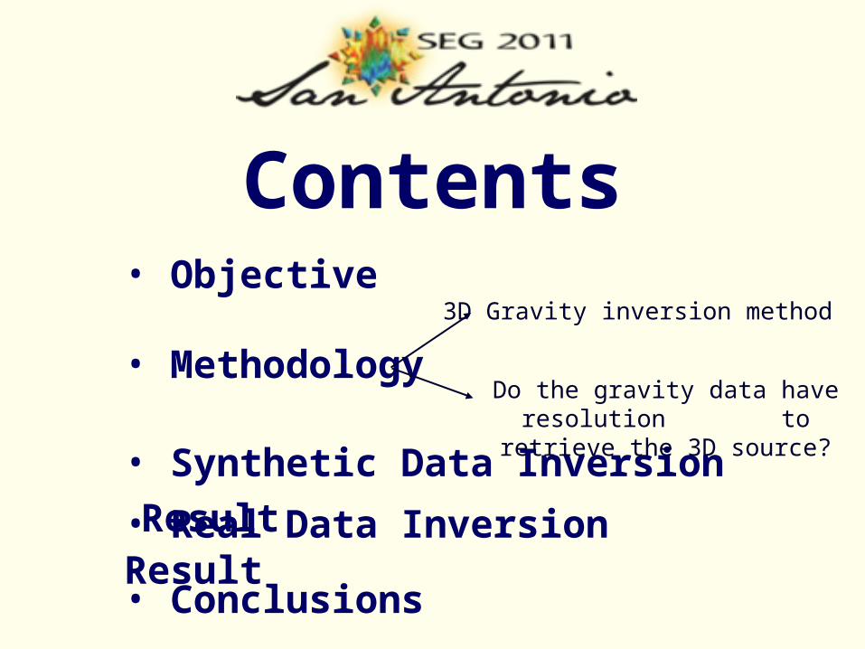
Contents• Objective
• Methodology
• Real Data Inversion Result
• Conclusions
• Synthetic Data Inversion Result
3D Gravity inversion method
Do the gravity data have resolution to retrieve the 3D source?
yxN E
zDep
thD
epth
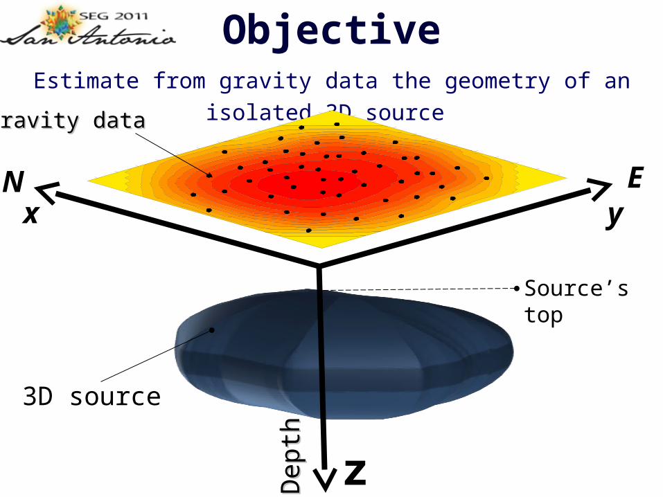
3D source
ObjectiveEstimate from gravity data the geometry of an isolated 3D source
Gravity dataGravity data
Source’s top

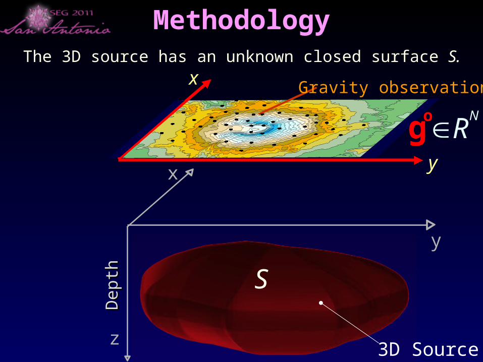
Methodology
y
x
z
y
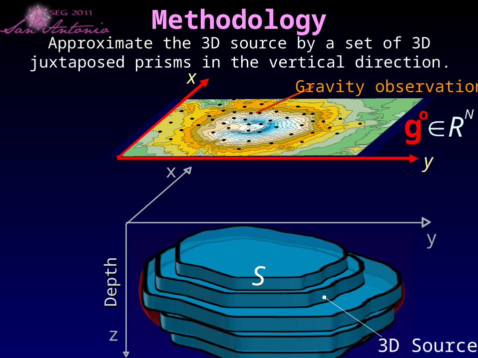
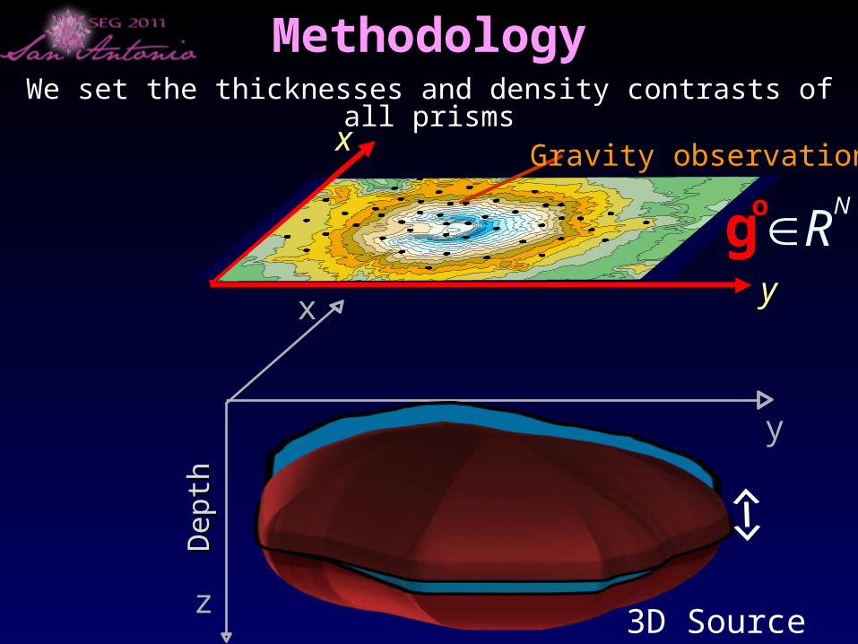
x Gravity observations
go NR
3D Source
Dep
thD
epth S
The 3D source has an unknown closed surface S.
Methodology
x
z
y
x Gravity observations
go NR
3D Source
Dep
thD
epth
Approximate the 3D source by a set of 3D juxtaposed prisms in the vertical direction .
S
y
Methodology
x
z
y
x Gravity observations
go NR
3D Source
Dep
thD
epth
We set the thicknesses and density contrasts of all prisms
y
Methodology
x
z
y
x Gravity observations
go NR
3D Source
Dep
thD
epth
y
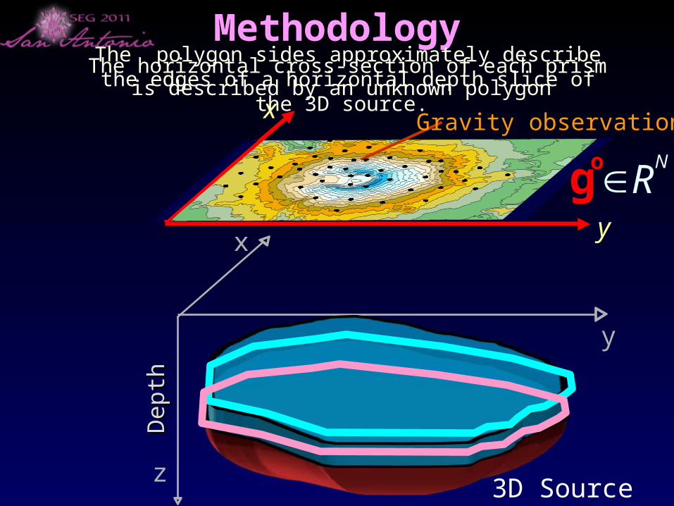
MethodologyThe horizontal cross-section of each prism is described by
an unknown polygon The polygon sides approximately describe the edges of a
horizontal depth slice of the 3D source.
y
x Gravity observations
go NR
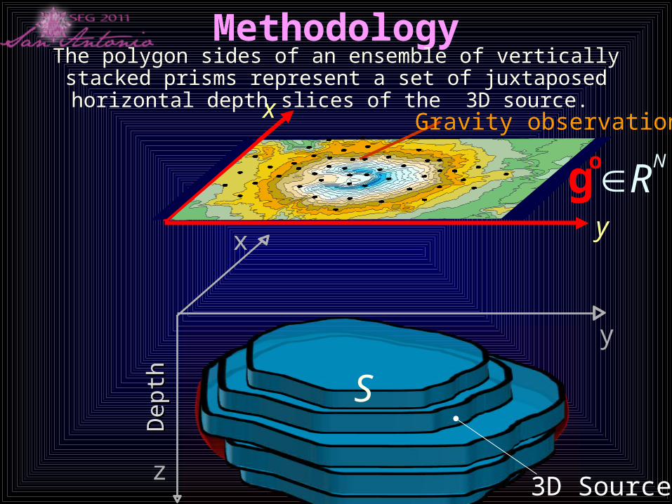
MethodologyThe polygon sides of an ensemble of vertically stacked prisms represent
a set of juxtaposed horizontal depth slices of the 3D source.
x
z3D Source
Dep
thD
epth S
y
y
x Gravity observations
go NR
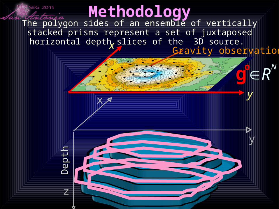
MethodologyThe polygon sides of an ensemble of vertically stacked prisms represent
a set of juxtaposed horizontal depth slices of the 3D source.
x
z
Dep
thD
epth
y
x
z
Dep
thD
epth
y
Methodology
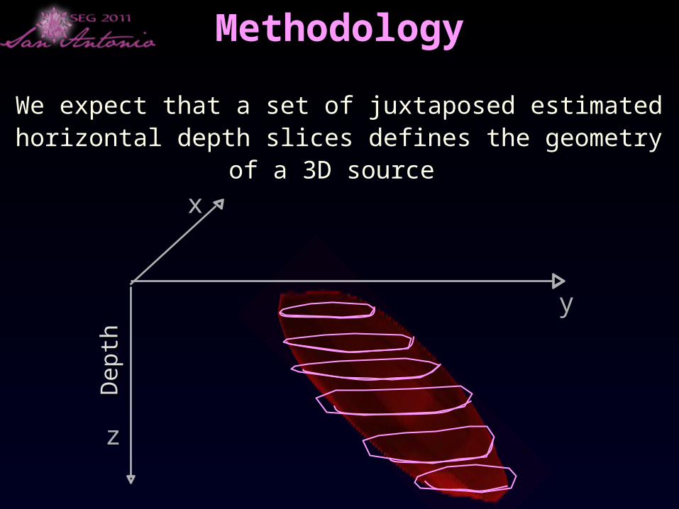
We expect that a set of juxtaposed estimated horizontal depth slices defines the geometry of a 3D source
x
z
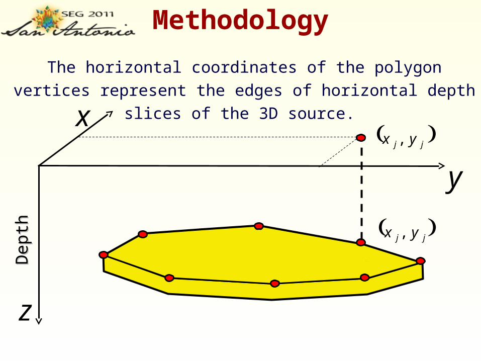
The horizontal coordinates of the polygon vertices represent the
edges of horizontal depth slices of the 3D source.
MethodologyD
epth
Dep
th
y
jj yx ,
jj yx ,
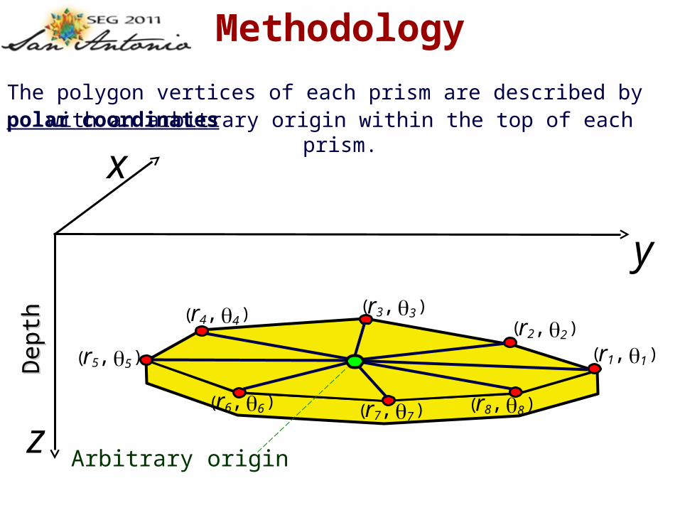
The polygon vertices of each prism are described by polar coordinates
Methodology
x
z
Dep
thD
epth
y
with an arbitrary origin within the top of each prism.
Arbitrary origin
11 r ,( )22 r ,( )
33 r ,( )( 44 r , )
( 55 r , )
( 66 r , ) ( 77 r , ) ( 88 r , )
x
z
De
pth
De
pth
y
11 r ,( )22 r ,( )
33 r ,( )( 44 r , )
( 55 r , )
( 66 r , )( 77 r , ) ( 88 r , )
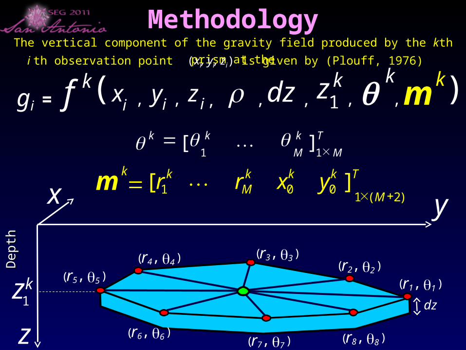
The vertical component of the gravity field produced by the kth prism at the
Methodology
),,,,,(k1kzdz
km,, iziy
ixf
k
1kz
i th observation point (xi, yi, zi) is given by (Plouff, 1976)
dz
T
M
k
M
kk
11][
TkkkM
kkyxrrm 001 ][
M )2(1
ig =
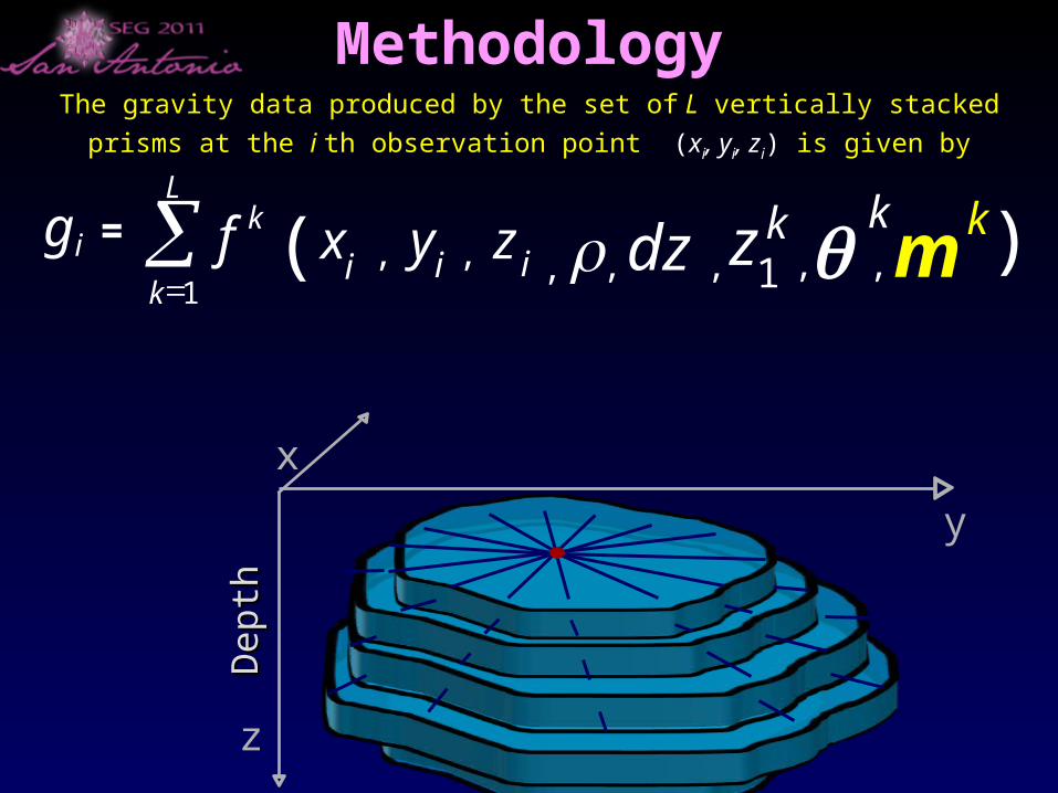
The gravity data produced by the set of L vertically stacked prisms at the i th observation
point (xi, yi, zi) is given by
Methodology
L
k
kf1
ig = ),,,,,( 1kzdz
km,, iziy
ix
k
x
z
Dep
thD
epth
y
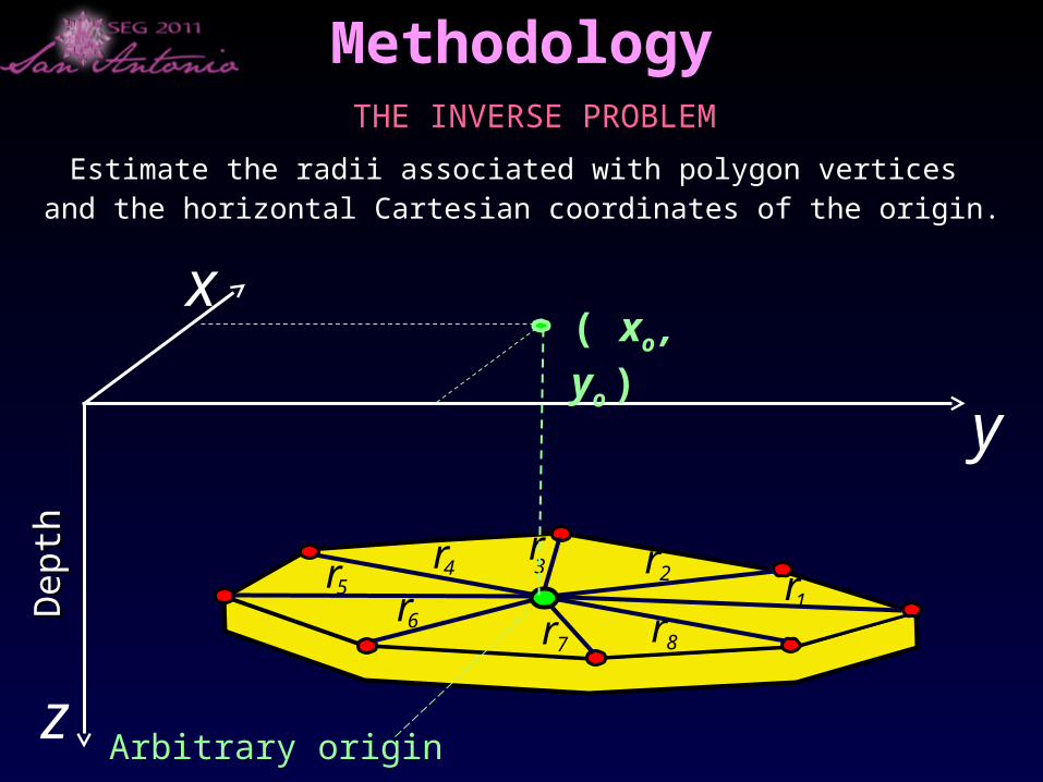
MethodologyTHE INVERSE PROBLEM
Estimate the radii associated with polygon vertices
x
z
Dep
thD
epth
y
Arbitrary origin
1r2r3
r4r
5r6r
7r 8r
and the horizontal Cartesian coordinates of the origin.
( xo , yo )
y
x Gravity observations
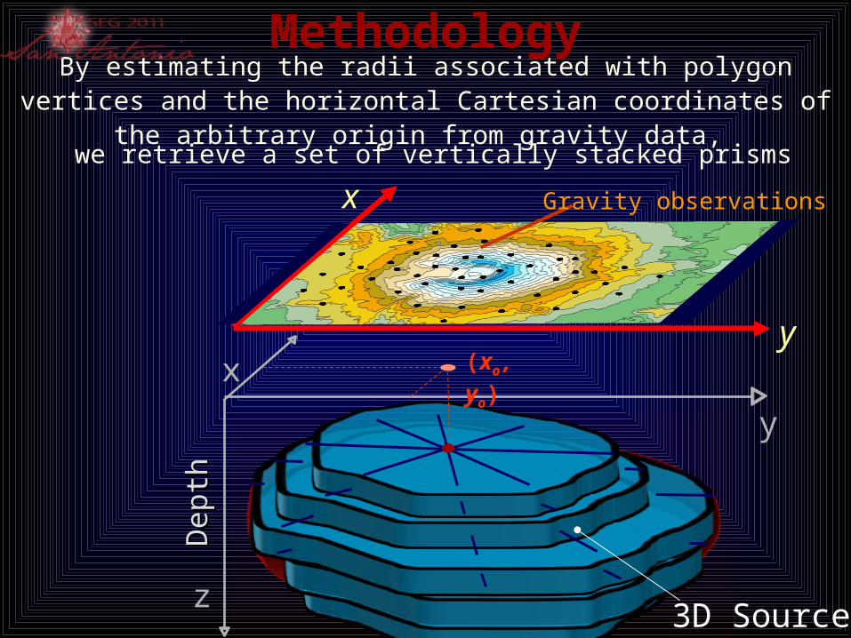
MethodologyBy estimating the radii associated with polygon vertices and the
horizontal Cartesian coordinates of the arbitrary origin from gravity data,
x
z3D Source
Dep
thD
epth
y
(xo , yo)
we retrieve a set of vertically stacked prisms
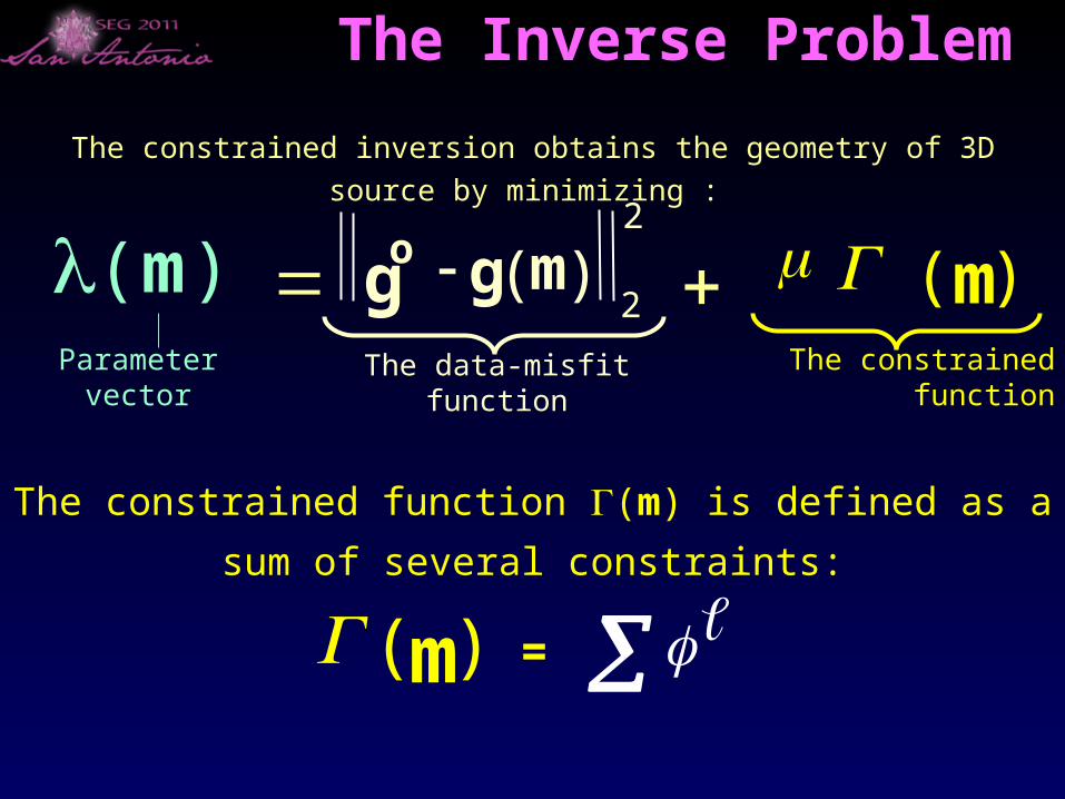
The Inverse Problem
)(mParameter vector The data-misfit function
The constrained inversion obtains the geometry of 3D source by minimizing :
)(m
2
)( mggo
2
The constrained function
)(m
=
The constrained function (m) is defined as a sum of several
constraints:
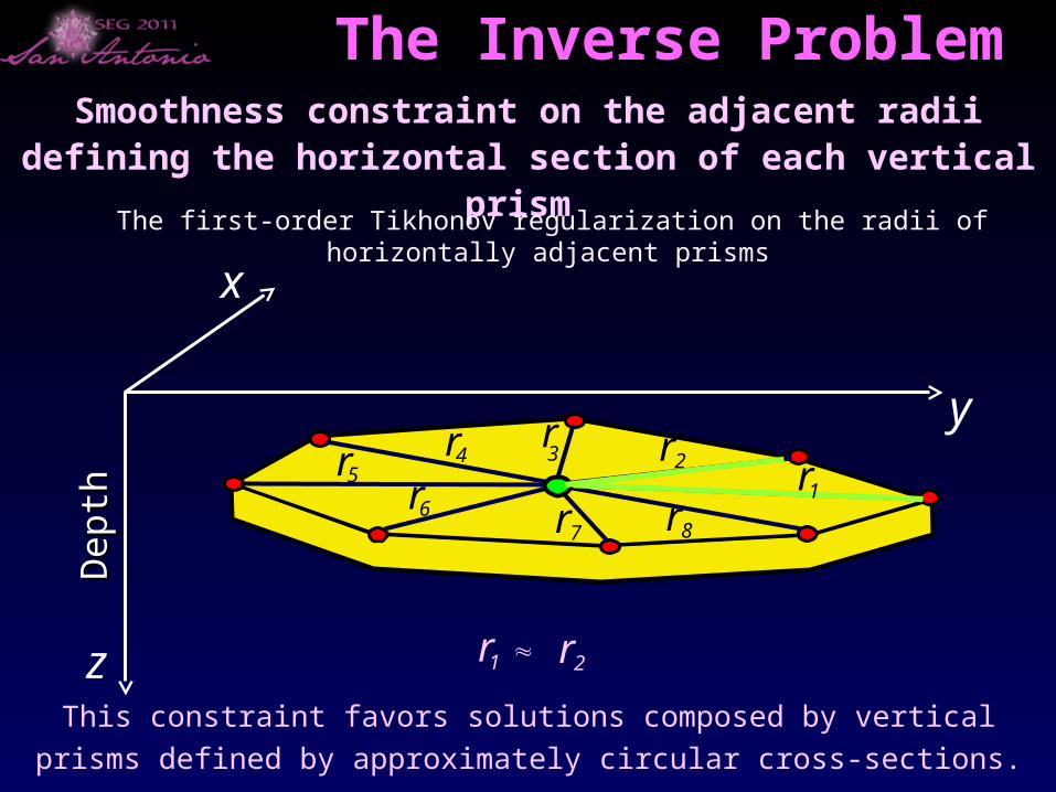
Smoothness constraint on the adjacent radii defining the horizontal section of each vertical prism
The Inverse Problem
The first-order Tikhonov regularization on the radii of horizontally adjacent prisms
x
z
Dep
thD
epth
y2r3
r4r
5r6r
7r 8r1r
This constraint favors solutions composed by vertical prisms defined by
approximately circular cross-sections.
1r 2r
kjr
1kjr
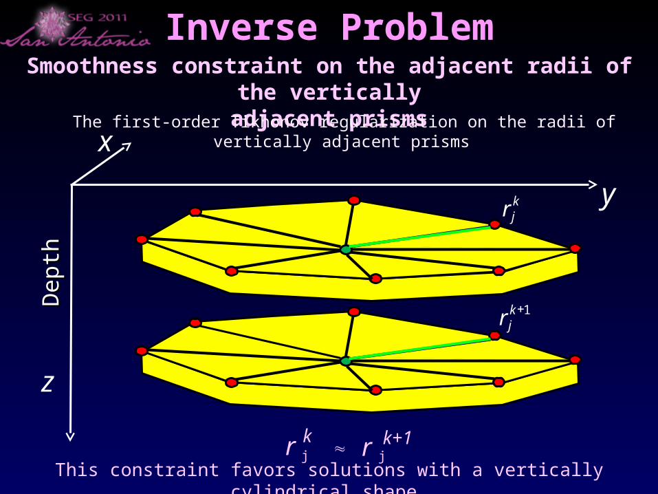
Inverse ProblemSmoothness constraint on the adjacent radii of the
verticallyadjacent prisms
x
z
Dep
thD
epth
y
The first-order Tikhonov regularization on the radii of vertically adjacent prisms
This constraint favors solutions with a vertically cylindrical shape.
jr jrk k+1
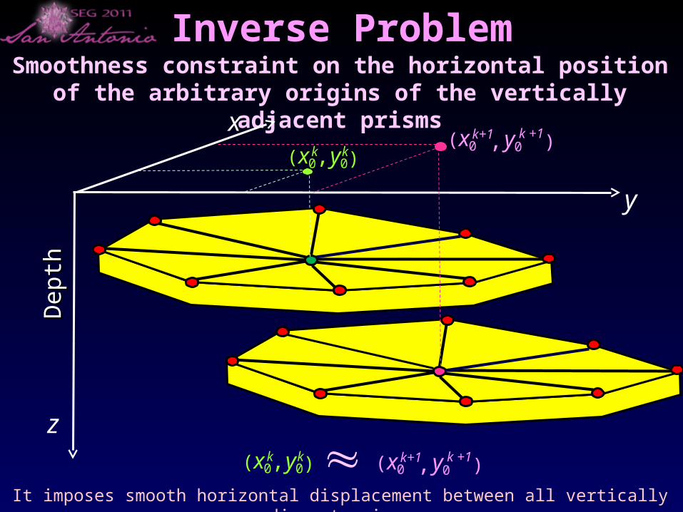
Inverse ProblemSmoothness constraint on the horizontal position of the arbitrary origins of the vertically adjacent
prisms
It imposes smooth horizontal displacement between all vertically adjacent prisms.
x
z
Dep
thD
epth
y
),( 00kk yx
),( 00k +1k+1 yx
),( 00kk yx ),( 00
k +1k+1 yx
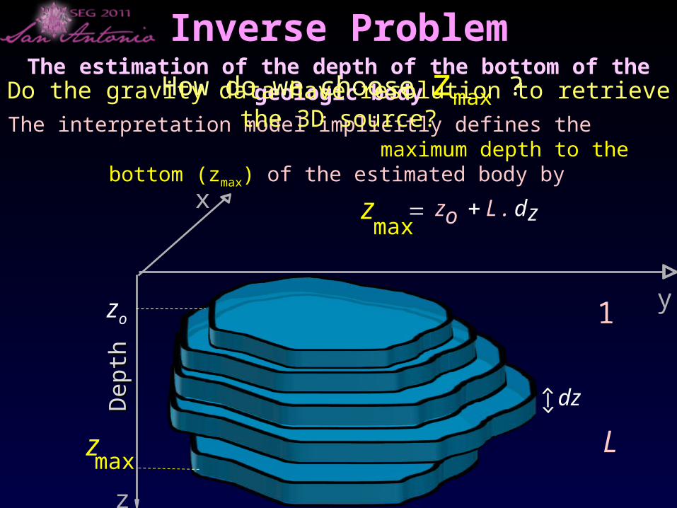
Inverse ProblemThe estimation of the depth of the bottom of the
geologic body
x
z
Dep
thD
epth
y
dz
zo
The interpretation model implicitly defines the maximum depth to the bottom (zmax) of the estimated body by
1
.
.
L
L . dzz max o z
zmax
How do we choose zmax ?Do the gravity data have resolution to retrieve the 3D source?
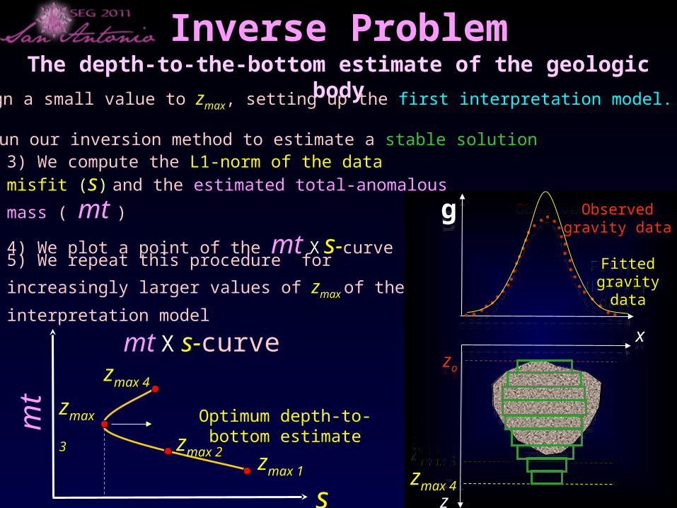
Inverse ProblemThe depth-to-the-bottom estimate of the geologic
body1) We assign a small value to zmax, setting up the first interpretation model.
gObserved gravity data
zo
zmax 1
z
x
2) We run our inversion method to estimate a stable solution
Fitted gravity data
s
mt
zmax 1
mt X s-curve
5) We repeat this procedure for increasingly larger
values of zmax of the interpretation model
zmax 2
g Observed gravity data
zo
zmax 2
z
x
Fitted gravity data
g Observed gravity data
zo
zmax 3
z
x
Fitted gravity data
zmax 3
g Observed gravity data
zo
zmax 4z
x
Fitted gravity data
4) We plot a point of the mt X s-curve
3) We compute the L1-norm of the data misfit (s) and the
estimated total-anomalous mass ( mt )
zmax 4
Optimum depth-to-bottom estimate
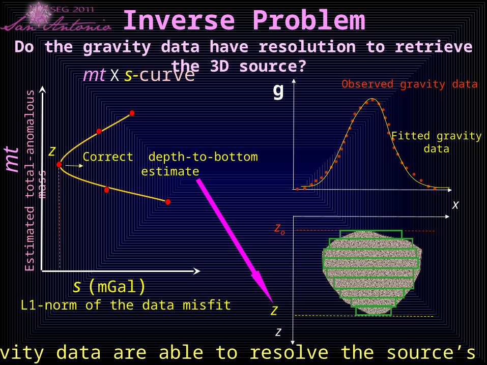
Inverse ProblemDo the gravity data have resolution to retrieve the
3D source?
Correct depth-to-bottom estimate
mt X s-curve
L1-norm of the data misfit
Est
imat
ed t
otal
-ano
mal
ous
mas
s
s (mGal)
mt
g Observed gravity data
zo
zz
x
Fitted gravity data
The gravity data are able to resolve the source’s bottom.
z
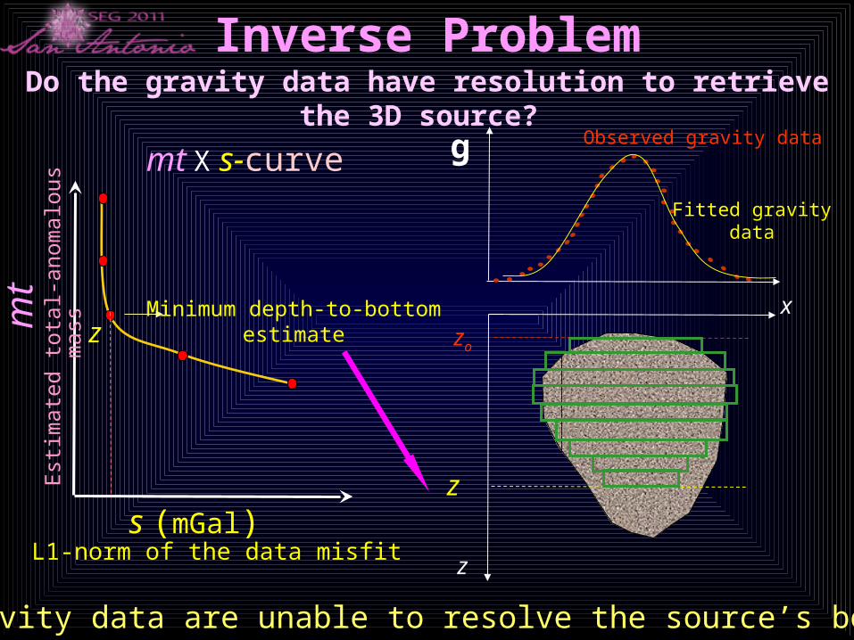
Inverse ProblemDo the gravity data have resolution to retrieve the
3D source?
Minimum depth-to-bottom estimate
s (mGal)
mt
mt X s-curve
L1-norm of the data misfit
Est
imat
ed t
otal
-ano
mal
ous
mas
s
g Observed gravity data
zo
z
z
x
Fitted gravity data
The gravity data are unable to resolve the source’s bottom.
z
INVERSION OF
SYNTHETIC GRAVITY DATA
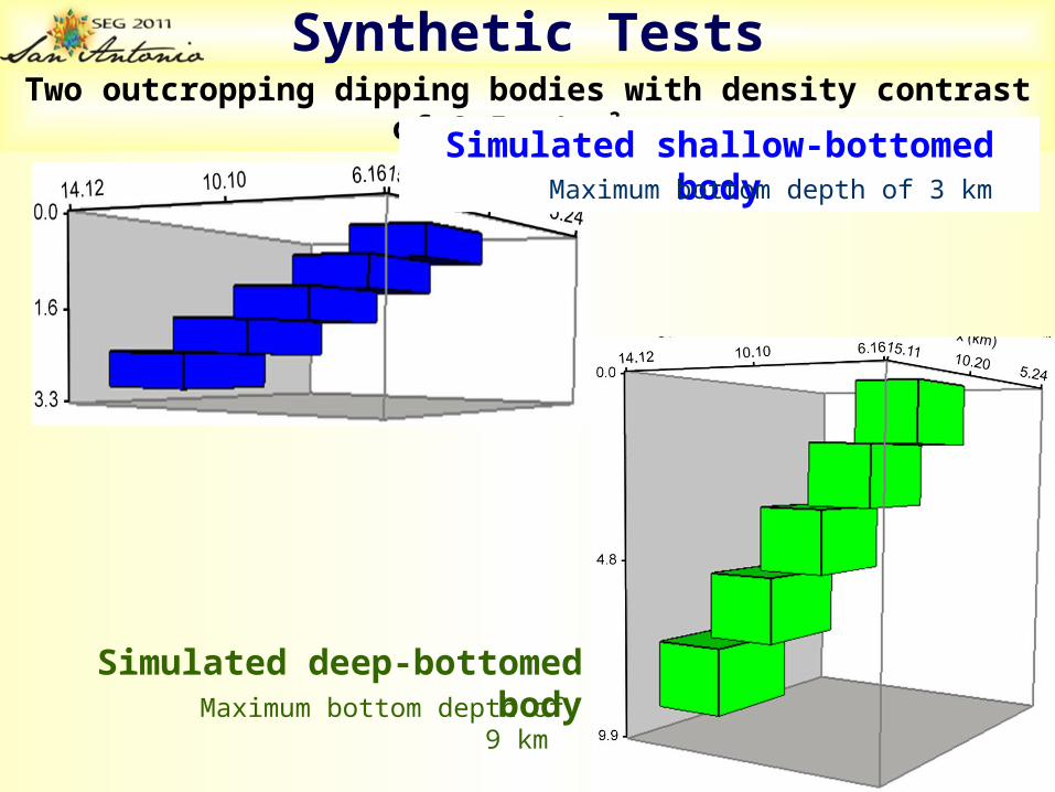
Synthetic TestsTwo outcropping dipping bodies with density contrast of 0.5 g/cm³.
Simulated shallow-bottomed body
Simulated deep-bottomed body
Maximum bottom depth of 3 km
Maximum bottom depth of 9 km
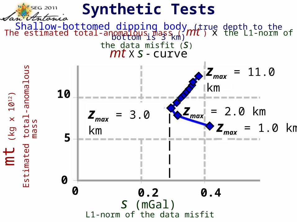
Synthetic TestsShallow-bottomed dipping body (true depth to the bottom is 3 km)
The estimated total-anomalous mass ( mt ) x the L1-norm of the data misfit (s)
s (mGal) L1-norm of the data misfit
mt (
kg x
10
12 )
Est
ima
ted
tota
l-an
om
alo
us
ma
ss
mt X s - curve
0 0.2 0.40
5
10
zmax = 1.0 km
zmax = 11.0 km
zmax = 2.0 km zmax = 3.0 km
s (mGal) L1-norm of the data misfit m
t (kg
x 1
012)
Est
ima
ted
tot
al-a
nom
alou
s m
ass
0 0.2 0.4
zmax = 1.0 km
zmax = 11.0 km
zmax = 2.0 km zmax = 3.0 km
0
5
10
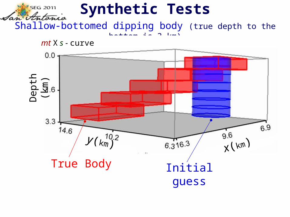
Synthetic TestsShallow-bottomed dipping body (true depth to the bottom is 3 km)
Dep
th (
km)
y(km) x(km)
Initial guessTrue Body
mt X s - curve
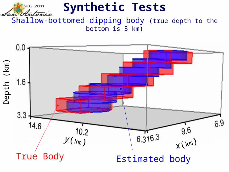
Synthetic TestsShallow-bottomed dipping body (true depth to the bottom is 3 km)
True Body Estimated body
Dep
th (
km)
x(km)y(km)
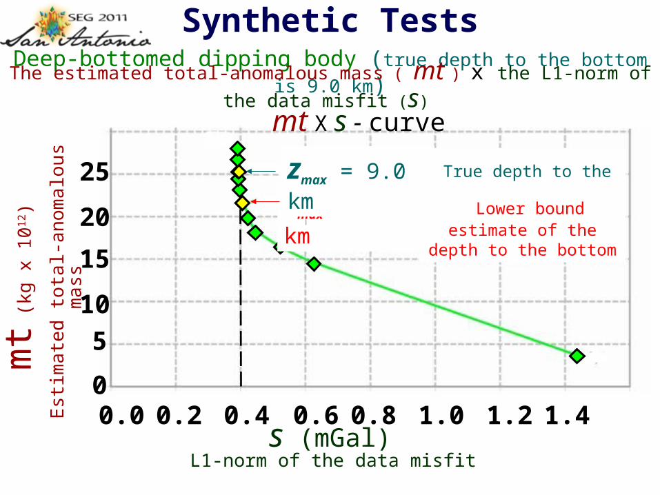
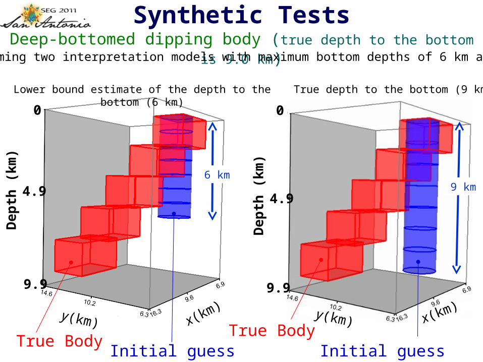
Synthetic TestsDeep-bottomed dipping body (true depth to the bottom is 9.0 km)
The estimated total-anomalous mass ( mt ) x the L1-norm of the data misfit (s)
s (mGal) L1-norm of the data misfit
mt (
kg x
10
12 )
Est
ima
ted
tota
l-an
om
alo
us
ma
ss
0.0 0.2 0.4 0.6 0.8 1.0 1.2 1.40
5
10
15
20
25zmax = 6.0 km
mt X s - curve
True depth to the bottom
Lower bound estimate of the depth to the bottom
zmax = 9.0 km
De
pth
(k
m)
x(km)y(km)
True Body
Synthetic TestsDeep-bottomed dipping body (true depth to the bottom is 9.0 km)
0
4.9
9.9
y(km) x(km)
0
4.9
9.9
By assuming two interpretation models with maximum bottom depths of 6 km and 9 km
Initial guess (6 km) Initial guess (9 km)True Body
De
pth
(k
m)
Lower bound estimate of the depth to the bottom (6 km) True depth to the bottom (9 km)
6 km9 km
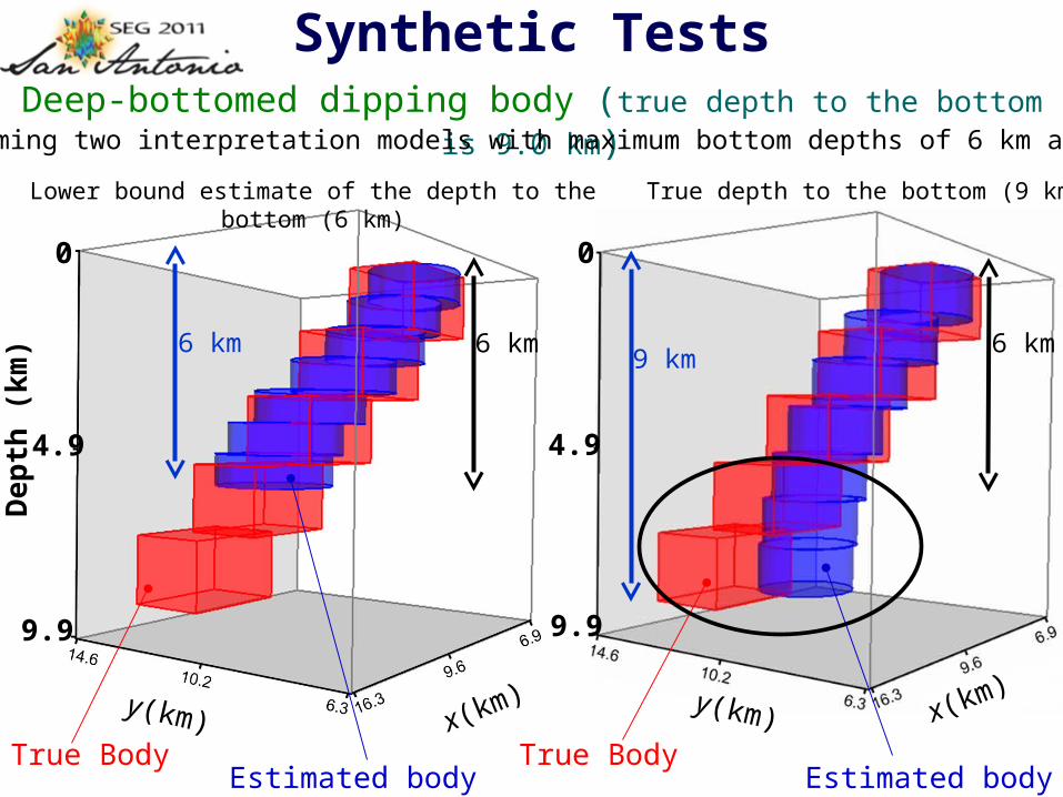
Synthetic TestsDeep-bottomed dipping body (true depth to the bottom is 9.0 km)
By assuming two interpretation models with maximum bottom depths of 6 km and 9 km
0
4.9
9.9
De
pth
(k
m)
y(km) x(km)
True Body
x(km)y(km)
0
4.9
9.9
True BodyEstimated bodyEstimated body
6 km6 km
Lower bound estimate of the depth to the bottom (6 km) True depth to the bottom (9 km)
9 km6 km
INVERSION OF
REAL GRAVITY DATA
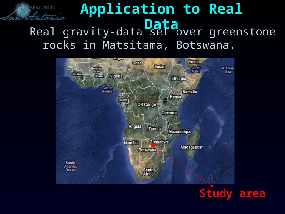
Application to Real Data
Real gravity-data set over greenstone rocks in Matsitama, Botswana.
Study area
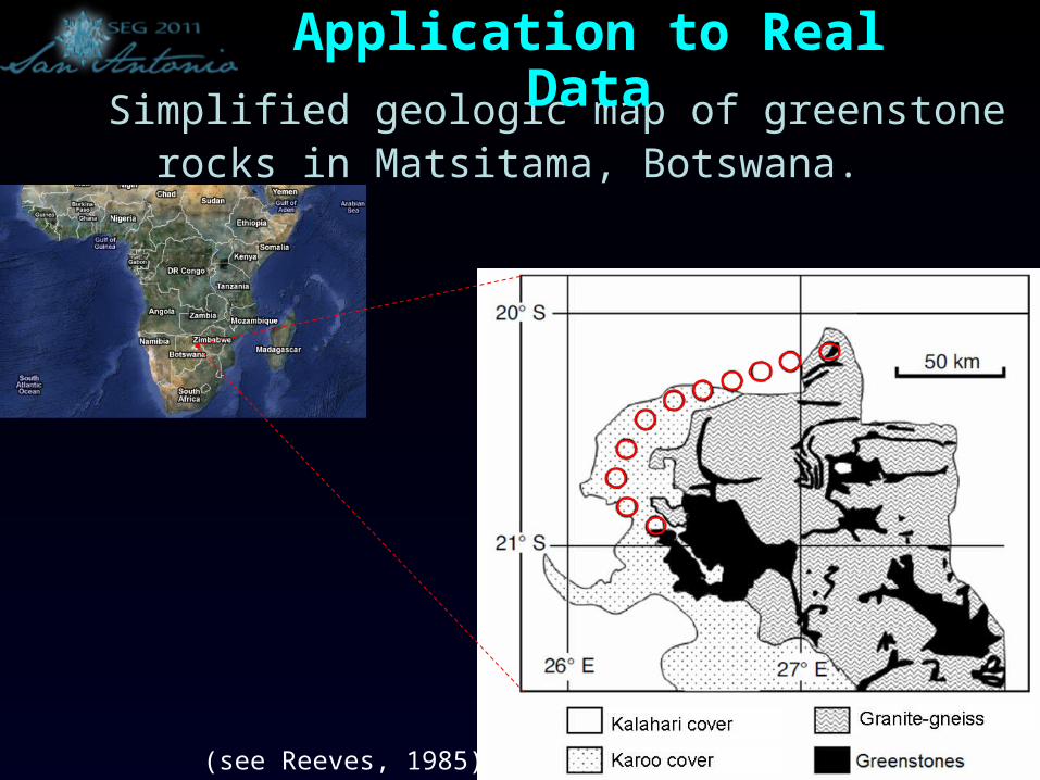
Simplified geologic map of greenstone rocks in Matsitama, Botswana.
(see Reeves, 1985)
Application to Real Data
20
20 40 60
40
60
80 100 120
80
100
120
140
160N
orth
ing
(km
)
Easting (km)
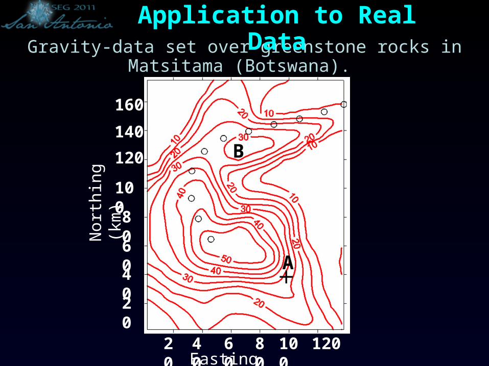
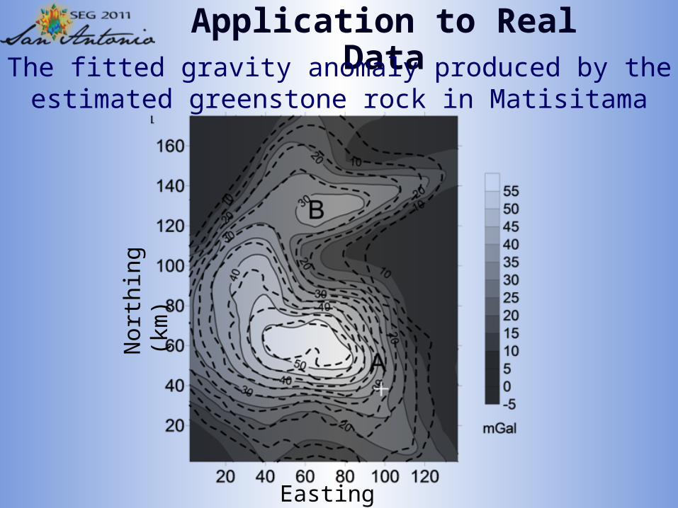
Gravity-data set over greenstone rocks in Matsitama (Botswana).
Application to Real Data
A
B
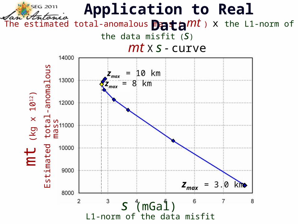
The estimated total-anomalous mass ( mt ) x the L1-norm of the data misfit (s)
Application to Real Data
s (mGal) L1-norm of the data misfit
mt (
kg x
10
12 )
Est
ima
ted
tota
l-an
om
alo
us
ma
ss
mt X s - curve
zmax = 3.0 km
zmax = 10 km zmax = 8 km
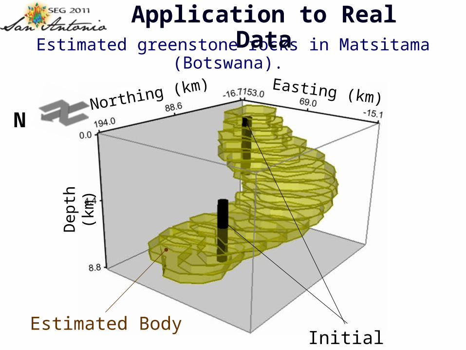
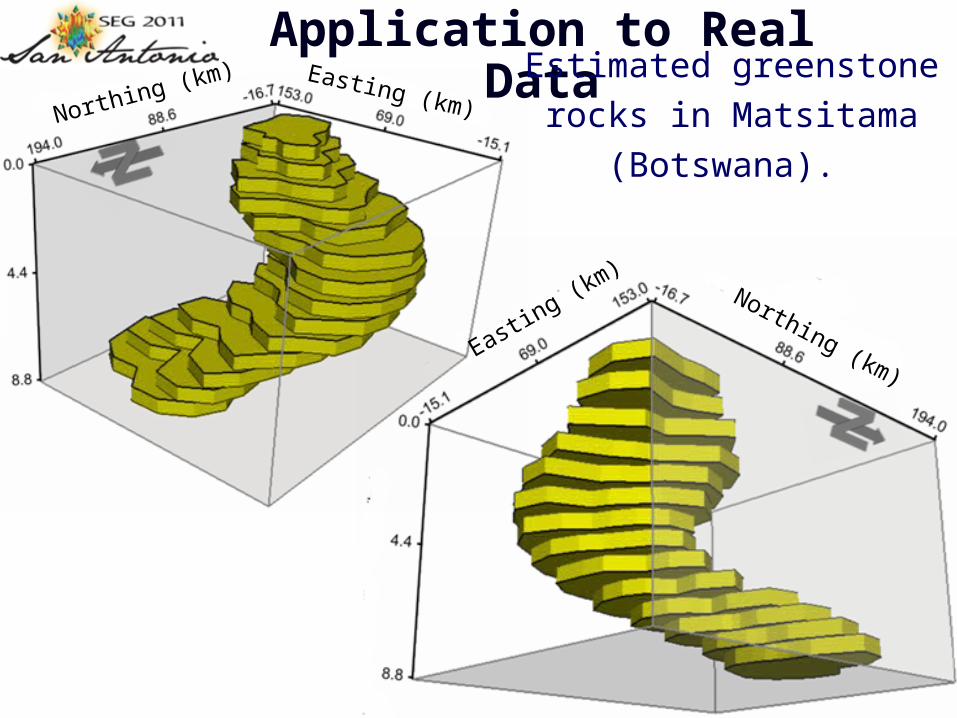
Estimated greenstone rocks in Matsitama (Botswana).
Application to Real Data
Dep
th (
km)
Estimated BodyInitial guess
Northing (km)
N
Easting (km)
Application to Real Data
Northing (km) Easting (km)
Northing (km)Easting (km)
Estimated greenstone rocks
in Matsitama (Botswana).
Application to Real Data
Nor
thin
g (k
m)
Easting (km)
The fitted gravity anomaly produced by the estimated greenstone rock in Matisitama
Conclusions
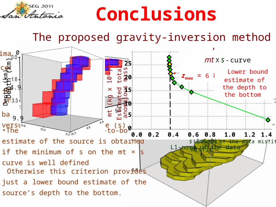
Conclusions The proposed gravity-inversion method
• Estimates the 3D geometry of isolated source
• Introduces homogeneity and compactness constraints via the interpretation model
• To reduce the class of possible solutions, we use a criterion based on the curve of
the estimated total-anomalous mass (mt) versus data-misfit measure (s).
• The solution depends on the maximum depth to
the bottom assumed for the interpretation model.
•The correct depth-to-bottom estimate of the
source is obtained if the minimum of s on the
mt × s curve is well defined
Otherwise this criterion provides just a lower
bound estimate of the source’s depth to the
bottom.
Dep
th (
km)
s (mGal) L1-norm of the data misfit
mt X s - curve
mt (
kg x
1012
)
Est
ima
ted
to
tal-a
no
ma
lou
s m
ass
0
zmax = 3.0 km
0
5
10
0.2 0.4
0
4.9
9.9
Dep
th (
km)
mt (
kg x
1012
)
Est
imat
ed to
tal-a
nom
alou
s m
ass
0.0 0.2 0.4 0.6 0.8 1.0 1.2 1.40
5
10
15
20
25
s (mGal) L1-norm of the data misfit
zmax = 6 km Lower bound estimate of the
depth to the bottom
mt X s - curve

Thank you
for your attention