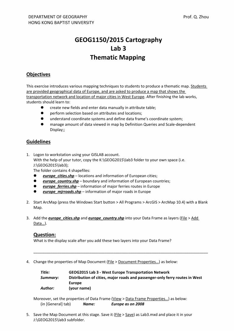
DEPARTMENT OF GEOGRAPHY  Prof. Q. Zhou HONG KONG BAPTIST UNIVERSITY 

  

GEOG1150/2015 Cartography Lab 3 

Thematic Mapping  

 Objectives  

This exercise introduces various mapping techniques to students to produce a thematic map. Students are provided geographical data of Europe, and are asked to produce a map that shows the transportation network and location of major cities in West Europe. After finishing the lab works, students should learn to: 

create new fields and enter data manually in attribute table; 

perform selection based on attributes and locations; 

understand coordinate systems and define data frame’s coordinate system; 

manage amount of data viewed in map by Definition Queries and Scale‐dependent Display;; 

 

Guidelines 

 1. Logon to workstation using your GISLAB account. 

With the help of your tutor, copy the K:\GEOG2015\lab3 folder to your own space (i.e. J:\GEOG2015\lab3); The folder contains 4 shapefiles:  europe_cities.shp – locations and information of European cities;  europe_country.shp – boundary and information of European countries;  europe_ferries.shp – information of major ferries routes in Europe  europe_mjrroads.shp – information of major roads in Europe  

2. Start ArcMap (press the Windows Start button > All Programs > ArcGIS > ArcMap 10.4) with a Blank Map.  

 3. Add the europe_cities.shp and europe_country.shp into your Data Frame as layers (File > Add 

Data…).  

Question: What is the display scale after you add these two layers into your Data Frame?   _________________________________________________________________________________ 

 4. Change the properties of Map Document (File > Document Properties…) as below: 

 Title:     GEOG2015 Lab 3 ‐ West Europe Transportation Network Summary:  Distribution of cities, major roads and passenger‐only ferry routes in West 

Europe Author:   (your name) 

 Moreover, set the properties of Data Frame (View > Data Frame Properties…) as below: 

(in [General] tab)  Name:    Europe as on 2008  5. Save the Map Document at this stage. Save it (File > Save) as Lab3.mxd and place it in your 

J:\GEOG2015\lab3 subfolder. 

6. Open the attribute table of europe_country layer (right‐click > Open Attribute Table). You may find the name (CNTRYNAME) and a field named LONG_NAME in the attribute table. 

 

Question:  What is the data types of these two fields? (hint: right‐click the field name > Properties…)  ____________________      

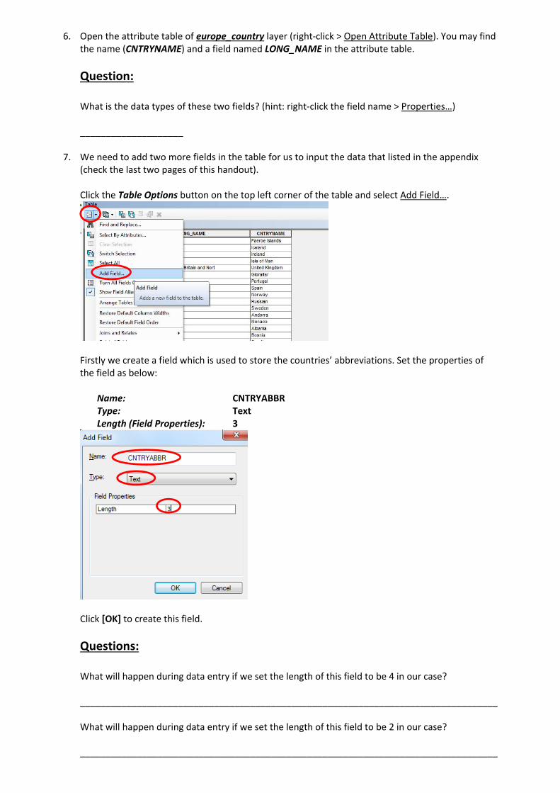
7. We need to add two more fields in the table for us to input the data that listed in the appendix (check the last two pages of this handout).  Click the Table Options button on the top left corner of the table and select Add Field….  

  Firstly we create a field which is used to store the countries’ abbreviations. Set the properties of the field as below:  

Name:         CNTRYABBR Type:        Text Length (Field Properties):  3 

  Click [OK] to create this field.  

Questions:  What will happen during data entry if we set the length of this field to be 4 in our case?  _________________________________________________________________________________  What will happen during data entry if we set the length of this field to be 2 in our case?  _________________________________________________________________________________  

 You cannot amend the field’s name, type or length once you create it. In case you set 

something incorrectly, the only thing you can do is to delete the field and recreate it 

again. 

 8. Secondly we will create another field that is used to store the countries’ area in square km. Repeat 

step 7 and set the properties of the field as below: Name:       SQKM Type:      Float Precision (Field Properties): 9 Scale (Field Properties):  2  Click [OK] to create this field. 

 

Questions:  Base on your knowledge, try to identify the most suitable field data type for the following data (circle your answer below). 

Data Input  Field Data Type 

Population in Asia countries  Short Integer / Long Integer / Float / Double / Text 

GDP per capita in Asia countries  Short Integer / Long Integer / Float / Double / Text 

Average GPA of a student  Short Integer / Long Integer / Float / Double / Text 

Number of students in a class  Short Integer / Long Integer / Float / Double / Text 

Telephone Number   Short Integer / Long Integer / Float / Double / Text 

 

 Search ArcGIS field data types in ArcGIS Desktop Help for more information  

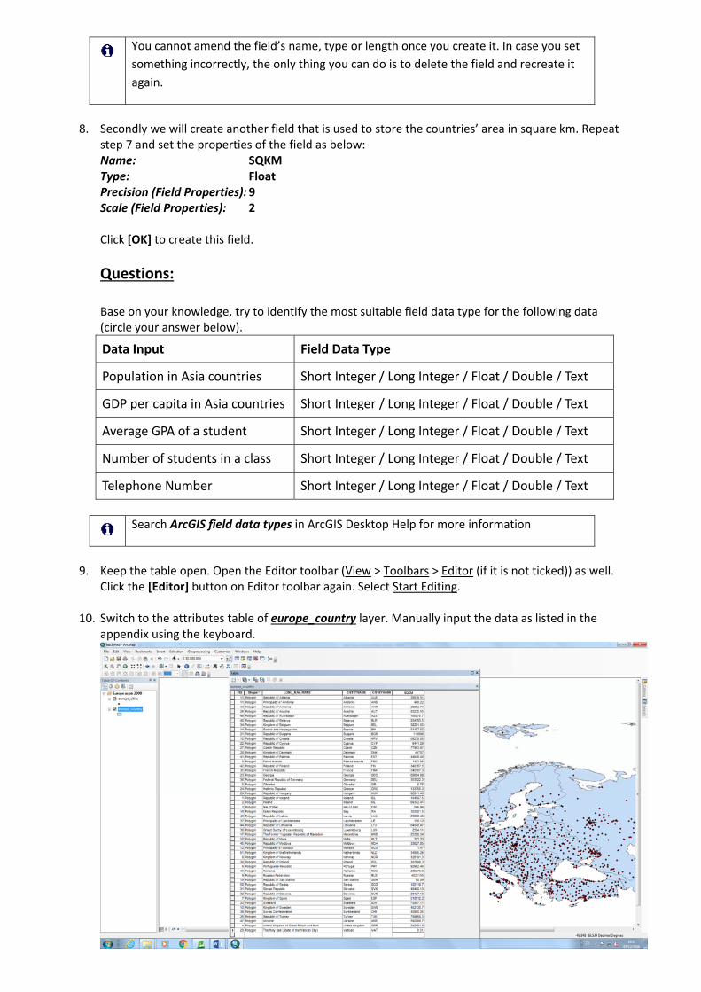
 9. Keep the table open. Open the Editor toolbar (View > Toolbars > Editor (if it is not ticked)) as well. 

Click the [Editor] button on Editor toolbar again. Select Start Editing.   

10. Switch to the attributes table of europe_country layer. Manually input the data as listed in the appendix using the keyboard.  

  

 You should sort the data in attribute table (right‐click a field > Sort Ascending or Sort 

Descending to make the data entry process easier.  

 Once you finish inputting the data (or you decide to stop for a while and resume later), switch to Editor toolbar, click the [Editor] button, select Save Edits to save your works. Then click the [Editor] button again and select Stop Editing to terminate your session.  

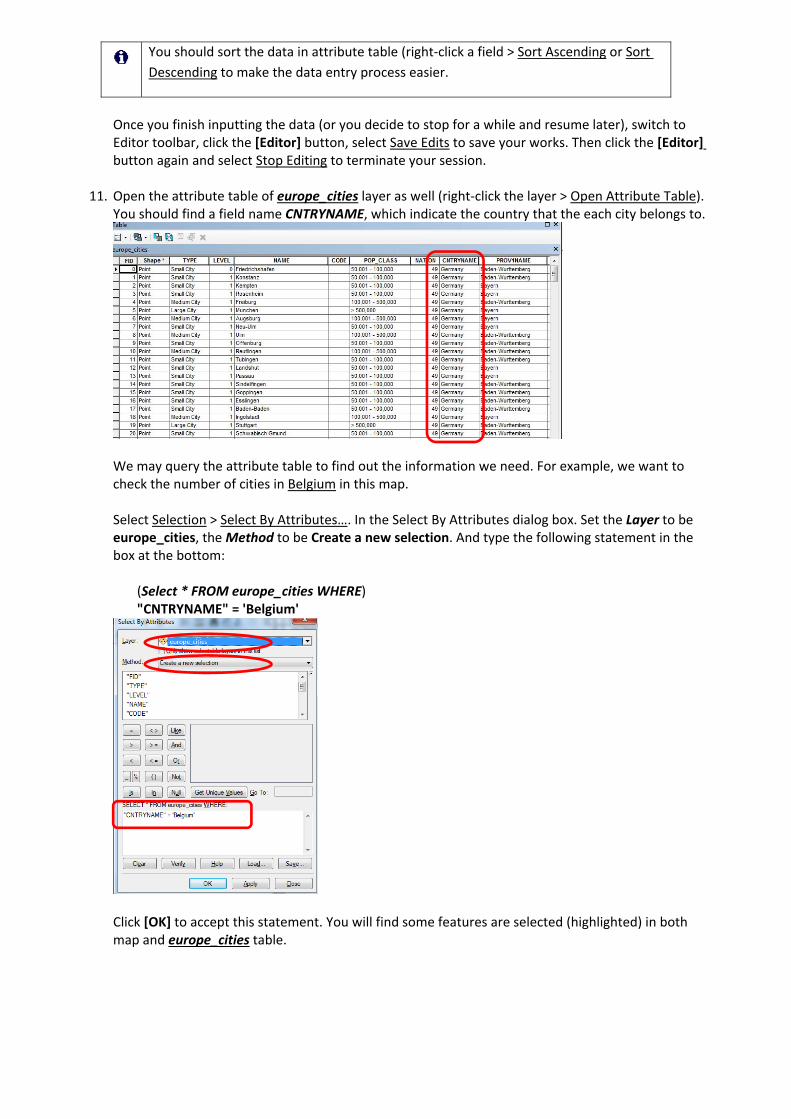
11. Open the attribute table of europe_cities layer as well (right‐click the layer > Open Attribute Table). You should find a field name CNTRYNAME, which indicate the country that the each city belongs to. 

  We may query the attribute table to find out the information we need. For example, we want to check the number of cities in Belgium in this map.  Select Selection > Select By Attributes…. In the Select By Attributes dialog box. Set the Layer to be europe_cities, the Method to be Create a new selection. And type the following statement in the box at the bottom:    (Select * FROM europe_cities WHERE)   "CNTRYNAME" = 'Belgium' 

  Click [OK] to accept this statement. You will find some features are selected (highlighted) in both map and europe_cities table.  

  

Question:  How many cities are selected?  _________________  Select Selection > Clear Selected Features after you counted the number of selected cities. 

 12. Alternatively, we may use another method to perform the same query. 

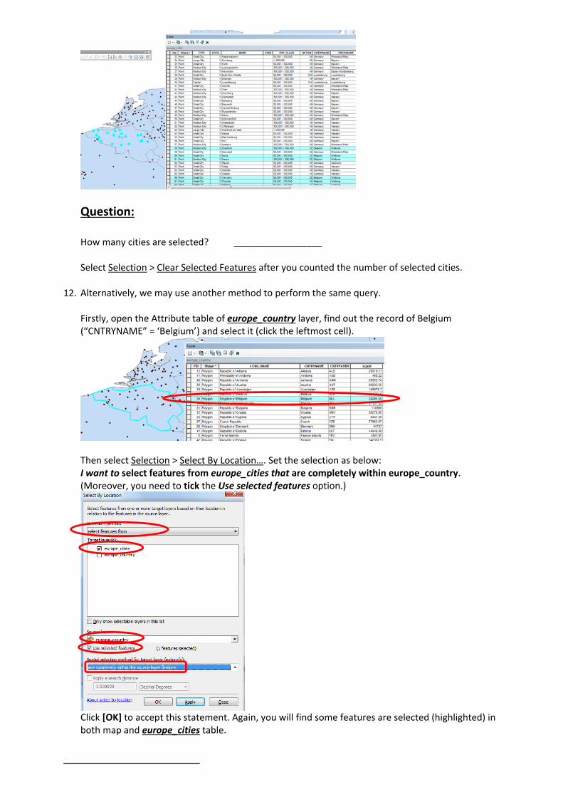
 Firstly, open the Attribute table of europe_country layer, find out the record of Belgium (“CNTRYNAME” = ‘Belgium’) and select it (click the leftmost cell). 

  Then select Selection > Select By Location…. Set the selection as below: I want to select features from europe_cities that are completely within europe_country. (Moreover, you need to tick the Use selected features option.) 

 Click [OK] to accept this statement. Again, you will find some features are selected (highlighted) in both map and europe_cities table.  

   

Question:  How many cities are selected?   _________________  Select Selection > Clear Selected Features after you counted the number of selected cities.   Moreover, you may close the europe_cities table and europe_country table.  

13. Use your own way to locate the cities Longyearbyen (in Svalbard and Jan Mayen Islands, the North most city in the map) and Telde (in Spain, the South most city in the map). 

 Use the method you learnt in step 18 of Lab 1 to measure the approximate distance between these two cities in kilometers.  

Questions:  What is the distance between Longyearbyen and Telde in this map?    ___________(km, d precision)  Why the line is not straight in this measurement?  _________________________________________________________________________________  _________________________________________________________________________________  _________________________________________________________________________________ 

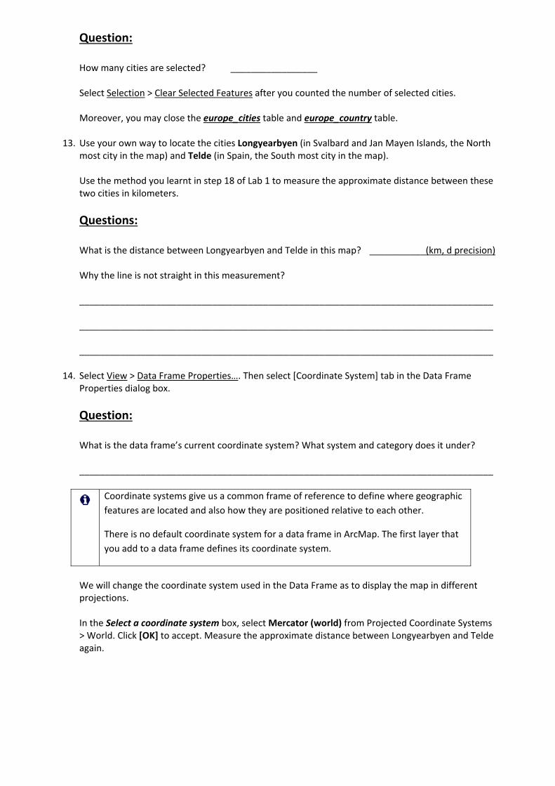
 14. Select View > Data Frame Properties…. Then select [Coordinate System] tab in the Data Frame 

Properties dialog box.  

Question:  What is the data frame’s current coordinate system? What system and category does it under?   _________________________________________________________________________________  

 Coordinate systems give us a common frame of reference to define where geographic 

features are located and also how they are positioned relative to each other.  

There is no default coordinate system for a data frame in ArcMap. The first layer that 

you add to a data frame defines its coordinate system.  

 We will change the coordinate system used in the Data Frame as to display the map in different projections.  In the Select a coordinate system box, select Mercator (world) from Projected Coordinate Systems > World. Click [OK] to accept. Measure the approximate distance between Longyearbyen and Telde again. 

   Repeat this step to change the data frame’s coordinate system to be Robinson (world) (from Projected Coordinate Systems > World), MGI_Slovenia_Grid (from Projected Coordinate Systems > National Grids > Europe) and Europe Equidistant Conic (from Projected Coordinate Systems > Continental > Europe), and measure the approximate distance between Longyearbyen and Telde.  (hint: you will get a warning message when you apply MGI Slovenia Grid and Europe Equidistant Conic coordinate system to the Data Frame. It is caused by different geographic coordinate systems between the data frame and source of layer. Click [Yes] to accept it in this case. Nevertheless a transformation may be needed to avoid misalignments caused by scale and accuracy issues in future case.)  

Question:  What are the distance between Longyearbyen and Telde (in kilometers, d precision) when you applied different coordinate systems to the Data Frame?  Mercator              ____________(km)_  Robinson              ____________(km)_  MGI Slovenia Grid              ____________(km)_  Europe Equidistant Conic              ____________(km)_ 

 

 Search What are map projections? and Coordinate systems for map display in ArcGIS 

Desktop Help for more information  

 When you finish your measurements, change the Data Frame back to its “original” coordinate system WGS 1984 (from Geographic Coordinate Systems > World). 

 15. In our map there are too many cities, which are in fact “cluttering” our map especially at smaller 

scale. We will simplify the map using definition queries and scale‐dependent display in combination.  

There are different types of cities (Capital, Large City, Medium City, Small City) in the europe_cities layer.  

   

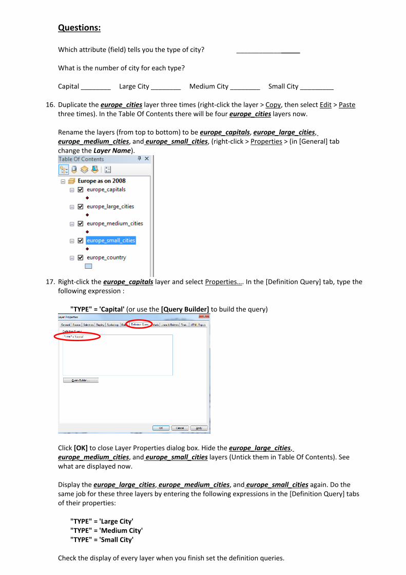
Questions:  Which attribute (field) tells you the type of city?              _________________  What is the number of city for each type?  Capital ________     Large City ________     Medium City ________     Small City _________ 

 16. Duplicate the europe_cities layer three times (right‐click the layer > Copy, then select Edit > Paste 

three times). In the Table Of Contents there will be four europe_cities layers now.   Rename the layers (from top to bottom) to be europe_capitals, europe_large_cities, europe_medium_cities, and europe_small_cities, (right‐click > Properties > (in [General] tab change the Layer Name). 

 17. Right‐click the europe_capitals layer and select Properties…. In the [Definition Query] tab, type the 

following expression :  

"TYPE" = 'Capital' (or use the [Query Builder] to build the query) 

  Click [OK] to close Layer Properties dialog box. Hide the europe_large_cities, europe_medium_cities, and europe_small_cities layers (Untick them in Table Of Contents). See what are displayed now.  Display the europe_large_cities, europe_medium_cities, and europe_small_cities again. Do the same job for these three layers by entering the following expressions in the [Definition Query] tabs of their properties:    "TYPE" = 'Large City'   "TYPE" = 'Medium City'   "TYPE" = 'Small City'  Check the display of every layer when you finish set the definition queries. 

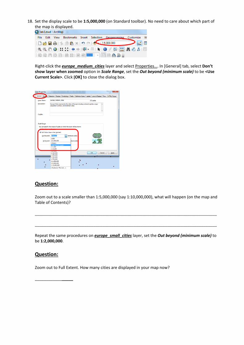
 18. Set the display scale to be 1:5,000,000 (on Standard toolbar). No need to care about which part of 

the map is displayed. 

  Right‐click the europe_medium_cities layer and select Properties…. In [General] tab, select Don’t show layer when zoomed option in Scale Range, set the Out beyond (minimum scale) to be <Use Current Scale>. Click [OK] to close the dialog box.   

   

Question:  Zoom out to a scale smaller than 1:5,000,000 (say 1:10,000,000), what will happen (on the map and Table of Contents)?  _________________________________________________________________________________  _________________________________________________________________________________  Repeat the same procedures on europe_small_cities layer, set the Out beyond (minimum scale) to be 1:2,000,000.  

 Question:  Zoom out to Full Extent. How many cities are displayed in your map now?                _________________ 

    

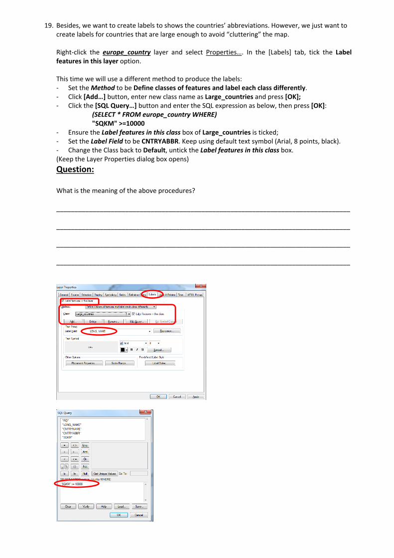
19. Besides, we want to create labels to shows the countries’ abbreviations. However, we just want to create labels for countries that are large enough to avoid “cluttering” the map. 

 Right‐click  the  europe_country  layer  and  select  Properties….  In  the  [Labels]  tab,  tick  the  Label features in this layer option.   This time we will use a different method to produce the labels: ‐ Set the Method to be Define classes of features and label each class differently.   ‐ Click [Add…] button, enter new class name as Large_countries and press [OK]; ‐ Click the [SQL Query…] button and enter the SQL expression as below, then press [OK]: 

  (SELECT * FROM europe_country WHERE)  "SQKM" >=10000 

‐ Ensure the Label features in this class box of Large_countries is ticked; ‐ Set the Label Field to be CNTRYABBR. Keep using default text symbol (Arial, 8 points, black).  ‐ Change the Class back to Default, untick the Label features in this class box. (Keep the Layer Properties dialog box opens) 

Question:  What is the meaning of the above procedures?  _________________________________________________________________________________  _________________________________________________________________________________  _________________________________________________________________________________  _________________________________________________________________________________   

  

  

   

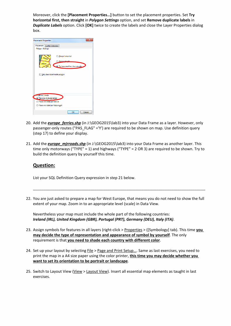
Moreover, click the [Placement Properties…] button to set the placement properties. Set Try horizontal first, then straight in Polygon Settings option, and set Remove duplicate labels in Duplicate Labels option. Click [OK] twice to create the labels and close the Layer Properties dialog box.  

  20. Add the europe_ferries.shp (in J:\GEOG2015\lab3) into your Data Frame as a layer. However, only 

passenger‐only routes ("PAS_FLAG" ='Y') are required to be shown on map. Use definition query (step 17) to define your display. 

 21. Add the europe_mjrroads.shp (in J:\GEOG2015\lab3) into your Data Frame as another layer. This 

time only motorways (“TYPE” = 1) and highways (“TYPE” = 2 OR 3) are required to be shown. Try to build the definition query by yourself this time. 

 

Question:  List your SQL Definition Query expression in step 21 below.  _________________________________________________________________________________  

22. You are just asked to prepare a map for West Europe, that means you do not need to show the full extent of your map. Zoom in to an appropriate level (scale) in Data View.   Nevertheless your map must include the whole part of the following countries:  Ireland (IRL), United Kingdom (GBR), Portugal (PRT), Germany (DEU), Italy (ITA). 

 23. Assign symbols for features in all layers (right‐click > Properties > ([Symbology] tab). This time you 

may decide the type of representation and appearance of symbol by yourself. The only requirement is that you need to shade each country with different color.  

 24. Set up your layout by selecting File > Page and Print Setup…. Same as last exercises, you need to 

print the map in a A4 size paper using the color printer, this time you may decide whether you want to set its orientation to be portrait or landscape. 

 25. Switch to Layout View (View > Layout View). Insert all essential map elements as taught in last 

exercises.  

   

Question:  Do you think a legend for europe_country layer is needed here? Why?  _________________________________________________________________________________  _________________________________________________________________________________  Preview the layout. If it is okay, print it out using the color printer. 

 

Question: 

(Print the layout out in a A4 size paper using color printer) 

26. Save the Map Document (File > Save) again. Quit ArcMap (File > Exit). Turn off your workstation 

before you leave. 

 ArcGIS Desktop Help can be reached by selecting Help > ArcGIS Desktop Help (or 

ArcGIS Desktop Web Help) in most of the ArcGIS applications.  

 

   

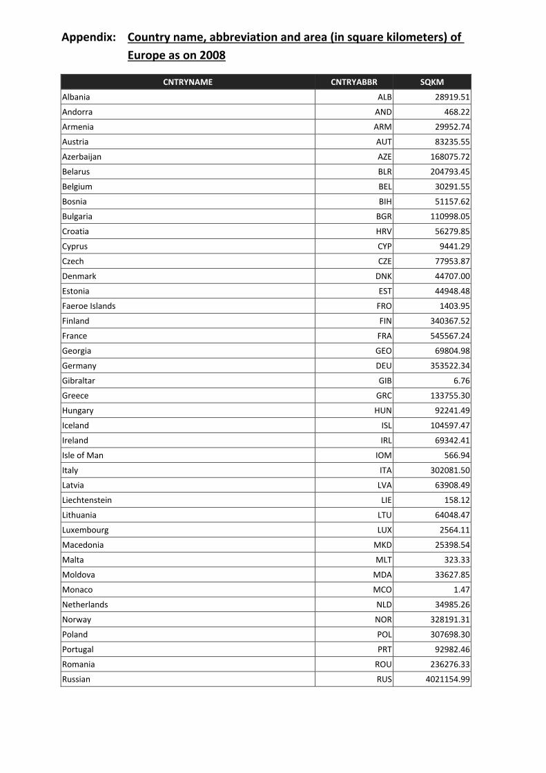
Appendix:  Country name, abbreviation and area (in square kilometers) of 

    Europe as on 2008 

CNTRYNAME  CNTRYABBR  SQKM 

Albania  ALB  28919.51

Andorra  AND  468.22

Armenia  ARM  29952.74

Austria  AUT  83235.55

Azerbaijan  AZE  168075.72

Belarus  BLR  204793.45

Belgium  BEL  30291.55

Bosnia  BIH  51157.62

Bulgaria  BGR  110998.05

Croatia  HRV  56279.85

Cyprus  CYP  9441.29

Czech  CZE  77953.87

Denmark  DNK  44707.00

Estonia  EST  44948.48

Faeroe Islands  FRO  1403.95

Finland  FIN  340367.52

France  FRA  545567.24

Georgia  GEO  69804.98

Germany  DEU  353522.34

Gibraltar  GIB  6.76

Greece  GRC  133755.30

Hungary  HUN  92241.49

Iceland  ISL  104597.47

Ireland  IRL  69342.41

Isle of Man  IOM  566.94

Italy  ITA  302081.50

Latvia  LVA  63908.49

Liechtenstein  LIE  158.12

Lithuania  LTU  64048.47

Luxembourg  LUX  2564.11

Macedonia  MKD  25398.54

Malta  MLT  323.33

Moldova  MDA  33627.85

Monaco  MCO  1.47

Netherlands  NLD  34985.26

Norway  NOR  328191.31

Poland  POL  307698.30

Portugal  PRT  92982.46

Romania  ROU  236276.33

Russian  RUS  4021154.99

   

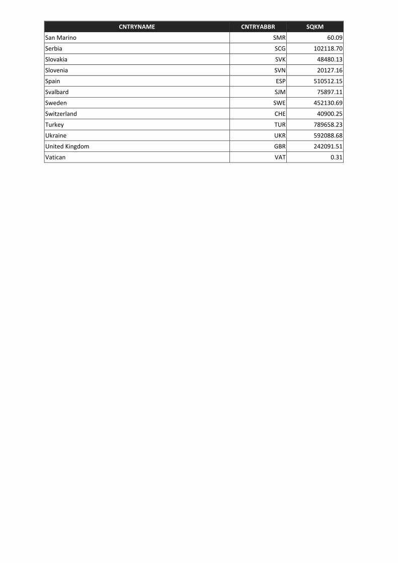
CNTRYNAME  CNTRYABBR  SQKM 

San Marino  SMR  60.09

Serbia  SCG  102118.70

Slovakia  SVK  48480.13

Slovenia  SVN  20127.16

Spain  ESP  510512.15

Svalbard  SJM  75897.11

Sweden  SWE  452130.69

Switzerland  CHE  40900.25

Turkey  TUR  789658.23

Ukraine  UKR  592088.68

United Kingdom  GBR  242091.51

Vatican  VAT  0.31