Embed Size (px)
Citation preview

Fully-Connected Tensor Network Decomposition and Its Application toHigher-Order Tensor Completion
Yu-Bang Zheng1
Ting-Zhu Huang1, Xi-Le Zhao1, Qibin Zhao2, Tai-Xiang Jiang3
1University of Electronic Science and Technology of China, China2Tensor Learning Team, RIKEN AIP, Japan
3Southwestern University of Finance and Economics, China
AAAI 2021
Yu-Bang Zheng (UESTC) FCTN Decomposition 1 / 29

Outline
1 Background and Motivation
2 FCTN Decomposition
3 FCTN-TC Model and Solving Algorithm
4 Numerical Experiments
5 Conclusion
Yu-Bang Zheng (UESTC) FCTN Decomposition 2 / 29

Background and Motivation
Outline
1 Background and Motivation
2 FCTN Decomposition
3 FCTN-TC Model and Solving Algorithm
4 Numerical Experiments
5 Conclusion
Yu-Bang Zheng (UESTC) FCTN Decomposition 3 / 29

Background and Motivation
Higher-Order Tensors
Many real-world data are higher-order tensors: e.g., color video, hyperspectral image,and traffic data.
color video hyperspectral image traffic data
Yu-Bang Zheng (UESTC) FCTN Decomposition 4 / 29

Background and Motivation
Tensor Completion
Missing Values Problems: recommender system design, image/video inpainting, andtraffic data completion.
recommender system hyperspectral image traffic data
Tensor Completion (TC): complete a tensor from its partial observation.
Yu-Bang Zheng (UESTC) FCTN Decomposition 5 / 29

Background and Motivation
Ill-Posed Inverse Problem
Ill-posed inverse problem
⇑
Prior/Intrinsic property
Piecewise smoothness
Nonlocal self-similarity
Low-rankness
⇒
Low-Rank Tensor Decomposition (Φ)
minX ,G
12‖X − Φ(G1,G2, · · · ,GN)‖2
F,
s.t. PΩ(X ) = PΩ(F).
Minimizing Tensor Rank
minX
Rank(X ),
s.t. PΩ(X ) = PΩ(F).
Here F ∈ RI1×I2×···×IN is an incomplete observation of X ∈ RI1×I2×···×IN , Ω is the indexof the known elements, and PΩ(X ) is a projection operator which projects the elementsin Ω to themselves and all others to zeros.
Yu-Bang Zheng (UESTC) FCTN Decomposition 6 / 29
Background and Motivation
Tensor Decomposition
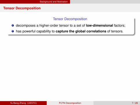
Tensor Decomposition
decomposes a higher-order tensor to a set of low-dimensional factors;
has powerful capability to capture the global correlations of tensors.
X = G ×1 U(1) ×2 U(2) ×3 · · · ×N U(N)
Tucker decomposition
X =
R∑r=1
λr g(1)r g(2)
r · · · g(N)r
CANDECOMP/PARAFAC (CP) decomposition
Yu-Bang Zheng (UESTC) FCTN Decomposition 7 / 29

Background and Motivation
Tensor Decomposition
Tensor Decomposition
decomposes a higher-order tensor to a set of low-dimensional factors;
has powerful capability to capture the global correlations of tensors.
X = G ×1 U(1) ×2 U(2) ×3 · · · ×N U(N)
Tucker decomposition
X =R∑
r=1
λr g(1)r g(2)
r · · · g(N)r
CANDECOMP/PARAFAC (CP) decomposition
Yu-Bang Zheng (UESTC) FCTN Decomposition 7 / 29

Background and Motivation
Tensor Decomposition
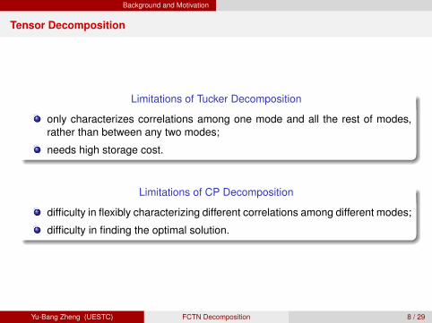
Limitations of Tucker Decomposition
only characterizes correlations among one mode and all the rest of modes,rather than between any two modes;
needs high storage cost.
Limitations of CP Decomposition
difficulty in flexibly characterizing different correlations among different modes;
difficulty in finding the optimal solution.
Yu-Bang Zheng (UESTC) FCTN Decomposition 8 / 29
Background and Motivation
Tensor Decomposition
Limitations of Tucker Decomposition
only characterizes correlations among one mode and all the rest of modes,rather than between any two modes;
needs high storage cost.
Limitations of CP Decomposition
difficulty in flexibly characterizing different correlations among different modes;
difficulty in finding the optimal solution.
Yu-Bang Zheng (UESTC) FCTN Decomposition 8 / 29

Background and Motivation
Tensor Decompositions
Recently, the popular tensor train (TT) and tensor ring (TR) decompositions haveemerged and shown great ability to deal with higher-order, especially beyond third-order tensors.
G1 G2
I1 I2
R1 R2GN
IN
RN -1X
I1
I2
I3 I4
IN
Ik
...
...
...
X (i1, i2, · · · , iN) =
R1∑r1=1
R2∑r2=1
· · ·RN−1∑
rN−1=1G1(i1, r1)G2(r1, i2, r2) · · ·GN(rN−1, iN)
TT decomposition
G1
G2
G3 G4
I1
I3 I4
I2
R1
R3
R2
GN
Gk
RN
R4
Rk
IN
Ik...Rk -1
...
RN -1
X
I1
I2
I3 I4
IN
Ik
...
...
X (i1, i2, · · · , iN) =
R1∑r1=1
R2∑r2=1
· · ·RN∑
rN=1G1(rN , i1, r1)G2(r1, i2, r2) · · · GN(rN−1, iN , rN)
TR decomposition
Yu-Bang Zheng (UESTC) FCTN Decomposition 9 / 29

Background and Motivation
Tensor Decompositions
Recently, the popular tensor train (TT) and tensor ring (TR) decompositions haveemerged and shown great ability to deal with higher-order, especially beyond third-order tensors.
G1 G2
I1 I2
R1 R2GN
IN
RN - 1X
I1
I2
I3 I4
IN
Ik
...
...
...
X (i1, i2, · · · , iN) =
R1∑r1=1
R2∑r2=1
· · ·RN−1∑
rN−1=1G1(i1, r1)G2(r1, i2, r2) · · ·GN(rN−1, iN)
TT decomposition
G1
G2
G3 G4
I1
I3 I4
I2
R1
R3
R2
GN
Gk
RN
R4
Rk
IN
Ik...Rk - 1
...
RN - 1
X
I1
I2
I3 I4
IN
Ik
...
...
X (i1, i2, · · · , iN) =
R1∑r1=1
R2∑r2=1
· · ·RN∑
rN=1G1(rN , i1, r1)G2(r1, i2, r2) · · · GN(rN−1, iN , rN)
TR decomposition
Yu-Bang Zheng (UESTC) FCTN Decomposition 9 / 29

Background and Motivation
Motivations
Limitations of TT and TR Decomposition
A limited correlation characterization: only establish a connection (opera-tion) between adjacent two factors, rather than any two factors;
Without transpositional invariance: keep the invariance only when the ten-sor modes make a reverse permuting (TT and TR) or a circular shifting (onlyTR), rather than any permuting.
Examples: reverse permuting: [1, 2, 3, 4]→ [4, 3, 2, 1]; circular shifting: [1, 2, 3, 4]→ [2, 3, 4, 1], [3, 4, 1, 2], [4, 1, 2, 3].
How to break through?
Yu-Bang Zheng (UESTC) FCTN Decomposition 10 / 29
FCTN Decomposition
Outline
1 Background and Motivation
2 FCTN Decomposition
3 FCTN-TC Model and Solving Algorithm
4 Numerical Experiments
5 Conclusion
Yu-Bang Zheng (UESTC) FCTN Decomposition 11 / 29

FCTN Decomposition
FCTN Decomposition
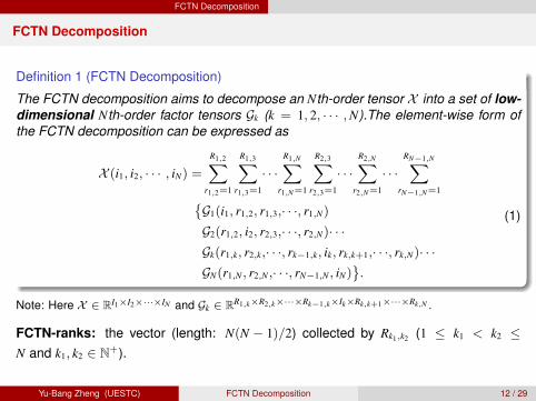
Definition 1 (FCTN Decomposition)
The FCTN decomposition aims to decompose an Nth-order tensor X into a set of low-dimensional Nth-order factor tensors Gk (k = 1, 2, · · · ,N).The element-wise form ofthe FCTN decomposition can be expressed as
X (i1, i2, · · · , iN) =
R1,2∑r1,2=1
R1,3∑r1,3=1
· · ·R1,N∑
r1,N=1
R2,3∑r2,3=1
· · ·R2,N∑
r2,N=1
· · ·RN−1,N∑
rN−1,N=1G1(i1, r1,2, r1,3,· · ·, r1,N)
G2(r1,2, i2, r2,3,· · ·, r2,N)· · ·Gk(r1,k, r2,k,· · ·, rk−1,k, ik, rk,k+1,· · ·, rk,N)· · ·GN(r1,N , r2,N ,· · ·, rN−1,N , iN)
.
(1)
Note: Here X ∈ RI1×I2×···×IN and Gk ∈ RR1,k×R2,k×···×Rk−1,k×Ik×Rk,k+1×···×Rk,N .
FCTN-ranks: the vector (length: N(N − 1)/2) collected by Rk1,k2 (1 ≤ k1 < k2 ≤N and k1, k2 ∈ N+).
Yu-Bang Zheng (UESTC) FCTN Decomposition 12 / 29
FCTN Decomposition
FCTN Decomposition
Definition 1 (FCTN Decomposition)
The FCTN decomposition aims to decompose an Nth-order tensor X into a set of low-dimensional Nth-order factor tensors Gk (k = 1, 2, · · · ,N).The element-wise form ofthe FCTN decomposition can be expressed as
X (i1, i2, · · · , iN) =
R1,2∑r1,2=1
R1,3∑r1,3=1
· · ·R1,N∑
r1,N=1
R2,3∑r2,3=1
· · ·R2,N∑
r2,N=1
· · ·RN−1,N∑
rN−1,N=1G1(i1, r1,2, r1,3,· · ·, r1,N)
G2(r1,2, i2, r2,3,· · ·, r2,N)· · ·Gk(r1,k, r2,k,· · ·, rk−1,k, ik, rk,k+1,· · ·, rk,N)· · ·GN(r1,N , r2,N ,· · ·, rN−1,N , iN)
.
(1)
Note: Here X ∈ RI1×I2×···×IN and Gk ∈ RR1,k×R2,k×···×Rk−1,k×Ik×Rk,k+1×···×Rk,N .
FCTN-ranks: the vector (length: N(N − 1)/2) collected by Rk1,k2 (1 ≤ k1 < k2 ≤N and k1, k2 ∈ N+).
Yu-Bang Zheng (UESTC) FCTN Decomposition 12 / 29

FCTN Decomposition
FCTN Decomposition
G1
G2 G3
G4
I1
I3
I4
I2
R1 ,2
R1 ,4
R2 ,4
R3 ,4
R1 ,3
R2 ,3
X
I1
I2 I3
I4
G1
G2
G3 G4
I1
I3 I4
I2
R1 ,2
R2 ,4
R3 ,4
R2 ,3
R2 ,k
GN
Gk
R1 ,k
R1 ,N
R1 ,4R1 ,3
R2 ,N
R3 ,k
R3 ,NR4 ,N
R4 ,5
Rk ,k+1
IN
IkX
I1
I2
I3 I4
IN
Ik
G1 G2
R1 ,2I1 I2X
I1 I2
G1
G2 G3
R1 ,2 R1 ,3
R2 ,3
I1
I2 I3
X
I1
I2 I3
...
...
...
...
...
...
...
... ...
...
Rk - 1 ,k
...
RN - 1 ,N
...
...
Figure 1: The Fully-Connected Tensor Network Decomposition.
Rk1,k2 : characterizes the intrinsic correlations between the k1th and k2th modes of X .
FCTN Decomposition: characterizes the correlations between any two modes.
Yu-Bang Zheng (UESTC) FCTN Decomposition 13 / 29

FCTN Decomposition
FCTN Decomposition
G1
G2 G3
G4
I1
I3
I4
I2
R1 ,2
R1 ,4
R2 ,4
R3 ,4
R1 ,3
R2 ,3
X
I1
I2 I3
I4
G1
G2
G3 G4
I1
I3 I4
I2
R1 ,2
R2 ,4
R3 ,4
R2 ,3
R2 ,k
GN
Gk
R1 ,k
R1 ,N
R1 ,4R1 ,3
R2 ,N
R3 ,k
R3 ,NR4 ,N
R4 ,5
Rk ,k+1
IN
IkX
I1
I2
I3 I4
IN
Ik
G1 G2
R1 ,2I1 I2X
I1 I2
G1
G2 G3
R1 ,2 R1 ,3
R2 ,3
I1
I2 I3
X
I1
I2 I3
...
...
...
...
...
...
...
... ...
...
Rk - 1 ,k
...
RN - 1 ,N
...
...
Figure 1: The Fully-Connected Tensor Network Decomposition.
Rk1,k2 : characterizes the intrinsic correlations between the k1th and k2th modes of X .
FCTN Decomposition: characterizes the correlations between any two modes.
Yu-Bang Zheng (UESTC) FCTN Decomposition 13 / 29

FCTN Decomposition
FCTN Decomposition
Matrices/Second-Order Tensors
X = G1G2 ⇔ XT = GT2 GT
1
⇒ Higher-Order Tensors
? ? ?
Theorem 1 (Transpositional Invariance)
Supposing that an Nth-order tensor X has the following FCTN decomposition: X =FCTN(G1,G2, · · · ,GN). Then, its vector n-based generalized tensor transposition ~X n
can be expressed as ~X n = FCTN(~Gn
n1 ,~Gn
n2 , · · · , ~GnnN
), where n = (n1, n2,· · ·, nN) is a
reordering of the vector (1, 2, · · · ,N).
Note: ~X n ∈ RIn1×In2×···×InN is generated by rearranging the modes of X in the order specified bythe vector n.
FCTN Decomposition: has transpositional invariance.
Yu-Bang Zheng (UESTC) FCTN Decomposition 14 / 29

FCTN Decomposition
FCTN Decomposition
Matrices/Second-Order Tensors
X = G1G2 ⇔ XT = GT2 GT
1
⇒ Higher-Order Tensors
? ? ?
Theorem 1 (Transpositional Invariance)
Supposing that an Nth-order tensor X has the following FCTN decomposition: X =FCTN(G1,G2, · · · ,GN). Then, its vector n-based generalized tensor transposition ~X n
can be expressed as ~X n = FCTN(~Gn
n1 ,~Gn
n2 , · · · , ~GnnN
), where n = (n1, n2,· · ·, nN) is a
reordering of the vector (1, 2, · · · ,N).
Note: ~X n ∈ RIn1×In2×···×InN is generated by rearranging the modes of X in the order specified bythe vector n.
FCTN Decomposition: has transpositional invariance.
Yu-Bang Zheng (UESTC) FCTN Decomposition 14 / 29
FCTN Decomposition
FCTN Decomposition
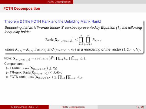
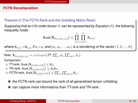
Theorem 2 (The FCTN Rank and the Unfolding Matrix Rank)
Supposing that an Nth-order tensor X can be represented by Equation (1), the followinginequality holds:
Rank(X[n1:d ;nd+1:N ]
)≤
d∏i=1
N∏j=d+1
Rni,nj ,
where Rni,nj =Rnj,ni if ni>nj and (n1, n2,· · ·, nN) is a reordering of the vector (1, 2,· · ·,N).
Note: X[n1:d ;nd+1:N ] = reshape(~X n,∏d
i=1 Ini ,∏N
i=d+1 Ini
).
Comparison: TT-rank: Rank
(X[1:d;d+1:N]
)≤ Rd;
TR-rank: Rank(X[1:d;d+1:N]
)≤ RdRN ;
FCTN-rank: Rank(X[1:d;d+1:N]
)≤∏d
i=1∏N
j=d+1 Ri,j.
the FCTN-rank can bound the rank of all generalized tensor unfolding;
can capture more informations than TT-rank and TR-rank;
Yu-Bang Zheng (UESTC) FCTN Decomposition 15 / 29
FCTN Decomposition
FCTN Decomposition
Theorem 2 (The FCTN Rank and the Unfolding Matrix Rank)
Supposing that an Nth-order tensor X can be represented by Equation (1), the followinginequality holds:
Rank(X[n1:d ;nd+1:N ]
)≤
d∏i=1
N∏j=d+1
Rni,nj ,
where Rni,nj =Rnj,ni if ni>nj and (n1, n2,· · ·, nN) is a reordering of the vector (1, 2,· · ·,N).
Note: X[n1:d ;nd+1:N ] = reshape(~X n,∏d
i=1 Ini ,∏N
i=d+1 Ini
).
Comparison: TT-rank: Rank
(X[1:d;d+1:N]
)≤ Rd;
TR-rank: Rank(X[1:d;d+1:N]
)≤ RdRN ;
FCTN-rank: Rank(X[1:d;d+1:N]
)≤∏d
i=1∏N
j=d+1 Ri,j.
the FCTN-rank can bound the rank of all generalized tensor unfolding;
can capture more informations than TT-rank and TR-rank;
Yu-Bang Zheng (UESTC) FCTN Decomposition 15 / 29
FCTN Decomposition
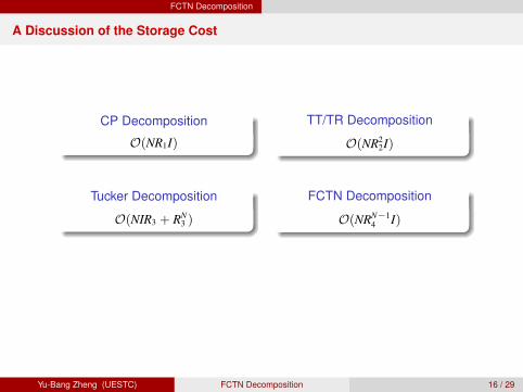
A Discussion of the Storage Cost
CP Decomposition
O(NR1I)
TT/TR Decomposition
O(NR22I)
Tucker Decomposition
O(NIR3 + RN3 )
FCTN Decomposition
O(NRN−14 I)
The storage cost of the FCTN decomposition seems to theoretical high. But when weexpress real-world data, the required FCTN-rank is usually less than CP, TT, TR, andTucker-ranks.
Yu-Bang Zheng (UESTC) FCTN Decomposition 16 / 29

FCTN Decomposition
A Discussion of the Storage Cost
CP Decomposition
O(NR1I)
TT/TR Decomposition
O(NR22I)
Tucker Decomposition
O(NIR3 + RN3 )
FCTN Decomposition
O(NRN−14 I)
The storage cost of the FCTN decomposition seems to theoretical high. But when weexpress real-world data, the required FCTN-rank is usually less than CP, TT, TR, andTucker-ranks.
Yu-Bang Zheng (UESTC) FCTN Decomposition 16 / 29
FCTN Decomposition
FCTN Composition
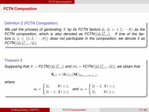
Definition 2 (FCTN Composition)
We call the process of generating X by its FCTN factors Gk (k = 1, 2, · · ·N) as theFCTN composition, which is also denoted as FCTN
(GkN
k=1
). If one of the fac-
tors Gt (t ∈ 1, 2, · · · ,N) does not participate in the composition, we denote it asFCTN
(GkN
k=1, /Gt)
Theorem 3
Supposing that X = FCTN(GkN
k=1
)andMt = FCTN
(GkN
k=1, /Gt), we obtain that
X(t) = (Gt)(t)(Mt)[m1:N−1;n1:N−1],
where
mi =
2i, if i < t,
2i− 1, if i ≥ t,and ni =
2i− 1, if i < t,
2i, if i ≥ t.
Yu-Bang Zheng (UESTC) FCTN Decomposition 17 / 29

FCTN-TC Model and Solving Algorithm
Outline
1 Background and Motivation
2 FCTN Decomposition
3 FCTN-TC Model and Solving Algorithm
4 Numerical Experiments
5 Conclusion
Yu-Bang Zheng (UESTC) FCTN Decomposition 18 / 29

FCTN-TC Model and Solving Algorithm
FCTN-TC Model
Incomplete Observation
F ∈ RI1×I2×···×IN
⇐ Relationship
PΩ(X ) = PΩ(F)⇒ Underlying Tensor
X ∈ RI1×I2×···×IN
⇓
FCTN Decomposition-Based TC (FCTN-TC) Model
minX ,G
12‖X − FCTN(G1,G2, · · · ,GN)‖2
F + ιS(X ), (2)
where G = (G1,G2,· · ·,GN),
ιS(X ) :=
0, if X ∈ S,∞, otherwise,
with S := X : PΩ(X − F)=0,
Ω is the index of the known elements, and PΩ(X ) is a projection operator which projectsthe elements in Ω to themselves and all others to zeros.
Yu-Bang Zheng (UESTC) FCTN Decomposition 19 / 29

FCTN-TC Model and Solving Algorithm
PAM-Based Algorithm
Proximal Alternating Minimization (PAM)G(s+1)
k =argminGk
f (G(s+1)
1:k−1 ,Gk,G(s)k+1:N ,X
(s)) +ρ
2‖Gk − G(s)
k ‖2F
, k=1, 2, · · ·,N,
X (s+1) =argminX
f (G(s+1),X ) +
ρ
2‖X − X (s)‖2
F
,
(3)
where f (G,X ) is the objective function of (2) and ρ > 0 is a proximal parameter.
Gk-Subproblems (k=1, 2, · · ·,N)
(G(s+1)k )(k) =
[X(s)
(k)(M(s)k )[n1:N−1;m1:N−1]+ρ(G(s)
k )(k)][
(M(s)k )[m1:N−1;n1:N−1](M(s)
k )[n1:N−1;m1:N−1]+ρI]−1
,
G(s+1)k = GenFold
((G(s+1)
k )(k), k; 1, · · · , k − 1, k + 1, · · · , N),
(4)
whereM(s)k =FCTN
(G(s+1)
1:k−1 ,Gk,G(s)k+1:N , /Gk
), and vectors m and n have the same setting as that in Theorem 3.
X -Subproblem
X (s+1)= PΩc
( FCTN(G(s+1)
k Nk=1
)+ ρX (s)
1 + ρ
)+ PΩ(F). (5)
Yu-Bang Zheng (UESTC) FCTN Decomposition 20 / 29

FCTN-TC Model and Solving Algorithm
PAM-Based Algorithm
Algorithm 1 PAM-Based Solver for the FCTN-TC Model.
Input: F ∈ RI1×I2×···×IN , Ω, the maximal FCTN-rank Rmax, and ρ = 0.1.Initialization: s = 0, smax = 1000, X (0) = F , the initial FCTN-rank R = maxones(N(N −
1)/2, 1),Rmax−5, and G(0)k = rand(R1,k,R2,k,· · ·,Rk−1,k, Ik,Rk,k+1,· · ·,Rk,N), where k=1, 2,· · ·,N.
while not converged and s < smax do
Update G(s+1)k via (4).
Update X (s+1) via (5).
Let R = minR + 1,Rmax and expand G(s+1)k if ‖X (s+1) −X (s)‖F/‖X (s)‖F < 10−2.
Check the convergence condition: ‖X (s+1) −X (s)‖F/‖X (s)‖F < 10−5.
Let s = s + 1.end while
Output: The reconstructed tensor X .
Theorem 4 (Convergence)The sequence G(s),X (s)s∈N obtained by the Algorithm 1 globally converges to a criti-cal point of (2).
Yu-Bang Zheng (UESTC) FCTN Decomposition 21 / 29

Numerical Experiments
Outline
1 Background and Motivation
2 FCTN Decomposition
3 FCTN-TC Model and Solving Algorithm
4 Numerical Experiments
5 Conclusion
Yu-Bang Zheng (UESTC) FCTN Decomposition 22 / 29
Numerical Experiments
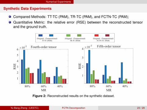
Synthetic Data Experiments
Compared Methods: TT-TC (PAM), TR-TC (PAM), and FCTN-TC (PAM);Quantitative Metric: the relative error (RSE) between the reconstructed tensorand the ground truth.
(Original) (Transpositional)
FCTN-TC (PAM)
(Original) (Transpositional)
TR-TC (PAM)
(Original) (Transpositional)
TT-TC (PAM)
Fourth-order tensor
80% 60% 40%
MR
1
2
3
4
5
6
RS
E
10-3 Fifth-order tensor
80% 60% 40%
MR
1
2
3
4
RS
E
10-3
Figure 2: Reconstructed results on the synthetic dataset.
Yu-Bang Zheng (UESTC) FCTN Decomposition 23 / 29

Numerical Experiments
Real Data Experiments
Compared Methods:
HaLRTC [Liu et al. 2013; IEEE TPAMI ];
TMac [Xu et al. 2015; IPI ];
t-SVD [Zhang and Aeron 2017; IEEE TSP ];
TMacTT [Bengua et al. 2017; IEEE TIP ];
TRLRF [Yuan et al. 2019; AAAI ].
Quantitative Metric:
PSNR;
RSE.
Yu-Bang Zheng (UESTC) FCTN Decomposition 24 / 29
Numerical Experiments
Color Video Data
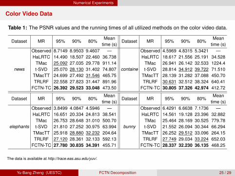
Table 1: The PSNR values and the running times of all utilized methods on the color video data.
Dataset MR 95% 90% 80%Mean
time (s)Dataset MR 95% 90% 80%
Meantime (s)
news
Observed 8.7149 8.9503 9.4607 —
containe
Observed 4.5969 4.8315 5.3421 —HaLRTC 14.490 18.507 22.460 36.738 HaLRTC 18.617 21.556 25.191 34.528
TMac 25.092 27.035 29.778 911.14 TMac 26.941 26.142 32.533 1224.4t-SVD 25.070 28.130 31.402 74.807 t-SVD 28.814 34.912 39.722 71.510
TMacTT 24.699 27.492 31.546 465.75 TMacTT 28.139 31.282 37.088 450.70TRLRF 22.558 27.823 31.447 891.96 TRLRF 30.631 32.512 38.324 640.41
FCTN-TC 26.392 29.523 33.048 473.50 FCTN-TC 30.805 37.326 42.974 412.72
Dataset MR 95% 90% 80%Mean
time (s)Dataset MR 95% 90% 80%
Meantime (s)
elephants
Observed 3.8499 4.0847 4.5946 —
bunny
Observed 6.4291 6.6638 7.1736 —HaLRTC 16.651 20.334 24.813 38.541 HaLRTC 14.561 19.128 23.396 32.882
TMac 26.753 28.648 31.010 500.70 TMac 25.464 28.169 30.525 779.78t-SVD 21.810 27.252 30.975 63.994 t-SVD 21.552 26.094 30.344 66.294
TMacTT 25.918 28.880 32.232 204.64 TMacTT 26.252 29.512 33.096 264.15TRLRF 27.120 28.361 32.133 592.13 TRLRF 27.749 29.034 33.224 652.03
FCTN-TC 27.780 30.835 34.391 455.71 FCTN-TC 28.337 32.230 36.135 468.25
The data is available at http://trace.eas.asu.edu/yuv/.
Yu-Bang Zheng (UESTC) FCTN Decomposition 25 / 29
Numerical Experiments
Color Video Data
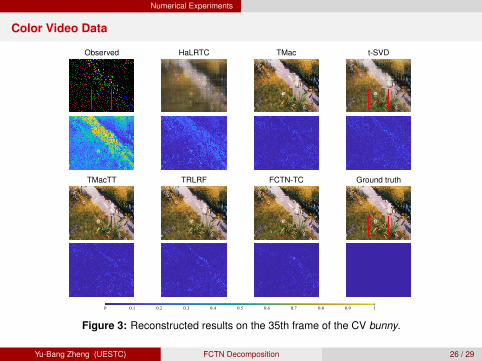
Observed HaLRTC TMac t-SVD
TMacTT TRLRF FCTN-TC Ground truth
0 0.1 0.2 0.3 0.4 0.5 0.6 0.7 0.8 0.9 1
0 0.40.3 0.70.5 0.80.2 0.60.1 10.9
Figure 3: Reconstructed results on the 35th frame of the CV bunny.
Yu-Bang Zheng (UESTC) FCTN Decomposition 26 / 29
Numerical Experiments
Traffic Data
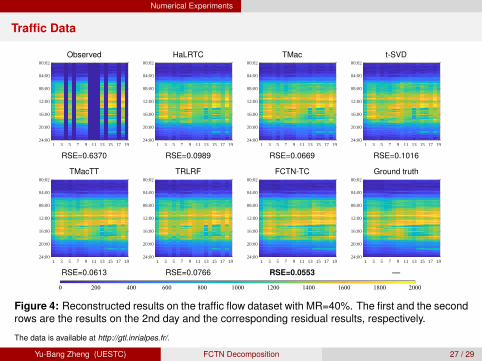
Observed HaLRTC TMac t-SVD
1 3 5 7 9 11 13 15 17 19
00:02
04:00
08:00
12:00
16:00
20:00
24:001 3 5 7 9 11 13 15 17 19
00:02
04:00
08:00
12:00
16:00
20:00
24:001 3 5 7 9 11 13 15 17 19
00:02
04:00
08:00
12:00
16:00
20:00
24:001 3 5 7 9 11 13 15 17 19
00:02
04:00
08:00
12:00
16:00
20:00
24:00
RSE=0.6370 RSE=0.0989 RSE=0.0669 RSE=0.1016
TMacTT TRLRF FCTN-TC Ground truth
1 3 5 7 9 11 13 15 17 19
00:02
04:00
08:00
12:00
16:00
20:00
24:001 3 5 7 9 11 13 15 17 19
00:02
04:00
08:00
12:00
16:00
20:00
24:001 3 5 7 9 11 13 15 17 19
00:02
04:00
08:00
12:00
16:00
20:00
24:001 3 5 7 9 11 13 15 17 19
00:02
04:00
08:00
12:00
16:00
20:00
24:00
RSE=0.0613 RSE=0.0766 RSE=0.0553 —
0 0.1 0.2 0.3 0.4 0.5 0.6 0.7 0.8 0.9 1
0 800600 14001000 1600400 1200200 20001800
Figure 4: Reconstructed results on the traffic flow dataset with MR=40%. The first and the secondrows are the results on the 2nd day and the corresponding residual results, respectively.
The data is available at http://gtl.inrialpes.fr/.
Yu-Bang Zheng (UESTC) FCTN Decomposition 27 / 29

Conclusion
Conclusion
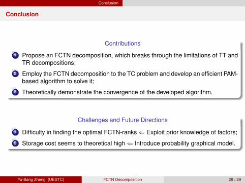
Contributions
1 Propose an FCTN decomposition, which breaks through the limitations of TT andTR decompositions;
2 Employ the FCTN decomposition to the TC problem and develop an efficient PAM-based algorithm to solve it;
3 Theoretically demonstrate the convergence of the developed algorithm.
Challenges and Future Directions
1 Difficulty in finding the optimal FCTN-ranks⇐ Exploit prior knowledge of factors;
2 Storage cost seems to theoretical high⇐ Introduce probability graphical model.
Yu-Bang Zheng (UESTC) FCTN Decomposition 28 / 29
Conclusion
Conclusion
Contributions
1 Propose an FCTN decomposition, which breaks through the limitations of TT andTR decompositions;
2 Employ the FCTN decomposition to the TC problem and develop an efficient PAM-based algorithm to solve it;
3 Theoretically demonstrate the convergence of the developed algorithm.
Challenges and Future Directions
1 Difficulty in finding the optimal FCTN-ranks⇐ Exploit prior knowledge of factors;
2 Storage cost seems to theoretical high⇐ Introduce probability graphical model.
Yu-Bang Zheng (UESTC) FCTN Decomposition 28 / 29

Conclusion
Thank you very much for listening!
Homepage: https://yubangzheng.github.io
Yu-Bang Zheng (UESTC) FCTN Decomposition 29 / 29


![Ranking Methods for Tensor Components Analysis and their ...cet/TieneFilisbino_sibgrapi13.pdf · [6], tensor discriminant analysis (TDA) [7], [8] and tensor rank-one decomposition](https://img.pdfslide.us/doc/110x75/5f78fbe48023322255060d71/ranking-methods-for-tensor-components-analysis-and-their-cettienefilisbino.jpg)


![Fourier PCA and Robust Tensor DecompositionarXiv:1306.5825v5 [cs.LG] 27 Jun 2014 Fourier PCA and Robust Tensor Decomposition NavinGoyal∗ SantoshVempala† YingXiao‡ July1,2014](https://img.pdfslide.us/doc/110x75/5f24bd9964c6ac1c9e07dd8b/fourier-pca-and-robust-tensor-decomposition-arxiv13065825v5-cslg-27-jun-2014.jpg)


![Probabilistic Streaming Tensor Decompositionzhe/pdf/POST.pdf · Probabilistic Streaming Tensor Decomposition Yishuai Du y, Yimin Zheng , Kuang-chih Lee], Shandian Zhey University](https://img.pdfslide.us/doc/110x75/5eb6be1e3d209031916fd245/probabilistic-streaming-tensor-decomposition-zhepdfpostpdf-probabilistic-streaming.jpg)