STATS 319: Literature of StatisticsThe Sum-of-Squares Algorithmic Paradigm in StatisticsInstructor: Tselil Schramm

Lecture 1January 25, 2021

Lecturer/Scribe: Kevin Tian

Tensor decomposition

In this lecture we will introduce the problem of tensor decomposition, discuss its usefulness as analgorithmic primitive in unsupervised learning, and give a general sum-of-squares framework for tensordecomposition. We will then show how to apply this framework to the problem of decomposing overcom-plete tensors with random components.

1 Tensor decomposition

Tensor decomposition is a high-order generalization of matrix decomposition, where we decompose atensor into rank-one factors. Formally, in the order-3 tensor decomposition problem, we are given thetensor T ∈ Rd1⊗d2⊗d3 , and we are promised that it has the form

T =n∑i=1

ai ⊗ bi ⊗ ci ,

for vectors ai ∈ Rd1 , bi ∈ Rd2 , ci ∈ Rd3 , which are called the components of the tensor. The order-3 tensordecomposition problem is to recover the components {ai , bi , ci}ni=1 given T. The minimum n for whichT can be decomposed in such a way is called the rank of T. Throughout this lecture we will treat thesymmetric case wherein ai = bi = ci for every i ∈ [n], though much of what we discuss can be generalizedto handle asymmetric (and higher-order) tensors as well.

We remark that many tensor-related problems such as computing rank or decomposition are NP-hardin the worst case, so typically we have to make some structural or distributional assumptions about T tohave a hope of solving the problem in polynomial time.

Uniqueness of decompositions and applications to parameter estimation. Low-rank matrix de-compositions are non-unique. Even a single rank-one factor uv⊤ can be rewritten as (Mu)(Mv)⊤ for anyunitary matrix M. We sometimes get around this symmetry by insisting on speci�c types of decompo-sitions, like the eigendecomposition or singular value decomposition, which we know are unique (up torepresentation of rank > 1 subspaces) by the spectral theorem.

Tensors, on the other hand, often enjoy a uniqueness of the minimum rank decompoisition even with-out such orthogonality conditions. Further, tensors may have unique decompositions even when the rankn exceeds the dimension d! This is what we refer to as the overcomplete setting (n > d).

This makes tensor decomposition a useful primitive for high-dimensional parameter estimation tasks.As a concrete example, consider learning the parameters of a mixture of spherical Gaussians,

= ∑i∈[k]

wi (�i ,1),

where {�i}i∈[k] ⊂ Rd , and w ∈ Δk is a probability distribution. A common paradigm for this problem is themethod of moments, where one takes enough samples to accurately estimate the order-k moments of thedistribution, and expresses them in terms of the parameters. For example, for X ∼ ,

E [X ] = ∑i∈[k]

wi�i , E [XX⊤] = ∑i∈[k]

wi�i�⊤i + 1.

1

However, even if we were given exact information about the second moment matrix E[XX⊤], this is notenough to learn the {wi , �i}i∈[k] because of the issue of rotation invariance of the matrix decomposition.Fortunately, the third-moment tensor can also be written in terms of the parameters of the distribution,and will let us extract information about ∑i∈[k] wi�⊗3i . Thus, we can use a tensor decomposition algorithmwill tell us the parameters of the mixture model. Many fundamental high-dimensional algorithmic tasksuse tensor decomposition as a basic stepping stone; we list a couple (without going into details):

1. Dictionary learning, where we have a dictionary A ∈ Rn×d and receive samples Av + � , wherev is sparse and � a noise vector. Here the goal is to learn the dictionary A. This is achieved byapproximately learning the polynomial ∑i∈[n] ⟨ai , u⟩

k from samples and then running a tensor de-composition algorithm.

2. Topic modeling. This is similar to dictionary learning (the columns represent “topics”), but furtherassumptions are made on the model (e.g. the combination vector v is non-negative).

3. Learning phylogenetic trees. Here the idea is that we can use some types of property tests to learnthe topology of the tree, at which point we can estimate moments of e.g. passing on genetic traits.This lets us learn the parameters of the tree from tensor decomposition, such as estimating transitionmatrices (from parent species to children species).

4. Independent component analysis (the “cocktail party problem”) where we wish to denoise a mixture.The problem formulation is quite similar to dictionary learning.

Notice that for these learning applications, it is much harder to collect enough samples to approximate thetrue order-k tensor as k gets very large (since there are dk entries), so it is ideal to learn the parameterse�ciently from a low-order tensor, such as order-3. However, it gets easier to design algorithms for tensordecomposition the more moments we have access to (as the next section demonstrates), which makes itimportant to understand algorithms for low-order tensors.

2 Jennrich’s algorithm

Now, we will discuss Jennrich’s algorithm, a simple algorithm for decomposing undercomplete tensors.Later, we will see how Jennrich’s algorithm is used, in combination with sum-of-squares relaxations, todecompose overcomplete tensors. For now, let T = ∑i∈[n] a⊗3i be a symmetric third-order tensor for con-creteness.

Orthonormal components. We �rst illustrate the main idea of Jennrich’s algorithm in a very simplesetting: suppose that the ai are orthonormal. In this case, the algorithm is just to sample g ∼ (0,1d ) andthen write down the matrix

Mg = T[g, ⋅, ⋅] ∶=d∑i=1

giTi

for Ti the ith d × d “slice” of T. We call such a matrix a “random contraction” of T. One can check that

Mg = ∑i∈[n]

⟨ai , g⟩ aia⊤i ,

and further when the Ai∶ are orthonormal, the {(⟨ai , g⟩, ai)}ni=1 are also the unique eigendecomposition ofMg with probability 1. So, by computing the eigendecomposition of Mg , we can recover the ai .

2

Independent components. Though we will not use it in what follows, we remark that a variation onthis works more generally when the {ai}i∈[n] are not necessarily orthonormal (or close to orthonormal),but merely linearly independent (so still n 6 d). The algorithm is as follows: we sample g, g′ ∼ (0,1d )independently, and form Mg ,Mg′ . Denoting Dg ∶= diag {⟨ai , g⟩}i∈[n], note that

Mg = U⊤DgU, Mg′ = U⊤Dg′U,

where the rows of U are given by the {ai}i∈[n]. Hence,

M−1g Mg′ = U−1 (D−1g Dg′)U.

Now for any matrix A = U−1DU with D diagonal, the rows of U are the eigenvectors of A (up to scaling),so we can use the eigendecomposition ofM−1

g Mg′ to recover the ai up to scaling, then solve a linear systemto recover the scales (so long as the ai are linearly independent the solution will be unique).

3 Running Jennrich on “lifted” tensors.

Recall that we are interested in overcomplete third-order tensor decomposition (say n ≫ d), so Jennrich’salgorithm does not work as-is. Suppose however that n 6 d2, Then though the ai are not linearly inde-pendent, the vectors a⊗2i ∈ Rd2 very well may be (for example, when the ai are chosen independently from (0, 1d1) or uniformly from Sd−1, the a⊗2i are linearly independent with probability 1).

Now, if we also had access to the sixth-order tensor in the components ∑i∈[n] a⊗6i , then thinking ofthis as a 3-tensor in the components a⊗2i ∈ Rd2 , we could form ∑i∈[n] ⟨a⊗2i , g⟩(a⊗2i ) (a⊗2i )

⊤ via a randomcontraction and use it to recover the {a⊗2i }i∈[n] as before.

In the learning applications we mentioned above, often times it is possible to obtain access to the order-6 tensor by estimating the order-6 moments; however as mentioned above, estimating higher-momenttensors is sample-intensive. So we would like a way to lift the third-order tensor to a sixth-order tensor,without needing any additional samples.

The following sections we will use sum-of-squares to “lift” a third-order tensor T to a surrogate for theorder-6 tensor. We will quantify when we can treat a “lifted” higher-order tensor as the true higher-ordertensor we want (the “signal”) plus additional information which will hopefully cancel for random instances(the “noise”). For this, it will be helpful to see a variation on Jennrich’s algorithm which succeeds whenthe tensor has the structure of being a rank-1 component in the presence of noise:

Noisy rank-1 tensor. We can generalize the above to the setting where we observe a rank-1 tensor withthe addition of some “well-behaved” noise. That is, we have T = a⊗3 + E, for E ∈ (Rd )⊗3 and a ∈ Rd (saythat we have scaled T so that a is a unit vector). We will show that in this case, the top eigenvector of arandom contraction of T is correlated with a with not-too-small a probability.

Lemma 3.1. If we are given T ∈ (Rd )⊗3 such that T = a⊗3 + E for a ∈ Rd a unit vector and E a symmetric3-tensor whose d2 × d reshaping E has ‖E‖op 6 � and Ea = 0,1 then for any " > 0, with probability at leastΩ(d−�2) over g ∼ (0,1d ), Furthermore,

Mg = � ⋅ aa⊤ + N ,

for N ∈ Rd×d with � > �� (1 − o(1)) ⋅ ‖N ‖op , so that if � > (1 + o(1))�, a is the top eigenvector ofMg .2

1This condition can in fact be relaxed, but it will signi�cantly simplify the proof.2If we loosen the requirement that Ea = 0, then a will instead be closely correlated to the top eigenvector.

3

Before proving the lemma, let us make a couple of observations. Firstly, with this lemma in hand,we have an algorithm for producing a list of vectors which, with high probability, includes a: we simplytry O(d (1+")�) independent random contractions of T, and �nd the top eigenvector of each. If we hada procedure for testing whether a vector v is indeed close to a, this would amount to a decompositionalgorithm.

Secondly, let us foreshadow how this lemma will be used in the context of sum-of-squares. Given anovercomplete 3-tensor T, we will write a properly constrained sum-of-squares program over indetermi-nates u ∈ Rd and solve for a pseudoexpectation operator E ∶ R[u]610 → R which will satisfy that theorder-6 pseudomoment tensor T6 = Eu⊗6 will in fact be of the form T6 = ∑m

i=1 a⊗6i + E, for E a 6-tensorwhose d4 × d2 reshapings have operator norm at most 1. Then, we will be able to run Jennrich’s algorithmpoly(d) times as a rounding algorithm on T6 to produce a list of vectors which contains a vector close toa⊗2i for each i ∈ [n], after which we will be able to design a testing procedure to �nd the true componentsai .

Proof of Lemma 3.1. We notice that

Mg =d∑i=1

gi ⋅ Ti =d∑i=1

gi ⋅ (a(i) ⋅ aa⊤ + Ei) = ⟨g, a⟩ ⋅ aa⊤ +d∑i=1

giEi .

Now, we can split g = ⟨a, g⟩a + ℎ for ⟨ℎ, a⟩ = 0. Notice that in fact ∑di=1 giEi = ∑d

i=1 ℎiEi , by the symmetryof E (as E[g, ⋅, ⋅] is simply a reshaping of E[⋅, ⋅, g] = Eg, and then applying linearity). So by the independenceof ℎ and ⟨g, a⟩, the quantities � = ⟨g, a⟩ and ‖∑d

i=1 giEi‖op are independent as well.3

Using a concentration inequality for Gaussian matrix series (see e.g. Theorem 1.2 in [Tro12]), we havethe following:

Claim 3.2.

Prg∼ (0,1) [

‖‖‖‖‖

d∑i=1

giEi‖‖‖‖‖op

> �√2(1 + �) log d

]6 d−� .

Furthermore, one can show that ⟨g, a⟩ ∼ (0, 1). So using a Gaussian anticoncentration statement,we have that Prg∼ (0,1)[⟨g, a⟩ >

√2(1 + ") log d] > Ω(d−(1+")).

Hence, with probability at least Ω(d−�2), we have that N = ∑di=1 giEi has ‖N ‖op 6 �

√2(1 + log d) and

� > �√2 log d hold simultaneously. This gives our �rst conclusion. For our second conclusion, we simply

notice that a is in the null space of N by our assumption that Ea = 0.

4 Rounding with Jennrich and pseudodistributions

The goal of this section is to answer the following question:

When is it possible to design a Jennrich-based rounding algorithm, when we only

have access to a pseudoexpectation operator in lieu of “true” moments?

In the previous section we saw that it would be helpful if we had access to the true sixth-moment tensorof the {ai}i∈[n]. In its place, we will only be able to obtain a pseudoexpectation operator subject to help-ful polynomial constraints which will allow us to apply Jennrich’s algorithm in the style of Lemma 3.1.

3In the case when we do not have independence but instead have a bound on, say, the norm ‖Ea‖, one can make a more carefulargument accounting for this, at the cost of some error terms.

4

Throughout this section we will be concerned with general conditions under which SoS can be used to de-compose an undercomplete tensor with components {bi}i∈[n].4 Ultimately, we will use our SOS frameworkto recover the {bi}i∈[n] via simulating higher moments.

We will prove Theorem 4.1 (based on Theorem 4.1 of [MSS16]), which is an SoS version of a variantof Lemma 3.1 (in the setting where � < 1 is small and without the stipulation that Ea = 0). In particular,Theorem 4.1 shows that as long as E is a degree-O(k) pseudoexpectation operator over a vector variableu ∈ Rd , satisfying for some unit vector b,

‖u‖22 6 1 and E [⟨b, u⟩k+2] = Ω(1

"√k)

‖‖‖E [uu⊤]

‖‖‖op, (1)

then with reasonable probability the top eigenvector of a contracted matrix (a random Gaussian contractionof the order-k + 2 pseudoexpectation) is 1 − O(") correlated with b.

Notice that if b1,… , bn ∈ Rd are unit vectors which are isotropic (Ei∼[n]bib⊤i ⪯ 1) and near-orthogonalso that |⟨bi , bj⟩| 6 � if i ≠ j,5 then taking Eu⊗k+2 to be the uniform mixture tensor Ei∼[n]b⊗k+2i , we have thatEuu⊤ ⪯ 1

n1, and

Ei∈[n]E[⟨u, bi⟩k+2] = Ei,j∼[n]⟨bi , bj⟩k+2 =1n± O(n�k+2).

In particular, if �k+2n ≪ 1n , then taking E to be consistent with the moments of the uniform mixture over

the bi , by an averaging argument there must exist some � ∈ [n] such that b = b� satis�es (1) so long ask = Ω( 1"2 ). So we will later use SoS to �nd a proxy for this moment tensor.

Theorem 4.1 (SoS version of Lemma 3.1). Let E be a degree-O(k) pseudoexpectation satisfying the conditions(1). Then with probability d−O(k) over the choice of the Gaussian vector g, the top eigenvector v ofMg satis�es⟨b, v⟩2 = 1 − O(").

Proof. For any vector v ∈ (Rd )⊗k , we will use the notation Mv ∶= E[⟨v, u⊗k⟩ ⋅ uu⊤] throughout.The Davis-Kahan theorem says that if M and unit vector b satisfy ‖‖M − bb⊤‖‖op 6 ", then their top

eigenvectors have correlation 1 − O("). Applying this theorem, we wish to show with probability d−O(k)

over g ∼ (0,1dk ), there is a multiple of Mg at most " away in operator norm from bb⊤. It will beconvenient for us to write an orthogonal decomposition of Mg by projecting g against b⊗k , via

Mg = �Mb⊗k +Mℎ, for ℎ ∶= g − ⟨g, b⊗k⟩ b⊗k and � ∶= ⟨g, b⊗k⟩ . (2)

Using Gaussian anticoncentration, with probability at least d−O(k), we have � = ⟨g, b⊗k⟩ >√k log d .

Conditioning on this event, and letting t = E [⟨b, u⟩k+2],

Eg [‖‖‖‖1�tMg − bb⊤

‖‖‖‖op

|||||� >

√k log d

]6

‖‖‖‖1tMb⊗k − bb

⊤‖‖‖‖op+ Eg [

1�t

‖Mℎ‖op

|||||⟨g, b⊗k⟩ >

√k log d

],

6‖‖‖‖1tMb⊗k − bb

⊤‖‖‖‖op+

1t√k log d

Eg [‖Mℎ‖op] , (3)

where we have used that ℎ is independent of �.Now, we will bound each term with a separate claim. We begin with the �rst term:

4It may be useful to keep in mind that these bi vectors which we wish to recover will be a polynomial transformation of theoriginal component vectors {ai}i∈[n] in the tensor decomposition, namely bi = a⊗2i for all i ∈ [n].

5This is satis�ed by random unit vectors with � = O( log n√d ) with high probability.

5

Claim 4.2. For t = E [⟨b, u⟩k+2],‖‖Mb⊗k − tbb

⊤‖‖op = O("t).

Proof. Let � = bb⊤ be the orthogonal projection onto the span of b; note �Mb⊗k� = tbb⊤. Since tΠ =ΠMb⊗kΠ, it su�ces for us to show that the operator norm of the left- and right-projections to the subspace(1 − Π) are small. That is,

‖‖Mb⊗k − tΠ‖‖op 6 2 ‖‖(1 − Π)Mb⊗kΠ‖‖op + ‖‖(1 − Π)Mb⊗kΠ(1 − Π)‖‖op

6 2 ‖‖�Mb⊗k�‖‖12op

‖‖(1 −�)Mb⊗k (1 −�)‖‖12op + ‖‖(1 −�)Mb⊗k (1 −�)‖‖op ,

(4)

Where we have used the triangle inequality in the �rst line and in the second line the Cauchy-Schwarzinequality in Mb⊗k which is positive semide�nite for even k. Next, we bound the operator norm of Mb⊗k

outside of �:

‖‖(1 −�)Mb⊗k (1 −�)‖‖op =‖‖‖E [⟨b, u⟩

k (1 −�)uu⊤(1 −�)]‖‖‖op

6 ‖‖‖E [⟨b, u⟩k (1 − ⟨b, u⟩2)]

‖‖‖op

62

k − 2E [⟨b, u⟩2] 6

2k − 2

‖‖‖E [uu⊤]

‖‖‖op.

Here, we used that ‖u‖2 6 1 is a polynomial constraint, and the inequality xk−2(1 − x2) 6 2k−2 , which has a

degree-O(k) SOS proof. Furthermore, observe that �Mb⊗k� ⪯ Mb⊗k ⪯ E [uu⊤], and all steps are certi�ableby degree-O(k) SOS. Going back to (4),

‖‖Mb⊗k − tbb⊤‖‖op 6

(2

k − 2+ 2

√2

k − 2)‖‖‖E [uu

⊤]‖‖‖op

= O("t).

In the last step we used the assumption (1).

Now, to bound the second term, we show that ‖Mℎ‖op is not too large in expectation.

Claim 4.3. For t = E [⟨b, u⟩k+2],

Eg [‖Mℎ‖op] = O ("t√k log d) .

Proof. For any pseudoexpectation respecting ‖u‖22 6 1,

Eg [‖Mℎ‖op] = Eg [

dk

∑j=1

ℎj ⋅ (u⊗k)j ⋅ uu⊤]= O (

√k log d)

‖‖‖E [u⊗k+1u⊤]

‖‖‖op= O (

√k log d)

‖‖‖E [uu⊤]

‖‖‖op,

Where the �rst equality again uses concentration of Gaussian matrix series ([Tro12], Theorem 1.2),6 andthe second equality uses that ‖Eu⊗k+1u⊤‖op 6 ‖Euu⊤‖op for any degree-4(k +2) pseudoexpectation operator(proof can be found in [MSS16], Theorem 6.1). The conclusion is immediate upon applying the condition(1).

Plugging Claims 4.2 and 4.3 into (3) and applying Markov’s inequality concludes the proof.6Because ℎ is not a standard normal vector one has to be careful here; however, one can show that using ℎ in place of g actually

improves the bound.

6

5 SOS framework for tensor decomposition

We are now ready to give an algorithm which uses Theorem 4.1 in an SOS framework for tensor decom-position. Here we will show that as long as our SoS relaxation satis�es the constraint7

n∑i=1

⟨bi , u⟩4 > 1 − "

(as well as ‖u‖2 6 1), Jennrich’s algorithm will recover a list of vectors, one of which is close to somecomponent bi . In the tensor decomposition algorithm of Ma Shi and Steurer [MSS16], one can recoverapproximations to all of the components by additionally using an SoS relaxation to (1) test if each recoveredvector is indeed close to some bi , and (2) after recovering some bi , one re-solve the SoS SDP with the addedcondition ⟨bi , u⟩2 < 0.01 to make sure that the next component which is found is far from bi .

Now, we can state the algorithm and give its analysis in the following theorem. At a high level, theSoS relaxation will look for an order-k tensor that is close to the moments of the uniform mixture overb1 = P (a1)⊗k , b2 = P (a2)⊗k ,… , bn = P (an)⊗k , for k a su�ciently large integer. The map P is intended toensure that P (ai) are linearly independent and close to orthonormal. It might be helpful to keep in mindthe example P (u) = u⊗2, which as discussed above lifts n 6 d2 vectors in d dimensions into d2 dimensionswhere they may be linearly independent.8 Then, Jennrich’s algorithm is run on the pseudomoment tensorEP (u)⊗k+2 to �nd a vector v which may be correlated with bi = P (ai) for one of the ai .

Theorem 5.1 (SoS Algorithm for recovering one lifted tensor component). Let P ∶ Rd → Rd′ be a degree-

O(k) lifting polynomial, for k ≪ 1" . For a set of vectors {ai}i∈[n], de�ne for all i ∈ [n], bi = P (ai), and suppose

all ‖bi‖2 > 1 − " and ‖‖‖∑i∈[n] bib⊤i‖‖‖op

6 1 + ". Finally, let be any polynomial system of inequalities which

implies

⊢O(k)

{

∑i∈[n]

⟨bi , P (u)⟩4 > (1 − ") ‖P (u)‖4}

. (5)

Then, consider the following algorithm, taking as input and P .

1. Compute a degree-O(k) pseudoexpectation E satisfying the constraints

∪{‖P (u)‖22 ∈ [1 − ", 1]

}, ‖‖‖E [P (u)P (u)

⊤]‖‖‖op

61 + "n

. (6)

2. For t ∈ [T ] with t = dO(k):

(a) Let g(t) ∼ (0,1⊗kd ), and compute the top eigenvector vt of

E [⟨g(t), P (u)⊗k⟩ P (u)P (u)⊤] .

(b) Add vt to the list of potential vectors which correlate with some bi .

3. Output the list {vt}t∈[T ].

7Notice that we may not know the entries of ∑ni=1 b⊗4i , so we will later have to make sure that this constraint is implied by

constraints that we can add.8However, sometimes ∑(a⊗2i )(a⊗2i ) may have a large operator norm, in which case it is helpful to make P more complicated

(e.g. P (u) = Πu⊗2 for a matrix Π that projects away from the span of large eigenvectors).

7

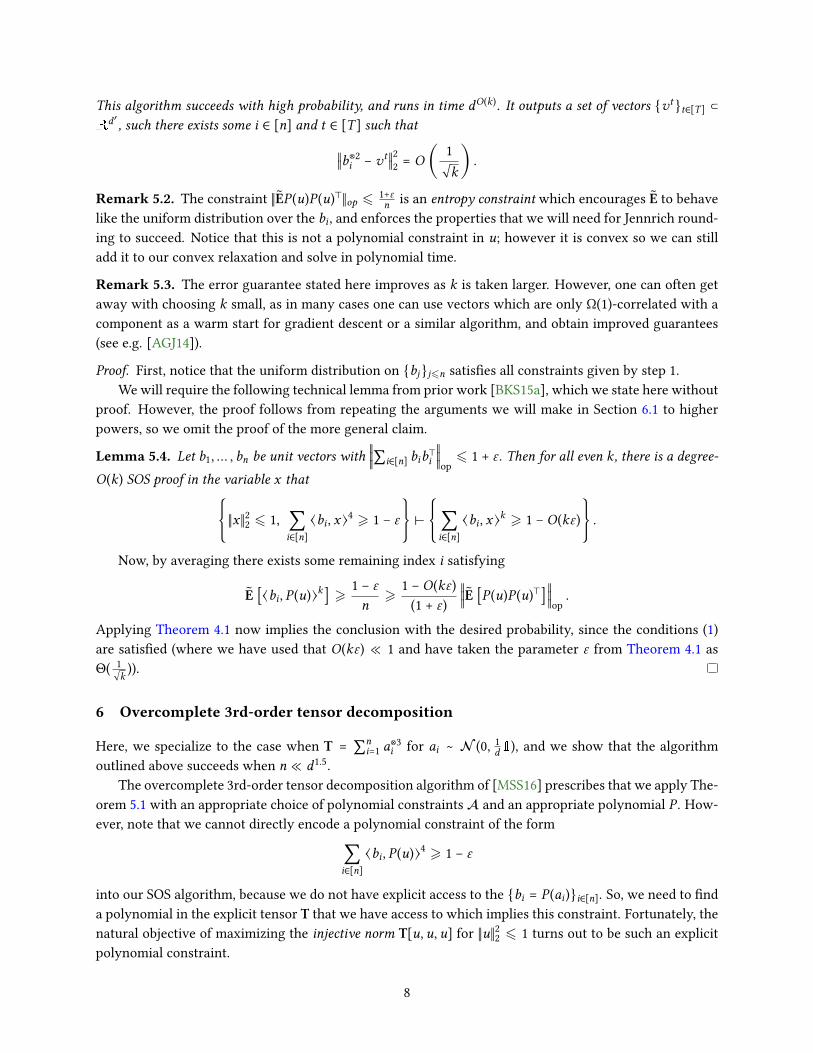
This algorithm succeeds with high probability, and runs in time dO(k). It outputs a set of vectors {vt}t∈[T ] ⊂Rd′ , such there exists some i ∈ [n] and t ∈ [T ] such that

‖‖b⊗2i − vt ‖‖

22 = O(

1√k)

.

Remark 5.2. The constraint ‖EP (u)P (u)⊤‖op 6 1+"n is an entropy constraint which encourages E to behave

like the uniform distribution over the bi , and enforces the properties that we will need for Jennrich round-ing to succeed. Notice that this is not a polynomial constraint in u; however it is convex so we can stilladd it to our convex relaxation and solve in polynomial time.

Remark 5.3. The error guarantee stated here improves as k is taken larger. However, one can often getaway with choosing k small, as in many cases one can use vectors which are only Ω(1)-correlated with acomponent as a warm start for gradient descent or a similar algorithm, and obtain improved guarantees(see e.g. [AGJ14]).

Proof. First, notice that the uniform distribution on {bj}j6n satis�es all constraints given by step 1.We will require the following technical lemma from prior work [BKS15a], which we state here without

proof. However, the proof follows from repeating the arguments we will make in Section 6.1 to higherpowers, so we omit the proof of the more general claim.

Lemma 5.4. Let b1,… , bn be unit vectors with‖‖‖∑i∈[n] bib⊤i

‖‖‖op6 1 + ". Then for all even k, there is a degree-

O(k) SOS proof in the variable x that{

‖x‖22 6 1, ∑i∈[n]

⟨bi , x⟩4 > 1 − "

}

⊢

{

∑i∈[n]

⟨bi , x⟩k > 1 − O(k")

}

.

Now, by averaging there exists some remaining index i satisfying

E [⟨bi , P (u)⟩k] >1 − "n

>1 − O(k")(1 + ")

‖‖‖E [P (u)P (u)⊤]

‖‖‖op.

Applying Theorem 4.1 now implies the conclusion with the desired probability, since the conditions (1)are satis�ed (where we have used that O(k") ≪ 1 and have taken the parameter " from Theorem 4.1 asΘ( 1√k )).

6 Overcomplete 3rd-order tensor decomposition

Here, we specialize to the case when T = ∑ni=1 a⊗3i for ai ∼ (0, 1d1), and we show that the algorithm

outlined above succeeds when n ≪ d1.5.The overcomplete 3rd-order tensor decomposition algorithm of [MSS16] prescribes that we apply The-

orem 5.1 with an appropriate choice of polynomial constraints and an appropriate polynomial P . How-ever, note that we cannot directly encode a polynomial constraint of the form

∑i∈[n]

⟨bi , P (u)⟩4 > 1 − "

into our SOS algorithm, because we do not have explicit access to the {bi = P (ai)}i∈[n]. So, we need to �nda polynomial in the explicit tensor T that we have access to which implies this constraint. Fortunately, thenatural objective of maximizing the injective norm T[u, u, u] for ‖u‖22 6 1 turns out to be such an explicitpolynomial constraint.

8

6.1 Maximizing the injective norm

This section is based on [GM15]. We present an observation that ‖T‖inj ∶= sup‖v‖2=1 T[v, v, v] is maximizedwhen v has large correlation with some ai as long as n ≪ d1.5. As we will see, this will imply that if we addthe constraint T[u, u, u] > 1 − " to our SoS relaxation, this will imply that ∑n

i=1⟨bi , u⊗2⟩ > 1 − "′. Observe

(T[u, u, u])2 =(

∑i∈[n]

⟨ai , u⟩3)

2

=(⟨

∑i∈[n]

⟨ai , u⟩2 ai , u⟩)

2

6‖‖‖‖‖‖∑i∈[n]

⟨ai , u⟩2 ai‖‖‖‖‖‖

2

2

‖u‖22

= ∑i∈[n]

⟨ai , u⟩4 ‖ai‖22 + ∑i≠j∈[n]

⟨ai , aj⟩ ⟨ai , u⟩2 ⟨aj , u⟩2 for all ‖u‖22 = 1.

(7)

We bound the two terms in (7) in two di�erent ways. Roughly speaking, the �rst term is reduced bysimilar Cauchy-Schwarz arguments as have already been used to understanding the operator norm of adegree-6 matrix in the components, and the operator norm of ∑i∈[n] aia⊤i , both of which follow straight-forwardly from concentration. The second term is captured by nested applications of matrix Bernsteinafter symmetrization.

6.1.1 2-to-4 norm

We consider the �rst term in (7), namely ∑i∈[n] ⟨ai , u⟩4 ‖ai‖22.

Lemma 6.1. There is a degree-O(1) SoS proof in the variables u ∈ Rd that

∑i∈[n]

⟨ai , u⟩4 ‖ai‖22 6 1 + O(1√d+n2

d3).

Proof. We use the following assumption, which can be shown via standard concentration arguments tohold with high probability for ai ∼ (0, 1d1).

Assumption 6.2. The vectors {ai}i∈[n] satisfy the following bounds.1. ⟨ai , aj⟩

26 O ( 1d ) for all i ≠ j ∈ [n].

2. ‖ai‖22 ∈ 1 ± O (1√d) for all i ∈ [n].

To bound the �rst term of (7), we use the same sequence of Cauchy-Schwarz inequalities:

(∑i∈[n]

⟨ai , u⟩4)

2

=(⟨

∑i∈[n]

⟨ai , u⟩3 ai , u⟩)

2

6‖‖‖‖‖‖∑i∈[n]

⟨ai , u⟩3 ai‖‖‖‖‖‖

2

2

= ∑i∈[n]

⟨ai , u⟩6 ‖ai‖22 + ∑i≠j∈[n]

⟨ai , aj⟩ ⟨ai , u⟩3 ⟨aj , u⟩3 .

(8)

Let A1 be the matrix whose rows are the {a⊗3i }i∈[n]. Then letting y = u⊗3 we have ‖A1‖22 = ∑i∈[n] ⟨ai , u⟩6. It

su�ces to bound the operator norm of A⊤1A1; note that it has entries

[A1]ij =

{‖ai‖62 i = j

⟨ai , aj⟩3 i ≠ j

.

9

By Assumption 6.2 and the Gershgorin disk theorem, the operator norm is bounded by 1 + O ( nd1.5 ). Note

that the Gershgorin strategy is only able to capture this fact with degree 6 polynomials. Next, we boundthe second term of (8):

(∑

i≠j∈[n]⟨ai , aj⟩ ⟨ai , u⟩3 ⟨aj , u⟩

3

)

2

6(

∑i≠j∈[n]

⟨ai , aj⟩2 ⟨ai , u⟩2 ⟨aj , u⟩

2

)(∑

i≠j∈[n]⟨ai , u⟩4 ⟨aj , u⟩

4

)

6 O (1d )(

∑i∈[n]

⟨ai , u⟩2)

2

(∑i∈[n]

⟨ai , u⟩4)

2

6 O(n2

d3).

Here, we used that the random matrix ∑i∈[n] aia⊤i has operator norm O ( nd ) with high probability. Thisconcludes the proof.

6.1.2 Cross terms

Lemma 6.3. There is a degree-O(1) SoS proof in the variabes u ∈ Rd that

∑i≠j∈[n]

⟨ai , aj⟩ ⟨ai , u⟩2 ⟨aj , u⟩26 O (

nd1.5)

.

Proof. To handle the cross terms of (7), namely ∑i≠j∈[n] ⟨ai , aj⟩ ⟨ai , u⟩2 ⟨aj , u⟩2, we observe that this is

the quadratic form of u⊗2 in the matrix A2 ∶= ∑i≠j∈[n] ⟨ai , aj⟩ (ai ⊗ aj)(ai ⊗ aj)⊤, so it su�ces to bound theoperator norm of A2. Letting {�i}i∈[n] be random signs, we have (in distribution) that

A2 = ∑i≠j∈[n]

�i�j ⟨ai , aj⟩ (ai ⊗ aj)(ai ⊗ aj)⊤.

Letting {� ′i }i∈[n] be independent random signs, Theorem 1 of [PMS95] says the concentration of A2 in anynorm is up to constants the same as concentration of

A′2 = ∑i≠j∈[n]

�i� ′j ⟨ai , aj⟩ (ai ⊗ aj)(ai ⊗ aj)⊤ = ∑

i∈[n]�i (

∑j∈[n],j≠i

� ′j ⟨ai , aj⟩ (ai ⊗ aj)(ai ⊗ aj)⊤

).

We use this symmetrization trick so we can apply matrix Bernstein twice toA′2 to bound its operator norm.Consider one term of A′2, which can be written as (�iaia⊤i ) ⊗ (∑j∈[n],j≠i � ′j ⟨ai , aj⟩ aja⊤j ). We apply matrixBernstein to ∑j∈[n],j≠i � ′j ⟨ai , aj⟩ aja⊤j , which requires an operator norm bound on individual terms and asecond moment bound. Under Assumption 6.2, each � ′j ⟨ai , aj⟩ aja⊤j is operator norm bounded by O( 1√

d ),and

∑j∈[n],j≠i

⟨ai , aj⟩2 ‖‖aj‖‖

22 aja

⊤j ⪯ O (

nd2)

1.

Thus, we conclude with high probability that each

(aia⊤i ) ⊗(∑

j∈[n],j≠i� ′j ⟨ai , aj⟩ aja

⊤j )

⪯ O(

√nd ) (aia⊤i ) ⊗ 1.

Next, we use matrix Bernstein once more on the random sum∑i∈[n] �iaia⊤i . Note that the termwise operatornorm bound is tightly concentrated near 1 and the second moment bound is the operator norm bound of∑i∈[n] aia⊤i which is O( nd ). Hence, the random sum ∑i∈[n] �iaia⊤i is bounded by O (

√ nd ). Combining these,

we have the following conclusion.

10

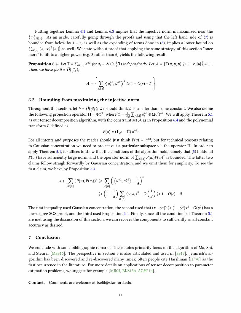
Putting together Lemma 6.1 and Lemma 6.3 implies that the injective norm is maximized near the{ai}i∈[n]. As an aside, carefully going through the proofs and using that the left hand side of (7) isbounded from below by 1 − ", as well as the expanding of terms done in (8), implies a lower bound on∑i∈[n] ⟨ai , x⟩

6 ‖ai‖22 as well. We state without proof that applying the same strategy of this section “oncemore” to lift to a higher power (e.g. 8 rather than 6) yields the following result.

Proposition 6.4. Let T = ∑i∈[n] a⊗3i for ai ∼ (0, 1d1) independently. Let = {T(u, u, u) > 1 − ", ‖u‖22 = 1}.Then, we have for � = O( n

d1.5 ),

⊢

{

∑i∈[n]

⟨a⊗2i , u⊗2⟩

4> 1 − O(") − �.

}

6.2 Rounding from maximizing the injective norm

Throughout this section, let � = O( nd1.5 ); we should think � is smaller than some constant. We also de�ne

the following projection operator � = ΦΦ⊤, where Φ = 1√d ∑j∈[d] e⊗2i ∈ (Rd )⊗2. We will apply Theorem 5.1

as our tensor decomposition algorithm, with the constraint set as in Proposition 6.4 and the polynomialtransform P de�ned as

P (a) = (1d2 −�) a⊗2.

For all intents and purposes the reader should just think P (a) = a⊗2, but for technical reasons relatingto Gaussian concentration we need to project out a particular subspace via the operator �. In order toapply Theorem 5.1, it su�ces to show that the conditions of the algorithm hold, namely that (5) holds, allP (ai) have su�ciently large norm, and the operator norm of ∑i∈[n] P (ai)P (ai)⊤ is bounded. The latter twoclaims follow straightforwardly by Gaussian concentration, and we omit them for simplicity. To see the�rst claim, we have by Proposition 6.4

⊢ ∑i∈[n]

⟨P (u), P (ai)⟩4 > ∑i∈[n]

(⟨u⊗2, a⊗2i ⟩ −

1d )

4

> (1 −1d )

∑i∈[n]

⟨u, ai⟩8 − O (1d )

> 1 − O(") − �.

The �rst inequality used Gaussian concentration, the second used that (x − y2)4 > (1 − y2)x4 −O(y2) has alow-degree SOS proof, and the third used Proposition 6.4. Finally, since all the conditions of Theorem 5.1are met using the discussion of this section, we can recover the components to su�ciently small constantaccuracy as desired.

7 Conclusion

We conclude with some bibliographic remarks. These notes primarily focus on the algorithm of Ma, Shi,and Steurer [MSS16]. The perspective in section 3 is also articulated and used in [SS17]. Jennrich’s al-gorithm has been discovered and re-discovered many times; often people cite Harshman [H+70] as the�rst occurrence in the literature. For more details on applications of tensor decomposition to parameterestimation problems, we suggest for example [MR05, BKS15b, AGH+14].

Contact. Comments are welcome at tselil@stanford.edu.

11

References

[AGH+14] A Anandkumar, R Ge, D Hsu, SM Kakade, and M Telgarsky. Tensor decompositions for learninglatent variable models. Journal of Machine Learning Research, 15:2773–2832, 2014. 11

[AGJ14] Animashree Anandkumar, Rong Ge, and Majid Janzamin. Guaranteed non-orthogonal tensordecomposition via alternating rank-1 updates. CoRR, abs/1402.5180, 2014. 8

[BKS15a] Boaz Barak, Jonathan A. Kelner, and David Steurer. Dictionary learning and tensor decom-position via the sum-of-squares method. In Proceedings of the Forty-Seventh Annual ACM onSymposium on Theory of Computing, STOC 2015, Portland, OR, USA, June 14-17, 2015, pages143–151, 2015. 8

[BKS15b] Boaz Barak, Jonathan A Kelner, and David Steurer. Dictionary learning and tensor decomposi-tion via the sum-of-squares method. In Proceedings of the forty-seventh annual ACM symposiumon Theory of computing, pages 143–151, 2015. 11

[GM15] Rong Ge and Tengyu Ma. Decomposing overcomplete 3rd order tensors using sum-of-squaresalgorithms. In Approximation, Randomization, and Combinatorial Optimization. Algorithms andTechniques, APPROX/RANDOM 2015, August 24-26, 2015, Princeton, NJ, USA, pages 829–849,2015. 9

[H+70] Richard A Harshman et al. Foundations of the parafac procedure: Models and conditions foran" explanatory" multimodal factor analysis. 1970. 11

[MR05] Elchanan Mossel and Sébastien Roch. Learning nonsingular phylogenies and hidden markovmodels. In Proceedings of the thirty-seventh annual ACM symposium on Theory of computing,pages 366–375, 2005. 11

[MSS16] Tengyu Ma, Jonathan Shi, and David Steurer. Polynomial-time tensor decompositions withsum-of-squares. In IEEE 57th Annual Symposium on Foundations of Computer Science, FOCS2016, 9-11 October 2016, Hyatt Regency, New Brunswick, New Jersey, USA, pages 438–446, 2016.5, 6, 7, 8, 11

[SS17] Tselil Schramm and David Steurer. Fast and robust tensor decomposition with applications todictionary learning. In Conference on Learning Theory, pages 1760–1793. PMLR, 2017. 11

[Tro12] Joel A Tropp. User-friendly tail bounds for sums of random matrices. Foundations of computa-tional mathematics, 12(4):389–434, 2012. 4, 6

12