TENSOR COMPLETION THROUGH MULTIPLE KRONECKER PRODUCT

DECOMPOSITION

Anh-Huy Phan1, Andrzej Cichocki1∗, Petr Tichavsky2†, Gheorghe Luta3, Austin Brockmeier4

1Brain Science Institute, RIKEN, Wakoshi, Japan2Institute of Information Theory and Automation, Prague, Czech Republic

3Department of Biostatistics, Bioinformatics, and Biomathematics,

Georgetown University, Washington, D.C., USA4Department of Electrical and Computer Engineering, University of Florida, Gainesville, FL, USA.

ABSTRACT

We propose a novel decomposition approach to impute missing val-

ues in tensor data. The method uses smaller scale multiway patches

to model the whole data or a small volume encompassing the ob-

served missing entries. Simulations on color images show that our

method can recover color images using only 5-10% of pixels, and

outperforms other available tensor completion methods.

Index Terms— tensor decomposition, tensor completion,

Kronecker tensor decomposition (KTD), color image

1. PROBLEM FORMULATION AND RELATED

WORK

Tensor decompositions have become a valuable tool for anal-

ysis of modern data with multiple modes. The approach has

found numerous areas of application such as in chemometrics,

telecommunication, analysis of fMRI data, time-varying EEG

spectrum, data mining, classification, clustering and compres-

sion [1–3]. For real-world and possibly large scale data, miss-

ing values may appear during data acquisition and transfor-

mation. In practice, a part of data, which does not conform

to the generative model, can be treated as missing. For ex-

ample, in decomposition of fluorescence data [1], data entries

corresponding to Rayleigh scatter emission do not conform to

the trilinear CANDECOMP/PARAFAC (CP) model. Hence,

they are often treated as missing, so that the fitted model is

not skewed by them [1]. Moreover, for relatively large data,

treating entries as missing can be considered as data sampling,

which is similar to using fiber sampling [4] to reduce the data

size, but to avoid severely decreasing the quality of the de-

composition. There are two major aims when analyzing such

incomplete data. One is to extract latent variables through de-

composition of the data tensor while discarding the missing

values [1, 5]. The other is to predict missing entries based on

complete data [6,7]. Note that the latter problem can be done

∗Also affiliated with the E.E. Dept., Warsaw University of Technology

and with Systems Research Institute, Polish Academy of Science, Poland.†The work of P. Tichavsky was supported by Grant Agency of the Czech

Republic through the project 102/09/1278.

using the approximate tensor from the former problem. Con-

versely, the quality of estimated hidden components in the

first problem can be improved with data completion.

Low-rank approximations are common approaches to

impute missing values [8, 9]. The truncated singular value

decomposition (SVD) of the matrix data is widely employed

with a soft-threshold and/or additional constraints such as

minimization of the nuclear norm [9, 10]. The problem is

also related to image inpainting which is often solved using

iterative shrinkage/thresholding (IST) algorithm [11,12]. The

considered problem also has connection to compressed sens-

ing [13–15]. For multiway data, CANDECOMP/PARAFAC

and Tucker decompositions [16–18] are the most common

tensor decompositions. On the basis of estimated factor ma-

trices, missing values can be heuristically imputed [5,19,20].

As the algorithms are not exclusively designed for data com-

pletion, such decompositions can result in overfitting.

In general, we can apply matrix completion techniques to

the unfolded version of the tensor data. However, since this

method only exploits spatial dependencies between data en-

tries along two modes, it may produce artifacts. Proper meth-

ods should address the structures of tensor data in higher or-

der such as the algorithms proposed in [6, 7, 21]. J. Liu et al.

solved the problem of low rank tensor completion extended

from that for matrix completion [9, 10], by employing block

coordinate descent to minimize the tensor trace norm. In [6],

S. Gandy et. al. considered the n-rank of a tensor as a sparsity

measure for the low-rank tensor recovery problem, and min-

imized the nuclear norm optimization problem based on the

Douglas-Rachford splitting technique [22]. In this direction,

we propose a novel method to impute missing values using

smaller scale multiway patches to model the whole data ten-

sor or a small volume comprising the observed missing en-

tries. Patches are used as dictionary for the construction of

the data. Small patches explain details of the tensor, while

large patterns capture the background. From the view point

of estimation of basis patterns, the decomposition is similar

to a dictionary learning problem in which the training data

is taken from contiguous non-overlapping patches. The pro-

3233978-1-4799-0356-6/13/$31.00 ©2013 IEEE ICASSP 2013

»

Ä

+

Ä

Ä Ä+¼

Y1b=

Y2

Y3

=

= ÄY3

= Ä

Y

Y1 YP

A1 X1AP XP

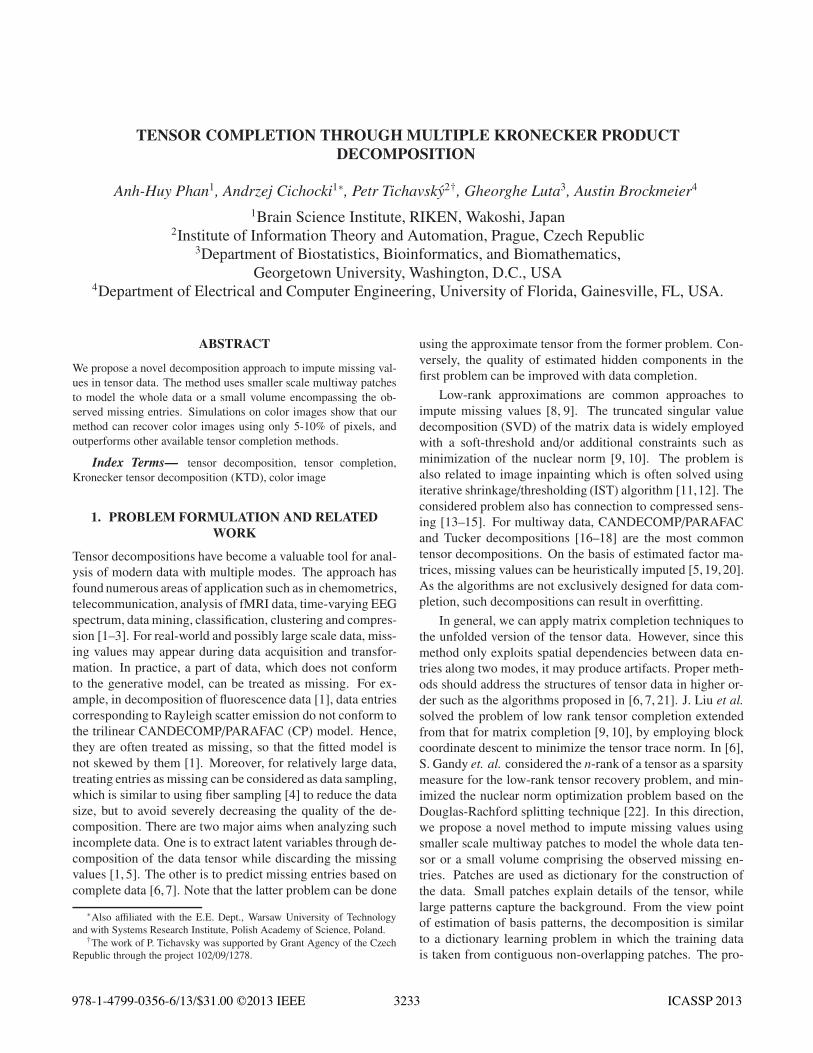
Fig. 1. Illustration of the tensor decomposition of an order-3 tensor

Y ∈ RI1×I2×I3 into P terms of Kronecker tensor products of Ap, Xp.

posed method is related to that for matrix data without miss-

ing entries in [24] and that for image restoration in [25, 26].

The method is an extension of the tensor decomposition

into multiple Kronecker products (KTD) [23] for incomplete

tensor data and with additional constraints to control the in-

tensity patterns. Moreover, a shifted decomposition is intro-

duced to efficiently improve the approximation. Simulations

on color images show that we can recover data while main-

taining perceptually good picture quality, even when using

only 5% of the data entries. The proposed algorithm was

compared with the LRTC [7] and C-SALSA [12] algorithms.

2. LEARNING STRUCTURAL PATTERNS FOR

INCOMPLETE DATA

We consider a multiway data Y of size I1 × I2 × · · · × IN with

missing entries indicated by a tensor W which is of the same

dimension as Y, and with binary values (0 if missing, and 1

if available). The task is to seek self-replicating structures

expressed by multiway patches (patterns) tiling the whole or

part of the data tensor Y (as illustrated in Fig. 1) so that the

following cost is minimized [23]

ϕ({Ap,Xp}) =1

2

∥

∥

∥

∥

∥

∥

∥

∥

W ⊛

Y −

P∑

p=1

Ap ⊗Xp

∥

∥

∥

∥

∥

∥

∥

∥

2

F

, (1)

where ⊛ stands for the Hadamard product, Ap ⊗ Xp denotes

the generalized Kronecker product between two tensors Ap

and Xp (see Defintion 1 and [23]). We term sub-tensors Xp of

size Kp1 × Kp2 × · · · × KpN with ‖Xp‖F = 1 as patterns, while

Ap of dimensions Jp1 × Jp2 × · · ·× JpN such that In = Jpn Kpn,

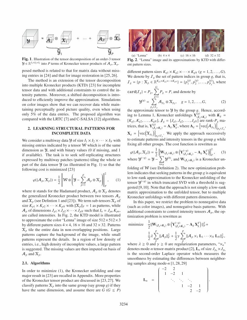
are called intensities. In Fig. 2, the KTD model is illustrated

to approximate the color “Lenna” image of size 512×512×3

by different pattern sizes 4 × 4, 16 × 16 and 32 × 32. Patterns

Xp tile the entire data in non-overlapping positions. Large

patterns capture the background of the image, while small

patterns represent the details. In a region of low density of

entries, i.e., high density of incomplete values, a large pattern

is suggested. The missing values are then imputed on basis of

Ap and Xp.

2.1. Algorithms

In order to minimize (1), the Kronecker unfolding and one

major result in [23] are recalled in Appendix. More properties

of the Kronecker tensor product are discussed in [23,27]. We

classify patterns Xp into the same group (say group g) if they

have the same dimension, and assume there are G (G ≤ P)

(a) “Lenna” (b) 4 × 4 (c) 16 × 16 (d) 32 × 32

Fig. 2. “Lenna” image and its approximations by KTD with differ-

ent pattern sizes.

different pattern sizes Kg1 × Kg2 × · · · × KgN (g = 1, 2, . . . ,G).

We denote by Ig the set of pattern indices in group g, that is,

Ig = {p : Xp ∈ RKg1×Kg2×···×KgN } = {p

(g)

1, p

(g)

2, . . . , p

(g)

Pg}, where

card{Ig} = Pg,

G∑

g=1

Pg = P, and denote by

Y(g)=∑

pg∈Ig

Apg⊗Xpg

, g = 1, 2, . . . ,G, (2)

the approximate tensor to Y by the group g. Hence, accord-

ing to Lemma 1, Kronecker unfoldings Y(g)

(Jg×Kg)with Kg =

[Kg1,Kg2, . . . ,KgN], Jg = [Jg1, Jg2, . . . , JgN] are rank-Pg ma-

trices, that is, Y(g)

(Jg×Kg)= Ag XT

g ,where Ag =[

vec(

Apg

)]

pg∈Ig

,

Xg =[

vec(

Xpg

)]

pg∈Ig

. We apply the approach successively

to estimate patterns and intensity tensors in the group g while

fixing all other groups. The cost function is rewritten as

ϕ({Ap,Xp}) =1

2

∥

∥

∥

∥

W(Jg×Kg) ⊛

(

Y(−g)

(Jg×Kg)− Ag XT

g

)

∥

∥

∥

∥

2

F, (3)

where Y(−g)= Y −

∑

h,g

Y(h), and W(Jg×Kg) is a Kronecker un-

folding of W (see Definition 2). The new optimization prob-

lem indicates that seeking patterns in the group g is equivalent

to low-rank approximation to the Kronecker unfolding of the

tensor Y(−g) in which truncated SVD with a threshold is sug-

gested [9,10]. Note that the approach is not simply a low-rank

matrix approximation to the unfolded tensor, but to multiple

Kronecker unfoldings with different pattern dimensions.

In this paper, we restrict the problem to nonnegative data

(such as color images), and nonnegative basis patterns. With

additional constraints to control intensity tensors Ap, the op-

timization problem is rewritten as

minimize1

2‖W(Jg×Kg) ⊛

(

Y(−g)

(Jg×Kg)− Ag XT

g

)

‖2F+

1

2λ

P∑

p

‖Ap‖2F +

1

2γ

P∑

p

‖Ap ×1 L1 · · · ×N LN‖2F ,

where λ ≥ 0 and γ ≥ 0 are regularization parameters, “×n”

denotes mode-n tensor-matrix product [2], Ln of size Jpn× Jpn

is the second-order Laplace operator which measures the

smoothness by estimating the differences between neighbor-

ing samples along mode-n [1, 28, 29]

Ln =

−2 2

1 −2 1

. . .. . .

. . .

1 −2 1

2 −2

.

3234

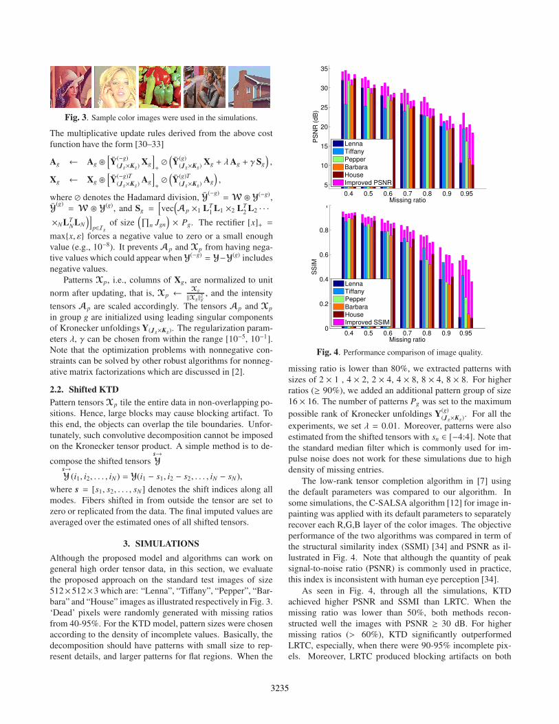
Fig. 3. Sample color images were used in the simulations.

The multiplicative update rules derived from the above cost

function have the form [30–33]

Ag ← Ag ⊛

[

Y(−g)

(Jg×Kg)Xg

]

+⊘(

Y(g)

(Jg×Kg)Xg + λAg + γ Sg

)

,

Xg ← Xg ⊛

[

Y(−g)T

(Jg×Kg)Ag

]

+⊘(

Y(g)T

(Jg×Kg)Ag

)

,

where ⊘ denotes the Hadamard division, Y(−g)= W ⊛ Y

(−g),

Y(g)= W ⊛ Y

(g), and Sg =[

vec(

Ap ×1 LT1

L1 ×2 LT2

L2 · · ·

×NLTN

LN

)]

p∈Ig

of size(

∏

n Jgn

)

× Pg. The rectifier [x]+ =

max{x, ε} forces a negative value to zero or a small enough

value (e.g., 10−8). It prevents Ap and Xp from having nega-

tive values which could appear when Y(−g)= Y−Y

(g) includes

negative values.

Patterns Xp, i.e., columns of Xg, are normalized to unit

norm after updating, that is, Xp ←Xg

‖Xg‖2F

, and the intensity

tensors Ap are scaled accordingly. The tensors Ap and Xp

in group g are initialized using leading singular components

of Kronecker unfoldings Y(Jg×Kg). The regularization param-

eters λ, γ can be chosen from within the range [10−5, 10−1].

Note that the optimization problems with nonnegative con-

straints can be solved by other robust algorithms for nonneg-

ative matrix factorizations which are discussed in [2].

2.2. Shifted KTD

Pattern tensors Xp tile the entire data in non-overlapping po-

sitions. Hence, large blocks may cause blocking artifact. To

this end, the objects can overlap the tile boundaries. Unfor-

tunately, such convolutive decomposition cannot be imposed

on the Kronecker tensor product. A simple method is to de-

compose the shifted tensorss→

Ys→

Y (i1, i2, . . . , iN) = Y(i1 − s1, i2 − s2, . . . , iN − sN),

where s = [s1, s2, . . . , sN] denotes the shift indices along all

modes. Fibers shifted in from outside the tensor are set to

zero or replicated from the data. The final imputed values are

averaged over the estimated ones of all shifted tensors.

3. SIMULATIONS

Although the proposed model and algorithms can work on

general high order tensor data, in this section, we evaluate

the proposed approach on the standard test images of size

512×512×3 which are: “Lenna”, “Tiffany”, “Pepper”, “Bar-

bara” and “House” images as illustrated respectively in Fig. 3.

‘Dead’ pixels were randomly generated with missing ratios

from 40-95%. For the KTD model, pattern sizes were chosen

according to the density of incomplete values. Basically, the

decomposition should have patterns with small size to rep-

resent details, and larger patterns for flat regions. When the

0.4 0.5 0.6 0.7 0.8 0.9 0.955

10

15

20

25

30

35

PS

NR

(dB

)

Missing ratio

LennaTiffanyPepperBarbaraHouseImproved PSNR

0.4 0.5 0.6 0.7 0.8 0.9 0.950

0.2

0.4

0.6

0.8

1

SS

IM

Missing ratio

LennaTiffanyPepperBarbaraHouseImproved SSIM

Fig. 4. Performance comparison of image quality.

missing ratio is lower than 80%, we extracted patterns with

sizes of 2 × 1 , 4 × 2, 2 × 4, 4 × 8, 8 × 4, 8 × 8. For higher

ratios (≥ 90%), we added an additional pattern group of size

16 × 16. The number of patterns Pg was set to the maximum

possible rank of Kronecker unfoldings Y(g)

(Jg×Kg). For all the

experiments, we set λ = 0.01. Moreover, patterns were also

estimated from the shifted tensors with sn ∈ [−4:4]. Note that

the standard median filter which is commonly used for im-

pulse noise does not work for these simulations due to high

density of missing entries.

The low-rank tensor completion algorithm in [7] using

the default parameters was compared to our algorithm. In

some simulations, the C-SALSA algorithm [12] for image in-

painting was applied with its default parameters to separately

recover each R,G,B layer of the color images. The objective

performance of the two algorithms was compared in term of

the structural similarity index (SSMI) [34] and PSNR as il-

lustrated in Fig. 4. Note that although the quantity of peak

signal-to-noise ratio (PSNR) is commonly used in practice,

this index is inconsistent with human eye perception [34].

As seen in Fig. 4, through all the simulations, KTD

achieved higher PSNR and SSMI than LRTC. When the

missing ratio was lower than 50%, both methods recon-

structed well the images with PSNR ≥ 30 dB. For higher

missing ratios (> 60%), KTD significantly outperformed

LRTC, especially, when there were 90-95% incomplete pix-

els. Moreover, LRTC produced blocking artifacts on both

3235

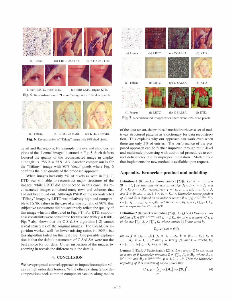
(a) Lenna. (b) LRTC, 25.91 dB. (c) KTD, 28.74 dB.

(d) (left)-LRTC, (right)-KTD. (e) (left)-LRTC, (right)-KTD.

Fig. 5. Reconstruction of “Lenna” image with 70% dead pixels.

(a) Tiffany. (b) LRTC, 22.84 dB. (c) KTD, 27.69 dB.

Fig. 6. Reconstruction of “Tiffany” image with 80% dead pixels.

detail and flat regions, for example, the eye and shoulder re-

gions of the “Lenna” image illustrated in Fig. 5. Such defects

lowered the quality of the reconstructed image in display

although its PSNR = 25.91 dB. Another comparison is for

the “Tiffany” image with 80% ‘dead’ pixels where Fig. 6

confirms the high quality of the proposed approach.

When images had only 5% of pixels as seen in Fig. 7,

KTD was still able to reconstruct major structures of the

images, while LRTC did not succeed in this case. Its re-

constructed images contained many rows and columns that

had not been filled out. Although PSNR of the reconstructed

“Tiffany” image by LRTC was relatively high and compara-

ble to PSNR values in the case of a missing ratio of 90%, this

subjective assessment did not accurately reflect the quality of

this image which is illustrated in Fig. 7(f). For KTD, smooth-

ness constraints were considered for this case with γ = 0.001.

Fig. 7 also shows that the C-SALSA algorithm [12] cannot

reveal structures of the original images. The C-SALSA al-

gorithm worked well for lower missing ratios (≤ 80%), but

this algorithm failed for this test case. One possible explana-

tion is that the default parameters of C-SALSA were not the

best choice for our data. Closer inspection of the images by

zooming in reveals the differences in the details.

4. CONCLUSION

We have proposed a novel approach to impute incomplete val-

ues in high order data tensors. While other existing tensor de-

compositions seek common component vectors along modes

(a) Lenna (b) LRTC. (c) C-SALSA. (d) KTD.

(e) Tiffany (f) LRTC (g) C-SALSA. (h) KTD.

(i) Pepper (j) LRTC (k) C-SALSA. (l) KTD.

Fig. 7. Reconstructed images when there were 95% dead pixels.

of the data tensor, the proposed method retrieves a set of mul-

tiway structured patterns as a dictionary for data reconstruc-

tion. This explains why our approach can work even when

there are only 5% of entries. The performance of the pro-

posed approach can be further improved through multi-level

and multiscale processing with additional procedures to cor-

rect deficiencies due to improper imputation. Matlab code

that implements the new method is available upon request.

Appendix. Kronecker product and unfolding

Definition 1 (Kronecker tensor product [23]). Let A = [a j] and

B = [bk] be two order-N tensors of size J1 × J2 × · · · × JN and

K1 × K2 × · · · × KN , respectively, j = [ j1, j2, . . . , jN ], 1 ≤ jn ≤ Jn

and k = [k1, k2, . . . , kN ], 1 ≤ kn ≤ Kn. A Kronecker tensor product

of A and B is defined as an order-N tensor C = [ci] ∈ RI1×I2×···×IN ,

i = [i1, i2, . . . , iN], In = JnKn such that ci = a j bk, in = kn+ ( jn−1)Kn,

and is expressed as C = A ⊗B.

Definition 2 (Kronecker unfolding [23]). An (J × K) Kronecker un-

folding of C ∈ RI1×I2×···×IN with In = JnKn, for all n, is a matrix C(J×K)

of the size∏N

n=1 Jn ×∏N

n=1 Kn whose entries ( j, k) are given by

C(J×K)( j, k) = C(i),

for all j = [ j1, . . . , jN ], jn = 1, . . . , Jn, k = [k1, . . . , kN ], kn =

1, . . . ,Kn, n = 1, . . . ,N and j = ivec( j, J), and k = ivec(k, K),

i = [i1, . . . , iN], in = kn + ( jn − 1)Kn.

Lemma 1 (Rank-P Factorization [23]). Let a tensor C be expressed

as a sum of P Kronecker products C =∑P

p=1 Ap ⊗Bp, where Ap ∈

RJ1×···×JN and Bp ∈ R

K1×···×KN , p = 1, 2, . . . , P. Then the Kronecker

unfolding of C is a matrix of rank-P, such that

C(J×K) =

P∑

p=1

vec(

Ap

)

vec(

Bp

)T. (4)

3236

5. REFERENCES

[1] R. Bro, Multi-way Analysis in the Food Industry - Models,

Algorithms, and Applications, Ph.D. thesis, University of Am-

sterdam, Holland, 1998.

[2] A. Cichocki, R. Zdunek, A.-H. Phan, and S. Amari, Nonneg-

ative Matrix and Tensor Factorizations: Applications to Ex-

ploratory Multi-way Data Analysis and Blind Source Separa-

tion, Wiley, Chichester, 2009.

[3] T.G. Kolda and B.W. Bader, “Tensor decompositions and ap-

plications,” SIAM Review, vol. 51, no. 3, pp. 455–500, 2009.

[4] M.W. Mahoney, M. Maggioni, and P. Drineas, “Tensor-CUR

decompositions and data applications,” SIAM J. Matrix Anal.

Appl., vol. 30, pp. 957–987, 2008.

[5] G. Tomasi and R. Bro, “PARAFAC and missing values,”

Chemometr. Intell. Lab., vol. 75, no. 2, pp. 163–180, 2005.

[6] S. Gandy, B. Recht, and I. Yamada, “Tensor completion and

low-n-rank tensor recovery via convex optimization,” Inverse

Problems, vol. 27, no. 2, pp. 025010, 2011.

[7] J. Liu, P. Musialski, P. Wonka, and J. Ye, “Tensor completion

for estimating missing values in visual data,” in ICCV, 2009,

pp. 2114–2121.

[8] E. J. Candes and B. Recht, “Exact matrix completion via con-

vex optimization,” Commun. ACM, vol. 55, no. 6, pp. 111–119,

2012.

[9] R. Mazumder, T. Hastie, and R. Tibshirani, “Spectral regular-

ization algorithms for learning large incomplete matrices,” J.

Mach. Learn. Res., vol. 11, pp. 2287–2322, Aug. 2010.

[10] J.-F. Cai, E. J. Candes, and Z. Shen, “A singular value thresh-

olding algorithm for matrix completion,” SIAM J. on Optimiza-

tion, vol. 20, no. 4, pp. 1956–1982, Mar. 2010.

[11] I. Daubechies, M. Defrise, and C. De Mol, “An iterative thresh-

olding algorithm for linear inverse problems with a sparsity

constraint,” Comm. Pure Appl. Math., vol. 57, no. 11, pp.

1413–1457, 2004.

[12] M.V. Alfonso, J.M. Bioucas-Dias, and M.A.T. Figueiredo,

“Fast image recovery using variable splitting and constrained

optimization,” IEEE Trans. Image Process., vol. 19, no. 9, pp.

2345 –2356, sept. 2010.

[13] E. Candes, J. Romberg, and T. Tao, “Stable signal recovery

from incomplete and inaccurate measurements,” Comm. Pure

Appl. Math., vol. 59, no. 8, pp. 1207–1223, 2005.

[14] E. J. Candes, J. Romberg, and T. Tao, “Robust uncertainty

principles: exact signal reconstruction from highly incomplete

frequency information,” IEEE Trans. Inf. Theory, vol. 52, no.

2, pp. 489–509, Feb. 2006.

[15] D.L. Donoho, “Compressed sensing,” IEEE Trans. Inf. Theory,

vol. 52, pp. 1289–1306, Apr. 2006.

[16] R.A. Harshman, “Foundations of the PARAFAC procedure:

Models and conditions for an explanatory multimodal factor

analysis,” UCLA Working Papers in Phonetics, vol. 16, pp.

1–84, 1970.

[17] J.D. Carroll and J.J. Chang, “Analysis of individual differ-

ences in multidimensional scaling via an n-way generalization

of Eckart–Young decomposition,” Psychometrika, vol. 35, no.

3, pp. 283–319, 1970.

[18] L.R. Tucker, “Some mathematical notes on three-mode factor

analysis,” Psychometrika, vol. 31, pp. 279–311, 1966.

[19] E. Acar, D. M. Dunlavy, T. G. Kolda, and M. Mørup, “Scalable

tensor factorizations for incomplete data,” Chemometr. Intell.

Lab., vol. 106, no. 1, pp. 41–56, 2011.

[20] P. Tichavsky, A.-H. Phan, and Z. Koldovsky, “Cramer-Rao-

Induced Bounds for CANDECOMP/PARAFAC tensor decom-

position,” IEEE Trans. Signal Process., accepted for publica-

tion, 2013.

[21] J. Liu, P. Musialski, P. Wonka, and J. Ye, “Tensor comple-

tion for estimating missing values in visual data,” IEEE Trans.

Pattern Anal. Mach. Intell., vol. 99, no. preprints, Jan. 2012.

[22] P.L. Combettes and J.-C. Pesquet, “A Douglas Rachford split-

ting approach to nonsmooth convex variational signal recov-

ery,” Selected Topics in Signal Processing, IEEE Journal of,

vol. 1, no. 4, pp. 564 –574, dec. 2007.

[23] A.-H. Phan, A. Cichocki, P. Tichavsky, D. P. Mandic, and

K. Matsuoka, “On revealing replicating structures in multi-

way data: A novel tensor decomposition approach,” in Latent

Variable Analysis and Signal Separation, vol. 7191 of LNCS,

pp. 297–305. Springer Berlin Heidelberg, 2012.

[24] C. Van Loan and N. Pitsianis, “Approximation with kronecker

products,” in Linear Algebra for Large Scale and Real Time

Applications. 1993, pp. 293–314, Kluwer Publications.

[25] J. G. Nagy and M. E. Kilmer, “Kronecker product approxi-

mation for preconditioning in three-dimensional imaging ap-

plications,” IEEE Trans. Image Process., vol. 15, no. 3, pp.

604–613, 2006.

[26] A. Bouhamidi and K. Jbilou, “A kronecker approximation

with a convex constrained optimization method for blind image

restoration,” Optimization Letters, pp. 1–14, 10.1007/s11590-

011-0370-7.

[27] S. Ragnarsson, Structured Tensor Computations: Blocking,

Symmetries And Kronecker Factorizations, Ph.D. thesis, Cor-

nell University, 2012.

[28] M. Nikolova, “Minimizers of cost-functions involving nons-

mooth data-fidelity terms. application to the processing of out-

liers,” SIAM Journal on Numerical Analysis, vol. 40, no. 3, pp.

965–994, 2002.

[29] A. Cichocki and A.-H. Phan, “Fast local algorithms for large

scale nonnegative matrix and tensor factorizations,” IEICE

Transactions, vol. 92-A, no. 3, pp. 708–721, 2009.

[30] M. E. Daube-Witherspoon and G. Muehllehner, “An itera-

tive image space reconstruction algorthm suitable for volume

ECT,” IEEE Trans. Med. Imag., vol. 5, pp. 61–66, 1986.

[31] H. Lanteri, R. Soummmer, and C. Aime, “Comparison be-

tween ISRA and RLA algorithms: Use of a Wiener filter based

stopping criterion,” Astronomy and Astrophysics Suppleman-

tary Series, vol. 140, pp. 235–246., 1999.

[32] D. D. Lee and H.S. Seung, “Learning of the parts of objects

by non-negative matrix factorization,” Nature, vol. 401, pp.

788–791, 1999.

[33] C. J. Lin, “Projected gradient methods for non-negative matrix

factorization,” Neural Computation, vol. 19, no. 10, pp. 2756–

2779, October 2007.

[34] Z. Wang, A. C. Bovik, H. R. Sheikh, and E. P. Simoncelli,

“Image quality assessment: from error visibility to structural

similarity,” IEEE Trans. Image Process., vol. 13, no. 4, pp.

600–612, 2004.

3237