Optimizing Tensor Decomposition on HPC Systems – Challenges and Approaches

Jee Whan ChoiDept. of Computer and Information Science

University of Oregon

IPDPS HIPS 2019May 20th 2019, Rio de Janeiro, Brazil

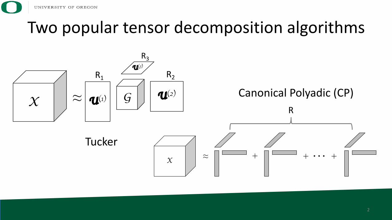
Two popular tensor decomposition algorithms

X ≈ GU(1) U(2)

U(3)

R3

R2R1

X ≈ + ���+ +

Canonical Polyadic (CP)

Tucker

R

2

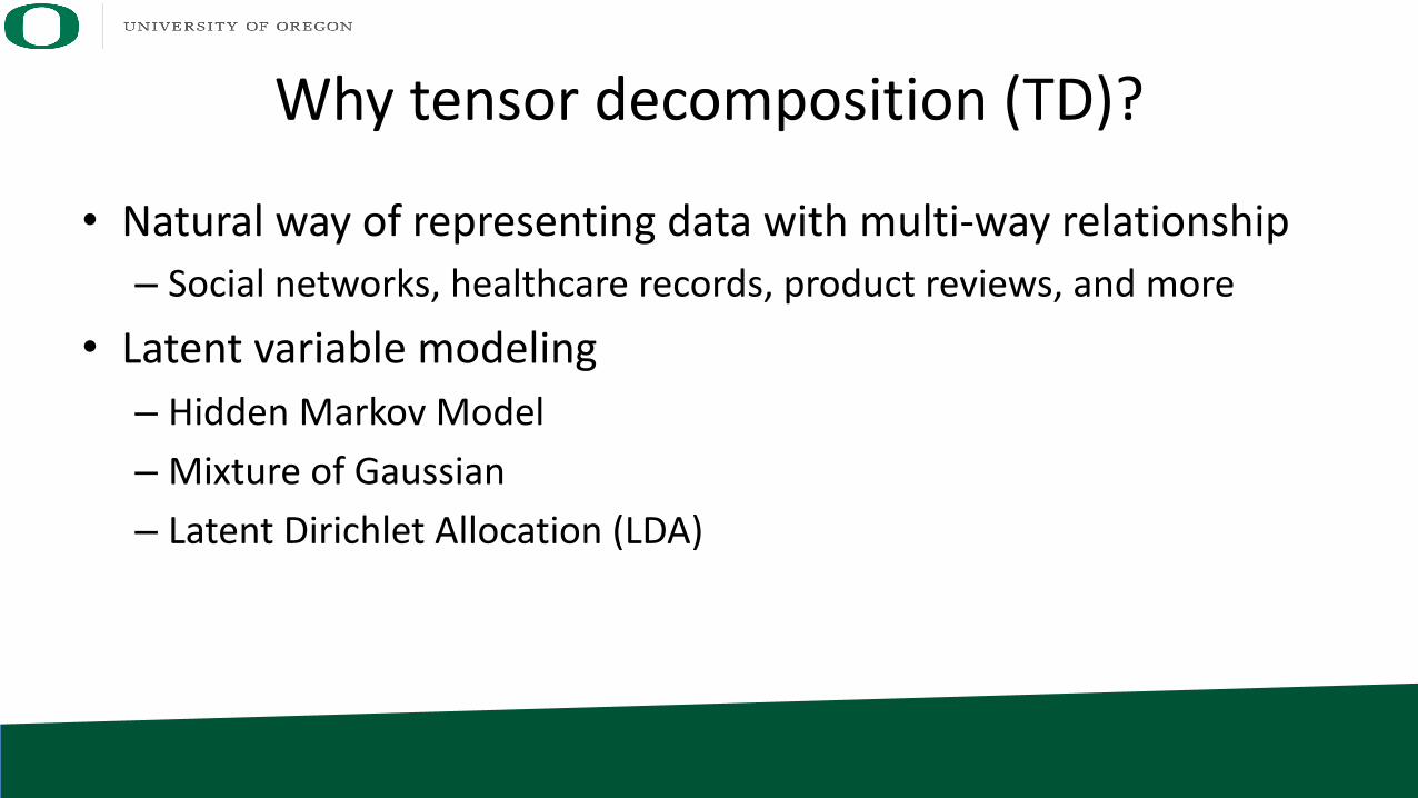
Why tensor decomposition (TD)?

• Natural way of representing data with multi-way relationship– Social networks, healthcare records, product reviews, and more

• Latent variable modeling – Hidden Markov Model– Mixture of Gaussian– Latent Dirichlet Allocation (LDA)

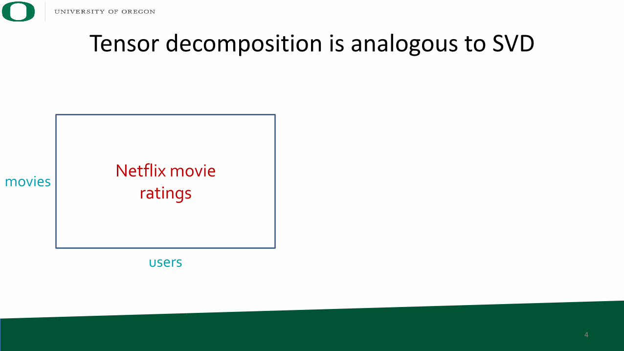
Tensor decomposition is analogous to SVD

4

Netflix movieratings

movies

users

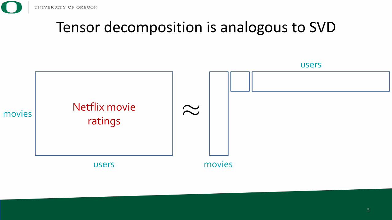
Netflix movieratings

movies

users

⇡

movies

users

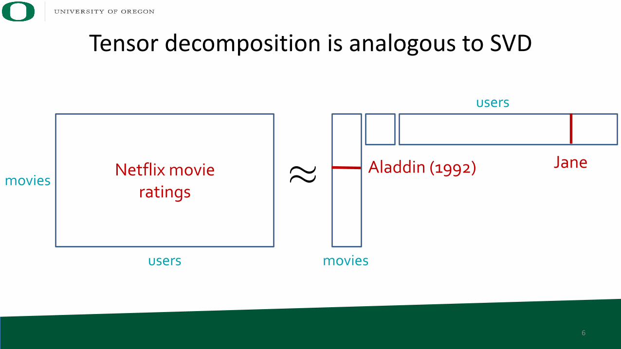
Tensor decomposition is analogous to SVD

5

6

Netflix movieratings

movies

users

⇡

movies

users

Aladdin (1992) Jane

Tensor decomposition is analogous to SVD

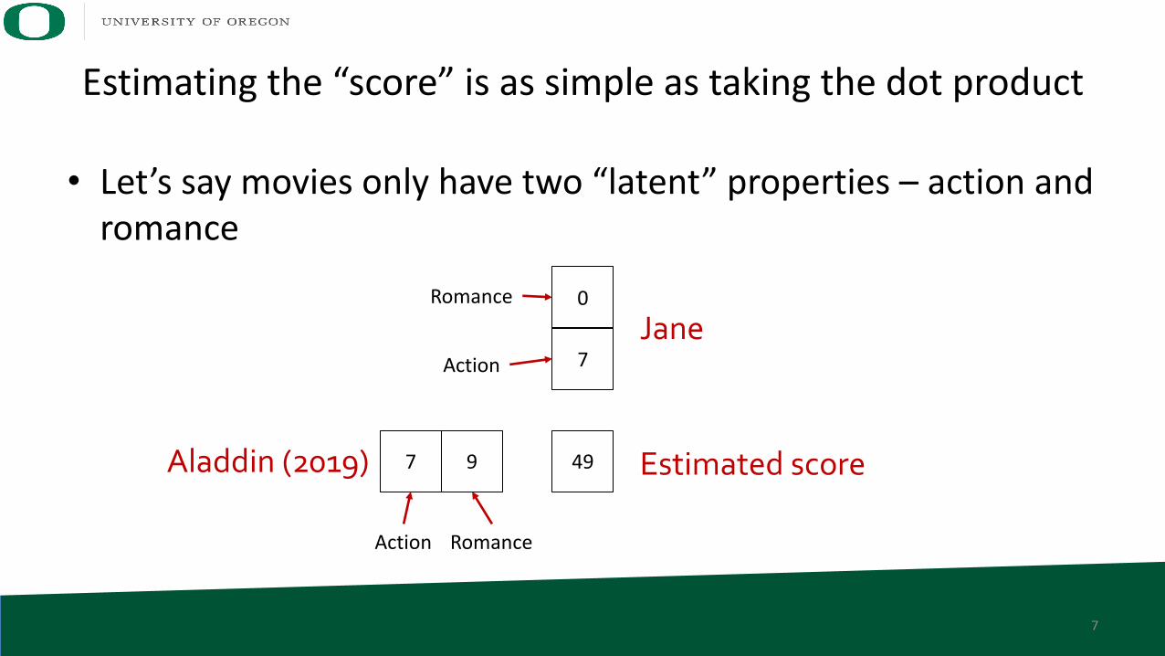
Estimating the “score” is as simple as taking the dot product

• Let’s say movies only have two “latent” properties – action and romance

7 9Aladdin (2019)

7

0

Action Romance

JaneAction

Romance

49 Estimated score

7

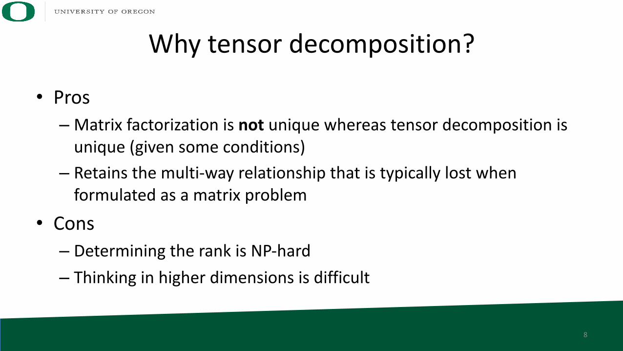
Why tensor decomposition?

• Pros– Matrix factorization is not unique whereas tensor decomposition is

unique (given some conditions)– Retains the multi-way relationship that is typically lost when

formulated as a matrix problem

• Cons– Determining the rank is NP-hard– Thinking in higher dimensions is difficult

8

Applications of tensor decomposition

• Signal processing– Signal separation, code division

• Data analysis– Phenotyping (electronic health record), network analysis, data

compression• Machine learning– Latent variable model (natural language processing, topic modeling,

recommender systems, etc.)– Neural network compression

9

My prior work has covered both dense and sparse data for CP and Tucker

• Sparse tensors– Blocking sparse tensors on shared- and distributed-memory systems

for CPD– Workload balancing for sparse Tucker on distributed-memory

systems

• Dense tensors– Using GPUs to accelerate dense Tucker algorithms– Workload balancing for dense Tucker on distributed-memory systems

10

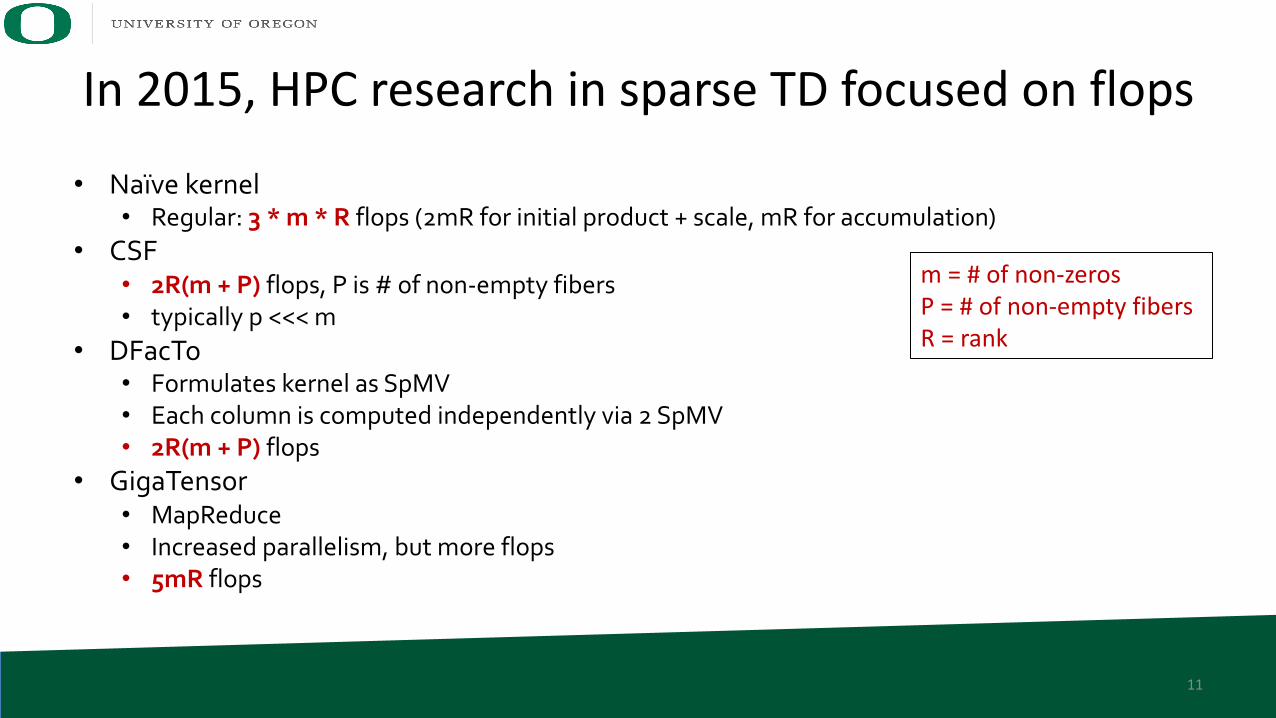
In 2015, HPC research in sparse TD focused on flops

• Naïve kernel• Regular: 3 * m * R flops (2mR for initial product + scale, mR for accumulation)

• CSF• 2R(m + P) flops, P is # of non-empty fibers• typically p <<< m

• DFacTo• Formulates kernel as SpMV• Each column is computed independently via 2 SpMV• 2R(m + P) flops

• GigaTensor• MapReduce• Increased parallelism, but more flops• 5mR flops

m = # of non-zerosP = # of non-empty fibersR = rank

11

Does this make sense for sparse data?

• Sparse computations are generally memory bandwidth-bound• So, why was CSF, DFacto giving better performance?

12

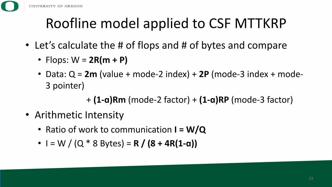
• Let’s calculate the # of flops and # of bytes and compare• Flops: W = 2R(m + P)• Data: Q = 2m (value + mode-2 index) + 2P (mode-3 index + mode-

3 pointer)+ (1-ɑ)Rm (mode-2 factor) + (1-ɑ)RP (mode-3 factor)

• Arithmetic Intensity • Ratio of work to communication I = W/Q• I = W / (Q * 8 Bytes) = R / (8 + 4R(1-ɑ))

13

Roofline model applied to CSF MTTKRP

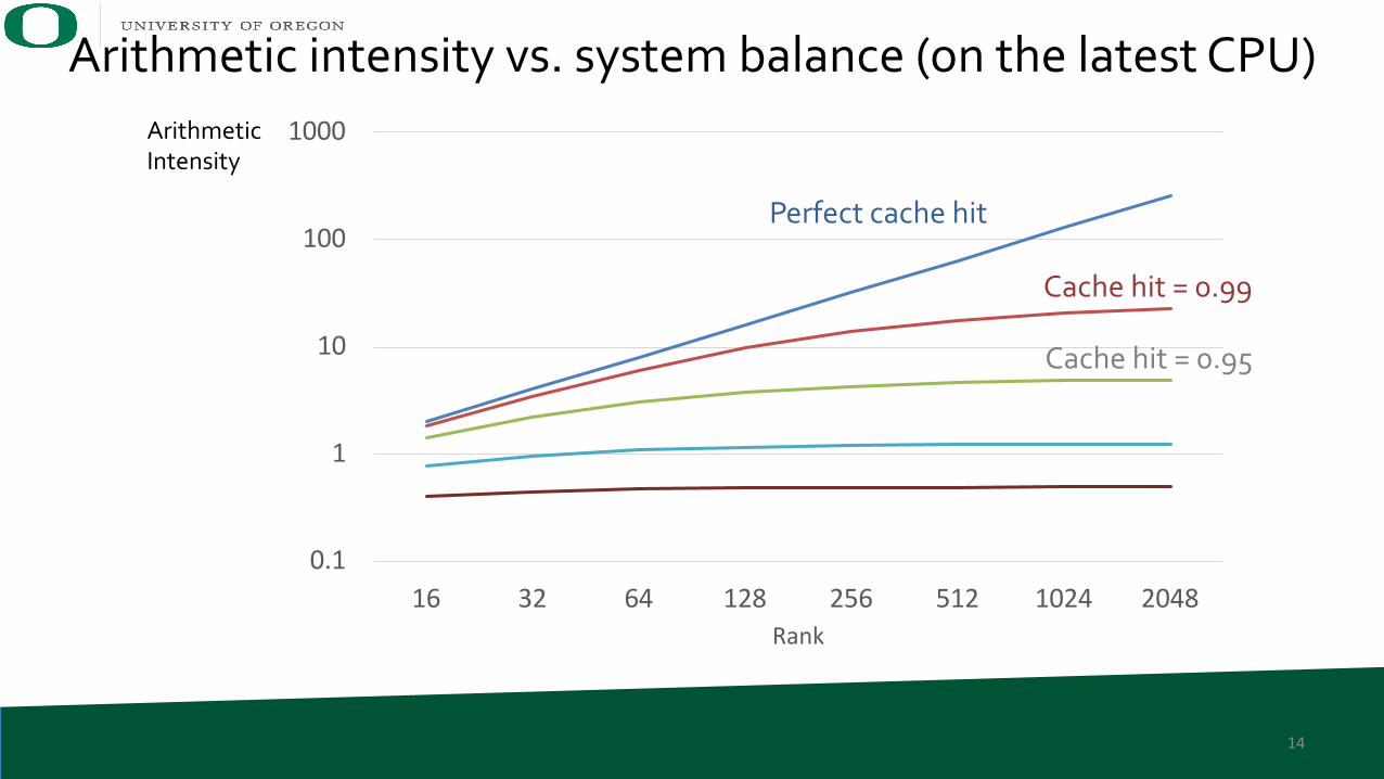
0.1

1

10

100

1000

16 32 64 128 256 512 1024 2048Rank

Perfect cache hit

Cache hit = 0.99

Cache hit = 0.95

Arithmetic intensity vs. system balance (on the latest CPU)Arithmetic Intensity

14

15

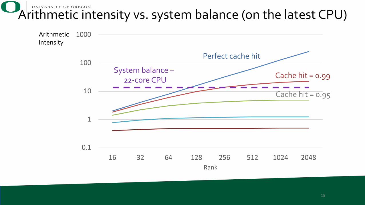
0.1

1

10

100

1000

16 32 64 128 256 512 1024 2048Rank

Perfect cache hit

Cache hit = 0.99

Cache hit = 0.95

Arithmetic intensity vs. system balance (on the latest CPU)Arithmetic Intensity

System balance –22-core CPU

• Pressure point analysis– Probe potential bottlenecks by creating and eliminating

instructions/data access– If we suspect that # of registers is the bottleneck, try

increasing/decreasing their usage to see if the exec. time changes.– Source code & assembly instrumentation – e.g., inline assembly to

prevent dead code elimination (DCE)

16Kenneth Czechowski, Performance Analysis Using the Pressure Point Analysis, PhD dissertation

Pressure point analysis (PPA) reveals the bottlenecks

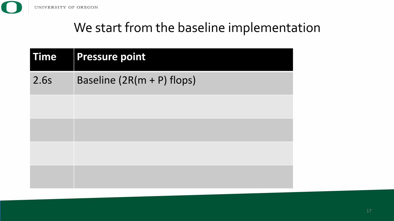
17

We start from the baseline implementation

Time Pressure point

2.6s Baseline (2R(m + P) flops)

18

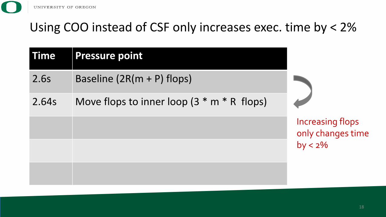
Time Pressure point

2.6s Baseline (2R(m + P) flops)

2.64s Move flops to inner loop (3 * m * R flops)

Increasing flopsonly changes timeby < 2%

Using COO instead of CSF only increases exec. time by < 2%

19

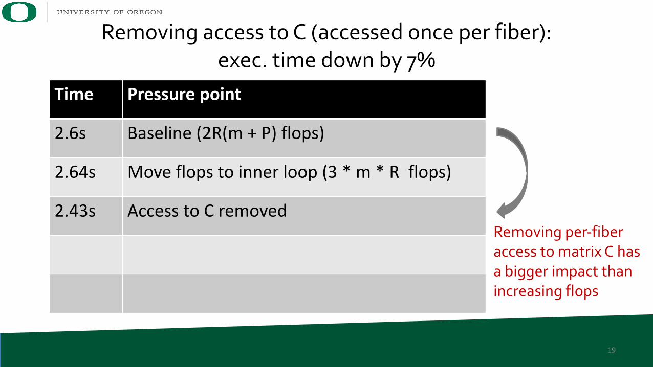
Time Pressure point

2.6s Baseline (2R(m + P) flops)

2.64s Move flops to inner loop (3 * m * R flops)

2.43s Access to C removed Removing per-fiber access to matrix C has a bigger impact than increasing flops

Removing access to C (accessed once per fiber):exec. time down by 7%

20

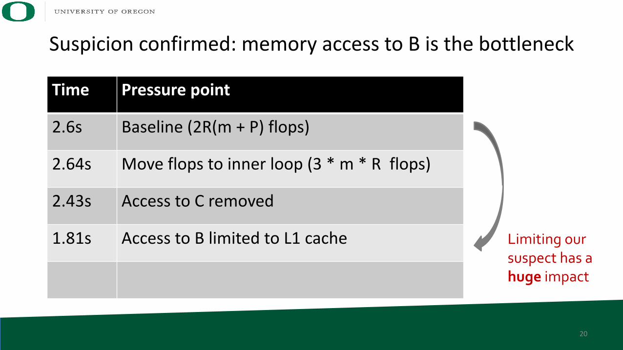
Time Pressure point

2.6s Baseline (2R(m + P) flops)

2.64s Move flops to inner loop (3 * m * R flops)

2.43s Access to C removed

1.81s Access to B limited to L1 cache Limiting our suspect has a huge impact

Suspicion confirmed: memory access to B is the bottleneck

21

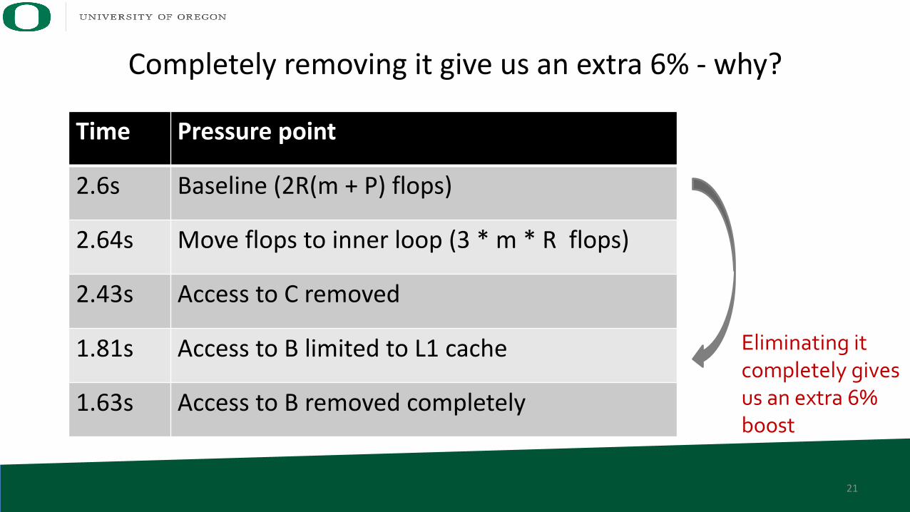
Time Pressure point

2.6s Baseline (2R(m + P) flops)

2.64s Move flops to inner loop (3 * m * R flops)

2.43s Access to C removed

1.81s Access to B limited to L1 cache

1.63s Access to B removed completely

Eliminating itcompletely givesus an extra 6%boost

Completely removing it give us an extra 6% - why?

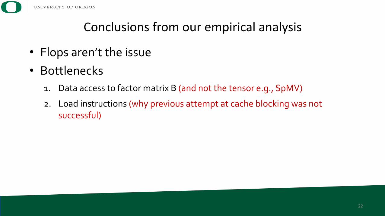
• Flops aren’t the issue• Bottlenecks

1. Data access to factor matrix B (and not the tensor e.g., SpMV)

2. Load instructions (why previous attempt at cache blocking was not successful)

22

Conclusions from our empirical analysis

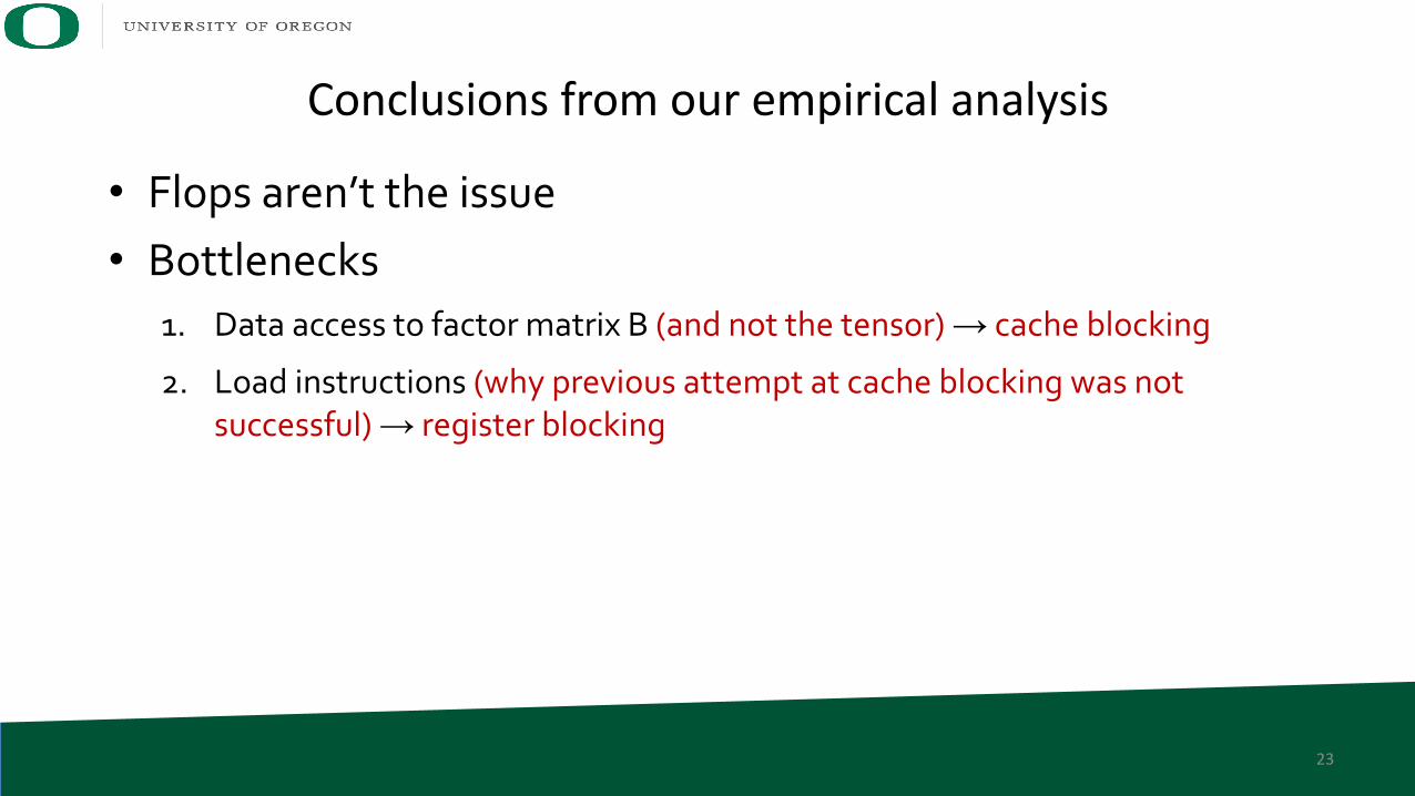
• Flops aren’t the issue• Bottlenecks

1. Data access to factor matrix B (and not the tensor) → cache blocking

2. Load instructions (why previous attempt at cache blocking was not successful) → register blocking

23

Conclusions from our empirical analysis

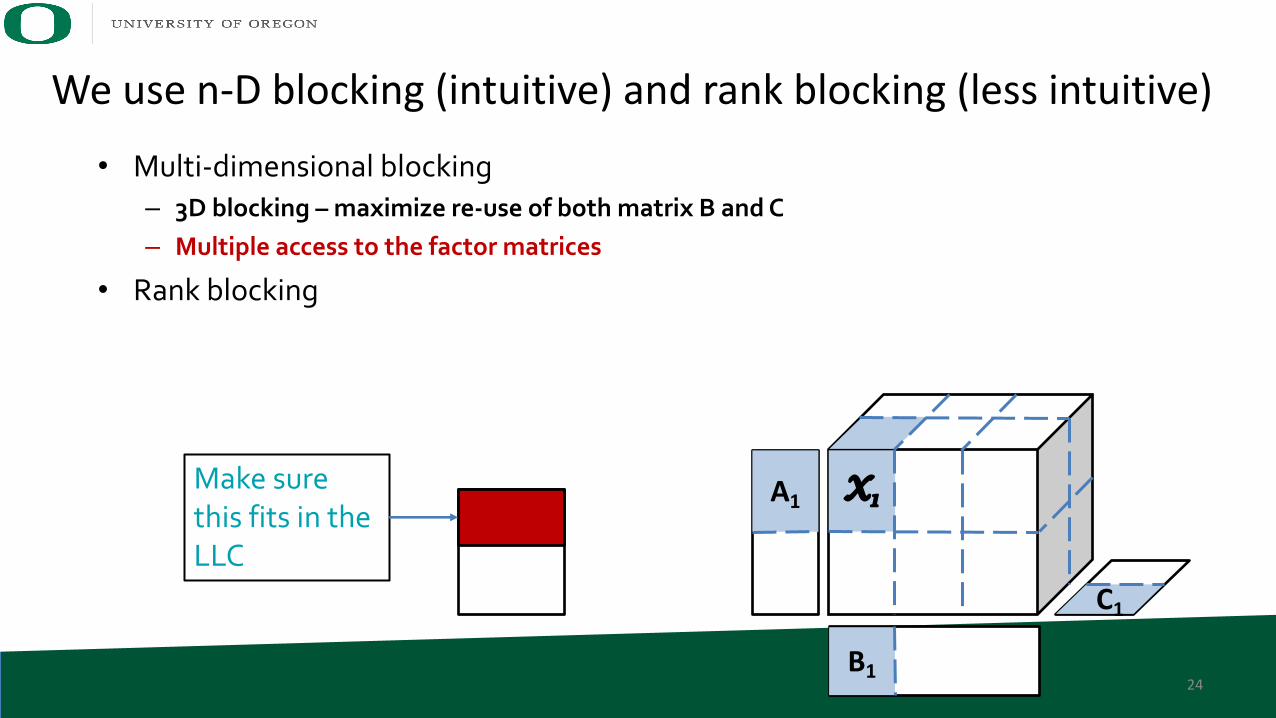
• Multi-dimensional blocking– 3D blocking – maximize re-use of both matrix B and C– Multiple access to the factor matrices

• Rank blocking

24

X1A1

B1

C1

We use n-D blocking (intuitive) and rank blocking (less intuitive)

Make surethis fits in the LLC

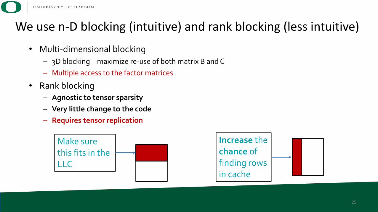
• Multi-dimensional blocking– 3D blocking – maximize re-use of both matrix B and C– Multiple access to the factor matrices

• Rank blocking– Agnostic to tensor sparsity– Very little change to the code– Requires tensor replication

25

Make surethis fits in the LLC

We use n-D blocking (intuitive) and rank blocking (less intuitive)

Increase thechance offinding rowsin cache

26

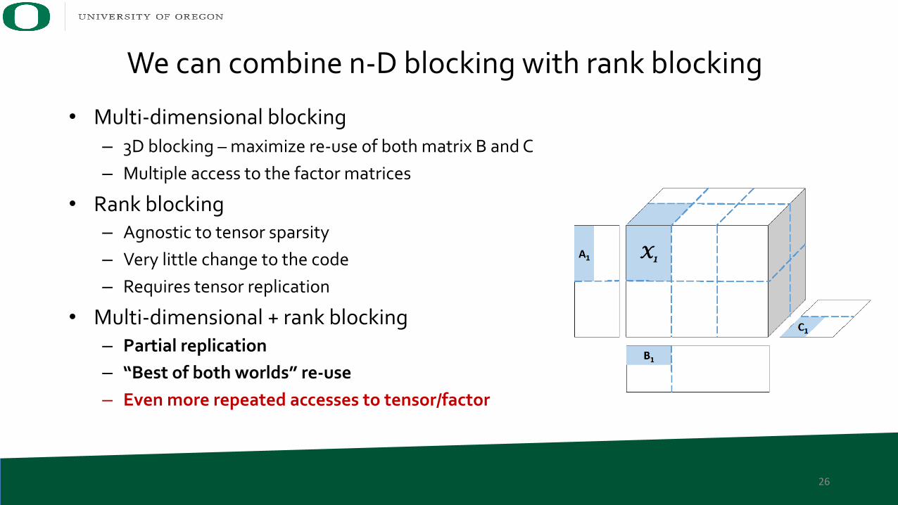
• Multi-dimensional blocking– 3D blocking – maximize re-use of both matrix B and C– Multiple access to the factor matrices

• Rank blocking– Agnostic to tensor sparsity– Very little change to the code– Requires tensor replication

• Multi-dimensional + rank blocking– Partial replication– “Best of both worlds” re-use– Even more repeated accesses to tensor/factor

We can combine n-D blocking with rank blocking

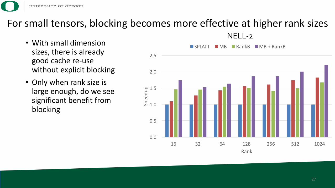
For small tensors, blocking becomes more effective at higher rank sizes

27

0.0

0.5

1.0

1.5

2.0

2.5

16 32 64 128 256 512 1024Speedu

pRank

SPLATT MB RankB MB+RankB• With small dimension sizes, there is already good cache re-use without explicit blocking• Only when rank size is

large enough, do we see significant benefit from blocking

NELL-2

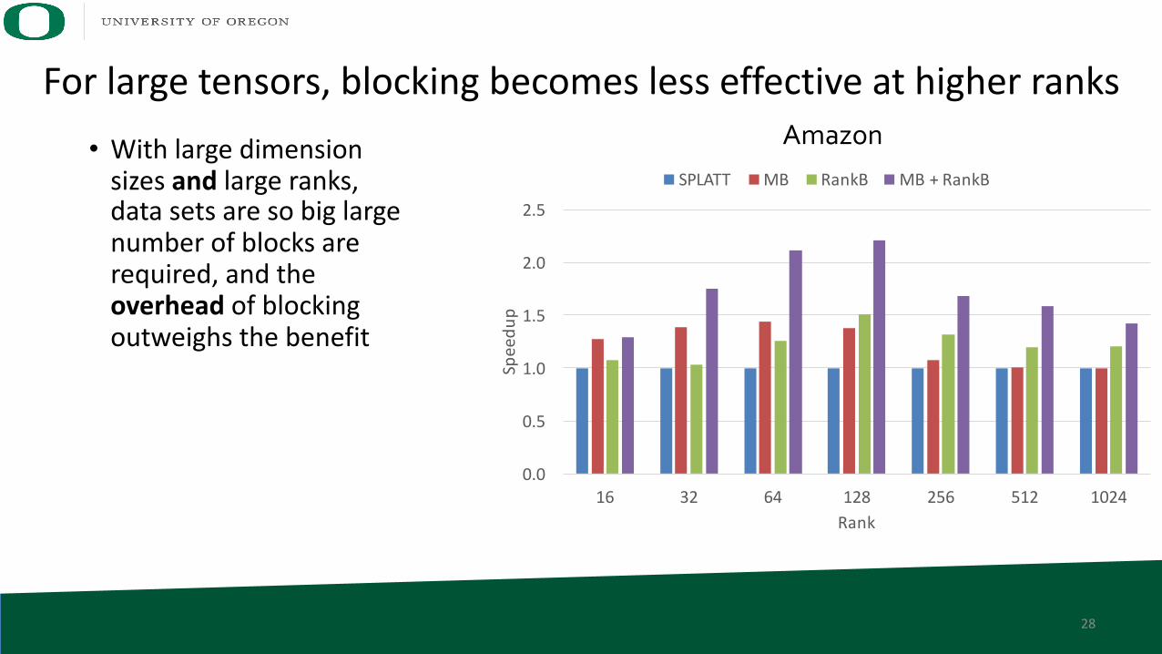
For large tensors, blocking becomes less effective at higher ranks

28

• With large dimension sizes and large ranks, data sets are so big large number of blocks are required, and the overhead of blocking outweighs the benefit

Amazon

0.0

0.5

1.0

1.5

2.0

2.5

16 32 64 128 256 512 1024Speedu

pRank

SPLATT MB RankB MB+RankB

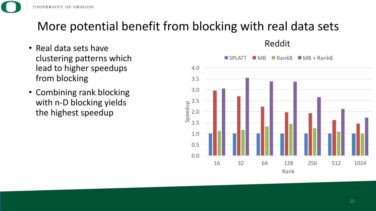
More potential benefit from blocking with real data sets

29

• Real data sets have clustering patterns which lead to higher speedups from blocking• Combining rank blocking

with n-D blocking yields the highest speedup

Reddit

0.0

0.5

1.0

1.5

2.0

2.5

3.0

3.5

4.0

16 32 64 128 256 512 1024

Speedu

p

Rank

SPLATT MB RankB MB+RankB

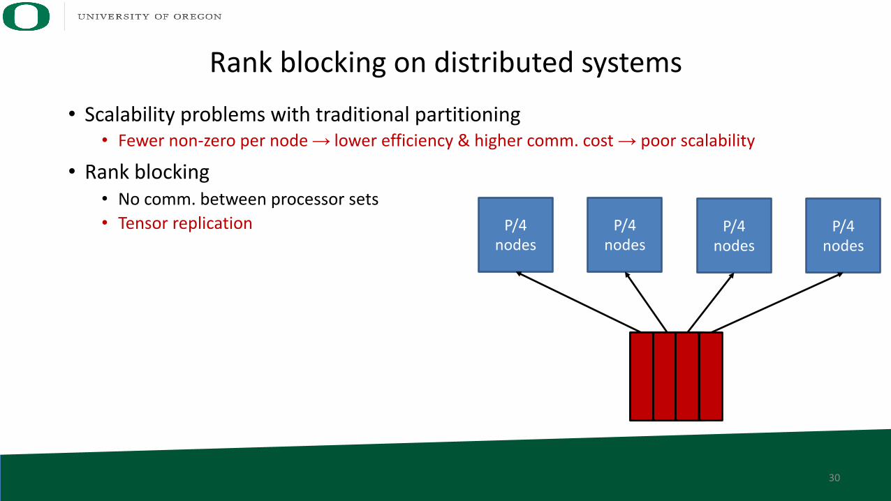
Rank blocking on distributed systems

30

• Scalability problems with traditional partitioning• Fewer non-zero per node→ lower efficiency & higher comm. cost → poor scalability

• Rank blocking• No comm. between processor sets• Tensor replication P/4

nodesP/4

nodesP/4

nodesP/4

nodes

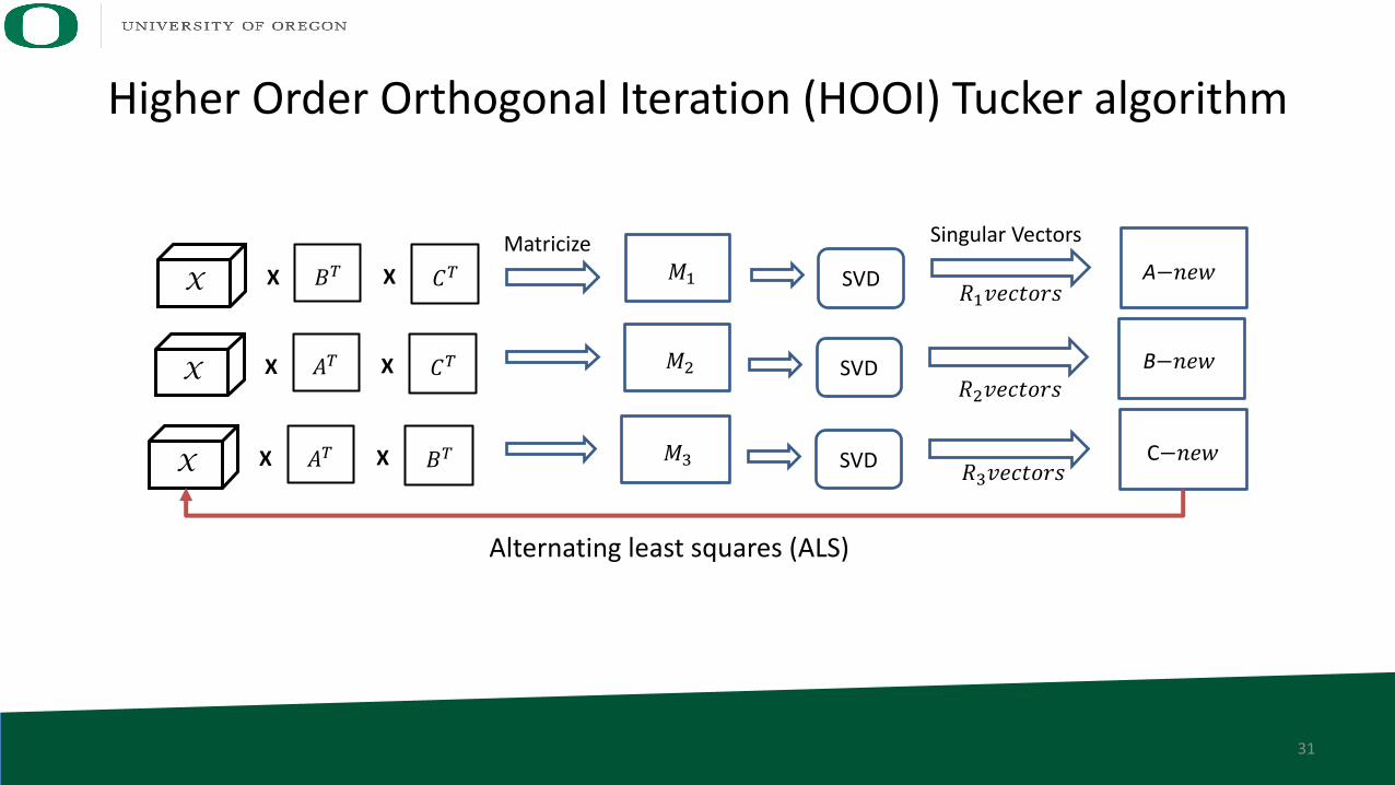
Higher Order Orthogonal Iteration (HOOI) Tucker algorithm

X 𝐵" 𝐶"X X SVD𝑀%

X 𝐴" 𝐶"X X SVD B−𝑛𝑒𝑤𝑀+

X 𝐴" 𝐵"X X SVD C−𝑛𝑒𝑤𝑀,

Matricize Singular Vectors

𝑅%𝑣𝑒𝑐𝑡𝑜𝑟𝑠

𝑅+𝑣𝑒𝑐𝑡𝑜𝑟𝑠

𝑅,𝑣𝑒𝑐𝑡𝑜𝑟𝑠

A−𝑛𝑒𝑤

Alternating least squares (ALS)

31

Sparse HOOI – key kernels

• TTM• Computation only - all schemes have same computational load (i.e., FLOPs)• Load balance

• SVD• Both computation and communication• Both computational load and communication volume are determined by load balance

• Factor Matrix Transfer (FMT)• Communication only• At the end of each HOOI invocation, factor matrix rows need to be communicated among

processors for the next invocation• Communication volume

32

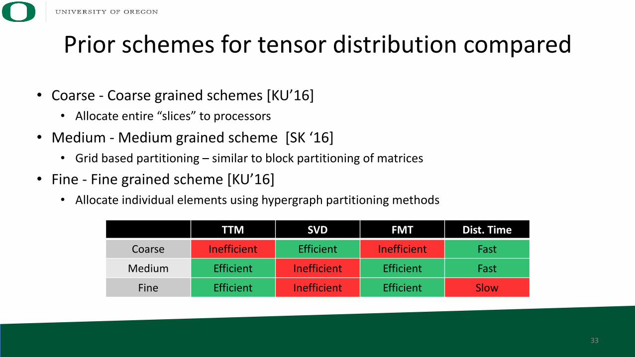
Prior schemes for tensor distribution compared

• Coarse - Coarse grained schemes [KU’16]• Allocate entire “slices” to processors

• Medium - Medium grained scheme [SK ‘16]• Grid based partitioning – similar to block partitioning of matrices

• Fine - Fine grained scheme [KU’16]• Allocate individual elements using hypergraph partitioning methods

TTM SVD FMT Dist. Time

Coarse Inefficient Efficient Inefficient Fast

Medium Efficient Inefficient Efficient Fast

Fine Efficient Inefficient Efficient Slow

33

Our scheme – lite distribution – achieves better workload distribution

• Lite– Near optimal on TTM and SVD (both computation and communication)– Lightweight (i.e., fast distribution time)– Not optimal on FMT (but this is cheap)– Performance gain up to 3×

34

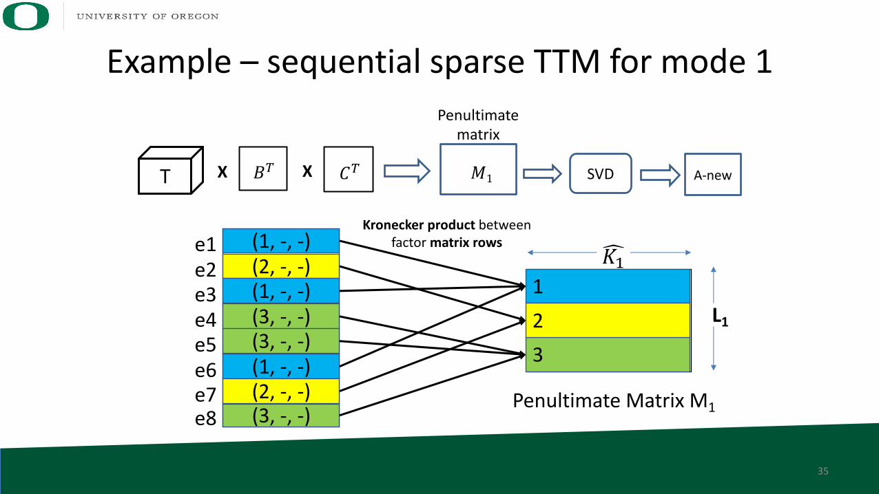
Example – sequential sparse TTM for mode 1

T 𝐵" 𝐶"X X SVD A-new𝑀1

Penultimatematrix

Kronecker product between factor matrix rows

3

12

(1, -, -)e1(2, -, -)e2(1, -, -)e3(3, -, -)e4(3, -, -)e5(1, -, -)e6(2, -, -)e7(3, -, -)e8

Penultimate Matrix M1

6𝐾%

L1

35

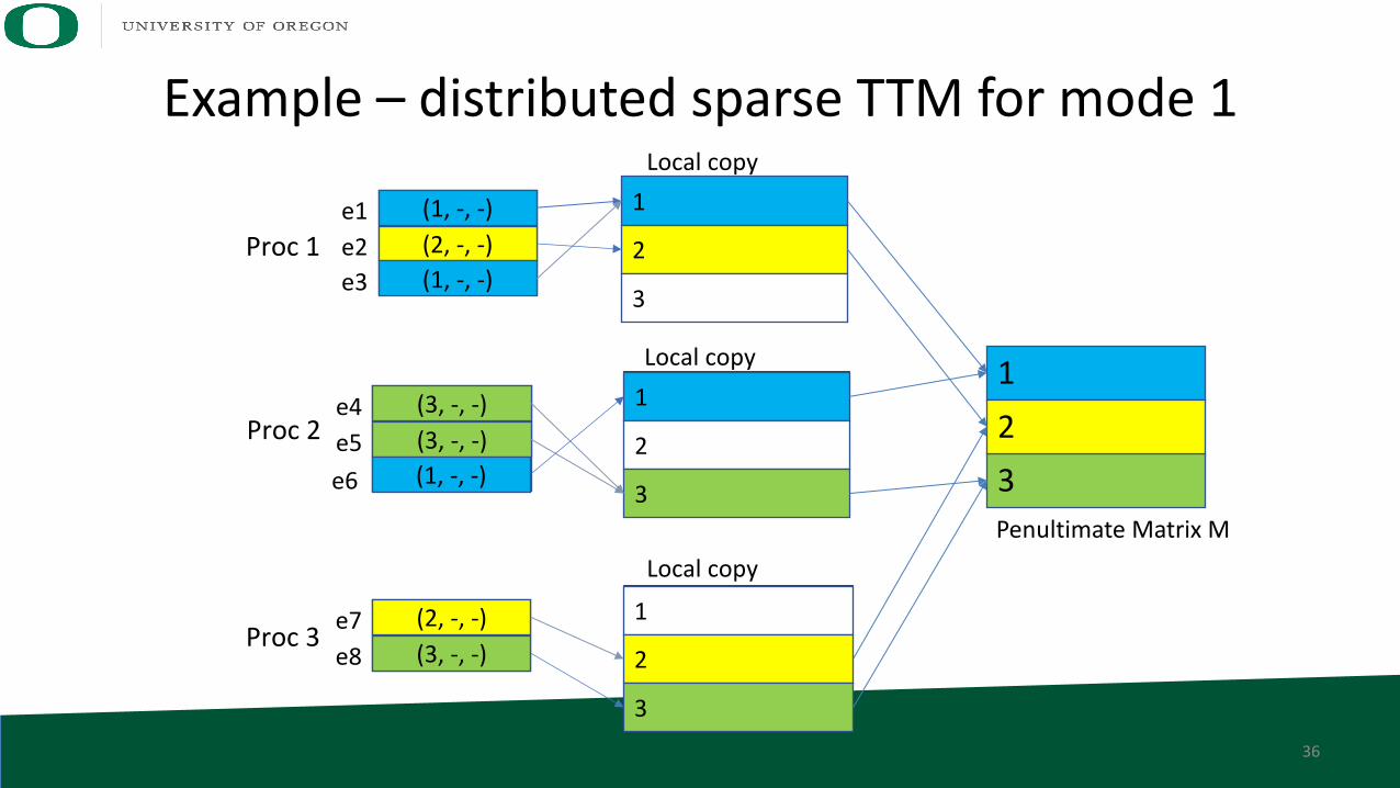
Example – distributed sparse TTM for mode 1

Local copy

1

2

3

(1, -, -)e1(2, -, -)e2(1, -, -)e3

1

2

3

(3, -, -)e4(3, -, -)e5(1, -, -)e6

1

2

3

(2, -, -)e7(3, -, -)e8

Proc 1

Proc 2

Proc 3

Local copy

Local copy

3

12

Penultimate Matrix M

36

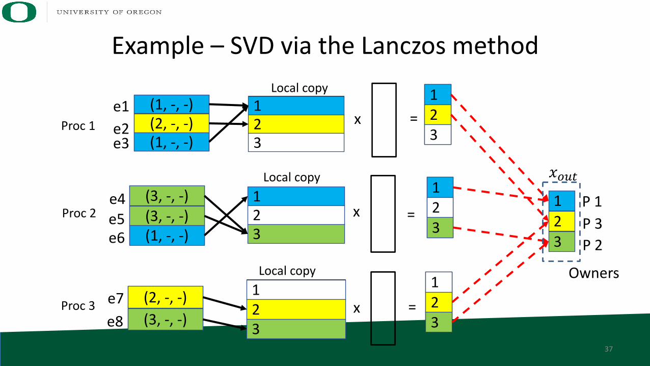
Example – SVD via the Lanczos method

Local copy

123

e1e2

(1, -, -)(2, -, -)(1, -, -)e3

123

e4e5

(3, -, -)(3, -, -)(1, -, -)e6

123

e7 (2, -, -)(3, -, -)e8

Proc 1

Proc 2

Proc 3

Local copy

Local copy 123

123

123

=

=

=

123

𝑥9:;P 1P 3P 2

x

x

x

Owners

37

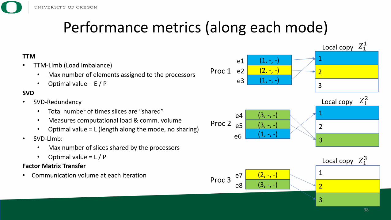
TTM• TTM-LImb (Load Imbalance)

• Max number of elements assigned to the processors• Optimal value – E / P

SVD• SVD-Redundancy

• Total number of times slices are “shared”• Measures computational load & comm. volume• Optimal value = L (length along the mode, no sharing)

• SVD-LImb: • Max number of slices shared by the processors• Optimal value = L / P

Factor Matrix Transfer• Communication volume at each iteration

Performance metrics (along each mode)

Local copy

1

2

3

(1, -, -)e1(2, -, -)e2(1, -, -)e3

1

2

3

(3, -, -)e4(3, -, -)e5(1, -, -)e6

1

2

3

(2, -, -)e7(3, -, -)e8

Proc 1

Proc 2

Proc 3

𝑍%%

𝑍%+

𝑍%,Local copy

Local copy

38

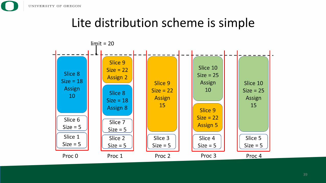
Lite distribution scheme is simple

39

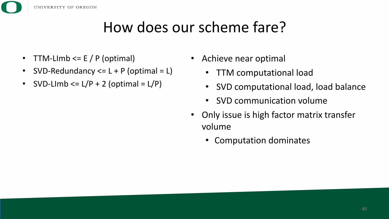
How does our scheme fare?

• TTM-LImb <= E / P (optimal)• SVD-Redundancy <= L + P (optimal = L)• SVD-LImb <= L/P + 2 (optimal = L/P)

• Achieve near optimal • TTM computational load• SVD computational load, load balance • SVD communication volume

• Only issue is high factor matrix transfer volume• Computation dominates

40

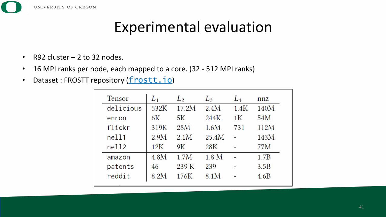
Experimental evaluation

• R92 cluster – 2 to 32 nodes. • 16 MPI ranks per node, each mapped to a core. (32 - 512 MPI ranks)• Dataset : FROSTT repository (frostt.io)

41

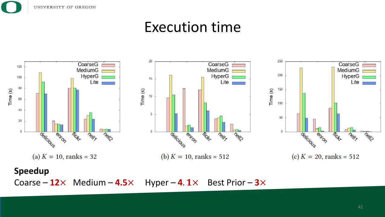
Execution time

SpeedupCoarse – 12× Medium – 4.5× Hyper – 4. 𝟏× Best Prior – 3×

42

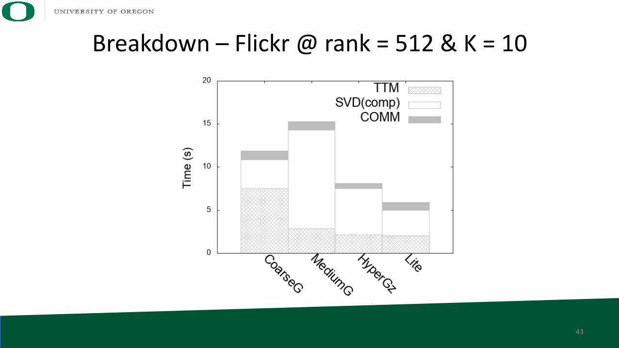
Breakdown – Flickr @ rank = 512 & K = 10

43

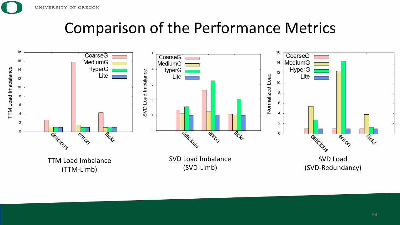
Comparison of the Performance Metrics

TTM Load Imbalance(TTM-Limb)

SVD Load(SVD-Redundancy)

SVD Load Imbalance(SVD-Limb)

44

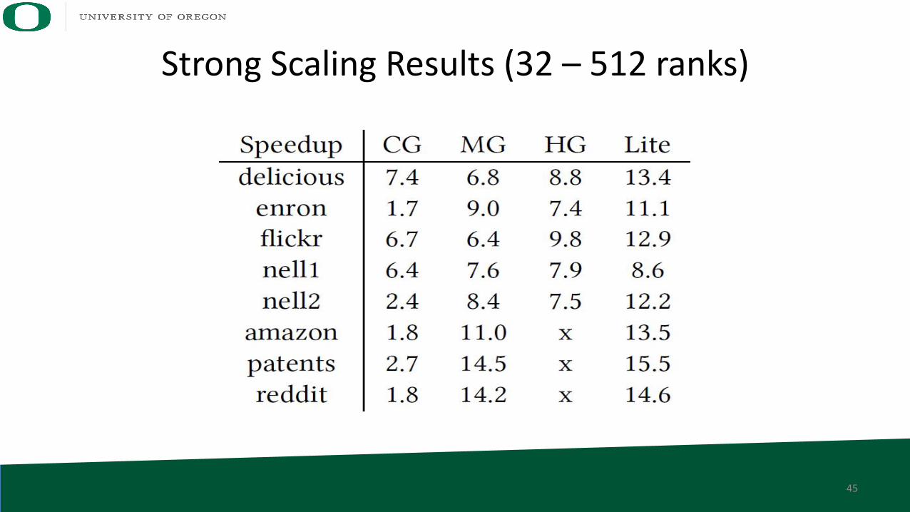
Strong Scaling Results (32 – 512 ranks)

45

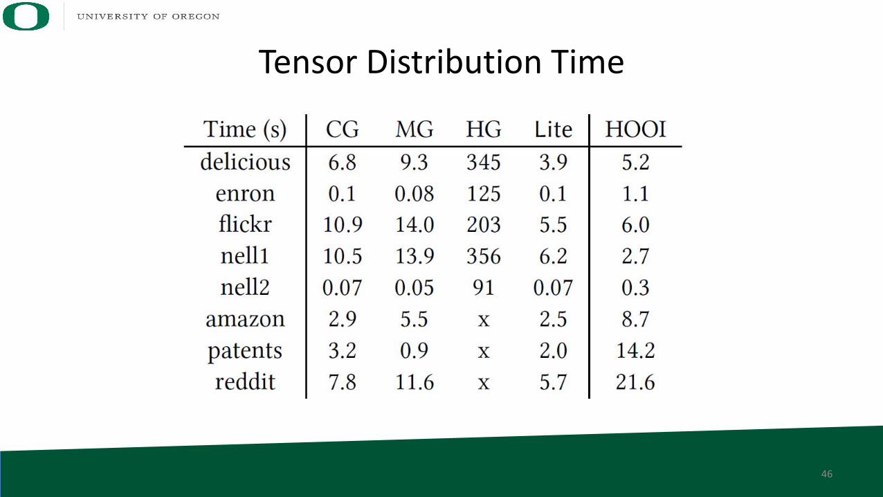
Tensor Distribution Time

46

Challenges and possible solutions

• Data locality (both shared and distributed) is important in performance of TD algorithms– However, due to the diversity of the kernels, there is no single solution– High dimensionality makes everything more difficult

• Ideally– Finding the right programming model/abstraction for capturing data

distribution (shared and distributed) and its impact on performance– Domain-specific language/compiler to overcome tensor-specific

bottlenecks– Optimized libraries

47

Future work

• Future work– Efficient data structures for sparse tensors– Modeling the sparsity– Near-memory processing architectures for tensor computation– Energy efficiency (on mobile devices)

48

Reference• [1] Jee W. Choi, Xing Liu, Shaden Smith, Tyler Simon, Blocking Optimization Techniques for Sparse

Tensor Computation. 32nd IEEE International Parallel and Distributed Processing Symposium (IPDPS’18).

• [2] Venkatesan T. Chakaravarthy, Jee W. Choi, Douglas J. Joseph, Prakash Murali, Yogish Sabharwal, S. Shivmaran, Dheeraj Sreedhar, On Optimizing Distributed Tucker Decomposition for Sparse Tensors. The 32nd ACM International Conference on Supercomputing (ICS’18).

• [3] Jee W. Choi, Xing Liu, Venkatesan T. Chakaravarthy, High-performance Dense Tucker Decomposition on GPU Clusters. The International Conference for High Performance Computing, Networking, Storage, and Analysis (SC’18).

• [4] Venkatesan T. Chakaravarthy, Jee W. Choi, Xing Liu, Douglas J. Joseph, Prakash Murali, Yogish Sabharwal, Dheeraj Sreedhar, On Optimizing Distributed Tucker Decomposition for Dense Tensors. 31st IEEE International Parallel and Distributed Processing Symposium (IPDPS’17).