Full waveform inversion of a 3-D source inside an …glaser.berkeley.edu/glaserdrupal/pdf/JSV 2005.pdfJOURNAL OF SOUND AND VIBRATION Journal of Sound and Vibration 285 (2005) 835–857

ARTICLE IN PRESS

JOURNAL OFSOUND ANDVIBRATION

Journal of Sound and Vibration 285 (2005) 835–857

0022-460X/$ -

doi:10.1016/j.

�Correspon

Berkeley, Ber

E-mail add

www.elsevier.com/locate/jsvi

Full waveform inversion of a 3-D sourceinside an artificial rock

Albert C. Toa,b, Steven D. Glasera,b,�

aCenter for Information Technology Research in the Interest of Society, University of Berkeley, Berkeley, CA, USAb281 Hearst Memorial Mining Building, Berkeley, CA 94120-1761, USA

Received 3 March 2004; received in revised form 18 August 2004; accepted 31 August 2004

Available online 18 December 2004

Abstract

A full waveform inversion of the kinematics of a 3-D source inside an artificial rock plate is presented.The source is provided by a piezoelectric disc embedded inside a gypsum plate, excited by an arbitraryelectrical signal. Elastic waves emitted from the source propagated through the plate and were recorded byan array of wide-band high-fidelity microseismic displacement sensors. These microseismic data are theninverted by deconvolving the recorded signals with the theoretical Green’s functions to obtain thekinematics of the source modeled by force couples. The force time functions thus inverted are justifiedqualitatively by the known mechanical behavior and compared quantitatively to simplified electro-acousticequations. For the first time, the combined use of a wide-band high-fidelity sensor, Green’s functionsincorporating Q damping, effective point source theory, and linear deconvolution yield physically justifiedtime functions of the source kinematics.r 2004 Elsevier Ltd. All rights reserved.

1. Introduction

Determination of the kinematics of crack growth is of great importance in engineering andscience. The kinematics of a source within a solid can in theory be estimated by inverting recordedmicroseismic (MS) signals generated by the source. In the present paper, a full waveform inversion

see front matter r 2004 Elsevier Ltd. All rights reserved.

jsv.2004.09.001

ding author. Center for Information Technology Research in the Interest of Society, University of

keley, CA 94122, USA. Tel.: +1 510 642 1264; fax: +1510 642 7476.

ress: [email protected] (S.D. Glaser).

www.elsevier.com/locate/jsvi

ARTICLE IN PRESS

A.C. To, S.D. Glaser / Journal of Sound and Vibration 285 (2005) 835–857836

of the kinematics of a 3-D source inside an artificial rock plate is presented. The 3-D source is apiezoelectric disc that expands (or contracts) in the axial direction and contracts (or expands) inthe radial direction due to the input of an arbitrary electric signal.

Inversion methods can be generally divided into three categories: (1) inversion by use of onlythe initial p-wave amplitude, (2) full waveform inversion by empirical Green’s function, and (3)full waveform inversion by theoretical Green’s function. In the first category, only the amplitudeof the first p-wave pulse is used to determine the type of crack and the size of the source [1–3]. Thismethod will lead to an answer very quickly and does not require the use of Green’s functions, butit does not give the complete behavior of the crack as a function of time.

In the second category, the MS signals are inverted from an empirical Green’s function toobtain time function of the kinematics [4–6]. The resulting source time function is very accuratebecause the empirical Green’s function accounts for the receiver transfer function and anelasticitywhich arises from crystal defects, grain-boundary processes, and viscoelasticity, which are difficultto account for individually when calculating a theoretical Green’s function. However, obtainingthe empirical Green’s function is practically impossible inside a solid without disturbing the solid(except when the source is a monopole on the surface of a solid).

In the third category, the MS signals are inverted from the calculated theoretical Green’sfunctions to obtain the kinematics of the source [7]. The most direct inversion method is by directlinear deconvolution of the MS data from the calculated Green’s functions [8,9]. The lineardeconvolution method can be used to invert for sources of any nature and location, but thesuccess of this method hinges on (1) how close the solid model used to calculate the Green’sfunction is to the actual physical properties of the solid, and (2) the estimation of the transferfunction of the transducer. Errors in the Green’s function and the transducer transfer function areprojected onto the resulting source time functions and render them physically unjustified. Veryfew works to date have applied this method successfully to MS data. Kim and Sachse [10,11]presented a full waveform inversion of indentation cracks and thermal cracks in glass,respectively. In Enoki and Kishi [12], recorded signals due to cracks were inverted to give thesource time function for a fracture toughness testing in steel. Shah and Labuz [13] studiedthe damage mechanisms in stressed rock by performing full waveform inversion. In these works,the material is assumed to be elastic, isotropic, and homogeneous, while the source is assumed tobe a point source.

Because of the difficulty of obtaining physically justified source time functions by lineardeconvolution, the source time function is usually parameterized a priori to constrain the solutionspace, which is routinely performed by seismologists and acoustic emission practitionersnowadays [7,14]. The most common parameterization of the source time function consists ofassuming a certain waveform with parameters of rise time and amplitude of the first motion. Thismethod is accurate when the waveform of the source process is known, i.e., the source timefunction of a dynamic mode I crack is a step function, but this method will not work for acomplicated source. Another disadvantage associated with parameterization of the source timefunction is that the inversion problem becomes nonlinear and will always involve morecomplicated algorithms to solve the problem [15,16].

In this study, high-fidelity sensors with flat frequency response are used to record the MS dataso that the estimation of the sensor transfer function is not needed for inversion [17]. Green’sfunctions that incorporate attenuation in the material, which is realistic for rocks, are employed to

ARTICLE IN PRESS

A.C. To, S.D. Glaser / Journal of Sound and Vibration 285 (2005) 835–857 837

give accurate results [22]. The finiteness of the dimension of the source is also considered, i.e. thewhole source region is discretized into subregions such that each subregion satisfies the effectivepoint source criterion [7]. The recorded data are inverted by direct linear deconvolution and theinverted results are compared qualitatively to the known mechanical behavior and comparedquantitatively to the simplified electro-acoustic equations of piezoelectrics. Although the use ofhigh-fidelity sensors, the calculation of the Green’s function that includes damping, thesummation of point sources into a finite source, and the direct linear deconvolution are eachnot new, the incorporation of all of the above to obtain physically justified source time functionsfor a finite complex source is a new development in MS inversion.

2. Experimental setup

To model a realistic source, a ceramic disc (PZT-5A, Vernitron) of 13.45mm diameter and7.16mm thickness is embedded inside a 850� 850� 42mm3 gypsum plate, at a vertical distance of15.7mm from the top surface of the plate (Fig. 1). The disc expands (or contracts) in the axialdirection parallel to the plate surface due to the input of an electric signal and correspondinglycontracts (or expands) in the radial direction (Fig. 2). The source is known to resonate, and thesignal is highly reproducible. The gypsum plate is made out of a ready-mix dry powder called Die-Keen from Modern Materials, and is chosen because of its desirable physical properties formodeling. First, the powder is manufactured in a finely ground state so that the plate thus formedis very homogeneous. Second, it is as strong as competent natural intact rock. Third, it exhibitsonly 0.41% expansion after setting, such that the residual stresses are small and shrinkage cracksare not likely to form. Some physical properties of PZT-5A and the gypsum plate are listed in

Fig. 1. Gypsum test plate with a piezoelectric disc embedded inside and sensors on the top surface.

ARTICLE IN PRESS

Fig. 2. Orientation of the 3-D source discretization of the source into sub-regions for calculation of Green’s functions.


Table 1. As will be discussed, the known mechanical properties of the disc and the gypsum areimportant not only for formulating the inverse problem, but also for interpreting the resultingtime function of the kinematics obtained from the inversion.

High-fidelity, wide band transducers sensitive to displacement normal to the monitoredinterface are used for this experiment because this provides a time history of surface displacementwithout the distortion of the waveform [17]. For sensors that are narrow band, the transferfunction of the sensor needs to be estimated and the recorded displacements by the sensor need tobe deconvolved from its transfer function [4], and frequencies not recorded cannot ever berecovered by any means. On the other hand, the sensors we use have a flat response from 12 kHzto 1MHz, so only the sensitivity (in V/m) needs to be calculated and absolute displacement iseasily obtained [17]. The sensitivity of the transducer is estimated by a capillary break proceduredeveloped in Ref. [4]. For the surface-mounted sensors used in this experiment, the sensitivity was2.8V/nm [17].

ARTICLE IN PRESS

Table 1

Physical properties of the PZT-5A disc and the gypsum plate

PZT-5A Gypsum plate

Density r (103 kg/m3) 7.75 2.6

p-wave velocity Vp (103m/s) 3.78E, 4.36C 4.23

s-wave velocity Vs (103m/s) — 2.35

Qp — 70

Qs — 29

Piezoelectric constants (10�12m/V)

d31 �171 —

d33 374 —

d15 584 —

Elastic compliance at constant electric field (10�12m2/N)

sE11

16.4 —

sE33

18.8 —

sE44

47.5 —

sE12

�5.74 —

sE13

�7.22 —

Elastic compliance at constant charge density (10�12m2/N)

sD11

14.4 —

sD33

9.46 —

sD44

25.2 —

sD12

�7.71 —

sD13

�2.98 —

EAxial p-wave velocity measured at constant electric field.CAxial p-wave velocity measured at constant charge density.


As illustrated in Fig. 1, three sensors are placed on the top surface of the plate in a radialpattern, 45o apart from each other and at a radial distance of 70mm from the source. The axialdirection of the source lines up with Sensor 3. The transient responses due to the excitation of thesource are digitally sampled at a 0.2ms interval at 14-bit resolution.

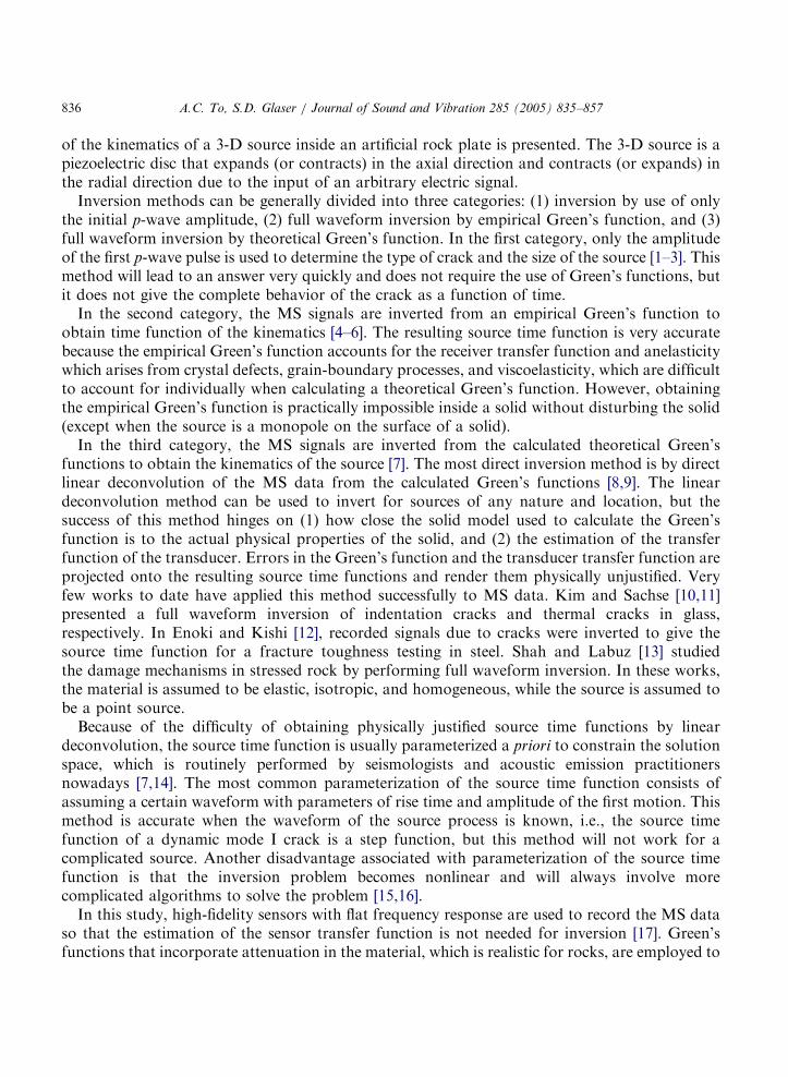
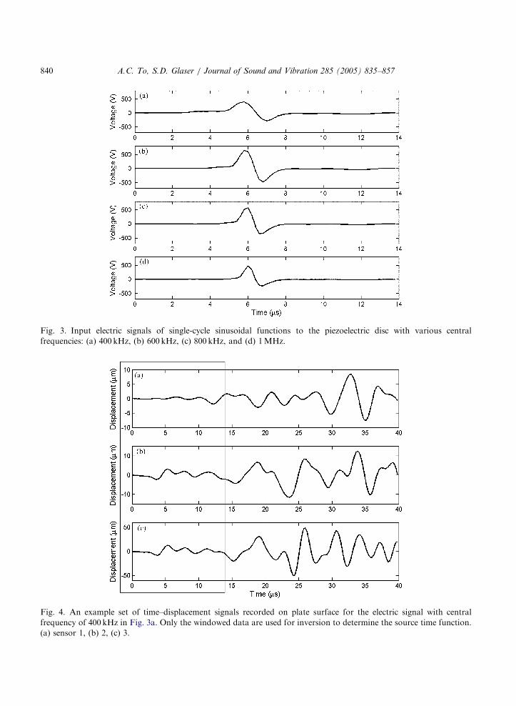
In the experiment, the PZT disc is mechanically deformed by inputting an electric signal and theelastic waves emitted and propagated through the gypsum plate are received by the transducers.The input electric signal is a single cycle sinusoidal wave because of its simplicity and also becausethe resonant behavior of the disc can be observed and analyzed after the input signal becomeszero. A variety of signals having peak-to-peak voltage of 1 kV and bandpassed between 50 kHzand 20MHz, but with different center frequencies, is tested. The input signals of centerfrequencies of 400 kHz, 600 kHz, 800 kHz, and 1MHz are shown in Fig. 3. An example of thetime-displacement waveforms recorded due to the 400 kHz central frequency source is shown inFig. 4. The first p-wave arrives at 0 ms, but the energy from the first p-wave arrival is concentratedbetween 3.5 and 6 ms followed by pp, ppp, ps, and sp arrivals. The first shear wave energy isconcentrated between 19 and 21 ms, but it cannot be clearly discerned because it is blurred by the

ARTICLE IN PRESS

Fig. 3. Input electric signals of single-cycle sinusoidal functions to the piezoelectric disc with various central

frequencies: (a) 400 kHz, (b) 600 kHz, (c) 800 kHz, and (d) 1MHz.

Fig. 4. An example set of time–displacement signals recorded on plate surface for the electric signal with central

frequency of 400 kHz in Fig. 3a. Only the windowed data are used for inversion to determine the source time function.

(a) sensor 1, (b) 2, (c) 3.


ARTICLE IN PRESS


ps and sp wave energies. The energy from the Rayleigh wave is concentrated between 23 and 27ms.A time window of first 14ms after the first p-wave arrival is used for inversion for the source timefunction (Fig. 4). As just discussed, this time window includes the p, pp, ppp, ps, and sp wavearrivals. In the experimental setup, the distance from the source to the closest edge of the plate is254mm, and so the first reflection off the edge is 44ms after the first p-wave arrival. The wavearrives at the edge long after the cutoff time in the inversion, and thus has little effect on thewaveform under consideration. Also, the edge effect on the waveform before the wave reflects offthe edge was shown to be insignificant by Micheals et al. [5], and others [6].

3. The forward problem

The kinematics of a point source can be completely described by a linear combination of nineforce couples or moments (three components of force and three components of arm directions) asshown in Fig. 5 [18]. Literally, the moment tensor Mpq(x,t) is defined as the limit of the product ofthe the qth direction force arm Dxq and the pth direction forcing function Fp(x,t) at location x andtime t [18]:

Mpqðx; tÞ ¼ limDxq!0

Fp!1

DxqFpðx; tÞ; (1)

where Fp is the force time function in the pth direction and Dxq is the force arm in the qthdirection. The moment tensor Mpq(x,t) is symmetric in p and q due to the conservation ofmomentum for an internal source [18], and thus there are six unique moments instead of nine. Thedisplacement time history un(x,t) at location x in the nth direction due to a point source can be

Fig. 5. Nine components of the moment tensor (Aki and Richards, [18]).

ARTICLE IN PRESS


modeled as a convolution integral of the moment tensor and the Green’s displacement tensor:

unðx; tÞ ¼X3

p¼1

X3

q¼1

Gnp;qðx; t; x; 0ÞnMpqðx; tÞ; (2)

where an asterisk denotes a convolution integral in the time variable. The Green’s displacementtensor Gnp,q(x,t,x,0) is the displacement in the nth direction at x and t due to a unit impulsiveconcentrated moment at x and t=0.

Unfortunately, instead of being point sources, cracks have a real extent and the time history ofthe growing crack is of primary interest. For a source over a finite area A, the displacement atlocation x in the nth direction can be obtained by integrating Eq. (2) over A:

unðx; tÞ ¼

ZZS

X3

p¼1

X3

q¼1

Gnp;qðx; t; x; 0ÞnMpqðx; tÞ dA: (3)

According to Johnson and Stump [7], if the region A is discretized into Nr sub-regions whoselargest dimension is smaller than the smallest wavelength of interest, each sub-region i is wellapproximated by a point source. Therefore, summing the contribution from the sub-regions, weobtain

unðx; tÞ ¼XNr

i¼1

X3

p¼1

X3

q¼1

Gnp;qðx; t; xðiÞ; 0ÞnMpqðx

ðiÞ; tÞ: (4)

So far, we have focused on modeling the kinematics of a source whose volume is infinitesimal,but the volume of the actual simulated crack in the experiment is not, and thus the force arm inEq. (1) is no longer infinitesimal. Eq. (4) can be first rewritten as

unðx; tÞ ¼XNr

i¼1

X3

p¼1

X3

q¼1

limDxðiÞq !0

Gnpðx; t; xðiÞþ 0:5DxðiÞq ; 0Þ � Gnpðx; t; x

ðiÞ� 0:5DxðiÞq ; 0Þ

DxðiÞq

0BB@

limDxðiÞq !0

f p!1

DxðiÞq FpðxðiÞ; tÞ

1CCA ð5Þ

and then removing the limits from Eq. (5), we obtain

unðx; tÞ ¼XNr

i¼1

X3

p¼1

X3

q¼1

ðGnpðx; t; xðiÞþ 0:5DxðiÞq ; 0Þ � Gnpðx; t; x

ðiÞ� 0:5DxðiÞq ; 0ÞÞnFpðx

ðiÞ; tÞ

(6)

where Gnp(x,t;x(i),0) is the displacement in the nth direction at x and t due to a unit impulsive

concentrated force at x(i) and t=0. Fp(x(i),t) is the force time function in the pth direction. Eq. (6)

ARTICLE IN PRESS


can be interpreted as the sum of the displacements due to time-variant force couples with finitemoment arms on all the sub-regions.

4. Calculation of Green’s functions

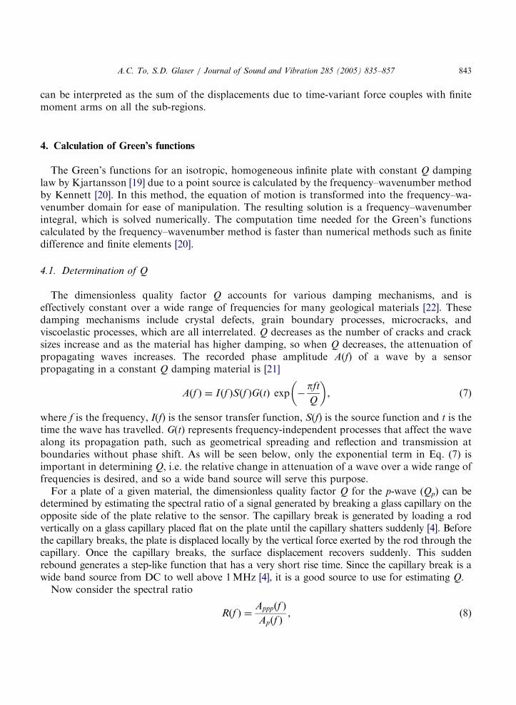
The Green’s functions for an isotropic, homogeneous infinite plate with constant Q dampinglaw by Kjartansson [19] due to a point source is calculated by the frequency–wavenumber methodby Kennett [20]. In this method, the equation of motion is transformed into the frequency–wa-venumber domain for ease of manipulation. The resulting solution is a frequency–wavenumberintegral, which is solved numerically. The computation time needed for the Green’s functionscalculated by the frequency–wavenumber method is faster than numerical methods such as finitedifference and finite elements [20].

4.1. Determination of Q

The dimensionless quality factor Q accounts for various damping mechanisms, and iseffectively constant over a wide range of frequencies for many geological materials [22]. Thesedamping mechanisms include crystal defects, grain boundary processes, microcracks, andviscoelastic processes, which are all interrelated. Q decreases as the number of cracks and cracksizes increase and as the material has higher damping, so when Q decreases, the attenuation ofpropagating waves increases. The recorded phase amplitude A(f) of a wave by a sensorpropagating in a constant Q damping material is [21]

Aðf Þ ¼ Iðf ÞSðf ÞGðtÞ exp �pft

Q

� �; (7)

where f is the frequency, I(f) is the sensor transfer function, S(f) is the source function and t is thetime the wave has travelled. G(t) represents frequency-independent processes that affect the wavealong its propagation path, such as geometrical spreading and reflection and transmission atboundaries without phase shift. As will be seen below, only the exponential term in Eq. (7) isimportant in determining Q, i.e. the relative change in attenuation of a wave over a wide range offrequencies is desired, and so a wide band source will serve this purpose.

For a plate of a given material, the dimensionless quality factor Q for the p-wave (Qp) can bedetermined by estimating the spectral ratio of a signal generated by breaking a glass capillary on theopposite side of the plate relative to the sensor. The capillary break is generated by loading a rodvertically on a glass capillary placed flat on the plate until the capillary shatters suddenly [4]. Beforethe capillary breaks, the plate is displaced locally by the vertical force exerted by the rod through thecapillary. Once the capillary breaks, the surface displacement recovers suddenly. This suddenrebound generates a step-like function that has a very short rise time. Since the capillary break is awide band source from DC to well above 1MHz [4], it is a good source to use for estimating Q.

Now consider the spectral ratio

Rðf Þ ¼Apppðf Þ

Apðf Þ; (8)

ARTICLE IN PRESS


where Ap(f) is the amplitude of the p phase in the frequency (f) domain and Appp(f) is theamplitude of the reflected p phase. Substituting Eq. (7) into Eq. (8) gives

Rðf Þ ¼GpðtpÞ expð�pftp=QpÞ

GpppðtpppÞ expð�pftppp=QpÞ: (9)

Notice that both the sensor transfer function and the source function are cancelled. Taking thenatural logarithm of Eq. (9) gives

ln Rðf Þ ¼ lnGpðtpÞ

GpppðtpppÞ

� �� pDt=Qp f ; (10)

where Dt is the time difference between the p phase arrival and the ppp phase arrival. FromEq. (10) Qp can be estimated from the slope of ln(R(f)) vs. f plot. The time derivative of theepicentral displacement from the average of three glass capillary breaks on the gypsum plate isplotted in Fig. 6. The time derivative of the epicentral displacement is used rather than the originalsignal because the p and the ppp phases can be observed and extracted easily from the signal. Also,note that Eq. (10) is still valid, since taking the time derivative is equivalent to multiplying theoriginal signal by i2pf in the frequency domain, and the factors for the p amplitude and the ppp

amplitude cancel each other in Eq. (8). The natural log of the spectral ratio R(f) of the p and theppp phases as a function of frequency f is plotted in Fig. 7. Qp is estimated to be 70 from linearregression fitting of a straight line through the ln(R(f)) vs. f plot, and it is a typical value fornatural rocks [22].

Fig. 6. Time derivative of the epicentral displacement due to a glass capillary break. The p and ppp phases are indicated

in the figure.

ARTICLE IN PRESS

Fig. 7. The spectral ratio of the ppp and p phases (solid line) and the linear regression line from which qp is estimated

(dashed line).


In principle, the same technique above can be used to estimate Q for the shear wave (Qs), i.e. byreplacing the subscript p with s and ppp with sss in Eqs. (8)–(10). However, the reflected sss

amplitude is very small due to the radiation pattern and is dominated by the p reflections andnoise, so it is impractical to use this technique. However, assuming that no energy dissipationoccurs in pure compression for the p-wave, Qs can be estimated from Qp by Apsel [23]:

Qs ¼4

3

Vs

Vp

� �2

Qp; (11)

where Vp and Vs are the respective p-wave and s-wave velocity.It is simple to include Q damping in the calculation of the Green’s functions by making the

p-wave velocity (Vp) and s-wave velocity (Vs) complex [19]:

V ¼ ðV0Þ cospg2

�

ioo0

� �g (12)

with

g ¼1

parctan

1

Q

� �; (13)

where V is the p-wave or the s-wave velocity. V0 is the reference velocity at frequency o0.

ARTICLE IN PRESS


5. The inverse problem

The goal of the present study is to determine the force time function Fp(x(i),t) in Eq. (6) given

several displacement time histories un(x,t), Green’s functions Gnp(x,t;x(i),0), and the source

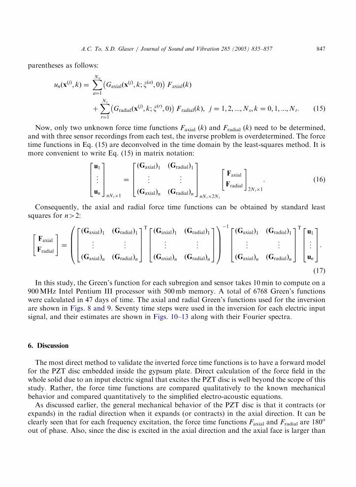
location. In order to formulate the inverse problem for the experiment, the source needs to bediscretized into sub-regions where each subregion is much less than the shortest wavelength ofinterest to be considered a point source effectively [7]. The axial face of the disc is discretized intomostly square sub-regions by 26 equally spaced vertical and horizontal lines, and the largestdimension of each sub-region is 0.52mm. (Fig. 2). The radial face is discretized into 1120 sub-regions whose largest dimension is 0.53mm. Each sub-region is now effectively a point source andthus the Green’s functions for each sub-region can be calculated by the frequency–wavenumbermethod [20]. For the inverse problem, the unknown force time function of each direction for eachsub-region needs to be determined, and that means thousands of sensor signals are needed toperform the inversion. However, the number of unknowns can be reduced substantially byapplying our knowledge of the mechanical behavior of the PZT disc and the gypsum plate. Thefollowing two simplifications are made in the formulation of the inverse problem:

(1)
Each subregion on the axial face can only exert an axial force and each subregion on the radialface can only exert a radial force.
(2)
The axial force time function is identical for each subregion on the axial face and the radialforce time function is identical for each subregion on the radial face.
These simplifications follow directly from the assumption that the bonding between the PZTdisc and the gypsum is smooth (ie. frictionless) and that the disc expands (or contracts) in the axialdirection due to the input of an electric signal and correspondingly contracts (or expands) in theradial direction. With the first simplication, the Green’s function due to an impulsive axial forcefor each sensor (Gaxial (x,t;x,0)) is calculated for each subregion on the axial face, and in thesame manner, the Green’s function due to an impulsive radial force for each sensor (Gradial

(x,t;x,0) is calculated for each subregion on the radial face. The set of equations to be solved canbe written as

unðxðjÞ; kÞ ¼

XNa

a¼1

GaxialðxðjÞ; k; xðaÞ; 0Þ Faxialðx

ðaÞ; kÞ �

þXNr

r¼1

GradialðxðjÞ; k; xðrÞ; 0ÞF radialðx

ðrÞ; kÞ �

; j ¼ 1; 2; :::;Ns; k ¼ 0; 1; :::;Nt ð14Þ

where x(j) is the jth sensor location, Ns is the number of sensors, Na the number of sub-regions onthe axial face, and Nr the number of subregions on the radial face. Since the observeddisplacements are discretized at an interval Dt, the continuous time t in Eq. (6) is replaced byincrement k times Dt. Faxial (x

(a),k) and Fradial (x(r),k) are the axial and radial force time functions

at each subregion on the axial and radial face, respectively. With the second simplification that theforce time function is identical for all the axial subregions and for all the radial subregions,respectively, the axial and the radial force time functions in Eq. (14) can be taken out of the

ARTICLE IN PRESS


parentheses as follows:

unðxðjÞ; kÞ ¼

XNa

a¼1

GaxialðxðjÞ; k; xðaÞ; 0Þ

�FaxialðkÞ

þXNr

r¼1

GradialðxðjÞ; k; xðrÞ; 0Þ

�F radialðkÞ; j ¼ 1; 2; :::;Ns; k ¼ 0; 1; :::;Nt: ð15Þ

Now, only two unknown force time functions Faxial (k) and Fradial (k) need to be determined,and with three sensor recordings from each test, the inverse problem is overdetermined. The forcetime functions in Eq. (15) are deconvolved in the time domain by the least-squares method. It ismore convenient to write Eq. (15) in matrix notation:

u1

..

.

un

2664

3775

nNt�1

¼

ðGaxialÞ1 ðGradialÞ1

..

. ...

ðGaxialÞn ðGradialÞn

2664

3775

nNt�2Nt

Faxial

Fradial

" #2Nt�1

: (16)

Consequently, the axial and radial force time functions can be obtained by standard leastsquares for n42:

Faxial

Fradial

" #¼

ðGaxialÞ1 ðGradialÞ1

..

. ...


2664

3775

TðGaxialÞ1 ðGradialÞ1

..

. ...


2664

3775

0BBB@

1CCCA

�1ðGaxialÞ1 ðGradialÞ1

..

. ...


2664

3775

Tu1

..

.

un

2664

3775:(17)

In this study, the Green’s function for each subregion and sensor takes 10min to compute on a900MHz Intel Pentium III processor with 500mb memory. A total of 6768 Green’s functionswere calculated in 47 days of time. The axial and radial Green’s functions used for the inversionare shown in Figs. 8 and 9. Seventy time steps were used in the inversion for each electric inputsignal, and their estimates are shown in Figs. 10–13 along with their Fourier spectra.

6. Discussion

The most direct method to validate the inverted force time functions is to have a forward modelfor the PZT disc embedded inside the gypsum plate. Direct calculation of the force field in thewhole solid due to an input electric signal that excites the PZT disc is well beyond the scope of thisstudy. Rather, the force time functions are compared qualitatively to the known mechanicalbehavior and compared quantitatively to the simplified electro-acoustic equations.

As discussed earlier, the general mechanical behavior of the PZT disc is that it contracts (orexpands) in the radial direction when it expands (or contracts) in the axial direction. It can beclearly seen that for each frequency excitation, the force time functions Faxial and Fradial are 180o

out of phase. Also, since the disc is excited in the axial direction and the axial face is larger than

ARTICLE IN PRESS

Fig. 8. Green’s functions in the axial direction corresponding to (a) sensor 1, (b) 2, and (c) 3.

Fig. 9. Green’s functions in the radial direction corresponding to (a) sensor 1, (b) 2, and (c) 3.


ARTICLE IN PRESS

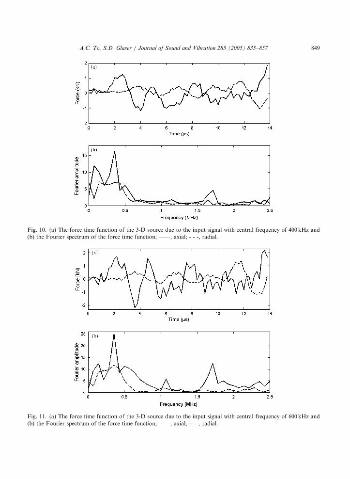
Fig. 10. (a) The force time function of the 3-D source due to the input signal with central frequency of 400 kHz and

(b) the Fourier spectrum of the force time function; ——, axial; - - -, radial.




ARTICLE IN PRESS



Fig. 13. (a) The force time function of the 3-D source due to the input signal with central frequency of 1MHz and

(b) the Fourier spectrum of the force time function.


ARTICLE IN PRESS


the radial face, the axial force time function Faxial is expected to be larger in amplitude than theradial force time function Fradial, which is shown to be the case for each input signal. To determinehow accurate the force time functions are for each case, the change in thickness and diametercalculated from the first peak input voltage can be compared to those calculated from the forcefrom the first peak in the force time function, which corresponds to the first peak input voltage.The change in thickness Dh due to an input voltage V is

Dh ¼ d33V (18)

and the change in diameter DD due to an input voltage V is

DD ¼d31D

hV ; (19)

where d33 and d31 are piezoelectric constants (Table 1). The changes in thickness and in diameterdue to applied forces are obtained from the stress–strain relationship by converting the forces intostresses in the axial and radial directions. Adopting the abbreviated notations from Auld [24], thestress–strain relationship is

SI ¼ sE;CIJ TJ ; (20)

where SI and TJ are strains and stresses and sEIJ and sC

IJ are the compliances measured in constantelectric field and in constant charge density, respectively (Table 1). Because of the couplingbetween electric and acoustic fields in the PZT disc, measurement of the mechanical propertiesdepends on the electrical constraints [24]. The dynamic electric field within the PZT disc isunknown during the experiment, so the compliances measured in a constant electric field and inconstant charge density are used to calculate the changes in thickness and in diameter. The resultsare tabulated in Table 2, where positive sign denotes extension and negative sign denotescontraction. For each input electric signal, the changes in thickness and in diameter calculatedfrom the peak forces are larger than those calculated from the peak voltage. The discrepanciesmay be due to the fact that the simple calculations above assume idealized boundary conditionsand static mechanical and electrical behavior, while the real behavior is dynamic; but the changesin thickness and diameter calculated from the peak forces and from the peak voltage are of thesame order of magnitude. Also observed from the table is that the change in thickness is alwayslarger than the change in diameter because the disc is excited axially. As expected, the larger thepeak voltage, the larger the changes in thickness and in diameter, and this fact is also reflected inthe calculation from the peak forces.

The dynamic mechanical behavior of the source can be studied from the waveform of the forcetime functions. The waveform of the force time functions from 0 to 4 ms looks quite similar to theirrespective input electric signals in Fig. 3 while the later part of all the force time functionsoscillates with varying amplitudes at different frequencies. This is to be expected since the PZTdisc is known to resonate due to electrical excitation, and the frequencies at which it resonates canbe seen from the Fourier spectra of the force time functions. In all cases, it is apparent that threepeaks in the Fourier spectra are at the same frequencies: 0.32, 1.1 and 1.7MHz, while two peaksthat occur at the same frequencies are not as apparent: 0.63 and 0.95MHz.These results can beexplained by the axial normal modes of the PZT disc, assuming axial faces are stress free. Thisassumption is acceptable because the disc is excited axially and the axial p-wave impedance of

ARTICLE IN PRESS

Table 2

Deformation of the source calculated from the peak forces and peak voltage

Input electrical signal

central frequency

(MHz)

Peak axial

force (N)

Peak radial

force (N)

Change in

thicknessE

(mm)

Change in

thicknessC

(mm)

Change in

diameterE

(mm)

Change in

diameterC

(mm)

0.4 1240 �45 1.05 0.52 �0.81 �0.36

0.6 1720 �90 1.46 0.73 �1.16 �0.54

0.8 1560 �34 1.31 0.66 �0.98 �0.43

1 1400 �110 1.20 0.60 �1.00 �0.49

Input electrical signal central frequency (MHz) Peak voltage (V) Change in thickness (mm) Change in diameter (mm)

0.4 346 0.13 �0.11

0.6 622 0.23 �0.20

0.8 586 0.22 �0.19

1 482 0.18 �0.15

ECalculated from compliances measured in constant electric field.CCalculated from compliances measured in constant density charge.


piezoelectric solid (rVp=29.3MPa s/m3) is almost three times higher than that of gypsum (rVEpa

=11.0MPa s/m3), whereVEpa is the axial p-wave velocity measured in a constant electric field. The

axial normal modes are the solutions to the following equation:

sinðpf nh=VpaÞ ¼ 0; cosðpf nh=VpaÞ ¼ 0; (21)

which have solutions

f n ¼ nVpa=2h; n ¼ 1; 2; 3; . . . ; (22)

where fn are the normal modes, h is the thickness of the PZT disc and Vpa is the axial p-wavevelocity. The first five modes observed from the Fourier spectra in Figs. 10–13 and the modescalculated from Eq. (22) with two different Vpa measured in a constant electric field and inconstant charge density are tabulated in Table 3. Note that all five modes calculated from Eq. (22)are slightly smaller than those observed from the peaks in the Fourier spectra in all cases. Thedifference is expected since the actual boundary conditions of the disc are not truly stress free as inthe calculations, and also there may be other modes in addition to the axial modes being excited.

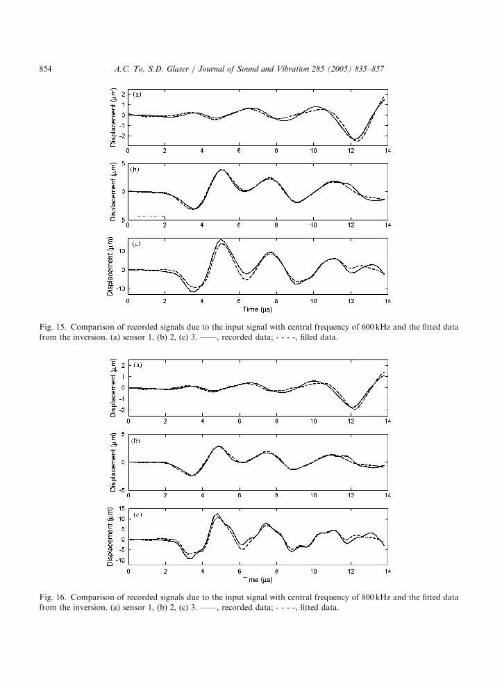
The fitted data in Figs. 14–17 are obtained by convolving the Green’s functions with the forcetime functions through Eq. (17). Since the inverse problem is overdetermined and is solved byleast squares, the fitted data are not necessarily identical to the recorded data and so it ismeaningful to compare them to examine the misfit. In each case, the fitted data have a good matchwith the original recorded data. There may be several sources that lead to the very slight misfit.First, the Green’s function calculated based on Q damping may not truly capture theinhomogeneity in the gypsum plate and all the damping processes during wave propagation.Second, the Green’s function is calculated assuming each sub-region is a point source, and the

ARTICLE IN PRESS

Fig. 14. Comparison of recorded signals due to the input signal with central frequency of 400 kHz and the fitted data

from the inversion. (a) sensor 1, (b) 2, (c) 3. ——, recorded data; - - - -, filled data.

Table 3

Axial normal modes of the PZT disc

Modes (MHz)

n=1 n=2 n=3 n=4 n=5

Calculated from normal mode theoryE 0.26 0.53 0.79 1.1 1.3

Calculated from normal mode theoryC 0.30 0.61 0.91 1.2 1.5

Observed from the Fourier spectra of the

force time functions

0.32 0.63 0.95 1.1 1.7

ECalculated from axial p-wave velocity measured in constant electric field (see Table 1).CCalculated from axial p-wave velocity measured in constant density charge (see Table 1).


error in the Green’s function grows with increasing frequency [7]. However, from the good matchbetween the fitted data and the recorded data, these errors are deemed to be minor.

The very long computation time (47 consecutive days) used to calculate all the Green’sfunctions raises the question of the practicality of the current method. The computation can bemade more efficient by a change of platform and integration algorithm. Since the current code isin written in Matlab running in Windows 2000, it is believed that the computation time can bereduced by well more than 50% if the code were written in Fortran or in C running on a Linuxplatform. In addition, the numerical integration of the wavenumber integral in Kennett’s method

ARTICLE IN PRESS


from the inversion. (a) sensor 1, (b) 2, (c) 3. ——, recorded data; - - - -, fitted data.




ARTICLE IN PRESS

Fig. 17. Comparison of recorded signals due to the input signal with central frequency of 1MHz and the fitted data



[20] is performed by Simpson’s rule. A more efficient scheme can be developed by approximatingthe integrand by Chebyshev polynomials as performed by Xu and Mal [25], but this requires sometesting to make the method work well. A new Windows-based computer will nominally run aboutfive times faster than the older machine used for this paper.

7. Conclusions

In this study, we have successfully used theoretical Green’s functions incorporating Q dampingto perform a full waveform inversion. There are three crucial factors that we believe lead to thesuccessful inversion: (1) the use of broadband transducers with high-fidelity frequency response,(2) the use of Green’s functions based on Q damping, and (3) taking the source finiteness intoaccount. The use of narrowband transducers requires obtaining the transfer function each time atest is performed on a different solid and then performing deconvolution of the microseismic datafrom the transfer function. Since a narrowband transducer has missing data in some frequencies,the deconvolution is fundamentally ill-posed. For broadband transducers, all displacementinformation present is being transduced and is included in the inversion.

The microseismic data are inverted from inelastic Green’s functions, rather than based on alinear, homogenous, elastic solid model. For a plate, Q can be obtained experimentally by

ARTICLE IN PRESS


breaking a capillary on one side of the plate. It captures the damping behavior of the gypsumquite well.

This study also incorporates the source finiteness in formulating the inverse problem. Since thesource size is known a priori, the disc can be discretized into subregions with the largest dimensionless than the minimum wavelength such that each subregion is effectively a point source. This isbelieved to improve the accuracy of the Green’s functions and consequently lead to betterinversion results.

The success of a full waveform inversion is judged by whether the inverted results can beexplained physically. The inverted force time functions match the known mechanical behavior ofthe PZT disc and the observed oscillations match well with the theoretical axial normal modes.

Although the use of high–fidelity sensors, the calculation of the Green’s function that includesdamping, the summation of point sources into finite sources, and the technique of inversion areeach not new, the incorporation of all the above to obtain physically justified source timefunctions for a complex source is a new development in microseismic inversion. It should beemphasized that in this study the source time function is not parametrized a priori like manyseismologists and acoustic emission researchers do nowadays to obtain physical solutions. Fordynamic crack inversion, it is certainly fine to assume the waveform of the source time function tobe a step function. In more complicated dynamic processes such as in this study, directdeconvolution must be used to determine the source processes. In fact, recently the source timefunction on a subfault calculated based on an asperity model for dynamic earthquake faultingshows more than a step function: the source time function is actually a step function, followed byperiodic undulations [26]. If the parameterization of a step function is used for inversion, the realbehavior of the source process will not be obtained. Another problem associated with theparameterization of the source time function is that the inversion problem becomes nonlinear andwill always involve more complicated algorithms to solve the problem. In conclusion, this studydemonstrates the feasibility of obtaining the most complete and physically justified quantitativeinformation from a dynamic source process in a damped solid.

Acknowledgements

This research is supported by NSF project CMS-9908218, ‘Multi-Scale ExperimentalInvestigation of Sliding Friction.’

References

[1] C.B. Scruby, G.R. Baldwin, K.A. Stacey, Characterisation of fatigue crack extension by quantitative microseismic,

International Journal of Fracture 28 (1985) 201–222.

[2] C.B. Scruby, K.A. Stacey, G.R. Baldwin, Defect characterisation in three dimensions by acoustic emission, Journal

of Physics D: Applied Physics 19 (1986) 1597–1612.

[3] M. Ohtsu, Simplified moment tensor analysis and unified decomposition of acoustic emission source: application

to in situ hydrofracturing test, Journal of Geophysical Research 96 (1991) 6211–6221.

[4] F.R. Breckenridge, T.M. Proctor, N.N. Hsu, S.E. Fick, D.G. Eitzen, Transient sources for acoustic emission work,

Procceedings of the 10th International Acoustic Emission Symposium, Tokyo, 1990, pp. 20–37.

ARTICLE IN PRESS


[5] J.E. Michaels, T.E. Michaels, W. Sachse, Applications of deconvolution to microseismic signal analysis, Materials

Evaluation 39 (1981) 1032–1036.

[6] S.D. Glaser, P.P. Nelson, Acoustic emissions produced by discrete fracture in rock—part 2: kinematics of crack

growth during controlled Mode I and Mode II loading of rock, International Journal of Rock Mechanics 29 (1992)

253–265.

[7] T. Lay, T. Wallace, Modern Global Seismology, first ed, Academic Press, San Diego, 1995.

[8] B.W. Stump, L.R. Johnson, The determination of source properties by the linear inversion of seismograms,

Bulletin of the Seismological Society of America 67 (1977) 1489–1502.

[9] R.A. Strelitz, Moment tensor inversions and source models, Geophysical Journal of the Royal Astronomical Society

52 (1978) 359–364.

[10] K.Y. Kim, W. Sachse, Acoustic emissions from penny-shaped cracks in glass—part II: Moment tensor and

source–time function, Journal of Applied Physics 59 (1986) 2711–2715.

[11] K.Y. Kim, W. Sachse, Characteristics of an microseismic source from a thermal crack in glass, International

Journal of Fracture 31 (1986) 211–231.

[12] M. Enoki, T. Kishi, Theory and analysis of deformation moment tensor due to microcracking, International

Journal of Fracture 38 (1988) 295–310.

[13] K.R. Shah, J.F. Labuz, Damage mechanisms in stressed rock from acoustic emission, Journal of Geophysical

Research 100 (1995) 15527–15539.

[14] T. Kishi, M. Ohtsu, S. Yuyama (Eds.), Acoustic Emission—Beyond the Millennium, Elsevier, New York, NY, 2000.

[15] S.H. Hartzell, T.H. Heaton, Inversion of strong ground motion and teleseismic waveform data for the fault

rupture history of the 1979 Imperial Valley, California, earthquake, Bulletin of the Seismological Society of

America 73 (1983) 1553–1583.

[16] J.E. Michaels, Y.H. Pao, The inverse problem for an oblique force on an elastic plate, Journal of the Acoustical

Society of America 77 (1985) 2005–2011.

[17] S.D. Glaser, G. Weiss, L.R. Johnson, Body waves recorded inside an elastic half space by an embedded wideband

velocity sensor, Journal of the Acoustical Society of America 104 (1998) 1404–1412.

[18] K. Aki, P.G. Richards, Quantitative Seismology, Theory and Method, second ed., University Science Books,

Sausalito, CA, 2000.

[19] E. Kjartansson, Constant Q-wave propagation and attenuation, Journal of Geophysical Research 84 (1979)

4737–4748.

[20] B.L.N. Kennett, Seismic Wave Propagation in Stratified Media, Cambridge University Press, Cambridge, UK,

1983.

[21] M. Niazi, L.R. Johnson, Q in the inner core, Physics of the Earth and Planetary Interiors 74 (1992) 55–62.

[22] L. Knopoff, Q, Review of Geophysics 2 (1964) 625–660.

[23] R. Apsel, Dynamic Green’s functions for layered media and applications to boundary-value problems, Ph.D.

Thesis, University of California, San Diego, 1979.

[24] B.A. Auld, Acoustic Fields and Waves in Solids (two volumes), second ed., Krieger Publications, Florida, 1990.

[25] P. Xu, A.K. Mal, An adaptive integration scheme for irregularly oscillatory functions, Wave Motion 7 (1985)

235–243.

[26] L.R. Johnson, R. Nadeau, An asperity model of an earthquake: dynamic problem, Bulletin of the Seismological

Society of America, in press.

Documents

Full waveform inversion of a 3-D source inside an …glaser.berkeley.edu/glaserdrupal/pdf/JSV 2005.pdfJOURNAL OF SOUND AND VIBRATION Journal of Sound and Vibration 285 (2005) 835–857