Confidential manuscript submitted to Water Resource Research

Draft of Nov 21, 2015

Design and evaluation of a basin-scale wireless sensor network for mountain hydrology

Z. Zhang1, S. Glaser1, R. Bales1,2, M. Conklin2, R. Rice2 and D. Marks3

1Department of Civil and Environmental Engineering, University of California, Berkeley,

Berkeley, USA. 2Sierra Nevada Research Institute and School of Engineering, University of California, Merced,

Merced, USA. 3Agricultural Research Service, USDA, Boise, USA.

Ziran Zhang (zhangziran@berkeley.edu) Steven Glaser (glaser@berkeley.edu) Roger Bales (rbales@ucmerced.edu) Martha Conklin (mconklin@ucmerced.edu) Robert Rice (rrice@ucmerced.edu) Danny Marks (ars.danny@gmail.com)

Key Points:

• We designed and deployed a robust basin-scale wireless-sensor network for spatially distributed water-balance measurements across American River basin.

• The variability of snow, temperature, and humidity within 1-km2 forested clusters was near 200-800 m elevation difference.

• The distributed sensor provided unprecedented detail on patterns of rain vs. snow, and differed significantly from point measurements at met stations.

Confidential manuscript submitted to Water Resource Research

Draft of Nov 21, 2015

Abstract 1

A basin-scale instrument for spatially representative water-balance measurements was 2

developed and deployed in the upper, snow-dominated portion of the American River basin, 3

primarily to measure changes in snowpack and soil-water storage, temperature and humidity. 4

This wireless sensor network (WSN) consists of 14 sensor clusters spread over the 2000 km2 part 5

of the basin above 1500-m elevation. Each cluster has 10 measurement nodes that were 6

strategically placed within a 1-km2 area, across different elevations, aspects, slopes and 7

vegetation densities. Considerable spatial variability was apparent in within-cluster 8

measurements of temperature, relative humidity and snow depth, comparable to that across the 9

basin. This variability capturing the importance of aspect and forest density on ground-level 10

temperature and precipitation, snow accumulation and melt, and atmospheric-water content. 11

Results also showed notable differences between spatially averaged WSN measurements within 12

a cluster, as compared to single-point measurements at a met station or snow pillow, or to spatial 13

estimates of snow accumulation and melt derived from operational data. Distributed dew-point 14

temperature and snow depth data were used to develop an estimate of the fraction of rain vs. 15

snow across the upper basin. Network statistics during the first year of operation demonstrated 16

that the WSN was robust for cold, wet and windy conditions in the basin. The technology used 17

in the WSN reduced adverse effects, such as, high current consumption, multipath signal fading 18

and clock drift, seen in previous remote WSN. 19

Index Terms and Keywords: 20

Wireless sensor network, water information system, snow observation, mountain hydrology, 21

rain/snow transition, American River. 22

23

3

1 Introduction 24

Measurement of mountain water cycles at the basin scale are limited in both spatial 25

coverage and temporal resolution, with data largely provided by a few operational precipitation, 26

snowpack, climate and stream-gauging stations [Bales et al., 2006; Dozier, 2011]. In the Sierra 27

Nevada, measurement sites tend to be limited to middle and lower elevations and flat terrain in 28

forest clearings [Molotch and Bales, 2005]. Research networks include a few selected headwater 29

basins where a more complete set of meteorological and hydrologic attributes are accurately 30

measured [Kerkez et al., 2012] on a limited scale. While these catchments offer some detailed 31

information on mountain hydrology, they provide a limited understanding of the hydrology of 32

larger mountain river basins that can be characterized by steep gradients in temperature, 33

precipitation, rain versus snow fraction, growing season, vegetation density and 34

evapotranspiration. Climate warming is raising the rain-snow transition elevation and changing 35

the hydrologic response of mountain basins. While we can describe these changes in larger 36

mountain basins in general terms using data from research catchments [Goulden and Bales, 37

2014], developing the dense time series of spatial variables needed to drive the next generation 38

of forecast tools remains a challenge [Klemes, 1987; Dressler et al., 2006]. 39

Detailed quantification of the water balance at finer spatial and smaller temporal 40

resolutions is also critical to research in atmospheric science, biogeochemistry, ecosystem 41

science, water resources, and is central to research in hydrologic science [NRC, 2008]. A richer 42

dataset will allow us to understand and characterize the critical gradients in temperature, 43

humidity, wind, and precipitation volume and phase that define the dynamics of mountain 44

hydroclimatology during this period of rapid climate warming and change. It will enable use of 45

new classes of spatially explicit hydrologic-modeling tools to produce quantitative assessments, 46

4

influence hydrologic forecasting, probe system response to climate and land-cover perturbations, 47

increase process understanding of basin-scale water cycles, and provide defensible scenarios for 48

infrastructure planning over a scale currently not possible. 49

The two main stores of water in mountain basins, snowpack and regolith water storage, 50

are highly variable and not readily estimated by the index sampling characteristic of operational 51

hydrology [Molotch and Bales, 2006; Bales et al., 2011]. Snow accumulation and melt are also 52

highly variable [Molotch et al., 2004, 2005], with melt providing a spatially variable input to soil 53

moisture, or subsurface storage. Depletion of subsurface storage through drainage and 54

evapotranspiration are also highly variable [Bales et al., 2011]. While these quantities can be 55

simulated at various spatial scales, the data to evaluate the spatial accuracy of the modeling is 56

sorely lacking. Thus development of spatially distributed measurement networks, using strategic 57

sampling to capture the main variables influencing spatial patterns of the mountain water balance 58

offers the potential to transform the resolution and accuracy of data for hydrologic forecasting. 59

The most practical method for collecting continuous ground-based data over large areas 60

is the use of wireless sensor networks (WSN). Areas on the scale of square kilometers can easily 61

be covered, which would be impossible using wired sensor arrays. Adopting wireless solutions 62

is enabled by reduced production costs of wireless equipment, advances in development of 63

networking protocols, and the synergies that wireless technology creates by combining 64

traditionally non-wireless sensing equipment with a wireless platform. [Akyildiz et al., 2002; 65

Yick et al., 2008; Gilbert, 2012]. Over the last ten years WSNs have been deployed over various 66

spatial scales, showing some successes in monitoring environmental attributes with distributed 67

arrays of sensors. Dozens, sometimes hundreds of wireless sensor nodes hosting non-trivial 68

numbers of sensors were put into outdoor environments to measure and monitor air temperature, 69

5

relative humidity, snow depth [Kerkez et al., 2012], soil moisture [Bogena et al., 2010; Rice and 70

Bales, 2010; Li and Serpen, 2012], permafrost [Hasler et al., 2008], forest fire [Hartung et al., 71

2006]; potential landslides [Terzis et al., 2006] and volcanic activities [Werner-Allen et al., 72

2006]. The use of WSNs and actuators for monitoring and controlling various aspects of 73

agricultural activities, such as temperature and irrigation schedule, have also gained tremendous 74

attention over the years [Beckwith et al., 2004; Evans and Iversen, 2008; Gutierrez et al., 2014]. 75

Earlier campaigns using WSNs for habitat monitoring have shown both the opportunities 76

offered by spatially and temporally dense data and technical challenges due to unrealizable 77

network performances in applying this new technology to environmental monitoring 78

[Mainwaring et al., 2002; Szewczyk et al., 2004]. A 12-station deployment, from June to 79

October 2009, in a 20-km2 catchment in the Swiss Alps measured the spatial variability of 80

meteorological forcing, including temperature and precipitation. However, the study was only 81

conducted over a short time period with rather sparsely distributed stations [Simoni et al., 2011]. 82

Recently, densely deployed sensor arrays have been scaled to a size comparable to the mountain 83

areas being studied. Ninety nine sensor loggers, within three 40-180 km2 basins, were deployed 84

to monitor snow cover dynamics in southern Germany for one winter. However, the system 85

deployed used data loggers rather than a WSN [Pohl et al., 2014]. In another study, 150 wireless 86

nodes with over 600 soil-moisture sensors were installed in a forest catchment at Westebach, 87

Germany to study the spatiotemporal distribution of soil moisture over complex terrain [Bogena 88

et al., 2010]. The study used a variation of ZigBee motes developed by JenNet Ltd. Over 300 89

sensors hosted by 60 wireless nodes are deployed at the Southern Sierra Critical Zone 90

Observatory to study heterogeneous interactions of water within the snowpack, canopy and soil 91

influence on the water cycle [Kerkez et al., 2012]. However, these studies have not yet provided 92

6

quantifiable assessments of network design operation and results at the river-basin scale. A 93

comparison of the existing solutions and technologies for wireless radio is kept in supporting 94

information (Text S1). 95

The aims of the research reported in this paper were to design, deploy and evaluate a 96

spatially distributed basin-scale WSN for remote hydrologic measurements. The evaluation 97

included both the technical reliability of the WSN for providing data and the resulting spatial 98

patterns of attributes measured by WSNs to produce measurements of finer granularity in 99

complex terrain. 100

2 Methods 101

A WSN made up of clusters of wireless-sensor nodes was deployed at 14 sites in 102

strategically chosen locations in the American River basin and evaluated using data from the first 103

eight months of the 2014 water year (Oct-May). Data from the WSN were compared to 104

operational data and Snow Data Assimilation System (SNODAS) product developed by the 105

National Operational Hydrologic Remote Sensing Center to evaluate the effectiveness of the 106

WSN in capturing spatial differences across the basin. The distributed basin-scale measurements 107

established a dew-point temperature based rain/snow transition zone along the elevation transect. 108

Using the calculated dew-point temperature, the rate of snow precipitation from WSN was 109

adjusted with dew-point temperature during the storms, which provided a profile of total rate of 110

precipitation. 111

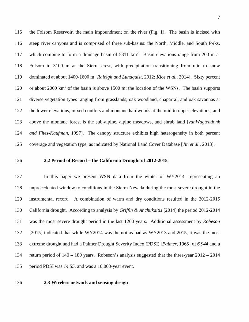
2.1 Study area 112

The study was conducted in the upper, snow-dominated part of the American River basin 113

on the western slope of the Sierra Nevada in California (36.069 N, -120.583 W), located above 114

7

the Folsom Reservoir, the main impoundment on the river (Fig. 1). The basin is incised with 115

steep river canyons and is comprised of three sub-basins: the North, Middle, and South forks, 116

which combine to form a drainage basin of 5311 km2. Basin elevations range from 200 m at 117

Folsom to 3100 m at the Sierra crest, with precipitation transitioning from rain to snow 118

dominated at about 1400-1600 m [Raleigh and Lundquist, 2012; Klos et al., 2014]. Sixty percent 119

or about 2000 km2 of the basin is above 1500 m: the location of the WSNs. The basin supports 120

diverse vegetation types ranging from grasslands, oak woodland, chaparral, and oak savannas at 121

the lower elevations, mixed conifers and montane hardwoods at the mid to upper elevations, and 122

above the montane forest is the sub-alpine, alpine meadows, and shrub land [vanWagtendonk 123

and Fites-Kaufman, 1997]. The canopy structure exhibits high heterogeneity in both percent 124

coverage and vegetation type, as indicated by National Land Cover Database [Jin et al., 2013]. 125

2.2 Period of Record – the California Drought of 2012-2015 126

In this paper we present WSN data from the winter of WY2014, representing an 127

unprecedented window to conditions in the Sierra Nevada during the most severe drought in the 128

instrumental record. A combination of warm and dry conditions resulted in the 2012-2015 129

California drought. According to analysis by Griffin & Anchukaitis [2014] the period 2012-2014 130

was the most severe drought period in the last 1200 years. Additional assessment by Robeson 131

[2015] indicated that while WY2014 was the not as bad as WY2013 and 2015, it was the most 132

extreme drought and had a Palmer Drought Severity Index (PDSI) [Palmer, 1965] of 6.944 and a 133

return period of 140 – 180 years. Robeson’s analysis suggested that the three-year 2012 – 2014 134

period PDSI was 14.55, and was a 10,000-year event. 135

2.3 Wireless network and sensing design 136

8

In 2013-2015, 14 clusters of wireless nodes were deployed in the American River 137

Hydrologic Observatory (Fig. 1, Table 1), with locations selected to represent the range of 138

elevation, aspect, canopy coverage, and potential total and representative solar loading in the 139

basin. All sites, except MTL and DOR, are co-located with existing snow and meteorological 140

sites managed by water and hydropower agencies that have archived historical data. Each of the 141

clusters consists of ten measurement nodes that have snow depth, near-surface air-temperature, 142

and relative-humidity sensors recording at 15-minute intervals, and seven to 35 signal-repeater 143

nodes at each cluster. A Table with equipment used at each site is in supplemental information 144

(Table S1). In this study, data from 10 networks will be discussed, as the other four to be 145

installed do not have data for the year (Table 1). 146

Measurement-node placement consisted of three steps. First step was the evaluation of 147

existing measurement infrastructure in the North, Middle and South Forks. Since precipitation 148

and air temperature are strongly correlated with elevation, sites were identified that would best 149

supplement sampling along elevation transects, while leveraging existing meteorological stations 150

and communication infrastructure in the three sub-basins. The result is a more-thorough 151

distribution of snow sensors across the elevation transect compared to existing snow pillows 152

(Fig. 2). A 1-km2 area around each site was characterized by major physiographic variables that 153

affect the water balance (elevation, slope, aspect, radiation, and canopy cover). [Balk and Elder, 154

2000; Erxleben et al., 2002; Anderton et al., 2004; Essery and Pomeroy, 2004; Sturm and 155

Benson, 2004; Erickson et al., 2005; Marchand and Killingtveit, 2005; Bales et al., 2006]. These 156

site attributes were then expanded to describe the larger basin, and three sub-basins, to assess 157

their representativeness. See supplemental information for the distribution of attributes at each 158

cluster. 159

9

Second step, at each 1-km2 site, ten points representing different terrain attributes were 160

selected by a random stratified technique [Rice and Bales, 2010]. Aggregating the physiographic 161

features represented by each point, cumulative distribution functions were developed for each 162

feature (i.e. aspect, vegetation, slope, total solar loading), and compared to those for the larger 163

basin and the three sub-basins. Rice and Bales [2010] showed that the local-cluster sampling 164

technique, using a 10-sensor measurement network, could effectively capture the mean value of 165

snow depth of an area; and capturing the distribution of snow depths depends on placement. 166

Third step, final location adjustments were made in the field to a small subset of sensor 167

nodes, ensuring a complete sampling of the physiographic features together with a strong WSN 168

connection mesh. Additional technical information on the WSN and its components are 169

provided in the supplemental information. Final system hierarchy is shown schematically in Fig. 170

S2. 171

Each sensor node deployed (Fig. S3) is equipped with an ultrasonic snow-depth sensor 172

(Judd Communication Depth Sensor) and a temperature/relative humidity sensor (Sensirion 173

SHT-15). A selected subset of the nodes at five of the sites measure soil moisture and soil 174

temperature (Decagon GS3) at depths of 10 and 60 cm. Nine sites include measurements of total 175

incoming solar radiation using an upward-pointing Hukseflux-LP02 pyranometer at node 176

locations on a separate mast with a concrete foundation. The solar-radiation sensors at these 177

locations are located in the open, without obstruction by either canopy or the terrain to capture 178

the total available incoming solar irradiance. At 6 of 9 sites, co-located with the clear sky 179

irradiance, solar radiation is measured in a partially canopy-covered location, providing 180

representative solar irradiance measurements underneath the canopy structure. Data from 10 out 181

of 14 sites, covering snow depth, air temperature and relative humidity, for water year 2014 are 182

10

introduced and evaluated in this paper. The other four sites were installed during summer of 183

2014 and 2015. Note, the network statistic data presented in this paper cover a measurement 184

period of about 7 months, while the hydrologic data cover only the first eight months of the 185

water year 2014. The network infrastructure underwent a series of retrofit and upgrades during 186

summer of 2014, and the data record was partially discontinued during the last four months, 187

therefore excluded from this analysis. 188

The wireless network at each local cluster was established in two phases. First was a 189

connecting phase. After sensor motes and the base station were installed; the network manager 190

attempted to populate the network with the sensor and repeater nodes that attempted to join the 191

network. Due to sparsely located sensor nodes, only a subset of the nodes joined in this initial 192

step. In the second phase, signal-repeater nodes were inserted at intermediate locations, 193

following a data guided trial-and-error approach, to connect all of the sensor nodes to the 194

manager with multiple links. Detailed network statistics data, regard to connection strength and 195

network health, were reported in real-time at the base station during deployment to help guide 196

the placement of the signal repeaters, as reinforcement, at key locations to provide a fully 197

meshed redundant network. The general strategy for the reinforced network was to make sure 198

each node had at least two if not three good upstream neighbors. RSSI (Received Signal 199

Strength Indicator) was used as the networking metric to ensure robust link quality in the path to 200

manager, with a factory-prescribed threshold of > -85dBm. 201

2.4 Data evaluation 202

Each node provided 15-minute data for snow depth, temperature and relative humidity. 203

Hourly and daily products were developed for periods where no less than 75% of data were 204

11

present and valid within the averaging window. Extreme values in the data were removed 205

following protocols described in [Daly et al., 2008]. 206

In order to convert snow depth to a snow water equivalent (SWE) measurement, we used 207

a basin-averaged snow density derived from ten snow-telemetry sites where snow depth and 208

SWE were simultaneously measured. Daily data were downloaded 209

(http://www.wcc.nrcs.usda.gov/) from those stations for water year 2014 and a density time 210

series constructed using the ratio of daily SWE and snow depth (Fig. S4). Density values from 211

all sites were averaged, and this mean density time series used for SWE calculations of all WSN 212

nodes, with mean values ranging from about 130 kg m-3 in Jan to 420 kg m-3 in May. Density 213

data at the beginning and the end of the season when the snow pillow may not have been 214

completely covered were omitted. There was no apparent elevation pattern to the density record. 215

Snow density during this period was assumed to be 330 kg m-3, the seasonal average. Near the 216

end of the season, the last valid snow-density value from each site was extended to calculate 217

basin-average snow density. 218

SNODAS data was used as one point of comparison with our snow measurements 219

(http://nsidc.org/data/). Gridded SNODAS data were extracted from cells overlapping WSN 220

clusters using a simple weighted-average scheme (Fig. S5). This daily, spatial dataset is 221

developed from remote, airborne and ground-based station data, providing daily snow depth and 222

SWE estimates. The spatial resolution of the dataset is 1-km [Clow et al., 2012; Guan et al., 223

2013]. Gridded SNODAS daily data for the water year 2014 were also obtained from NSIDC. 224

Snow-depth and SWE features of each node were extracted to the nearest pixel from the daily 225

product. The results of the extracted values from all 10 nodes are averaged to yield the 226

SNODAS mean for each local cluster. 227

12

2.5 Lapse rate of air and dew-point temperature 228

Lapse rates of temperature were established using least-squares regression on daily 229

averaged temperature. Data collected from 81 available sensor nodes were used to compute 230

daily lapse rates of air and dew-point temperature for the upper basin. With relative humidity 231

data, hourly dew-point temperature for each node was computed based on an empirical formula 232

[Lawrence, 2005]. We computed the elevation of the 0oC dew-point temperature, as an 233

indication of where the rain/snow transition potentially occurred, using linear interpolation. 234

2.6 Patterns of snow and total precipitation 235

Positive components of daily differenced WSN SWE were processed to use as the basis 236

of snow precipitation. The rate of snow precipitation for a multi-day event was computed by 237

summing the daily event precipitations for the duration of the entire storm. There were some 238

subjective judgments made to determine if a multi-day storm was a single event or multiple 239

events. The differences were minor due to the overall low intensity of those storms. For each 240

day where precipitation as snow was recorded, the mean dew-point temperatures were examined 241

to determine the phase of precipitation. The proportion of liquid and solid precipitation was 242

developed if the daily dew-point temperature fell between -1 to 1oC. Thresholds were set at -1 243

and 1oC dew-point. Precipitation was considered as 100% solid and 100% liquid if computed 244

mean dew-point temperature were below and above the thresholds of -1 to 1oC. The proportion 245

from solid to liquid varies linearly between the thresholds [Raleigh et al., 2013]. Solid 246

precipitation was then scaled based on the proportionality, to reflect total precipitation. 247

3 Results 248

3.1 WSN performance 249

13

The wireless-network links formed a redundant multi-hopped mesh network of sensors 250

and repeaters for data transport. Fig. 3 shows the stable layout of sensor nodes for one cluster 251

(ALP), and illustrates how repeaters were non-uniformly distributed to connect the sensor nodes 252

via at least two independent paths to the base station. See Fig. S6 for actual photographs of base 253

station, nodes and repeater at ALP. A relatively large number of repeaters were installed to 254

provide redundant paths to sensor nodes 6, 8, and 9, where a steep change in slope produced a 255

radio path kink and reliable network links were challenging to establish. Over time, the 256

topography of the network can change due to a status change of one or more nodes, i.e. a node 257

can change to a non-operational status when paths across it automatically reconfigure. During 258

213 days of consecutive recording, the network at ALP was 99.99998% reliable, 662 out of over 259

56 million packets were lost in transmission. The average number of hops for packets to 260

transmit from a node to the base station was 3.6 and the maximum seven. The average latency of 261

the network, meaning the time it takes from the packet being sent until it arrived at the base 262

station, was 1.01 second. On average, each node received 181 thousand packets over the 213-263

day period when network statistics were gathered. 264

Two measures indicate the reliability and performance of the network: i) the number of 265

other sensor or repeater nodes connected to each node, and ii) the average RSSI. The number of 266

neighbor nodes connected to each sensor node is indicated by the color of each of the 10 267

horizontal bars on Fig. 4a. In aggregate, each node was connected to at least two other nodes 268

over 95% of the time, and to three or more nodes 68% of the time. The data-stream gap for node 269

9 in January 2015 was due to a non-network related hardware failure. Taking all nodes together, 270

RSSI values were above -85dBm, the manufacturer-specified threshold for efficient 271

14

transmission, over 54% of the time, with values above -80dBm 33% of the time. RSSI values 272

typically fluctuated within of +5dBm over the entire season at each node (Fig. 4b). 273

Packet delivery ratio (PDR), an important network-stability indicator, is closely 274

associated with RSSI. PDR is the ratio of the packets successfully received and total number of 275

packets attempted, and is a metric of network power consumption. Higher PDRs imply that 276

packets are more likely to transmit successfully without retry, with less power consumed. Fig. 5 277

shows how RSSI and PDR were related in the network at ALP. The two quantities, RSSI and 278

PDR, from each existing wireless link, were recorded at each 15-minute sampling interval. Each 279

point in Fig. 5 represents value pairs of RSSI and PDR. The range of RSSI spanned from -95 to 280

-58dBm. The averaged PDR of links with an averaged RSSI greater than -85dBm (vertical 281

dashed line) was 83%. This number dropped sharply to 51% for links with RSSI values lower 282

than -85dBm. Packets were rarely transmitted at a PDR lower than 60% when RSSI is higher 283

than -85dBm. In some cases, the network can use network links with lower less desirable PDR. 284

The networking protocols ensure reliability such that packets would ultimately be transmitted by 285

multiple attempts. 286

There was no clear influence of environmental factors, i.e., temperature, humidity and 287

snow-induced topographic changes, on network performance. Fig. S7 shows the time series of 288

these variables with network performance data at ALP. For clarity, data from three sensor nodes 289

are presented. Each was connected to one to five other nodes at each time step (Fig. S7a). Node 290

connections are generally to multiple additional nodes, and are rarely connected to only a single 291

network node. Average RSSI (Fig. S7b) values for three nodes were -70, -89 and -88dBm were 292

more depended on node location rather than temperature (Fig. S7c) and humidity (Fig. S7d). 293

Topographic changes due to snow accumulation also did not influence network performance 294

15

metrics; snow deposited during storms of water year day (WYD) 72 and 80 (Fig. S7e) had little 295

to no correlation with RSSI and the links to neighbors. 296

3.2 Within-site temperature, humidity and snow patterns 297

Over a typical 14-day period, the daily cycle of air temperature for the 10 nodes at Alpha 298

(Fig. 6a) shows a 5-10oC difference between hourly maximum and minimum daily values, with 299

temperatures below 0oC only during the period of snow accumulation (Fig. 6c). Note that the 300

first peak of relative humidity, as evidence of precipitation, on WYD 206 did not result in an 301

increase of snow depth. The smallest snow accumulation during the storm on WYD 207 was 22 302

cm for a heavily forested location, with two other nodes (in the forest clearing) receiving 31 cm 303

of snow (Fig 6c). Gaps in the snow data were due to falling snow creating erroneous data during 304

a heavy storm. The mean air temperature during the precipitation event was -2oC. Relative 305

humidity peaked at 100% from WYD 206 to 208 (Fig. 6b), and showed little variability across 306

the site. Most of the snow disappeared within three days after the storm due to warmer 307

temperatures (Fig 6c). 308

WSN sites with nighttime cold-air drainage showed greater variability in temperature. 309

For example, hourly average temperature at BTP showed a relatively larger variability in 310

nighttime temperature across sensor nodes, illustrated for a typical three-day period (Fig. 7a). A 311

coherent and persistent stratification in nighttime temperature is apparent. At its peak before 312

dawn on WYD 269, the difference of temperature between two groups of nodes (nodes 3, 5, 6 vs. 313

nodes 4, 8) were approximately 10oC. Temporal differences increased throughout the night, 314

suggesting different thermal radiation at node locations. In addition, the cooling effect at some 315

nodes e.g. nodes 4 and 8, appeared to slow down as others continued to cool. Daytime 316

temperature appeared to be more uniform among locations, varying only ±2oC. A nearby 317

16

meteorological station (220 m west of node 4 in a forest clearing) had a peak daily temperature 318

higher than any of the WSN nodes by 1.3 oC, with a nighttime temperature near the mean of 319

node 10. 320

The relatively tight clustering of dew-point temperature values, calculated from air 321

temperature and relative humidity (Fig. 7b), suggests that the temperature stratification was 322

mostly due to air temperature differences rather than sensor offsets (Fig. 7c). Note that sudden 323

drop in humidity for early morning WYD 269, which demonstrates the daily local variability. 324

The mean standard deviation of dew-point temperature was 1.1 oC during the three-day period. 325

Higher degrees of variability were associated with nights having the highest temperature 326

gradient, indicate a greater than usual variability of moisture content in the air. 327

3.3 Air and dew-point temperature from the WSN versus met stations 328

There are considerable differences between WSN and operational met station temperature 329

readings, especially at sites with greater variability among sensor location’s physiographics, e.g. 330

BTP, VVL, CAP and ECP (Fig. 8). Over the 8 month-period, the average daily WSN 331

temperature at these three sites were 1.5, 1.1, 1.1 and 1.8oC below that for the nearby met station. 332

For sites BTP, VVL, CAP and ECP, 80%, 2%, 58% and 77%, respectively, of days had a 333

difference greater than 1oC. While these differences could be caused by site placement, we 334

suspect that they were caused by a calibration discrepancy between the met stations and the 335

WSN network. 336

The intersections of air and dew-point temperature coincided well with precipitation 337

events (Fig. 8). Four of the ten sites have met station with a rain gage to measure precipitation 338

near the WSN clusters. Daily precipitation was plotted as blue bars downwardly in Figure 8. 339

There were 11 precipitation events, around WYD 27, 50, 67, 105, 121, 131, 150, 177, 206, 218, 340

17

and 231, spanning from one to a period of several days. However, there were only four 341

recognizable storms at site BTP logged by the unshielded rain gage. The results showed a high 342

degree of agreement between precipitation events and intersections of air and dew-point 343

temperature at all sites. The event around WYD 67 was the coldest, when the averaged and max 344

daily dew-point temperature was -13.5 oC and -9.1 oC among WSN clusters, respectively. The 345

event around WYD 121 was the warmest, where averaged and minimum daily dew-point 346

temperature was 3.5 oC and 1.0oC among WSN clusters. The rest of the events all have 0oC 347

dew-point temperature occurring at elevations between the highest and the lowest site. 348

Over a season, the differences in temperature between WSN nodes and met-station 349

sensors can be significant. For the main snowmelt season, Apr. 4 to Jun. 27, the differences 350

between WSN nodes and met-station cumulative degree data values were +24 oC-day at VVL, 351

and -68 oC-day at ECP. Using an average degree-day factor of 3.3 mm per oC-1-day [Shamir and 352

Georgakakos, 2006] the resulting difference in potential snowmelt would accumulate to about 353

+80 mm at VVL and -230 mm SWE at ECP. In contrast, temperature data from SCN and ALP 354

showed much less difference, +9.7 oC -day and +4.5 oC -day, as the mean met-station 355

temperatures were close to the WSN cluster mean for these two sites (Fig S8). The differences 356

in potential snowmelt would be +32 and +15 mm of SWE for SCN and ALP, respectively. 357

3.4 Variability of basin temperature and moisture 358

Daily temperatures from the 10 wireless clusters that were operational for WY 2014 359

show very similar patterns (Fig. 9a), with average temperature differences reflecting largely 360

elevation differences between clusters. Values for all pairs of clusters were highly correlated, r 361

>0.91, p<0.05. 362

18

These daily mean air temperatures were used to derive daily surface-level temperature 363

lapse rates, which over the eight-month period varied from close to zero to -12oC km-1 (Fig. 9b). 364

The average lapse rate for the months before snow accumulation (Oct. 1 – Jan. 1) was -4.6oC 365

km-1, increasing to -5.5o C km-1 during the snow accumulation and melt season. The day-to-day 366

variability in lapse rate during the snow-covered period was also lower than earlier in the water 367

year. The transition to a period with less variability in lapse rate is also illustrated by the higher 368

R2 values starting on WYD 121, when a major snowstorm arrived in the basin (Fig 9c). Note 369

that less-negative temperature lapse rates, associated with lower R2 values, were associated with 370

temperature inversions. 371

Daily mean temperatures taken across the 10 clusters were adjusted to 2100 m using the 372

mean daily lapse rates (Fig. 9d). The average standard deviation is 3.3oC, indicating consistency 373

in the temperature record from the WSN nodes and clusters. This +3.3oC variability is 374

equivalent to the average difference over about 500 m elevation based on the eight-month 375

average lapse rate of 5.5oC km-1. In addition to being in the elevation range of the WSNs at 376

which temperature is measured, the 2100 m elevation is generally representative of the rain-377

snow-transition elevation. 378

Mean relative humidity across WSN clusters varied from 15 to 100%, with similar 379

patterns across all 10 clusters (Fig. S9). The correlations were strong, r2 =0.83, p<0.05, for all 380

pairs of clusters. While average relative-humidity values between clusters were small, absolute 381

humidity and vapor-pressure deficit values were larger. On average, the near-ground atmosphere 382

at BTP contained 1.5 g m-3 more water than at SCN, reflecting an overall elevation gradient in 383

absolute humidity (Fig. S10). The mean water vapor pressure deficit for each cluster ranged 384

from zero to 1.5-kPa (Fig. 9f), with daily inter-cluster difference between the lowest and highest 385

19

values as much as 55%. The highest variability in vapor pressure deficit was associated with 386

periods of higher temperature and lower relative humidity, indicating a warmer and drier 387

condition. Periods with lower variability of inter-site vapor-pressure deficit were closely 388

associated with sub-zero temperatures in the basin, typically triggered by precipitation events. 389

3.5 Snow water equivalent 390

Snow accumulation amounts across the WSN are shown as daily SWE, using basin-391

average snow densities (Fig 4). The resulting SWE data (Fig. 10) show a clear elevation trend, 392

with variability also generally increasing with elevation. One exception was Schneider, which 393

has a tighter grouping of measured SWE when compared to lower-elevation sites. The 394

maximum SWE occurred around Apr. 1. At peak season, ECP and SCN had the highest and 395

lowest coefficient of variation (CV) of 0.76 and 0.12, respectively. Seasonally, ONN and SCN 396

had the most and least variation in SWE. During the very warm and dry 2014 snow season, 397

snow cover accumulated mainly at elevations above 2000 m. In general during the 2014 snow 398

season at elevations below about 2100 m, snow deposited during storms was quickly melted. 399

SWE derived from WSNs were also compared with co-located or near-by snow-course 400

measurements (Fig. 10). Mean WSN SWE was well matched when compared to snow-course 401

data at most sites, with ECP being an exception. There was an increasing tread of discrepancies 402

near season end at higher-elevation clusters (ALP and ECP). At lower-elevation clusters, due to 403

the timing of the snow-course measurements, most surveys missed the snow-cover peak 404

accumulation. At ONN, snow-course data showed a small amount of snow throughout the 405

season, but missing the few individual peaks as they were between snow-course measurements. 406

Snow-course values at ECP were generally lower than the mean cluster value across the season. 407

20

There are substantial differences between WSN, snow-pillow and SNODAS SWE at 408

most clusters. Compared to WSN mean, snow-pillow data tend to overestimate SWE during 409

early season (e.g. at ECP, ALP and VVL). Data from snow pillows matched the WSN mean 410

better at peak snow. Snow pillows also tend to melt faster than indicated by cluster means for 411

the same sites. The time series of SNODAS values is comparable to the WSN data at RBB, 412

ONN, ALP, CPL and SCN for much of the season, with similar magnitude and high correlation. 413

SNODAS data fall generally within one standard deviation of WSN nodes of those sites. At 414

lower elevation sites, such as BTP, VLL and Duncan Peak, SNODAS underestimated SWE at 415

peak season by over 50% compared to the WSN. At ECP, SNODAS overestimated SWE by 416

80% compared to the WSN mean for the same period. 417

3.6 Rain snow transition zone 418

Potential rain/snow transition zone/elevations was developed with dew-point 419

temperature. Figure 15a shows predictions of elevation where 0oC were estimated, alongside 420

with precipitation and SWE data from a nearby met station and snow pillow at Echo Peak. The 421

blue dashed lines represents elevation of the lowest to highest WSN sensor node in WSN clusters. 422

Note that 73% of the 0oC dew-point values were predicated to be within elevations covered by 423

WSN (Fig, 11a). At Echo Peak, the predicated elevation for 0oC dew-point temperature during 424

the storm around WYD121 were higher than its elevation. This storm resulted in little to no 425

snow precipitation recorded by the snow pillow, while a positive signal was logged by the rain 426

gage, indicating that liquid precipitation had occurred. Also notice that the R2 values were 427

significantly lower during those relatively warmer storms compared to the colder ones, when 0oC 428

dew-point were within WSN’s node elevations. Evidently, the RMSE of predictions were higher 429

21

during the warmer storms compared to the colder events. In total, 87% of the total precipitation 430

was solid, based on the rain gage and the snow pillow data at ECP at elevation of 2478 m. 431

3.7 Snow and total precipitation 432

In WY2014, there were five significant snowfall events across the basin when dew 433

temperature during precipitation was close to zero at most sites. They are labeled S1 to S5 in 434

Figure 11. Note that WY 2014 was one of the lowest precipitation years on record. Four of the 435

five significant storms can be seen in Fig. 10 as local peaks in SWE (S2-S5 in Fig. 10). The one 436

exception was S1, which was an isolated event prior to the main accumulation season. 437

Precipitation lapse rate for each storm was calculated from the slope of the best-fit lines. The 438

result showed small differences of snow precipitation lapse rates among all except S3 (Fig. 12a). 439

The total precipitation lapse rate is more non-uniform when liquid precipitation was added (Fig. 440

12b). In general, the precipitation lapse rates where statistically insignificant compared to the 441

variability in snow deposited. All storms excluding S3 had an average lapse rate of 2.1 cm km-1 442

before liquid precipitation was added. S3 deposited snow to about half of higher elevation 443

nodes. The lapse rate for S3 was 6.4 cm km-1. The average R2 was 0.11 for all except S3. Only 444

5% of precipitation occurred when daily averaged dew-point temperature was above 0oC during 445

the five significant storms. For S4 and S5, the dew-point adjustment added some precipitation at 446

a lower elevation node. The net result is the ‘flattened’ trend line for S4 and S5. The general 447

trend of increasing precipitation followed a weak orographic effect during cold events such as S1 448

and S2, i.e. higher elevations generally received more precipitation than lower elevations. 449

However, elevations account for no more than 25% of the variance in fresh snow deposition for 450

all but S3, which had R2 of 0.52 and 0.46 based on SWE alone and SWE plus rain, respectively. 451

22

This trend for S3 only held for sensor nodes above 2000 m. Liquid precipitation at lower-452

elevation nodes was not accounted for due to lack of solid precipitation. 453

3.8 Snowmelt 454

For WSN sites in the 1800-2200 m elevation range, mean rate that snowmelt progressed 455

upslope about 18 m day-1 (R2 = 0.93). Fig 12, suggesting that the derived melt rate is 456

representative over the elevations of the WSNs. The entire melt season lasted roughly 65 days, 457

calculated by the first node at BTP to melt out versus the last node at ECP. The error bars in Fig. 458

12, indicating the standard deviation of melt-out dates, demonstrate 3 to 22 days variability in the 459

progress of snowmelt among nodes within each WSN. Sites at higher elevations generally had a 460

longer melt season compared to lower elevations. ECP experienced the longest difference in 461

days (61 days) between the first and the last node. The progression of snowmelt within each site 462

was also recorded. Using ALP as an example, nodes 6 and 7 (see Fig. 3 for the locations) at 463

ALP melted ahead of nodes 3, 4, 5, 8 and 9 by approximately 23 days. 464

Differences in the timing of melt out between the WSN nodes vs met stations were also 465

apparent (Fig. 10). Met station snow-pillow data show a faster melt versus WSN SWE, with 18, 466

22 and 30 day delays between the cluster-mean and snow-pillow measurements at VLL, ALP 467

and ECP, respectively. The differences were less obvious at lower-elevation sites and SCN. 468

SNODAS data showed a slight underestimate in melt days when compared to WSN for all cases 469

except ECP, where it overestimated the value by about 18 days. 470

4 Discussion 471

With 1024 sensors across 14 clusters, the upper American river WSN, part of a broader 472

American River Hydrologic Observatory, offers real-time monitoring of the meteorological and 473

23

hydrologic conditions of the Sierra Nevada, and is arguably the largest long-term, remote 474

wireless sensor platform deployed for environmental monitoring. Our initial focus for evaluating 475

the network was on the temperature, relative humidity and snow sensors. Based on this initial 476

success, soil-moisture and -temperature sensors and solar-radiation sensors were added to the 477

WSN. 478

4.1 WSN performance 479

One of the major concerns of WSNs in the outdoors was the performance of the radios. 480

These problems are common in non-meshed, and/or single-channel networks [Kerkez et al., 481

2009]. Our network showed great resilience to confounding factors such as humidity and snow-482

induced topographic changes. This result is likely due to the Dust Networks radio technologies 483

such as time-synchronized channel hopping and time-synchronized mesh protocol (see 484

supplemental information for details of the technology). 485

The range of the radio constrains the size and performance of the network. Lower-486

frequency radios can extend the range of communication with the cost of extra power 487

consumption. The WSN uses a multi-hopped network to overcome range limitations and ensure 488

radio-link redundancy in the network so that isolated failures of nodes would not affect the 489

overall reliability of the network. At the ALP site the network performance was less efficient 490

compared to an earlier environmental WSN network at the Southern Sierra Critical Zone 491

Observatory [Kerkez et al., 2012]. The overall PDR was higher in the Southern Sierra Critical 492

Zone Observatory, as it had shorter data hops compared to ALP, in part to provide more 493

redundancy for evaluation of communication. Physical closeness provides better RSSI 494

performance, hence a better overall PDR performance. There was also much less topographic 495

relief at the other site, and demonstrates that relief is the greatest confounding factor for good 496

24

quality radio links. In addition, we used 4 dBm antenna, which provide improved network 497

connectivity, especially in steep or heavily forested terrain, compared to the 8 dBm antennas 498

Kerkez et al [2012] used. 499

We were able to evaluate the performance of the individual network through data 500

collected in winter 2013-14. Several adaptations were made to the network to augment its 501

performance. More repeaters (3-8, depending on cluster) were added at bottlenecks and to 502

upstream locations of nodes with weak connections. This approach of deploy, evaluate, and 503

reinforce in order to improve network performance was first developed by Kerkez et al. [2012]. 504

Despite lower PDR values, our network demonstrated better performance in robustness and 505

reliability when compared to earlier WSN deployments, where a large portion of expected 506

packets went missing during the intended time slot due to out-of-sync clocks in the MICA II 507

system [Szewczyk et al., 2004]. 508

Our goal of collecting spatially representative data required placing our equipment in 509

locations deemed hazardous environments, e.g., exposed mountain ridges and dense forests. 510

Damage to a small portion of our hardware was expected. Damaged nodes were easily restored 511

owing to the modular sensor-node design. Other interruptions to services were caused by 512

physical damage to hardware due to strong wind (e.g. at ECP and MTL), falling branches and 513

bear activities. The deployments show that the WSN is a viable and reliable solution to outdoor 514

environmental monitoring. 515

4.2 Spatial pattern and variability of hydrologic attributes 516

4.2.1 Temperature 517

Four out of 10 wireless networks (e.g. ECP, VVL, ONN and BTP) measured larger 518

variance in mean daily temperature, indicated by higher CV values, compared to the average 519

25

overall basin (Table 2). Three of the four lower-elevation sites (below 2100 m) have a higher 520

variability in temperature measured than do the higher-elevation sites. That is, the variability 521

within some sites is larger than the elevation difference of nodes could explain. For example, at 522

BTP an average 2.1o C difference between nodes is equivalent to 350 m, based on a 6 oC km-1 523

temperature lapse rate. The maximum node elevation difference is 110 m. Differences in 524

temperature between clusters largely reflect elevation differences, whereas within-cluster 525

differences in node temperatures reflect other topographic differences, e.g. cold-air drainage at 526

night. The process known as cool air drainage, a density driven flow of cool air down slope at 527

night, may explain some of the variability at lower elevations [Dodson and Marks, 1997; Daly et 528

al., 2007, 2008; Hannachi et al., 2007; Lundquist and Cayan, 2007]. Some nodes at ONN and 529

BTP are located within drainage channels created by local topography, creating larger 530

temperature variability at those sites compared to other sites. Pending more detailed analysis, 531

systematic patterns in temperature due to other physiographic variable, such as canopy closure, 532

are visible in the data (e.g. difference between heavily forested nodes 4 and 8, and forest cleared 533

nodes 3 and 5 at BTP) (Fig 7a). At another site at higher elevation, the large CV value at ECP 534

was largely due to elevation difference between nodes in the network. Nodes at ECP span across 535

330 m in elevation (Fig. S1). 536

A widely accepted model of near-surface air temperature in mountains is the ground-537

level lapse rate [Dodson and Marks, 1997; Rolland, 2003; Huang et al., 2008; Kirchner et al., 538

2013]. Scientists and modelers use lapse-rate-derived temperature to evaluate model responses 539

due to temperature perturbations [Gardner and Sharp, 2009; Bales et al., 2015]. In those 540

applications the lapse rate, averaged over a monthly to annual period, is used to approximate 541

input temperature for models with a much shorter (daily) time increment. This approach does 542

26

not account for dynamic short-term lapse rate variability. WSN data show that day-to-day lapse 543

rate was highly variable, more so before snow accumulation (Fig. 9b). Not only does the array 544

of sensors provide a more temporally resolved lapse rate estimate, we also found that redundancy 545

of instruments provide a more robust estimate of the quantity. That is, the lapse rate calculated is 546

not influenced by the individual sensors at a given location or elevation. On average, the cross 547

validation root mean square error was reduced from 1.41 to 1.18 oC by using random sets of 60 548

temperature measurements rather than data from seven nearby met stations. 549

4.2.2 Humidity and evaporative potential 550

Basin-wide, absolute humidity follows an elevation trend similar to temperature. The 551

lapse rate of absolute humidity in near-surface atmosphere is about 2 gm-3 km-1 (Fig. S10). The 552

intra-site variability is smaller with respect to the mean compared to other variables (Table. 2). 553

The amount of water vapor in the air is relatively uniform due to effective turbulent mixing 554

provided at the surface. Our ground-based sensors, situated about 4 m above ground, are 555

embedded within the atmosphere boundary layer where well-mixed conditions are met [Troen 556

and Mahrt, 1986]. The relatively low variability in absolute moisture contents at the site scale is 557

expected. However, this pattern could be violated at a sub-daily time scale, as shown in Fig. 9b, 558

with a sudden drop in humidity, indicated by the drop in dew-point temperature. Humidity 559

observations are important to snow models that explicitly account for energy balance of the 560

snow/air interface [Kustas et al., 1994; Marks et al., 1999; Garen and Marks, 2005]. Direct 561

measures of vapor-pressure deficit patterns from a dense array of ground-based sensors is 562

important for modeling evapotranspiration and accessing ecosystem health of the forest. Vapor-563

pressure deficit characterize and quantify the difference in vapor pressure between moist 564

vegetation and soil and the drier atmosphere. Direct relationship of gradient in vapor-pressure 565

27

deficit and potential evapotranspiration were found in many studies due to close ties with plants 566

physiology and ecosystem respiration [Oren et al., 1999, 2001; Bowling et al., 2002]. The 567

accuracy in estimating vapor-pressure deficit is crucial to estimate potential evapotranspiration 568

when saturation pressure deficit becomes relatively more important in the Penman-Monteith 569

equation [Ziemer, 1979]. Despite the importance of the variable, reliable field measurement of 570

vapor-pressure deficit in mountains are rare due to the requirement for humidity as input to 571

compute. The performance of remote satellite measurements based vapor-pressure deficit 572

estimate varies, with RMSE from upwards of 0.3 kPa to 1.1 kPa depend on different methods 573

used [Prince et al., 1998; Hashimoto et al., 2008]. vapor-pressure deficit estimates with errors at 574

such magnitude from remote products are unlikely to be very useful as input to models with high 575

spatial or temporal resolution. The WSNs in American River Hydrologic Observatory, with 576

relative-humidity measurement at every sensor node, can provide more accurate estimates of 577

vapor-pressure deficit across elevation transect. 578

4.2.3 Snow 579

Similar to other studies, the variability in SWE increases with elevation, but the CV 580

showed no distinct trend in elevation at the spatial scale of WSNs (Table 2) [Perry et al., 2010]. 581

Seasonally, CV for BTP at 1.15 is similar to ECP. The differences in variability at similar 582

elevations are largely accounted by differences in canopy forest coverage [Clark et al., 2011]. 583

At a few higher-elevation sites (e.g. ECP and MTL), the high variability in SWE was caused by 584

high SWE values recorded by a small subset of nodes. Unfortunately, there are limited ways to 585

validate those measurements made by individual sensor nodes. Ruling out the possibility of 586

corrupted data, we believe the result was associated with wind redistribution of snow at nodes 587

that were deployed on the windward and leeward sides of exposed alpine terrain. SCN had 588

28

abnormally low CV compared to other sites at similar elevation, as a result of the forested 589

terrain. 590

The differences in SWE between WSN and snow pillows can be explained by the pattern 591

of snow accumulation with respect to snow-pillow location. Snow pillows are typically placed 592

near flat meadows or ridge-tops free of overhead obstructions, which produces known bias 593

[Molotch and Bales, 2006; Ainslie and Jackson, 2010; Rice and Bales, 2010]. Note that we 594

placed our nodes in both forested and non-forested area to produce a more spatially 595

representative result. Figure 10 indicates that snow-pillow data had a systematic positive bias in 596

SWE in the early season. During melting season, the canopy acts as shield, preventing 597

shortwave solar energy input to the snowpack [Marks et al., 1998; Sicart et al., 2004; Pomeroy et 598

al., 2012]. The canopy also shelters the snow surface from wind speed reducing turbulent heat 599

transfer. The net result is an extended melt season for sensor nodes in the forested area 600

compared to that for snow pillows. A negative bias is apparent in mid to late melting season 601

SWE signal (Fig. 10). 602

The differences in SWE between SNODAS and WSN are less systematic. A general 603

trend of underestimated SWE at lower elevation is visible. The bias between SNODAS and 604

WSN SWE differs by site above 2300 m. One pronounced difference between WSN and 605

SNODAS SWE was at ECP, where SNODAS greatly overestimated SWE (Fig. 10). At ECP, 606

SNODAS estimated SWE for relatively large grid size of 1-km2. Without sufficient data, 607

estimate of SWE under those conditions can be difficult and error prone due to underlying 608

variance in elevation within grid boundary [Hedrick et al., 2015]. Due to lack of knowledge of 609

methods to develop SNODAS product, the reasons of such discrepancies are only a speculation. 610

29

It is noteworthy that due to the 1-km spatial resolution of the SNODAS SWE product, it 611

is well known that SNODAS is unable to return estimates of SWE that match measured values in 612

mountains with substantial alpine regions, such as the Sierra Nevada. Clow et al. [2012] 613

showed that while SNODAS estimates of SWE over forested regions of the Colorado Rockies 614

were adequate (accounted for as much as 77% of the SWE variance in forested areas), SNODAS 615

was able to account for only 16% of SWE variance over alpine areas. Guan et al. [2013] 616

showed that for a range of conditions from 2000 to 2012, SNODAS underestimated SWE by 617

nearly 20-cm over the Sierra Nevada, which is not surprising given the preponderance of alpine 618

area in the Sierra Nevada. The problem is that the under or over estimation of SWE from 619

SNODAS likely depends on which ground stations the SNODAS data-assimilation system is 620

using. Being a strictly operational product, there is a lack of peer-reviewed publications 621

describing the SNODAS data- assimilation system, and how it is applied. This paper compares 622

SNODAS SWE estimates to the WSN, illustrating the viability of the WSN distributed snow 623

depth and SWE measurements. Hedrick et al. [2015] showed that combining detailed snow 624

depth measurements from either surveys or LiDAR would improve SNODAS estimates. In the 625

future it is possible that the SNODAS data assimilation system will be improved by using the 626

WSN data. 627

4.3 Dew-point temperature and rain/snow transition 628

Dew-point temperature alongside with air temperature provides reliable estimate of the 629

timing and the phase of precipitation. The reduction of uncertainty in temperature/humidity 630

elevation pattern help better determines the elevation range associated with rain/snow transition. 631

Air temperature approximately equals to dew-point temperature when a precipitation event 632

occurs. In other word, the air parcel was saturated when air temperature equals to dew-point 633

30

temperature. The precipitation data from the nearby rain gages at ALP, CAP and ECP confirmed 634

that the dual-temperature method was a reliable to map out the timing of precipitation events 635

with fair certainty (Fig. 8). This result led to the belief that the unshielded rain gage near BTP 636

was not reliable, as several potential precipitation events were missed without data been logged. 637

Missing and unreliable data were common among few other sites, where precipitation data were 638

either missing. 639

Dew-point temperature is a strong and reliably predictor to determine rain/snow 640

transition zone. The phase change usually occurred within a threshold around 0oC dew-point 641

[Marks et al., 2013]. Compared to air-temperature based methods, dew-point temperature is a 642

less geographically dependent variable to determine the solid or liquid precipitation [Ye et al., 643

2013]. Due to lack of relative-humidity measurement for most of met stations, calculation of 644

dew-point temperature cannot be performed from met station data alone. For most of the 645

precipitation events in WY 2014, the rain/snow transition occurred within the elevation range of 646

WSN. That is, the predicted 0oC dew-point roughly represents the center of the rain/snow 647

transition zone, laid somewhere between 1500 m and 2700 m in elevation. The storm around 648

WYD 131 was an example of such event. On WYD 131, the storm produced, based on the 649

precipitation data from the rain gage, 7 cm of precipitation at BTP. With a daily averaged dew-650

point temperature at 3.1 oC (Fig 8), almost all the precipitation was rain. This was evidently 651

shown with little to no SWE recorded by WSN at BTP and sites with comparable elevation (Fig. 652

10). On the other hand, the dew-point at Echo Peak for the same event was -1.8 oC (Fig. 8). 653

Based on the precipitation and SWE data, almost all of the precipitation was snow where 654

comparable amount of SWE and precipitation was logged by the sensor at Echo Peak (Fig. 10). 655

Despite the higher mean daily dew-point temperature, there were still some snow deposited at 656

31

BTP during the storm. This was perhaps due to the temporal variability of dew-point 657

temperature. As the storm lasted through the night, dew-point temperature at the site could drop 658

lower and snow form. This further illustrated that a finer temporally resolute analysis is needed 659

to determine the phase of precipitation accurately. 660

On average, the data indicate that 80% of the precipitation fell as snow among sensor 661

nodes in the basin. There were 27 nodes had more than 90% snow in total precipitation. On the 662

other hand, more than 40% of the precipitation was predicted to be liquid at nine nodes. The 663

difference in predicting the amount of liquid precipitation was large compared to previous study 664

[Marks et al., 2013]. This is due to the relatively large elevation differences among sensor 665

nodes, producing sometimes a full rain/snow transition zone across the monitored sites. This 666

difference could be even larger if events with 100% liquid precipitation event were accounted 667

for. In this paper, the derived total precipitation relies on some portion of precipitation to be 668

snow in order to calculate the liquid portion of the precipitation. Due to lack of snow 669

precipitation in some event at lower elevation, this method could result in under estimate total 670

precipitation. 671

4.4 Temporally detailed data 672

Continuous measurements at higher temporal resolution can aid in accurately monitoring 673

a basin’s hydrologic condition. The combination of dry and warm conditions during WY2014 674

places it within the most severe drought periods (WY2012–2014) in the last 1200 years (Griffin 675

& Anchukaitis, 2014). There were no large storms, and of the few storms that occurred, only 676

five deposited snow at all ten WSN cluster sites. Snow deposited at lower elevations started to 677

melt as soon as the precipitation event ended. Monthly snow courses at ONN and RBV missed 678

the timing of those small ‘peaks’ in SWE for the season. The interpretation of snow-course 679

32

results at those sites/elevations could be misleading with snow course data at ECP lower than 680

WSN mean. With higher amounts of snow accumulated, the sensor nodes at the top of Echo 681

Peak contributed heavily to the WSN mean. The snow course is at an elevation 150 m lower 682

than Echo Peak. The reported SWE was therefore lower than the average WSN SWE. 683

The temporal resolution provided by the WSN also helped to capture important patterns 684

in precipitation. The large variability in storm-to-storm precipitation lapse rate illustrates the 685

complexity in basin’s precipitation patterns (Fig. 12). Although storms within a given year can 686

aggregate to reproducible inter-annual patterns in SWE, knowing the spatial influence of 687

individual storms on total snow deposition will enable reducing errors in estimates of SWE 688

distribution. The contribution to SWE of S5 was more uniform compared to that of S3, with 689

snow deposited only at higher elevations above 2075 m (Fig. 12). The distribution of 690

precipitation rates was were more or less uniform across the elevation transect based on the lapse 691

rate (Fig. 12). The variability of precipitation rate is large compare to the existing elevation 692

trends, indicated by the low R2 values. Results from a previous study showed similar 693

heterogeneity in precipitation over a similar region [Lundquist, 2010]. Because hydrologic and 694

snowmelt models depend on accurate estimates of precipitation input, using a seasonally 695

averaged precipitation lapse rate might result in large error in prediction. Our measurements 696

could potentially be used as the basis to evaluate those features and patterns in precipitation 697

events. Other techniques, such as airborne LiDAR, could also potentially evaluate this quantity. 698

However, they are constrained by weather, cost and frequency of flights, making WSNs an 699

economical alternative. 700

5 Conclusions 701

33

A spatially distributed wireless-sensor network made up of clusters of nodes distributed 702

over the snow-dominated portion of a mountain basin, over 2000 km2 in area, provided 703

performance during its first year of operation that was comparable to that of a smaller-scale 704

WSN established several years earlier in a research catchment. With ten measurement nodes per 705

cluster, the WSN reliably provided spatial measurements of temperature, relative humidity and 706

snow depth over the basin. The WSN also provided measurements of the significant within-707

cluster spatial variability of these attributes, which are influenced by local topography, primarily 708

through cold-air drainage. 709

Compare to existing operational sensors, the wireless-sensor network reduces uncertainty 710

in water-balance measurements in at least three distinct ways. Redundant measurements in 711

temperature improved the robustness of temperature lapse-rate estimation, reducing cross-712

validation error compared to that of using met-station data alone. Second, distributed 713

measurements capture local variability and constrain uncertainty, compared to point measures, in 714

attributes important for hydrologic modeling, such as air and dew-point temperature and snow 715

precipitation. Third, the distributed relative-humidity measurements offer a unique capability to 716

monitor upper-basin patterns in dew-point temperature and better characterize precipitation 717

phase and the elevation of the rain/snow transition. 718

Acknowledgments 719

The work presented in this paper is supported by the National Science Foundation (NSF) 720

through a Major Research Instrumentation Grant (EAR-1126887), Sierra Nevada Research 721

Institute, the Southern Sierra Critical Zone Observatory (EAR-0725097), California Department 722

of Water Resources (Task Order UC10-3), the UC Water Security and Sustainability Research 723

Initiative and USDA-ARS CRIS Snow and Hydrologic Processes in the Intermountain West 724

34

(5362-13610-008-00D). Data used to support the analysis can be obtained upon request from the 725

authors. 726

References 727

Ainslie, B., and P. L. Jackson (2010), Downscaling and Bias Correcting a Cold Season 728

Precipitation Climatology over Coastal Southern British Columbia Using the Regional 729

Atmospheric Modeling System (RAMS), J. Appl. Meteorol. Climatol., 49(5), 937–953, 730

doi:10.1175/2010JAMC2315.1. 731

Akyildiz, I., W. Su, Y. Sankarasubramaniam, and E. Cayirci (2002), Wireless sensor networks: a 732

survey, Comput. Networks, 38(4), 393–422, doi:10.1016/S1389-1286(01)00302-4. 733

Anderton, S. P., S. M. White, and B. Alvera (2004), Evaluation of spatial variability in snow 734

water equivalent for a high mountain catchment, Hydrol. Process., 18(3), 435–453, 735

doi:10.1002/hyp.1319. 736

Bales, R. C., N. P. Molotch, T. H. Painter, M. D. Dettinger, R. Rice, and J. Dozier (2006), 737

Mountain hydrology of the western United States, Water Resour. Res., 42(8), 1–13, 738

doi:10.1029/2005WR004387. 739

Bales, R. C., J. W. Hopmans, A. T. O’Geen, M. Meadows, P. C. Hartsough, P. Kirchner, C. T. 740

Hunsaker, and D. Beaudette (2011), Soil Moisture Response to Snowmelt and Rainfall in a 741

Sierra Nevada Mixed-Conifer Forest, Vadose Zo. J., 10, 786, doi:10.2136/vzj2011.0001. 742

Bales, R. C., R. Rice, and S. B. Roy (2015), Estimated Loss of Snowpack Storage in the Eastern 743

Sierra Nevada with Climate Warming, J. Water Resour. Plan. Manag., 141(2), 04014055, 744

doi:10.1061/(ASCE)WR.1943-5452.0000453. 745

Balk, B., and K. Elder (2000), Combining binary decision tree and geostatistical methods to 746

estimate snow distribution in a mountain watershed, Water Resour. Res., 36(1), 13–26, 747

35

doi:10.1029/1999WR900251. 748

Beckwith, R., D. Teibel, and P. Bowen (2004), Report from the field: results from an agricultural 749

wireless sensor network, Local Comput. Networks, 2004. 29th Annu. IEEE Int. Conf., 471–750

478, doi:10.1109/LCN.2004.105. 751

Bogena, H. R., M. Herbst, J. a. Huisman, U. Rosenbaum, a. Weuthen, and H. Vereecken (2010), 752

Potential of Wireless Sensor Networks for Measuring Soil Water Content Variability, 753

Vadose Zo. J., 9(4), 1002, doi:10.2136/vzj2009.0173. 754

Bowling, D. R., N. G. McDowell, B. J. Bond, B. E. Law, and J. R. Ehleringer (2002), 13C 755

content of ecosystem respiration is linked to precipitation and vapor pressure deficit, 756

Oecologia, 131(1), 113–124, doi:10.1007/s00442-001-0851-y. 757

Clark, M. P., J. Hendrikx, A. G. Slater, D. Kavetski, B. Anderson, N. J. Cullen, T. Kerr, E. Örn 758

Hreinsson, and R. a. Woods (2011), Representing spatial variability of snow water 759

equivalent in hydrologic and land-surface models: A review, Water Resour. Res., 47(7), 1–760

23, doi:10.1029/2011WR010745. 761

Clow, D. W., L. Nanus, K. L. Verdin, and J. Schmidt (2012), Evaluation of SNODAS snow 762

depth and snow water equivalent estimates for the Colorado Rocky Mountains, USA, 763

Hydrol. Process., 26(17), 2583–2591, doi:10.1002/hyp.9385. 764

Daly, C., J. W. Smith, J. I. Smith, and R. B. McKane (2007), High-resolution spatial modeling of 765

daily weather elements for a catchment in the Oregon Cascade Mountains, United States, J. 766

Appl. Meteorol. Climatol., 46(10), 1565–1586, doi:10.1175/JAM2548.1. 767

Daly, C., M. Halbleib, J. I. Smith, W. P. Gibson, M. K. Doggett, G. H. Taylor, and P. P. Pasteris 768

(2008), Physiographically sensitive mapping of climatological temperature and precipitation 769

across the conterminous United States, , doi:10.1002/joc. 770

36

Dodson, R., and D. Marks (1997), Daily air temperature interpolated at high spatial resolution 771

over a large mountainous region, Clim. Res., 8(1), 1–20, doi:10.3354/cr008001. 772

Dozier, J. (2011), Mountain hydrology, snow color, and the fourth paradigm, Eos (Washington. 773

DC)., 92(43), 373–374, doi:10.1029/2011EO430001. 774

Dressler, K. a., G. H. Leavesley, R. C. Bales, and S. R. Fassnacht (2006), Evaluation of gridded 775

snow water equivalent and satellite snow cover products for mountain basins in a 776

hydrologic model, Hydrol. Process., 20(4), 673–688, doi:10.1002/hyp.6130. 777

Erickson, T. a., M. W. Williams, and A. Winstral (2005), Persistence of topographic controls on 778

the spatial distribution of snow in rugged mountain terrain, Colorado, United States, Water 779

Resour. Res., 41(4), 1–17, doi:10.1029/2003WR002973. 780

Erxleben, J., K. Elder, and R. Davis (2002), Comparison of spatial interpolation methods for 781

estimating snow distribution in the Colorado Rocky Mountains, Hydrol. Process., 16(18), 782

3627–3649, doi:10.1002/hyp.1239. 783

Essery, R., and J. Pomeroy (2004), Vegetation and Topographic Control of Wind-Blown Snow 784

Distributions in Distributed and Aggregated Simulations for an Arctic Tundra Basin, J. 785

Hydrometeorol., 5(5), 735–744, doi:10.1175/1525-786

7541(2004)005<0735:VATCOW>2.0.CO;2. 787

Evans, R. G., and W. M. Iversen (2008), Remote Sensing and Control of an Irrigation System 788

Using a Distributed Wireless Sensor Network, IEEE Trans. Instrum. Meas., 57(7), 1379–789

1387, doi:10.1109/TIM.2008.917198. 790

Gardner, A., and M. Sharp (2009), Sensitivity of net mass-balance estimates to near-surface 791

temperature lapse rates when employing the degree-day method to estimate glacier melt, 792

Ann. Glaciol., 50(1), 80–86, doi:10.3189/172756409787769663. 793

37

Garen, D. C., and D. Marks (2005), Spatially distributed energy balance snowmelt modelling in a 794

mountainous river basin: Estimation of meteorological inputs and verification of model 795

results, J. Hydrol., 315, 126–153, doi:10.1016/j.jhydrol.2005.03.026. 796

Gilbert, E. (2012), Research Issues in Wireless Sensor NetworkApplications: A Survey, Int. J. 797

Inf. Electron. Eng., 2(5), 702–706, doi:10.7763/IJIEE.2012.V2.191. 798

Goulden, M. L., and R. C. Bales (2014), Mountain runoff vulnerability to increased 799

evapotranspiration with vegetation expansion, Proc. Natl. Acad. Sci., 111(39), 14071–800

14075, doi:10.1073/pnas.1319316111. 801

Guan, B., N. P. Molotch, D. E. Waliser, S. M. Jepsen, T. H. Painter, and J. Dozier (2013), Snow 802

water equivalent in the Sierra Nevada: Blending snow sensor observations with snowmelt 803

model simulations, Water Resour. Res., 49(August), 5029–5046, doi:10.1002/wrcr.20387. 804

Gutierrez, J., J. F. Villa-Medina, A. Nieto-Garibay, and M. A. Porta-Gandara (2014), Automated 805

irrigation system using a wireless sensor network and GPRS module, IEEE Trans. Instrum. 806

Meas., 63(1), 166–176, doi:10.1109/TIM.2013.2276487. 807

Hannachi, a., I. T. Jolliffe, and D. B. Stephenson (2007), Empirical orthogonal functions and 808

related techniques in atmospheric science: A review, , doi:10.1002/joc. 809

Hartung, C., R. Han, C. Seielstad, and S. Holbrook (2006), FireWxNet: A Multi-Tiered Portable 810

Wireless System for Monitoring Weather Conditions in Wildland Fire Environments, ACM 811

MobiSys, 28–41, doi:10.1145/1134680.1134685. 812

Hashimoto, H., J. L. Dungan, M. a. White, F. Yang, A. R. Michaelis, S. W. Running, and R. R. 813

Nemani (2008), Satellite-based estimation of surface vapor pressure deficits using MODIS 814

land surface temperature data, Remote Sens. Environ., 112(1), 142–155, 815

doi:10.1016/j.rse.2007.04.016. 816

38

Hasler, A., I. Talzi, and J. Beutel (2008), Wireless sensor networks in permafrost research-817

concept, requirements, implementation and challenges, Ninth Int. Conf. Permafr., 669–674. 818

Hedrick, A., H.-P. Marshall, A. Winstral, K. Elder, S. Yueh, and D. Cline (2015), Independent 819

evaluation of the SNODAS snow depth product using regional-scale lidar-derived 820

measurements, Cryosph., 9(1), 13–23, doi:10.5194/tc-9-13-2015. 821

Huang, S., P. M. Rich, R. L. Crabtree, C. S. Potter, and P. Fu (2008), Modeling Monthly Near-822

Surface Air Temperature from Solar Radiation and Lapse Rate: Application over Complex 823

Terrain in Yellowstone National Park, Phys. Geogr., 29(2), 158–178, doi:10.2747/0272-824

3646.29.2.158. 825

Jin, S., L. Yang, P. Danielson, C. Homer, J. Fry, and G. Xian (2013), A comprehensive change 826

detection method for updating the National Land Cover Database to circa 2011, Remote 827

Sens. Environ., 132, 159–175, doi:10.1016/j.rse.2013.01.012. 828

Kerkez, B., T. Watteyne, M. Magliocco, S. Glaser, and K. Pister (2009), Feasibility analysis of 829

controller design for adaptive channel hopping, Proc. VALUETOOLS 2009, 830

doi:10.4108/ICST.VALUETOOLS2009.7934. 831

Kerkez, B., S. D. Glaser, R. C. Bales, and M. W. Meadows (2012), Design and performance of a 832

wireless sensor network for catchment-scale snow and soil moisture measurements, Water 833

Resour. Res., 48(July 2011), 1–18, doi:10.1029/2011WR011214. 834

Kirchner, M., T. Faus-Kessler, G. Jakobi, M. Leuchner, L. Ries, H.-E. Scheel, and P. Suppan 835

(2013), Altitudinal temperature lapse rates in an Alpine valley: trends and the influence of 836

season and weather patterns, Int. J. Climatol., 33(3), 539–555, doi:10.1002/joc.3444. 837

Klemes, V. (1987), The modelling of mountain hydrology: the ultimate challenge, Hydrol. Mt. 838

Areas, (190), 29–44. 839

39

Klos, P. Z., T. E. Link, and J. T. Abatzoglou (2014), Extent of the rain-snow transition zone in 840

the western U.S. under historic and projected climate, Geophys. Res. Lett., 4560–4568, 841

doi:10.1002/2014GL060500. 842

Kustas, W. P., A. Rango, and R. Uijlenhoet (1994), A simple energy budget algorithm for the 843

snowmelt runoff model, Water Resour. Res., 30(5), 1515, doi:10.1029/94WR00152. 844

Lawrence, M. G. (2005), The relationship between relative humidity and the dewpoint 845

temperature in moist air: A simple conversion and applications, Bull. Am. Meteorol. Soc., 846

86(2), 225–233, doi:10.1175/BAMS-86-2-225. 847

Li, J., and G. Serpen (2012), Simulating heterogeneous and larger-scale wireless sensor networks 848

with TOSSIM TinyOS emulator, in Procedia Computer Science, vol. 12, pp. 374–379. 849

Lundquist, J. D., and D. R. Cayan (2007), Surface temperature patterns in complex terrain: Daily 850

variations and long-term change in the central Sierra Nevada, California, J. Geophys. Res. 851

Atmos., 112(11), 1–15, doi:10.1029/2006JD007561. 852

Mainwaring, A., D. Culler, J. Polastre, R. Szewczyk, and J. Anderson (2002), Wireless sensor 853

networks for habitat monitoring, Proc. 1st ACM Int. Work. Wirel. Sens. networks Appl. - 854

WSNA ’02, 88, doi:10.1145/570748.570751. 855

Marchand, W. D., and Å. ̊ Killingtveit (2005), Statistical probability distribution of snow depth at 856

the model sub-grid cell spatial scale, Hydrol. Process., 19(2), 355–369, 857

doi:10.1002/hyp.5543. 858

Marks, D., J. Kimball, D. Tingey, and T. Link (1998), The sensitivity of snowmelt processes to 859

climate conditions and forest cover during rain-on-snow: a case study of the 1996 Pacific 860

Northwest flood, Hydrol. Process., 12(10-11), 1569–1587, doi:10.1002/(SICI)1099-861

1085(199808/09)12:10/11<1569::AID-HYP682>3.0.CO;2-L. 862

40

Marks, D., J. Domingo, D. Susong, T. Link, and D. Garen (1999), A spatially distributed energy 863

balance snowmelt model for application in mountain basins, Hydrol. Process., 864

13(February), 1935–1959, doi:10.1002/(SICI)1099-1085(199909)13:12/13<1935::AID-865

HYP868>3.0.CO;2-C. 866

Marks, D., a. Winstral, M. Reba, J. Pomeroy, and M. Kumar (2013), An evaluation of methods 867

for determining during-storm precipitation phase and the rain/snow transition elevation at 868

the surface in a mountain basin, Adv. Water Resour., 55, 98–110, 869

doi:10.1016/j.advwatres.2012.11.012. 870

Molotch, N. P., and R. C. Bales (2005), Scaling snow observations from the point to t he grid 871

element: Implications for observation network design, Water Resour. Res., 41, 1–16, 872

doi:10.1029/2005WR004229. 873

Molotch, N. P., and R. C. Bales (2006), SNOTEL representativeness in the Rio Grande 874

headwaters on the basis of physiographics and remotely sensed snow cover persistence, 875

Hydrol. Process., 20(September 2005), 723–739, doi:10.1002/hyp.6128. 876

Molotch, N. P., S. R. Fassnacht, R. C. Bales, and S. R. Helfrich (2004), Estimating the 877

distribution of snow water equivalent and snow extent beneath cloud cover in the Salt-878

Verde River basin, Arizona, Hydrol. Process., 18(9), 1595–1611, doi:10.1002/hyp.1408. 879

Molotch, N. P., M. T. Colee, R. C. Bales, and J. Dozier (2005), Estimating the spatial 880

distribution of snow water equivalent in an alpine basin using binary regression tree models: 881

the impact of digital elevation data and independent variable selection, Hydrol. Process., 882

19, 1459–1479, doi:10.1002/hyp.5586. 883

National Research Council, H. Effects, and C. F. Landscape (2008), Hydrologic Effects of a 884

Changing Forest Landscape, Changes, (July), 180, 885

41

doi:http://www.nap.edu/catalog/12223.html. 886

Oren, R., N. Phillips, B. E. Ewers, D. E. Pataki, and J. P. Megonigal (1999), Sap-flux-scaled 887

transpiration responses to light, vapor pressure deficit, and leaf area reduction in a flooded 888

Taxodium distichum forest., Tree Physiol., 19(6), 337–347, doi:10.1093/treephys/19.6.337. 889

Oren, R., J. S. Sperry, B. E. Ewers, D. E. Pataki, N. Phillips, and J. P. Megonigal (2001), 890

Sensitivity of mean canopy stomatal conductance to vapor pressure deficit in a 891

flooded&lt;SMALL&gt; Taxodium distichum&lt;/SMALL&gt; L. forest: hydraulic and 892

non-hydraulic effects, Oecologia, 126(1), 21–29, doi:10.1007/s004420000497. 893

Perry, L. B., C. E. Konrad II, D. G. Hotz, and L. G. Lee (2010), Synoptic Classification of 894

Snowfall Events in the Great Smoky Mountains, USA, Phys. Geogr., 31(2), 156–171, 895

doi:10.2747/0272-3646.31.2.156. 896

Pohl, S., J. Jakob Garvelmann, J. Wawerla, and M. Weiler (2014), Potential of a low-cost sensor 897

network to understand the spatial and temporal dynamics of amountain snow cover Stefan, 898

Water Resour. Res., 2533–2550, doi:10.1002/2013WR014594.Received. 899

Pomeroy, J., X. Fang, and C. Ellis (2012), Sensitivity of snowmelt hydrology in Marmot Creek, 900

Alberta, to forest cover disturbance, Hydrol. Process., 26(12), 1891–1904, 901

doi:10.1002/hyp.9248. 902

Prince, S. D., S. J. Goetz, R. O. Dubayah, K. P. Czajkowski, and M. Thawley (1998), Inference 903

of surface and air temperature, atmospheric precipitable water and vapor pressure deficit 904

using advanced very high-resolution radiometer satellite observations: Comparison with 905

field observations, J. Hydrol., 212-213(1-4), 230–249, doi:10.1016/S0022-1694(98)00210-906

8. 907

Raleigh, M. S., and J. D. Lundquist (2012), Comparing and combining SWE estimates from the 908

42

SNOW-17 model using PRISM and SWE reconstruction, Water Resour. Res., 48(November 909

2011), 1–16, doi:10.1029/2011WR010542. 910

Raleigh, M. S., C. C. Landry, M. Hayashi, W. L. Quinton, and J. D. Lundquist (2013), 911

Approximating snow surface temperature from standard temperature and humidity data: 912

New possibilities for snow model and remote sensing evaluation, Water Resour. Res., 49, 913

8053–8069, doi:10.1002/2013WR013958. 914

Rice, R., and R. C. Bales (2010), Embedded-sensor network design for snow cover 915

measurements around snow pillow and snow course sites in the Sierra Nevada of California, 916

Water Resour. Res., 46, 1–13, doi:10.1029/2008WR007318. 917

Rolland, C. (2003), Spatial and seasonal variations of air temperature lapse rates in alpine 918

regions, J. Clim., 16(7), 1032–1046, doi:10.1175/1520-919

0442(2003)016<1032:SASVOA>2.0.CO;2. 920

Shamir, E., and K. P. Georgakakos (2006), Distributed snow accumulation and ablation 921

modeling in the American River basin, Adv. Water Resour., 29(4), 558–570, 922

doi:10.1016/j.advwatres.2005.06.010. 923

Sicart, J. E., R. L. H. Essery, J. W. Pomeroy, J. Hardy, T. Link, and D. Marks (2004), A 924

Sensitivity Study of Daytime Net Radiation during Snowmelt to Forest Canopy and 925

Atmospheric Conditions, J. Hydrometeorol., 5, 774–784, doi:10.1175/1525-926

7541(2004)005<0774:ASSODN>2.0.CO;2. 927

Simoni, S., S. Padoan, D. F. Nadeau, M. Diebold, A. Porporato, G. Barrenetxea, F. Ingelrest, M. 928

Vetterli, and M. B. Parlange (2011), Hydrologic response of an alpine watershed : 929

Application of a meteorological wireless sensor network to understand streamflow 930

generation, , 47, 1–16, doi:10.1029/2011WR010730. 931

43

Sturm, M., and C. Benson (2004), Scales of spatial heterogeneity for perennial and seasonal 932

snow layers, Ann. Glaciol., 38, 253–260, doi:10.3189/172756404781815112. 933

Szewczyk, R., J. Polastre, A. Mainwaring, and D. Culler (2004), Lessons from a Sensor Network 934

Expedition, Wirel. Sens. Networks, 307–322, doi:10.1.1.3.615. 935

Terzis, a., a. Anandarajah, K. Moore, and I.-J. Wang (2006), Slip surface localization in 936

wireless sensor networks for landslide prediction, 2006 5th Int. Conf. Inf. Process. Sens. 937

Networks, 109–116, doi:10.1109/IPSN.2006.244105. 938

Troen, I. B., and L. Mahrt (1986), A simple model of the atmospheric boundary layer; sensitivity 939

to surface evaporation, Boundary-Layer Meteorol., 37(1-2), 129–148, 940

doi:10.1007/BF00122760. 941

vanWagtendonk, J. W., and J. A. Fites-Kaufman (1997), Sierra Nevada Bioregion, in Fire in 942

California’s Bioregions, pp. 264–294. 943

Werner-Allen, G., K. Lorincz, M. Welsh, O. Marcillo, J. Johnson, M. Ruiz, and J. Lees (2006), 944

Deploying a wireless sensor network on an active volcano, IEEE Internet Comput., 10(2), 945

18–25, doi:10.1109/MIC.2006.26. 946

Ye, H., J. Cohen, and M. Rawlins (2013), Discrimination of Solid from Liquid Precipitation over 947

Northern Eurasia Using Surface Atmospheric Conditions*, J. Hydrometeorol., 14(4), 1345–948

1355. 949

Yick, J., B. Mukherjee, and D. Ghosal (2008), Wireless sensor network survey, Comput. 950

Networks, 52(12), 2292–2330, doi:10.1016/j.comnet.2008.04.002. 951

Ziemer, R. R. (1979), Evaporation and transpiration, Rev. Geophys., 17(6), 1175–1186, 952

doi:10.1029/RG017i006p01175. 953

44

Table 1. American River Hydrologic Observatory network deployed today. 954

WSN Site name

Abbr. Oper. site abbr. on CDEC

Oper. since

Elev., m

Lat,Lon # of sensor nodes

installed

# sensor node

with data in WY 2014

Schneiders SCN SCN** 2013 2673 38.745,-120.067 10 8

Echo Peak ECP EP5**

ECS***

2013 2478 38.848,-120.079 10 7

Mt.

Lincoln

MTL 2013 2477 39.287,-120.328 10 8

Caples

Lake

CAP CAP** 2013 2437 38.711,-120.042 10

9

Lost

Conner

Mt.

LCM* 2015 2311 39.017,-120.216 10 n/a

Alpha ALP FRN**

ALP**

APH***

2013 2269 38.804,-120.216 10 10

Duncan

Peak

DUN 2013 2097 39.154,-120.510 10 6

Van Vleck VVL VVL** 2013 2069 38.944,-120.306 10 6

Dolly Rice DOR* 2014 1908 39.149,-120.369 10 n/a

Onion

Creek

ONN ONN*** 2013 1891 39.274,-120.356 10 10

Robbs

Saddle

RBB RBB**

RBV***

2013 1812 38.912,-120.379 10 9

Talbot

Camp

TLC* 2014 1738 38.944,-120.306

10 n/a

Owens

Camp

OWC* 2014 1586 38.736,-120.241 10 n/a

Bear Trap BTP BTP** 2013 1518 39.095,-120.577 10 8

* These networks do not have data at for water year 2014

** Site with met-station and snow pillow

*** Snow course

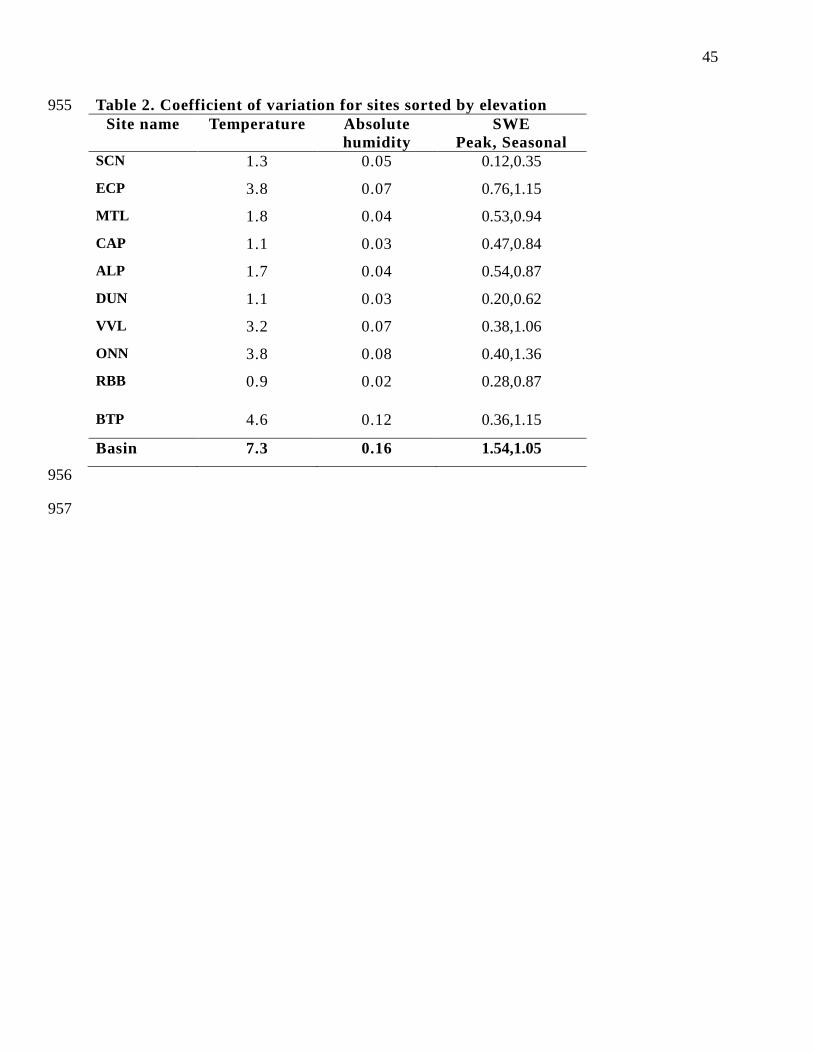
45

Table 2. Coefficient of variation for sites sorted by elevation 955 Site name Temperature Absolute

humidity SWE

Peak, Seasonal SCN 1.3 0.05 0.12,0.35

ECP 3.8 0.07 0.76,1.15

MTL 1.8 0.04 0.53,0.94

CAP 1.1 0.03 0.47,0.84

ALP 1.7 0.04 0.54,0.87

DUN 1.1 0.03 0.20,0.62

VVL 3.2 0.07 0.38,1.06

ONN 3.8 0.08 0.40,1.36

RBB 0.9 0.02 0.28,0.87

BTP 4.6 0.12 0.36,1.15

Basin 7.3 0.16 1.54,1.05

956

957

46

List of figures: 958

Figure 1 Location of American River basin and 14 sensor clusters deployed in the upper part of 959

the basin. 960

Figure 2 WSN nodes on hyposmetric curves with existing snow pillows 961

Figure 3. Node Layout and steady-state network connections (green lines) at Alpha, overlain on

Google Map. Sensor nodes are numbered. Two possible paths of data out from sensor node 5 to

the base station are marked with red arrows.

Figure 4. Average daily network performance of sensor nodes at Alpha for seven-month period.

Top panel shows number of network neighbors for each of the 10 sensor nodes, and bottom

panel is the average received signal strength indicator (RSSI) for each sensor node. A white gap

indicates no communication.

Figure 5. Scattered points of network packet delivery ratio (PDR) as a function of received

signal strength indicator (RSSI) from ten sensor nodes at Alpha

Figure 6. Measurements from the 10 nodes at Alpha over 2 weeks: a) hourly and daily mean air

temperature b) relative humidity, and c) snow depth.

Figure 7. Measurements from the 10 nodes at Bear Trap over a 3-day period: a) hourly mean air

temperature, b) relative humidity and c) absolute humidity. Data in black dashed line are from

met station within the footprint of the WSN cluster. The data from a nearby met-station are

marked as heavy dashed line.

Figure 8. Daily mean air temperature (Ta), and dew-point (Td) from sensor nodes at each WSN

cluster, along with temperature and precipitation data from nearby met stations. Shaded area

represent periods of precipitation.

47

Figure 9. Data from 10 clusters for 8-month period: a) daily average temperature, b) temperature

lapse rate, c) R2 value of daily lapse rate, d) mean (dashed lines) and standard deviation

(shading) of site air and dew-point temperatures adjusted to 2100 m elevation using the daily

lapse rate, e) daily average relative humidity, and f) daily vapor-pressure deficit calculated from

average daily temperature and relative humidity of each cluster.

Figure 10. Daily mean (µ) and standard deviation (σ) of SWE from the WSN clusters, plus

available operational snow-pillow data (red and green dashed), snow courses (yellow diamond)

and SNODAS SWE (blue dashed). Key to snow courses and snow pillows is on supplemental

information.

Figure 11. With dew-point temperature computed for each WSN clusters at hourly time step: a)

elevation of estimated of 0oC dew-point along with precipitation and SWE data from Echo Peak,

b) R2 value of the fit, c) RMSE of the fit in meters in elevation. The dashed blue lines indicate

the elevation range (minimum and maximum) of the WSN.

Figure 12. Snow deposition from five storms at WSN nodes within the 10 clusters. The increase

in SWE for each node and storm are plotted as scattered points in (a). Solid precipitation

adjusted to total precipitation with dew-point temperature in (b).

Figure 13. The elevational dependency of snow-free day. The mean (scattered points) and

standard deviation (horizontal bars) of the snowmelt progression for sensor nodes of each cluster

vs. elevation

962

48

963

Figure 3 Location of American River basin and 14 sensor clusters deployed in the upper part of 964

the basin. 965

966 967 968 969 970 971 972

973

Figure 4 WSN nodes on hyposmetric curves with existing snow pillows 974 975

49

976

Figure 3. Node Layout and steady-state network connections (green lines) at Alpha, overlain on

Google Map. Sensor nodes are numbered. Two possible paths of data out from sensor node 5 to

the base station are marked with red arrows. 977

978

979

Figure 4. Average daily network performance of sensor nodes at Alpha for seven-month period.

Top panel shows number of network neighbors for each of the 10 sensor nodes, and bottom

panel is the average received signal strength indicator (RSSI) for each sensor node. A white gap

indicates no communication.

50

980

981

Figure 5. Scattered points of network packet delivery ratio (PDR) as a function of received

signal strength indicator (RSSI) from ten sensor nodes at Alpha. 982

983

984

985

986

987

988

989

990

991

992

993

Figure 6. Measurements from the 10 nodes at Alpha over 2 weeks: a) hourly and daily mean air

temperature b) relative humidity, and c) snow depth. 994

51

995

Figure 7. Measurements from the 10 nodes at Bear Trap over a 3-day period: a) hourly mean air

temperature, b) relative humidity and c) absolute humidity. Data in black dashed line are from

met station within the footprint of the WSN cluster. The data from a nearby met-station are

marked as heavy dashed line.

996

52

997

998

Figure 8. Daily mean air temperature (Ta), and dew-point (Td) from sensor nodes at each WSN

cluster, along with temperature and precipitation data from nearby met stations. Shaded area

represent periods of precipitation.

53

999

Figure 9. Data from 10 clusters for 8-month period: a) daily average temperature, b) temperature

lapse rate, c) R2 value of daily lapse rate, d) mean (dashed lines) and standard deviation

(shading) of site air and dew-point temperatures adjusted to 2100 m elevation using the daily

lapse rate, e) daily average relative humidity, and f) daily vapor-pressure deficit calculated from

average daily temperature and relative humidity of each cluster.

1000

54

1001

55

Figure 10. Daily mean (µ) and standard deviation (σ) of SWE from the WSN clusters, plus

available operational snow-pillow data (red and green dashed), snow courses (yellow diamond)

and SNODAS SWE (blue dashed). Key to snow courses and snow pillows is on supplemental

information.

1002

1003

Figure 11. With dew-point temperature computed for each WSN clusters at hourly time step: a)

elevation of estimated of 0oC dew-point along with precipitation and SWE data from Echo Peak,

b) R2 value of the fit, c) RMSE of the fit in meters in elevation. The dashed blue lines indicate

the elevation range (minimum and maximum) of the WSN. 1004

56

1005

Figure 12. Snow deposition from five storms at WSN nodes within the 10 clusters. The increase

in SWE for each node and storm are plotted as scattered points in (a). Solid precipitation

adjusted to total precipitation with dew-point temperature in (b).

1006

1007

Figure 13. the elevational dependency of snow-free day. The mean (scattered points) and

standard deviation (horizontal bars) of the snowmelt progression for sensor nodes of each cluster

vs. elevation.