Embed Size (px)
Citation preview

Page 1 of 54
Technical report: the design and evaluation of a basin-scale wireless sensor network for mountain hydrology
Ziran Zhang1, Steven D. Glaser1, Roger C. Bales1,2, Martha Conklin2, Robert Rice2 and
Danny G. Marks3
1Department of Civil and Environmental Engineering, University of California, Berkeley,
Berkeley, USA. 2Sierra Nevada Research Institute and School of Engineering, University of California, Merced,
Merced, USA. 3Agricultural Research Service, USDA, Boise, USA.
Ziran Zhang ([email protected])
Steven Glaser ([email protected])
Roger Bales ([email protected])
Martha Conklin ([email protected])
Robert Rice ([email protected])
Danny Marks ([email protected])
Key Points:
– This first basin-scale wireless-sensor network provides reliable, representative measurements in a mountain basin.
– The distributed network better characterizes patterns of key hydrologic variables compared to operational networks
– Used with spatially explicit modeling and other spatial data, the network offers unprecedented opportunities for improved hydrologic prediction

Page 1 of 54
Abstract 1
A network of sensors for spatially representative water-balance measurements was developed 2
and deployed across the 2000 km2 snow-dominated portion of the upper American River basin, 3
primarily to measure changes in snowpack and soil-water storage, air temperature and humidity. 4
This wireless sensor network (WSN) consists of 14 sensor clusters, each with 10 measurement 5
nodes that were strategically placed within a 1-km2 area, across different elevations, aspects, 6
slopes and canopy covers. Compared to existing operational sensor installations, the WSN 7
reduces hydrologic uncertainty in at least three ways. First, redundant measurements improved 8
estimation of lapse rates for air and dew-point temperature. Second, distributed measurements 9
captured local variability and constrained uncertainty in air and dew-point temperature, snow 10
accumulation and derived hydrologic attributes important for modeling and prediction. Third, 11
the distributed relative-humidity measurements offer a unique capability to monitor upper-basin 12
patterns in dew-point temperature and characterize elevation gradient of water vapor-pressure 13
deficit across steep, variable topography. Network statistics during the first year of operation 14
demonstrated that the WSN was robust for cold, wet and windy conditions in the basin. The 15
electronic technology used in the WSN reduced adverse effects, such as high current 16
consumption, multipath signal fading and clock drift, seen in previous remote WSNs. 17
18
Index Terms and Keywords: 19
Wireless-sensor network, water-information system, snow observation, mountain 20
hydrology, Sierra Nevada. 21

Page 2 of 54
1 Introduction 22
Currently, in situ measurements of mountain water cycles at the basin scale are limited in 23
both spatial coverage and temporal resolution, with data largely provided by a relatively small 24
number of operational precipitation, snowpack, climate and stream-gauging stations [Bales et al., 25
2006; Dozier, 2011]. In the Sierra Nevada, measurement sites supporting operational water-26
resources decision making are also biased to middle and lower elevations and flat terrain in 27
forest clearings [Molotch and Bales, 2005]. 28
Hydrologic prediction, particularly when constrained by the practical demands of water-29
resources management, relies heavily on calibrated models to mitigate both limitations in model 30
formulation and inadequate data for rigorous model testing [Kuczera et al., 2010; Semenova and 31
Beven, 2015]. There are increasing demands on distributed models as predictive tools for 32
situations in which lumped models may fall short, such as non-stationarity in catchment 33
conditions or climate; however, their use in water-resources management is limited by the level 34
of field data available [Refsgaard, 1997]. The need for improved coverage by in situ 35
measurements is both local and global, and new network designs should complement satellite 36
data [Wood et al., 2011]. Ground-based sensors provide critical ground truth for remotely sensed 37
satellite and aircraft data, and offer a wide suite of independent data that can help provide much-38
needed gains in predictive modeling. Realizing gains in accuracy from the next generation of 39
spatially explicit models at the scale of water-resources decision making will require both the 40
broad spatial coverage of remotely sensed data and the accuracy of in situ measurements 41
[Lehning et al., 2009]. An adaptive rather than one-size-fits-all approach is needed to realize 42
these gains [Fenicia et al., 2008]. 43

Page 3 of 54
Wireless Sensor Networks (WSNs) are an efficient and economical solution for 44
distributed sensing. It is often costly and disruptive to create networks of spatially 45
representative wired sensors at the scale desired since it might require kilometers of cables 46
placed either above ground or buried. Similarly, access to data for distributed sensors with only 47
local logging is limited by the need to visit sites to download data. Reliable wireless solutions 48
are now enabled by reduced production costs of wireless equipment and by advances in 49
networking protocols, effectively combining traditionally wired sensors with a wireless 50
platform. [Akyildiz et al., 2002; Yick et al., 2008; Gilbert, 2012]. 51
A few WSN solutions, using different network technologies, were developed specifically 52
for applications in hydrology. These studies have not provided quantifiable assessments of 53
network design, operation and hydrologic results at the river-basin scale. A review of these prior 54
deployments, and a comparison of three existing WSN solutions that have been used, is provided 55
in supporting information (See text S1) [Digi, n.d.; Bogena et al., 2010; Pister and Doherty, 56
2008; Gungor and Hancke, 2009; International, 2009; Ritsema et al., 2010; Simoni et al., 2011; 57
Horvat, 2012; Huang et al., 2012; Kerkez et al., 2012; Accettura and Piro, 2014; Pohl et al., 58
2014; ZigBee, 2009]. 59
While sensor networks deployed in headwater catchments for short durations offer 60
lessons for local-scale WSNs, they provide limited guidance for WSN design, performance and 61
hydrologic benefits for systems in larger mountain river basins, characterized by steep gradients 62
in temperature, precipitation, rain-versus-snow fraction, growing season, vegetation density and 63
evapotranspiration. The proposed approach to scaling WSN measurements to larger basins 64
involves strategically placing local clusters to capture the variability in hydrologically important 65
basin attributes [Welch et al., 2013]. 66

Page 4 of 54
The aim of the research described in this technical report was to develop a flexible, robust 67
method for measurement of the spatial water balance across a seasonally snow-covered mountain 68
basin. In doing this, we addressed three questions. First, to what extent can a basin-scale 69
distributed wireless-sensor network with a limited number of sensors arrayed in local clusters 70
sample hydrologic variables across a representative range of landscape attributes in a seasonally 71
snow-covered mountain basin? Second, to what extent can this low-power, distributed wireless-72
sensor network reliably provides hydrologic data during harsh winter conditions? Third, what 73
types of gains in hydrologic information may result from this network? Further development and 74
more-detailed analysis of the third question is also the subject of subsequent analysis. 75
2 Methods 76
The network was deployed in the American River Hydrologic Observatory (ARHO), in 77
the upper, snow-dominated portion of the American River basin on the western slope of the 78
Sierra Nevada in California (36.069 N, -120.583 W). The basin is incised with steep river 79
canyons and is comprised of three sub-basins: the North, Middle, and South forks, which 80
combine to form a drainage basin of 5311 km2 above the Folsom Reservoir, the main 81
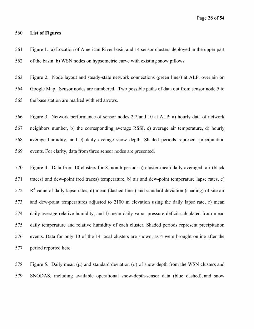
impoundment on the river (Fig. 1a). Basin elevations range from 15 m at Folsom to 3147 m at 82
the Sierra crest, with precipitation transitioning from rain to snow at about 1400-1600 m 83
elevation [Raleigh and Lundquist, 2012; Klos et al., 2014]. Forty percent, or about 2000 km2, 84
of the basin is above 1500 m, the lowest elevation for siting our WSNs. About 0.5% of the 85
basin is above the highest node that was sited (2678 m). 86
In 2013-2015, 14 clusters of wireless nodes were deployed (Fig. 1a), with locations 87
selected to represent the range of elevation, aspect, canopy coverage, and solar loading in the 88
basin (Fig. 1b and S1). Each node had a number of sensors, as described in Supporting 89

Page 5 of 54
Information; with air temperature, relative humidity and snow depth the subject of this report. 90
The number of local clusters was based on results of Welch et al. [2013], and constrained by 91
project budget. The Welch et al. analysis used spatial time-series data over 11 years and a rank-92
based clustering approach to identify measurement locations that will be most informative for 93
real-time estimation of snow depth, and derived a set of regions that remained relatively stable 94
over time. They found a point of marginal return at about 15 measurement locations, after which 95
placing more local sensor networks did not significantly improve estimation performance. The 96
Welch et al. study also showed that there is some flexibility in placing the local clusters to 97
capture representative parts of the basin, and thus all sites, except MTL and DOR, were co-98
located with existing snow pillows and met stations. Each cluster consists of ten measurement 99
nodes, limited due to budget, seven to 35 signal-repeater nodes, and a network manager (see 100
Table S1 for details; and Fig. S2 for system hierarchy). 101
Measurement-node placement consisted of three steps. First, major physiographic 102
variables that affect snow distribution, and by extension other components of the water balance, 103
were characterized in a 1-km2 area around each site [Balk and Elder, 2000; Erxleben et al., 2002; 104
Anderton et al., 2004; Essery and Pomeroy, 2004; Sturm and Benson, 2004; Erickson et al., 2005; 105
Marchand and Killingtveit, 2005; Bales et al., 2006]. Second, at each site ten points representing 106
different physiographic attributes were selected by a random-stratified technique, and the 107
attributes aggregated to assess their representativeness in the larger basin (See text S2 [Jin et al., 108
2013]). Rice and Bales [2010] showed that a 10-sensor network could capture the mean and 109
distribution of snow depths at this scale. Third, final location adjustments were made in the field 110
to a small subset of sensor nodes, ensuring a complete sampling of the physiographic features 111
Page 6 of 54
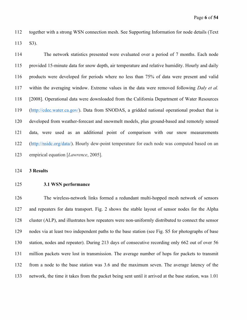
together with a strong WSN connection mesh. See Supporting Information for node details (Text 112
S3). 113
The network statistics presented were evaluated over a period of 7 months. Each node 114
provided 15-minute data for snow depth, air temperature and relative humidity. Hourly and daily 115
products were developed for periods where no less than 75% of data were present and valid 116
within the averaging window. Extreme values in the data were removed following Daly et al. 117
[2008]. Operational data were downloaded from the California Department of Water Resources 118
(http://cdec.water.ca.gov/). Data from SNODAS, a gridded national operational product that is 119
developed from weather-forecast and snowmelt models, plus ground-based and remotely sensed 120
data, were used as an additional point of comparison with our snow measurements 121
(http://nsidc.org/data/). Hourly dew-point temperature for each node was computed based on an 122
empirical equation [Lawrence, 2005]. 123
3 Results 124
3.1 WSN performance 125
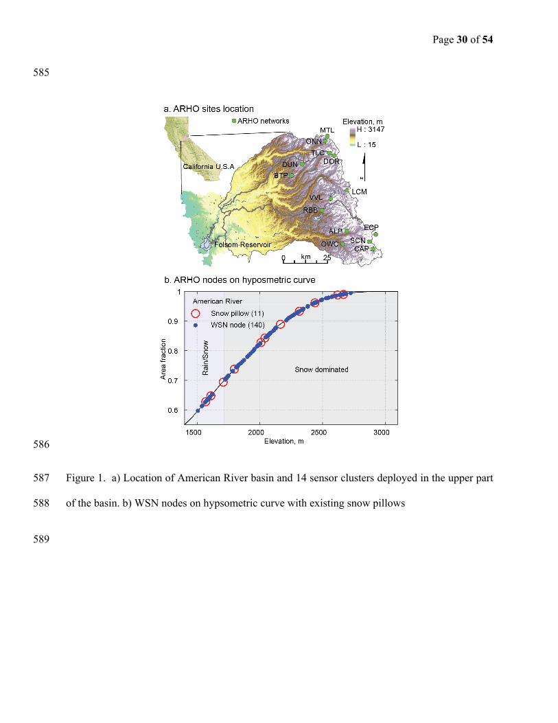
The wireless-network links formed a redundant multi-hopped mesh network of sensors 126
and repeaters for data transport. Fig. 2 shows the stable layout of sensor nodes for the Alpha 127
cluster (ALP), and illustrates how repeaters were non-uniformly distributed to connect the sensor 128
nodes via at least two independent paths to the base station (see Fig. S5 for photographs of base 129
station, nodes and repeater). During 213 days of consecutive recording only 662 out of over 56 130
million packets were lost in transmission. The average number of hops for packets to transmit 131
from a node to the base station was 3.6 and the maximum seven. The average latency of the 132
network, the time it takes from the packet being sent until it arrived at the base station, was 1.01 133
Page 7 of 54
second. On average, each node received 181,000 packets over the period when network statistics 134
were gathered. 135
Two measures indicate the reliability and performance of the network: i) the number of 136
other sensor or repeater nodes connected to each node and ii) the average received signal 137
strength indicator (RSSI). RSSI is closely associated with an important network-performance 138
indicator called packet delivery ratio (PDR). In aggregate, each node was connected to at least 139
two other nodes over 95% of the time, and to three or more nodes 68% of the time (see Fig. S6). 140
Taking all nodes together, RSSI values were above -85 dBm, the manufacturer-specified 141
threshold for efficient transmission over 54% of the time, with values above -80 dBm 33% of 142
the time. 143
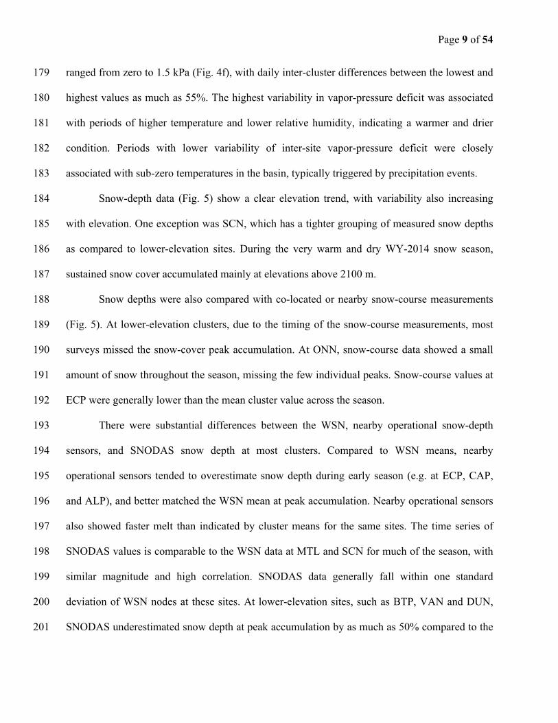
Environmental factors have been thought to impact the performance of WSNs [Boano et 144
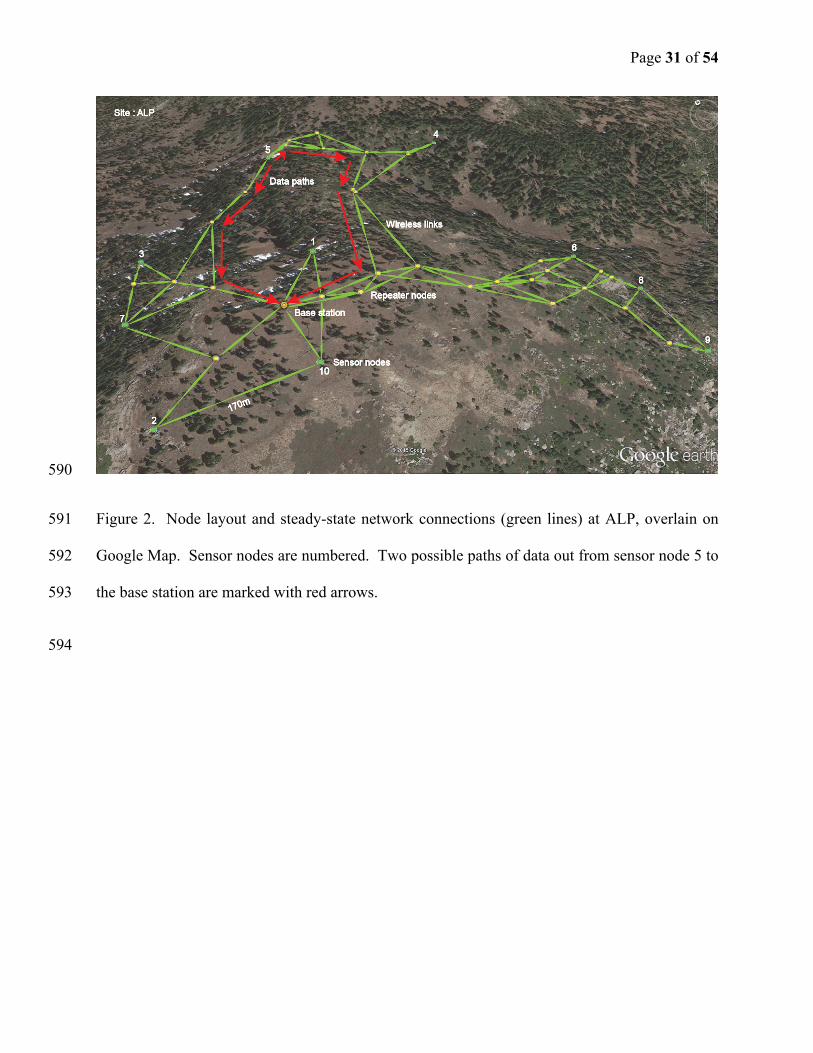
al., 2010; Marfievici et al., 2013]. For our local clusters there was no clear influence of 145
environmental factors, e.g., temperature, humidity and snow-induced topographic changes, on 146
network performance (Fig. 3). Each node was connected to one to five other nodes at each time 147
step (Fig. 3a). RSSI values at each node typically fluctuated +5 dBm, and the average RSSI (Fig. 148
3b) depended on node location as opposed to temperature (Fig. 3c), humidity (Fig. 3d) or 149
topographic changes due to snow accumulation (see water-year days 72 and 80, Fig. 3e). It was 150
discovered that absolute topography influenced connectivity. 151
3.2 Temperature, humidity and snow patterns 152
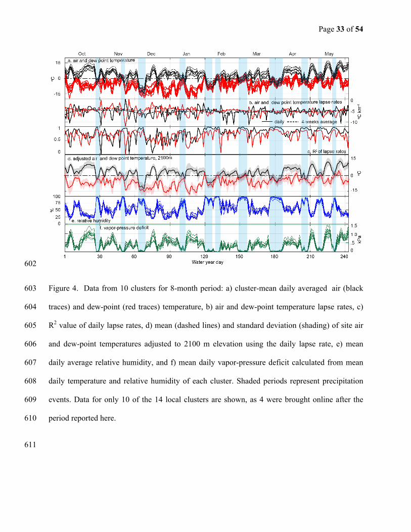
Daily air and dew-point temperatures from the 10 wireless-sensor clusters that were 153
installed prior to the 2014 water year showed very similar temporal patterns (Fig. 4a), with 154
average temperature differences reflecting elevation differences between clusters. Temperatures 155
Page 8 of 54
for all pairs of clusters were highly correlated, r > 0.91 for air temperature and r >0.86 for dew-156
point temperature, p < 0.05. 157
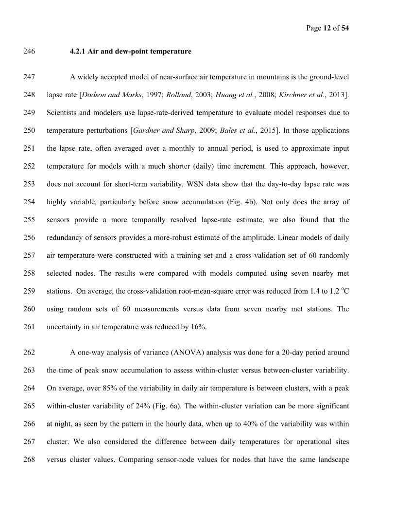
Daily temperatures were used to derive surface-level lapse rates, which over the eight-158
month period varied from close to zero to -12oC/km for both air and dew-point temperatures (Fig. 159
4b). The respective average lapse rates for the months before snow accumulation (Oct-Dec) were 160
-4.6 and -5.7 oC/km, increasing to -5.5 oC/km for air temperature and decreasing to -4.7 oC/km 161
for dew-point temperature during the snow season. The day-to-day variability in lapse rates 162
during the snow-covered period was also lower than earlier in the water year. The transition to a 163
period with less variability in lapse rate is also illustrated by the higher R2 values starting on 164
water-year day 121, when snow started accumulating in the basin (Fig 4c). Note that less-165
negative air-temperature lapse rates, associated with lower R2 values, were associated with 166
temperature inversions. 167
Daily mean air and dew-point temperatures taken across the ten clusters were adjusted to 168
2100 m using the mean daily lapse rates (Fig. 4d). The average standard deviation is 3.3 oC for 169
air temperature and 3.5 oC for dew-point temperature, a variability equivalent to the average 170
difference over about 600 m and 545 m elevation based on the eight-month average lapse rate of 171
-5.5 oC/km and -5.0 oC/km, respectively. While any index elevation could be used for this 172
comparison, 2100 m is generally representative of the upper part of the rain-snow-transition 173
elevation zone. 174
Mean relative humidity across WSN clusters varied from 15 to 100%, with similar 175
patterns across all 10 clusters (Fig. 4e). The correlations were strong, r = 0.91, p < 0.05, for all 176
pairs of clusters. Differences in absolute humidity and vapor-pressure deficit between clusters 177
were in some cases relatively large. The mean water vapor-pressure deficit for each cluster 178
Page 9 of 54
ranged from zero to 1.5 kPa (Fig. 4f), with daily inter-cluster differences between the lowest and 179
highest values as much as 55%. The highest variability in vapor-pressure deficit was associated 180
with periods of higher temperature and lower relative humidity, indicating a warmer and drier 181
condition. Periods with lower variability of inter-site vapor-pressure deficit were closely 182
associated with sub-zero temperatures in the basin, typically triggered by precipitation events. 183
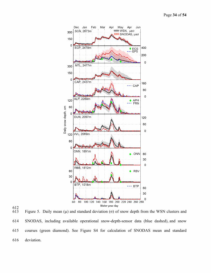
Snow-depth data (Fig. 5) show a clear elevation trend, with variability also increasing 184
with elevation. One exception was SCN, which has a tighter grouping of measured snow depths 185
as compared to lower-elevation sites. During the very warm and dry WY-2014 snow season, 186
sustained snow cover accumulated mainly at elevations above 2100 m. 187
Snow depths were also compared with co-located or nearby snow-course measurements 188
(Fig. 5). At lower-elevation clusters, due to the timing of the snow-course measurements, most 189
surveys missed the snow-cover peak accumulation. At ONN, snow-course data showed a small 190
amount of snow throughout the season, missing the few individual peaks. Snow-course values at 191
ECP were generally lower than the mean cluster value across the season. 192
There were substantial differences between the WSN, nearby operational snow-depth 193
sensors, and SNODAS snow depth at most clusters. Compared to WSN means, nearby 194
operational sensors tended to overestimate snow depth during early season (e.g. at ECP, CAP, 195
and ALP), and better matched the WSN mean at peak accumulation. Nearby operational sensors 196
also showed faster melt than indicated by cluster means for the same sites. The time series of 197
SNODAS values is comparable to the WSN data at MTL and SCN for much of the season, with 198
similar magnitude and high correlation. SNODAS data generally fall within one standard 199
deviation of WSN nodes at these sites. At lower-elevation sites, such as BTP, VAN and DUN, 200
SNODAS underestimated snow depth at peak accumulation by as much as 50% compared to the 201

Page 10 of 54
WSN. At all other sites, SNODAS overestimated peak-accumulation snow depth by as much as 202
80% compared to the WSN mean. 203
4 Discussion 204
4.1 WSN design and performance 205
With 555 sensors across 14 clusters, the WSN offers representative, real-time monitoring 206
of the meteorological and hydrologic conditions of much of the upper reaches of the basin. The 207
size of this network, arguably the largest long-term, remote wireless-sensor platform deployed 208
for environmental monitoring, shows that WSNs are now capable of being used for major 209
instrumentation projects. Even though some aspects of the networks in ARHO share similar 210
properties with the prototype installation at the Southern California Critical Zone Observatory 211
[Kerkez et. al. 2012], the more-recent network statistics help to resolve several previously 212
unanswered networking questions important to the broader wireless communications community 213
as well as to field hydrologists. The longer-term performance of the networks, subjected to the 214
test of a full snow season, showed that WSNs can be a viable solution for distributed sensing at 215
this scale. ARHO networks showed resilience to factors such as humidity and snow-induced 216
topographic changes across different part of the basin. The positive result is likely due to the 217
combination of the Dust Network’s radio technologies such as time-synchronized channel-218
hopping, time-slotted mesh protocol (see section S1.2.3 for details of the technology), effective 219
network topology, and the use of lower-gain antennas. 220
A stringent criterion of design was low power consumption, requiring the sensor node to 221
be powered with a 6-amp-hour battery recharged by a 10-watt solar panel. The low-power 222
requirement constrains radio-power output, so the range of the radio limits the size and 223

Page 11 of 54
performance of the network. Through iterative design and careful control over circuitry we were 224
able to attain our goal. The final design is basically two very low-power-consumption microchips 225
– a Cypress PSoC5 and Dust networks radio module. This is useful to the community, which by 226
and large uses systems based on technology that has 100 or more times the power consumption 227
(see Supporting Information). 228
Topographic relief is one of the more-serious challenges to overcome for good system 229
performance. Different from earlier installations, the networks in ARHO encountered more-230
challenging, steep forested terrain. A lower-gain 4-dBm gain omni-directional antenna provided 231
improved network connectivity due to its “fatter” radiation pattern, especially in steep terrain, 232
compared to the 12-dBm gain antennas used by Kerkez et al [2012] on more-even terrain. Even 233
with the improvement, the capability of the network to communicate over steep slopes is limited 234
by the antenna. The ALP site is a good example of where some radio links operated at the edge 235
of the acceptable RSSI level due to steep topography. A relatively large number of repeaters 236
were installed to provide redundant paths to sensor nodes 6, 8, and 9, where a steep change in 237
slope produced a radio path “kink” and reliable network links were challenging to establish. The 238
network performance was stable but less efficient, indicated by the lower PDR values, compared 239
to Kerkez et al. [2012], who had shorter data hops. 240
4.2 Spatial pattern and variability of hydrologic attributes 241
The following three examples illustrate how our spatially distributed, daily data over 242
complex terrain set provides improved estimates of important hydrologic attributes, compared to 243
less-dense operational measurements. A more-detailed analysis will be the subject of a 244
subsequent report. 245
Page 12 of 54
4.2.1 Air and dew-point temperature 246
A widely accepted model of near-surface air temperature in mountains is the ground-level 247
lapse rate [Dodson and Marks, 1997; Rolland, 2003; Huang et al., 2008; Kirchner et al., 2013]. 248
Scientists and modelers use lapse-rate-derived temperature to evaluate model responses due to 249
temperature perturbations [Gardner and Sharp, 2009; Bales et al., 2015]. In those applications 250
the lapse rate, often averaged over a monthly to annual period, is used to approximate input 251
temperature for models with a much shorter (daily) time increment. This approach, however, 252
does not account for short-term variability. WSN data show that the day-to-day lapse rate was 253
highly variable, particularly before snow accumulation (Fig. 4b). Not only does the array of 254
sensors provide a more temporally resolved lapse-rate estimate, we also found that the 255
redundancy of sensors provides a more-robust estimate of the amplitude. Linear models of daily 256
air temperature were constructed with a training set and a cross-validation set of 60 randomly 257
selected nodes. The results were compared with models computed using seven nearby met 258
stations. On average, the cross-validation root-mean-square error was reduced from 1.4 to 1.2 oC 259
using random sets of 60 measurements versus data from seven nearby met stations. The 260
uncertainty in air temperature was reduced by 16%. 261
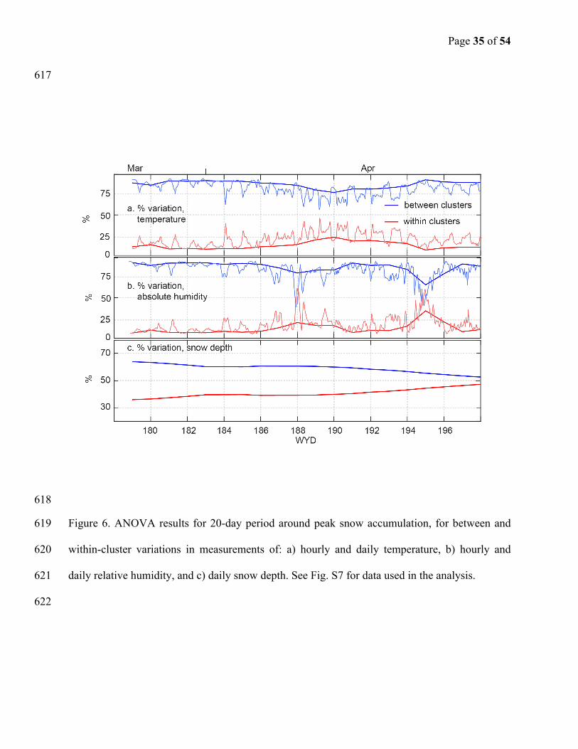
A one-way analysis of variance (ANOVA) analysis was done for a 20-day period around 262
the time of peak snow accumulation to assess within-cluster versus between-cluster variability. 263
On average, over 85% of the variability in daily air temperature is between clusters, with a peak 264
within-cluster variability of 24% (Fig. 6a). The within-cluster variation can be more significant 265
at night, as seen by the pattern in the hourly data, when up to 40% of the variability was within 266
cluster. We also considered the difference between daily temperatures for operational sites 267
versus cluster values. Comparing sensor-node values for nodes that have the same landscape 268
Page 13 of 54
features as do operational measurements (flat, open) versus other nodes shows a 0.8oC difference 269
for one site, and 0-0.3oC for five other sites; however the values are not different at the 95% 270
confidence level (Figure S8a). 271
Dew-point temperature complements air temperature in providing a reliable estimate of 272
the timing and phase of precipitation. The reduction of uncertainty in temperature and humidity 273
patterns helps to better determine the elevation range of the rain/snow transition. Air temperature 274
is approximately equal to dew-point temperature, indicating saturated air, when precipitation 275
occurs (Fig. 4). The phase change from rain to snow usually occurs around the 0oC dew-point 276
[Marks et al., 2013]. Compared to air-temperature-based methods, dew-point temperature is a 277
less geographically dependent variable to determine the solid or liquid precipitation [Ye et al., 278
2013]. Due to lack of relative-humidity measurements for most met stations, calculation of dew-279
point temperature cannot be performed from met-station data alone. 280
Feld et al. [2013] assessed various methods of estimating daily dew point, and found that 281
a weather-forecast model that captured some aspects of local topography provided less-biased 282
estimates than did simpler constant-lapse-rate or constant-humidity approaches. Their median 283
dew-point lapse rate, based on 15 met stations and 35 hygrochons deployed in the North Fork 284
American basin and averaged over 3 years, was -5.3 oC/km, comparable to our mean of -5.0 285
oC/km. However, our -5.5 oC/km mean air-temperature lapse rate was smaller than their 3-year 286
average of -6.3 oC/km. More extensive analysis of our seasonal and spatial patterns will be the 287
subject of a subsequent report. 288
4.2.2. Evaporative potential 289
Page 14 of 54
Direct measures of vapor-pressure-deficit patterns from a dense array of ground-based 290
sensors can be important for scaling evapotranspiration and assessing forest health [Oren et al., 291
1999, 2001; Bowling et al., 2002]. Accurately estimating vapor-pressure deficit is crucial as the 292
saturation-pressure deficit becomes relatively more important in the Penman-Monteith equation 293
[Ziemer, 1979]. Despite the importance of the variable, reliable field-based estimates of vapor-294
pressure deficit in mountains are rare. The performance of satellite-based estimates varies, with 295
RMSE values from upwards of 0.3 kPa to 1.1 kPa, limiting their accuracy as estimates of vapor-296
pressure deficit across steep terrain [Prince et al., 1998; Hashimoto et al., 2008]. A WSN with 297
relative-humidity measurement at every sensor node fills this gap. 298
The ANOVA results for daily relative humidity are similar to those for temperature, with 299
most of the variance being between versus within clusters (Fig. 6b). There was, however, no 300
clear day-night pattern. In addition, there were only small differences in humidity between nodes 301
that represent the varying landscape attributes of operational sensors, versus values for other 302
nodes. One of the 6 sites evaluated had a significant difference, reflecting in large part the 303
temperature differences (Figure S8b). 304
4.2.3 Snow depth 305
The differences in snow depth between WSN and nearby operational sensors can be 306
explained by the patterns of snow accumulation. Operational snow-depth sensors are typically 307
placed near flat meadows or ridge tops free of overhead obstructions or hazards, which produce 308
known biases [Molotch and Bales, 2006; Ainslie and Jackson, 2010; Rice and Bales, 2010]. We 309
placed our nodes in both forested and non-forested area to produce a more spatially 310
representative measurement. Fig. 5 indicates that operational snow-depth sensors data had a 311
systematic positive bias in snow depth in the early season. During the melting season, the canopy 312
Page 15 of 54
acts as a shield, limiting energy input to the snowpack [Marks et al., 1998; Sicart et al., 2004; 313
Pomeroy et al., 2012]. The canopy also shelters the snow surface from wind, reducing turbulent 314
heat transfer. The net result is an extended melt season recorded by sensor nodes in the forested 315
area compared to the operational snow-depth sensors. 316
The ANOVA results for daily snow depth show that both within-cluster and between-317
cluster variability to be important. About 60% of the variability was between clusters and 40% 318
within clusters immediately after the accumulation event ending on water-year day 183, with 319
both values converging toward 50% over the next 2 weeks. Comparing nodes having landscape 320
attributes like those of operational sites (flat, open) versus other nodes also shows relatively large 321
within-cluster differences between the two sets at most of the six sites evaluated (Figure S8c). 322
Due to local redundancy of the WSN, the data stream is more complete than operational 323
snow-depth sensors at CAP and BTP. Large sections of data were missing from the operational-324
snow-depth sensors from those two sites during the storm around water-year day 180 (Fig. 5). 325
This reflects a reality of operational water-resources networks, namely the inability to respond in 326
a timely manner to problems in remote sensors. The redundancy provided by our WSNs helps to 327
address this constraint. 328
The differences in snow depth between SNODAS and the WSN were less systematic, as 329
there is no apparent trend in the bias across different sites. One pronounced difference between 330
WSN and SNODAS snow depth was at the steep ECP site, where the 1-km2 SNODAS product 331
overestimated snow depth compared to our measurements (Fig. 5). This follows previous reports 332
that without sufficient data, estimates of snow depth under these conditions can be difficult and 333
error prone due to the underlying variance in elevation within grid boundaries [Hedrick et al., 334
2015]. Clow et al. [2012] showed that for over-forested regions of the Colorado Rockies, 335
Page 16 of 54
SNODAS estimates of snow depth accounted for as much as 72% of the variance line (1-km 336
resolution) in forested areas, but SNODAS was only able to account for 16% of snow-depth 337
variance in areas above the treeline. 338
5 Conclusions 339
A wireless-sensor network distributed over the 2000 km2 snow-dominated portion of a 340
mountain basin provided effective coverage of watershed attributes. With ten measurement 341
nodes per each of fourteen clusters, the WSNs reliably provided spatially distributed 342
measurements of temperature, relative humidity and snow depth every 15 minutes over the basin. 343
The WSN also provided measurements of the significant within-cluster spatial variability of 344
these attributes, which were influenced by local topography, possibly through cold-air drainage 345
effects on temperature. 346
Compared to existing operational sensors, the wireless-sensor network reduces 347
uncertainty in water-balance measurements in at least three distinct ways. Redundant 348
measurements in temperature improved the robustness of temperature lapse-rate estimation, 349
reducing cross-validation error compared to that of using met-station data alone. Second, 350
distributed measurements capture local variability and constrain uncertainty, compared to point 351
measures, in attributes important for hydrologic modeling, such as air and dew-point temperature 352
and snow precipitation. Third, the distributed relative-humidity measurements offer a unique 353
capability to monitor upper-basin patterns in dew-point temperature and better characterize 354
precipitation phase and the elevation of the rain/snow transition. 355
Acknowledgments 356
The work presented in this paper is supported by the National Science Foundation (NSF) 357
through a Major Research Instrumentation Grant (EAR-1126887), the Sierra Nevada Research 358

Page 17 of 54
Institute, the Southern Sierra Critical Zone Observatory (EAR-0725097), California Department 359
of Water Resources (Task Order UC10-3), the UC Water Security and Sustainability Research 360
Initiative and USDA-ARS CRIS Snow and Hydrologic Processes in the Intermountain West 361
(5362-13610-008-00D). Data used to support the analysis can be obtained upon request from the 362
authors. 363
364
Page 18 of 54
References 365
Accettura, N., and G. Piro (2014), Optimal and secure protocols in the IETF 6TiSCH 366
communication stack, Proc. IEEE Int. Symp. Ind. Electron., 367
doi:10.1109/ISIE.2014.6864831. 368
Accettura, N., and G. Piro (2014), Optimal and Secure Protocols in the IETF 6TiSCH 369
communication stack, Proc. IEEE Int. Symp. Ind. Electron., 370
doi:10.1109/ISIE.2014.6864831. 371
Ainslie, B., and P. L. Jackson (2010), Downscaling and bias correcting a cold season 372
precipitation climatology over coastal southern British Columbia using the regional 373
atmospheric modeling system (RAMS), J. Appl. Meteorol. Climatol., 49(5), 937–953, 374
doi:10.1175/2010JAMC2315.1. 375
Akyildiz, I., W. Su, Y. Sankarasubramaniam, and E. Cayirci (2002), Wireless sensor networks: a 376
survey, Comput. Networks, 38(4), 393–422, doi:10.1016/S1389-1286(01)00302-4. 377
Anderton, S. P., S. M. White, and B. Alvera (2004), Evaluation of spatial variability in snow 378
water equivalent for a high mountain catchment, Hydrol. Process., 18(3), 435–453, 379
doi:10.1002/hyp.1319. 380
Bales, R. C., N. P. Molotch, T. H. Painter, M. D. Dettinger, R. Rice, and J. Dozier (2006), 381
Mountain hydrology of the western United States, Water Resour. Res., 42(8), 1–13, 382
doi:10.1029/2005WR004387. 383
Page 19 of 54
Bales, R. C., R. Rice, and S. B. Roy (2015), Estimated loss of snowpack storage in the Eastern 384
Sierra Nevada with climate warming, J. Water Resour. Plan. Manag., 141(2), 4014055, 385
doi:10.1061/(ASCE)WR.1943-5452.0000453. 386
Balk, B., and K. Elder (2000), Combining binary decision tree and geostatistical methods to 387
estimate snow distribution in a mountain watershed, Water Resour. Res., 36(1), 13–26, 388
doi:10.1029/1999WR900251. 389
Boano, C. A., N. Tsiftes, T. Voigt, J. Brown, and U. Roedig (2010), The impact of temperature 390
on outdoor industrial sensornet applications, IEEE Trans. Ind. Informatics, 6(3), 451–459, 391
doi:10.1109/TII.2009.2035111. 392
Bogena, H. R., J. a. Huisman, C. Oberdörster, and H. Vereecken (2007), Evaluation of a low-cost 393
soil water content sensor for wireless network applications, J. Hydrol., 344(1–2), 32–42, 394
doi:10.1016/j.jhydrol.2007.06.032. 395
Bogena, H. R., M. Herbst, J. a. Huisman, U. Rosenbaum, a. Weuthen, and H. Vereecken (2010), 396
Potential of wireless sensor networks for measuring soil water content variability, Vadose 397
Zo. J., 9(4), 1002, doi:10.2136/vzj2009.0173. 398
Bowling, D. R., N. G. McDowell, B. J. Bond, B. E. Law, and J. R. Ehleringer (2002), 13C 399
content of ecosystem respiration is linked to precipitation and vapor pressure deficit, 400
Oecologia, 131(1), 113–124, doi:10.1007/s00442-001-0851-y. 401
Clow, D. W., L. Nanus, K. L. Verdin, and J. Schmidt (2012), Evaluation of SNODAS snow 402
depth and snow water equivalent estimates for the Colorado Rocky Mountains, USA, 403
Hydrol. Process., 26(17), 2583–2591, doi:10.1002/hyp.9385. 404

Page 20 of 54
Daly, C., M. Halbleib, J. I. Smith, W. P. Gibson, M. K. Doggett, G. H. Taylor, and P. P. Pasteris 405
(2008), Physiographically sensitive mapping of climatological temperature and precipitation 406
across the conterminous United States, doi:10.1002/joc. 407
Digi, Digi International (n.d.), XBee/XBee-PRO DigiMesh 2.4 user guide. 408
Document, Z. (2009), ZigBee RF4CE : ZRC Profile Specification. 409
Dodson, R., and D. Marks (1997), Daily air temperature interpolated at high spatial resolution 410
over a large mountainous region, Clim. Res., 8(1), 1–20, doi:10.3354/cr008001. 411
Dozier, J. (2011), Mountain hydrology, snow color, and the fourth paradigm, Eos (Washington. 412
DC)., 92(43), 373–374, doi:10.1029/2011EO430001. 413
Erickson, T. a., M. W. Williams, and A. Winstral (2005), Persistence of topographic controls on 414
the spatial distribution of snow in rugged mountain terrain, Colorado, United States, Water 415
Resour. Res., 41(4), 1–17, doi:10.1029/2003WR002973. 416
Erxleben, J., K. Elder, and R. Davis (2002), Comparison of spatial interpolation methods for 417
estimating snow distribution in the Colorado Rocky Mountains, Hydrol. Process., 16(18), 418
3627–3649, doi:10.1002/hyp.1239. 419
Essery, R., and J. Pomeroy (2004), Vegetation and topographic control of wind-blown snow 420
distributions in distributed and aggregated simulations for an arctic tundra basin, J. 421
Hydrometeorol., 5(5), 735–744, doi:10.1175/1525-422
7541(2004)005<0735:VATCOW>2.0.CO;2. 423
Page 21 of 54
Feld, S. I., N. C. Cristea, and J. D. Lundquist (2013), Representing atmospheric moisture content 424
along mountain slopes: Examination using distributed sensors in the Sierra Nevada, 425
California, Water Resour. Res., 49(7), 4424–4441, doi:10.1002/wrcr.20318. 426
Fenicia, F., J. J. McDonnell, and H. H. G. Savenije (2008), Learning from model improvement: 427
On the contribution of complementary data to process understanding, Water Resour. Res., 428
44(6), doi:10.1029/2007WR006386. 429
Gardner, A., and M. Sharp (2009), Sensitivity of net mass-balance estimates to near-surface 430
temperature lapse rates when employing the degree-day method to estimate glacier melt, 431
Ann. Glaciol., 50(1), 80–86, doi:10.3189/172756409787769663. 432
Gilbert, E. (2012), Research issues in wireless sensor network applications: a survey, Int. J. Inf. 433
Electron. Eng., 2(5), 702–706, doi:10.7763/IJIEE.2012.V2.191. 434
Gungor, V. C., and G. P. Hancke (2009), Industrialwireless sensor networks: challenges, design 435
principles, and technical approaches, IEEE Trans. Ind. Electron., 56(10), 4258–4265, 436
doi:10.1109/TIE.2009.2015754. 437
Hashimoto, H., J. L. Dungan, M. a. White, F. Yang, A. R. Michaelis, S. W. Running, and R. R. 438
Nemani (2008), Satellite-based estimation of surface vapor pressure deficits using MODIS 439
land surface temperature data, Remote Sens. Environ., 112(1), 142–155, 440
doi:10.1016/j.rse.2007.04.016. 441
Hedrick, A., H.-P. Marshall, A. Winstral, K. Elder, S. Yueh, and D. Cline (2015), Independent 442
evaluation of the SNODAS snow depth product using regional-scale lidar-derived 443
measurements, Cryosph., 9(1), 13–23, doi:10.5194/tc-9-13-2015. 444
Page 22 of 54
Horvat, G. (2012), Power consumption and RF propagation analysis on, , 222–226. 445
Huang, P., L. Xiao, S. S. Member, S. Soltani, S. S. Member, M. W. Mutka, and N. Xi (2012), 446
The evolution of MAC protocols in wireless sensor networks: a survey, IEEE Commun. 447
Surv. Tutorials, 15(1), 1–20, doi:10.1109/SURV.2012.040412.00105. 448
Huang, S., P. M. Rich, R. L. Crabtree, C. S. Potter, and P. Fu (2008), Modeling monthly near-449
surface air temperature from solar radiation and lapse rate: application over complex terrain 450
in Yellowstone National Park, Phys. Geogr., 29(2), 158–178, doi:10.2747/0272-451
3646.29.2.158. 452
International, D. (2009), XBee ® /XBee-PRO ® RF Modules, Prod. Man. v1.xEx-802.15.4 453
Protoc., 1–69. 454
Jin, S., L. Yang, P. Danielson, C. Homer, J. Fry, and G. Xian (2013), A comprehensive change 455
detection method for updating the National Land Cover Database to circa 2011, Remote 456
Sens. Environ., 132, 159–175, doi:10.1016/j.rse.2013.01.012. 457
Kerkez, B., S. D. Glaser, R. C. Bales, and M. W. Meadows (2012), Design and performance of a 458
wireless sensor network for catchment-scale snow and soil moisture measurements, Water 459
Resour. Res., 48(July 2011), 1–18, doi:10.1029/2011WR011214. 460
Kirchner, M., T. Faus-Kessler, G. Jakobi, M. Leuchner, L. Ries, H.-E. Scheel, and P. Suppan 461
(2013), Altitudinal temperature lapse rates in an Alpine valley: trends and the influence of 462
season and weather patterns, Int. J. Climatol., 33(3), 539–555, doi:10.1002/joc.3444. 463
Page 23 of 54
Klos, P. Z., T. E. Link, and J. T. Abatzoglou (2014), Extent of the rain-snow transition zone in 464
the western U.S. under historic and projected climate, Geophys. Res. Lett., 4560–4568, 465
doi:10.1002/2014GL060500. 466
Kuczera, G., D. Kavetski, B. Renard, and M. Thyer (2010), A limited-memory acceleration 467
strategy for MCMC sampling in hierarchical Bayesian calibration of hydrological models, 468
Water Resour. Res., 46(7), doi:10.1029/2009WR008985. 469
Lawrence, M. G. (2005), The relationship between relative humidity and the dewpoint 470
temperature in moist air: A simple conversion and applications, Bull. Am. Meteorol. Soc., 471
86(2), 225–233, doi:10.1175/BAMS-86-2-225. 472
Lehning, M., N. Dawes, M. Bavay, M. Parlange, S. Nath, and F. Zhao (2009), Instrumenting the 473
Earth: next-generation sensor networks and environmental science, in The Fourth Paradigm: 474
Data-Intensive Scientific Discovery, pp. 45–51. 475
Marchand, W. D., and Å. ̊ Killingtveit (2005), Statistical probability distribution of snow depth at 476
the model sub-grid cell spatial scale, Hydrol. Process., 19(2), 355–369, 477
doi:10.1002/hyp.5543. 478
Marfievici, R., A. L. Murphy, G. Pietro Picco, F. Ossi, and F. Cagnacci (2013), How 479
environmental factors impact outdoor wireless sensor networks: a case study, Proc. IEEE 480
10th Int. Conf. Mob. Ad-Hoc Sens. Syst. (MASS ’13), 565–573, doi:10.1109/MASS.2013.13. 481
Marks, D., J. Kimball, D. Tingey, and T. Link (1998), The sensitivity of snowmelt processes to 482
climate conditions and forest cover during rain-on-snow: a case study of the 1996 Pacific 483
Page 24 of 54
Northwest flood, Hydrol. Process., 12(10–11), 1569–1587, doi:10.1002/(SICI)1099-484
1085(199808/09)12:10/11<1569::AID-HYP682>3.0.CO;2-L. 485
Marks, D., a. Winstral, M. Reba, J. Pomeroy, and M. Kumar (2013), An evaluation of methods 486
for determining during-storm precipitation phase and the rain/snow transition elevation at 487
the surface in a mountain basin, Adv. Water Resour., 55, 98–110, 488
doi:10.1016/j.advwatres.2012.11.012. 489
Molotch, N. P., and R. C. Bales (2005), Scaling snow observations from the point to t he grid 490
element: Implications for observation network design, Water Resour. Res., 41, 1–16, 491
doi:10.1029/2005WR004229. 492
Molotch, N. P., and R. C. Bales (2006), SNOTEL representativeness in the Rio Grande 493
headwaters on the basis of physiographics and remotely sensed snow cover persistence, 494
Hydrol. Process., 20(September 2005), 723–739, doi:10.1002/hyp.6128. 495
Oren, R., N. Phillips, B. E. Ewers, D. E. Pataki, and J. P. Megonigal (1999), Sap-flux-scaled 496
transpiration responses to light, vapor pressure deficit, and leaf area reduction in a flooded 497
Taxodium distichum forest., Tree Physiol., 19(6), 337–347, doi:10.1093/treephys/19.6.337. 498
Oren, R., J. S. Sperry, B. E. Ewers, D. E. Pataki, N. Phillips, and J. P. Megonigal (2001), 499
Sensitivity of mean canopy stomatal conductance to vapor pressure deficit in a 500
flooded<SMALL> Taxodium distichum</SMALL> L. forest: hydraulic and 501
non-hydraulic effects, Oecologia, 126(1), 21–29, doi:10.1007/s004420000497. 502
Pister, K. S. J., and L. Doherty (2008), TSMP: Time synchronized mesh protocol, Proc.Parallel 503
Distrib. Comput. Syst. (PDCS 08), 391–398. 504
Page 25 of 54
Pohl, S., J. Jakob Garvelmann, J. Wawerla, and M. Weiler (2014), Potential of a low-cost sensor 505
network to understand the spatial and temporal dynamics of amountain snow cover Stefan, 506
Water Resour. Res., 2533–2550, doi:10.1002/2013WR014594.Received. 507
Pomeroy, J., X. Fang, and C. Ellis (2012), Sensitivity of snowmelt hydrology in Marmot Creek, 508
Alberta, to forest cover disturbance, Hydrol. Process., 26(12), 1891–1904, 509
doi:10.1002/hyp.9248. 510
Prince, S. D., S. J. Goetz, R. O. Dubayah, K. P. Czajkowski, and M. Thawley (1998), Inference 511
of surface and air temperature, atmospheric precipitable water and vapor pressure deficit 512
using advanced very high-resolution radiometer satellite observations: Comparison with 513
field observations, J. Hydrol., 212–213(1–4), 230–249, doi:10.1016/S0022-1694(98)00210-514
8. 515
Raleigh, M. S., and J. D. Lundquist (2012), Comparing and combining SWE estimates from the 516
SNOW-17 model using PRISM and SWE reconstruction, Water Resour. Res., 48(November 517
2011), 1–16, doi:10.1029/2011WR010542. 518
Refsgaard, J. C. (1997), Parameterisation, calibration and validation of distributed hydrological 519
models, J. Hydrol., 198(1–4), 69–97, doi:10.1016/S0022-1694(96)03329-X. 520
Rice, R., and R. C. Bales (2010), Embedded-sensor network design for snow cover 521
measurements around snow pillow and snow course sites in the Sierra Nevada of California, 522
Water Resour. Res., 46, 1–13, doi:10.1029/2008WR007318. 523
Ritsema, C. J., H. Kuipers, L. Kleiboer, E. Van Den Elsen, K. Oostindie, J. G. Wesseling, J. W. 524
Wolthuis, and P. Havinga (2010), A new wireless underground network system for 525

Page 26 of 54
continuous monitoring of soil water contents, Water Resour. Res., 46(4), 1–9, 526
doi:10.1029/2008WR007071. 527
Rolland, C. (2003), Spatial and seasonal variations of air temperature lapse rates in alpine 528
regions, J. Clim., 16(7), 1032–1046, doi:10.1175/1520-529
0442(2003)016<1032:SASVOA>2.0.CO;2. 530
Semenova, O., and K. Beven (2015), Barriers to progress in distributed hydrological modelling, 531
Hydrol. Process., 29(8), 2074–2078, doi:10.1002/hyp.10434. 532
Sicart, J. E., R. L. H. Essery, J. W. Pomeroy, J. Hardy, T. Link, and D. Marks (2004), A 533
sensitivity study of daytime net radiation during snowmelt to forest canopy and atmospheric 534
conditions, J. Hydrometeorol., 5, 774–784, doi:10.1175/1525-535
7541(2004)005<0774:ASSODN>2.0.CO;2. 536
Simoni, S., S. Padoan, D. F. Nadeau, M. Diebold, A. Porporato, G. Barrenetxea, F. Ingelrest, M. 537
Vetterli, and M. B. Parlange (2011), Hydrologic response of an alpine watershed: 538
Application of a meteorological wireless sensor network to understand streamflow 539
generation, Water Resour. Res., 47(10), 1–16, doi:10.1029/2011WR010730. 540
Sturm, M., and C. Benson (2004), Scales of spatial heterogeneity for perennial and seasonal 541
snow layers, Ann. Glaciol., 38, 253–260, doi:10.3189/172756404781815112. 542
Trubilowicz, J., K. Cai, and M. Weiler (2010), Viability of motes for hydrological measurement, 543
Water Resour. Res., 46(4), doi:10.1029/2008WR007046. 544
Page 27 of 54
Welch, S. C., B. Kerkez, R. C. Bales, S. D. Glaser, K. Rittger, and R. R. Rice (2013), Sensor 545
placement strategies for snow water equivalent (SWE) estimation in the American River 546
basin, Water Resour. Res., 49(February), 891–903, doi:10.1002/wrcr.20100. 547
Wood, E. F. et al. (2011), Hyperresolution global land surface modeling: Meeting a grand 548
challenge for monitoring Earth’s terrestrial water, Water Resour. Res., 47(5), 1–10, 549
doi:10.1029/2010WR010090. 550
Ye, H., J. Cohen, and M. Rawlins (2013), Discrimination of solid from liquid precipitation over 551
northern Eurasia using surface atmospheric conditions, J. Hydrometeorol., 14(4), 1345–552
1355. 553
Yick, J., B. Mukherjee, and D. Ghosal (2008), Wireless sensor network survey, Comput. 554
Networks, 52(12), 2292–2330, doi:10.1016/j.comnet.2008.04.002. 555
Ziemer, R. R. (1979), Evaporation and transpiration, Rev. Geophys., 17(6), 1175–1186, 556
doi:10.1029/RG017i006p01175. 557
558
559
Page 28 of 54
List of Figures 560
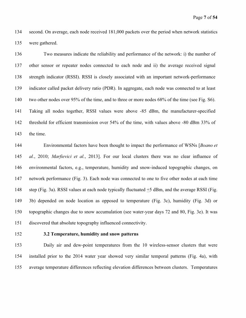
Figure 1. a) Location of American River basin and 14 sensor clusters deployed in the upper part 561
of the basin. b) WSN nodes on hypsometric curve with existing snow pillows 562
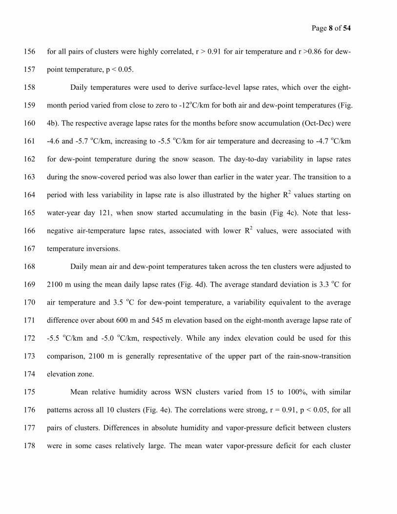
Figure 2. Node layout and steady-state network connections (green lines) at ALP, overlain on 563
Google Map. Sensor nodes are numbered. Two possible paths of data out from sensor node 5 to 564
the base station are marked with red arrows. 565
Figure 3. Network performance of sensor nodes 2,7 and 10 at ALP: a) hourly data of network 566
neighbors number, b) the corresponding average RSSI, c) average air temperature, d) hourly 567
average humidity, and e) daily average snow depth. Shaded periods represent precipitation 568
events. For clarity, data from three sensor nodes are presented. 569
Figure 4. Data from 10 clusters for 8-month period: a) cluster-mean daily averaged air (black 570
traces) and dew-point (red traces) temperature, b) air and dew-point temperature lapse rates, c) 571
R2 value of daily lapse rates, d) mean (dashed lines) and standard deviation (shading) of site air 572
and dew-point temperatures adjusted to 2100 m elevation using the daily lapse rate, e) mean 573
daily average relative humidity, and f) mean daily vapor-pressure deficit calculated from mean 574
daily temperature and relative humidity of each cluster. Shaded periods represent precipitation 575
events. Data for only 10 of the 14 local clusters are shown, as 4 were brought online after the 576
period reported here. 577
Figure 5. Daily mean (µ) and standard deviation (σ) of snow depth from the WSN clusters and 578
SNODAS, including available operational snow-depth-sensor data (blue dashed), and snow 579

Page 29 of 54
courses (green diamond). See Figure S4 for calculation of SNODAS mean and standard 580
deviation. 581
Figure 6. ANOVA results for 20-day period around peak snow accumulation, for between and 582
within-cluster variations in measurements of: a) hourly and daily temperature, b) hourly and 583
daily relative humidity, and c) daily snow depth. See Fig. S7 for data used in the analysis. 584
Page 30 of 54
585
586
Figure 1. a) Location of American River basin and 14 sensor clusters deployed in the upper part 587
of the basin. b) WSN nodes on hypsometric curve with existing snow pillows 588
589
Page 31 of 54
590
Figure 2. Node layout and steady-state network connections (green lines) at ALP, overlain on 591
Google Map. Sensor nodes are numbered. Two possible paths of data out from sensor node 5 to 592
the base station are marked with red arrows. 593
594
Page 32 of 54
595
596
Figure 3. Network performance of sensor nodes 2,7 and 10 at ALP: a) hourly data of network 597
neighbors number, b) the corresponding average RSSI, c) average air temperature, d) hourly 598
average humidity, and e) daily average snow depth. Shaded periods represent precipitation 599
events. For clarity, data from three sensor nodes are presented. 600
601
Page 33 of 54
602
Figure 4. Data from 10 clusters for 8-month period: a) cluster-mean daily averaged air (black 603
traces) and dew-point (red traces) temperature, b) air and dew-point temperature lapse rates, c) 604
R2 value of daily lapse rates, d) mean (dashed lines) and standard deviation (shading) of site air 605
and dew-point temperatures adjusted to 2100 m elevation using the daily lapse rate, e) mean 606
daily average relative humidity, and f) mean daily vapor-pressure deficit calculated from mean 607
daily temperature and relative humidity of each cluster. Shaded periods represent precipitation 608
events. Data for only 10 of the 14 local clusters are shown, as 4 were brought online after the 609
period reported here. 610
611
Page 34 of 54
612 Figure 5. Daily mean (µ) and standard deviation (σ) of snow depth from the WSN clusters and 613
SNODAS, including available operational snow-depth-sensor data (blue dashed), and snow 614
courses (green diamond). See Figure S4 for calculation of SNODAS mean and standard 615
deviation. 616
Page 35 of 54
617
618
Figure 6. ANOVA results for 20-day period around peak snow accumulation, for between and 619
within-cluster variations in measurements of: a) hourly and daily temperature, b) hourly and 620
daily relative humidity, and c) daily snow depth. See Fig. S7 for data used in the analysis. 621
622
Page 36 of 54
Water Resource Research
Supporting Information for
Technical report: the design and evaluation of a basin-scale wireless sensor network for mountain hydrology
Ziran Zhang1, Steven D. Glaser1, Roger C. Bales1,2, Martha Conklin2, Robert Rice2
and Danny G. Marks3
1Department of Civil and Environmental Engineering, University of California, Berkeley,
Berkeley, USA.
2Sierra Nevada Research Institute and School of Engineering, University of California,
Merced, Merced, USA.
3Agricultural Research Service, USDA, Boise, USA.
Page 1 of 54
Introduction 623
This document includes supporting texts and figures and table referenced in the main text. 624
Text S1 625
S1.1 Prior WSN deployments for hydrology in remote areas 626
In 2007, a WSN with a few dozen nodes was deployed to a golf course near Almkerk 627
Netherland to monitor soil moisture. The study claimed to be successful but the description and 628
discussion of the wireless network infrastructure, was very brief [Ritsema et al., 2010]. In 2009, 629
a 12-station, 4-month deployment in a 20-km2 catchment in the Swiss Alps measured the spatial 630
variability of meteorological forcing, including temperature and precipitation. The study was 631
conducted over a short time period with rather sparsely distributed stations [Simoni et al., 2011]. 632
Recently, densely deployed sensor arrays have been scaled to a size comparable to the mountain 633
areas being studied. Ninety-nine sensor loggers, within three 40-180 km2 basins, were deployed 634
to monitor snow properties in southern Germany for one winter. The system deployed used data 635
loggers rather than a WSN [Pohl et al., 2014]. In another study, 150 wireless nodes with over 636
600 soil-moisture sensors were installed in a forest catchment at Westebach, Germany to study 637
the spatiotemporal distribution of soil moisture over complex terrain [Bogena et al., 2010]. The 638
study used a variation of ZigBee motes developed by JenNet Ltd. Over 300 sensors hosted by 60 639
wireless nodes have been deployed at the Southern Sierra Critical Zone Observatory since 2008 640
to study heterogeneous interactions of water within the snowpack, canopy and soil influence on 641
the water cycle [Kerkez et al., 2012]. This installation suffered from network optimization issues 642
that limited locations of the sensor nodes, and hardware problems with the cold. 643
644

Page 2 of 54
S1.2 Present Solutions for Wireless Sensor Networks – A comparison of existing 645
technologies 646
Sensor networks are made up of motes. This term, from its definition “a small speck of 647
dust,” was coined at UC Berkeley to describe a very small, low-power device that incorporates a 648
radio transceiver, computational power, data storage, and sensors. There are many commercially 649
available motes with many different standards. Different motes were designed for different 650
purposes such as research, education, hobbyists, indoor industrial and outdoor monitoring and 651
control applications. The question is why pick one hardware solution over another? Our primary 652
consideration focuses on how well the networking protocols were implemented to ensure 653
performance and robustness. We also look into the hardware flexibility to satisfy needs for 654
interfacing with different sensors. We focus on the most popular of motes that comply with the 655
IEEE 802.11.15.4 standards for power-savings reasons and availability. Properties and 656
specifications of two main families of motes along with our solutions were investigated. 657
S1.2.1 Mica-II, Iris, TelosB, Lotus 658
Memsic Inc. provides a number of low-power motes (MICA, TelosB, and Lotus) that are 659
1802.11.5.4 compatible. The MICA and TelosB design goes back almost twenty years to the 660
early UC Berkeley work. The LOTUS mote with a Cortex M3 processor and ZigBee radio 661
provides the most internal memory for the OS and application software among Memsic motes. 662
Several operating systems (RTOS, MoteRunner and TinyOS) can be ported to LOTUS. However, 663
some problems with the network-routing protocol and channel-management protocols remain. 664
Operating on a single channel makes them vulnerable to network instabilities resulting from 665
signal interference and multi-path effects. The current draw from the LOTUS and MDA300 666
board is estimated to be around 17 mA at 3V when transmitting. The mote depletes two AA 667

Page 3 of 54
batteries in approximately one month when set to transmit for 3 seconds every 3 min. The data-668
acquisition board (MDA300) provides seven single-ended and one (multiplexed to four) 669
differential 12-bit ADC channels; digital I/O support is very limited on this board. 670
S1.2.2 ZigBee and Xbee 671
ZigBee-based motes represent a popular family of wireless motes that share common 672
communication protocols and specifications (network layer and application layer) by 673
implementing a ZigBee software stack [ZigBee, 2009]. In practice ZigBee operates as a star 674
network. Although it is theoretically possible to form a mesh-like network topology, a subset of 675
motes has to be pre-selected and programed as dedicated routing nodes to relay data from the 676
end/leaf node to the coordinator. The RX channel of those router elements has to be constantly 677
powered, which results in high overall energy consumption [Horvat, 2012]. ZigBee operates on a 678
single channel, making it difficult to avoid channel interference due to other ISM sources such as 679
WI-FI, and multipath [Accettura and Piro, 2014]. ZigBee networks are also not able to meet the 680
reliability and latency requirement for industrial applications [Gungor and Hancke, 2009; Huang 681
et al., 2012]. The October 2016 DoS attack on the U.S. web was based on captured zigbee IoT 682
devices, indicating a severe lack of network security. 683
Digi International maintains a family of motes called Xbee. The XBee 2.4 GHz-band 684
mote has its own proprietary protocol called DigiMesh that suffers from environmental 685
interference and varying effects of multipath because it does not implement channel hopping 686
[International, 2009]. In order to achieve low power in a DigiMesh network, the system needs to 687
enter a synchronized sleep mode. Due to the lack of a central network coordinator, a subset of 688
the DigiMesh motes needs to be constantly running to serve as sleep coordinators (i.e., network 689
manager). Those motes continuously broadcast sync message to the surrounding nodes to keep 690

Page 4 of 54
the network assembled, otherwise the message transmitted to a mote during the sleeping period 691
will be permanently lost [International, 2009]. Another possible issue for DigiMesh networks in 692
synchronized sleep mode is that when a new mote is added to the network, it needs to be 693
physically near a sleep coordinator to receive a sync message in order to join the network [Xbee-694
pro and Rf, n.d.]. If a node temporarily drops out, it is permanently lost, and an extended trial 695
and error installation is difficult to carry out. Xbees are commonly interfaced with Arduino 696
single-board computers to provide facilities to host sensors, compute, and store data. The 697
Arduino Uno R3, with no external load from sensors and other components, consumes about 40 698
mA at 5V. The Uno R3 uses a slow and outdated Atmega328P (8-bit/16MHz) microprocessor 699
with a 10-bit analog to digital converter that provides only six analog pins and fourteen digital 700
pins to interface with the sensors and other equipment. Similar issues with power and flexibility 701
can be found with solutions provided by Raspberry Pi, which consumes 700 mA at 5V, making it 702
impractical to operate with a battery. Systems with Arduino and Raspberry Pi are best kept 703
indoors where sufficient power input is provided. They are not recommended for long-term 704
outdoor deployments, as they were designed for hobbyist use. 705
S1.2.3 Metronome Systems neoMote 706
Metronome Systems provides a comprehensive solution for the sensor node called the 707
neoMote, which was developed by UC Berkeley researchers. It combines the DUST Networks 708
Eterna radio module with a Cypress Programmable System on Chip (PSoC5) into a two-chip 709
mote solution. While DUST Network radios provide robust and reliable wireless networking 710
capability, PSoC provides full support to any sensor or control peripheral. The PSoC offers an 711
array of configurable system blocks that can be dynamically added to a project for a particular 712
application. For instance, the board can interface up to 40 analog and/or digital sensors at once, 713

Page 5 of 54
providing all analog and digital signal conditioning and excitation. The PSoC building blocks are 714
available to a drag-and-drop interface and are reprogrammable over the radio. The neoMote 715
provides 3.3, 5, and 12Vdc excitation to sensors. Interfacing with a SD-card slot provides 716
additional storage for data and system parameters. In addition, the board is ultra-low power. 717
Power consumption is 30 µA, 60 µA in 20-bit A/D mode, with transmission adding 10 mA - two 718
to three orders of magnitude lower than the previous solutions. The network is controlled by a 719
Metronome Systems network manager, which also interfaces the data with the outside world. It 720
is based on a full LINUX computer, while only consuming 50 mA at 5V. It runs a full database 721
and sends the data out through a variety of modems. 722
DUST Networks, a division of Linear Technology, provides an industrially rated ultra-723
low power fully meshed wireless networking platform. The dynamic network allows seamless 724
joining and rejoining by any mote or hopper. A few technical details properties of the DUST 725
mote make it superior to other choices. The SmartMesh IP software utilizes time synchronized 726
mesh protocol (TSMP) that maintains complete network synchronization to 10 µs, which 727
minimizes the “on-time” to listen for the beacon. Incorporating Time-Slotted Channel Hopping 728
(TSCH) reduces interference within the communication channels through diversity of frequency 729
at which each packet is sent [Pister and Doherty, 2008]. Adding diversity to the channel 730
selection reduces the adverse effect of multipath fading in wireless network. The typical duty 731
cycle of the DUST radio module is < 1% while keeping communication reliability 99.999%. 732
The DUST network is unique in that it constantly collects a wide variety of network statistics, 733
which allows for the later optimization of a network. 734
Page 6 of 54
The Metronome system provides capability for Internet-of-Things functionalities, such 735
that one can deliver programs remotely to sensor nodes to resync real-time clock settings, change 736
firmware, sampling interval, sensor gain, etc. 737
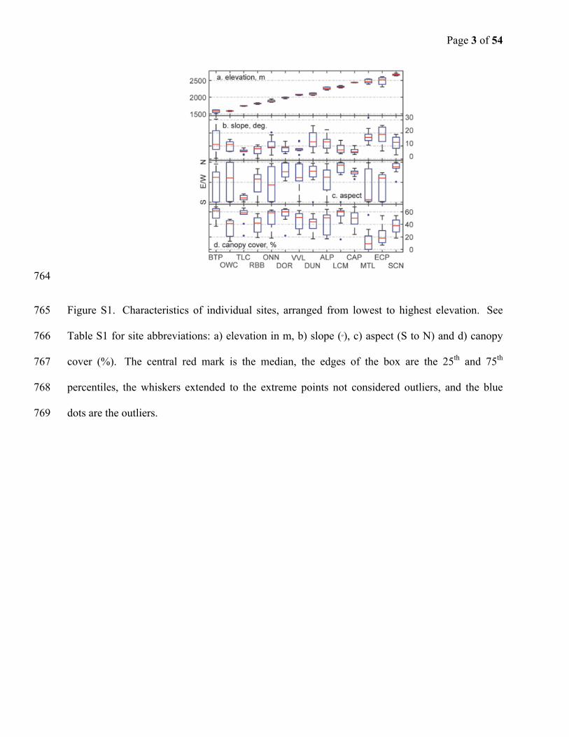
S2 Physiographic attributes of cluster 738
Elevations were extracted from a 30-m DEM. Slopes and aspects were calculated using 739
ArcGIS spatial analyst toolbox. Percent canopy cover was extracted from NLCD 2011 data layer 740
[Jin et al., 2013]. Overall, sensor placement reflects a close correspondence between site 741
characteristic of the sensor nodes and the features within the 1-km2 areas for most of the sites. 742
Mean site elevations range from 1590 to 2680 m, with considerable overlap between some sites 743
(Fig. S1a). Some sites are relatively flat (e.g. CAP) and some on relatively steeper terrain (e.g. 744
MTL, ECP) (Fig. S1b). It was possible to get a range of aspect at most sites, with the notable 745
exception of TLC and CAP (Fig S1c). All other sites have both north and south aspects. Sensor 746
placements capture the range of canopy covers, shown in Fig. S1d. 747
S3 Details of sensor nodes 748
Each sensor node (Fig. S3) is equipped with an ultrasonic snow-depth sensor (Judd 749
Communication Depth Sensor) and a temperature/relative humidity sensor (Sensirion SHT-15). 750
A selected subset of the nodes at five of the sites measure soil moisture and soil temperature 751
(Decagon GS3) at depths of 10 and 60 cm. Nine sites include measurements of total incoming 752
solar radiation using an upward-pointing Hukseflux-LP02 pyranometer on a separate mast with a 753
concrete foundation. The solar-radiation sensors at these locations are located in the open, 754
without obstruction by either canopy or the terrain to capture the total available incoming solar 755
irradiance. At nine of the 14 sites, co-located with the clear-sky irradiance, solar radiation is 756

Page 7 of 54
measured in a partially canopy-covered location, providing representative solar irradiance-757
measurements underneath the canopy structure. The accuracy and the resolution of the sensors is 758
described in Table S2. It should be noted that our wireless nodes are not limited to these sensors, 759
which were chosen based on past performance, cost and consistency with other networks. 760
Page 1 of 54
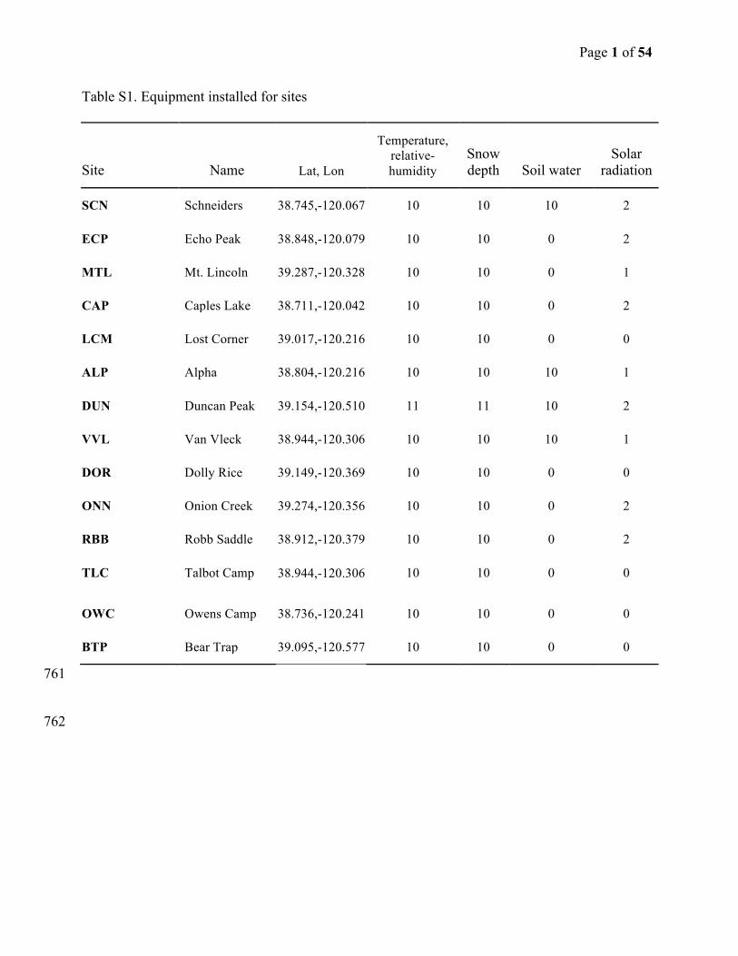
Table S1. Equipment installed for sites
Site
Name Lat, Lon
Temperature, relative-humidity
Snow depth Soil water
Solar radiation
SCN Schneiders 38.745,-120.067 10 10 10 2
ECP Echo Peak 38.848,-120.079 10 10 0 2
MTL Mt. Lincoln 39.287,-120.328 10 10 0 1
CAP Caples Lake 38.711,-120.042 10 10 0 2
LCM Lost Corner 39.017,-120.216 10 10 0 0
ALP Alpha 38.804,-120.216 10 10 10 1
DUN Duncan Peak 39.154,-120.510 11 11 10 2
VVL Van Vleck 38.944,-120.306 10 10 10 1
DOR Dolly Rice 39.149,-120.369 10 10 0 0
ONN Onion Creek 39.274,-120.356 10 10 0 2
RBB Robb Saddle 38.912,-120.379 10 10 0 2
TLC Talbot Camp 38.944,-120.306 10 10 0 0
OWC Owens Camp 38.736,-120.241 10 10 0 0
BTP Bear Trap 39.095,-120.577 10 10 0 0
761
762

Page 2 of 54
TableS2.Sensorsusedforfieldmonitoring
SensirionSHT-15temperature/relativehumiditysensor
2%rHaccuracy
12-bitdigitalresolutionrH
0.3°Ctemperatureaccuracy
14-bittemperatureresolution
factorycalibration
digitalinterface
JuddUltrasonicDepthSensor
0.5to10mrange
0.4%distancetotargetdistanceaccuracy
digitaloranalogoutput
calibratedinthefield
DecagonGS3SoilVolumetricWatercontentandTemperatureSensor
±0.03m3/m3(±3%VWC)volumetricwatercontentaccuracy
complexresistivity-typemeasurementtechnique
±1°Csoiltemperatureaccuracy
3.6VTTLoutput
HuksefluxLP02Pyranometer
secondclassspecifications
285to3000x10-9mspectralrange
15x10-6V/(W/m2)sensitivity
763
Page 3 of 54
764
Figure S1. Characteristics of individual sites, arranged from lowest to highest elevation. See 765
Table S1 for site abbreviations: a) elevation in m, b) slope (o), c) aspect (S to N) and d) canopy 766
cover (%). The central red mark is the median, the edges of the box are the 25th and 75th 767
percentiles, the whiskers extended to the extreme points not considered outliers, and the blue 768
dots are the outliers. 769
Page 4 of 54
770
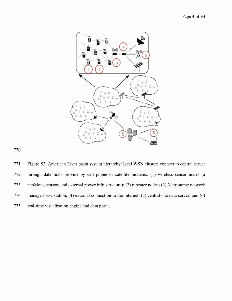
Figure S2. American River basin system hierarchy: local WSN clusters connect to central server 771
through data links provide by cell phone or satellite modems: (1) wireless sensor nodes (a 772
neoMote, sensors and external power infrastructure); (2) repeater nodes; (3) Metronome network 773
manager/base station; (4) external connection to the Internet; (5) central-site data server; and (6) 774
real-time visualization engine and data portal. 775
Page 5 of 54
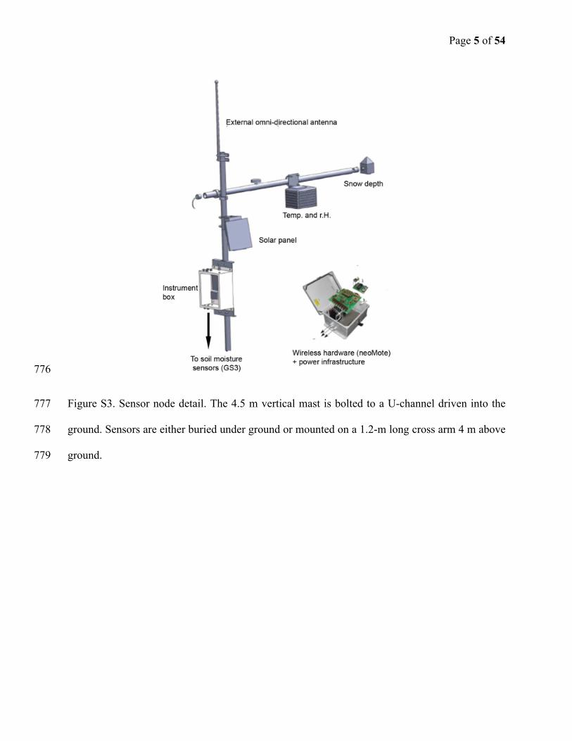
776
Figure S3. Sensor node detail. The 4.5 m vertical mast is bolted to a U-channel driven into the 777
ground. Sensors are either buried under ground or mounted on a 1.2-m long cross arm 4 m above 778
ground. 779
Page 6 of 54
780
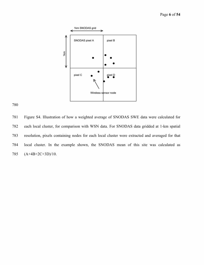
Figure S4. Illustration of how a weighted average of SNODAS SWE data were calculated for 781
each local cluster, for comparison with WSN data. For SNODAS data gridded at 1-km spatial 782
resolution, pixels containing nodes for each local cluster were extracted and averaged for that 783
local cluster. In the example shown, the SNODAS mean of this site was calculated as 784
(A+4B+2C+3D)/10. 785
Page 7 of 54
786
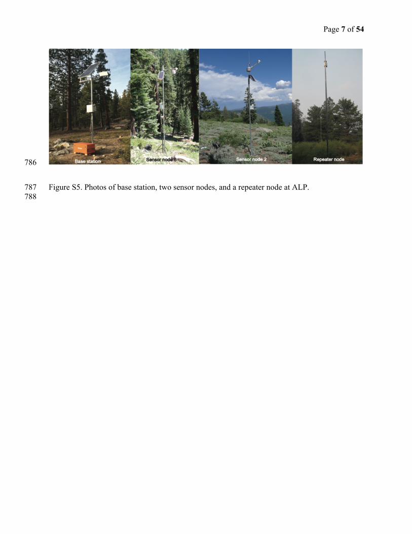
Figure S5. Photos of base station, two sensor nodes, and a repeater node at ALP. 787 788
Page 8 of 54
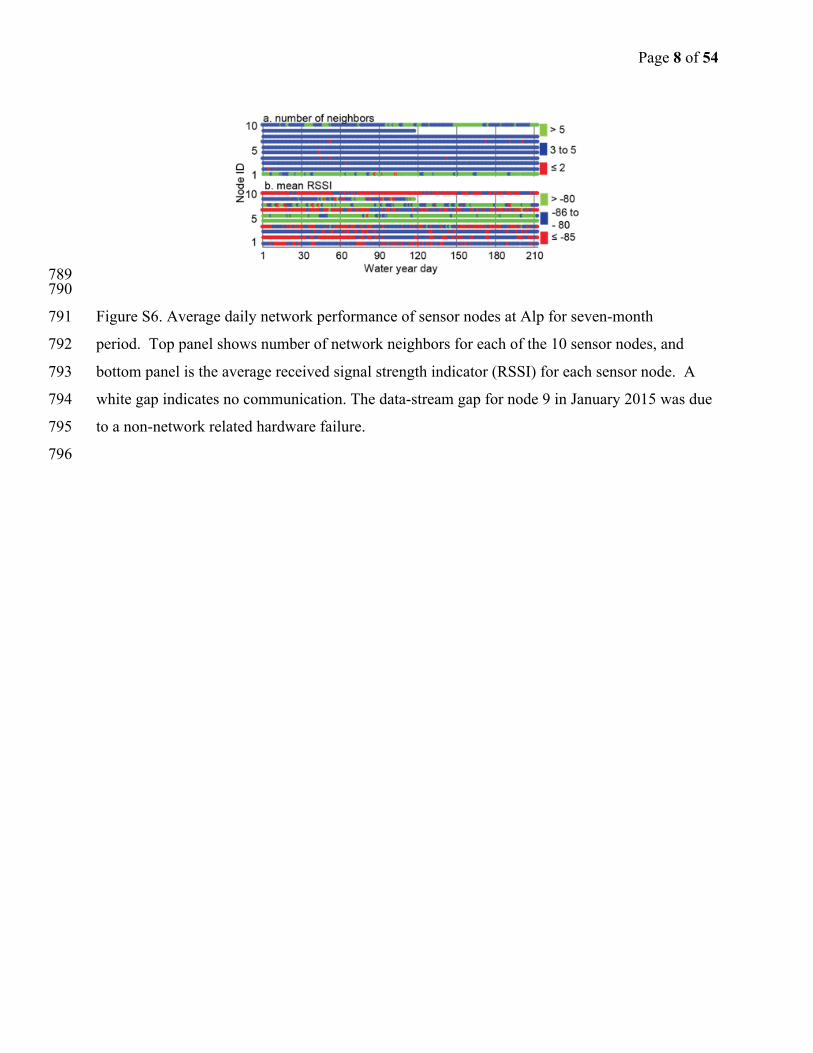
789 790
Figure S6. Average daily network performance of sensor nodes at Alp for seven-month 791
period. Top panel shows number of network neighbors for each of the 10 sensor nodes, and 792
bottom panel is the average received signal strength indicator (RSSI) for each sensor node. A 793
white gap indicates no communication. The data-stream gap for node 9 in January 2015 was due 794
to a non-network related hardware failure. 795
796
Page 9 of 54
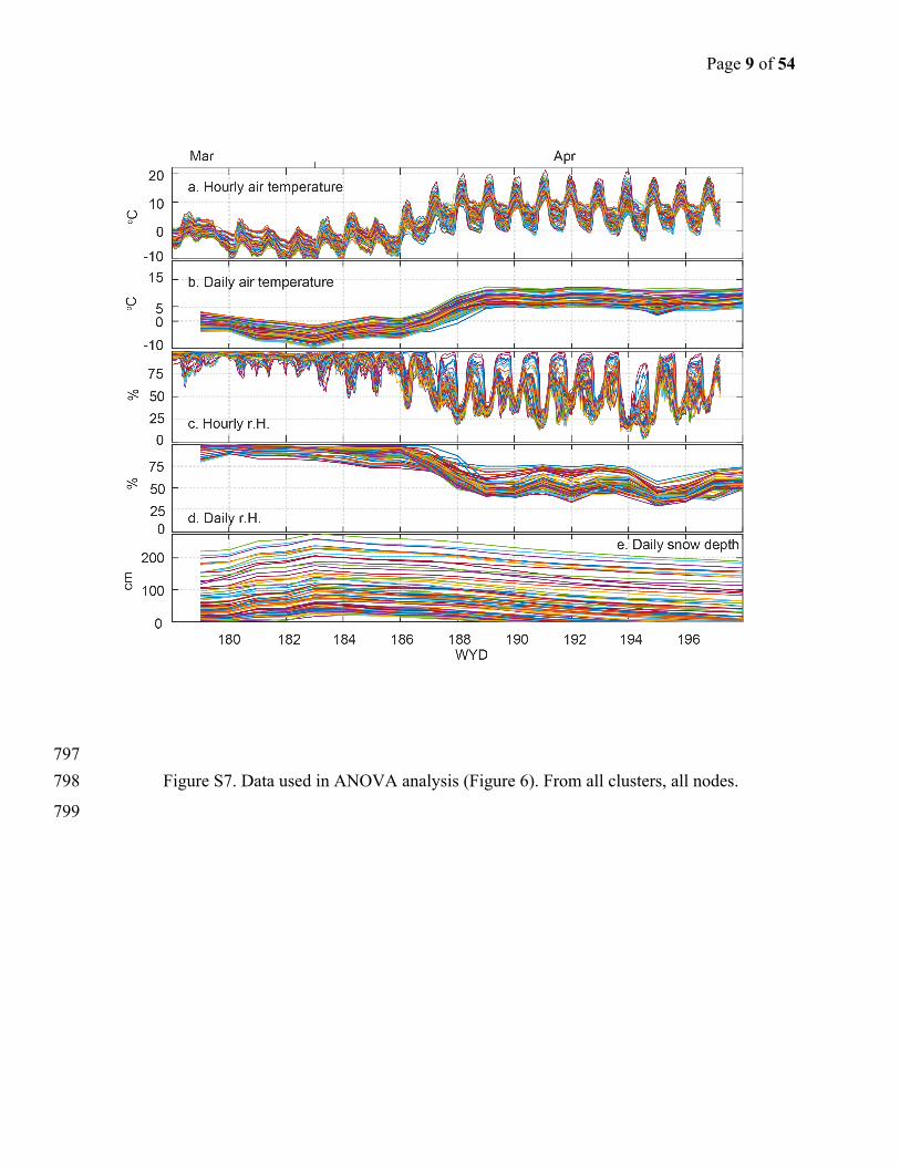
797 Figure S7. Data used in ANOVA analysis (Figure 6). From all clusters, all nodes. 798
799
Page 10 of 54
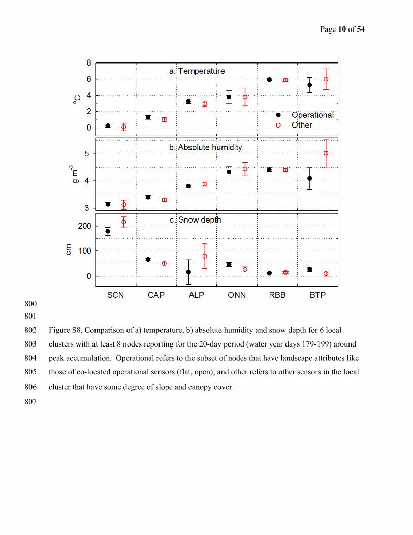
800 801
Figure S8. Comparison of a) temperature, b) absolute humidity and snow depth for 6 local 802
clusters with at least 8 nodes reporting for the 20-day period (water year days 179-199) around 803
peak accumulation. Operational refers to the subset of nodes that have landscape attributes like 804
those of co-located operational sensors (flat, open); and other refers to other sensors in the local 805
cluster that have some degree of slope and canopy cover. 806
807