Finite-size analysis of unidimensional continuous-variable ... Express.25(23... · Finite-size analysis of unidimensional continuous -variable quantum key ... J. Cerf, and P . Grangier

Finite-size analysis of unidimensional continuous-variable quantum key distribution under realistic conditions PU WANG,1 XUYANG WANG,1,2,4 JUNQI LI,3 AND YONGMIN LI1,2,* 1State Key Laboratory of Quantum Optics and Quantum Optics Devices, Institute of Opto-Electronics, Shanxi University, Taiyuan 030006, China 2Collaborative Innovation Center of Extreme Optics, Shanxi University, Taiyuan 030006, China 3Institute of Theoretical Physics, Shanxi University, Taiyuan 030006, China [email protected] *[email protected]

Abstract: We analyze the unidimensional (UD) continuous-variable quantum key distribution protocol in a finite size scenario under realistic conditions. The dependence of the secret key rate on realistic parameters is analyzed numerically. A method of calculating the optimal ratio to divide the data samples in order to achieve the largest secret key rate is proposed. When the data samples are large, the superiority of the UD protocol in data processing becomes apparent. It is expected that the features and methods presented in this paper will aid in the exploration of the latent capacity of the UD protocol as well as the development of further applications. © 2017 Optical Society of America OCIS codes: (270.5568) Quantum cryptography; (060.5565) Quantum communications.

References and links 1. V. Scarani, H. Bechmann-Pasquinucci, N. J. Cerf, M. Dušek, N. Lütkenhaus, and M. Peev, “The security of

practical quantum key distribution,” Rev. Mod. Phys. 81(3), 1301–1350 (2009).2. C. Weedbrook, S. Pirandola, R. García-Patrón, N. J. Cerf, T. C. Ralph, J. H. Shapiro, and S. Lloyd, “Gaussian

quantum information,” Rev. Mod. Phys. 84(2), 621–669 (2012).3. T. C. Ralph, “Continuous variable quantum cryptography,” Phys. Rev. A 61(1), 010303 (1999). 4. N. J. Cerf, M. Levy, and G. Van Assche, “Quantum distribution of Gaussian keys using squeezed states,” Phys.

Rev. A 63(5), 052311 (2001).5. Ch. Silberhorn, T. C. Ralph, N. Lütkenhaus, and G. Leuchs, “Continuous variable quantum cryptography:

beating the 3 dB loss limit,” Phys. Rev. Lett. 89(16), 167901 (2002).6. F. Grosshans and P. Grangier, “Continuous variable quantum cryptography using coherent states,” Phys. Rev.

Lett. 88(5), 057902 (2002).7. F. Grosshans, G. Van Assche, J. Wenger, R. Brouri, N. J. Cerf, and P. Grangier, “Quantum key distribution

using Gaussian-modulated coherent states,” Nature 421(6920), 238–241 (2003).8. C. Weedbrook, A. M. Lance, W. P. Bowen, T. Symul, T. C. Ralph, and P. K. Lam, “Quantum cryptography

without switching,” Phys. Rev. Lett. 93(17), 170504 (2004).9. A. M. Lance, T. Symul, V. Sharma, C. Weedbrook, T. C. Ralph, and P. K. Lam, “No-switching quantum key

distribution using broadband modulated coherent light,” Phys. Rev. Lett. 95(18), 180503 (2005).10. C. Weedbrook, A. M. Lance, W. P. Bowen, T. Symul, T. C. Ralph, and P. K. Lam, “Coherent-state quantum key

distribution without random basis switching,” Phys. Rev. A 73(2), 022316 (2006).11. R. García-Patrón and N. J. Cerf, “Unconditional optimality of Gaussian attacks against continuous-variable

quantum key distribution,” Phys. Rev. Lett. 97(19), 190503 (2006).12. M. Navascués, F. Grosshans, and A. Acín, “Optimality of Gaussian attacks in continuous-variable quantum

cryptography,” Phys. Rev. Lett. 97(19), 190502 (2006).13. J. Lodewyck, M. Bloch, R. García-Patrón, S. Fossier, E. Karpov, E. Diamanti, T. Debuisschert, N. J. Cerf, R.

Tualle-Brouri, S. W. McLaughlin, and P. Grangier, “Quantum key distribution over 25 km with an all-fiber continuous-variable system,” Phys. Rev. A 76(4), 042305 (2007).

14. R. Renner and J. I. Cirac, “de Finetti representation theorem for infinite-dimensional quantum systems andapplications to quantum cryptography,” Phys. Rev. Lett. 102(11), 110504 (2009).

15. R. García-Patrón and N. J. Cerf, “Continuous-variable quantum key distribution protocols over noisy channels,” Phys. Rev. Lett. 102(13), 130501 (2009).

16. A. Leverrier and P. Grangier, “Unconditional security proof of long-distance continuous-variable quantum key distribution with discrete modulation,” Phys. Rev. Lett. 102(18), 180504 (2009).

Journal © 2017 Received 10 Jul 2017; revised 24 Oct 2017; accepted 25 Oct 2017; published 30 Oct 2017 #302081 https://doi.org/10.1364/OE.25.027995

Vol. 25, No. 23 | 13 Nov 2017 | OPTICS EXPRESS 27995

https://crossmark.crossref.org/dialog/?doi=10.1364/OE.25.027995&domain=pdf&date_stamp=2017-10-30

17. Q. Dinh Xuan, Z. Zhang, and P. L. Voss, “A 24 km fiber-based discretely signaled continuous variable quantum key distribution system,” Opt. Express 17(26), 24244–24249 (2009).

18. L. S. Madsen, V. C. Usenko, M. Lassen, R. Filip, and U. L. Andersen, “Continuous variable quantum key distribution with modulated entangled states,” Nat. Commun. 3, 1083 (2012).

19. F. Furrer, T. Franz, M. Berta, A. Leverrier, V. B. Scholz, M. Tomamichel, and R. F. Werner, “Continuousvariable quantum key distribution: finite-key analysis of composable security against coherent attacks,” Phys. Rev. Lett. 109(10), 100502 (2012).

20. P. Jouguet, S. Kunz-Jacques, A. Leverrier, P. Grangier, and E. Diamanti, “Experimental demonstration of long-distance continuous-variable quantum key distribution,” Nat. Photonics 7, 378–381 (2013).

21. X. Y. Wang, Z. L. Bai, S. F. Wang, Y. M. Li, and K. C. Peng, “Four-state modulation continuous variable quantum key distribution over a 30-km fiber and analysis of excess noise,” Chin. Phys. Lett. 30(1), 010305(2013).

22. T. Gehring, V. Händchen, J. Duhme, F. Furrer, T. Franz, C. Pacher, R. F. Werner, and R. Schnabel, “Implementation of continuous-variable quantum key distribution with composable and one-sided-device-independent security against coherent attacks,” Nat. Commun. 6, 8795 (2015).

23. B. Qi, P. Lougovski, R. Pooser, W. Grice, and M. Bobrek, “Generating the local oscillator “Locally” incontinuous-variable quantum key distribution based on coherent detection,” Phys. Rev. X 5(4), 041009 (2015).

24. D. Huang, P. Huang, D. Lin, and G. Zeng, “Long-distance continuous-variable quantum key distribution by controlling excess noise,” Sci. Rep. 6, 19201 (2016).

25. Y. M. Li, X. Y. Wang, Z. L. Bai, W. Y. Liu, S. S. Yang, and K. C. Peng, “Continuous variable quantum key distribution,” Chin. Phys. B 26, 040303 (2017).

26. S. Pirandola, C. Ottaviani, G. Spedalieri, C. Weedbrook, S. L. Braunstein, S. Lloyd, T. Gehring, C. S. Jacobsen, and U. L. Andersen, “High-rate measurement-device-independent quantum cryptography,” Nat. Photonics 9, 397–402 (2015).

27. P. Papanastasiou, C. Ottaviani, and S. Pirandola, “Finite size analysis of measurement device independent quantum cryptography with continuous variables,” https://arxiv.org/abs/1707.04599.

28. C. Lupo, C. Ottaviani, P. Papanastasiou, and S. Pirandola, “CV MDI QKD: Composable Security against Coherent Attacks,” https://arxiv.org/abs/1704.07924.

29. S. Fossier, E. Diamanti, T. Debuisschert, A. Villing, R. Tualle-Brouri, and P. Grangier, “Field test of a continuous-variable quantum key distribution prototype,” New J. Phys. 11(4), 045023 (2009).

30. P. Jouguet, S. Kunz-Jacques, T. Debuisschert, S. Fossier, E. Diamanti, R. Alléaume, R. Tualle-Brouri, P. Grangier, A. Leverrier, P. Pache, and P. Painchault, “Field test of classical symmetric encryption withcontinuous variables quantum key distribution,” Opt. Express 20(13), 14030–14041 (2012).

31. D. Huang, P. Huang, H. Li, T. Wang, Y. Zhou, and G. Zeng, “Field demonstration of a continuous-variable quantum key distribution network,” Opt. Lett. 41(15), 3511–3514 (2016).

32. V. C. Usenko and F. Grosshans, “Unidimensional continuous-variable quantum key distribution,” Phys. Rev. A92(6), 062337 (2015).

33. T. Gehring, C. S. Jacobsen, and U. L. Andersen, “Single-quadrature continuous-variable quantum keydistribution,” Quantum Inf. Comput. 16(13), 1081–1095 (2016).

34. X. Y. Wang, W. Y. Liu, P. Wang, and Y. M. Li, “Experimental study on all-fiber-based unidimensionalcontinuous-variable quantum key distribution,” Phys. Rev. A 95(6), 062330 (2017).

35. A. Leverrier, F. Grosshans, and P. Grangier, “Finite-size analysis of a continuous-variable quantum key distribution,” Phys. Rev. A 81(6), 062343 (2010).

36. X. Y. Wang, Z. L. Bai, P. Y. Du, Y. M. Li, and K. C. Peng, “Ultrastable fiber-based time-domain balancedhomodyne detector for quantum communication,” Chin. Phys. Lett. 29(12), 124202 (2012).

37. B. Qi, L. L. Huang, L. Qian, and H. K. Lo, “Experimental study on the Gaussian-modulated coherent-state quantum key distribution over standard telecommunication fibers,” Phys. Rev. A 76(5), 052323 (2007).

38. L. Ruppert, V. C. Usenko, and R. Filip, “Long-distance continuous-variable quantum key distribution withefficient channel estimation,” Phys. Rev. A 90(6), 062310 (2014).

39. O. Thearle, S. M. Assad, and T. Symul, “Estimation of output-channel noise for continuous-variable quantum key distribution,” Phys. Rev. A 93(4), 042343 (2016).

40. Z. Qu and I. B. Djordjevic, “High-speed free-space optical continuous-variable quantum key distribution enabledby three-dimensional multiplexing,” Opt. Express 25(7), 7919–7928 (2017).

41. A. Leverrier, “Composable security proof for continuous-variable quantum key distribution with coherent States,” Phys. Rev. Lett. 114(7), 070501 (2015).

42. A. Leverrier, “Security of Continuous-Variable Quantum Key Distribution via a Gaussian de Finetti Reduction,” Phys. Rev. Lett. 118(20), 200501 (2017).

1. IntroductionQuantum key distribution (QKD) allows two remote and legal parties, Alice and Bob, to share a common secret key in a quantum channel, which is assumed to be controlled by a potential eavesdropper Eve, and an authenticated classical channel [1,2]. As a safe and advanced communication method, its security is based on the basic principles of quantum mechanics.


#302081 https://doi.org/10.1364/OE.25.027995


Unlike discrete-variable QKD, continuous-variable (CV) QKD encodes the information into continuous-spectrum quantum observables and utilizes homodyne detectors instead of single-photon detectors. During the past decade, the theory and technology of CV QKD have undergone rapid development [3–28]. It is known that CV QKD protocols based on non-classical states demonstrate better performance than those based on coherent states. However, as the coherent state is easier to generate and only requires classical telecom technologies, coherent state based protocols have developed rapidly. Prototype machines have been developed, and several field tests have been completed [29–31]. It is believed that protocols based on coherent states can be used in practical applications in near future.

A further simplified unidimensional (UD) CV QKD protocol based on coherent states has recently been proposed [32]. Nearly simultaneously to this development, UD CV QKD was realized experimentally [33,34]. This asymmetric UD coherent state protocol allows the sender, Alice, to use one modulator instead of two, thereby reducing the complexity and cost of Alice’s apparatus. However, all previous works failed to take into account the finite-size effects, which are critical to the practical security of the QKD system.

In this paper, we mainly analyze the UD CV QKD protocol in a finite size scenario under realistic conditions. Firstly, in order to lay a good foundation, an introduction to the UD protocol under realistic conditions is presented. The analytic expression for the symplectic eigenvalues, which are used to calculate the secret key rate, is derived in order to significantly reduce the calculation time. Next, the dependence of the asymptotic secret key rate on realistic parameters, which will provide a useful guide for parameter selection, is investigated. When the amount of data samples used for parameter estimation is large in the finite size scenario, the secret key rate will approach the asymptotic secret key rate.

Unlike with the symmetrical (SY) coherent state protocol [7, 13], in the UD protocol we must estimate the transmission efficiency and excess noise of one quadrature, as well as the variance of the other quadrature. It is well known that the larger the amount of data samples used for parameter estimation, the weaker the finite size effect [35]. However, taking into consideration the real-time and stability of the QKD system, taking a longer period of time to increase the total number of samples is not necessarily beneficial. In order to distill the largest secret key rate from a limited total number of samples, a method is proposed to subdivide the data samples with an optimal ratio. After comparison, we can see that the UD protocol can achieve similar performance to its SY counterpart under realistic conditions, when the excess noise is low and number of samples is large. In particular, when the amount of data samples is large, the superiority of the UD protocol in data processing emerges.

In Sec. II, the UD CV QKD protocol under realistic conditions is presented, and the security under collective attack is analyzed using the entanglement-based (EB) scheme. Section III provides the numerical analysis of the secret key rate, depending on realistic parameters such as the reconciliation efficiency, detection efficiency, and electronic noise. Section IV presents the method of calculating the optimal ratio to divide the data samples in order to achieve the largest secret key rate under Gaussian collective attack in a finite size scenario. Finally, Section V presents the conclusions.

2. Unidimensional protocol under realistic conditions2.1 An introduction to unidimensional protocol schemes

The prepare-and-measure (PM) scheme is shown in Fig. 1(a). The sender, Alice, displaces independent coherent states produced by a laser to a Gaussian distribution in the amplitude or phase quadrature, using one amplitude or phase modulator with a modulation variance MV . Note that the variances in this paper are all normalized to shot noise units. The Gaussian-modulated quantum states form a unidimensional chain structure in phase space with a length of 1MV + and a thickness of 1. Alice sends these quantum states to Bob through an


#302081 https://doi.org/10.1364/OE.25.027995


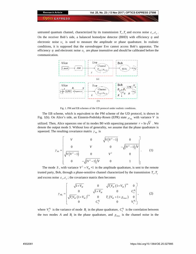
untrusted quantum channel, characterized by its transmission ,x yT T and excess noise ,x yε ε . On the receiver Bob’s side, a balanced homodyne detector (BHD) with efficiency η and electronic noise eυ is used to measure the amplitude or phase quadrature. In realistic conditions, it is supposed that the eavesdropper Eve cannot access Bob’s apparatus. The efficiency η and electronic noise eυ are phase insensitive and should be calibrated before the communication.

Fig. 1. PM and EB schemes of the UD protocol under realistic conditions.

The EB scheme, which is equivalent to the PM scheme of the UD protocol, is shown in Fig. 1(b). On Alice’s side, an Einstein-Podolsky-Rosen (EPR) state

0ABρ with variance V is

utilized. Then, Alice squeezes one of its modes B0 with squeezing parameter lnr V= . We denote the output mode S. Without loss of generality, we assume that the phase quadrature is squeezed. The resulting covariance matrix ASγ is

( )( )

( )( )

2

2

2 2

2

0 1 0

0 0 1.

1 0 0

0 1 0 1

AS

V V V

V V V

V V V

V V

γ

−

− − = − − −

(1)

The mode S , with variance 2 +1MV V= in the amplitude quadrature, is sent to the remote trusted party, Bob, through a phase-sensitive channel characterized by the transmission ,x yT Tand excess noise ,x yε ε ; the covariance matrix then becomes

( )

( ) ( )

1

1

1 1

1 4

y1 4

y

1 0 1 0

0 1 0,

1 0 1 00 0

M x M M

BM

AB

x M M x M linexB B

y

V T V V

V C

T V V T VC V

γχ

+ + +

= + + +

(2)

where 1ByV is the variance of mode 1B in the phase quadrature, 1

yBC is the correlation between

the two modes A and 1B in the phase quadrature, and linexχ is the channel noise in the


#302081 https://doi.org/10.1364/OE.25.027995


amplitude quadrature and can be expressed as ( )1linex x x xT Tχ ε= − + . Because there is no

modulation in the phase quadrature, the correlation 1yBC cannot be estimated.

In the EB scheme, the realistic BHD can be modeled as a beam splitter with transmission η and a perfect BHD. The electronic noise eV of the realistic BHD can be modeled as a thermal state

0Rρ , which could be considered to be the reduced state obtained from an EPR

state 0R Hρ with variance NV entering the other input port of the beam splitter. The variance

NV has a relationship with eυ given by ( )1e1 -NV υ η= + . After the beam splitter, the covariance matrix ABγ has the form

( )

( ) ( )

1 4

1 4

1 0 1 0

0 1 0,

1 0 1 00 0

M x M M

BM y

AB

x M M x M totxB By y

V T V V

V C

T V V T VC V

η

γη η χ

+ + +

= + + +

(3)

where hom /totx linex xTχ χ χ= + is the total noise added between Alice and Bob relative to the channel input in the amplitude quadrature, and ( )hom 1 /eVχ η η η= − + is the total noise

introduced by the realistic BHD relative to Bob’s input in the amplitude quadrature. ByV is the

variance of mode B in the phase quadrature. The noise homχ , which is phase insensitive, has the same value in both the amplitude and phase quadrature. y

BC is the correlation between the

two modes A and B in the phase quadrature. ByV and B

yC are related to 1ByV and 1B

yC as follows

( )1 1hom . B BB B

y y y yV V and C Cη χ η= + = (4)

2.2 Security analysis

In the asymptotic limit, the collective attack has been proven to be the optimal attack [14] and the corresponding secret key rate is given by

,AB BEK Iβ χ∞ = ⋅ − (5)

where ABI is the Shannon mutual information between Alice and Bob, BEχ represents the Holevo bound between Bob and Eve for reverse reconciliation, and β is the reverse reconciliation efficiency. The mutual information can be calculated by the following expression

21 log 1 .2 1

MAB

totx

VIχ

= + +

(6)

The Holevo bound is defined as

( )( ) S ,BxBE E ESχ ρ ρ= − (7)

where ( )ES ρ is the von Neumann entropy of the eavesdropper’s quantum state Eρ , and ( )Bx

ES ρ is the conditional von Neumann entropy. As 1

( ) ( )AB ES Sρ ρ= and ( ) ( )B Bx xE ARHS Sρ ρ=

[13], we can rewrite BEχ as


#302081 https://doi.org/10.1364/OE.25.027995


1( ) ( ).Bx

BE AB ARHS Sχ ρ ρ= − (8) After an elaborate derivation, the analytical expression for the symplectic eigenvalues of

the covariance matrix 1ABγ is

( )2 21,2

1 4 ,2

A A Bλ = ± − (9)

where

( ) ( )11 1141 2 1 ,B

M x M x y M M xB B

y yV V T CV V TA V Vε+ + + + + += (10)

( ) ( )( )( )112

1 1 1 .BBy M y M x xV C V TB V ε+ − + += (11)

The analytical expressions for the symplectic eigenvalues 3,4,5λ of the covariance matrix Bx

ARHγ are

2 23,4 5

1 4 1,2

C C Dλ λ = ± − = (12)

where

(1 ) (( 1)( 2) ),

1e x x M M x

x x M x e

A T V V TC

AT V T

υ ε ηε η η υ

+ + + + + −+ + +

= (13)

(1 ) (1 )(1 )1

e M x x

x x M x e

DB V T

T V Tυ η ε η

ε η η υ+ − + + +

+ + += . (14)

The Holevo bound can be obtained by

( ) ( )1 2 3 4+ - ( ,- ( ) )BE G G G Gχ λ λ λ λ= (15)

where ( ) ( ) ( )2 21 log 1 logG x x x x x= + + − . The variables 1ByC and 1B

yV have uncertainty constrained by the Heisenberg uncertainty principle as

10 ,AB iγ + ⋅Ω ≥ (16)

where =2

1

0 1

1 0

n

k= −

Ω = ⊕ .

We then obtain the parabolic equation

1 12 linex0 0

linex

( ) ( )11

,( )

B BMy y

M

VC C V VV

χχ

− ≤ −++

(17)

where ( )0

11x linex

VT χ

=+

and 00 1 4(1 )

x M

M

V T VC

V= −

+ .

The parabolic curve between 1ByC and 1B

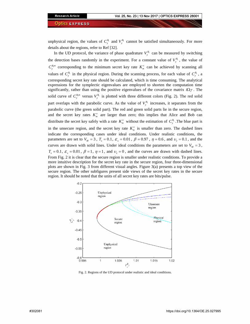
yV is shown in black in Fig. 2. The whole plane is divided into two regions by the parabolic curve, i.e., physical region and unphysical region. The region contained by the parabolic curve is the physical region, which is divided into secure and unsecure regions by the solid cyan curve. In the secure region, the secret key rate is greater than zero. In the unsecure region, the secret key rate is less than zero. In the


#302081 https://doi.org/10.1364/OE.25.027995


unphysical region, the values of 1ByC and 1B

yV cannot be satisfied simultaneously. For more details about the regions, refer to Ref [32].

In the UD protocol, the variance of phase quadrature 1ByV can be measured by switching

the detection bases randomly in the experiment. For a constant value of 1ByV , the value of

1B myC corresponding to the minimum secret key rate mK ∞ can be achieved by scanning all

values of 1ByC in the physical region. During the scanning process, for each value of 1B

yC , a corresponding secret key rate should be calculated, which is time consuming. The analytical expressions for the symplectic eigenvalues are employed to shorten the computation time significantly, rather than using the positive eigenvalues of the covariance matrix i γΩ . The solid curve of 1B m

yC versus 1ByV is plotted with three different colors (Fig. 2). The red solid

part overlaps with the parabolic curve. As the value of 1ByV increases, it separates from the

parabolic curve (the green solid part). The red and green solid parts lie in the secure region, and the secret key rates mK ∞ are larger than zero; this implies that Alice and Bob can distribute the secret key safely with a rate mK ∞ without the estimation of 1B

yC .The blue part is

in the unsecure region, and the secret key rate mK ∞ is smaller than zero. The dashed lines indicate the corresponding cases under ideal conditions. Under realistic conditions, the parameters are set to 3MV = , 0.1xT = , 0.01xε = , 0.97β = , 0.6η = , and 0.1eυ = , and the curves are drawn with solid lines. Under ideal conditions the parameters are set to 3MV = ,

0.1xT = , 0.01xε = , 1β = , 1η = , and 0eυ = , and the curves are drawn with dashed lines. From Fig. 2 it is clear that the secure region is smaller under realistic conditions. To provide a more intuitive description for the secret key rate in the secure region, four three-dimensional plots are shown in Fig. 3 from different visual angles. Figure 3(a) presents a top view of the secure region. The other subfigures present side views of the secret key rates in the secure region. It should be noted that the units of all secret key rates are bits/pulse.

Fig. 2. Regions of the UD protocol under realistic and ideal conditions.


#302081 https://doi.org/10.1364/OE.25.027995


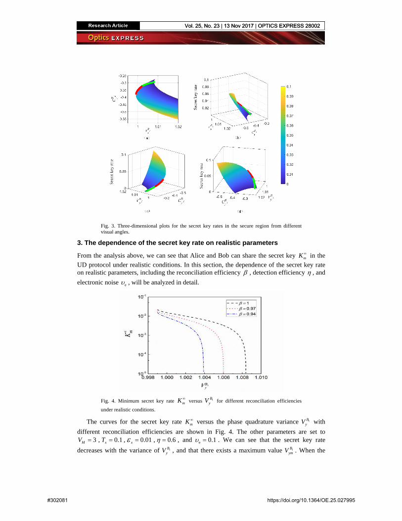
Fig. 3. Three-dimensional plots for the secret key rates in the secure region from different visual angles.

3. The dependence of the secret key rate on realistic parameters

From the analysis above, we can see that Alice and Bob can share the secret key mK ∞ in the UD protocol under realistic conditions. In this section, the dependence of the secret key rate on realistic parameters, including the reconciliation efficiency β , detection efficiency η , and electronic noise eυ , will be analyzed in detail.

Fig. 4. Minimum secret key rate mK ∞ versus 1ByV for different reconciliation efficiencies

under realistic conditions.

The curves for the secret key rate mK ∞ versus the phase quadrature variance 1ByV with

different reconciliation efficiencies are shown in Fig. 4. The other parameters are set to 3MV = , 0.1xT = , 0.01xε = , 0.6η = , and e 0.1υ = . We can see that the secret key rate

decreases with the variance of 1ByV , and that there exists a maximum value 1B

ymV . When the


#302081 https://doi.org/10.1364/OE.25.027995


reconciliation efficiency is higher, the tolerable maximum variance 1BymV in the phase

quadrature is larger. Obviously, a higher secret key rate mK ∞ can be achieved with a higher reconciliation efficiency.

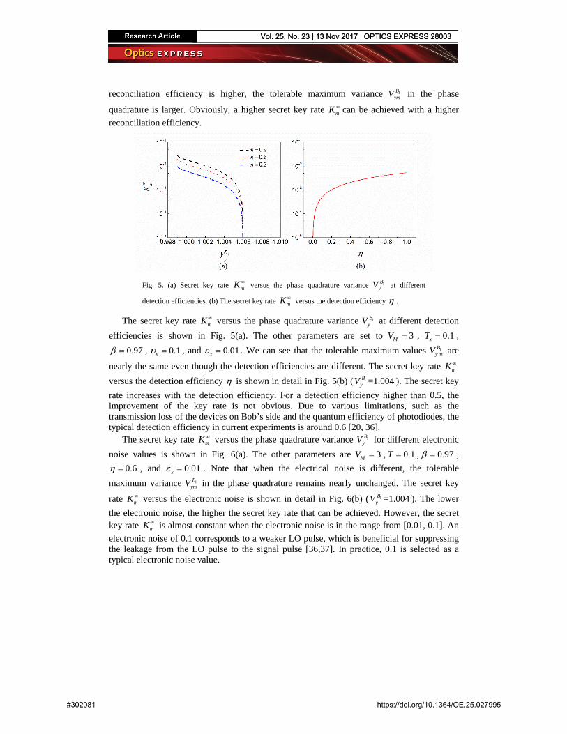
Fig. 5. (a) Secret key rate mK ∞ versus the phase quadrature variance 1ByV at different

detection efficiencies. (b) The secret key rate mK ∞ versus the detection efficiency η .

The secret key rate mK ∞ versus the phase quadrature variance 1ByV at different detection

efficiencies is shown in Fig. 5(a). The other parameters are set to 3MV = , 0.1xT = , 0.97β = , e 0.1υ = , and 0.01xε = . We can see that the tolerable maximum values 1

mB

yV are

nearly the same even though the detection efficiencies are different. The secret key rate mK ∞

versus the detection efficiency η is shown in detail in Fig. 5(b) ( 1 =1.004ByV ). The secret key

rate increases with the detection efficiency. For a detection efficiency higher than 0.5, the improvement of the key rate is not obvious. Due to various limitations, such as the transmission loss of the devices on Bob’s side and the quantum efficiency of photodiodes, the typical detection efficiency in current experiments is around 0.6 [20, 36].

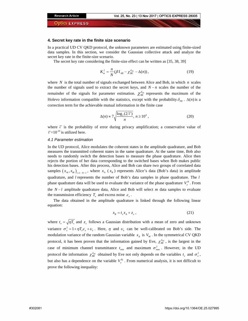
The secret key rate mK ∞ versus the phase quadrature variance 1ByV for different electronic

noise values is shown in Fig. 6(a). The other parameters are 3MV = , 0.1T = , 0.97β = , 0.6η = , and 0.01xε = . Note that when the electrical noise is different, the tolerable

maximum variance 1BymV in the phase quadrature remains nearly unchanged. The secret key

rate mK ∞ versus the electronic noise is shown in detail in Fig. 6(b) ( 1 =1.004ByV ). The lower

the electronic noise, the higher the secret key rate that can be achieved. However, the secret key rate mK ∞ is almost constant when the electronic noise is in the range from [0.01, 0.1]. An electronic noise of 0.1 corresponds to a weaker LO pulse, which is beneficial for suppressing the leakage from the LO pulse to the signal pulse [36,37]. In practice, 0.1 is selected as a typical electronic noise value.


#302081 https://doi.org/10.1364/OE.25.027995


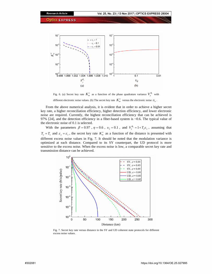
Fig. 6. (a) Secret key rate mK ∞ as a function of the phase quadrature variance 1ByV with

different electronic noise values. (b) The secret key rate mK ∞ versus the electronic noise eυ .

From the above numerical analysis, it is evident that in order to achieve a higher secret key rate, a higher reconciliation efficiency, higher detection efficiency, and lower electronic noise are required. Currently, the highest reconciliation efficiency that can be achieved is 97% [24], and the detection efficiency in a fiber-based system is ~0.6. The typical value of the electronic noise of 0.1 is selected.

With the parameters 0.97β = , 0.6η = , e 0.1υ = , and 1 1By x xV T ε= + , assuming that

y xT T= and y xε ε= , the secret key rate mK ∞ as a function of the distance is presented with different excess noise values in Fig. 7. It should be noted that the modulation variance is optimized at each distance. Compared to its SY counterpart, the UD protocol is more sensitive to the excess noise. When the excess noise is low, a comparable secret key rate and transmission distance can be achieved.

Fig. 7. Secret key rate versus distance in the SY and UD coherent state protocols for different excess noise values.


#302081 https://doi.org/10.1364/OE.25.027995


4. Secret key rate in the finite size scenarioIn a practical UD CV QKD protocol, the unknown parameters are estimated using finite-sized data samples. In this section, we consider the Gaussian collective attack and analyze the secret key rate in the finite-size scenario.

The secret key rate considering the finite-size effect can be written as [35, 38, 39]

( ( ) ,)PEfm AB BE

nK I nN

δβ χ= − − ∆ (19)

where N is the total number of signals exchanged between Alice and Bob, in which n scales the number of signals used to extract the secret keys, and N n− scales the number of the remainder of the signals for parameter estimation. PE

BEδχ represents the maximum of the

Holevo information compatible with the statistics, except with the probability PEδ . ( )n∆ is a correction term for the achievable mutual information in the finite case

42log (2 )( ) 7 10 ,, nn

n∆ ≥≈ (20)

where is the probability of error during privacy amplification; a conservative value of -10=10 is utilized here.

4.1 Parameter estimation

In the UD protocol, Alice modulates the coherent states in the amplitude quadrature, and Bob measures the transmitted coherent states in the same quadrature. At the same time, Bob also needs to randomly switch the detection bases to measure the phase quadrature. Alice then rejects the portion of her data corresponding to the switched bases when Bob makes public his detection bases. After this process, Alice and Bob can share two groups of correlated data samples ( ) 1,Ai Bi i N lx x

= −

, where Ax ( Bx ) represents Alice’s data (Bob’s data) in amplitude quadrature, and l represents the number of Bob’s data samples in phase quadrature. The lphase quadrature data will be used to evaluate the variance of the phase quadrature B

yV . From the N l− amplitude quadrature data, Alice and Bob will select m data samples to evaluate the transmission efficiency xT and excess noise xε .

The data obtained in the amplitude quadrature is linked through the following linear equation:

,B x A xx t x z= + (21)

where x xt Tη= and xz follows a Gaussian distribution with a mean of zero and unknown

variance 2e1x x xTσ η ε υ= + + . Here, η and eυ can be well-calibrated on Bob’s side. The

modulation variance of the random Gaussian variable Ax is MV . In the symmetrical CV QKD protocol, it has been proven that the information gained by Eve, PE

BEδχ , is the largest in the

case of minimum channel transmittance mint and maximum 2maxσ . However, in the UD

protocol the information PEBEδχ obtained by Eve not only depends on the variables xt and 2

xσ , but also has a dependence on the variable 1B

yV . From numerical analysis, it is not difficult to prove the following inequality:


#302081 https://doi.org/10.1364/OE.25.027995


21 ,

| 0BEB t

yV σ

χ∂>

∂ . (22)

This means that the maximum information PEBEδχ eavesdropped by Eve can be calculated by

substituting ,xt2xσ , and 1B

yV with min ,xt2

maxxσ , and 1max

ByV .

Unbiased estimators xt and 2ˆ xσ are known for the normal linear model:

1 2 22

11

1ˆ ˆˆ ( )2

m mi Ai Bi

x x Bi x Aimii Ai

x xt and x t x

mxσ=

==

= = −−

∑ ∑∑(23)

where m represents the number of data samples. Moreover, xt and 2ˆ xσ are independent estimators with the following distribution:

2 22

221

ˆ( 2)ˆ ( , ) ( 2)x xx x m

xAii

mt t and m

xσ σ

χσ

=

−−

∑ (24)

Unbiased estimator ˆ ByV is known for the Gaussian distribution:

( )2

1

1 ,ˆ1

lB

y Bi Bi

V y yl =

= −− ∑ (25)

where ˆ ByV has the following distribution:

2ˆ( 1)

~ ( 1)B

yB

y

l Vl

Vχ

−− . (26)

The chi-square distribution will be approximately equal to a normal distribution when the data set is large enough. Thus, we obtain the confidence intervals (CI) with confidence level 1 PEδ− .

2 2 2 2 2

ˆ ˆ ˆ ˆCI( ) [ , ],ˆ ˆ ˆ ˆCI( ) [ , ],

ˆ ˆ ˆ ˆ ˆCI( ) [ , ],

x x x x x

x x x x x

B B B B By y y y y

t t t t t

V V V V V

σ σ σ σ σ

= −∆ + ∆

= − ∆ + ∆

= − ∆ + ∆

(27)

where 2

2ˆˆPE

xx

M

t zmVδσ

∆ = , 2

22 ˆ 2ˆ

PE

xx z

mδσ

σ∆ = , and

2

ˆ 2ˆPE

ByB

y

VV z

lδ∆ = with ( )212 erf 1

PE PEzδ δ−= − . Here, 1erf ( )x− is the inverse function of

the error function. In addition, we have2ˆˆ x

xt

Tη

= , 2

2

ˆ 1ˆˆ

x ex

xtσ υ

ε− −

= , and 1

ˆ 1ˆ 1B

y eBy

VV

υη− −

= + .

Finally, we can obtain the worst-case values for xT , xε , and 1ByV .


#302081 https://doi.org/10.1364/OE.25.027995


( )

( )( )1

1 1

2

emin

ema

e

m

2

2ax

2

x

ˆ ˆ11 ˆ ,

ˆ ˆ1 2ˆ ,ˆ

ˆ 1 1 2ˆ .

PE

PE

PE

x xx x

M

x xx x

x

ByB B

y y

TT T z

mV

Tz

T m

VV V z

l

δ

δ

δ

η ε υη

η

η ε υε ε

η

η υ

η

+ + ≈ −

+ +≈ +

− + +≈ +

(28)

To calculate the final secret key rate using Eq. (19), the estimated values of xT , ˆxε , and1ˆ B

yV are substituted by their expected values ( )x xE T T= , ( )ˆx xE ε ε= ,and ( )1 1ˆ B By yE V V= . Here

we assume that 1 1By x xV T ε= + , y xT T= , and y xε ε= .

4.2 Determining the largest secret key rate among N total samples

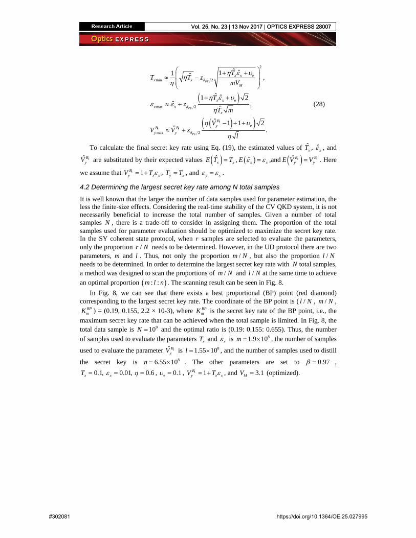
It is well known that the larger the number of data samples used for parameter estimation, the less the finite-size effects. Considering the real-time stability of the CV QKD system, it is not necessarily beneficial to increase the total number of samples. Given a number of total samples N , there is a trade-off to consider in assigning them. The proportion of the total samples used for parameter evaluation should be optimized to maximize the secret key rate. In the SY coherent state protocol, when r samples are selected to evaluate the parameters, only the proportion /r N needs to be determined. However, in the UD protocol there are two parameters, m and l . Thus, not only the proportion /m N , but also the proportion /l N needs to be determined. In order to determine the largest secret key rate with N total samples, a method was designed to scan the proportions of /m N and /l N at the same time to achieve an optimal proportion ( ): :m l n . The scanning result can be seen in Fig. 8.

In Fig. 8, we can see that there exists a best proportional (BP) point (red diamond) corresponding to the largest secret key rate. The coordinate of the BP point is ( /l N , /m N ,

BPmK ) = (0.19, 0.155, 2.2 × 10-3), where BP

mK is the secret key rate of the BP point, i.e., the maximum secret key rate that can be achieved when the total sample is limited. In Fig. 8, the total data sample is 910N = and the optimal ratio is (0.19: 0.155: 0.655). Thus, the number of samples used to evaluate the parameters xT and xε is 81.9 10m = × , the number of samples

used to evaluate the parameter 1ˆ ByV is 81.55 10l = × , and the number of samples used to distill

the secret key is 86.55 10n = × . The other parameters are set to 0.97β = , 0.1,xT = 0.01,xε = 0.6η = , e 0.1υ = , 1 1B

y x xV T ε= + , and 3.1MV = (optimized).


#302081 https://doi.org/10.1364/OE.25.027995


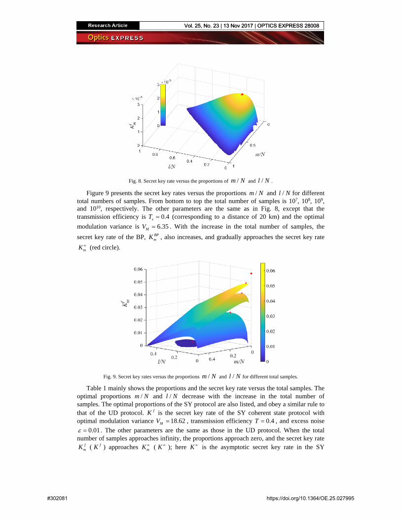
Fig. 8. Secret key rate versus the proportions of /m N and /l N .

Figure 9 presents the secret key rates versus the proportions /m N and /l N for different total numbers of samples. From bottom to top the total number of samples is 107, 108, 109, and 1010, respectively. The other parameters are the same as in Fig. 8, except that the transmission efficiency is 0.4xT = (corresponding to a distance of 20 km) and the optimal modulation variance is 6.35MV = . With the increase in the total number of samples, the secret key rate of the BP, BP

mK , also increases, and gradually approaches the secret key rate

mK ∞ (red circle).

Fig. 9. Secret key rates versus the proportions /m N and /l N for different total samples.

Table 1 mainly shows the proportions and the secret key rate versus the total samples. The optimal proportions /m N and /l N decrease with the increase in the total number of samples. The optimal proportions of the SY protocol are also listed, and obey a similar rule to that of the UD protocol. fK is the secret key rate of the SY coherent state protocol with optimal modulation variance 18.62MV = , transmission efficiency 0.4T = , and excess noise

0.01ε = . The other parameters are the same as those in the UD protocol. When the total number of samples approaches infinity, the proportions approach zero, and the secret key rate

fmK ( fK ) approaches mK ∞ ( K ∞ ); here K ∞ is the asymptotic secret key rate in the SY


#302081 https://doi.org/10.1364/OE.25.027995


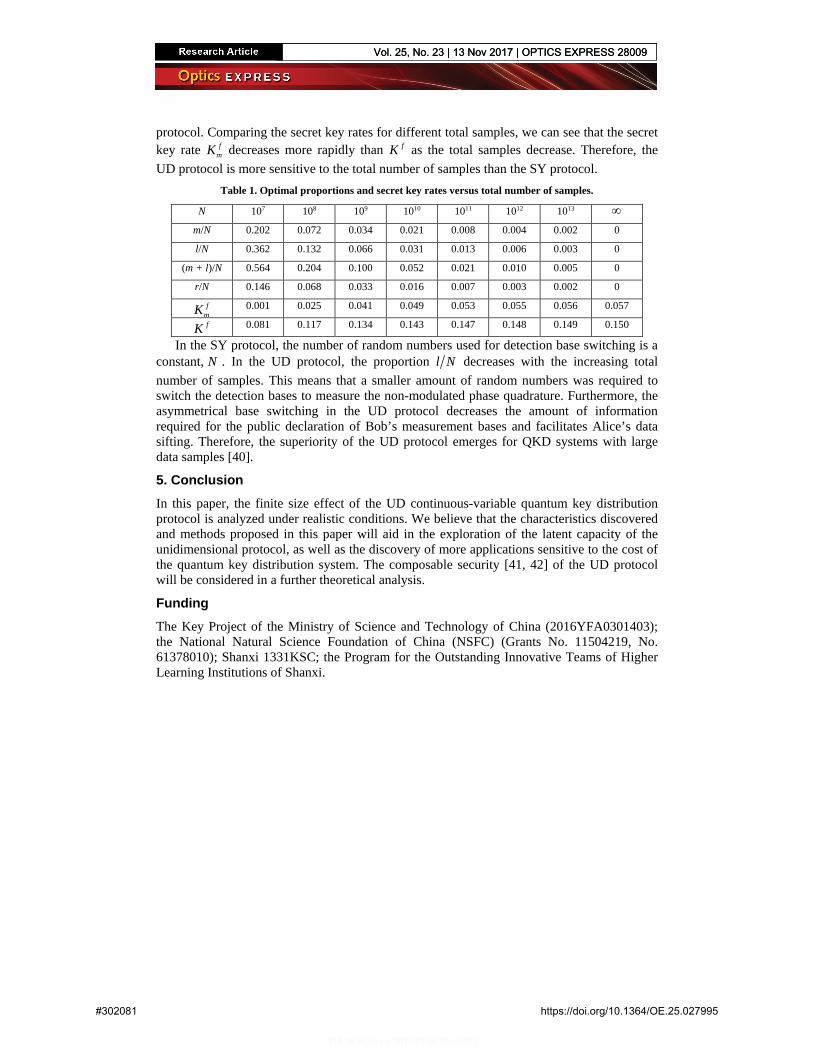
protocol. Comparing the secret key rates for different total samples, we can see that the secret key rate f

mK decreases more rapidly than fK as the total samples decrease. Therefore, the UD protocol is more sensitive to the total number of samples than the SY protocol.

Table 1. Optimal proportions and secret key rates versus total number of samples.

N 107 108 109 1010 1011 1012 1013 ∞m/N 0.202 0.072 0.034 0.021 0.008 0.004 0.002 0

l/N 0.362 0.132 0.066 0.031 0.013 0.006 0.003 0

(m + l)/N 0.564 0.204 0.100 0.052 0.021 0.010 0.005 0

r/N 0.146 0.068 0.033 0.016 0.007 0.003 0.002 0

fmK 0.001 0.025 0.041 0.049 0.053 0.055 0.056 0.057

fK 0.081 0.117 0.134 0.143 0.147 0.148 0.149 0.150

In the SY protocol, the number of random numbers used for detection base switching is a constant, N . In the UD protocol, the proportion l N decreases with the increasing total number of samples. This means that a smaller amount of random numbers was required to switch the detection bases to measure the non-modulated phase quadrature. Furthermore, the asymmetrical base switching in the UD protocol decreases the amount of information required for the public declaration of Bob’s measurement bases and facilitates Alice’s data sifting. Therefore, the superiority of the UD protocol emerges for QKD systems with large data samples [40].

5. ConclusionIn this paper, the finite size effect of the UD continuous-variable quantum key distribution protocol is analyzed under realistic conditions. We believe that the characteristics discovered and methods proposed in this paper will aid in the exploration of the latent capacity of the unidimensional protocol, as well as the discovery of more applications sensitive to the cost of the quantum key distribution system. The composable security [41, 42] of the UD protocol will be considered in a further theoretical analysis.

Funding The Key Project of the Ministry of Science and Technology of China (2016YFA0301403); the National Natural Science Foundation of China (NSFC) (Grants No. 11504219, No. 61378010); Shanxi 1331KSC; the Program for the Outstanding Innovative Teams of Higher Learning Institutions of Shanxi.


#302081 https://doi.org/10.1364/OE.25.027995


Documents

Finite-size analysis of unidimensional continuous-variable ... Express.25(23... · Finite-size analysis of unidimensional continuous -variable quantum key ... J. Cerf, and P . Grangier