Embed Size (px)
Citation preview
From Unidimensional to MultidimensionalInequality, Welfare and Poverty Measurement.
Claudio ZoliDepartment of EconomicsUniversity of Verona, Italy∗
January 2009Winter School on "Inequality and Welfare Theory", Canazei
Abstract
In this handout we review results concerning representation of partial or-ders via stochastic orders and investigate their applications to some classesof stochastic dominance conditions applied in inequality, poverty and welfaremeasurement. The results obtained in an unidimensional framework are ex-tended to multidimensional analysis. In particular we provide an overviewof the main issues concerning aggregation of multidimensional distributionsinto synthetic indicators as the Human Development Index or Social WelfareFunctions. Moreover we explore the potential for multidimensional evalua-tions based on the partial orders induced by different criteria of majorization.The lecture is divided into 4 parts: (i) an introduction to basic results con-cerning unidimensional evaluations of inequality, welfare and poverty (ii) anillustration of the problems of aggregation of evaluations when applied in themultidimensional context where individuals exhibit various attributes, (iii) thediscussion of the potentials and limits of the application of generalizations ofthe majorization approach to comparisons of multidimensional distributions(iv) a brief overview of some results on multidimensional stochastic orders.
∗Claudio Zoli, Dipartimento di Scienze Economiche, Università di Verona, Viale dell’Università4, 37129-Verona, Italy. E-MAIL: [email protected]
1
Contents
1 Introduction . . . . . . . . . . . . . . . . . . . . . . . . . . . . . . . . . . . 31.0.1 Aims of the lecture . . . . . . . . . . . . . . . . . . . . . . . . 4
1.1 Unidimensional/Multidimensional set up. . . . . . . . . . . . . . . . . 52 The Unidimensional case . . . . . . . . . . . . . . . . . . . . . . . . . . . . 6
2.0.1 Making use of distribution functions . . . . . . . . . . . . . . 62.1 How to rank distributions? . . . . . . . . . . . . . . . . . . . . . . . . 8
2.1.1 Stochastic orders . . . . . . . . . . . . . . . . . . . . . . . . . 82.2 Implementing stochastic orders: . . . . . . . . . . . . . . . . . . . . . 9
2.2.1 Comparison Tests . . . . . . . . . . . . . . . . . . . . . . . . . 92.2.2 Stochastic dominance conditions . . . . . . . . . . . . . . . . . 122.2.3 Stochastic Orders and Stochastic Dominance: Integral Stochas-
tic orders . . . . . . . . . . . . . . . . . . . . . . . . . . . . . 132.2.4 Stochastic Orders and Stochastic Dominance: Dual linear rank-
dependent stochastic orders . . . . . . . . . . . . . . . . . . . 152.3 Relation with more general results on unidimensional inequality and
welfare . . . . . . . . . . . . . . . . . . . . . . . . . . . . . . . . . . . 162.3.1 Basic properties: . . . . . . . . . . . . . . . . . . . . . . . . . 162.3.2 Links between Inequality & Welfare . . . . . . . . . . . . . . . 17
2.4 Poverty Evaluations . . . . . . . . . . . . . . . . . . . . . . . . . . . . 183 Multidimensional Case . . . . . . . . . . . . . . . . . . . . . . . . . . . . . 203.1 Consistency in Aggregation . . . . . . . . . . . . . . . . . . . . . . . 20
3.1.1 Consistent iterative aggregation . . . . . . . . . . . . . . . . . 213.1.2 A result by Dutta et al. (2003): . . . . . . . . . . . . . . . . . 213.1.3 Possible alternative solutions . . . . . . . . . . . . . . . . . . . 23
4 Multidimensional orders . . . . . . . . . . . . . . . . . . . . . . . . . . . . 284.1 Multidimensional Majorization . . . . . . . . . . . . . . . . . . . . . . 29
4.1.1 Relation with Progressive (Pigou Dalton) transfers . . . . . . 304.1.2 Tests for Multidimensional Majorization... . . . . . . . . . . . 324.1.3 Lift Zonoid and Lorenz Zonoid (by Koshevoy & Mosler) . . . . 33
4.2 Multidimensional Stochastic orders . . . . . . . . . . . . . . . . . . . 385 Suggested Readings . . . . . . . . . . . . . . . . . . . . . . . . . . . . . . . 42
2
1 Introduction
When comparing income distributions in terms of inequality, the most common tooladopted in applied works in the Lorenz curve. Comparisons made in terms of Lorenzcurves account for heterogeneity of views of policy makers or evaluators about thedegree of inequality aversion to adopt in the evaluation. It is indeed well knownthat if a Lorenz curve of a distribution is above the one of another distribution theninequality will be evaluated as lower for the former compared to the latter by a set ofinequality indices. A source of “discomfort” in applying the concept of dominance interms of the Lorenz curve relies instead on the fact that it induces a partial order, thatis, not all distributions can be unanimously compared since it is possible that for somedistributions the Lorenz curves intersect. The analysis of the dual aspect of “lackof completeness” and “unanimity of evaluations” is one of the issues explored in thefirst part of this lecture. We review results on the literature on “stochastic orders”i.e. orders of distributions based on unanimous dominance in terms of family ofevaluation functions and investigate their properties and their application to welfare,inequality and poverty measurement.1
The first part of the lecture will focus on the analysis of unidimensional distri-butions, e.g. income or consumption vectors of a given population. However themost interesting questions arise when facing comparisons based on multidimensionaldistributions, where for instance also education, health, or endowment of bundles ofgoods are taken into account. There exist therefore two different ways to approachthe multidimensional problem, the first one makes use of appropriate procedures toembody all information within an unique money metric indicator (e.g. equivalencescales or calculating budget income). Within this framework the different opinionsconcerning the aggregating procedures could be taken into account and partial rank-ing criteria could be specified in order to be consistent with a given range of admissibleaggregating functions.From the second point of view, inequality, as well as poverty and welfare, are
explicitly considered as multidimensional phenomena. Therefore the domain of theevaluation process is left multidimensional and ranking criteria are specified overthe set of all variables. Within this second framework it becomes natural to firstinvestigate whether it is more informative to focus first on the distribution of each at-tributes across the individuals as done by the Human Development Index or consideras a starting point the aggregation of each attribute per individual identifying the adistribution of utilities or individual indicators of well being. In the second part ofthe lecture we explore results on consistent aggregation obtained following these two
1Note that in what follows:% denotes a binary relation over a set of alternative,> denotes a stochastic order over distribution or random variables,< denotes a stochastic dominance condition on distributions or random variables, while≥ denotes the usual inequality symbol.
3
procedures highlighting the implications for many indices currently adopted in theliterature. Then we move to the more demanding quest of focussing on comparisonsthat use information on the whole matrix without filtering it through any interme-diate aggregation. This second approach is based on the concept of majorization[see Marshall and Olkin, 1974] that extends to the multivariate case the machineryapplied in the univariate case to obtain the Lorenz dominance criterion. A numberof critical issues arise in the multidimensional context and various criteria of domi-nance can be adopted. We will explore some of then and then we will get back to thestochastic orders framework illustrating some multidimensional results deriver in thestatistics/probability and decision theory literature.The structure of the lecture can be divide into 4 parts: (i) an introduction to basic
results concerning unidimensional evaluations of inequality, welfare and poverty (ii)an illustration of the problems of aggregation of evaluations when applied in the mul-tidimensional context where individuals exhibit various attributes, (iii) the discussionof the potentials and limits of the application of generalizations of the majorizationapproach to comparisons of multidimensional distributions (iv) a brief overview ofsome results on multidimensional stochastic orders. Each one of these parts can beaddressed almost separately, this is particularly the case for the distinction betweenthe unidimensional analysis (part (i)) and the multidimensional case (parts (ii), (iii),(iv)).
1.0.1 Aims of the lecture
Overview of selected issues underlying the theory of measurement of inequality, wel-fare, poverty and well being.Two broad perspectives:
1. Unidimensional: Individuals/households are homogeneous in all ethically rel-evant characteristics except consumption or income.
2. Multidimensional: heterogeneous individuals exhibiting differences in a num-ber of "characteristics" (transferable and non transferable) e.g. income, health,housing, bundles of goods, education, household size, level of needs.....
A number of interrelated perspectives of evaluation can be taken into account:
1. Inequality (focuses on dispersions across agents, i.e. considers how the cake(e.g. GDP) is shared in the population),
2. Welfare (takes into account also the size of the cake, for instance each agentcan improve her situation in a world where the per-capita income is larger eventhough is more unequally distributed)
3. Poverty (focuses on deprived agents, size and dispersion matters but the concernis only for those deprived, e.g. with income below the poverty line)
4
4. Well being: multidimensional perspective focussing on size and dispersion. Amore unequal distribution in one attribute across the population might com-pensate for the unequal distributions in other attribute, i.e. it is not always thecase that an increase in inequality in one attribute reduces society well being.This is clearly the case if agents that are better of in the distribution of someattributes continue to be advantaged by the distribution of other attributes,that is if the correlation between the distribution of the attributes is positive.
Evaluations can be formalized through:
1. Complete rankings, i.e. indices or welfare functions, or
2. Partial rankings, i.e. identification of dominance conditions that may not rankany pair of distribution, this is the case for instance for the Lorenz dominancecondition based on comparisons of Lorenz curves. Dominance occurs in this caseif the Lorenz curve of one distribution is above the one of another distribution,if these curve intersect the dominance test is not conclusive.
Our Concern is
• To provide some intuitions on the interrelations between the various conceptsin the unidimensional case and then move to the MORE INTERESTING mul-tidimensional case.........
1.1 Unidimensional/Multidimensional set up.
Consider:
• n homogeneous individuals i = 1, 2, ..., n ≥ 2• Rn
+ : n−dimensional (n) vector of non-negative (+) real numbers (R)• d ≥ 1 characteristics, goods, attributes, attainments (e.g. income) j = 1, 2, 3, ..., d• Distribution X ∈ Rn×d
+
X =
x11 ... ... x1(d−1) x1dx21 x22 ... ... x2d... · ...
xn1 xn2 ... ... xnd
Rows identify individuals/households and columns are associated with attributesor characteristics
5
• x.j distribution of attribute j across all individuals, xi. distribution of all theattributes for individual i, x ∈ Rd
+ generic vector of values for the attributes,or x ∈ Rn
+ generic vector of distribution for n individuals.
• FX(x) or F (x)cumulative distribution function: percentage of individuals withincome not higher than x (unidimensional case) or in general FX(x) percentageof individuals whose vector of attributes is not larger than x ∈ Rd
+ (multidi-mensional case)
• µ(x.j) average of distribution x.j of attribute j (e.g. income) :
µ(x.j) =Xn
i=1xij/n.
• x.j ordered distribution of attribute j: x(1)j ≤ x(2)j ≤ ..x(i)j... ≤ x(n)j
• I(X) Inequality index, I : Rn×d+ → R [function from the set of all admissible
distributions Rn×d+ to (→) the set of real numbers (R)]
• W (X) Social Evaluation Function (SEF) it is defined over incomesW : Rn×d+ →
R
• zj > 0 poverty line for attribute j, z ∈ Rd+ vector of poverty lines for each
attribute.
• P (X,z) Poverty index, P : Rn×d+ × Rd
++ → R [function from the set of alladmissible distributions (Rn×d
+ ) and from the set of positive values (R++) ofany poverty line zj , to (→) the set of real numbers (R)]
2 The Unidimensional case
2.0.1 Making use of distribution functions
As a starting point one might analyse distributions making use of statistical graphicaltools. For instance the primitive tool both for continuous or discrete distributionscan be the Cumulative Distribution Function. It can also be specified [later on] formultidimensional distributions.
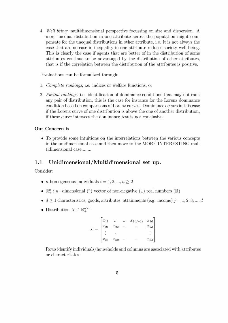
Definition 2.1 (Cumulative Distribution Function) F : R+ → [0, 1] FunctionF (x) plotting the proportion of income units within the population with income atmost x.
6
C.d.f. Fx(x) for x = (10, 20, 30, 30, 60)
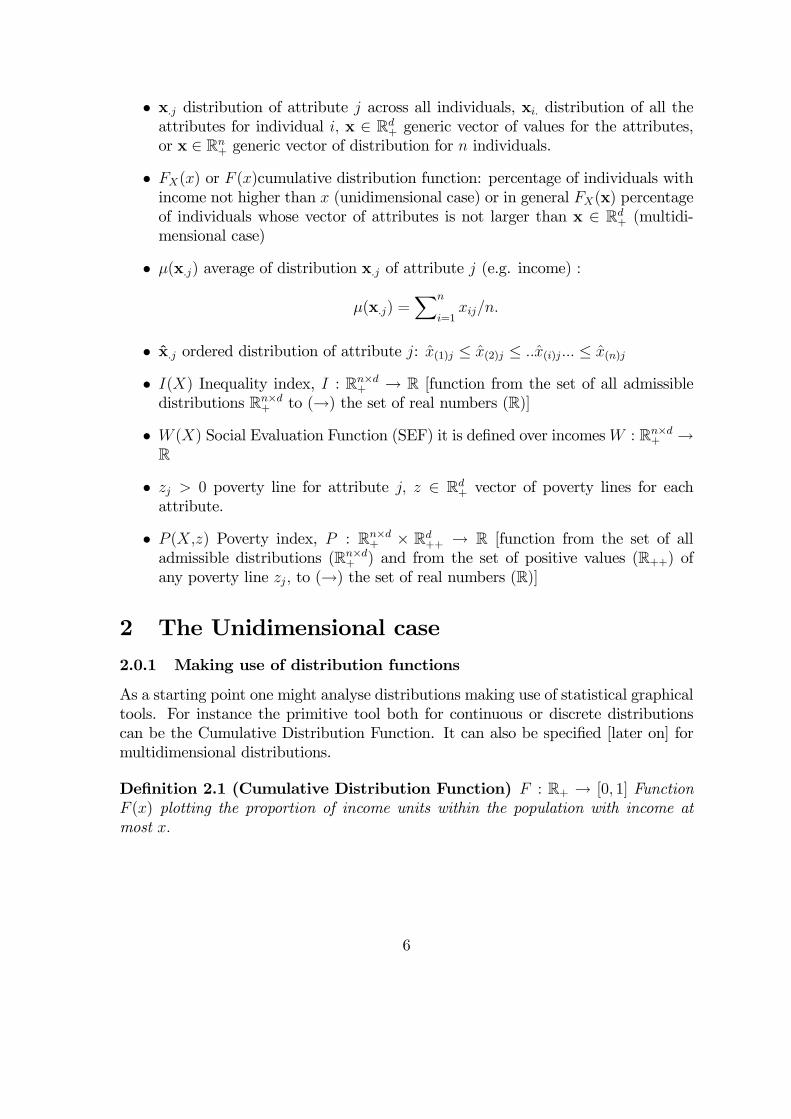
It is possible to use the information in the C.d.f. in order to construct a dualrepresentation. Reversing the graphs we get the Pen’s Parade (or inverse distribu-tion function): The parade of all the incomes in increasing order weighted by thepercentage of individuals to whom these incomes belong (sample weight).
Definition 2.2 (Inverse Distribution Function) F−1 : [0, 1] → R+. FunctionF−1(p) plotting the income level corresponding to the pth quantile of the populationonce incomes are ranked in ascending order, i.e. left continuous inverse distribution:
F−1(p) = inf{x ∈ R+ : F (x) ≥ p}.
Inv.d.f. F−1x (p) for x = (10, 20, 30, 30, 60)
7
2.1 How to rank distributions?
2.1.1 Stochastic orders
We consider the issue of unanimous dominance for a set of indices or evaluationfunctions. We focus on two broad families of functionals. commonly adopted ininequality, welfare and risk analysis.
Definition 2.3 Additively decomposable order >U
X > U Y
⇔Wu(X) =
ZRu(x)dFX(x) ≥
ZRu(x)dFY (x) =Wu(Y ), ∀u ∈ U
alternatively
1
n
nXi=1
u(xi) ≥ 1
n
nXi=1
u(yi) ∀u ∈ U
The key property of the utilitarian/expected utility representation is Indepen-dence:
Definition 2.4 (Independence) Joining (or mixing) two distributions (or popu-lations of individuals) with a third distribution (another group of individuals) theranking of the new distributions obtained is consistent with the ranking of the formertwo distributions: Wu(X,Z) ≥Wu(Y,Z) if and only if Wu(X) ≥Wu(Y ).
The realization of each individual is transformed according to the function u whilehis/her weight in the final formula enters linearly.Next family is dual w.r.t. the previous and is based on weighted averages of the
realizations, where weight depends on the ranking of each realization.
Definition 2.5 Rank dependent (dual) order >V
X > V Y
⇔Wv(X) =
Z 1
0
v(p) · F−1X (p)dp ≥Z 1
0
v(p) · F−1Y (p)dp =Wv(Y ) ∀v ∈ Valternatively
1
n
nXi=1
vi · x(i) ≥ 1
n
nXi=1
vi · y(i) ∀v ∈ V
where vi ≥ 0; x(1) ≤ x(2) ≤ ... ≤ x(i) ≤ ... ≤ x(n)
8
The key property this rank dependent/generalized Gini representation is ComonotonicIndependence:
Definition 2.6 (Comonotonic Independence) When adding to two distributions(i.e. distributions of labour income) a third distribution (e.g. a distribution of capitalincome) that is comonotonic w.r.t. the former two (i.e. capital income is ranked inthe same order as the labour incomes in the former distributions) then the two newdistributions obtained is consistent with the ranking of the former two distributions:Wv(X + Z) ≥Wv(Y + Z) if and only if Wv(X) ≥Wv(Y ).
The realization of each individual is considered linearly in the final evaluationwhile the individual weight in the final formula enters through vi according to his/herposition in the ranking of the attribute.
Remark 2.1 These criteria are partial orders i.e. they do not necessarily provide aclear-cut ranking. For some distributions the answer may not be conclusive this is thecase when for instance Wv(X) > Wv(Y ) for some v ∈ V but Wv0(X) < Wv0(Y ) forsome others v0 ∈ V
2.2 Implementing stochastic orders:
2.2.1 Comparison Tests
Consider X income distribution of finite mean µ(X) [or µX ], defined on a boundedsupport in R+.
• Is it possible to device tools that we can apply directly in order to test dominanceof one distribution over another?
The most common tools applied in inequality analysis to compare income distri-butions are indeed the partial orders induced by the stochastic dominance conditions(direct and inverse).For instance typical dominance conditions are:
Definition 2.7 (Lorenz Dominance) Define the Lorenz curve for X:
LX(p) :=
Z p
0
F−1X (t)
µ(X)dt.
Income profile X Lorenz dominates income profile Y, X <L Y, if and only if
LX(p) ≥ LY (p) for all p ∈ [0, 1] .
9
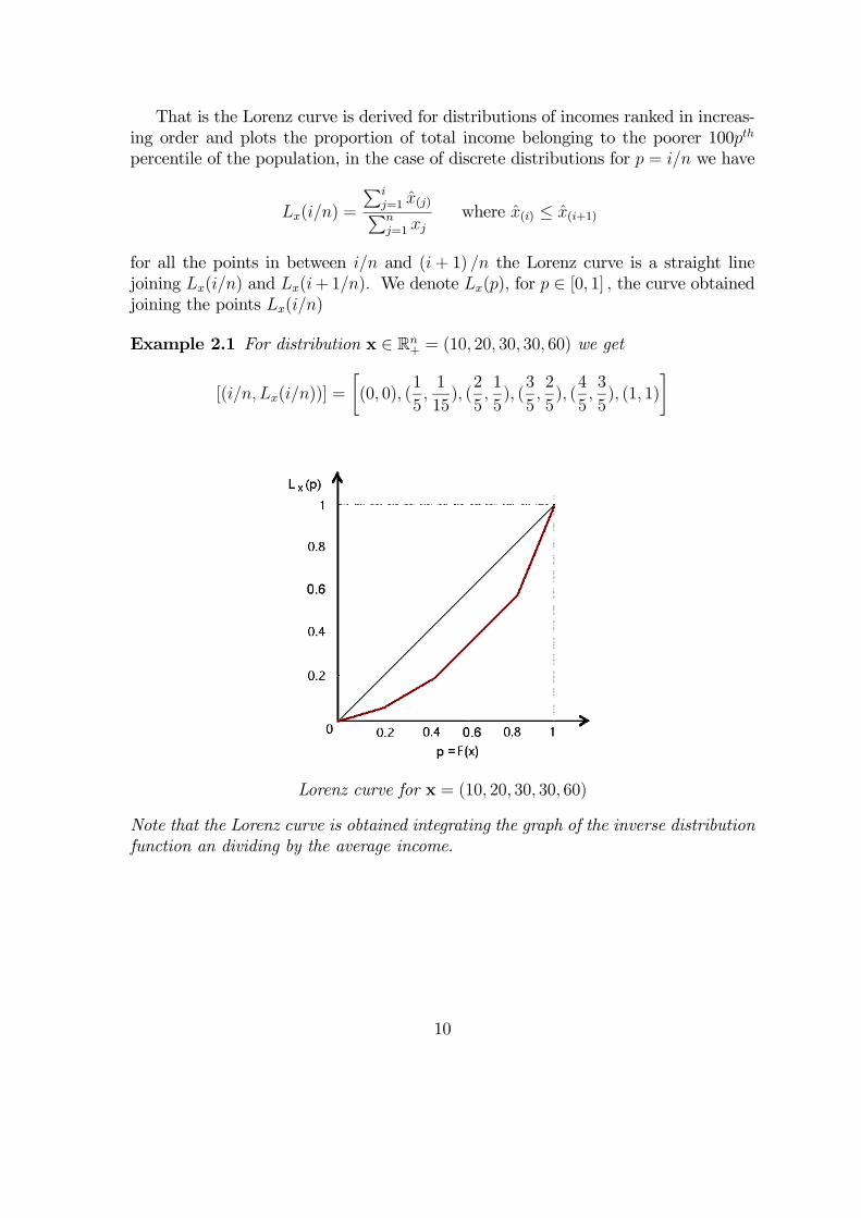
That is the Lorenz curve is derived for distributions of incomes ranked in increas-ing order and plots the proportion of total income belonging to the poorer 100pth
percentile of the population, in the case of discrete distributions for p = i/n we have
Lx(i/n) =
Pij=1 x(j)Pnj=1 xj
where x(i) ≤ x(i+1)
for all the points in between i/n and (i+ 1) /n the Lorenz curve is a straight linejoining Lx(i/n) and Lx(i+1/n). We denote Lx(p), for p ∈ [0, 1] , the curve obtainedjoining the points Lx(i/n)
Example 2.1 For distribution x ∈ Rn+ = (10, 20, 30, 30, 60) we get
[(i/n, Lx(i/n))] =
·(0, 0), (
1
5,1
15), (2
5,1
5), (3
5,2
5), (4
5,3
5), (1, 1)
¸
Lorenz curve for x = (10, 20, 30, 30, 60)
Note that the Lorenz curve is obtained integrating the graph of the inverse distributionfunction an dividing by the average income.
10
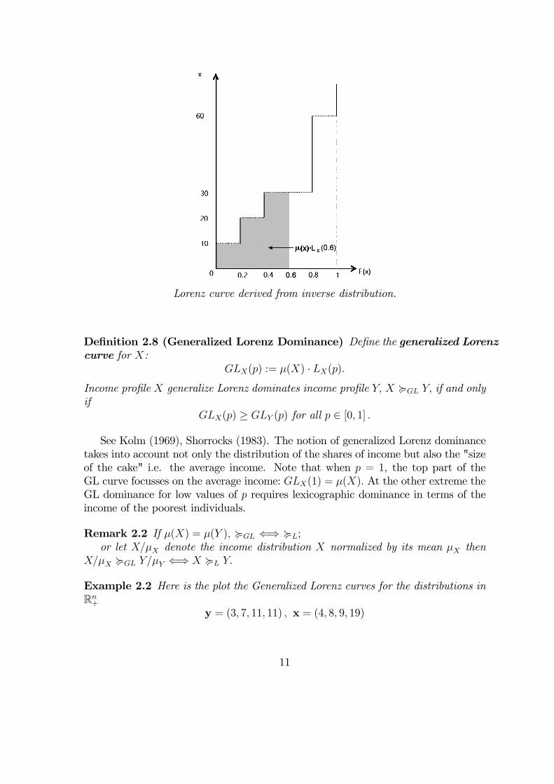
Lorenz curve derived from inverse distribution.
Definition 2.8 (Generalized Lorenz Dominance) Define the generalized Lorenzcurve for X:
GLX(p) := µ(X) · LX(p).
Income profile X generalize Lorenz dominates income profile Y, X <GL Y, if and onlyif
GLX(p) ≥ GLY (p) for all p ∈ [0, 1] .
See Kolm (1969), Shorrocks (1983). The notion of generalized Lorenz dominancetakes into account not only the distribution of the shares of income but also the "sizeof the cake" i.e. the average income. Note that when p = 1, the top part of theGL curve focusses on the average income: GLX(1) = µ(X). At the other extreme theGL dominance for low values of p requires lexicographic dominance in terms of theincome of the poorest individuals.
Remark 2.2 If µ(X) = µ(Y ), <GL ⇐⇒ <L;or let X/µX denote the income distribution X normalized by its mean µX then
X/µX <GL Y/µY ⇐⇒ X <L Y.
Example 2.2 Here is the plot the Generalized Lorenz curves for the distributions inRn+
y = (3, 7, 11, 11) , x = (4, 8, 9, 19)
11
Generalized Lorenz Curves for y = (3, 7, 11, 11) , x = (4, 8, 9, 19)
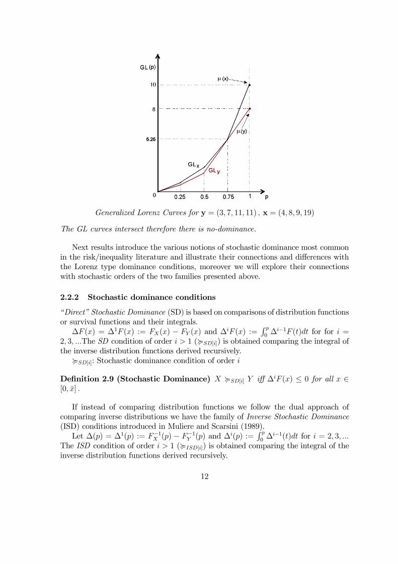
The GL curves intersect therefore there is no-dominance.
Next results introduce the various notions of stochastic dominance most commonin the risk/inequality literature and illustrate their connections and differences withthe Lorenz type dominance conditions, moreover we will explore their connectionswith stochastic orders of the two families presented above.
2.2.2 Stochastic dominance conditions
“Direct” Stochastic Dominance (SD) is based on comparisons of distribution functionsor survival functions and their integrals.
∆F (x) = ∆1F (x) := FX(x) − FY (x) and ∆iF (x) :=R p0∆i−1F (t)dt for for i =
2, 3, ...The SD condition of order i > 1 (<SD[i]) is obtained comparing the integral ofthe inverse distribution functions derived recursively.<SD[i]: Stochastic dominance condition of order i
Definition 2.9 (Stochastic Dominance) X <SD[i] Y iff ∆iF (x) ≤ 0 for all x ∈[0, x] .
If instead of comparing distribution functions we follow the dual approach ofcomparing inverse distributions we have the family of Inverse Stochastic Dominance(ISD) conditions introduced in Muliere and Scarsini (1989).Let ∆(p) = ∆1(p) := F−1X (p) − F−1Y (p) and ∆i(p) :=
R p0∆i−1(t)dt for i = 2, 3, ...
The ISD condition of order i > 1 (<ISD[i]) is obtained comparing the integral of theinverse distribution functions derived recursively.
12
Definition 2.10 (Inverse Stochastic Dominance) X <ISD[i] Y iff ∆i(p) ≥ 0 forall p ∈ [0, 1] .Remark 2.3 Note that X <ISD[1] Y denotes rank dominance (Saposnik, 1981) whileX <ISD[2] Y denotes generalized Lorenz dominance.
Remark 2.4 X <SD[i] Y =⇒ X <SD[i+1] Y ; X <ISD[i] Y =⇒ X <ISD[i+1] Y ;
Remark 2.5 X <SD[i] Y ⇐⇒ X <ISD[i+1] Y for i = 1, 2.X <SD[i] Y 6=⇒6⇐= X <ISD[i+1] Y for i = 3, 4, 5....
2.2.3 Stochastic Orders and Stochastic Dominance: Integral Stochasticorders
Consider random variables (income profiles)X defined on [0, x] the Integral StochasticOrder (Additively decomposable) can be specified as
X >U Y ⇔Z x
0
u(x)d[∆F (x)] ≥ 0 ∀u ∈ U . (1)
In order to investigate the relationships between stochastic orders >U and stochas-tic dominance <SD[i] we focus on “nested” classes of utility functions u : [0, x]→ R.
U1 := {u continuous and non-decreasing}.U2 := {u ∈ U1 : concave}.U3 := {u ∈ U2 : u0 convex}.
Remark 2.6 Pα(X, z) =R z0(z−x)αdFX is the absolute version of Foster, Greer and
Thorbecke (1984) poverty index [FGT] for α ≥ 0, where z > 0 denotes the povertyline.For discrete distributions ranked in increasing order x, with q individuals not above
the poverty line z the relative version of FGT index is P rα = z−α · Pα :
P rα(x,z) =
1
n
Xq
i=1
µz − x(i)
z
¶α
for α ≥ 0,
Thus
P0(x,z) =q
n, Head count ratio
P1(x,z) =1
n
Xq
i=1
¡z − x(i)
¢P2(x,z) =
1
n
Xq
i=1
¡z − x(i)
¢2.
Dominance in terms of poverty indices for any poverty line can be related to stochasticdominance conditions.
13
Theorem 2.1 (Foster-Shorrocks (1988); Fishburn (1976)) Let n ∈ {1, 2, 3}.The following statements are equivalent:(i) Pk−1(X,z) ≤ Pk−1(X,z) for all poverty lines z ≤ x.(ii) X <SD[k] Y .
See also Dardanoni and Lambert (1988) for n = 3. Less poverty as evaluatedaccording to the poverty index Pn−1 and for all possible poverty lines coincides withstochastic dominance of order n.
Remark 2.7 Note that P0(X,x) = H(X, x) : the headcount of profile X evaluated atthe upper bound, i.e. the proportion of population with income not larger than x, thusP0(X,x) = 1 = P0(Y ,x).
P1(X,x) ≤ P1(Y ,x)⇐⇒ µ(X) ≥ µ(Y )If µ(X) = µ(Y ) then P2(X,x) ≤ P2(Y ,x) ⇐⇒ σ2(X) ≤ σ2(Y ) where σ2 denotes
the variance.
Next result clarifies a further relation between poverty and evaluations in term ofstochastic orders:
Theorem 2.2 Let k = 1, 2, 3, the following statements are equivalent:(i) X >Uk Y(ii) X <SD[k] Y [and µ(X) ≥ µ(Y ) for k = 3].
Concerning the role of variance it is also worth to point out that
Theorem 2.3 (Shorrocks-Foster (1987); Dardanoni-Lambert (1988)) If (a)∆2F (x) changes sign once, (b) µ(X) = µ(Y ) and (c) X dominates Y in terms ofLeximin, then X <SD[3] Y ⇐⇒ σ2(X) ≤ σ2(Y ).
Remark 2.8 (Inequality Comparisons) Concerning inequality comparisons basedon relative inequality indices (i.e. scale invariant indices) then all previous statements[except for <SD[1]] hold provided that income profiles X/µX and Y/µY are compared.Here we take the view that for distributions with equal means welfare dominance
implies a reduction in inequality, more precisely X/µX <SD[n] Y/µY means that Xshows less inequality than Y.Since X/µX and Y/µY exhibit the same mean equal to 1, then noticing that
X <SD[1] Y =⇒ µ(X) ≥ µ(Y ) it follows that either X/µX and Y/µY are not compa-rable according to <SD[1] or they induce the same distribution function and thereforethey are equivalent for all orders of stochastic dominance.
14
2.2.4 Stochastic Orders and Stochastic Dominance: Dual linear rank-dependent stochastic orders
We focus directly on the specification of the stochastic order based on weightingfunctions:
X > VY ⇔Z 1
0
v(p) · F−1X (p)dp ≥Z 1
0
v(p) · F−1Y (p)dp ∀v ∈ V
⇔Z 1
0
v(p) ·∆(p)dp ≥ 0 ∀v ∈ V (2)
Before moving to the selection of the classes of weighting functions V we recallsome parametric classes of SEFs, the class of S-Gini [single parameter] SEFs Ξ(δ; .)introduced in Donaldson and Weymark (1980, 1983) and Yitzhaki (1983). It is para-meterized by δ ≥ 1 and is obtained letting v(p) = δ(1− p)δ−1 that is
Ξ(δ;X) : = δ
Z 1
0
(1− p)δ−1F−1X (p)dp (3)
=
ZR+[1− FX(t)]
δ dt. (4)
Note that Ξ(0;Xp) = limδ→0 Ξ(δ;X) = F−1X (p); Ξ(1;X) = µ(X) while for δ = 2 weobtain the SEF associated with the Gini index G(.) i.e. Ξ(2;X) = µ(X) · [1−G(X)].That is
G(X) := 1− Ξ(2;X)
µ(X)=
Z 1
0
(2p− 1) · F−1X (p)
µ(X)dp.
We investigate the relationships between stochastic orders >V and inverse sto-chastic dominance <ISD[i] .We focus on “nested” classes of weighting functions v : [0, 1]→ R+ integrating to
1, where
V1 := {v ∈ L1([0, 1]) : v ≥ 0, andZ 1
0
v(t)dt = 1}V2 := {v ∈ V1 : v non-increasing}V3 := {v ∈ V2 : v convex}.
Definition 2.11 (Truncated income profiles Xp) Xp denotes the income profileX truncated at quantile p such that F−1Xp
(t) = F−1X (t · p).Then µ(Xp) is the incomplete mean of distribution X evaluated for the poorest p
fraction of individuals.
Theorem 2.4 (Maccheroni, Muliere, Zoli (2005)) Let k ∈ {1, 2, 3}. The fol-lowing statements are equivalent:(i) Ξ(k − 1;Xp) ≥ Ξ(k − 1;Yp) for all p ∈ [0, 1](ii) X <ISD[k] Y .
15
Inverse stochastic dominance of order n is equivalent to dominance for S-Giniindices where δ = n− 1 for distributions truncated at any p.Remark 2.9 (Zoli (1999)) An interesting case: k = 3;
X <ISD[3] Y ⇐⇒ µ(Xp)[1−G(Xp)] ≥ µ(Yp)[1−G(Yp)] for all p ∈ [0, 1].Note that if µ(X) = µ(Y ) then X <ISD[3] Y =⇒ G(X) ≤ G(Y ).
As a result we obtain as derived in Zoli (1999), Wang and Young (1998), andAaberge (2004)
Theorem 2.5 Let k = 1, 2, 3 the following statements are equivalent:(i) X >Vk Y(ii) X <ISD[k] Y [and µ(X) ≥ µ(Y ) for k = 3].
Concerning the role of the Gini index it is also worth to point out that
Theorem 2.6 (Zoli (1999)) If (a) ∆2(p) changes sign once, (b) µ(X) = µ(Y ) and(c) X dominates Y in terms of Leximin, then X <ISD[3] Y ⇐⇒ G(X) ≤ G(Y ).
2.3 Relation with more general results on unidimensionalinequality and welfare
We start with inequality indices that satisfy the following conditions:
• I(x) is continuous in xi : small changes in incomes do not lead to big changesin the value of the index.
• I(x) is normalized: that is I(µ, µ, .., µ) = 0.
2.3.1 Basic properties:
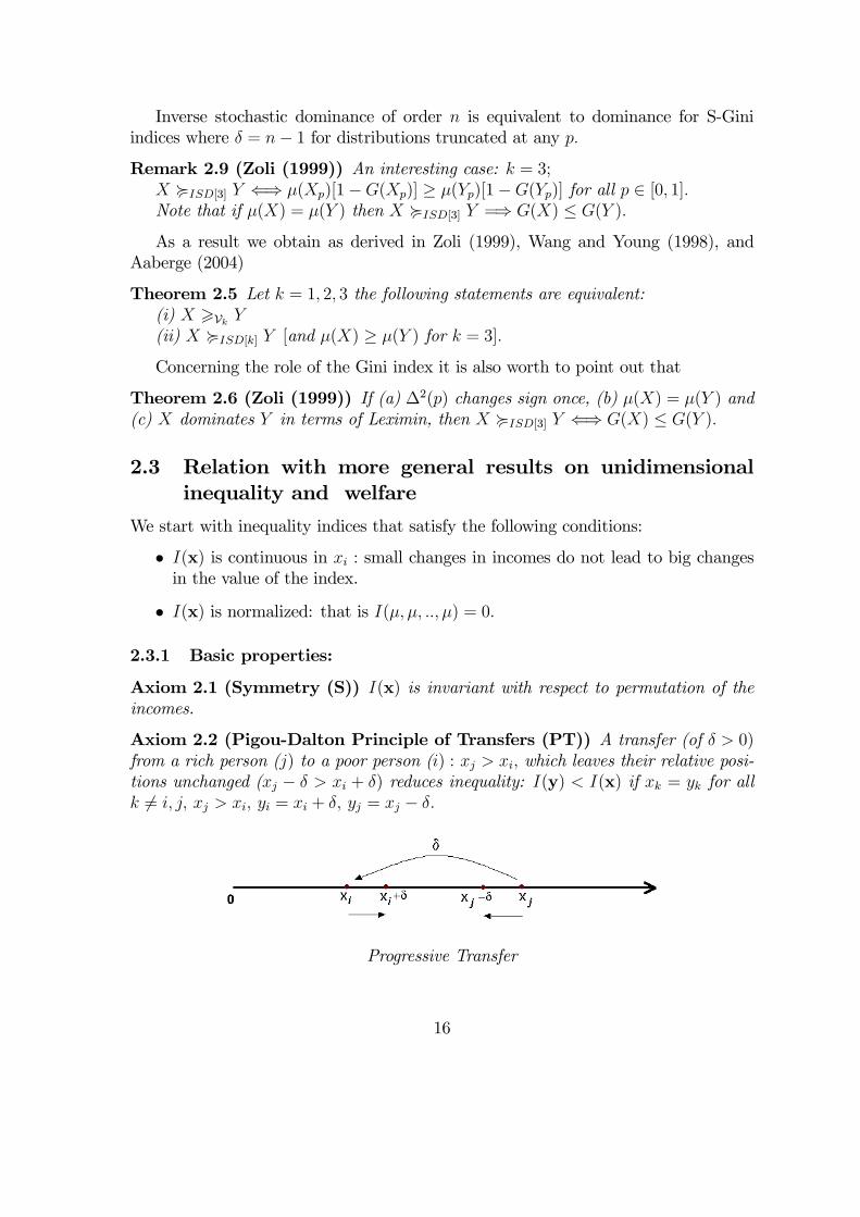
Axiom 2.1 (Symmetry (S)) I(x) is invariant with respect to permutation of theincomes.
Axiom 2.2 (Pigou-Dalton Principle of Transfers (PT)) A transfer (of δ > 0)from a rich person (j) to a poor person (i) : xj > xi, which leaves their relative posi-tions unchanged (xj − δ > xi + δ) reduces inequality: I(y) < I(x) if xk = yk for allk 6= i, j, xj > xi, yi = xi + δ, yj = xj − δ.
Progressive Transfer
16
Such a transfer is called: PROGRESSIVE TRANSFER (the inverse type of trans-fer, i.e. going in the opposite direction is called Regressive Transfer)
Axiom 2.3 (Relative Inequality (Rel)) Often called also Scale Invariance: I(x) =I(λx) for λ > 0.
Theorem 2.7 (Hardy, Littlewood & Polya 1934 (HL&P)) Consider a fixed num-ber of individuals n, let µ(x) = µ(y), the following statements are equivalent:
(1) For all k ≤ n,Pk
i=1 xi ≥Pk
i=1 yi with at least one strict inequality (>).
(2) x can be obtained from y through a finite sequence of progressive transfers.
(3) Let Wu(x) =Pn
i=1 u(xi) the Utilitarian Social Evaluation Function, Wu(x) >Wu(y) for all Wu(x) such that u(.) is increasing and strictly concave.
(4) Let Iφ(x) =Pn
i=1 φ(xi) the additive inequality index Iφ(x) < Iφ(y) for all Iφ(x)such that φ(.) is strictly convex.
Direct relation of HL&P theorem with results in term of inequality indices.
Theorem 2.8 (Dasgupta, Sen and Starret 1973) Let distributions x,y ∈ Rn+
and µ(x) = µ(y), the following statements are equivalent:1.a) I(x) < I(y) for all inequality indices I : Rn
+ → R satisfying Symmetry andPrinciple of Transfers (strictly S-Convex indices)2.a) x ÂL y
Extension to relative inequality comparisons of distributions with different meanincomes.
Theorem 2.9 (Foster 1985) Let x,y ∈ Rn+ the following statements are equivalent:
1) I(x) < I(y) for all inequality Relative indices I : Rn+ → R satisfying Symme-
try and Principle of Transfers2) x ÂL y.
2.3.2 Links between Inequality & Welfare
We consider Social Evaluation Function (SEF) W (x)
Definition 2.12 (Social Evaluation Function (SEF)) W : Rn+ → R is a SEF if
for every income distribution in X provides a welfare evaluation.
SEFs differ from Social Welfare Functions because they provide a welfare evalua-tion based on individuals’ income and not directly on individuals’ utility or well-being.
Axiom 2.4 (Inequality - Welfare Consistency (IWC)) If µ(x) = µ(y) then forall x,y ∈ Rn
+
I(x) ≤ I(y)⇔W (x) ≥W (y).
17
However the SEF should also be increasing in each individual income. As a result
Theorem 2.10 (Shorrocks (1983); Kolm (1969)) Let x,y ∈ Rn+ the following
statements are equivalent:(i) x ÂGL y(ii) W (x) > W (y) for all increasing SEFs W (x) satisfying Symmetry,and Prin-
ciple of Transfers.(iii) 1
n
Pni=1 u(xi) >
1n
Pni=1 u(yi) for all Average Utilitarian SEFs where u(.) is
increasing and strictly concave.
2.4 Poverty Evaluations
Note that for a given poverty line z > 0 poverty dominance conditions can be specifiedas integral stochastic orders, or a rank-dependent stochastic orders, respectively whenthe family of indices
Pp(X, z) =
Z z
0
p(x, z)dFX (5)
or
Pv(X, z) =
Z 1
0
v(p) · £z − F−1X (p)¤+dp (6)
are considered. The associated poverty stochastic orders >P can be specified as:
X > PU Y ⇔ Pp(X, z) ≤ Pp(Y, z) ∀ − p(x, z) = uz(x) ∈ U
⇔Z z
0
uz(x)dFX ≥Z z
0
uz(x)dFY ∀uz ∈ U
⇔Z z
0
uz(x)d∆F ≥ 0 ∀uz ∈ U (7)
Remark 2.10 Note that:(i) X >P
U1 Y ⇐⇒ X <SD[1] Y on [0, z](ii) X >P
U2 Y ⇐⇒ X <SD[2] Y on [0, z] and P0(X,z) = H(X, z) ≤ H(Y, z) =P0(Y ,z)
While for rank-dependent stochastic orders we have for [t]+ := max{t, 0}
X > PVY ⇔ Pv(X, z) ≤ Pv(Y, z) ∀v ∈ V
⇔Z 1
0
v(p) · £z − F−1X (p)¤+dp ≤
Z 1
0
v(p) · £z − F−1Y (p)¤+dp ∀v ∈ V
⇔Z 1
0
v(p) ·∆z(p)dp ≥ 0 ∀v ∈ V (8)
where ∆z(p) =£z − F−1Y (p)
¤+− £z − F−1X (p)
¤+.
18
Remark 2.11 Note that:(i) X >P
V1 Y ⇐⇒£z − F−1Y (p)
¤+≥ £z − F−1X (p)
¤+∀p ∈ [0, 1]
(ii) X >PV2 Y ⇐⇒
R p0
£z − F−1Y (p)
¤+dp ≥ R p
0
£z − F−1X (p)
¤+dp ∀p ∈ [0, 1]
Note that the integral condition in (ii) denotes dominance according to the ab-solute version (i.e. multiplied by the value of the poverty line z > 0) poverty depri-vation curve or absolute TIP curve (TIP stands for Three I’s of Poverty, because itcaptures the Incidence, Intensity and Inequality aspects of the poverty evaluation)derived in Spencer and Fisher (1992), Jenkins and Lambert (1997) and Shorrocks(1998).
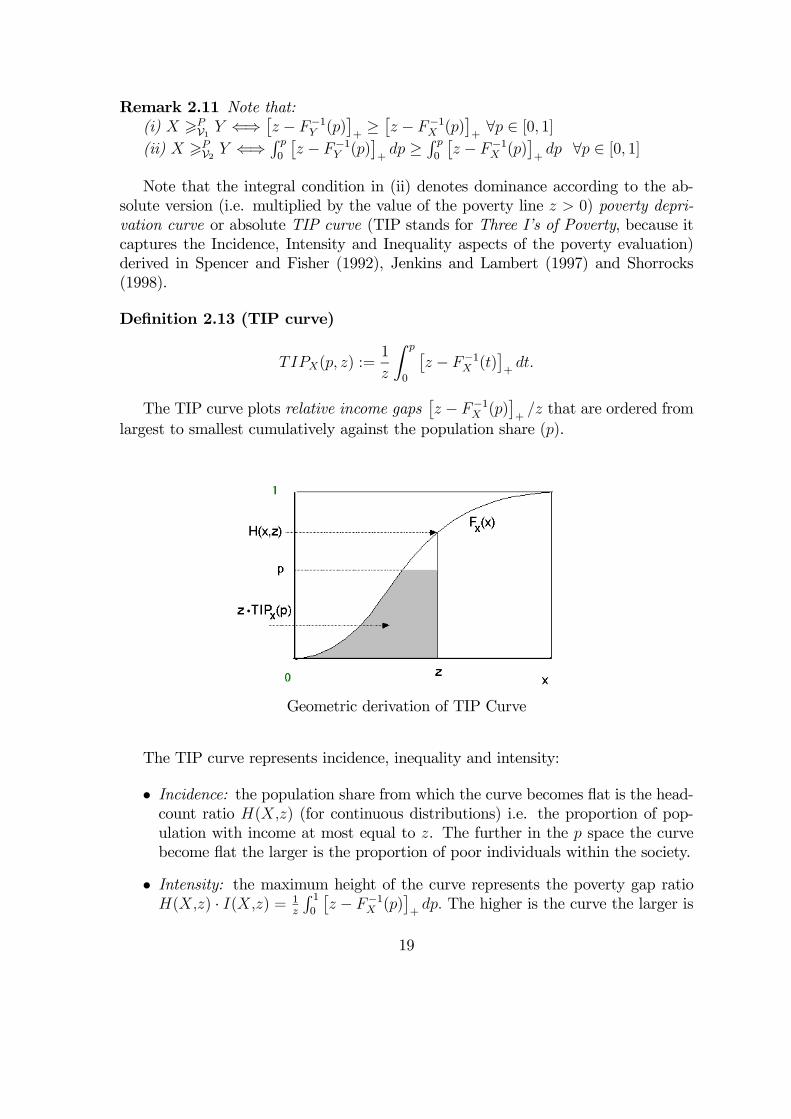
Definition 2.13 (TIP curve)
TIPX(p, z) :=1
z
Z p
0
£z − F−1X (t)
¤+dt.
The TIP curve plots relative income gaps£z − F−1X (p)
¤+/z that are ordered from
largest to smallest cumulatively against the population share (p).
Geometric derivation of TIP Curve
The TIP curve represents incidence, inequality and intensity:
• Incidence: the population share from which the curve becomes flat is the head-count ratio H(X,z) (for continuous distributions) i.e. the proportion of pop-ulation with income at most equal to z. The further in the p space the curvebecome flat the larger is the proportion of poor individuals within the society.
• Intensity: the maximum height of the curve represents the poverty gap ratioH(X,z) · I(X,z) = 1
z
R 10
£z − F−1X (p)
¤+dp. The higher is the curve the larger is
19
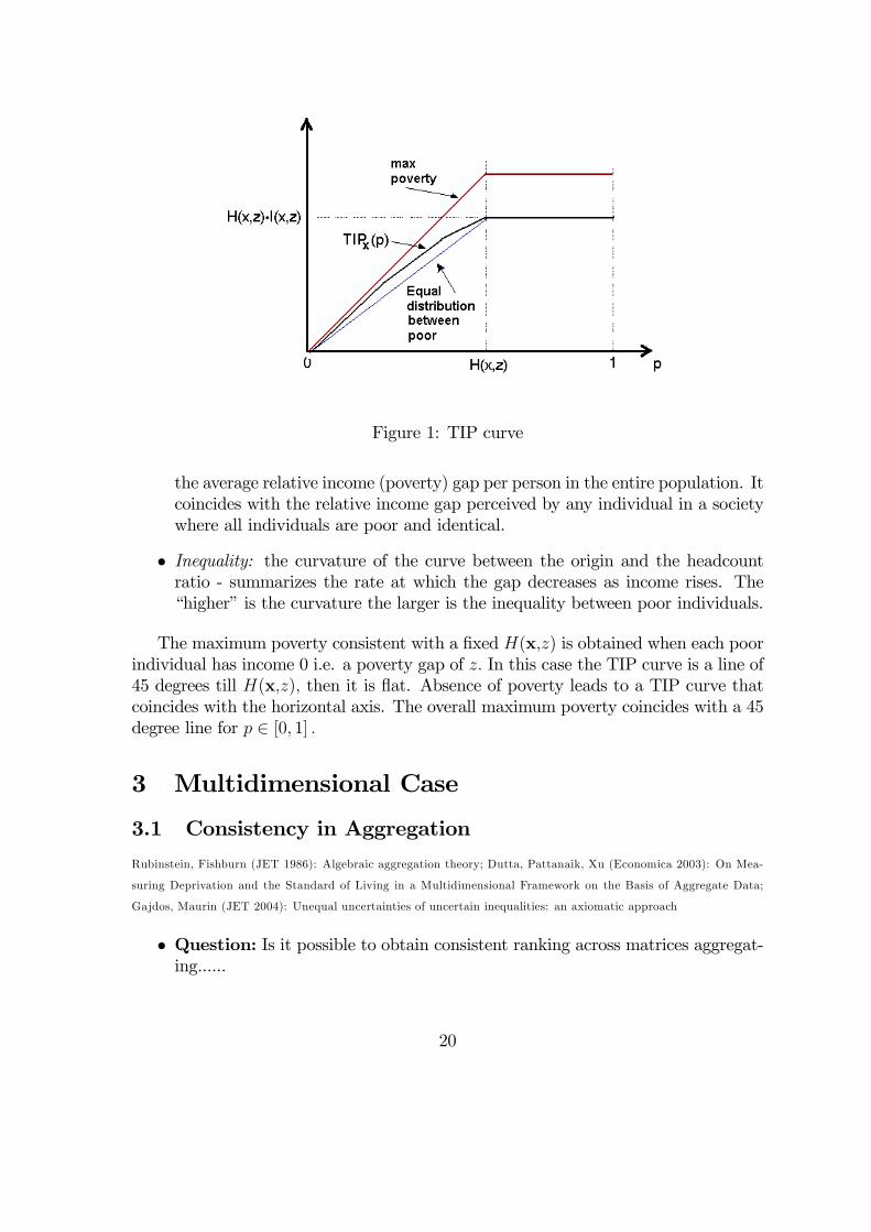
Figure 1: TIP curve
the average relative income (poverty) gap per person in the entire population. Itcoincides with the relative income gap perceived by any individual in a societywhere all individuals are poor and identical.
• Inequality: the curvature of the curve between the origin and the headcountratio - summarizes the rate at which the gap decreases as income rises. The“higher” is the curvature the larger is the inequality between poor individuals.
The maximum poverty consistent with a fixed H(x,z) is obtained when each poorindividual has income 0 i.e. a poverty gap of z. In this case the TIP curve is a line of45 degrees till H(x,z), then it is flat. Absence of poverty leads to a TIP curve thatcoincides with the horizontal axis. The overall maximum poverty coincides with a 45degree line for p ∈ [0, 1] .
3 Multidimensional Case
3.1 Consistency in Aggregation
Rubinstein, Fishburn (JET 1986): Algebraic aggregation theory; Dutta, Pattanaik, Xu (Economica 2003): On Mea-
suring Deprivation and the Standard of Living in a Multidimensional Framework on the Basis of Aggregate Data;
Gajdos, Maurin (JET 2004): Unequal uncertainties of uncertain inequalities: an axiomatic approach
• Question: Is it possible to obtain consistent ranking across matrices aggregat-ing......
20
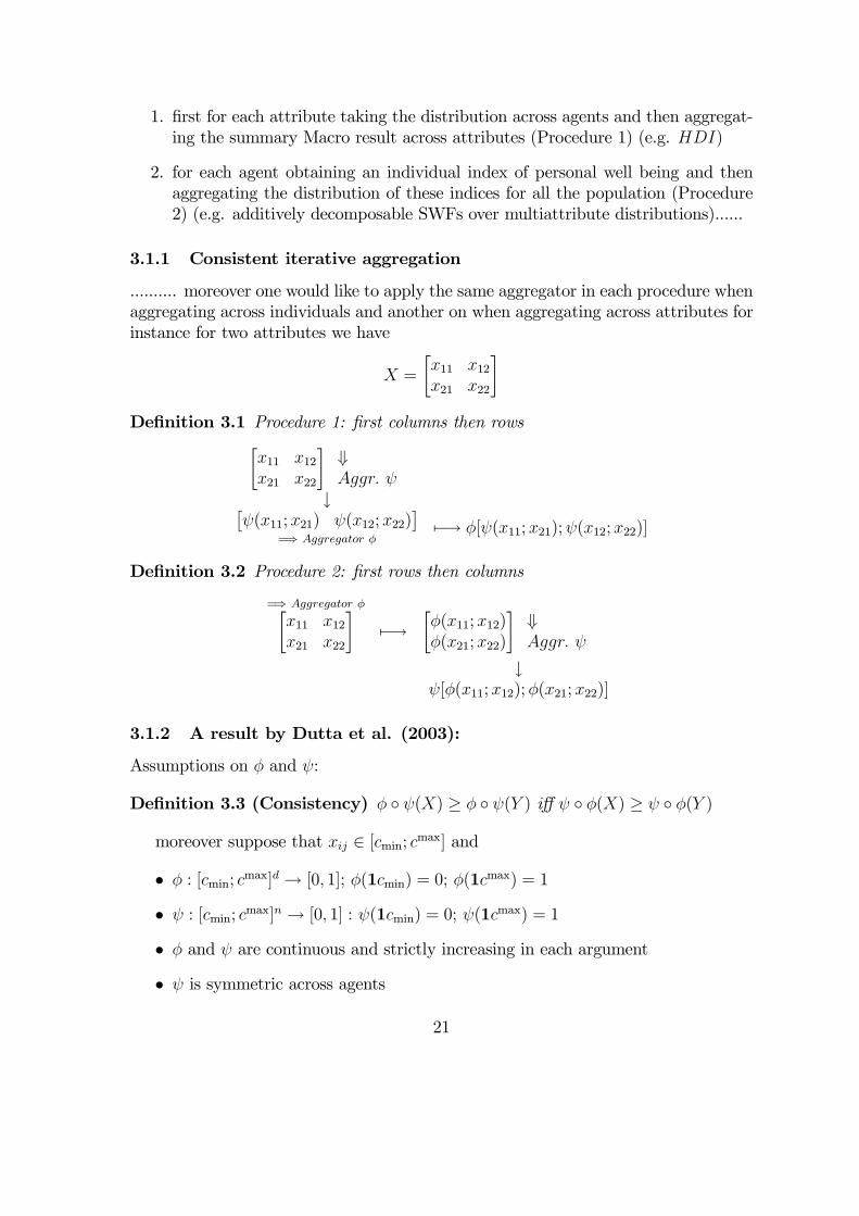
1. first for each attribute taking the distribution across agents and then aggregat-ing the summary Macro result across attributes (Procedure 1) (e.g. HDI)
2. for each agent obtaining an individual index of personal well being and thenaggregating the distribution of these indices for all the population (Procedure2) (e.g. additively decomposable SWFs over multiattribute distributions)......
3.1.1 Consistent iterative aggregation
.......... moreover one would like to apply the same aggregator in each procedure whenaggregating across individuals and another on when aggregating across attributes forinstance for two attributes we have
X =
·x11 x12x21 x22
¸Definition 3.1 Procedure 1: first columns then rows·
x11 x12x21 x22
¸ ⇓Aggr. ψ↓£
ψ(x11;x21) ψ(x12;x22)¤
=⇒ Aggregator φ7−→ φ[ψ(x11;x21);ψ(x12;x22)]
Definition 3.2 Procedure 2: first rows then columns
=⇒ Aggregator φ·x11 x12x21 x22
¸7−→
·φ(x11;x12)φ(x21;x22)
¸ ⇓Aggr. ψ
↓ψ[φ(x11;x12);φ(x21;x22)]
3.1.2 A result by Dutta et al. (2003):
Assumptions on φ and ψ:
Definition 3.3 (Consistency) φ ◦ ψ(X) ≥ φ ◦ ψ(Y ) iff ψ ◦ φ(X) ≥ ψ ◦ φ(Y )
moreover suppose that xij ∈ [cmin; cmax] and
• φ : [cmin; cmax]d → [0, 1]; φ(1cmin) = 0; φ(1c
max) = 1
• ψ : [cmin; cmax]n → [0, 1] : ψ(1cmin) = 0; ψ(1c
max) = 1
• φ and ψ are continuous and strictly increasing in each argument
• ψ is symmetric across agents
21
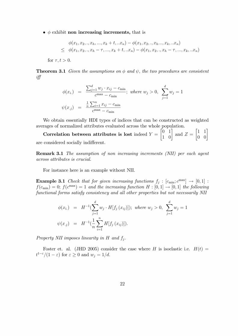
• φ exhibit non increasing increments, that is
φ(x1, x2, ., xh, ..., xk + t, ..xn)− φ(x1, x2, ., xh..., xk, ..xn)
≤ φ(x1, x2, ., xh − τ , ..., xk + t, ..xn)− φ(x1, x2, ., xh − τ , ..., xk, ..xn)
for τ , t > 0.
Theorem 3.1 Given the assumptions on φ and ψ, the two procedures are consistentiff
φ(xi.) =
Pdj=1wj · xij − cmin
cmax − cmin; where wj > 0,
dXj=1
wj = 1
ψ(x.j) =1n
Pni=1 xij − cmin
cmax − cmin
We obtain essentially HDI types of indices that can be constructed as weightedaverages of normalized attributes evaluated across the whole population.
Correlation between attributes is lost indeed Y =
·0 11 0
¸and Z =
·1 10 0
¸are considered socially indifferent.
Remark 3.1 The assumption of non increasing increments (NII) per each agentacross attributes is crucial.
For instance here is an example without NII.
Example 3.1 Check that for given increasing functions fj : [cmin; cmax] → [0, 1] :f(cmin) = 0; f(c
max) = 1 and the increasing function H : [0, 1] → [0, 1] the followingfunctional forms satisfy consistency and all other properties but not necessarily NII
φ(xi.) = H−1(dX
j=1
wj ·H[fj (xij)]); where wj > 0,dX
j=1
wj = 1
ψ(x.j) = H−1(1
n
nXi=1
H[fj (xij)]).
Property NII imposes linearity in H and fj.
Foster et. al. (JHD 2005) consider the case where H is isoelastic i.e. H(t) =t1−ε/(1− ε) for ε ≥ 0 and wj = 1/d.
22
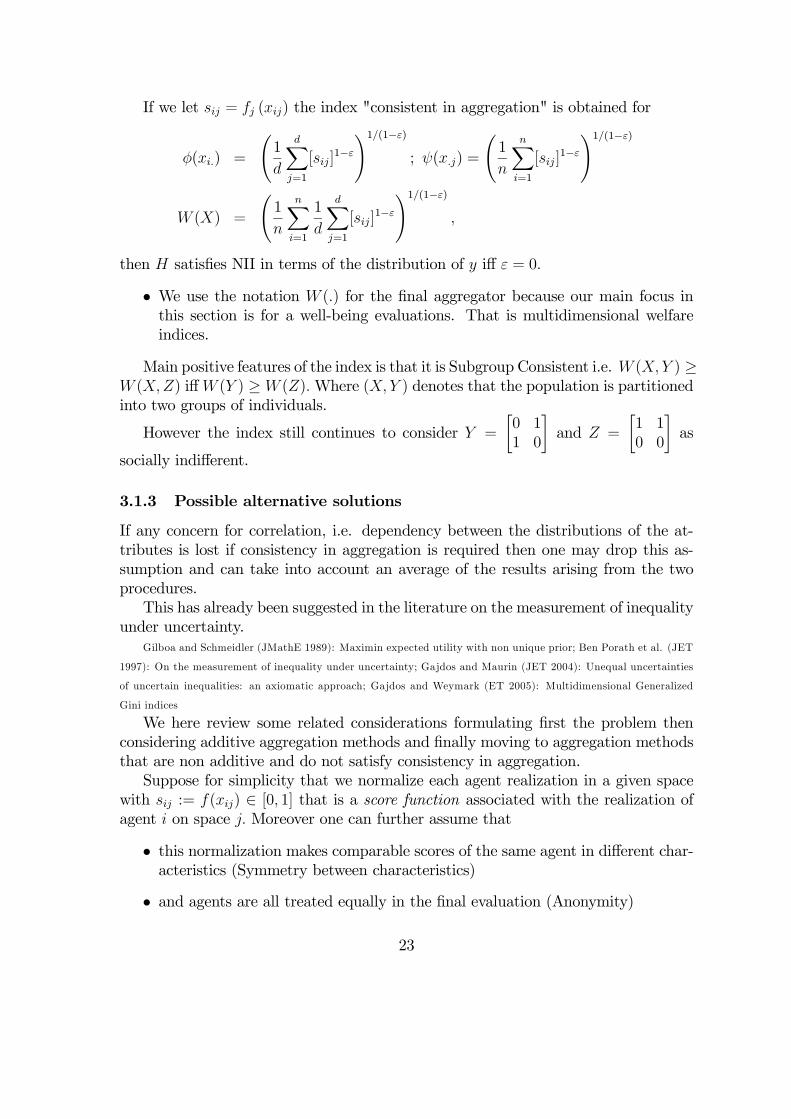
If we let sij = fj (xij) the index "consistent in aggregation" is obtained for
φ(xi.) =
Ã1
d
dXj=1
[sij]1−ε!1/(1−ε)
; ψ(x.j) =
Ã1
n
nXi=1
[sij ]1−ε!1/(1−ε)
W (X) =
Ã1
n
nXi=1
1
d
dXj=1
[sij]1−ε!1/(1−ε)
,
then H satisfies NII in terms of the distribution of y iff ε = 0.
• We use the notation W (.) for the final aggregator because our main focus inthis section is for a well-being evaluations. That is multidimensional welfareindices.
Main positive features of the index is that it is Subgroup Consistent i.e. W (X,Y ) ≥W (X,Z) iffW (Y ) ≥W (Z).Where (X,Y ) denotes that the population is partitionedinto two groups of individuals.
However the index still continues to consider Y =
·0 11 0
¸and Z =
·1 10 0
¸as
socially indifferent.
3.1.3 Possible alternative solutions
If any concern for correlation, i.e. dependency between the distributions of the at-tributes is lost if consistency in aggregation is required then one may drop this as-sumption and can take into account an average of the results arising from the twoprocedures.This has already been suggested in the literature on the measurement of inequality
under uncertainty.Gilboa and Schmeidler (JMathE 1989): Maximin expected utility with non unique prior; Ben Porath et al. (JET
1997): On the measurement of inequality under uncertainty; Gajdos and Maurin (JET 2004): Unequal uncertainties
of uncertain inequalities: an axiomatic approach; Gajdos and Weymark (ET 2005): Multidimensional Generalized
Gini indices
We here review some related considerations formulating first the problem thenconsidering additive aggregation methods and finally moving to aggregation methodsthat are non additive and do not satisfy consistency in aggregation.Suppose for simplicity that we normalize each agent realization in a given space
with sij := f(xij) ∈ [0, 1] that is a score function associated with the realization ofagent i on space j. Moreover one can further assume that
• this normalization makes comparable scores of the same agent in different char-acteristics (Symmetry between characteristics)
• and agents are all treated equally in the final evaluation (Anonymity)
23
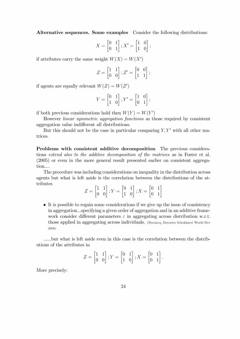
Alternative sequences. Some examples Consider the following distributions:
X =
·0 10 1
¸;X 0 =
·1 01 0
¸;
if attributes carry the same weight W (X) =W (X 0)
Z =
·1 10 0
¸;Z 0 =
·0 01 1
¸;
if agents are equally relevant W (Z) =W (Z 0)
Y =
·0 11 0
¸;Y 0 =
·1 00 1
¸;
if both previous considerations hold then W (Y ) =W (Y 0)However linear symmetric aggregation functions as those required by consistent
aggregation value indifferent all distributions.But this should not be the case in particular comparing Y, Y 0 with all other ma-
trices.
Problems with consistent additive decomposition The previous considera-tions extend also to the additive decomposition of the matrices as in Foster et al.(2005) or even in the more general result presented earlier on consistent aggrega-tion....The procedure was including considerations on inequality in the distribution across
agents but what is left aside is the correlation between the distributions of the at-tributes
Z =
·1 10 0
¸;Y =
·0 11 0
¸;X =
·0 10 1
¸• It is possible to regain some considerations if we give up the issue of consistencyin aggregation...specifying a given order of aggregation and in an additive frame-work consider different parameters ε in aggregating across distribution w.r.t.those applied in aggregating across individuals. (Decancq, Decoster Schokkaert World Dev2008)
......but what is left aside even in this case is the correlation between the distrib-utions of the attributes in
Z =
·1 10 0
¸;Y =
·0 11 0
¸;X =
·0 10 1
¸.
More precisely:
24
• Depending on the order of aggregation if we start first deriving an individualindex of well being symmetric in attributes then W (Y ) =W (X).
• If we aggregate first across attributes deriving a Macro index of the distributionacross individuals then W (Y ) =W (Z) This second result is more controversialand highlight some critical aspects underlying the procedure that first aggre-gates across attributes. For more general results in this direction see Pattanaiket al. (2008)
The general critical issue in comparing Y and Z is the increase in the correlationbetween attributes in Z.
From Y =
·0 11 0
¸to Z =
·1 10 0
¸we have transferred attribute 1 from agent 2 to
agent 1 that now clearly dominates the latter.
Definition 3.4 (CIT) In general a Correlation Increasing Transfer CIT (i, j)is a sequence of "rearrangements" of the distribution of attributes (one attribute perstep of the sequence) involving only two individuals (i, j) s.t. as the result of theprocess one individual ends up being weakly dominated by the other in any attribute.
Epstein and Tanny (CanJEc1980), Tsui (JET 1995, SCW 1999)
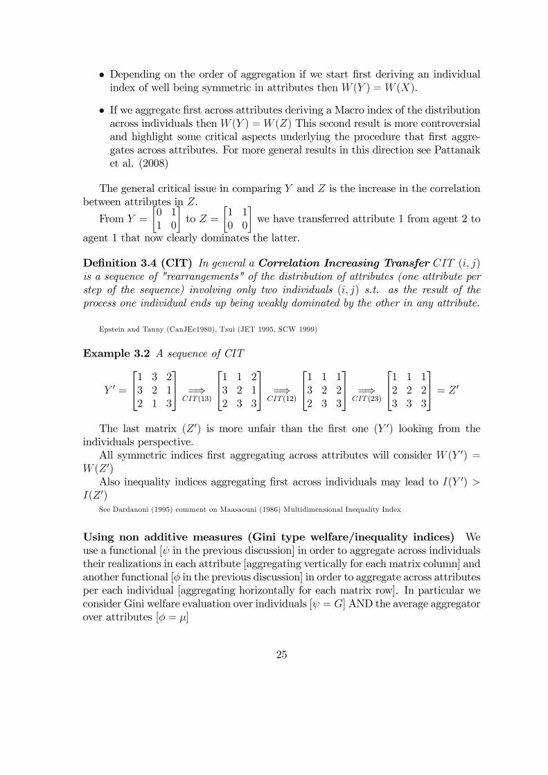
Example 3.2 A sequence of CIT
Y 0 =
1 3 23 2 12 1 3
=⇒CIT (13)
1 1 23 2 12 3 3
=⇒CIT (12)
1 1 13 2 22 3 3
=⇒CIT (23)
1 1 12 2 23 3 3
= Z 0
The last matrix (Z 0) is more unfair than the first one (Y 0) looking from theindividuals perspective.All symmetric indices first aggregating across attributes will consider W (Y 0) =
W (Z 0)Also inequality indices aggregating first across individuals may lead to I(Y 0) >
I(Z 0)See Dardanoni (1995) comment on Maasaouni (1986) Multidimensional Inequality Index
Using non additive measures (Gini type welfare/inequality indices) Weuse a functional [ψ in the previous discussion] in order to aggregate across individualstheir realizations in each attribute [aggregating vertically for each matrix column] andanother functional [φ in the previous discussion] in order to aggregate across attributesper each individual [aggregating horizontally for each matrix row]. In particular weconsider Gini welfare evaluation over individuals [ψ = G] AND the average aggregatorover attributes [φ = µ]
25
Definition 3.5 First procedure (average of Gini indices of the agents distributionfor each attribute): aggregating for each attribute taking the Gini index across agentsAND then averaging the obtained result.
Let v1 ≥ ... ≥ vi ≥ vi+1 ≥ ... ≥ vn ≥ 0 whereP
i vi = 1 let s(i)j denote theincreased order of sij for each attribute j across agents i.e. s(1)j ≤ s(2)j ≤ ... ≤ s(n)jthen
Gj(s.j) =nXi=1
vi · s(i)j
averaging across all attributes we get
G1(S) =1
d
dXj=1
nXi=1
vi · s(i)j.
Remark 3.2 Note that we assume symmetry across attributes thus the weightingfunction vi applied in Gj(s.j) is independent from j.
Second procedure with Gini type indices.
Definition 3.6 Second procedure (Gini index of average agent score): Averageover attributes for each agent AND Gini aggregation over individuals scores.
Average score of agent i :
µi = µ(si.) =1
d
dXj=1
sij;
let µ[i] denote the increased order of µi i.e. µ[1] ≤ µ[2] ≤ ... ≤ µ[n] and let β1 ≥ ... ≥βi ≥ βi+1 ≥ ... ≥ βn ≥ 0 where
Pi βi = 1 then
G2(S) =nXi=1
βi · µ[i] =nXi=1
βi ·Ã1
d
dXj=1
s[i]j
!=1
d
dXj=1
nXi=1
βi · s[i]j.
Remark 3.3 Note that the order of s(i)j and s[i]j does not necessarily coincide. Inparticular for a given attribute j the elements s(i)j are ranked in increasing order interms of values of sij, while the elements s[i]j are ranked according to the increasingorder of the elements µi. Thus s(i)j = s[i]j only if the order of the scoring functionssij for attribute j is the same as the order of the average scores µi.
• If the rank correlation of each attribute across agent is perfectly positive thens(i)j = s[i]j for any i and j, thus G1(S) = G2(S) if βi = vi.
• However note that in general G1(S) = G2(S) only if βi = vi = 1/n.
26
Remarks on Gini indices Getting back to the original matrices
X =
·0 10 1
¸;Z =
·1 10 0
¸;Y =
·0 11 0
¸;
recall that X 0, Z 0, Y 0 are obtained permuting either rows or columns thus they obtainthe same evaluation of the symmetric distributions X,Z, Y respectively. Applyingthe mentioned procedure one gets:
G1(X) = 1/2 G2(Z) = 1− β1G1(Z) = G1(Y ) = 1− v1 G2(X) = G2(Y ) = 1/2
The final index that considers a weighted average of G1(.) and G2(.) according to
W (S) := α ·G1(S) + (1− α) ·G2(S)
will give:
W (Y ) = α · (1− v1) + (1− α) · 1/2 ≤ 1/2W (X) = 1/2
W (Z) = α · (1− v1) + (1− α) · (1− β1) ≤ 1/2
recalling that (1− v1) ≤ 1/2 and (1− β1) ≤ 1/2.More precisely if α ∈ (0, 1), 1/2 < v1and 1/2 < β1 then
W (X) > W (Y ) > W (Z).
Remark 3.4 Note this mixed procedure is different from Hicks (1997 World Dev.)proposal of taking the average of the Gini welfare index of the distribution of eachattribute. (This measure coincides with the one obtained applying only the first pro-cedure)
Remark 3.5 Gajdos and Weymark (ET 2005) characterize families of Generalizedaverages across attributes of Gini indices across individuals per each attribute. (Againin line with the application of the first procedure only)
However as already pointed out for these measures
Z =
·1 10 0
¸and Y =
·0 11 0
¸are considered socially indifferent thereby neglecting considerations based on corre-lation in the distribution of the attributes.
27
What about applying a Gini type evaluation to the overall matrix? Aproblem arises due to comonotonic independence (across attributes). Consider ma-trices
H =
·1/2 00 0
¸;H 0 =
·0 01/2 0
¸;K =
·1/2 1/21/2 0
¸;
note that K is comonotonic w.r.t. H and H 0 because the ranking of the attributesis the same in all matrices: taken any pair of cells ij and i0j0 it is always true thatHij ≥ Hi0j0 ⇐⇒ Kij ≥ Ki0j0 (similarly for comparisons of K and H 0).
• Comonotonic Independence is the key property characterizing Gini type (i.e.rank dependent) evaluations!
By Comonotonic independence between K and H and K and H 0 it follows thatfor a Gini index G
G(H +K) ≥ G(H 0 +K)⇐⇒ G(H) ≥ G(H 0)
...but G(H) = G(H 0) by anonymity (i.e. symmetry across individuals), thus
G(H +K) = G(H 0 +K)
where
H +K =
·1 1/21/2 0
¸;H 0 +K =
·1/2 1/21 0
¸.
Note that the general indication for the multivariate Gini index G(H + K) =G(H 0+K) is in line with the one obtained following the first procedure of aggregationfirst across individuals and then averaging across attributes that will lead to G1(H +K) = G1(H 0+K). Once again correlation is neglected indeed H+K can be obtainedfrom H 0+K through a Correlation Increasing Transfer in the first attribute thus onewould expect that W (H +K) ≤ W (H 0 +K) as it is the case applying the previousmixed two steps procedure.
• Open question...appropriate definition of multidimensional Gini functionals...
4 Multidimensional orders
In this section we move from multidimensional indices to dominance conditions.The key component of interest in the multidimensional framework is still the
dependence between attributesDifferent tools can be applied:
• Multidimensional Majorization.• Multidimensional versions of Lorenz and Generalized Lorenz curves and relateddominance conditions.
• Multidimensional Stochastic dominance conditions based on stochastic ordersspecified in the unidimensional framework.
28
4.1 Multidimensional Majorization
Kolm (QJE 1977): Multidimensional egalitarianism; Koshevoy (SCW 1995): Multivariate Lorenz majorization; Ko-
shevoy, Mosler (JASA 1996): The Lorenz zonoid of a multivariate distribution; Koshevoy, Mosler (AStA 2007):
Multivariate Lorenz dominance based on zonoids; Marshall, A. W. and Olkin, I. (1979): Inequalities: Theory of
Majorization and Its Applications. New York: Academic Press; Weymark (2004) The normative approach to the
measurement of multidimensional inequality; Savaglio (2004) Multidimensional inequality: a survey
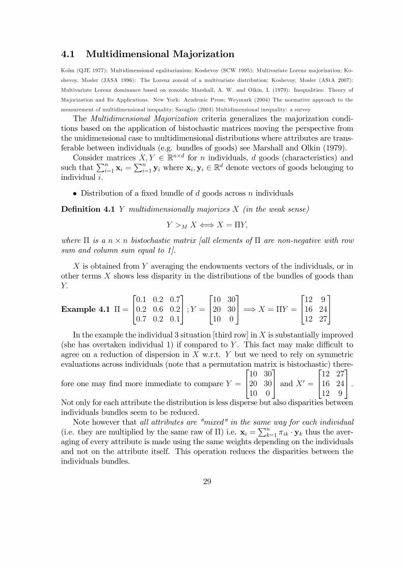
The Multidimensional Majorization criteria generalizes the majorization condi-tions based on the application of bistochastic matrices moving the perspective fromthe unidimensional case to multidimensional distributions where attributes are trans-ferable between individuals (e.g. bundles of goods) see Marshall and Olkin (1979).Consider matrices X,Y ∈ Rn×d for n individuals, d goods (characteristics) and
such thatPn
i=1 xi =Pn
i=1 yi where xi,yi ∈ Rd denote vectors of goods belonging toindividual i.
• Distribution of a fixed bundle of d goods across n individualsDefinition 4.1 Y multidimensionally majorizes X (in the weak sense)
Y >M X ⇐⇒ X = ΠY,
where Π is a n× n bistochastic matrix [all elements of Π are non-negative with rowsum and column sum equal to 1].
X is obtained from Y averaging the endowments vectors of the individuals, or inother terms X shows less disparity in the distributions of the bundles of goods thanY.
Example 4.1 Π =
0.1 0.2 0.70.2 0.6 0.20.7 0.2 0.1
;Y =10 3020 3010 0
=⇒ X = ΠY =
12 916 2412 27
In the example the individual 3 situation [third row] inX is substantially improved
(she has overtaken individual 1) if compared to Y . This fact may make difficult toagree on a reduction of dispersion in X w.r.t. Y but we need to rely on symmetricevaluations across individuals (note that a permutation matrix is bistochastic) there-
fore one may find more immediate to compare Y =
10 3020 3010 0
and X 0 =
12 2716 2412 9
.Not only for each attribute the distribution is less disperse but also disparities betweenindividuals bundles seem to be reduced.Note however that all attributes are "mixed" in the same way for each individual
(i.e. they are multiplied by the same raw of Π) i.e. xi =Pn
k=1 πik · yk thus the aver-aging of every attribute is made using the same weights depending on the individualsand not on the attribute itself. This operation reduces the disparities between theindividuals bundles.
29
A welfare interpretation Consider matrices X,Y ∈ Rn×d such thatPn
i=1 xi =Pni=1 yi
Theorem 4.1 Y >M X is equivalent to the following conditions(I) φ(Y ) ≤ φ(X) for all φ : Rn×d→ R which are S-concave;(II)
Pni=1 u(yi) ≤
Pni=1 u(xi) for all u : Rd→ R which are concave [they can also
be increasing].
S-Concave function: symmetric functions such that φ(Y ) ≤ φ(ΠY )The distribution X of a fixed amount of resources improves welfareDoes it means that we have also less inequality in terms of the distribution of the
concave and increasing utilities u(yi)?Will it be possible to decompose the change from Y to X in terms of progressive
transfers?
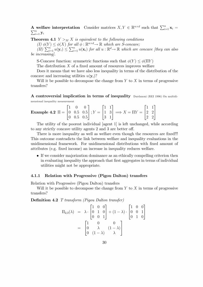
A controversial implication in terms of inequality Dardanoni (REI 1996) On multidi-
mensional inequality measurement
Example 4.2 Π =
1 0 00 0.5 0.50 0.5 0.5
;Y =1 11 33 1
=⇒ X = ΠY =
1 12 22 2
The utility of the poorest individual [agent 1] is left unchanged, while according
to any strictly concave utility agents 2 and 3 are better off.There is more inequality as well as welfare even though the resources are fixed!!!
This outcome contradicts the link between welfare and inequality evaluations in theunidimensional framework. For unidimensional distributions with fixed amount ofattributes (e.g. fixed income) an increase in inequality reduces welfare.
• If we consider majorization dominance as an ethically compelling criterion thenin evaluating inequality the approach that first aggregates in terms of individualutilities might not be appropriate.
4.1.1 Relation with Progressive (Pigou Dalton) transfers
Relation with Progressive (Pigou Dalton) transfersWill it be possible to decompose the change from Y to X in terms of progressive
transfers?
Definition 4.2 T transform (Pigou Dalton transfer)
Π2,3(λ) = λ ·1 0 00 1 00 0 1
+ (1− λ) ·1 0 00 0 10 1 0
=
1 0 00 λ (1− λ)0 (1− λ) λ
30
a convex combination of identity matrix and a permutation matrix involving a per-mutation of 2 individuals.
These transformations are those underlying the Pigou Dalton progressive transferin the unidimensional case.Will it be possible to decompose the change from Y to X in terms of progressive
transfers?
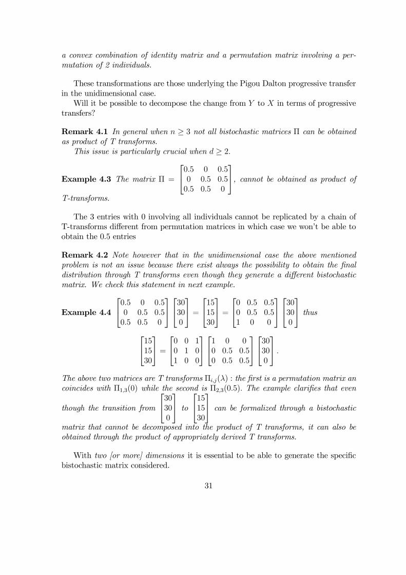
Remark 4.1 In general when n ≥ 3 not all bistochastic matrices Π can be obtainedas product of T transforms.This issue is particularly crucial when d ≥ 2.
Example 4.3 The matrix Π =
0.5 0 0.50 0.5 0.50.5 0.5 0
, cannot be obtained as product ofT-transforms.
The 3 entries with 0 involving all individuals cannot be replicated by a chain ofT-transforms different from permutation matrices in which case we won’t be able toobtain the 0.5 entries
Remark 4.2 Note however that in the unidimensional case the above mentionedproblem is not an issue because there exist always the possibility to obtain the finaldistribution through T transforms even though they generate a different bistochasticmatrix. We check this statement in next example.
Example 4.4
0.5 0 0.50 0.5 0.50.5 0.5 0
30300
=151530
=0 0.5 0.50 0.5 0.51 0 0
30300
thus151530
=0 0 10 1 01 0 0
1 0 00 0.5 0.50 0.5 0.5
30300
.The above two matrices are T transforms Πi,j(λ) : the first is a permutation matrix ancoincides with Π1,3(0) while the second is Π2,3(0.5). The example clarifies that even
though the transition from
30300
to151530
can be formalized through a bistochasticmatrix that cannot be decomposed into the product of T transforms, it can also beobtained through the product of appropriately derived T transforms.
With two [or more] dimensions it is essential to be able to generate the specificbistochastic matrix considered.
31
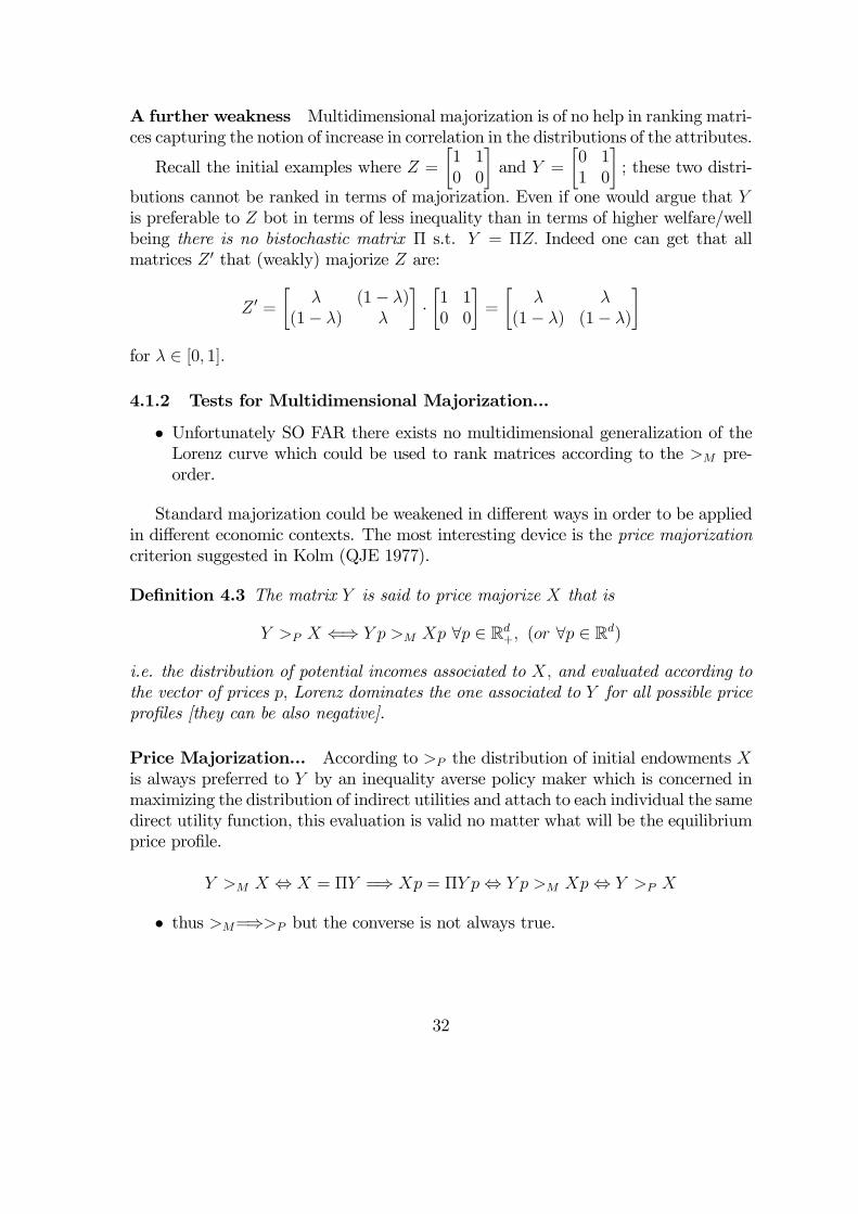
A further weakness Multidimensional majorization is of no help in ranking matri-ces capturing the notion of increase in correlation in the distributions of the attributes.
Recall the initial examples where Z =·1 10 0
¸and Y =
·0 11 0
¸; these two distri-
butions cannot be ranked in terms of majorization. Even if one would argue that Yis preferable to Z bot in terms of less inequality than in terms of higher welfare/wellbeing there is no bistochastic matrix Π s.t. Y = ΠZ. Indeed one can get that allmatrices Z 0 that (weakly) majorize Z are:
Z 0 =·
λ (1− λ)(1− λ) λ
¸··1 10 0
¸=
·λ λ
(1− λ) (1− λ)
¸for λ ∈ [0, 1].
4.1.2 Tests for Multidimensional Majorization...
• Unfortunately SO FAR there exists no multidimensional generalization of theLorenz curve which could be used to rank matrices according to the >M pre-order.
Standard majorization could be weakened in different ways in order to be appliedin different economic contexts. The most interesting device is the price majorizationcriterion suggested in Kolm (QJE 1977).
Definition 4.3 The matrix Y is said to price majorize X that is
Y >P X ⇐⇒ Y p >M Xp ∀p ∈ Rd+, (or ∀p ∈ Rd)
i.e. the distribution of potential incomes associated to X, and evaluated according tothe vector of prices p, Lorenz dominates the one associated to Y for all possible priceprofiles [they can be also negative].
Price Majorization... According to >P the distribution of initial endowments Xis always preferred to Y by an inequality averse policy maker which is concerned inmaximizing the distribution of indirect utilities and attach to each individual the samedirect utility function, this evaluation is valid no matter what will be the equilibriumprice profile.
Y >M X ⇔ X = ΠY =⇒ Xp = ΠY p⇔ Y p >M Xp⇔ Y >P X
• thus >M=⇒>P but the converse is not always true.
32
There exist multidimensional generalizations of the Lorenz curve that can be usedto test >Pboth when p ∈ Rd
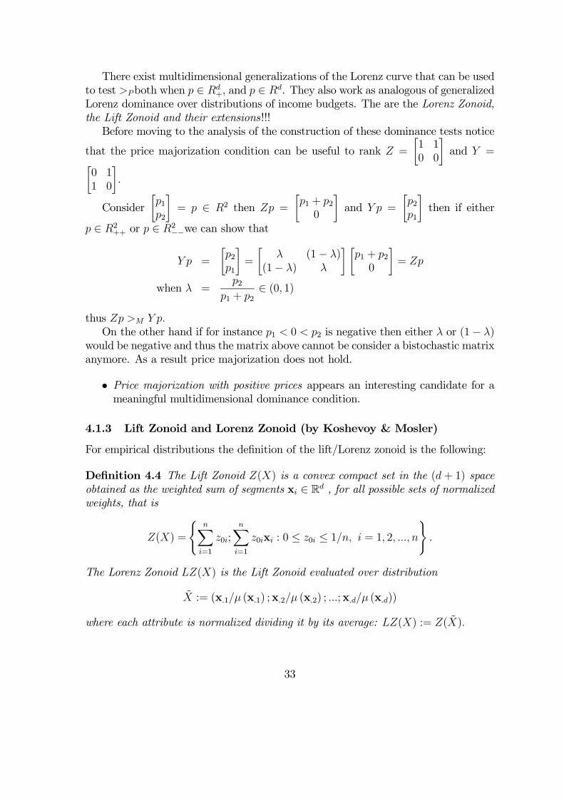
+, and p ∈ Rd. They also work as analogous of generalizedLorenz dominance over distributions of income budgets. The are the Lorenz Zonoid,the Lift Zonoid and their extensions!!!Before moving to the analysis of the construction of these dominance tests notice
that the price majorization condition can be useful to rank Z =
·1 10 0
¸and Y =·
0 11 0
¸.
Consider·p1p2
¸= p ∈ R2 then Zp =
·p1 + p20
¸and Y p =
·p2p1
¸then if either
p ∈ R2++ or p ∈ R2−−we can show that
Y p =
·p2p1
¸=
·λ (1− λ)
(1− λ) λ
¸ ·p1 + p20
¸= Zp
when λ =p2
p1 + p2∈ (0, 1)
thus Zp >M Y p.On the other hand if for instance p1 < 0 < p2 is negative then either λ or (1− λ)
would be negative and thus the matrix above cannot be consider a bistochastic matrixanymore. As a result price majorization does not hold.
• Price majorization with positive prices appears an interesting candidate for ameaningful multidimensional dominance condition.
4.1.3 Lift Zonoid and Lorenz Zonoid (by Koshevoy & Mosler)
For empirical distributions the definition of the lift/Lorenz zonoid is the following:
Definition 4.4 The Lift Zonoid Z(X) is a convex compact set in the (d + 1) spaceobtained as the weighted sum of segments xi ∈ Rd , for all possible sets of normalizedweights, that is
Z(X) =
(nXi=1
z0i;nXi=1
z0ixi : 0 ≤ z0i ≤ 1/n, i = 1, 2, ..., n).
The Lorenz Zonoid LZ(X) is the Lift Zonoid evaluated over distribution
X := (x.1/µ (x.1) ;x.2/µ (x.2) ; ...;x.d/µ (x.d))
where each attribute is normalized dividing it by its average: LZ(X) := Z(X).
33
Zonoids: the intuition
• Take all subsets of the population of a given relative size z0 ∈ [0, 1] (e.g. 50%)[where z0 = Σiz0i] what is the aggregate (divided by n) realization in the ddimensional space of the resources of any of these subsets covering a z0 pro-portion of population? Take the convex hull of all these distributions in the ddimensional space. We have obtained the section of the Lift Zonoid for afixed value of population share z0. As z0 moves from 0 to 1 we constructthe Lift Zonoid. For finite populations it is necessary to "convexify" all sectionscorresponding to adjacent proportions of population.
• In order to get the Lorenz Zonoid we need just to apply the same logic tothe normalized distributions of each attribute. So normalize each columns inrelative terms so that any aggregate amount sums to n.
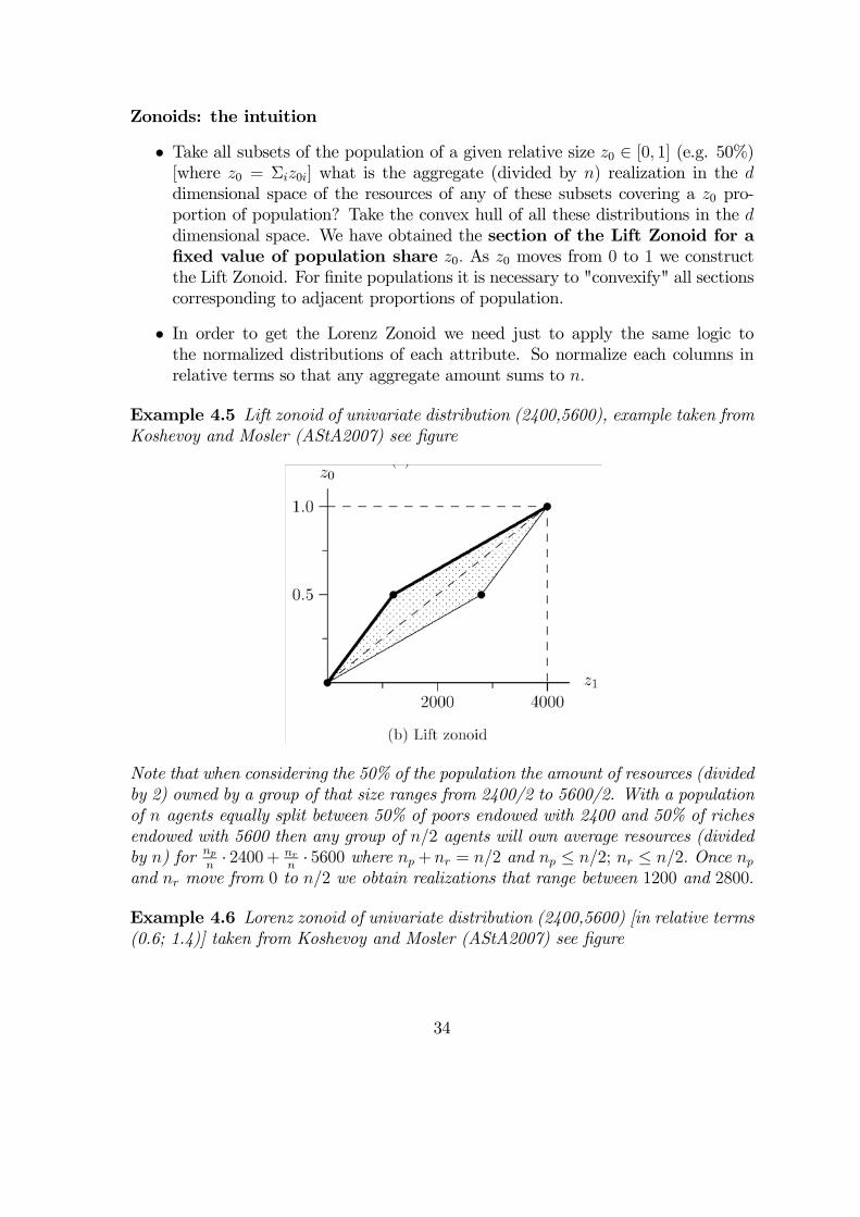
Example 4.5 Lift zonoid of univariate distribution (2400,5600), example taken fromKoshevoy and Mosler (AStA2007) see figure
Note that when considering the 50% of the population the amount of resources (dividedby 2) owned by a group of that size ranges from 2400/2 to 5600/2. With a populationof n agents equally split between 50% of poors endowed with 2400 and 50% of richesendowed with 5600 then any group of n/2 agents will own average resources (dividedby n) for np
n· 2400+ nr
n· 5600 where np+nr = n/2 and np ≤ n/2; nr ≤ n/2. Once np
and nr move from 0 to n/2 we obtain realizations that range between 1200 and 2800.
Example 4.6 Lorenz zonoid of univariate distribution (2400,5600) [in relative terms(0.6; 1.4)] taken from Koshevoy and Mosler (AStA2007) see figure
34
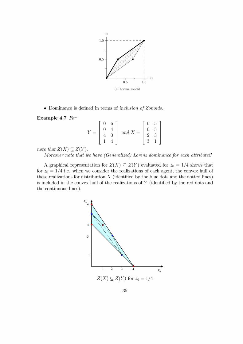
• Dominance is defined in terms of inclusion of Zonoids.Example 4.7 For
Y =
0 60 44 01 4
and X =
0 50 52 33 1
note that Z(X) ⊆ Z(Y ).Moreover note that we have (Generalized) Lorenz dominance for each attribute!!
A graphical representation for Z(X) ⊆ Z(Y ) evaluated for z0 = 1/4 shows thatfor z0 = 1/4 i.e. when we consider the realizations of each agent, the convex hull ofthese realizations for distribution X (identified by the blue dots and the dotted lines)is included in the convex hull of the realizations of Y (identified by the red dots andthe continuous lines).
4
4
6
32
1
1
3
x.1
x.2
Z(X) ⊆ Z(Y ) for z0 = 1/4
35
Clearly inclusion of the convex hull of the average realization of groups of a given sizeshould also be checked for z0 = 2/4, and z0 = 3/4 (for z0 = 1 the zonoids coincidegiven that the aggregate total amount of resources is the same in X and Y ). Furthercalculations will show that these conditions hold thus Z(X) ⊆ Z(Y ).
Remark 4.3 There is no (4× 4) bistochastic matrix Π such that X = ΠY for Xand Y presented in the previous example.In order to accommodate for the transformation from Y to X involving the first
two individuals the only admissible matrix should be
Π =
0.5 0.5 0 00.5 0.5 0 00 0 a b0 0 c d
.If we set a = 1/3; b = 2/3 in order to accommodate for the first attribute of the thirdindividual we cannot obtain the distribution in X of her second attribute!!!
This remark clarifies that
Z(X) ⊆ Z(Y ) 6=⇒ Y >M X.
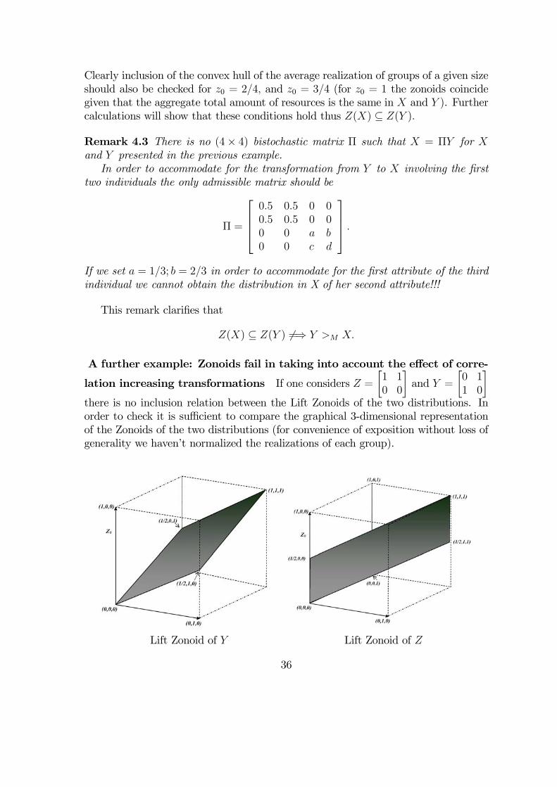
A further example: Zonoids fail in taking into account the effect of corre-
lation increasing transformations If one considers Z =·1 10 0
¸and Y =
·0 11 0
¸there is no inclusion relation between the Lift Zonoids of the two distributions. Inorder to check it is sufficient to compare the graphical 3-dimensional representationof the Zonoids of the two distributions (for convenience of exposition without loss ofgenerality we haven’t normalized the realizations of each group).
Lift Zonoid of Y Lift Zonoid of Z
36
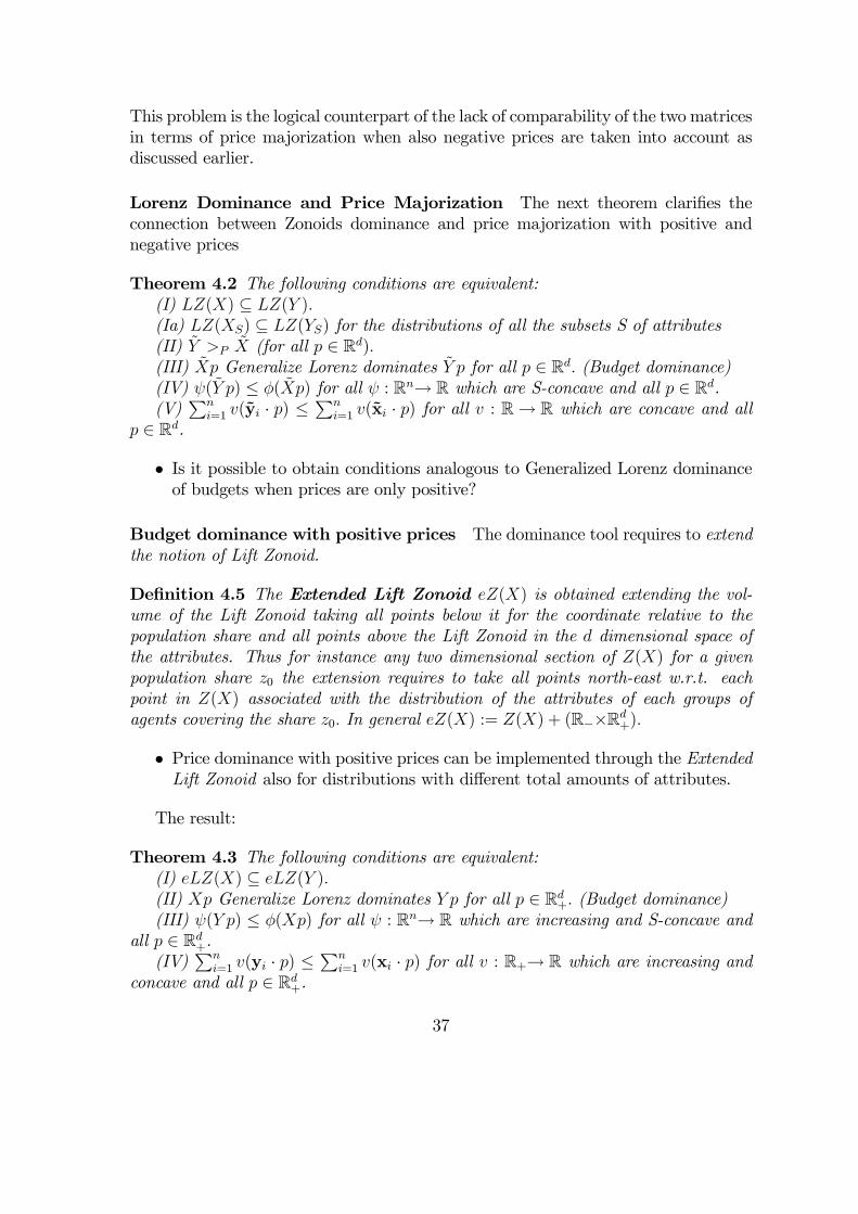
This problem is the logical counterpart of the lack of comparability of the two matricesin terms of price majorization when also negative prices are taken into account asdiscussed earlier.
Lorenz Dominance and Price Majorization The next theorem clarifies theconnection between Zonoids dominance and price majorization with positive andnegative prices
Theorem 4.2 The following conditions are equivalent:(I) LZ(X) ⊆ LZ(Y ).(Ia) LZ(XS) ⊆ LZ(YS) for the distributions of all the subsets S of attributes(II) Y >P X (for all p ∈ Rd).(III) Xp Generalize Lorenz dominates Y p for all p ∈ Rd. (Budget dominance)(IV) ψ(Y p) ≤ φ(Xp) for all ψ : Rn→ R which are S-concave and all p ∈ Rd.(V)
Pni=1 v(yi · p) ≤
Pni=1 v(xi · p) for all v : R→ R which are concave and all
p ∈ Rd.
• Is it possible to obtain conditions analogous to Generalized Lorenz dominanceof budgets when prices are only positive?
Budget dominance with positive prices The dominance tool requires to extendthe notion of Lift Zonoid.
Definition 4.5 The Extended Lift Zonoid eZ(X) is obtained extending the vol-ume of the Lift Zonoid taking all points below it for the coordinate relative to thepopulation share and all points above the Lift Zonoid in the d dimensional space ofthe attributes. Thus for instance any two dimensional section of Z(X) for a givenpopulation share z0 the extension requires to take all points north-east w.r.t. eachpoint in Z(X) associated with the distribution of the attributes of each groups ofagents covering the share z0. In general eZ(X) := Z(X) + (R−×Rd
+).
• Price dominance with positive prices can be implemented through the ExtendedLift Zonoid also for distributions with different total amounts of attributes.
The result:
Theorem 4.3 The following conditions are equivalent:(I) eLZ(X) ⊆ eLZ(Y ).(II) Xp Generalize Lorenz dominates Y p for all p ∈ Rd
+. (Budget dominance)(III) ψ(Y p) ≤ φ(Xp) for all ψ : Rn→ R which are increasing and S-concave and
all p ∈ Rd+.
(IV)Pn
i=1 v(yi · p) ≤Pn
i=1 v(xi · p) for all v : R+→ R which are increasing andconcave and all p ∈ Rd
+.
37
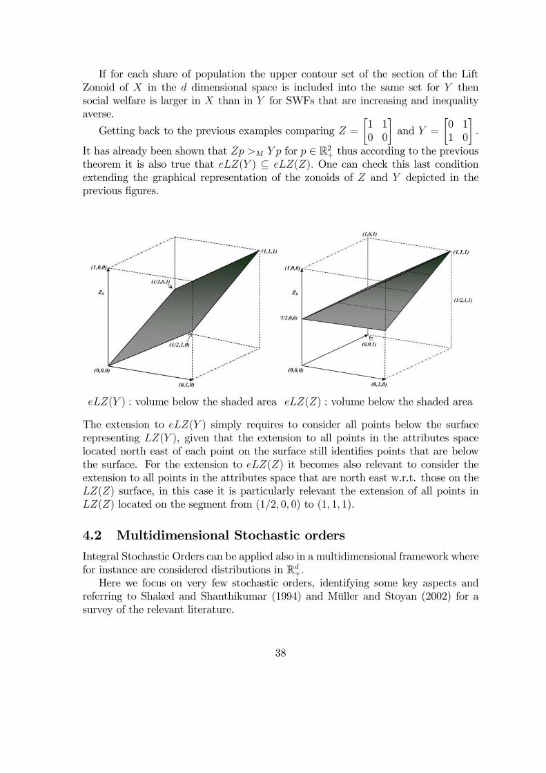
If for each share of population the upper contour set of the section of the LiftZonoid of X in the d dimensional space is included into the same set for Y thensocial welfare is larger in X than in Y for SWFs that are increasing and inequalityaverse.
Getting back to the previous examples comparing Z =·1 10 0
¸and Y =
·0 11 0
¸.
It has already been shown that Zp >M Y p for p ∈ R2+ thus according to the previoustheorem it is also true that eLZ(Y ) ⊆ eLZ(Z). One can check this last conditionextending the graphical representation of the zonoids of Z and Y depicted in theprevious figures.
eLZ(Y ) : volume below the shaded area eLZ(Z) : volume below the shaded area
The extension to eLZ(Y ) simply requires to consider all points below the surfacerepresenting LZ(Y ), given that the extension to all points in the attributes spacelocated north east of each point on the surface still identifies points that are belowthe surface. For the extension to eLZ(Z) it becomes also relevant to consider theextension to all points in the attributes space that are north east w.r.t. those on theLZ(Z) surface, in this case it is particularly relevant the extension of all points inLZ(Z) located on the segment from (1/2, 0, 0) to (1, 1, 1).
4.2 Multidimensional Stochastic orders
Integral Stochastic Orders can be applied also in a multidimensional framework wherefor instance are considered distributions in Rd
+.Here we focus on very few stochastic orders, identifying some key aspects and
referring to Shaked and Shanthikumar (1994) and Müller and Stoyan (2002) for asurvey of the relevant literature.
38
Let X = (X.j : j = 1, 2, ..., d) denote the marginal distributions of each attributej with generic realization x = (x1, x2, ..., xd) identifying a d dimensional vector ofrealizations one for each attribute with
• Cumulative Distribution Function:FX(x) := P (X ≤ x) := P (X.j ≤ xj for all j = 1, 2, 3, ..., d)
with marginals FX.j(x) for j = 1, 2, 3, ..., d.
• Survival Function:FX(x) := P (X > x) := P (X.j > xj for all j = 1, 2, 3, ..., d)
• In this framework probabilities logically correspond to proportions of popula-tions in the multidimensional distribution setup.
A first result
• Let u : Rd+ → R denote an "utility" [evaluation] function over d dimensional
attributes realizations x and
dU1 := {u : u non-decreasing}i.e. if x ≥ x0 then u(x) ≥ u(x0). Thus >dU1 denotes the following integralstochastic order
Definition 4.6 The multidimensional (d-dimensions) integral stochastic order forfunctionals in dU1 requires that
X >dU1 Y ⇐⇒ZRd+
udFX ≥ZRd+
udFY ∀u ∈ dU1
Definition 4.7 (Upper Set) The set U ∈ Rd+ is an upper set iff for all x ∈ Rd
+ ifx ∈ U then y ∈ U if y ≥ x.Theorem 4.4 The following statements are equivalent:(i) X >dU1 Y(ii) P (X ∈ U) ≥ P (Y ∈ U) for all upper set U in Rd
+.
An analogous result can be obtained when focussing on comparisons of budgetswhere attributes are evaluated in terms of non negative "prices".
Definition 4.8 Let P := {p ∈ Rd+ : p1 + p2 + ...+ pd = 1}
X >1P Y ⇐⇒ZRd+
g(Xp)dFX ≥ZRd+
g(Y p)dFY ∀g ∈ 1U1 ∀p ∈ P.
39
The following statements are equivalent (Muliere and Scarsini, 1989):
Theorem 4.5 (i) X >1P Y(ii) P (Xp > t) ≥ P ((Y p > t) for all t > 0. (Dominance for all upper sets whose
boundary is an hyperplane)
Problem 4.1 Is it possible to add to the list of equivalent conditions also those oncomparisons of FX and FY or of FX and FY?
Definition 4.9 (Upper Orthant order) X <uo Y ⇐⇒ FX(t) ≥ FY(t) for allt ∈ Rd
+.
Definition 4.10 (Lower Orthant order) X <lo Y ⇐⇒ FX(t) ≤ FY(t) for allt ∈ Rd
+.
• X <uo Y and X <lo Y are independent.
• X >dU1 Y =⇒ [X <uo Y and X <lo Y ]
• [X <uo Y and X <lo Y ] 6=⇒ X >dU1 Y.
• [X <uo Y and X <lo Y ] give the Concordance order X <c Y , i.e. an order ofassociation between variables
Solution 4.1 From last set of remarks is clear that the answer to the question posedin the formation of the previous problem is NO!
Note that by construction Upper Sets are unions of Upper Orthants, but as pre-viously stated dominance for all Upper Orthants is not sufficient to guarantee domi-nance for all Upper Sets.
Definition 4.11 (∆−monotone functions) Consider the function u : Rd+ → R,
let ε > 0, 1 := (1, 1, 1, 1, ..., 1) and 1i := (0, 0, 0, 1i, 0, ..., 0)
∆εiu (x) := u (x+ ε1i)− u (x) .
Function u is ∆−monotone if for every set {i1, i2, .., ik} ⊂ {1, 2, 3, ..., d} and everyεi > 0 for i ∈ {1, 2, 3, .., k} then
∆ε1i1∆ε2
i2...∆εk
iku (x) ≥ 0.
Definition 4.12 d∆M is the set of all bounded ∆−monotone functions u : Rd+ → R.
Definition 4.13 d∆A is the set of all bounded ∆ − antitone functions u : Rd+ → R
i.e. u(x) ∈ d∆A ⇔ −u(−x) ∈ d∆M.
40
Remark 4.4 Note: ∆− antitone functions satisfy decreasing increments.
Theorem 4.6 (i) X <uo Y ⇐⇒ X >d∆M Y(ii) X <lo Y ⇐⇒ X >d∆A Y .
Definition 4.14 (Supermodular functions) The function u : Rd+ → R, is super-
modular if for all x,y ∈ Rd+
u (max{x1, y1}; ..;max{xd, yd}) + u (min{x1, y1}; ..; min{xd, yd})≥ u (x) + u (y) .
alternatively if u is twice differentiable ∂2u∂xi∂xj
≥ 0 for all i, j ∈ {1, 2, 3, .., d}, i 6= j.
Remark 4.5 A function u : Rd+ → R is supermodular if and only if
RRd+
udFX ≥RRd+
udFY whenever X is obtained from Y through a Correlation Increasing Transfor-
mation. (It is an indicator of dependence across attributes)
Definition 4.15 The set of supermodular functions is dUSM .
Consider the bivariate case:
Theorem 4.7 Let d = 2, the following statements are equivalent:(i) X >2USM∩ 2U1 Y,(ii) X <uo Y and X.j <1 Y.j for j = 1, 2
Theorem 4.8 Let d = 2, the following statements are equivalent:(i) X >2USM Y(ii) Y <lo X and X.j = Y.j for j = 1, 2(iii) X <uo Y and X.j = Y.j for j = 1, 2
Related results can be found in Atkinson and Bourguignon (1987), Bourguignonand Chakravarty (2002), Athey (2000, 2002).For d > 2 some of the equivalences may break.
Theorem 4.9 Let d = 2, and X.j = Y.j for j = 1, 2 the following statements areequivalent:(i) X >2USM Y ;(ii) Y <lo X(iii) X <uo Y(iv) Cov[f1(X.1), f2(X.2)] ≥ Cov[f1(Y.1), f2(Y.2)] for increasing functions f1, f2;(v) X >d∆M Y.
One more result by Scarsini (J appl. Prob 1998), it relates to comparisons ofmultidimensional distributions (not necessarily bivariate) with common marginals.
Theorem 4.10 If X.j = Y.j for all j = 1, 2, .., d then Y >dUSM X implies that XpLorenz dominates Y p for all p ∈ Rd
+.
With common marginals stochastic dominance in terms of supermodular functionsimplies price dominance (with positive prices).
41
A closer look at dependence between variables. The dependence structure ofa distribution can be represented by a Copula (a random vector uniformly distributedbetween [0, 1])Consider for the Frechet class Γ(FX.1, FX.2 , ...., FX.d) of d dimensional distributions
with FX.1 , FX.2 , ...., FX.d as marginals.Given a FX ∈ Γ(FX.1 , ..., FX.d) there exist a copula C : [0, 1]d → [0, 1] s.t. for all
x ∈ Rd
FX(x) = C[FX.1(x1), FX.2(x2), ..., FX.d(xd)]
and can be constructed if FX is continuous as:
C[u] := FX [F−1x.1(u1);F
−1x.2(u2); ..., F
−1x.d(ud)] u ∈ [0, 1]d.
This result clarifies a connection between comparisons of marginals when the associ-ation between the variable represented by the copula is fixed.
Theorem 4.11 If X and Y have a common copula then X.j <1 Y.j for all j =1, 2, ..., d implies X >dU1 Y .
Thus with common copula (association) then dominance in terms of the distrib-utions of each attribute is sufficient to guarantee multivariate dominance!
5 Suggested Readings
Surveys on Stochastic Orders: Shaked, M. and Shanthikumar, J. G. (1994); Müller,A. and Stoyan, D. (2002).References for Inequality, Welfare and Poverty measurement:Books: Sen (1997); Lambert, (2001); Chakravarty, (1990);Surveys: Mosler and Muliere (1998); Zheng (1997, 2000); Cowell, F. A. (2000)
Chakravarty and Muliere, (2003, 2004);
References
[1] Aaberge, R. (2004): Ranking intersecting Lorenz curves. CEIS Working Paper45.
[2] Athey, S. (2000): Characterizing properties of stochastic objective functions.Mimeo MIT.
[3] Athey, S. (2002): Monotone comparative statics under uncertainty. QuarterlyJournal of Economics, 187-223.
[4] Atkinson, A. B. (1970): On the measurement of inequality. Journal of EconomicTheory, 2, 244-263.
42
[5] Atkinson, A. B. (1987): On the measurement of poverty. Econometrica 55, 749-764.
[6] Atkinson, A.B. (2003): Multidimensional deprivation: constrasting social welfareand counting approaches. Journal of Economic Inequality, vol. 1, pp. 51—65.
[7] Atkinson, A. B. and Bourguignon, F. (1982): The comparison of multidimen-sioned distribution of economic status. Review of Economic Studies, 49, 183-201.
[8] Ben Porath, E. and Gilboa, I. (1994): Linear measures, the Gini index, and theincome-equality trade-off. Journal of Economic Theory, 18, 59-80.
[9] Ben-Porath, E., Gilboa, I., Schmeidler, D., 1997. On the measurement of in-equality under uncertainty. Journal of Economic Theory 75, 194—204.
[10] Bourguignon, F. and S. R. Chakravarty (2003): The Measurement of Multidi-mensional Poverty, Journal of Economic Inequality, 1, 25—49.
[11] Bourguignon, F. and Chakravarty, S. R. (2002): Multidimensional poverty or-derings. Delta, Working Paper 2002-22.
[12] Chakravarty, S. R. (1990): Ethical Social Index Numbers. Berlin: Springer-Verlag.
[13] Chakravarty, S. R. (2003): A generalization of the human development index.Review of Development Economics, 7, 99-114.
[14] Chakravarty, S and Muliere, P. (2003): Welfare indicators: a review and newperspectives. 1. Measurement of inequality. Metron, International Journal ofStatistics, 61, 457-497.
[15] Chakravarty, S and Muliere, P. (2004): Welfare indicators: a review and newperspectives. 2. Measurement of poverty. Metron, International Journal of Sta-tistics, 62, 247-281.
[16] Chakravarty. S. and F. Bourguignon (2008): Multidimensional Poverty Order-ings: Theory and Applications, Forthcoming in Welfare, Development, Philos-ophy and Social Science: Essays for Amartya Sen’s 75th Birthday (Volume 2:Development Economics and Policy), K. Basu and R. Kanbur (eds.), London:Oxford University Press.
[17] Chakravarty, S. R., D’Ambrosio C. (2006) The measurement of social exclusion.Review of Income and Wealth, 52 (3) , 377—398.
[18] Chateauneuf, A., Gajdos, T. and Wilthien, P. H. (2002): The principle of strongdiminishing transfer. Journal of Economic Theory, 103, 311-333.
43
[19] Cowell, F. A. (2000): Measurement of Inequality. In Handbook of Distribution(Atkinson, A. B. and Bourguignon, F. eds.) North Holland
[20] Dardanoni, V. and Lambert, P. J. (1988): Welfare rankings of income distribu-tions: a role for the variance and some insights for tax reform. Social Choice andWelfare, 5, 1-17.
[21] Dardanoni, V. (1996): OnMultidimensional Inequality Measurement inResearchon Economic Inequality: Income Distribution, Social Welfare, Inequality andPoverty (Vol. 6), eds. C. Dagum and A. Lemmi, JAI Press Inc., pp. 201-205.
[22] Dasgupta, P., Sen, A. K. and Starrett, D. (1973): Notes on the measurement ofinequality. Journal of Economic Theory, 6, 180-187.
[23] Decancq, K., Decoster, A. & Schokkaert, E. (2007). The evolution in worldinequality in well-being. Discussion Paper Series 07/04, Center for EconomicStudies, Katholieke Universiteit Leuven.
[24] Deutsch, J. and Silber J. (2005): Measuring multidimensional poverty: an em-pirical comparison of various approaches, Review of Income and Wealth 51 (1) ,145—174.
[25] Donaldson, D. and Weymark, J. A. (1980): A single-parameter generalization ofthe Gini indices of inequality. Journal of Economic Theory, 22, 67-86.
[26] Donaldson, D. and Weymark, J. A. (1983): Ethically flexible Gini indices forincome distributions in the continuum. Journal of Economic Theory, 29, 353-358.
[27] Duclos, P. Y., Sahn, D. and Younger, S. D. (2006). Robust multidimensionalpoverty comparisons. Economic Journal, 116, 943—68.
[28] Dutta I., Pattanaik P. K. and Xu Y. (2003): On Measuring Deprivation and theStandard of Living in a Multidimensional Framework on the Basis of AggregateData, Economica, 70, 197-221.
[29] Ebert, U. (1988): Measurement of inequality: an attempt at unification andgeneralization. Social Choice and Welfare, 5, 147-69.
[30] Epstein L. G. and S. M. Tanny (1980): Increasing Generalized Correlation: ADefinition and Some Economic Consequences. The Canadian Journal of Eco-nomics, 13, 16-34.
[31] Fields, G. S. and Fei, C. H. (1978): On inequality comparisons. Econometrica,46, 303-316.
44
[32] Fishburn, P. C. (1976): Continua of stochastic dominance relations for boundedprobability distributions. Journal of Mathematical Economics, 3, 295-311.
[33] Fishburn, P. C. and Willig, R. D. (1984): Transfer principles in income redistri-bution. Journal of Public Economics, 25, 323-328.
[34] Foster, J. (1985): Inequality measurement. In Fair Allocation (Young, H. P.ed.); Proceeding of Symposia in Applied Mathematics 33, 31-68. Providence:The American Mathematical Society.
[35] Foster, J.; Greer, J. and Thorbecke, D. (1984): A class of decomposable povertymeasures. Econometrica, 52, 761-766.
[36] Foster, J. and Shorrocks, A. F. (1988): Poverty orderings. Econometrica, 56,173-177.
[37] Foster, J.E., L. Lopez-Calva, and M. Szekely (2005): Measuring the Distributionof Human Development: Methodology and an Application to Mexico. Journalof Human Development, 6, 5-29.
[38] Gajdos,T., Maurin, E. (2004): Unequal uncertainties and uncertain inequali-ties:An axiomatic approach. Journal of Economic Theory 116, 93—118.
[39] Gajdos, T., and J. A. Weymark. (2005): Multidimensional Generalized GiniIndices, Economic Theory, 26 (3): 471-496.
[40] Gastwirth, J. L. (1971): A general definition of the Lorenz curve. Econometrica,39, 1037-1039.
[41] Gilboa, I., Schmeidler, D. (1989): Maximin expected utility with non-uniqueprior. Journal of Mathematical Economics 18, 141—153.
[42] Hadar, J. and Russell, W. (1969): Rules for ordering uncertain prospects. Amer-ican Economic Review, 49, 25-34.
[43] Hardy, G.H., Littlewood, J.E., and Polya, G. (1934), Inequalities, London, Cam-bridge University Press.
[44] Hicks, D.A. (1997): The inequality-adjusted Human Development Index: a con-structive proposal. World Development , 25, 1283—1298.
[45] Jenkins, S. and Lambert, P. J. (1997): Three I’s of poverty curves, with ananalysis of UK poverty trends. Oxford Economic Papers 49, 317-327.
[46] Kakwani, N. C. (1980): On a class of poverty measures. Econometrica, 48, 437-446.
45
[47] Kolm, S. C. (1969): The optimal production of social justice. In Public Eco-nomics (Margolis, J. and Gutton, H. ed.), pp. 145-200. London: Mcmillan.
[48] Kolm, S. C. (1976): Unequal inequalities I, II. Journal of Economic Theory, 12,416-442; 13, 82-111.
[49] Kolm, S.-C. (1977): Multidimensional Egalitarianism. The Quarterly Journal ofEconomics, 91 (1): 1-13.
[50] Koshevoy, G. (1995): Multivariate Lorenz majorization. Social Choice and Wel-fare, 12, 93-102.
[51] Koshevoy, G., Mosler, K. (1996) The Lorenz zonoid of a multivariate distribution.Journal of the American Statistical Association 91, 873—882
[52] Koshevoy, G., Mosler, K. (2007): Multivariate Lorenz dominance based onzonoids. Advances in Statistical Analysis 91, 57—76.
[53] Kolm, S.C. (1977) Multidimensional egalitarianisms. Quarterly Journal of Eco-nomics 91, 1—13
[54] Lambert, P. J. (2001): The Distribution and Redistribution of Income: a Math-ematical Analysis. 2nd Edition. Manchester: Manchester University Press.
[55] LeBreton, M. (1994): Inequality, poverty measurement and welfare dominance:an attempt at unification, Models and Measurement in of Welfare and Inequality(Eichhorn, W ed.) 120-140. Berlin: Springer Verlag.
[56] Maasoumi, E. (1986): The measurement and decomposition of multidimensionalinequality. Econometrica 54, 991—997.
[57] Maccheroni, F., Muliere, P. and Zoli, C. (2005): Inverse stochastic orders andgeneralized Gini functionals. Metron, International Journal of Statistics, 63, 3,529-559.
[58] Marshall, A. W. and Olkin, I. (1979): Inequalities: Theory of Majorization andIts Applications. New York: Academic Press.
[59] Mehran, F. (1976): Linear measures of income inequality. Econometrica, 44,805-809.
[60] Mosler, K. and Muliere, P. (1998): Welfare means and equalizing transfers.Metron, International Journal of Statistics, 56, 11-52.
[61] Muliere, P. and Scarsini, M. (1989): A note on stochastic dominance and in-equality measures. Journal of Economic Theory, 49, 314-323.
46
[62] Müller, A. (1997): Stochastic orders generated by integrals: a unified study.Advances in Applied Probability, 29, 414-428.
[63] Müller, A. and Stoyan, D. (2002): Comparisons Methods for Stochastic Modelsand Risks. John Wiley and Sons, Ltd: Chichester, UK.
[64] Pattanaik, P. K., Reddy, S. G. and Xu, Y. (2008): On procedures for measuringdeprivation and living standards of societies in a multi-attribute framework.Working Paper 08-02 Andrew Young School of Policy Studies.
[65] Rubinstein A. and P. C. Fishburn (1986): Algebraic aggregation theory. Journalof Economic Theory, 38, 1, 63-77.
[66] Rothschild, M. and J. Stiglitz (1970), “Increasing risk: I. A definition”, Journalof Economic Theory 2, 225-243.
[67] Rothschild, M. and Stiglitz, J. E. (1973): Some further results on the measure-ment of inequality. Journal of Economic Theory, 6, 188-204.
[68] Saposnik, R. (1981): Rank-dominance in income distributions. Public Choice,36, 147-51.
[69] Savaglio, E., 2002. Multidimensional inequality: A survey. In: Farina, F.,Savaglio, E. (Eds.), Inequality and Economic Integration. Routledge, London.
[70] Scarsini, M. (1998): Multivariate convex orderings, dependence, and stochasticequality. Journal of Applied Probability, 35, 93-103.
[71] Sen, A. K. (1973): On Economic Inequality. Oxford: Claredon Press. (1997)expanded edition with the annexe “On Economic Inequality After a QuarterCentury” by Foster, J. And Sen, A.K..
[72] Sen, A. K. (1976): Poverty: an ordinal approach to measurement. Econometrica,44, 219-231.
[73] Shaked, M. and Shanthikumar, J. G. (1994): Stochastic Orders and Their Ap-plications. Academic Press: Boston.
[74] Shorrocks, A. F. (1983): Ranking income distributions. Economica, 50, 3-17.
[75] Shorrocks, A. F. (1998): Deprivation profiles and deprivation indices. In TheDistribution of Welfare and Household Production: International Perspectives,Jenkins, S. A., Kaptein, S. A. and van Praag, B. eds. 250-267. London: Cam-bridge University Press.
[76] Shorrocks, A. F. and Foster, J. E. (1987): Transfer sensitive inequality measures.Review of Economic Studies, 14, 485-497.
47
[77] Silber, J. (1999): Handbook of Income Inequality Measurement. J. Silber ed.Kluwer Academic: Boston.
[78] Spencer, B. D. and Fisher, S. (1992): On comparing distributions of povertygaps. Sankya, 54B, 114-126.
[79] Thistle, P. D. (1993): Negative moments, risk aversion and stochastic dominance.Journal of Financial and Quantitative Analysis, 28, 301-311.
[80] Tsui, K.-Y., (1995). Multidimensional generalizations of the relative and ab-solute inequality indices: The Atkinson—Kolm—Sen approach. Journal of Eco-nomic Theory, 67, 251—265.
[81] Tsui, K.-Y. (1999): Multidimensional inequality and multidimensional gener-alied entropy measures: an axiomatic approach, Social Choice and Welfare, 16,145—158.
[82] Tsui, K.-Y.(2002): Multidimensional poverty indices, Social Choice and Welfare,19, 69—93.
[83] Wang, S. S. and Young, V. R. (1998): Ordering risks: Expected utility theoryversus Yaari’s dual theory of risk. Insurance: Mathematics and Economics, 22,145-161.
[84] Weymark, J. A. (1981): Generalized Gini inequality indices.Mathematical SocialSciences, 1, 409-430.
[85] Weymark, J. (2004): The normative approach to the measurement of multidi-mensional inequality, Working Paper No. 03-W14R, Vanderbilt University. In:Farina, F., Savaglio, E. (Eds.), Inequality and Economic Integration. Routledge,London.
[86] Yaari, M. E. (1987): The dual theory of choice under risk. Econometrica, 55,95-115.
[87] Yitzhaki, S. (1983): On an extension of the Gini inequality index. InternationalEconomic Review, 24, 617-628.
[88] Zheng, B. (1997): Aggregate poverty measures. Journal of Economic Surveys,11, 123-162.
[89] Zheng, B. (2000): Poverty orderings. Journal of Economic Surveys, 14, 427-466.
[90] Zoli, C. (1999): Intersecting generalized Lorenz curves and the Gini index. SocialChoice and Welfare, 16, 183-196.
48
[91] Zoli, C. (2002): Inverse stochastic dominance, inequality measurement and Giniindices.Journal of Economics, Supplement # 9, P. Moyes, C. Seidl and A.F.Shorrocks (Eds.), Inequalities: Theory, Measurement and Applications, 119-161.
49